Compound Channel Capacities under Energy Constraints and Application

Abstract

Compound channel models offer a simple and straightforward way of analyzing the stability of decoder design under model variations. With this work we provide a coding theorem for a large class of practically relevant compound channel models. We give explicit formulas for the cases of the Gaussian classical-quantum compound channels with unknown noise, unknown phase and unknown attenuation. We show analytically how the classical compound channel capacity formula motivates nontrivial choices of the displacement parameter of the Kennedy receiver. Our work demonstrates the value of the compound channel model as a method for the design of receivers in quantum communication.

I Introduction

Compound channels model transmission over a noisy communication line when the noise level is not known prior to transmission, but rather only guaranteed to lie within some region. This communication model is thus closer to application than the typical i.i.d. model. A typical strategy to resolve the uncertainty in this setting is for the sender to transmit pilot symbols, in which case the receiver is able to estimate the channel parameter. However, this strategy only affects the capacity in case that the sender knows the exact noise level in advance, or else there is a feedback loop from sender to receiver. While this lets the model appear as a suitable tool for optimization of real-world communication systems, the current literature on compound quantum channel has so far not considered infinite-dimensional systems, and this omission led to a lack of applicability of the model. With this work we take a first step to closing this gap, by providing several explicit capacity formulas for classical-quantum channels with unknown Gaussian noise, unknown phase shift, and unknown attenuation level, which model typical noise effects in fiber-optical and free-space communication [6, 13, 16].

Moreover, we apply the theory of classical compound channels to the optimization of a Kennedy receiver when applied to a classical-quantum compound attenuation channel, thereby promoting the application of the theory to receiver design for quantum communication systems.

I-A RELATED WORK

The study of compound channels can be traced back to the work of Blackwell, Breiman and Thomasian [4]. A full coding theorem for finite-dimensional classical-quantum compound channels was obtained independently in [2] and in [10]. The technical foundations of this work are the direct coding theorem as proven in [3], the converse for the averaged channel as in [5], and the approximation tools as presented in [20], which have already been applied successfully for the derivation of coding theorems for memoryless channels in [14].

II Notation

The set indexing the signal states is written as $\mathbf{X}$ if finite and as $\mathcal{X}$ if infinite. Likewise, $\mathbf{S}$ and $\mathcal{S}$ denote finite and infinite sets of channel states. Hilbert spaces are denoted as $\mathcal{H}$, their dimensions as $\mathrm{dim}\mathcal{H}$. Throughout, they are assumed to be separable. The set of probability measures on a set $\mathcal{A}$ is written $\mathcal{P}(\mathcal{A})$, the set of states on $\mathcal{H}$ is $\mathcal{P}(\mathcal{H})$. We denote by $\mathcal{P}_{f}(\mathcal{A})$ the set of distributions with $p(a)>0$ for a finite set of points. The trace of an operator $A$ on $\mathcal{H}$ is denoted $tr(A)$, the scalar product of $x,y\in\mathcal{H}$ as $\langle x,y\rangle$. The logarithm $\log$ is taken with respect to base two, and the entropy of $\rho\in\mathcal{P}(\mathcal{H})$ or $p\in\mathcal{P}(\mathcal{A})$ is then written as $H(\rho):=-tr(\rho\log\rho)$ or $H(p):=-\sum_{a\in\mathcal{A}}p(a)\log p(a)$. The binary entropy is $h:[0,1]\to[0,1]$. Classical-quantum channels will be denoted as $\mathcal{N}$. The set of all such channels, with input set $\mathcal{X}$ and output space $\mathcal{H}$, is $C(\mathcal{X},\mathcal{H})$. The set of all classical channels with given input alphabet $\mathbf{X}$ and output alphabet $\mathbf{Y}$ is denoted $C(\mathbf{X},\mathbf{Y})$. The Holevo quantity of a distribution $p\in\mathcal{P}(\mathcal{X})$ and classical-quantum channel $\mathcal{N}\in C(\mathcal{X},\mathcal{H})$ is $\chi(p,\mathcal{N})=H(\int p(x)\mathcal{N}(x)dx)-\int p(x)H(\mathcal{N}(x))dx$. The one-norm is denoted as $\|\cdot\|_{1}$. For our analysis of the Dolinar receiver we make use of the Frobenius norm $\|\cdot\|_{F}$. For $a\in[0,1]$ we abbreviate $1-a$ as $a^{\prime}$. For a Hamiltonian $\mathbb{H}$ on $\mathcal{H}$, and $E\in\mathbb{R}$, we let $\mathcal{P}_{\mathbb{H},E}:=\{\rho:tr(\rho\mathbb{H})\leq E\}$. The relative entropy of $\rho,\sigma\in\mathcal{P}(\mathcal{H})$ is $D(\rho\|\sigma)$.

III Definitions

A classical-quantum compound channel is any set $\mathcal{N}=\{\mathcal{N}_{s}\}_{s\in\mathcal{S}}$ of channels where $\mathcal{N}_{s}\in C(\mathcal{X},\mathcal{H})$ for every $s\in\mathcal{S}$.

Definition 1 ($(n,\lambda)$ Code)

An $(n,\lambda)$ code $\mathcal{C}$ for the compound channel $\mathcal{N}$ consists of a finite collection $\{x_{m}\}_{m=1}^{M}\subset\mathcal{X}^{n}$ of signals and a POVM $\{D_{m}\}_{m=1}^{M}$. If the success probability

$$p_{\mathrm{success}}(\mathcal{C}):=\inf_{s\in\mathcal{S}}\frac{1}{M}\sum_{m=1}^{M}tr(D_{m}\mathcal{N}_{s}^{\otimes n}(x_{m}))$$ (1)

of $\mathcal{C}$ satisfies $p_{s}(\mathcal{C})\geq 1-\lambda$, it is called an $(n,\lambda)$ code. If each $x_{i}$ is constrained to lie inside a set $\mathcal{R}\subset\mathcal{X}$, then $\mathcal{C}$ is said to obey state constraint $\mathcal{R}$.

Definition 2 (Achievable Rates, Capacity)

A rate $R\geq 0$ is called achievable for the classical-quantum compound channel $\mathcal{N}$ under state constraint $\mathcal{R}$ if there exists a sequence $(\mathcal{C}_{n})_{n\in\mathbb{N}}$ of $(n,\lambda_{n})$ codes, obeying the state constraint $\mathcal{R}$, such that both $\lambda_{n}\to 0$ and $\limsup_{n\to\infty}\frac{1}{n}\log M_{n}\geq R$.

The message transmission capacity of $\mathcal{N}$ under average error criterion is defined as the supremum over all rates that are achievable for $\mathcal{N}$. It is denoted as $C(\mathcal{N})$ here for brevity.

The following definition is an important ingredient to our analysis, which depends to a large degree on tools developed for finite-dimensional quantum channels:

Definition 3 (Effective Dimension)

Let ${\varepsilon}>0$. A compound channel $\mathcal{N}$ is said to have effective dimension $\operatorname{efd}(\epsilon)\in\mathbb{N}$ with respect to a constraint $\mathcal{R}\subset\mathcal{X}$ if there exists a projector P s.t.

$$\forall s\in\mathcal{S},x\in\mathcal{R}:\ tr(P\mathcal{N}_{s}(x))\geq 1-\epsilon\ \wedge\ tr(P)\leq\operatorname{efd}({\varepsilon}).$$ (2)

IV Results

Before listing our results, we cite here one of our main technical tools, which asserts the continuity of the entropy on energy shells $\mathcal{P}_{\mathbb{H},E}$. Since our main focus is the derivation of capacity formulas for models of potential practical interest, we can assume our communication systems as equipped with a Hamiltonian $\mathbb{H}$ describing the dynamics of the output system. Throughout, we will assume that the Hamiltonian obeys the Gibbs hypothesis, which, for brevity, we note down here together with an important consequence:

Lemma 4 ([20, Gibbs Hypothesis; Lemma 15])

If $tr\left(\exp{-\beta\mathbb{H}}\right)<\infty$ for all $\beta>0$ and $\max\{tr(\rho\mathbb{H}),tr(\sigma\mathbb{H})\}\leq E$ for some $E>0$ then $\|\rho-\sigma\|_{1}\leq{\varepsilon}$ implies $|H(\rho)-H(\sigma)|<{\varepsilon}C({\varepsilon},\mathbb{H},E)+h({\varepsilon})$ for a function $C$ satisfying $\lim_{{\varepsilon}\to 0}{\varepsilon}C({\varepsilon},\mathbb{H},E)=0$.

If $\mathbb{H}$ satisfies the Gibbs hypothesis, a multitude of techniques for finite-dimensional systems carries over [14], which lets us prove the following statement:

Theorem 5

Let $\mathcal{N}:=\{\mathcal{N}_{s}\}_{s\in\mathcal{S}}\subset C(\mathcal{X},\mathcal{H})$ be a compound channel. Let the constraint $x\in\mathcal{R}$ be imposed on all signals $x$, where $\mathcal{R}\subset\mathcal{X}$ such that $\operatorname{efd}(k^{-2})\in\mathcal{O}(k^{2^{-1}-{\varepsilon}})$ for some ${\varepsilon}>0$. Let $\sup_{s\in\mathcal{S}}\sup_{x\in\mathcal{R}}tr(\mathbb{H}\mathcal{N}_{s}(x))\leq E_{\mathrm{out}}$ for some $E_{\mathrm{out}}\in\mathbb{R}$. The capacity of $\mathcal{N}$ is given by

$$C(\mathcal{N})=\sup_{p\in\mathcal{P}_{\mathcal{R}}(\mathcal{X})}\inf_{s\in\mathcal{S}}\chi(p;\mathcal{N}_{s})$$ (3)

where $\mathcal{P}_{\mathcal{R}}(\mathcal{X}):=\{p\in\mathcal{P}_{f}(\mathcal{X}):A\cap\mathcal{R}=\emptyset\Rightarrow p(A)=0\}$.

Remark 6

In our examples, we will use the Hamiltonian $\mathbb{H}=\sum_{n=0}^{\infty}n\cdot|n\rangle\langle n|$, where $|n\rangle$ are the photon number states.

We can apply the above results to a variety of channels of practical interest:

Theorem 7 (Unknown Gaussian Noise)

Let $\mathcal{X}=\mathbb{C}$ and $\mathcal{S}=\{\sigma:\sigma\in[A,B]\}$ for some $0\leq A\leq B$. Let $\mathcal{N}:=\{\mathcal{N}_{\sigma}\}_{\sigma\in\mathbf{S}}$ be a compound channel, where for each $\sigma$

$$\mathcal{N}_{\sigma}(\alpha)=\frac{1}{\sigma\pi}\int\exp{-\frac{|z-\alpha|^{2}}{\sigma}}|z\rangle\langle z|dz$$ (4)

is a Gaussian channel as in [11, equation (82)]. Let $\mathcal{R}:=\{\alpha:|\alpha|^{2}\leq E\}$ be the energy constraint on the input states for some $E>0$. The capacity of $\mathcal{N}$ is then given by

$$C(\mathcal{N})=g(B+E)-g(B).$$ (5)

Theorem 8 (Unknown Phase)

Let $\mathcal{X}=\mathbb{C}$ and $\mathcal{S}=\{\exp{\mathbbm{i}\theta}:\theta\in[0,2\pi)\}$. Let for some $\sigma>0$

$$\mathcal{N}_{s}(\alpha)=\frac{1}{\sigma\pi}\int\exp{-\frac{|z-s\alpha|^{2}}{\sigma}}|z\rangle\langle z|dz.$$ (6)

The capacity of $\mathcal{N}$ is given by

$$C(\mathcal{N})=g(\sigma+E)-g(\sigma).$$ (7)

Theorem 9 (Unknown Attenuation)

Let $\mathcal{X}=\mathbb{C}$ and $\mathcal{S}=[A,B]$ with $A\geq 0$. Let for some $\sigma>0$

$$\mathcal{N}_{s}(\alpha)=\frac{1}{\sigma\pi}\int\exp{-\frac{|z-\sqrt{s}\alpha|^{2}}{\sigma}}|z\rangle\langle z|dz,$$ (8)

or for $\sigma=0$, $\mathcal{N}_{s}(\alpha)=|\sqrt{s}\alpha\rangle$. The capacity of $\mathcal{N}$ is given by

$$C(\mathcal{N})=g(\sigma+A\cdot E)-g(\sigma),$$ (9)

Our approach to proving these statements rests on two pillars. First, we employ the proof of the classical-quantum compound channel coding theorem as in [3], which gives error bounds that do not depend on any particular state.

The proofs in [3] make use of the method of types, and thereby the dimension of the involved systems enters in the form of estimates using e.g. that $\tfrac{d^{2}\log(k)}{k}\rightarrow 0$ as $k\to\infty$. Using our requirements on the effective system dimensions $d(k)$, we are able to guarantee, in such cases, that e.g. $\lim_{k\to\infty}\tfrac{d(k)^{2}\log(k)}{k}=0$. The corresponding proofs can be found in the Appendix. As our examples in Theorems 7 - 9 show, the requirements are satisfied in many situations of potential practical interest. The second important ingredient is the continuity of the entropy on the sets $\mathcal{P}_{\mathbb{H},E}$ [18] with respect to the trace norm, in the explicit form as given in [20] which, in technical terms, is the replacement of the Fannes-Audenaert inequality [8, 1].

To prove the explicit formulas, we require corresponding bounds on the effective dimensions. A straightforward way of getting an idea of the effective dimensions for a Gaussian system is to look at effective dimensions needed to cover the statistics of Gaussian states:

Lemma 10

There is a sequence $(P_{N})_{N\in\mathbb{N}}$ of projectors such that for every coherent state $|\alpha\rangle$ it holds

$$tr(P_{N}|\alpha\rangle\langle\alpha|) \geq 1-2\exp(-|\alpha|^{2})\frac{|\alpha|^{2N}}{N!}$$ (10)

$$tr(P_{N}) =N$$ (11)

Motivated by this promising estimate, we then proceed to prove a tail bound for a Gaussian distribution on the complex plane:

Lemma 11

Let $C_{E^{\prime}}:=\{z:|z|^{2}\leq E^{\prime}\}^{\mathsf{c}}$ and $|\alpha|^{2}\leq E$. For every $E^{\prime}>0$ we have

$$\frac{1}{\pi\sigma}\int_{C_{E+E^{\prime}}}\exp{-\tfrac{|\alpha-z|^{2}}{\sigma}}dz\leq e^{-\frac{E^{\prime}}{\sigma}}$$ (12)

Where ^c indicates the complementary set. In particular, the probability of finding a coherent state $z$ with $|z|^{2}>E+E^{\prime}$ at the output of channel (4), upon input of a coherent state $\alpha$ with $|\alpha|^{2}\leq E$, is upper bounded by $\exp(-E^{\prime}/\sigma)$.

Remark 12

Using the version $\sqrt{2\pi}exp{\{-n\}}n^{n+\tfrac{1}{2}}\leq n!$ of Stirling’s formula, the inequality $e^{-x}<1$ (if $x>0$), the estimate $2<\sqrt{6}<\sqrt{2\pi}$ and the assumption $|\alpha|^{2}\leq E$, we can transform the lower bound on $tr(P_{N}|\alpha\rangle\langle\alpha|)$ into

$$tr(P_{N}|\alpha\rangle\langle\alpha|) \geq 1-\exp{N(1+{\log E})-N\log N}.$$ (13)

There is an $N(E)\in\mathbb{N}$ such that $\log N(E)\geq 1+(1+{\log E})$, and thus for all $N\in\mathbb{N}$ satisfying $N\geq N(E)$ we have

$$tr(P_{N}|\alpha\rangle\langle\alpha|)\geq 1-\exp{-N}.$$ (14)

Lemma 10, Lemma 11 and Remark 12, can be combined to give a formula of the effective dimension for each of the three channels in Theorems 7, 8, 9: For every $\alpha$ with $|\alpha|^{2}\leq E$ we get, with $E^{\prime}>0$ and $N\geq 2+\log(E+E^{\prime})$,

$$tr (P_{N}\mathcal{N}_{\sigma}(\alpha))$$

$$= tr\left(P_{N}\frac{1}{\sigma\pi}\int_{C_{E+E^{\prime}}}\exp{-\tfrac{|\alpha-z|^{2}}{\sigma}}|z\rangle\langle z|dz\right)$$ (15)

$$\qquad+ \frac{1}{\sigma\pi}tr\left(P_{N}\int_{C_{E+E^{\prime}}^{\mathsf{c}}}\exp{-\tfrac{|\alpha-z|^{2}}{\sigma}}|z\rangle\langle z|dz\right)$$ (16)

$$\geq \tfrac{1}{\sigma\pi}\int_{C_{E+E^{\prime}}^{\mathsf{c}}}\exp{-\tfrac{|\alpha-z|^{2}}{\sigma}}dz\cdot\min_{z\in C_{E+E^{\prime}}^{\mathsf{c}}}\langle z,P_{N}z\rangle$$ (17)

$$\geq \left(1-\exp{-\frac{E^{\prime}}{\sigma}}\right)\left(1-\exp{-N}\right).$$ (18)

If we choose $E^{\prime}(N)=\sigma N$ then there is an $N^{\prime}(E)$ such that for all $N\geq N^{\prime}(E)$ we get

$$tr(P_{N}\mathcal{N}_{\sigma}(\alpha)) \geq 1-2\exp{-N}.$$ (19)

If we consider a block-length of $k$ and let $N(k)=c_{d}\log(k)$ for some $c_{d}>0$ we therefore get $tr(P_{N(k)}\mathcal{N}_{s}(\alpha))\geq 1-2\cdot k^{-c_{d}}$, uniformly for all $\alpha$ satisfying $|\alpha|^{2}\leq E$.

Remark 13

While these estimates are of a simple form, they already cover a large class of channels of practical interest. Interestingly, they are far from the expected worst-case behaviour, which can be estimated as follows: Let $\rho$ be diagonal in the number state basis, with eigenvalues $\lambda_{n}=c/n^{-3}$ for some suitable $c>0$. Then the energy of $\rho$ for $\mathbb{H}=\sum_{i}i|i\rangle\langle i|$ is $tr(\rho\mathbb{H})=\sum_{i}c\cdot i^{-2}<\infty$. However, $\sum_{n=N}^{\infty}c/n^{-3}$ scales approximately as $\mathcal{O}(N^{-2})$, thus we only get $tr(P_{N}\rho)\geq 1-1/N^{2}$, an accuracy of approximation that is not sufficient for our techniques.

To derive Theorem 7 from Theorem 5 we require the following additional information: The set $\mathcal{R}:=\{\alpha:|\alpha|^{2}\leq E\}$ is closed and convex. Each state $\alpha$ has expected energy $\langle\alpha,\mathbb{H}\alpha\rangle=|\alpha|^{2}$. The expected output energy of a channel $\mathcal{N}_{\sigma}$ is therefore

$$tr(\mathcal{N}_{\sigma}(\alpha)\mathbb{H}) =\sigma+|\alpha|^{2}$$ (20)

$$\leq\sigma+E.$$ (21)

Thus $E_{\mathrm{out}}=E+B$ for this channel. The optimal input distribution for the Gaussian channel is independent of $\sigma$ (see [11, Equation (91)] and therefore, since the capacity of the Gaussian channel is monotonically decreasing with $\sigma$, we get

$$C(\mathcal{N})\geq g(B+E)-g(B).$$ (22)

Obviously the reverse inequality holds as well, so that Theorem 7 is proven. To derive Theorem 8 from Theorem 5 we note that the map $|\alpha\rangle\to|\exp{\mathbbm{i}\theta}\alpha\rangle$ is unitary. Thus for each $\theta$, choosing the optimal distribution [11, Equation (91)], yields a capacity

$$C(\mathcal{N})=g(\sigma+E)-g(\sigma).$$ (23)

Since the optimal distribution does not depend on $\theta$, the compound channel capacity of $\mathcal{N}$ equals $g(\sigma+E)-g(\sigma)$. To derive Theorem 9 from Theorem 5 we choose again the optimal distribution [11, Equation (91)] for the Gaussian channel. Energy bounds carry over as well. For every single attenuation channel, using this distribution effectively translates the problem into a transmission under energy constraint $\eta E$ so that one can show

$$C(\mathcal{N}_{\eta})\geq g(\sigma+\eta E)-g(\sigma).$$ (24)

Since $x\to g(x)$ is monotonously increasing (see e.g. [11, Equation (85)]) we see that

$$C(\mathcal{N})=g(\sigma+A\cdot E)-g(\sigma).$$ (25)

The same input distribution is optimal for any pure attenuation channel [9], so that the results of Theorem 9 apply also to the case $\sigma=0$.

V Proofs

Proof:

$$\frac{\int_{C_{E+E^{\prime}}}\exp{-\frac{|\alpha-z|^{2}}{\sigma}}dz}{\pi\sigma} \leq\frac{1}{\pi\sigma}\int_{C_{E^{\prime}}}\exp{-\frac{|z|^{2}}{\sigma}}dz$$ (26)

$$=\frac{1}{\pi\sigma}\int_{r^{2}>E^{\prime}}\exp{-\frac{r^{2}}{\sigma}}rd\theta dr$$ (27)

$$=\frac{1}{\sigma}\int_{E^{\prime}}^{\infty}e^{-\frac{x}{\sigma}}dx=e^{-E^{\prime}/\sigma}.$$ (28)

∎

Proof:

Let $|n\rangle$ be the photon-number states. Then any coherent state can be written as $|\alpha\rangle=\exp(-|\alpha|^{2}/2)\sum_{n=0}^{\infty}\frac{\alpha^{n}}{\sqrt{n!}}|n\rangle$. Define $P_{N}:=\sum_{n=0}^{N-1}|n\rangle\langle n|$, then if $|\alpha|^{2}\leq\frac{N+1}{2}$ we have

$$tr(P_{N}|\alpha\rangle\langle\alpha|) =1-\exp(-|\alpha|^{2})\sum_{n=N}^{\infty}\frac{(|\alpha|^{2})^{n}}{n!}$$ (29)

$$\geq 1-\exp(-|\alpha|^{2})2\frac{|\alpha|^{2N}}{N!}.$$ (30)

Thus the inequality is proven. The equality follows by definition of $P_{N}$. ∎

Proof:

Let ${\varepsilon}>0$, $k\in\mathbb{N}$ and $\operatorname{efd}({\varepsilon})$ be the effective dimension of $\mathcal{H}$. Define for each $s\in\mathbf{S}$

$$\mathcal{N}_{s,{\varepsilon}}(\alpha):=P_{\varepsilon}\mathcal{N}_{s}(\alpha)P_{\varepsilon}+\tfrac{tr(P_{\varepsilon}^{\perp}\mathcal{N}_{s}(\alpha))}{tr(P_{\varepsilon})}P_{\varepsilon}$$ (31)

and let $\mathcal{C}_{k}$ be a $(k,\lambda)$ code for $\mathcal{\cal N}_{s,\epsilon}$. Define $r(\alpha):=tr(P_{\varepsilon}^{\perp}\mathcal{N}_{s}(\alpha))$. By assumption, $r(\alpha)\leq{\varepsilon}$. Setting $\mathcal{N}_{s,{\varepsilon}}^{\perp}(x):=\tfrac{tr(P_{\varepsilon}^{\perp}\mathcal{N}_{s}(\alpha))}{tr(P_{\varepsilon})}P_{\varepsilon}$ we’ll derive a bound on the error of this code when used for $\mathcal{N}$ instead as follows:

$$p_{\mathrm{success}} (\mathcal{C}_{k})\geq\frac{1}{M}\sum_{m=1}^{M}tr((\mathcal{N}_{s,{\varepsilon}}-\mathcal{N}_{s,{\varepsilon}}^{\perp})^{\otimes k}(x^{k}_{m})D_{m})$$ (32)

$$\geq\sum_{m=1}^{M}\frac{tr(\mathcal{N}_{s,{\varepsilon}}^{\otimes k}(x^{k}_{m})D_{m})}{M}-{\varepsilon}$$ (33)

$$\geq 1-\lambda_{k}-{\varepsilon}.$$ (34)

Thus, if $({\varepsilon}_{k})_{k\in\mathbb{N}}$ satisfies $\lim_{k\to\infty}{\varepsilon}_{k}=0$ and $(\mathcal{C}_{k})_{k\in\mathbb{N}}$ is a sequence of codes - where each $\mathcal{C}_{k}$ is a $(k,\lambda_{k})$ code for $\mathcal{N}_{s,{\varepsilon}_{k}}$ - the sequence is automatically a sequence of codes for $\mathcal{N}_{s}$, at the same rate. In the remainder of this proof, the dependence of $\lambda_{k}$ on $d$ will be of vital importance. Let us consider the random code as described in [3]. It holds

Lemma 14 ([3, Lemma 1])

Let $\{\mathcal{N}_{s}\}_{s\in\mathbf{S}}$ be a compound channel and $p\in\mathcal{P}(\mathbf{X})$. Define $\mathbf{p}:=\sum_{x}p(x)|e_{x}\rangle\langle e_{x}|$,

$$\rho_{k} :=\frac{1}{|\mathbf{S}|}\sum_{s}\sum_{x^{k}}p^{\otimes k}(x^{k})|e_{x^{k}}\rangle\langle e_{x^{k}}|\otimes\mathcal{N}_{s}^{\otimes k}(x^{k})$$ (35)

$$\sigma_{k} :=\frac{1}{|\mathbf{S}|}\sum_{s}\mathbf{p}^{\otimes k}\otimes\sum_{x^{k}}p^{\otimes k}(x^{k})\mathcal{N}_{s}^{\otimes k}(x^{k}).$$ (36)

If there is a projector $q_{k}$ such that

$$tr(q_{k}\rho_{k}) \geq 1-\lambda,\qquad tr(q_{k}\sigma_{k})\leq 2^{-k\cdot a}$$ (37)

then for any $\gamma$, with $0<\gamma\leq a$, there is a code with $M=\lceil 2^{k(a-\gamma)}\rceil$ and

$$\frac{1}{M}\sum_{m=1}^{M}tr(\mathcal{N}_{s}(x^{k}_{m})({\mathbbm{1}}-D_{m}))\leq|\mathbf{S}|(2\cdot\lambda+4\cdot 2^{-{k}\gamma})$$ (38)

Lemma 15

For every $\delta>0$ and $p\in\mathcal{P}(\mathcal{X})$ there is a $\tilde{c}$ such that, for every large enough $k$, there is a projector $q_{k}$ satisfying

$$tr(q_{k}\rho_{k}) \geq 1-|\mathbf{S}|\cdot 2^{-k\cdot\tilde{c}},\ \ \ tr(q_{k}\sigma_{k}) \leq 2^{-k\cdot(a-\delta)},$$ (39)

where $a:=\min_{s\in\mathbf{S}}D(\rho_{s,1}\|\mathbf{p}\otimes\sigma_{s,1})=\min_{s\in\mathbf{S}}\chi(p,\mathcal{N}_{s})$.

Critical parameters of the proof in [3] are the $w(k)$, where $w(k):=\tfrac{d^{2}}{k}\log(k+1)$, as introduced in [3, (63)], has now an additional dependency on $k$ through $d=\operatorname{efd}({\varepsilon})$. The estimate [3, (74)] translates to our setting as

$$f^{\prime}_{k,\nu_{k}}(0)\leq-\tfrac{\delta}{2}+\tfrac{1}{k}\log|\mathbf{S}|$$ (40)

and is valid as long as $\nu_{k}$ satisfies $2\nu_{k}\log\tfrac{\operatorname{efd}{{\varepsilon}}}{2\nu_{k}}<\delta/2$ (see [3], below (74)). Choosing $\nu_{k}=\tfrac{1}{2}2^{-c_{1}\cdot k}$ for arbitrary $c_{1}>0$ the latter inequality transforms to

$$2^{-c_{1}\cdot k}(\log(\operatorname{efd}({\varepsilon}))+c_{1}\cdot k)<\tfrac{\delta}{2},$$ (41)

which holds true whenever $\operatorname{efd}({\varepsilon})$ scales slow enough with $k$ (as in the requirement of Theorem 5) and $k$ is chosen large enough.

Thus there is an $s^{\prime}>0$ and a $k_{1}=k_{1}(\delta,|\mathbf{S}|)\in\mathbb{N}$ such that $f_{k,\nu_{k}}(s)<0$ for all $s\in(0,s^{\prime})$. Letting $s^{\prime}$ be the number achieving $\min_{s}f_{k,\nu_{k}}(s)$ we get, with $c_{2}:=-f_{k,\nu_{k}}(s^{\prime})>0$, the estimate

$$tr(q_{k}\rho_{k})\geq 1-\exp{-k(c_{2}+w(k))}$$ (42)

Thus whenever $\lim_{k\to\infty}w(k)=0$ holds, we have proven a direct coding theorem.

Thus, $\lim_{k\to\infty}\max_{p\in\mathcal{P}(\mathbf{X})}\min_{s\in\mathbf{S}}\chi(p;\mathcal{N}_{s,{\varepsilon}_{k}})$ is achievable under our assumptions. It remains to show that this value converges to the proposed one for ${\varepsilon}_{k}\to 0$. Our argument rests on the continuity of entropy on the sets $\mathcal{P}_{\mathbb{H},E}$ [18] in the concrete form given in Lemma 4. This result was already used successfully for proving coding theorems in [15, 14]. The bound on $|S(\rho)-S(\sigma)|$ does not depend on $\rho$ or $\sigma$ explicitly. All signal states obey $tr(\mathcal{N}_{s}(x)\mathbb{H})\leq E_{\mathrm{out}}$ by assumption. For every $\rho$, its modified finite-dimensional approximation $\rho_{\varepsilon}:=P_{\varepsilon}\rho P_{\varepsilon}+(1-tr(P_{\varepsilon}\rho))\pi_{\varepsilon}$ obviously satisfies

$$tr(\mathbb{H}\rho_{\varepsilon})\leq tr(\mathbb{H}\rho)\leq E_{\mathrm{out}}.$$ (43)

Thus if $\lim_{{\varepsilon}\to 0}\|\rho_{\varepsilon}-\rho\|_{1}=0$ then also $\lim_{{\varepsilon}\to 0}S(\rho_{\varepsilon})=S(\rho)$. That $\|\rho_{\varepsilon}-\rho\|_{1}\to 0$ follows from the triangle inequality and the gentle measurement lemma [19]. Thus

$$|\chi(p;\mathcal{N}_{s,{\varepsilon}_{k}})-\chi(p;\mathcal{N}_{s})|\leq 2({\varepsilon}C({\varepsilon}_{k},\mathbb{H},E)+h({\varepsilon}_{k}))$$ (44)

for every distribution $p\in\mathcal{P}_{f}(\mathbf{X})$. As a consequence, for every finite subset $\mathbf{X}\subset\mathcal{R}$ we have

$$C(\mathcal{N})\geq\max_{p\in\mathcal{P}(\mathbf{X})}\min_{s\in\mathbf{S}}I(p;\mathcal{N}_{s}).$$ (45)

To prove the corresponding statement for general $\mathcal{S}$ and arbitrary $\mathbf{X}\subset\mathcal{X}$ we cover $\mathcal{S}$ with a discrete net which scales as $|\mathcal{S}_{\alpha}|\leq(\frac{6}{\alpha})^{2|\mathbf{X}|\operatorname{efd}({\varepsilon}_{k})^{2}}$ and delivers, for every $s\in\mathcal{S}$ and $x^{k}\in\mathbf{X}^{k}$, an $s^{\prime}\in\mathbf{S}_{\alpha}$ such that $\|\mathcal{N}_{s}(x^{k})^{\otimes k}-\mathcal{N}_{s^{\prime}}(x^{k})^{\otimes k}\|_{1}\leq 2\cdot k\cdot\alpha$ [3, Lemma 6]. We pick $\alpha_{k}=k^{-2}$. Then any code for the finite compound is asymptotically optimal for the infinite one as well. Moreover, in the particular case treated here,

$$|\mathcal{S}_{\alpha_{k}}|\cdot 2^{-\tilde{c}\cdot k}\leq(6k)^{4|\mathbf{X}|\operatorname{efd}({\varepsilon}_{k})^{2}}2^{-\tilde{c}\cdot k}$$ (46)

and thus for every $\delta>0$, finite set $\mathbf{X}\subset\mathcal{X}$ of signals and distribution $\mathbf{p}$ over the signals, $\lim_{k\to\infty}\inf_{s\in\mathbf{S}_{1/k^{2}}}\chi(p;\mathcal{N}_{s,{\varepsilon}_{k}})-\delta$ can be achieved. By the same continuity arguments as above, this implies Theorem 5. ∎

Proof:

If $(\mathcal{C}_{k})_{k\in\mathbb{N}}$ is a sequence of codes for $\mathcal{N}$ achieving rate $R>0$ then the sequence $(\mathcal{C}^{\prime}_{k})_{k\in\mathbb{N}}$ obtained by adjusting all POVM elements $D^{k}_{m}$ of $\mathcal{C}_{k}$ as $D^{(k)}_{m}\to P_{N(k)}D^{(k)}_{m}P_{N(k)}$ (where $N(k)$ is chosen such that the approximation parameter ${\varepsilon}_{k}=k^{-2}$ in 31) achieves the same rate $R$ for $\{\mathcal{N}_{s,k^{-2}}\}_{s\in\mathcal{S}}$ as in (31). After discrete approximation [3, Lemma 6] of $\mathcal{P}(\mathcal{\mathrm{missing}}{supp}(P_{N(k)}))$ the converse proof of [3] applies, with $d$ replaced by $\operatorname{efd}(k^{-2})$ and with alphabets $\mathbf{X}_{k}$ of size $|\mathbf{X}_{k}|\in\mathcal{O}(k^{\operatorname{efd}(k^{-2})^{2}})$. The dependence of our approach on $\operatorname{efd}(k^{-2})$ can be picked up from the converse in [19]. Since by assumption $\operatorname{efd}(k^{-2})\in\mathcal{O}(k^{2^{-1}+\tau})$ for some $\tau>0$, Lemma 4) lets us prove that $R\leq\sup_{p\in\mathcal{P}_{\mathcal{R}}}\inf_{s\in\mathcal{S}}\chi(p;\mathcal{N}_{s})$. ∎

VI Application: Kennedy Receiver Performance under Compound Loss

Here we consider the rate attained by a simple receiver on a compound lossy channel with coherent-state input. We let ${\varepsilon}\in(0,1)$ and $\mathcal{N}=\{{\cal N}_{\eta}\}_{\eta\in\mathbf{S}}$, with $\mathbf{S}=\{{\varepsilon},1\}$, be a compound channel consisting of pure loss channels

$${\cal N}_{\eta}:\ket{\alpha}\mapsto\ket{\sqrt{\eta}\alpha}.$$ (47)

The Kennedy receiver [12] is a standard receiver for the discrimination of two coherent states $\alpha_{x}:=a(-1)^{x}$, with $a\in\mathbb{R}$ and $x=\{0,1\}$. It employs a displacement operation $\ket{\alpha}\mapsto\ket{\alpha-\beta}$, where $\beta=b\in\mathbb{R}$ if $\alpha\in\mathbb{R}$ without loss of generality, and a threshold photodetector, represented by a quantum measurement $\{\ket{0}\bra{0},\mathbf{1}-\ket{0}\bra{0}\}$. This receiver, optimized over $b$, beats the homodyne receiver for $a\gtrsim 0.2$ [17] and has an adaptive refinement, the Dolinar receiver [7], which asymptotically attains the minimum error probability for discrimination.

We now show that naively optimizing the Kenneday receiver for the worst channel ($\mathcal{N}_{\varepsilon}$ in this case) is not optimal. We employ the binary alphabet $\{(\alpha_{x};p_{x})\}_{x=0,1}$ at the sender side to communicate over ${\cal N}$ and a Kennedy receiver with displacement $b$ at the receiver side. The induced classical channel has output $y\in\{0,1\}$ and transition function defined by

$$p_{\eta,b}(0|x)=e^{-(b-\sqrt{\eta}\alpha_{x})^{2}},p_{\eta,b}(1|x)=1-p_{\eta,b}(0|x).$$ (48)

Our strategy of proof is to send signals at high energy, such that we become able to produce analytical estimates on the capacity of $p_{\eta,b}$.

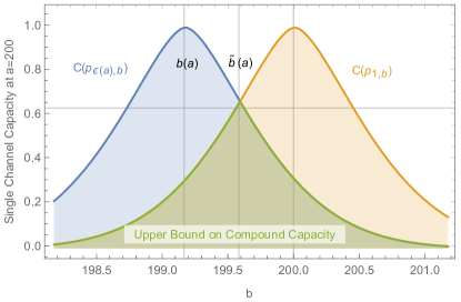
Figure 1: Figure 1: Numerical Estimates on Single Channel Capacities and on Compound Channel Capacity for $a=200$ and ${\varepsilon}={\varepsilon}(a)\approx 0.996$.

Let $\delta>0$, $a\in\mathbb{R}$ and ${\varepsilon}\in(0,1)$. Set $b=\sqrt{{\varepsilon}}a$. We explain below how this choice of $b$ is both almost-optimal for $\mathcal{N}_{\varepsilon}$ at high power levels $a$ and yet highly non-optimal for the compound channel $\mathcal{N}$. With our choice of $b$ it holds

$$p_{{\varepsilon},b}(0|0)=1,\qquad\qquad\qquad p_{{\varepsilon},b}(0|1)=e^{-4{\varepsilon}\cdot a^{2}}$$ (49)

$$p_{1,b}(0|0)=e^{-a^{2}(\sqrt{{\varepsilon}}-1)^{2}},\qquad p_{1,b}(0|1)=e^{-a^{2}(\sqrt{{\varepsilon}}+1)^{2}}.$$ (50)

Define, for every $p\in[0,1]$, $w_{p}\in C(\{0,1\},\{0,1\})$ by

$$w_{p}(y|0)=p\delta_{0}(y)+p^{\prime}\delta_{1}(y),\qquad w_{p}(y|1)=\delta_{1}(y).$$ (51)

Let $c>0$. Choosing ${\varepsilon}={\varepsilon}(a)=((a-c)/a)^{2}$ we get $\lim_{a\to\infty}{\varepsilon}(a)=1$ and for every $a>0$ we have $b=b(a)=\sqrt{{\varepsilon}(a)}a=a-c$. It then holds uniformly for all $c>0$ that

$$\lim_{a\to\infty}\|p_{{\varepsilon}(a),b(a)}-w_{1}\|_{F}=0.$$ (52)

In addition,

$$p_{1,b}(0|0) =e^{-c^{2}},\qquad p_{1,b}(0|1)=e^{-(2a-c)^{2}}.$$ (53)

With the special choice $c=\sqrt{\ln 2}$ we get

$$\lim_{a\to\infty}\|p_{1,b(a)}-w_{2^{-1}}\|_{F}=0.$$ (54)

The compound channel capacity $C$ [4] is continuous. Therefore,

$$C(\{p_{1,b(a)},p_{{\varepsilon}(a),b(a)}\})\leq C(\{w_{2^{-1}},w_{1}\})+\delta$$ (55)

for large enough $a$. The channel $w_{2^{-1}}$ has capacity $\log 5/4$, therefore $C(\{w_{2^{-1}},w_{1}\})\leq\log 5/4$. It follows that there exists an $a_{1}>0$ such that for all $a>a_{1}$

$$C(\{p_{1,b(a)},p_{{\varepsilon}(a),b(a)}\})\leq\log 5/4+\delta,$$ (56)

and $a_{2}>0$ such that for all $a>a_{2}$

$$C(\{p_{{\varepsilon}(a),b(a)}\})\geq C(\{w_{1}\})-\delta=1-\delta.$$ (57)

Thus we can state: For all $a$ satisfying $a>a_{1}+a_{2}$, if we choose $b(a)$ as the Kennedy receiver parameter then $b(a)$ is almost-optimal for $p_{{\varepsilon}(a),b(a)}$ but (choosing $\delta$ small enough) leads to a capacity $<1/3$ for transmission over $\{p_{1,b(a)},p_{{\varepsilon}(a),b(a)}\}$.

Let us consider another choice for $b$ instead: Set $\tilde{b}(a)=((a-c)+a)/2=a-c/2$ then we get

$$p_{{\varepsilon}(a),\tilde{b}(a)}(0|0)=e^{-\tfrac{c^{2}}{4}},\ \ p_{{\varepsilon}(a),\tilde{b}(a)}(0|1)=e^{-(2a-\tfrac{3c}{2})^{2}}$$ (58)

$$p_{1,\tilde{b}(a)}(0|0)=e^{-(\tilde{b}(a)-a)^{2}},\ \ p_{1,\tilde{b}(a)}(0|1)=e^{-(2a-\tfrac{c}{2})^{2}}.$$ (59)

Therefore

$$\lim_{a\to\infty}\|p_{{\varepsilon}(a),\tilde{b}(a)}-w_{e^{-c^{2}/4}}\|_{F}=0,$$ (60)

$$\lim_{a\to\infty}\|p_{1,\tilde{b}(a)}-w_{e^{-c^{2}/4}}\|_{F}=0.$$ (61)

Thus for every $\delta>0$ there is an $a_{3}>0$ such that for all $a>a_{3}$

$$C(\{p_{{\varepsilon}(a),b(a)}\}) \geq 1-\delta$$ (62)

$$C(\{p_{1,b(a)},p_{{\varepsilon}(a),b(a)}\}) \leq 3^{-1}+\delta$$ (63)

$$C(\{p_{1,\tilde{b}(a)},p_{{\varepsilon}(a),\tilde{b}(a)}\}) \geq C(w_{e^{-\ln(2)/4}})-\delta.$$ (64)

Since $C(w_{e^{-\ln(2)/4}})\geq 1-h(e^{-\ln(2)/4})/2\geq 1-0.75\cdot 0.5\geq 0.625$ we have shown the existence of compound channels $\{p_{1,b(a)},p_{{\varepsilon}(a),b(a)}\}$ with choices for $b(a)$ which are almost-optimal for $\{p_{{\varepsilon}(a),b(a)}\}$ but perform strictly below optimal for $\{p_{1,b(a)},p_{{\varepsilon}(a),b(a)}\}$.

VII Conclusion

We have derived capacity formulas for classical-quantum compound channels of practical interest. Furthermore, we demonstrated a nontrivial choice of the displacement parameter of the Kennedy receiver when applied to a compound channel, therewith proposing the compound channel model as a tool for receiver design in applications under timing constraints, where adaptive adjustment of the receiver is not desirable.

VII-A Acknowledgements

This work was financed by the DFG via grant NO 1129/2-1 (JN) and by the BMBF via grant 16KIS0948 (AC). This project has received funding from the European Union’s Horizon 2020 research and innovation programme under the Marie Sklodowska-Curie grant agreement No 845255 (MR).

References

- [1] K. M. R. Audenaert. A sharp continuity estimate for the von neumann entropy. Journal of Physics A: Mathematical and Theoretical, 40(28):8127–8136, jun 2007.
- [2] I. Bjelakovic and H. Boche. Classical capacities of compound and averaged quantum channels. IEEE Transactions on Information Theory, 55(7):3360–3374, 2009.
- [3] I. Bjelakovic, H. Boche, G. Janßen, and Nötzel J. Arbitrarily varying and compound classical-quantum channels and a note on quantum zero-error capacities. Aydinian H., Cicalese F., Deppe C. (eds) Information Theory, Combinatorics, and Search Theory. Lecture Notes in Computer Science, 7777, 2013.
- [4] A.J. Thomasian D. Blackwell, L. Breiman. The capacity of a class of channels. Ann. Math. Stat., 30(4):1229–1241, 1959.
- [5] N. Datta and T. C. Dorlas. The coding theorem for a class of quantum channels with long-term memory. Journal of Physics A: Mathematical and Theoretical, 40(28), 2007.
- [6] D. Dequal, L. Trigo Vidarte, V. Roman Rodriguez, G. Vallone, P. Villoresi, A. Leverrier, and E. Diamanti. Feasibility of satellite-to-ground continuous-variable quantum key distribution. npj Quantum Information, 7, 2021.
- [7] S. J. Dolinar. Communication Sciences and Egineering. Research Laboratory of Electronics (RLE) at the Massachusetts Institute of Technology (MIT), 111:115, 1973.
- [8] M. Fannes. A continuity property of the entropy density for spin lattice systems. Communications in Mathematical Physics, 31:291–294, 1973.
- [9] V. Giovannetti, S. Guha, S. Lloyd, L. Maccone, J. H. Shapiro, and H. P. Yuen. Classical Capacity of the Lossy Bosonic Channel: The Exact Solution. Phys. Rev. Lett., 92(2):4, jan 2004.
- [10] M. Hayashi. Universal coding for classical-quantum channel. Communications in Mathematical Physics, 289(25):5807, 2009.
- [11] A.S. Holevo. Coding theorems for quantum channels. Russian Math. Surveys, 53(6):1295–1331, 1998.
- [12] R. S. Kennedy. Near-Optimum Receiver for the Binary Coherent State Quantum Channel. MIT Res. Lab. Electron. Q. Prog. Rep., 108:219, 1973.
- [13] S. Masahide, E. Hiroyuki, F. Mikio, K. Mitsuo, I. Toshiyuki, S. Ryosuke, and T. Morio. Quantum photonic network and physical layer security. Phil. Trans. R. Soc. A, 375, 2017.
- [14] M. E. Shirokov. Uniform finite-dimensional approximation of basic capacities of energy-constrained channels. Quantum Information Processing, 17:322, 2018.
- [15] M.E. Shirokov. Adaptation of the alicki-fannes-winter method for the set of states with bounded energy and its use. Reports on Mathematical Physics, 81(1):81 – 104, 2018.
- [16] A. Waseda, M. Sasaki, M. Takeoka, M. Fujiwara, M. Toyoshima, and A. Assalini. Numerical evaluation of ppm for deep-space links. J. Opt. Commun. Netw., 3(6):514–521, Jun 2011.
- [17] C. Weedbrook, S. Pirandola, R. García-Patrón, N. J. Cerf, T. C. Ralph, J. H. Shapiro, and S. Lloyd. Gaussian quantum information. Rev. Mod. Phys., 84(2):621–669, may 2012.
- [18] A. Wehrl. General properties of entropy. Rev. Mod. Phys., 50:221–260, Apr 1978.
- [19] A. Winter. Coding theorem and strong converse for quantum channels. IEEE Trans. Inf. Theory, 45(7):2481–2485, 1999.
- [20] A. Winter. Tight uniform continuity bounds for quantum entropies: conditional entropy, relative entropy distance and energy constraints. Communications in Mathematical Physics, 347(1):291–313, 2016.