Meta-Cal: Well-controlled Post-hoc Calibration by Ranking

Abstract

In many applications, it is desirable that a classifier not only makes accurate predictions, but also outputs calibrated posterior probabilities. However, many existing classifiers, especially deep neural network classifiers, tend to be uncalibrated. Post-hoc calibration is a technique to recalibrate a model by learning a calibration map. Existing approaches mostly focus on constructing calibration maps with low calibration errors, however, this quality is inadequate for a calibrator being useful. In this paper, we introduce two constraints that are worth consideration in designing a calibration map for post-hoc calibration. Then we present Meta-Cal, which is built from a base calibrator and a ranking model. Under some mild assumptions, two high-probability bounds are given with respect to these constraints. Empirical results on CIFAR-10, CIFAR-100 and ImageNet and a range of popular network architectures show our proposed method significantly outperforms the current state of the art for post-hoc multi-class classification calibration.

1 Introduction

Recent advances in machine learning have resulted in very high accuracy in many classification tasks. In the context of computer vision, there has been a steady increase in top-1 accuracy on ImageNet (Russakovsky et al., 2015) since AlexNet (Krizhevsky et al., 2012). While highly accurate models are desirable in general, in some applications, we want that the output of a classifier is a calibrated posterior probability. This is especially important in cost-sensitive classification tasks, such as medical diagnosis (Ma et al., 2017) and autonomous driving (Chen et al., 2015).

The goal of classification calibration is to obtain a probabilistic model that has low calibration error. A formal definition of calibration error will be given in Section 3. To achieve this objective, one can design models with intrinsically low calibration errors. These models (Wilson et al., 2016; Pereyra et al., 2017; Lakshminarayanan et al., 2016; Malinin & Gales, 2018; Milios et al., 2018; Maddox et al., 2019) are usually developed with a Bayesian nature and tend to be expensive to train and make inferences. On the other end of the spectrum, a post-hoc calibration method transforms outputs of an existing classification model into well-calibrated predictions by learning a trainable post-processing step. A lot of effort (Zhang et al., 2020; Guo et al., 2017; Ding et al., 2020; Patel et al., 2020; Wenger et al., 2020; Kull et al., 2019) has been done along this line given the design difficulties and computational burdens of the former approach. In this work, we focus on post-hoc multi-class calibration.

Among the existing literature on post-hoc calibration, some methods (Zhang et al., 2020; Guo et al., 2017; Ding et al., 2020; Patel et al., 2020) seek calibration maps that preserve classification accuracy, while some other works (Wenger et al., 2020; Kull et al., 2019) focus more on calibration error without explicitly enforcing accuracy-preservation. Compared with the latter, there is no potential accuracy drop in the former, but its family of calibration maps is less flexible. We will formalize the limitation of such a family by giving a lower bound of its calibration error in Proposition 2. In this work, we try to get the best of both worlds by combining an existing calibration model with a bipartite ranking model, and we call our proposed post-hoc calibration method Meta-Cal.

Similar to previous works (Wenger et al., 2020; Kull et al., 2019), Meta-Cal does not enforce the overall accuracy being kept. As we will show later in Section 4, such a calibrator can be of little importance even if its calibration error is low. Additional constraints should be taken into consideration. In this work, we introduce two constraints: (i) miscoverage rate, (ii) coverage accuracy. In Section 4.1 and Section 4.2, we show Meta-Cal has full control over these two constraints. An intuitive interpretation of the above two constraints is by considering a quality assurance (QA) system. In such a system, two desired properties are: (i) for products accepted by the QA system, their quality requirements are satisfied with high confidence, (ii) the QA system does not perform unnecessary rejection. The first point corresponds to the coverage accuracy of a calibration map and the second one corresponds to the miscoverage rate. Their formal definitions are given in Section 4. Our proposed Meta-Cal is constructed from a base calibrator and a ranking model. If this base calibration model is accuracy-preserving, it is guaranteed that Meta-Cal has an improved calibration error bound over it.

The main contributions of this paper are:

• A novel post-hoc calibration approach (Meta-Cal) for multi-class classification is proposed. Meta-Cal augments a base calibration model and obtains better calibration performance.

• Two practical constraints are investigated alongside Meta-Cal. We show how these constraints are incorporated in constructing our proposed calibrator. Theoretical results on high-probability bounds w.r.t. these constraints are presented.

• We show the effectiveness of our proposed approach and validate our theoretical claims through a series of empirical experiments.

In the next section, we briefly review post-hoc calibration methods for classification and bipartite ranking models. Necessary background, notation and assumptions that will be used throughout this paper are given in Section 3. Section 4 describes our proposed approach. Two practical constraints of Meta-Cal are discussed in Section 4.1 and Section 4.2 respectively. Empirical results are presented in Section 5. Finally, we conclude in Section 6.

2 Related Work

Post-hoc Calibration of Classifiers: Platt scaling (Platt, 1999; Lin et al., 2007) is proposed to learn a calibration transformation to map the outputs of a binary SVM into posterior probabilities. Extensions of Platt scaling for multi-class calibration include temperature scaling (Guo et al., 2017), ensemble temperature scaling (Zhang et al., 2020) and local temperature scaling (Ding et al., 2020). Different from the parametric approach adopted by Platt scaling, histogram binning (Zadrozny & Elkan, 2001) is a non-parametric post-hoc calibration method in binary settings. Two popular refinements of histogram binning are isotonic regression (Zadrozny & Elkan, 2002) and Bayesian binning into quantiles (Naeini et al., 2015). Platt scaling assumes scores of each class are Gaussian distributed, however, this assumption is hardly satisfied for many probabilistic classifiers. Motivated by this assumption violation, Beta calibration (Kull et al., 2017) is proposed and it assumes Beta distribution of scores within each class. For multi-class classification, Dirichlet calibration (Kull et al., 2019) is proposed as an extension of Beta calibration. More recently, a Gaussian Process based calibration method is presented in Wenger et al. (2020).

Bipartite Ranking: The problem of bipartite ranking has been studied for a long time. In bipartite ranking, one wants to compare or rank two different objects and decide which one is better. Burges et al. (2005) uses a neural network to model a ranking function and trains this network by gradient decent methods. Clémençon et al. (2008) defines a statistical framework for such ranking problems and provides several consistency results. Narasimhan & Agarwal (2013) investigates the relationship between binary classification and bipartite ranking. Our work is closely related to Narasimhan & Agarwal (2013) and we rely on the theoretical results presented there to construct a binary class probability estimation (CPE) model from a ranking model.

Selective Classification: Selective classification is a technique that augments a classifier with a reject option. The essence of selective classification is the trade-off between coverage and accuracy. El-Yaniv & Wiener (2010) lays the foundation for selective classification by characterizing the theoretical and practical boundaries of risk-coverage trade-offs. Geifman & El-Yaniv (2017) applies selective classification to deep neural networks. While the starting point of our work is to make improvements in post-hoc classification calibration under several practical constraints, it turns out that techniques present in this work can also be used in selective classification. Geifman & El-Yaniv (2017) gives a one-sided and tight high-probability risk bound, while we present two high probability bounds for miscoverage rate and coverage accuracy. It should be noted that definitions of risk and coverage in our setting are different from these two metrics defined in the context of selective classification (El-Yaniv & Wiener, 2010; Geifman & El-Yaniv, 2017), thus these bounds are not directly comparable.

3 Problem Formulation

In this section, we summarize some necessary background, notation and assumptions that will be used throughout this paper. Let $\mathcal{X}$ be the input space and $\mathcal{Y}=[k]\coloneqq\{1,\cdots,k\}$ be the label space in multi-class classification. We denote the $(k-1)$-simplex by $\Delta^{k}\coloneqq\{(p_{1},\cdots,p_{k})\mid\sum_{i\in[k]}p_{i}=1,p_{i}\in[0,1]\}$. Suppose a probabilistic classifier $f:\mathcal{X}\to\Delta^{k}$ is given and this classifier is trained on an i.i.d. data set following a joint distribution $\mathbb{P}(X,Y)$ on $\mathcal{X}\times\mathcal{Y}$. Let the random variable $X$ take values in input space $\mathcal{X}$, $Z=(Z_{1},\cdots,Z_{k})$ be the output of $f$ applied to $X$, $\hat{Z}=\max_{i\in[k]}Z_{i}$ be the confidence score and $\hat{Y}=\operatorname*{arg\,max}_{i\in[k]}Z_{i}$ be the prediction of $X$. Whenever there is a tie, it is broken uniformly at random. To measure the level of calibration, following Naeini et al. (2015); Kumar et al. (2019); Wenger et al. (2020), the calibration error is defined in Definition 1.

Definition 1 (Calibration error).

The $L_{p}$ calibration error of $f$ with $p\geq 1$ is:

$$\operatorname{CE}_{p}(f)=\mathbb{E}\left[\left|\mathbb{E}\left(\mathds{1}(Y=\hat{Y})\mid\hat{Z}\right)-\hat{Z}\right|^{p}\right]^{1/p},$$ (1)

where the expectation is taken with respect to $\mathbb{P}(X,Y)$.

If the calibration error of a model $f$ is zero, we say $f$ is perfectly calibrated. In practice, $\operatorname{CE}_{p}(\cdot)$ is unobservable since it depends on the unknown joint distribution $\mathbb{P}(X,Y)$. To empirically estimate the calibration error based on a finite data set, prior works apply a fixed binning scheme $B\in\mathcal{B}$, where $\mathcal{B}$ is the family of binning schemes, on values of $\hat{Z}$ and calculate the difference between the accuracy and the average of confidence scores in every bin. An example family for a binning scheme is a partition of the interval $[0,1]$. When $p=1$, the calibration error is also known as expected calibration error (ECE) (Guo et al., 2017) and an empirical estimator based on $B$ is denoted by $\widehat{\operatorname{ECE}}_{B}$. Although it is known that $\widehat{\operatorname{ECE}}_{B}$ is a biased estimation (Kumar et al., 2019; Zhang et al., 2020) of $\operatorname{ECE}$ and its magnitude can be hard to interpret, in this work, we use this binned estimator to measure the level of calibration due to its simplicity and popularity.

In the post-hoc calibration problem, one wants to find a function that transforms the outputs of $f$ to make the final model better calibrated. Formally, a calibration map is a function $g:\Delta^{k}\to\Delta^{k}$. The goal is to learn a mapping $g\in\mathcal{G}$ on a finite calibration data set $\{(x_{i},y_{i})\}_{i=1}^{n}$ that is drawn i.i.d. from the joint distribution $\mathbb{P}(X,Y)$ so that the composition $g\circ f$ has a small calibration error, where $\mathcal{G}$ is the calibration family.

In the problem of bipartite ranking, we want to find a ranking model $h:\mathcal{X}\to\mathbb{R}$ that ranks positive examples and negative ones so that the positive examples have higher scores with a high probability. Formally, one wants to minimize the following ranking risk (Narasimhan & Agarwal, 2013; Clémençon et al., 2008):

$$L(f)=\mathbb{P}((\epsilon-\epsilon^{\prime})\cdot(h(X)-h(X^{\prime}))),$$

where $(X,\epsilon),(X^{\prime},\epsilon^{\prime})$ are i.i.d. pairs taking values in $\mathcal{X}\times\{-1,+1\}$. The ranking risk is the probability that $h$ ranks two randomly drawn pairs incorrectly (Clémençon et al., 2008). In this paper, if not stated otherwise, the random variable $\epsilon$ is a sign variable used to indicate whether $X$ is correctly classified or not by $f$, that is, $\epsilon=2\cdot\mathds{1}(Y\neq\hat{Y})-1$. In general, a bipartite ranking model is learnt using a consistent pairwise surrogate loss, such as exponential loss or logistic loss (Gao & Zhou, 2014).

In the following, we list some assumptions that will be used in Section 4.

Assumption 1.

Denote the marginal distribution of $X$ taking values in $\mathcal{X}$ by $\mathbb{P}(X)$. The induced distribution of $h(X)$ is continuous, where $h$ is a ranking model.

Assumption 2.

Let $h:\mathcal{X}\to[a,b]$ (where $a,b\in\mathbb{R}$, $a<b$) be any bounded-range ranking model. $\eta_{h}(s)=\mathbb{P}(\epsilon=1\mid h(x)=s)$ is square-integrable w.r.t. the induced density of $h(X)$.

The first assumption simply means for two independent samples from $\mathbb{P}(X)$, the probability of their ranking scores being equal vanishes. The second assumption is required by Narasimhan & Agarwal (2013) as we rely on their results.

4 Meta-Cal

In this section, we start by showing that the family of accuracy-preserving calibration maps has an inherent limitation (Proposition 2) and this motivates us to combine a bipartite ranking model with an existing calibration model. Then we demonstrate that models with low calibration errors alone do not necessarily indicate they are practical. Post-hoc calibration should be considered together with other factors. In this work, we investigate two useful constraints in Section 4.1 and Section 4.2, respectively: Miscoverage rate control and coverage accuracy control.

Proposition 2 (Lower bound of ECE).

Define $\mathcal{G}_{a}$ as the family of accuracy-preserving calibration maps, that is,

$$\mathcal{G}_{a}=\{g\in\mathcal{G}:\operatorname*{arg\,max}_{i\in[k]}f(X)_{i}=\operatorname*{arg\,max}_{i\in[k]}g(f(X))_{i}\}.$$

Then for all $g\in\mathcal{G}_{a}$

$$\sup_{B\in\mathcal{B}}\widehat{\operatorname{ECE}}_{B}(g\circ f)>\frac{1-\hat{\pi}_{0}}{k},$$ (2)

where $\widehat{\operatorname{ECE}}_{B}$ is estimated on a finite data set and $\hat{\pi}_{0}$ is the empirical accuracy of $f$ on the same data set. Further we can show $\forall B\in\mathcal{B},\forall g\in\mathcal{G}$,

$$\operatorname{ECE}(g\circ f)\geq\widehat{\operatorname{ECE}}_{B}(g\circ f).$$ (3)

All proofs are provided in LABEL:supp:proofs and we only describe a sketch of the proof here. The first step is to find the supremum of the binned estimator $\widehat{\operatorname{ECE}}_{B}(g\circ f)$ across all calibration maps $g\in\mathcal{G}_{a}$ and all binning schemes $B\in\mathcal{B}$. This is achieved using Minkowski’s inequality. The second step is showing this supremum is lower bounded by $(1-\hat{\pi}_{0})/k$. Unless $f$ is perfectly accurate, $(1-\hat{\pi}_{0})/k$ will be strictly positive. The last step is already given in Kumar et al. (2019) by applying Jensen’s inequality. We note bounding $\widehat{\operatorname{ECE}}_{B}(g\circ f)$ instead of its supremum makes little sense here since it is easy to construct a trivial $g\in\mathcal{G}_{a}$ and a binning scheme $B$ such that $\widehat{\operatorname{ECE}}_{B}(g\circ f)$ is exactly zero. In LABEL:supp:trivial-g, we give such a trivial construction. Proposition 2 makes it clear that an accuracy-preserving calibration has an inherent limitation. Such a calibration map cannot perfectly calibrate a classifier even if it is given the label information. To avoid potential confusion, we emphasize here the empirical estimator of ECE measures the top-label calibration error instead of the calibration error w.r.t. a fixed class.

In the following proposition, we show if a post-hoc calibration map is allowed to change the accuracy of the original classifier, it can achieve perfect calibration with the aid of a binary classifier.

Proposition 3 (Optimal calibration map).

Suppose realizations of $X\mid Y\neq\hat{Y}$ with positive labels and realizations of $X\mid Y=\hat{Y}$ with negative labels are separable and we are given a perfect binary classifier $\phi^{*}:\mathcal{X}\to\{-1,+1\}$ that is able to classify these two sets. For a new observation $x\sim X$, an optimal calibration map $g^{*}\in\mathcal{G}$ that minimizes $\sup_{B\in\mathcal{B},g\in\mathcal{G}}\widehat{\operatorname{ECE}}_{B}(g\circ f)$ can be constructed using the following rules:

• if $\phi^{*}(x)=-1$, we let $\max_{i\in[k]}g^{*}(x)_{i}=1$

• if $\phi^{*}(x)=+1$, we let $\max_{i\in[k]}g^{*}(x)_{i}=\frac{1}{k}$

Proof.

The optimality of $g^{*}$ follows directly from the proof steps of Proposition 2. ∎

We note $g^{*}\not\in\mathcal{G}_{a}$, since the used tie-breaking strategy is random at uniform, thus $g^{*}$ does not preserve the accuracy after the above calibration. It is straightforward to check the constructed $g^{*}$ in Proposition 3 has zero calibration error, that is $\operatorname{ECE}(g^{*}\circ f)=\sup_{B\in\mathcal{B}}\widehat{\operatorname{ECE}}_{B}(g^{*}\circ f)=0$.

However, it is unlikely that a perfect binary classifier can be obtained in practice and classification errors will occur when $\phi(X)\neq 2\cdot\mathds{1}(Y\neq\hat{Y})-1$. We denote the population Type I error (false positive error) and Type II error (false negative error) of $\phi$ by $R_{0}(\phi)$ and $R_{1}(\phi)$ respectively. In the following, we define the miscoverage rate and coverage accuracy of a calibration map $g$ constructed using the rules in Proposition 3. These two constraints will be used to construct the final calibration map.

Definition 4 (Miscoverage rate).

The miscoverage rate $F_{0}(g)$ of $g$ constructed using the rules in Proposition 3 is defined to be the Type I error of the binary classifier $\phi$ associated with $g$.

Definition 5 (Coverage accuracy).

The coverage accuracy $F_{1}(g)$ of $g$ constructed using the rules in Proposition 3 is defined to be the precision of the binary classifier $\phi$ associated with $g$.

The rational behind the above definitions will be illustrated by two examples later in this section. To be brief, these two constraints are necessary for a calibrator to be useful, if this calibrator cannot preserve the accuracy. The miscoverage rate of $g$ is the proportion of instances whose predictions are no longer correct after the calibration to instances whose predictions are originally correct before the calibration. The coverage accuracy of $g$ is the accuracy among covered instances (i.e. those instances classified as negative by the binary classifier) after the calibration. The correspondence between the Type I error (precision) of a binary classifier and the miscoverage rate (coverage accuracy) of a calibration map is due to the construction rules in Proposition 3.

Proposition 6.

Using the construction rules in Proposition 3, we can estimate the expected calibration error of $g$ on a finite data set:

$$\sup_{B\in\mathcal{B}}\widehat{\operatorname{ECE}}_{B}(g\circ f)=\hat{R}_{1}(\phi)\cdot(1-\hat{\pi}_{0}),$$

where $\hat{R}_{1}(\phi)$ is the empirical Type II error of $\phi$ which is trained following Proposition 3, $g$ is constructed using the rules in Proposition 3 and $\hat{\pi}_{0}$ is the empirical accuracy of $f$ on this finite data set.

The following two trivial calibration maps are used to illustrate the necessity of the above two constraints. These two calibrators have low calibration errors, but they are hardly useful.

High miscoverage rate: Based on the results in Proposition 6, to obtain a low calibration error, we could build a binary classifier with a low Type II error. This classifier has a potentially high Type I error, thus the miscoverage rate is potentially high as well. For example, we can select a small portion of negative instances and relabel the remaining instances as positive. Then a $1$-nearest neighbor classifier is such a classifier.

Low coverage accuracy: Regardless of the input, we let the output of a calibration map to be the marginal class distribution. The calibration error of this calibration map is equal to 0, but its coverage accuracy is low and equal to the proportion of the largest class.

Obviously, the above two constructions are of little consequence in practice. Another motivating example demonstrating the usefulness these two constraints is an automated decision model with human-in-the-loop (HIL). In such a model, on one hand, it is desirable that human interaction is as minimal as possible (low miscoverage rate). On the other hand, we hope this model can make accurate and reliable decisions (high coverage accuracy). We now describe how to construct a calibration map with a controlled miscoverage rate or a controlled coverage accuracy.

4.1 Miscoverage Rate Control

To control the miscoverage rate of our proposed calibration method, we need to construct a suitable binary classifier with a controlled Type I error. Such a classifier can be built using the following steps. Given a finite calibration data set $\{(x_{i},y_{i})\}_{i=1}^{n}$ that is drawn i.i.d. from the joint distribution $\mathbb{P}(X,Y)$ on $\mathcal{X}\times\mathcal{Y}$, we first create a binary classification data set $\{(x_{i},2\cdot\mathds{1}(y_{i}\neq\hat{y}_{i})-1)\}_{i=1}^{n}$, where $\hat{y}_{i}=\operatorname*{arg\,max}_{i\in[k]}f(x_{i})$ and $f$ is a multi-class classifier to be calibrated. Without loss of generality, we suppose the first $n_{1}$ inputs have negative labels and the last $n_{2}=n-n_{1}$ inputs have positive labels. Then we compute ranking scores on first $n_{1}$ inputs using a ranking model $h$ and denote these ranking scores as $\{r_{i}\}_{i=1}^{n_{1}}$, where $r_{i}=h(x_{i})$. Given a miscoverage rate tolerance $\alpha$, the desired binary classifier is constructed:

$$\hat{\phi}(x)=2\cdot\mathds{1}(h(x)>r_{(v)})-1,$$

where $v=\lceil(n_{1}+1)(1-\alpha)\rceil$, $r_{(v)}$ is the $v$-th order statistic of $\{r_{i}\}_{i=1}^{n_{1}}$, that is, $r_{(1)}\leq\cdots\leq r_{(n_{1})}$. We note under 1, the ranking model $h$ is continuous, thus $\mathbb{P}(r_{i}=r_{j})=0,\forall i,j\in[n_{1}]$ and the strict inequalities hold $r_{(1)}<\cdots<r_{(n_{1})}$. In the following Proposition 7, we show the miscoverage rate of our calibrator is well-controlled by proving that the Type I error of this constructed binary classifier is well-controlled.

Proposition 7 (Miscoverage rate control).

Under 1, given a finite test data set of size $m$ that is i.i.d. drawn from $\mathbb{P}(X,Y)$, the empirical miscoverage rate $\hat{F}_{0}(g)$ of $g$ on $D$ is well-controlled:

$$\mathbb{P}\left(\left|\hat{F}_{0}(g)-F_{0}(g)\right|\geq\delta\right) \approx\mathbb{P}\left(\left|R_{0}-F_{0}(g)\right|\geq\delta\right)$$ (4)

$$\leq 2\exp\left(-\frac{\delta^{2}}{2\sigma^{2}}\right),$$

where $F_{0}(g)$ is the population miscoverage rate of $g$, the random variable $R_{0}$ has a Normal distribution $\mathcal{N}(F_{0}(g),\sigma^{2})$, $\sigma^{2}=F_{0}(g)(1-F_{0}(g))/m_{1}$, $m_{1}\leq m$ is the number of samples whose predictions are correct.

Further, we have (Tong et al., 2018):

$$\mathbb{P}(F_{0}(g)>\alpha)=\sum_{j=v}^{n_{1}}\binom{n_{1}}{j}(1-\alpha)^{j}\alpha^{n_{1}-j},$$ (5)

where $v=\lceil(n_{1}+1)(1-\alpha)\rceil$.

Equation 5 is given in Tong et al. (2018) and we adapt it here for our purpose. Essentially it means the population miscoverage rate is smaller than the predefined miscoverage rate tolerance with a high probability. A rough estimation of the miscoverage rate of $g$ is $\lfloor(1+n)\alpha\rfloor/(1+n_{1})\leq\alpha$. Although the miscoverage rate of our constructed calibration map can be well-controlled using the above constructed binary classifier, there is no such a guarantee that the Type II error of $\hat{\phi}$ is also well-controlled. Combining the results shown in Proposition 6, it can be seen that the empirical ECE depends solely on $\hat{R}_{1}(\phi)$, since $\hat{\pi}_{0}$ is a constant given a finite data set. Thus we cannot make sure the empirical calibration error is small if we keep using the construction rules shown in Proposition 3.

A simple refinement to the above issue is to utilize a separate calibration model $g_{m}\in\mathcal{G}$ and the updated construction rules for a calibration map are listed in the following:

• if $\hat{\phi}(x)=-1$, we let $g(x)=g_{m}(x)$,
  

• if $\hat{\phi}(x)=+1$, we let $\max_{i\in[k]}g(x)_{i}=\frac{1}{k}$.

Now it is clear why we call our post-hoc calibration approach Meta-Cal, since our calibrator is built from a base calibration map. The rationality of the above updated rules is shown in Proposition 8.

Proposition 8 (Lower bound of Meta-Cal).

Suppose the base calibration map $g_{m}\in\mathcal{G}_{a}$ and $g$ is constructed using the above updated rules, then:

$$\sup_{B\in\mathcal{B}}\widehat{\operatorname{ECE}}_{B}(g\circ f)>w\frac{1-\hat{\pi}_{0}}{k},$$ (6)

where $w=(1-\hat{R}_{0}(\hat{\phi}))\hat{\pi}_{0}+\hat{R}_{1}(\hat{\phi})(1-\hat{\pi}_{0})<1$, $\hat{R}_{0}(\hat{\phi})$ and $\hat{R}_{1}(\hat{\phi})$ are empirical Type I error and Type II error of $\hat{\phi}$ respectively, $\hat{\pi}_{0}$ is the empirical accuracy of $f$ on a finite data set.

The result in Proposition 8 should be compared to the lower bound shown in Proposition 2. It can be seen that the calibration map constructed by Meta-Cal has an improved calibration error lower bound, compared with its accuracy-preserving base calibrator. Proposition 8 should also be compared with Proposition 6. From Equation 6, using the decomposition $\frac{w}{k}=\frac{(1-\hat{R}_{0}(\hat{\phi}))\hat{\pi}_{0}}{k}+\frac{\hat{R}_{1}(\hat{\phi})(1-\hat{\pi}_{0})}{k}$, we see the influence of the Type II error has been effectively diluted. This is desirable since we only have control over the Type II error of $\hat{\phi}$.

At the same time, the miscoverage rate of our constructed calibrator is well-controlled. In Section 5, we empirically show that Meta-Cal outperforms other competing methods in terms of the empirical estimation of ECE. Algorithm 1 sketches the construction of Meta-Cal under a miscoverage rate constraint. For details of this construction, please see the first paragraph of Section 4.1.

Algorithm 1 Meta-Cal (miscoverage control)

1:  Input: Training data set $\{(x_{i},y_{i})\}_{i=1}^{n}$, miscoverage rate tolerance $\alpha$, base calibration model $g_{m}$, ranking model $h$.

2:  Output: Binary classifier $\hat{\phi}$, Meta-Cal calibration model $g$.

3:  Partition the training data set randomly into two parts. The first part has only negative ($\hat{Y}=Y$) samples. The second part contains both negative and positive samples ($\hat{Y}\neq Y$).

4:  Compute ranking scores on the first part using the ranking model $h$. Compute threshold $r^{*}$ based on $\alpha$.

5:  Construct a binary classifier $\hat{\phi}$ based on $r^{*}$.

6:  Train a base calibration model $g_{m}$ using samples whose scores are smaller than $r^{*}$ among the second part.

7:  Construct the final calibration map $g$ using updated rules.

4.2 Coverage Accuracy Control

In some applications, we are more interested in controlling the coverage accuracy of a calibration map instead of its miscoverage rate. To construct a calibration map with a controlled coverage accuracy, similar to Section 4.1, we need to build a suitable binary classifier. It will be convenient to introduce the concept of a calibrated binary CPE model (Narasimhan & Agarwal, 2013).

Definition 9 (Calibrated binary CPE model (Narasimhan & Agarwal, 2013)).

A binary class probability estimation (CPE) model $\hat{\eta}:\mathcal{X}\to[0,1]$ is said to be calibrated w.r.t. a probability $\mathbb{P}(X,\epsilon)$ on $\mathcal{X}\times\{-1,+1\}$ if:

$$\mathbb{P}(\epsilon=1\mid\hat{\eta}(x)=u)=u,\forall u\in\text{range}(\eta)$$

where $\text{range}(\hat{\eta})$ denotes the range of $\hat{\eta}$.

We note a calibrated binary CPE model is different from a perfectly calibrated model (Definition 1) in the binary setting. Before we state our bound for the coverage accuracy, we present two existence propositions.

Proposition 10 (Existence of a monotonically increasing CPE transformation).

Under 1 and 2, let $h:\mathcal{X}\to[a,b]$ (where $a,b\in\mathbb{R}$, $a<b$) be any bounded-range ranking model. There exists a monotonically increasing function $t:\mathbb{R}\to[0,1]$ such that $t\circ h$ resulting from composing $t$ and $h$ is a calibrated binary CPE model.

Proof.

The existence of such a monotonically increasing CPE transformation directly follows by combining the results of Narasimhan & Agarwal (2013, Lemma 13) and Narasimhan & Agarwal (2013, Definition 12). ∎

Proposition 11 (Existence of a monotonically decreasing coverage accuracy transformation).

Under 1 and 2, let $h:\mathcal{X}\to[a,b]$ (where $a,b\in\mathbb{R}$, $a<b$) be any bounded-range ranking model. There exists a monotonically decreasing function $l:\mathbb{R}\to[0,1]$ such that $l(s)$ is the coverage accuracy of a calibration map $g$ which is constructed using the binary classifier $\hat{\phi}(x)=2\cdot\mathds{1}(h(x)>s)-1$.

Proof.

From Proposition 10, there exists a monotonically increasing $t$ such that $t\circ h$ is a calibrated binary CPE model. Let $\mathcal{E}_{h}(s)=\mathbb{P}(\epsilon=1\mid h(x)<s)$, since $t$ is monotonically increasing, we have:

$$\mathcal{E}_{h}(s)=\mathbb{P}(\epsilon=1\mid t(h(x))<t(s)).$$

Because $t\circ h$ is a calibrated binary CPE model, using Definition 9, we further have:

$$\mathcal{E}_{h}(s)=\int_{c}^{t(s)}udu=\frac{1}{2}t(s)^{2}-\text{constant}$$

where $c$ is a constant.

From Definition 5, the desired coverage accuracy transformation is:

$$l(s)=1-\mathcal{E}_{h}(s)=\text{constant}-\frac{1}{2}t(s)^{2}.$$

Since $t(s)\geq 0,\forall s\in\mathbb{R}$ and $t(\cdot)$ is a monotonically increasing function, it is obvious that $l$ is a monotonically decreasing function. From the definition of $\mathcal{E}_{h}(s)$, the binary classifier that is used to construct $g$ is exactly $\hat{\phi}(x)=2\cdot\mathds{1}(h(x)>s)-1$. ∎

Based on the above two existence propositions, we describe a bound for the empirical coverage accuracy in Proposition 12.

Table 1: ECE comparison. Uncal, TS, ETS, GPC, MetaMis, MetaAcc denote no-calibration, temperature scaling, ensemble temperature scaling, Gaussian Process calibration, Meta-Cal under miscoverage rate constraint and Meta-Cal under coverage accuracy constraint respectively. Reported values are the average of 40 independent runs. All standard errors are less than $5e-4$.

Dataset	Network	Acc	Uncal	TS	ETS	GPC	MetaMis	MetaAcc
	DenseNet40	0.9242	0.05105	0.00510	0.00567	0.00634	0.00434	0.00355
	ResNet110	0.9356	0.04475	0.00781	0.00809	0.00684	0.00391	0.00441
	ResNet110SD	0.9404	0.04022	0.00439	0.00509	0.00364	0.00350	0.00315
CIFAR10	WideResNet32	0.9393	0.04396	0.00706	0.00712	0.00684	0.00485	0.00532
	DenseNet40	0.7000	0.21107	0.01067	0.01104	0.01298	0.01093	0.00793
	ResNet110	0.7148	0.18182	0.02037	0.02130	0.01348	0.01815	0.01441
	ResNet110SD	0.7283	0.15496	0.01043	0.01057	0.01265	0.01109	0.00733
CIFAR100	WideResNet32	0.7382	0.18425	0.01332	0.01351	0.00993	0.01332	0.01189
	DenseNet161	0.7705	0.05531	0.02053	0.02064	NA	0.01388	0.01248
ImageNet	ResNet152	0.7620	0.06290	0.02023	0.02004	NA	0.01360	0.01138

Proposition 12 (Coverage accuracy control).

Under 1 and 2, the empirical coverage accuracy $\hat{F}_{1}(g)$ of $g$ on a finite test data set of size $m$ that is drawn i.i.d. from $\mathbb{P}(X,Y)$ is well-controlled:

$$\mathbb{P}\left(\left|\hat{F}_{1}(g)-\beta\right|\geq\delta\right) \approx\mathbb{P}\left(\left|R_{1}-\beta\right|\geq\delta\right)$$

$$\leq 2\exp\left(-\frac{m_{1}\delta^{2}}{2\beta(1-\beta)}\right),$$ (7)

where $\beta$ is the desired coverage accuracy, the random variable $R_{1}$ has a Normal distributon $\mathcal{N}\left(\beta,\frac{\beta(1-\beta)}{m_{1}}\right)$, and $m_{1}\leq m$ is the number of samples whose ranking scores are smaller than $l^{-1}(\beta)$ in the test data set.

Further, the desired binary classifier is:

$$\hat{\phi}(x)=2\cdot\mathds{1}(h(x)>l^{-1}(\beta))-1.$$ (8)

Algorithm 2 Meta-Cal (coverage accuracy control)

1:  Input: Training data set $\{(x_{i},y_{i})\}_{i=1}^{n}$, desired coverage accuracy $\beta$, base calibration model $g_{m}$, ranking model $h$.

2:  Output: Binary classifier $\hat{\phi}$, Meta-Cal calibration model $g$.

3:  Randomly split the training data set into two parts.

4:  Estimate the coverage accuracy transformation $\hat{l}$ on the first part.

5:  Compute a threshold $r^{*}=\hat{l}^{-1}(\beta)$ based on the estimated $\hat{l}$ and $\beta$.

6:  Construct a binary classifier $\hat{\phi}$ based on $r^{*}$.

7:  Train a base calibration model $g_{m}$ using samples among the second part whose scores are smaller than $r^{*}$.

8:  Construct the final calibration map $g$ using updated rules.

It should be noted that among all calibration maps whose coverage accuracy is higher than $\beta$, the calibration map constructed using the binary classifier in Equation 8 has the smallest miscoverage rate. In the following, we describe how to estimate the monotonically decreasing function $l$ in practice. Given a finite calibration data set $\{(x_{i},y_{i})\}_{i=1}^{n}$ that is drawn i.i.d. from the joint distribution $\mathbb{P}(X,Y)$ on $\mathcal{X}\times\mathcal{Y}$: Firstly the ranking scores $\{r_{i}\}_{i=1}^{n}$, where $r_{i}=h(x_{i})$, are computed using our ranking model $h$. Then a set of bins $\{I_{1},\cdots,I_{b}\}$ to partition $\{r_{i}\}_{i=1}^{n}$ is constructed through uniform mass binning (Zadrozny & Elkan, 2001). For a given $j\in\{1,\cdots,b\}$, let $l_{j}^{(s)}$ and $l_{j}^{(a)}$ denote the average of ranking scores on $I_{j}$ and $f$’s accuracy on $\{I_{1},\cdots,I_{j}\}$ respectively. Finally a decreasing isotonic regression model is fitted on $\{(l_{j}^{(s)},l_{j}^{(a)})\}_{j=1}^{b}$ and the fitted model is an estimation of $l$.  Algorithm 2 sketches the construction of Meta-Cal under the coverage accuracy constraint.

Several remarks are made to conclude this section. (i) The miscoverage rate bound holds for all base calibration maps. The coverage accuracy bound requires the base calibrator to preserve the accuracy. (ii) These two bounds do not depend on the metric used to evaluate the level of calibration, no matter whether it is top-label calibration error (which we use in this paper) or marginal calibration error (Kumar et al., 2019; Kull et al., 2019). (iii) To ensure the independence assumption, the training data of Meta-Cal should be different from the data set used to train the multi-class classifier.

5 Experiments

In this section, we present empirical results on a set of multi-class classifiers. Firstly, we compare our our proposed Meta-Cal described in Section 4 with several baselines. Then we validate the two constraints investigated in this work are well satisfied in Section 5.2.

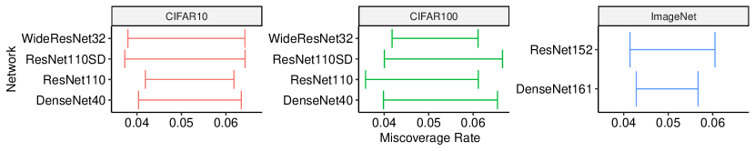
Figure 1: Empirical miscoverage rate. The error bars show $\pm 2$ standard deviation of 40 independent runs. The desired miscoverage rates for CIFAR-10, CIFAR-100 and ImageNet are all set to be $0.05$.

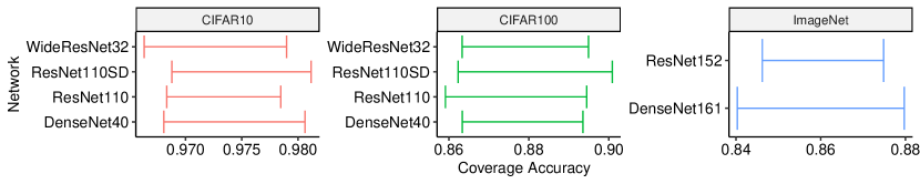
Figure 2: Empirical coverage accuracy. The error bars show $\pm 2$ standard deviation of 40 independent runs. The desired coverage accuracy for CIFAR-10, CIFAR-100 and ImageNet are set to be $0.97$, $0.87$ and $0.85$, respectively.

5.1 Calibrating Neural Networks

In this section, we compare our approach with other methods of post-hoc multi-class calibration. Following previous works (Guo et al., 2017; Kull et al., 2019; Zhang et al., 2020; Wenger et al., 2020), we report calibration results on several neural network classifiers trained on CIFAR-10, CIFAR-100 (Krizhevsky, 2009) and ImageNet (Deng et al., 2009). For CIFAR-10 and CIFAR-100, the following networks are used: DenseNet (Huang et al., 2016a), ResNet (He et al., 2015), ResNet with stochastic depth (Huang et al., 2016b), WideResNet (Zagoruyko & Komodakis, 2016). 45000 out of 60000 images are used for training these classifiers. The remaining 15000 images are held out for training and evaluating post-hoc calibration methods. The training details are given in LABEL:supp:train-detials. These 15000 samples are randomly split into 5000/10000 samples to train and evaluate a post-hoc calibration method. For ImageNet, we use pre-trained DenseNet-161 and ResNet-152 from PyTorch (Paszke et al., 2019). 50000 images in the validation set are used for training and evaluating post-hoc calibration methods. To train and test a calibration map, we randomly split these samples into 25000/25000 images.

The following post-hoc algorithms are used for comparison: temperature scaling (Guo et al., 2017), ensemble temperature scaling (Zhang et al., 2020), Gaussian Process calibration (Wenger et al., 2020). The Dirichlet calibration (Kull et al., 2019) is not included in our empirical comparison, since on the neural network classifiers we considered in this paper, its performance is consistently worse than other methods (Zhang et al., 2020).

To construct a calibration map using our proposed Meta-Cal, firstly we need to decide which base calibrator to use. Throughout the experimental part of this paper, we use temperature scaling since: (i) it is the most computationally efficient approach among the above baselines, and (ii) it can be seen from Proposition 8 that Meta-Cal augments the performance of temperature scaling, since it is an accuracy-preserving calibration map. Secondly a ranking model is required to construct a desired binary classifier based on different constraints. In this paper, we define the ranking model as the entropy of the output of an uncalibrated probabilistic classifier, that is, given $X\in\mathcal{X}$, we define $h(X)=-\sum_{i\in[k]}f(X)_{i}\log f(X)_{i}$. An alternative way is to learn a ranking model using a consistent ranking algorithm (Clémençon et al., 2008) on a separate data set. A potential advantage of this approach is the constructed binary classifier has a lower Type II error, thus from Proposition 6, the worst-case estimation of expected calibration error can be improved. A disadvantage of this approach is a separate data set is required to learn a ranking model and this effectively means we have less samples to train a calibration model.

The experimental configurations specific to our proposed approach are as follows. For Meta-Cal under the miscoverage rate constraint, we set the miscoverage rate tolerance to be $0.05$ for all neural network classifiers and all data sets used in the experiments. For Meta-Cal under the coverage accuracy constraint, we set the desired coverage accuracy to be $0.97$, $0.87$, $0.85$ for CIFAR-10, CIFAR-100 and ImageNet, respectively. For reference, the original accuracy for each configuration is shown in the third column in Table 1. In both settings, we randomly select $1/10$ samples (up to 500 samples) from the calibration data set to construct a binary classifier or estimate the coverage accuracy transformation function.

Table 2: Time comparison (s). Reported values are the average of 40 independent runs.

Dataset	Network	Uncal	TS	ETS	GPC	MetaMis	MetaAcc
	DenseNet40	0.004	0.074	0.143	4.722	0.102	0.094
	ResNet110	0.004	0.066	0.050	5.255	0.127	0.084
	ResNet110SD	0.004	0.075	0.148	5.401	0.101	0.090
CIFAR10	WideResNet32	0.004	0.078	0.133	5.116	0.105	0.093
	DenseNet40	0.014	0.492	0.492	40.218	0.470	0.336
	ResNet110	0.026	0.426	1.404	42.118	0.408	0.299
	ResNet110SD	0.015	0.357	0.931	40.867	0.421	0.327
CIFAR100	WideResNet32	0.014	0.431	0.708	44.882	0.467	0.353
	DenseNet161	0.304	12.707	99.488	NA	13.573	9.903
ImageNet	ResNet152	0.309	15.624	111.589	NA	12.581	8.426

The comparison results of different calibration methods are shown in Table 1. The empirical ECE are esitmated with 15 equal-width bins and ECE values reported in Table 1 are the average of 40 independent runs. Since GPC does not converge on ImageNet, its results on ImageNet are marked as NA in Table 1. We note CE loss instead of MSE in optimizing ETS.

From Table 1, it can be seen that our proposed method Meta-Cal performs much better w.r.t. the empirical ECE in almost all configurations. It should be noted that Table 1 should be interpreted in a careful way, since our proposed method works in a novel setting, that is, post-hoc calibration under constraints. Essentially, we can interpret the improved calibration is due to the miscoverage price we pay. It is worth noting that after calibration, GPC has an around $0.2\%$ accuracy drop in ResNet110 and ResNet110SD on CIFAR-10 data set. It is possible that GPC is trading off accuracy for calibration in an implicit and uncontrolled way.  Table 2 shows the running time of different calibration methods. It can be seen Meta-Cal has little overhead over its base calibrator (TS in our case). Sometimes Meta-Cal takes less than time than TS because its base calibrator is optimized on a subset of the whole calibration data set.

5.2 Verifying Constraints

In this section, we empirically verify whether constraints of miscoverage rate and coverage accuracy are satisfied. The purpose of this section is to support our theoretical claims in Section 4.1 and Section 4.2.

The error bar plot in Figure 1 depicts $\pm 2$ standard deviations of the empirical miscoverage rate over 40 independent runs. It can be seen from Figure 1 that the miscoverage rate is well-controlled given a miscoverage rate tolerance equal to $0.05$. In Figure 2, the $\pm 2$ standard deviation of the empirical coverage accuracy is illustrated. Given the desired coverage accuracies are set to be $0.97$, $0.87$ and $0.85$ for CIFAR-10, CIFAR-100 and ImageNet, respectively, it can be seen that the coverage accuracy is well-controlled.

6 Conclusion

In this work, we propose Meta-Cal: a post-hoc calibration method for multi-class classification under practical constraints, including miscoverage rate and coverage accuracy. Our proposed approach can augment an accuracy-preserving calibration map and improve its calibration performance. Contrary to post-hoc calibration methods that cannot preserve accuracy, our approach has full control over coverage accuracy. A series of theoretical results are given to show the validity of Meta-Cal. Empirical results on a range of neural network classifiers on several popular computer vision data sets show our approach is able to improve an existing calibration method.

Acknowledgements

Xingchen Ma is supported by Onfido. This research received funding from the Flemish Government under the “Onderzoeksprogramma Artificiële Intelligentie (AI) Vlaanderen” programme.

See pages - of icml2021-supp

References

- Burges et al. (2005) Burges, C., Shaked, T., Renshaw, E., Lazier, A., Deeds, M., Hamilton, N., and Hullender, G. Learning to rank using gradient descent. In Proceedings of the 22nd International Conference on Machine Learning, ICML ’05, pp. 89–96, New York, NY, USA, August 2005. Association for Computing Machinery. ISBN 978-1-59593-180-1. doi: 10.1145/1102351.1102363.
- Chen et al. (2015) Chen, C., Seff, A., Kornhauser, A., and Xiao, J. DeepDriving: Learning Affordance for Direct Perception in Autonomous Driving. In 2015 IEEE International Conference on Computer Vision (ICCV), pp. 2722–2730, December 2015. doi: 10.1109/ICCV.2015.312.
- Clémençon et al. (2008) Clémençon, S., Lugosi, G., and Vayatis, N. Ranking and Empirical Minimization of U-statistics. Annals of Statistics, 36(2):844–874, April 2008. ISSN 0090-5364, 2168-8966. doi: 10.1214/009052607000000910.
- Deng et al. (2009) Deng, J., Dong, W., Socher, R., Li, L.-J., Li, K., and Fei-Fei, L. Imagenet: A large-scale hierarchical image database. In 2009 IEEE conference on computer vision and pattern recognition, pp. 248–255. Ieee, 2009.
- Ding et al. (2020) Ding, Z., Han, X., Liu, P., and Niethammer, M. Local Temperature Scaling for Probability Calibration. arXiv:2008.05105 [cs], August 2020.
- El-Yaniv & Wiener (2010) El-Yaniv, R. and Wiener, Y. On the Foundations of Noise-free Selective Classification. Journal of Machine Learning Research, 11(53):1605–1641, 2010.
- Gao & Zhou (2014) Gao, W. and Zhou, Z.-H. On the Consistency of AUC Pairwise Optimization. arXiv:1208.0645 [cs, stat], July 2014.
- Geifman & El-Yaniv (2017) Geifman, Y. and El-Yaniv, R. Selective Classification for Deep Neural Networks. arXiv:1705.08500 [cs], June 2017.
- Guo et al. (2017) Guo, C., Pleiss, G., Sun, Y., and Weinberger, K. Q. On Calibration of Modern Neural Networks. In Proceedings of the 34th International Conference on Machine Learning - Volume 70, ICML’17, pp. 1321–1330. JMLR.org, 2017.
- He et al. (2015) He, K., Zhang, X., Ren, S., and Sun, J. Deep Residual Learning for Image Recognition. arXiv:1512.03385 [cs], December 2015.
- Huang et al. (2016a) Huang, G., Liu, Z., Weinberger, K. Q., and van der Maaten, L. Densely Connected Convolutional Networks. arXiv:1608.06993 [cs], August 2016a.
- Huang et al. (2016b) Huang, G., Sun, Y., Liu, Z., Sedra, D., and Weinberger, K. Q. Deep Networks with Stochastic Depth. In Leibe, B., Matas, J., Sebe, N., and Welling, M. (eds.), Computer Vision – ECCV 2016, Lecture Notes in Computer Science, pp. 646–661, Cham, 2016b. Springer International Publishing. ISBN 978-3-319-46493-0. doi: 10.1007/978-3-319-46493-0˙39.
- Krizhevsky (2009) Krizhevsky, A. Learning multiple layers of features from tiny images. Technical report, 2009.
- Krizhevsky et al. (2012) Krizhevsky, A., Sutskever, I., and Hinton, G. E. ImageNet Classification with Deep Convolutional Neural Networks. In Pereira, F., Burges, C. J. C., Bottou, L., and Weinberger, K. Q. (eds.), Advances in Neural Information Processing Systems 25, pp. 1097–1105. Curran Associates, Inc., 2012.
- Kull et al. (2017) Kull, M., Filho, T. S., and Flach, P. Beta calibration: A well-founded and easily implemented improvement on logistic calibration for binary classifiers. In Artificial Intelligence and Statistics, pp. 623–631. PMLR, April 2017.
- Kull et al. (2019) Kull, M., Perello Nieto, M., Kängsepp, M., Silva Filho, T., Song, H., and Flach, P. Beyond temperature scaling: Obtaining well-calibrated multi-class probabilities with Dirichlet calibration. In Wallach, H., Larochelle, H., Beygelzimer, A., d\textquotesingle Alché-Buc, F., Fox, E., and Garnett, R. (eds.), Advances in Neural Information Processing Systems 32, pp. 12316–12326. Curran Associates, Inc., 2019.
- Kumar et al. (2019) Kumar, A., Liang, P. S., and Ma, T. Verified Uncertainty Calibration. In Wallach, H., Larochelle, H., Beygelzimer, A., d\textquotesingle Alché-Buc, F., Fox, E., and Garnett, R. (eds.), Advances in Neural Information Processing Systems 32, pp. 3792–3803. Curran Associates, Inc., 2019.
- Lakshminarayanan et al. (2016) Lakshminarayanan, B., Pritzel, A., and Blundell, C. Simple and Scalable Predictive Uncertainty Estimation using Deep Ensembles. arXiv:1612.01474 [cs, stat], December 2016.
- Lin et al. (2007) Lin, H.-T., Lin, C.-J., and Weng, R. C. A note on Platt’s probabilistic outputs for support vector machines. Machine Learning, 68(3):267–276, October 2007. ISSN 1573-0565. doi: 10.1007/s10994-007-5018-6.
- Ma et al. (2017) Ma, X., Huang, D., Wang, Y., and Wang, Y. Cost-Sensitive Two-Stage Depression Prediction Using Dynamic Visual Clues. In Lai, S.-H., Lepetit, V., Nishino, K., and Sato, Y. (eds.), Computer Vision – ACCV 2016, Lecture Notes in Computer Science, pp. 338–351, Cham, 2017. Springer International Publishing. ISBN 978-3-319-54184-6. doi: 10.1007/978-3-319-54184-6˙21.
- Maddox et al. (2019) Maddox, W., Garipov, T., Izmailov, P., Vetrov, D., and Wilson, A. G. A Simple Baseline for Bayesian Uncertainty in Deep Learning. arXiv:1902.02476 [cs, stat], December 2019.
- Malinin & Gales (2018) Malinin, A. and Gales, M. Predictive Uncertainty Estimation via Prior Networks. In Bengio, S., Wallach, H., Larochelle, H., Grauman, K., Cesa-Bianchi, N., and Garnett, R. (eds.), Advances in Neural Information Processing Systems 31, pp. 7047–7058. Curran Associates, Inc., 2018.
- Milios et al. (2018) Milios, D., Camoriano, R., Michiardi, P., Rosasco, L., and Filippone, M. Dirichlet-based Gaussian Processes for Large-scale Calibrated Classification. In Bengio, S., Wallach, H., Larochelle, H., Grauman, K., Cesa-Bianchi, N., and Garnett, R. (eds.), Advances in Neural Information Processing Systems 31, pp. 6005–6015. Curran Associates, Inc., 2018.
- Naeini et al. (2015) Naeini, M. P., Cooper, G. F., and Hauskrecht, M. Obtaining well calibrated probabilities using bayesian binning. In Proceedings of the Twenty-Ninth AAAI Conference on Artificial Intelligence, AAAI’15, pp. 2901–2907, Austin, Texas, January 2015. AAAI Press. ISBN 978-0-262-51129-2.
- Narasimhan & Agarwal (2013) Narasimhan, H. and Agarwal, S. On the Relationship Between Binary Classification, Bipartite Ranking, and Binary Class Probability Estimation. Advances in Neural Information Processing Systems, 26:2913–2921, 2013.
- Paszke et al. (2019) Paszke, A., Gross, S., Massa, F., Lerer, A., Bradbury, J., Chanan, G., Killeen, T., Lin, Z., Gimelshein, N., Antiga, L., Desmaison, A., Kopf, A., Yang, E., DeVito, Z., Raison, M., Tejani, A., Chilamkurthy, S., Steiner, B., Fang, L., Bai, J., and Chintala, S. Pytorch: An imperative style, high-performance deep learning library. In Advances in Neural Information Processing Systems 32, pp. 8024–8035. Curran Associates, Inc., 2019.
- Patel et al. (2020) Patel, K., Beluch, W., Yang, B., Pfeiffer, M., and Zhang, D. Multi-Class Uncertainty Calibration via Mutual Information Maximization-based Binning. arXiv:2006.13092 [cs, stat], September 2020.
- Pereyra et al. (2017) Pereyra, G., Tucker, G., Chorowski, J., Kaiser, Ł., and Hinton, G. Regularizing Neural Networks by Penalizing Confident Output Distributions. arXiv:1701.06548 [cs], January 2017.
- Platt (1999) Platt, J. C. Probabilistic Outputs for Support Vector Machines and Comparisons to Regularized Likelihood Methods. In Advances in Large Margin Classifiers, pp. 61–74. MIT Press, 1999.
- Russakovsky et al. (2015) Russakovsky, O., Deng, J., Su, H., Krause, J., Satheesh, S., Ma, S., Huang, Z., Karpathy, A., Khosla, A., Bernstein, M., Berg, A. C., and Fei-Fei, L. ImageNet Large Scale Visual Recognition Challenge. International Journal of Computer Vision, 115(3):211–252, December 2015. ISSN 1573-1405. doi: 10.1007/s11263-015-0816-y.
- Tong et al. (2018) Tong, X., Feng, Y., and Li, J. J. Neyman-Pearson classification algorithms and NP receiver operating characteristics. Science Advances, 4(2), February 2018. ISSN 2375-2548. doi: 10.1126/sciadv.aao1659.
- Wenger et al. (2020) Wenger, J., Kjellström, H., and Triebel, R. Non-Parametric Calibration for Classification. In International Conference on Artificial Intelligence and Statistics, pp. 178–190, June 2020.
- Wilson et al. (2016) Wilson, A. G., Hu, Z., Salakhutdinov, R., and Xing, E. P. Stochastic Variational Deep Kernel Learning. arXiv:1611.00336 [cs, stat], November 2016.
- Zadrozny & Elkan (2001) Zadrozny, B. and Elkan, C. Obtaining calibrated probability estimates from decision trees and naive Bayesian classifiers. In Proceedings of the Eighteenth International Conference on Machine Learning, ICML ’01, pp. 609–616, San Francisco, CA, USA, June 2001. Morgan Kaufmann Publishers Inc. ISBN 978-1-55860-778-1.
- Zadrozny & Elkan (2002) Zadrozny, B. and Elkan, C. Transforming classifier scores into accurate multiclass probability estimates. In Proceedings of the Eighth ACM SIGKDD International Conference on Knowledge Discovery and Data Mining, KDD ’02, pp. 694–699, New York, NY, USA, July 2002. Association for Computing Machinery. ISBN 978-1-58113-567-1. doi: 10.1145/775047.775151.
- Zagoruyko & Komodakis (2016) Zagoruyko, S. and Komodakis, N. Wide Residual Networks. arXiv:1605.07146 [cs], May 2016.
- Zhang et al. (2020) Zhang, J., Kailkhura, B., and Han, T. Y.-J. Mix-n-Match: Ensemble and Compositional Methods for Uncertainty Calibration in Deep Learning. arXiv:2003.07329 [cs, stat], June 2020.