Localization of Invariable Sparse Errors in Dynamic Systems

Localization of Invariable Sparse Errors in Dynamic Systems
Accepted version of DOI:10.1109/TCNS.2021.3077987m;
Copyright: 978-1-7281-3949-4/19/$31.00 ©2021 IEEE

Abstract

Understanding the dynamics of complex systems is a central task in many different areas ranging from biology via epidemics to economics and engineering. Unexpected behaviour of dynamic systems or even system failure is sometimes difficult to comprehend. Such a data-mismatch can be caused by endogenous model errors including misspecified interactions and inaccurate parameter values. These are often difficult to distinguish from unmodelled process influencing the real system like unknown inputs or faults. Localizing the root cause of these errors or faults and reconstructing their dynamics is only possible if the measured outputs of the system are sufficiently informative.

Here, we present criteria for the measurements required to localize the position of error sources in large dynamic networks. We assume that faults or errors occur at a limited number of positions in the network. This invariable sparsity differs from previous sparsity definitions for inputs to dynamic systems. We provide an exact criterion for the recovery of invariable sparse inputs to nonlinear systems and formulate an optimization criterion for invariable sparse input reconstruction. For linear systems we can provide exact error bounds for this reconstruction method.

1 Introduction

In this paper, we study the localization and reconstruction of invariable sparse faults and model errors in complex dynamic networks described by ordinary differential equations (ODEs). Invariable sparsity means here that there is a maximum number of state variables (state nodes) $k$ affected by an error and that the set of these states targeted by errors is invariant in time. Typically, $k$ is much smaller than the total number of state nodes $N$. In contrast to fault isolation approaches [1, 2], we do not require the a priori specification of certain types of faults, but we allow for the possibility that each state node in the network can potentially be targeted by errors (or faults). The invariable sparse error assumption is often realistic in both the cases of a poor model and the fault detection context. Faults often affect only a small number of nodes in the network because the simultaneous failure of several components in a system is unlikely to occur spontaneously. For example, a hardware error or a network failure usually occurs at one or two points in the system, unless the system has been deliberately attacked simultaneously at several different positions. Similarly, gene mutations often affect a restricted number of proteins in a larger signal transduction or gene regulatory network. In the context of model error localization and reconstruction, the invariable sparsity assumption implies that the model is incorrect only at a limited number of positions or, alternatively, that small inaccuracies are ignored and that we focus only on the few (less than $k$) state variables with grossly misspecified governing equations.

A model error is often understood as a poor specification of the model structure, the interaction terms and the parameter values. These endogenous errors are then distinguished from exogenous influences acting on the real system including unknown inputs and faults. One could, however, regard unknown inputs and faults as part of the real system. Then, the absence of terms in the model representing inputs and faults can be considered as unmodelled dynamics or model error. This is in accordance with the fact that faults, model errors, and interactions with the environment can all mathematically be represented as unknown inputs to the system [3, 4, 5, 6, 7]. Thus, throughout this paper we use model error, fault, and unknown input as synonyms.

Sparsity of control inputs has been studied in previous publications in various contexts, which we can only briefly review here: Hands-off control is a paradigm to deal with limitations in equipment by searching for controls with minimum support per unit time [8, 9, 10]. For discrete time systems, sparsity is often defined by a maximum number inputs at each time instance [11, 12, 13]. Here, we consider the reconstruction of invariable sparse inputs in continuous time, which means that zero inputs remain zero throughout time. This is related to the problem of minimal controllability [14], where the aim is to find a minimum set of state variables to be targeted by a control, which renders the resulting system controllable [15].

To summarize, our main contributions are:

1. We provide a graphical criterion for the recovery of invariable sparse model errors, unknown inputs or faults in nonlinear dynamic systems. To derive this criterion, we combine structural control theory and gammoid theory to define sets of input states which are independent in the sense that they can independently be reconstructed. This abstraction allows us to transfer the concept of the spark from compressed sensing theory [16, 17, 18, 19] to nonlinear dynamic systems.

2. Computation of the spark can be very demanding in large systems. Therefore, we provide efficient approximations for the spark based on the concept of coherent input states for linear systems.

3. We provide a method for the recovery of invariable sparse inputs based on the solution of a convex optimisation problem. We propose a function space norm for model errors which promotes invariable sparsity. The resulting optimisation problem is different from the $L_{1}$ or $L_{1}/L_{2}$ regularization used in other sparse optimal control settings [8, 9, 10].

4. For linear systems, we also present a variant of the Restricted-Isometry-Property [20], which guarantees the recovery of invariable sparse inputs in the presence of measurement noise using our convex optimization method.

Please note that the proofs of all theorems can be found in the Supplemental Text.

2 Background

2.1 Open dynamic systems with errors and faults

The models we want to consider are dynamic input-output systems of the form

$$\dot{{\mbox{$x$}}}(t) ={\mbox{$f$}}({\mbox{$x$}}(t))+{\mbox{$w$}}(t)$$ (1)

$${\mbox{$x$}}(0) ={\mbox{$x$}}_{0}$$

$${\mbox{$y$}}(t) ={\mbox{$c$}}({\mbox{$x$}}(t)),$$

where ${\mbox{$x$}}(t)\subseteq\mathbb{R}^{N}$ denotes the state of the system at time $t\in[0,T]$ and ${\mbox{$x$}}_{0}\in\mathbb{R}^{N}$ is the initial state. The vector field $f$ encodes the model of the system and is assumed to be Lipshitz. The function ${\mbox{$c$}}:\mathbb{R}^{N}\to\mathbb{R}^{P}$ describes the measurement process and maps the system state $x$ to the directly observable output $y$.

Model errors are represented as unknown input functions ${\mbox{$w$}}:[0,T]\to\mathbb{R}^{N}$. This ansatz incorporates all types of errors, including missing and wrongly specified interactions, parameter errors [3, 21, 22, 5, 6, 23] as well as faults [1, 2] and unobserved inputs from the environment [7].

The system (1) can be seen as an input-output map $\Phi:\mathcal{W}\to\mathcal{Y},{\mbox{$w$}}\mapsto{\mbox{$y$}}$. The input space $\mathcal{W}=\mathcal{W}_{1}\oplus\ldots\oplus\mathcal{W}_{N}$ is assumed to be the direct sum of suitable (see below) function spaces $\mathcal{W}_{i},\,i=1,\ldots,N$. For zero errors ${\mbox{$w$}}\equiv{\mbox{$0$}}$ (i.e. ${\mbox{$w$}}(t)={\mbox{$0$}}\,\forall t\in[0,T]$) we call the system (1) a closed dynamic system. Please note that we do not exclude the possibility of known inputs for control, but we suppress them from our notation.

The residual between the measured output data ${\mbox{$y$}}^{\text{data}}(t)$ and the output ${\mbox{$y$}}^{(0)}(t)=\Phi({\mbox{$0$}})(t)$ of the closed system

$${\mbox{$r$}}(t):={\mbox{$y$}}^{\text{data}}(t)-{\mbox{$y$}}^{(0)}(t)$$ (2)

carries all the available information about the model error. To infer the model error aka unknown input ${\mbox{$w$}}(t)$ we have to solve the equation

$$\Phi({\mbox{$w$}})={\mbox{$y$}}^{\text{data}}$$ (3)

for $w$.

In general, there can be several solutions to the problem (3), unless we either measure the full state of the system or we restrict the set of unknown inputs $w$. In fault detection applications [1, 2], the restriction is given by prior assumptions about the states which are targeted by errors. We will use the invariable sparsity assumption instead. For both cases, we need some notation: Let $\mathcal{N}=\{1,2,\ldots,N\}$ be the index set of the $N$ state variables and $S\subseteq\mathcal{N}$ be a subset with complement $S^{c}=\mathcal{N}\setminus S$. By ${\mbox{$w$}}_{S}(t)$ we indicate the vector function obtained from ${\mbox{$w$}}(t)$ by setting the entries $({\mbox{$w$}}_{S})_{i}$ with $i\in S^{c}$ to the zero function. If $S$ is of minimal cardinality and ${\mbox{$w$}}_{S}={\mbox{$w$}}$ we call $S$ the support of $w$. The corresponding restriction on the input space is defined via

$$\mathcal{W}_{S}:=\left\{{\mbox{$w$}}\in\mathcal{W}\left|\,\text{supp}\,{\mbox{$w$}}\subseteq S\right.\right\}\,.$$ (4)

Thus, $S$ characterizes the states $x_{i}$ with $i\in S$ which can potentially be affected by a non-zero unknown input $w_{i}$. We will also refer to $S$ as the set of input or source nodes. The restricted input-output map $\Phi_{S}:\mathcal{W}_{S}\to\mathcal{Y}$ is again given by (1), but all input components ${\mbox{$w$}}_{i}$ with $i\not\in S$ are restricted to be zero functions.

Now, we can formally define invertibility [24, 25]:

Definition 1

The system (1) with input set $S$ and input-output map $\Phi$ is called invertible, if for two different solutions ${\mbox{$w$}}^{(1)},{\mbox{$w$}}^{(2)}\in\mathcal{W}_{S}$ of (3) and for any data set ${\mbox{$y$}}^{\text{data}}:[0,T]\to\mathbb{R}^{P}$ we have

$${\mbox{$w$}}^{(1)}(t)-{\mbox{$w$}}^{(2)}(t)={\mbox{$0$}}$$ (5)

almost everywhere in $[0,T]$.

In other words, invertibility guarantees that (3) with an input set $S$ has only one solution ${\mbox{$w$}}^{*}$ (up to differences of measure zero), which corresponds to the true model error. In the following, we mark this true model error with an asterisk, while $w$ without asterisk denotes an indeterminate input function.

2.2 Structural invertibility and independence of input nodes

There are several algebraic or geometric conditions for invertibility [24, 25, 26, 27, 28], which are, however, difficult to test for large systems and require exact knowledge of the systems equations (1), including all the parameters. Structural invertibility of a system is prerequisite for its invertibility and can be decided from a graphical criterion [29], see also Theorem 1 below. Before, we define the influence graph (see e.g. [15])

Definition 2

The influence graph $g=(\mathcal{N},\mathcal{E})$ of the system (1) is a digraph, where the set of nodes $\mathcal{N}=\{1,2,\ldots,N\}$ represents the $N$ state variables, ${\mbox{$x$}}=(x_{1},\ldots,x_{N})$, and the set of directed edges $\mathcal{E}=\{i_{1}\to l_{1},i_{2}\to l_{2},\ldots\}$ represents the interactions between those states in the following way: There is a directed edge $i\to l$ for each pair of state nodes $i,l\in\mathcal{N}$ if and only if $\frac{\partial f_{l}}{\partial x_{i}}({\mbox{$x$}})\neq 0$ for some $x$ in the state space $\mathcal{X}$.

In addition to the set of input nodes $S\subseteq\mathcal{N}$ we define the output nodes $Z\subseteq\mathcal{N}$ of the system (1). The latter are determined by the measurement function $c$. Without restriction of generality we assume in the following that a subset $Z\subseteq\{1,2,\ldots,N\}$ of $P$ state nodes are sensor nodes, i.e., they can directly be measured, which corresponds to $c_{i}({\mbox{$x$}})=x_{i}$ for $i\in Z$. All states $x_{l}$ with $l\not\in Z$ are not directly monitored.

A necessary criterion for structural invertibility is given by the following graphical condition [29]:

Theorem 1

Let $g=(\mathcal{N},\mathcal{E})$ be an influence graph and $S,Z\subseteq\mathcal{N}$ be known input and output node sets with cardinality $M=\text{card}\,S$ and $P=\text{card}\,Z$, respectively. If there is a family of directed paths $\Pi=\{\pi_{1},\ldots,\pi_{M}\}$ with the properties

1. each path $\pi_{i}$ starts in $S$ and terminates in $Z$,

2. any two paths $\pi_{i}$ and $\pi_{j}$ with $i\neq j$ are node-disjoint,

then the system is structurally invertible. If such a family of paths exists, we say $S$ is linked in $g$ into $Z$.

In the Supplemental Text we discuss why we have the strong indication that this theorem provides also a sufficient criterion for structural invertibility up to some pathological cases.

A simple consequence of this theorem is that for an invertible system, the number $P$ of sensor nodes cannot be smaller than the number of input nodes $M$. This is the reason, why for fault detection the set of potentially identifiable error sources $S$ is selected in advance [2]. Without a priori restriction on the set of potential error sources, we would need to measure all states. Please note that there are efficient algorithms to check, whether a system with a given influence graph $g$ and given input and sensor node set $S$ and $Z$ is invertible (see [7] for a concrete algorithm and references therein).

2.3 Independence of input nodes

If the path condition for invertibility in Theorem 1 is fulfilled for a given triplet $(S,g,Z)$ we can decide, whether the unknown inputs targeting $S$ can be identified in the given graph $g$ using the set of sensor nodes $Z$. Without a priori knowledge about the model errors, however, the input set $S$ is unknown as well. Therefore, we will consider the case that the input set $S$ is unknown in the results section. To this end, we define an independence structure on the union of all possible input sets:

Definition 3

The triple $\Gamma:=(\mathcal{L},g,Z)$ consisting of an influence graph $g=(\mathcal{N},\mathcal{E})$, an input ground set $\mathcal{L}\subseteq\mathcal{N}$, and an output set $Z$ is called a gammoid. A subset $S\subseteq\mathcal{L}$ is understood as an input set. An input set $S$ is called independent in $\Gamma$, if $S$ is linked in $g$ into $Z$.

The notion of (linear) independence of vectors is well known from vector space theory. For finite dimensional vector spaces, there is the rank-nullity theorem relating the dimension of the vector space to the dimension of the null space of a linear map. The difference between the dimension of the vector space and the null space is called the rank of the map. The main advantage of the gammoid interpretation lies in the following rank-nullity concept:

Definition 4

Let $\Gamma=(\mathcal{L},g,Z)$ be a gammoid.

1. The rank of a set $S\subseteq\mathcal{L}$ is the size of the largest independent subset $\tilde{S}\subseteq S$.

2. The nullity is defined by the rank-nullity theorem

   $$\text{rank}\,S+\text{null}\,S=\text{card}\,S\,.$$ (6)

Note that the equivalence of a consistent independence structure and a rank function (see definition 4 1.) as well as the existence of a rank-nullity theorem (see definition 4 2.) goes back to the early works on matroid theory [30]. It has already been shown [31] that the graph theoretical idea of linked sets (see definition 3) fulfils the axioms of matroid theory and therefore inherits its properties. The term gammoid for such a structure of linked sets was probably first used in [32] and since then investigated under this name, with slightly varying definitions. We find the formulation above to be suitable for our purposes (see also the Supplemental Text for more information about gammoids).

3 Results

Here, we consider the localization problem, where the input set $S$ is unknown. However, we make an invariable sparsity assumption by assuming that $S$ is a small subset of the ground set $\mathcal{L}\subseteq\mathcal{N}$.

Definition 5

The input signal $w$ with the input set $S$ is invariable $k$-sparse if the cardinality of $S$ is at most $k$.

Please note that invariable sparsity refers to the input set $S$, i.e., to the invariable support of the input $w$. This should not be confused with other sparsity definitions used for continuous time signals [8, 9, 10] which take the temporal support. Invariable sparse input functions ${\mbox{$w$}}(t)$ have zero components $w_{i}(t)=0$ for all times $t\in[0,T]$, if $i\in S^{c}$. Depending on the prior information, the ground set $\mathcal{L}$ can be the set of all state variables $\mathcal{N}$ or a subset.

The invariable sparsity assumption together with the definition of independence of input nodes in Definitions 3 and 4 can be exploited to generalize the idea of sparse sensing [16, 20, 17, 18] to the solution of the dynamic problem (3). Sparse sensing for matrices is a well established field in signal and image processing (see e.g. [18, 19]). There are, however, some nontrivial differences: First, the input-output map $\Phi$ is not necessarily linear. Second, even if $\Phi$ is linear, it is a compact operator between infinite dimensional vector spaces and therefore the inverse $\Phi^{-1}$ is not continuous. This makes the inference of unknown inputs $w$ an ill-posed problem, even if (3) has a unique solution [33].

3.1 Invariable sparse error localization and spark for nonlinear systems

Definition 3 enables us to transfer the concept of the spark [16] to dynamic systems:

Definition 6

Let $\Gamma=(\mathcal{L},g,Z)$ be a gammoid. The spark of $\Gamma$ is defined as the largest integer, such that for each input set $S\subseteq\mathcal{L}$

$$\text{card}\,S<\text{spark}\,\Gamma\,\Rightarrow\,\text{null}\,S=0\,.$$ (7)

Let’s assume we have a given dynamic system with influence graph $g=(\mathcal{N},\mathcal{E})$ and with an output set $Z\subset\mathcal{N}$. In addition, we haven chosen an input ground set $\mathcal{L}$. Together, we have the gammoid $\Gamma=(\mathcal{L},g,Z)$. The spark gives the smallest number of inputs that are dependent. As for the compressed sensing problem for matrices [16], we can use the spark to check, under which condition an invariable sparse solution is unique:

Theorem 2

For an input $w$ we denote $\|{\mbox{$w$}}\|_{0}$ the number of non-zero components. Assume $w$ solves (3). If

$$\|{\mbox{$w$}}\|_{0}<\frac{\text{spark}\,\Gamma}{2}\,,$$ (8)

then $w$ is the unique invariable sparsest solution.

This theorem provides a necessary condition for the localizability of an invariable $k$-sparse error in a nonlinear dynamic system. The analogous condition for sparse sensing of matrices is also sufficient [34, 35]. More research is needed to check whether this carries over to Theorem 2 for the dynamic systems setting.

For instance, if we expect an error or input to target a single state node like in Fig. 2(a), we have $\|{\mbox{$w$}}^{*}\|_{0}=1$ and we need $\text{spark}\,\Gamma\geq 3$ to pinpoint the exact position of the error in the network. If an edge in the network is the error source, then two nodes are affected and $\|{\mbox{$w$}}^{*}\|_{0}=2$. Such an error could be a misspecified reaction rate in a biochemical reaction or a cable break in an electrical network. To localize such an error we need $\text{spark}\,\Gamma\geq 5$.

For smaller networks like the one in Fig. 2(a), it is possible to exactly compute the spark (Definition 6) of a gammoid (Definition 3) using an combinatorial algorithm iterating over all possible input node sets. However, the computing time grows rapidly with the size of the network. Below we present bounds for the spark, which can efficiently be computed.

3.2 Coherence of potential input nodes in linear systems

So far we have given theorems for the localizability of invariable sparse errors in terms of the spark. However, computing the spark is again a problem whose computation time grows rapidly with increasing systems size. Now, we present a coherence measure between a pair of state nodes $i,j$ in linear systems indicating how difficult it is to decide whether a detected error is localized at $i$ or at $j$. The coherence provides a lower bound for the spark and can be approximated by an efficient shortest path algorithm. Computing the coherence for each pair of state nodes in the network yields the coherence matrix, which can be used to isolate a subset of states where the root cause of the error must be located.

If the system (1) is linear, i.e., ${\mbox{$f$}}({\mbox{$x$}})=A{\mbox{$x$}}$ and ${\mbox{$c$}}({\mbox{$x$}})=C{\mbox{$x$}}$, we can use the Laplace-transform

$$T(s)\tilde{{\mbox{$w$}}}(s)=\tilde{{\mbox{$y$}}}(s),\qquad s\in\mathbb{C}$$ (9)

to represent the input-output map $\Phi_{\mathcal{L}}$ by the $L\times P$-transfer matrix $T(s)$. The tilde denotes Laplace-transform. Again, we assume that $w_{i}\equiv 0$ for all $i\neq\mathcal{L}$ and $\tilde{{\mbox{$w$}}}(s)$ is the vector of Laplace-transforms of the components of $w$ which are in the ground set $\mathcal{L}$ . Recall that $L\leq N$ is the number of states in the ground set $\mathcal{L}$ and $P$ the number of measured outputs. As before, $\mathcal{L}=\mathcal{N}$ is still a possible special case.

We introduce the input gramian

$$G(s):=T^{*}(s)T(s)$$ (10)

where the asterisk denotes the hermitian conjugate. Note that the input gramian is an $L\times L$ matrix. Assume that we have chosen an arbitrary but fixed numbering of the states in the ground set, i.e., $\mathcal{L}=\{l_{1},\ldots,l_{L}\}$ is ordered.

Definition 7

Let $G$ be the input gramian of a linear dynamic system. We call

$$\mu_{ij}(s):=\frac{|G_{ij}(s)|}{\sqrt{G_{ii}(s)G_{jj}(s)}},\qquad s\in\mathbb{C}$$ (11)

the coherence function of nodes $l_{i}$ and $l_{j}$. We call

$$\mu(s):=\max_{i\neq j}\mu_{ij}(s)$$ (12)

the mutual coherence at $s\in\mathbb{C}$.

It should be noted that $\mu_{ij}:\mathcal{C}\to[0,1]$ has no singularities, because poles in the transfer function $T$ can easily be seen to cancel each other. Coherence measures to obtain lower bounds for the spark have been used for signal decomposition [36] and compressed sensing for matrices [16, 34]. In the next theorem, we use the mutual coherence for linear dynamic systems in a similar way to provide bounds for the spark.

Theorem 3

Consider a linear system with gammoid $\Gamma=(\mathcal{L},g,Z)$ and mutual coherence $\mu(s)$ at some point $s\in\mathbb{C}$. Then

$$\text{spark}\,\Gamma\geq\frac{1}{\mu(s)}+1\quad\forall s\in\mathbb{C}.$$ (13)

Since (13) is valid for all values of $s\in\mathbb{C}$, it is tempting to compute $\inf_{s\in\mathbb{C}}\mu(s)$ to tighten the bound as much as possible. Please note, however, that $\mu(s)$ is not a holomorphic function and thus the usual trick of using a contour in the complex plane and the maximum/minimum modulus principle can not be applied (see e.g. [37]). Instead, we will introduce the shortest path coherence, which can efficiently be computed and which can be used in Theorem 3 to obtain lower bounds for the spark.

3.3 Shortest path coherence

There is a one-to-one correspondence between linear dynamic systems and weighted gammoids. The weight of the edge $j\to i$ is defined by the Jacobian matrix

$$F(j\to i):=\frac{\partial f_{i}({\mbox{$x$}})}{\partial x_{j}}\,$$ (14)

and is constant for a linear system. We extend this definition to sets of paths in the following way: Denote by $\pi=(i_{0}\to i_{1}\to\ldots\to i_{\ell})$ a directed path in the influence graph $g$. The length of $\pi$ is $\text{len}(\pi)=\ell$ and the weight of $\pi$ is given by the product of all edge weights along that path:

$$F(\pi)=\prod_{k=1}^{\ell}F(i_{k-1}\to i_{k})\,.$$ (15)

Let $\Pi=\{\pi_{1},\ldots,\pi_{M}\}$ be a set of paths. The weight of $\Pi$ is given by the sum of all individual path weights:

$$F(\Pi)=\sum_{k=1}^{M}F(\pi_{k})\,.$$ (16)

The input gramian $G(s)$ (10) is the composition of the transfer function $T$ and its hermitian conjugate $T^{*}$. The transfer function $T$ can be interpreted as a gammoid $\Gamma=(\mathcal{L},g,Z)$, where the input nodes from $\mathcal{L}$ correspond to the columns of $T$ and the output nodes from $Z$ correspond to the rows of $T$.

There is also a transposed gammoid ,

$$\Gamma^{\prime}=(Z^{\prime},g^{\prime},\mathcal{L}^{\prime})\,,$$ (17)

corresponding to the hermitian conjugate $T^{*}$, see Fig. 1. Here, the transposed graph $g^{\prime}$ is obtained by flipping the edges of the original graph $g$. The input ground set $Z^{\prime}$ of the transposed gammoid $\Gamma^{\prime}$ corresponds to the output set $Z$ of $\Gamma$. Similarly, the output set $\mathcal{L}^{\prime}$ of $\Gamma^{\prime}$ is given by the input ground set $\mathcal{L}$ of $\Gamma$.

As we have gammoid representations $\Gamma$ and $\Gamma^{\prime}$ for $T$ and $T^{*}$, also the gramian has such a gammoid representation which we denote as $(\Gamma\circ\Gamma^{\prime})$. To obtain $(\Gamma\circ\Gamma^{\prime})$ we identify the outputs $Z$ of $\Gamma$ with the inputs $Z^{\prime}$ of $\Gamma^{\prime}$, see Fig. 1(c).

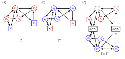
Figure 1: Gammoid representation of the input gramian. (a) An exemplary gammoid $\Gamma$. The nodes in red represent the input ground set $\mathcal{L}$ and the nodes in blue (squares) the output set $Z$. (b) The transposed gammoid $\Gamma^{\prime}$. Compared to (a), the arrows are flipped. The red nodes (squares) represent the input ground set $Z^{\prime}$ and the nodes in blue the output set $\mathcal{L}^{\prime}$. (c) The combined gammoid $(\Gamma\circ\Gamma^{\prime})$. The outputs $Z$ of $\Gamma$ are identified with the inputs $Z^{\prime}$ of $\Gamma^{\prime}$. Again, red nodes represent the inputs $\mathcal{L}$ and the blue nodes represent the outputs $\mathcal{L}^{\prime}$ of the gammoid $(\Gamma\circ\Gamma^{\prime})$.

Definition 8

Let $\Gamma$ be a weighted gammoid with ground set $\mathcal{L}=\{l_{1},\ldots,l_{L}\}$. For two nodes $l_{i},l_{j}\in\mathcal{L}$ let $\psi_{ij}$ denote the shortest path from $l_{i}$ to $l_{j}^{\prime}$ in $(\Gamma\circ\Gamma^{\prime})$. We call

$$\mu_{ij}^{\text{short}}:=\frac{|F(\psi_{ij})|}{\sqrt{F(\psi_{ii})F(\psi_{jj})}}$$ (18)

the shortest path coherence between $l_{i}$ and $l_{j}$.

Theorem 4

We find that

$$\mu_{ij}^{\text{short}}\geq\lim_{|s|\to\infty}\frac{|G_{ij}(s)|}{\sqrt{G_{ii}(s)G_{jj}(s)}}\,.$$ (19)

We see that

$$\inf_{s\in\mathbb{C}}\max_{i\neq j}\mu_{ij}(s)\leq\max_{i\neq j}\mu_{ij}^{\text{short}}$$ (20)

and therefore the shortest path mutual coherence can also be used in theorem 3 to get a (more pessimistic) bound for the spark. The advantage of the shortest path mutual coherence is that it can readily be computed even for large ($N>100$) networks.

3.4 Convex optimization for invariable sparse input reconstruction

As in compressed sensing for matrices, finding the solution of  (3) with a minimum number of non-zero components $\|{\mbox{$w$}}\|_{0}$ is an NP-hard combinatorial problem. Here, we formulate a convex optimal control problem as a relaxed version of this combinatorial problem. We define a Restricted-Isometry-Property (RIP) [20] for the input-output operator $\Phi$ defined by (1) and provide conditions for the exact recovery of invariable sparse errors in linear dynamic systems by solutions of the relaxed problem. As a first step it is necessary to introduce a suitable norm promoting invariable sparsity of the vector of input functions ${\mbox{$w$}}(t)$.

Say, $\mathcal{L}$ is an input ground set of size $L$. The space of input functions

$$\mathcal{W}:=\bigoplus_{i\in\mathcal{L}}\mathcal{W}_{i}$$ (21)

is composed of all function spaces $\mathcal{W}_{i}$ corresponding to input component $w_{i}$. Assume that each function space $\mathcal{W}_{i}=L^{p}([0,T])$ is a Lebesgue space equipped with the $p$-norm

$$\|w_{i}\|_{p}=\left(\int_{0}^{T}|w_{i}(t)|^{p}dt\right)^{1/p}\,.$$ (22)

We indicate the vector

$$\underline{{\mbox{$w$}}}:=\begin{pmatrix}\|w_{1}\|_{p}\\ \vdots\\ \|w_{L}\|_{p}\end{pmatrix}\,\in\mathbb{R}^{L}$$ (23)

collecting all the component wise function norms by an underline. Taking the $q$-norm in $\mathbb{R}^{L}$

$$\|\underline{{\mbox{$w$}}}\|_{q}=\left(\underline{w}_{1}^{q}+\ldots+\underline{w}_{L}^{q}\right)^{1/q}$$ (24)

of $\underline{{\mbox{$w$}}}$ yields the $p$-$q$-norm on $\mathcal{W}$

$$\|{\mbox{$w$}}\|_{q}:=\|\underline{{\mbox{$w$}}}\|_{q}\,.$$ (25)

The parameter $p$ appears implicitly in the underline. Since our results are valid for all $p\in[1,\infty)$, we will suppress it from the notation.

Similarly, for the $P$ outputs of the system, the output space

$$\mathcal{Y}=\mathcal{Y}_{1}\oplus\ldots\oplus\mathcal{Y}_{P}$$ (26)

can be equipped with a $p$-$q$-norm

$$\|{\mbox{$y$}}\|_{q}:=\|\underline{{\mbox{$y$}}}\|_{q}\,.$$ (27)

An important subset of the input space $\mathcal{W}$ is the space $\Sigma_{k}$ of invariable $k$-sparse inputs

$${\mbox{$w$}}\in\Sigma_{k}\Rightarrow\|{\mbox{$w$}}\|_{0}\leq k\,.$$ (28)

In analogy to a well known property [20] from compressed sensing we define for our dynamic problem:

Definition 9

The Restricted-Isometry-Property (RIP) of order $2k$ is fulfilled, if there is a constant $\delta_{2k}\in(0,1)$ such that for any two vector functions ${\mbox{$u$}},{\mbox{$v$}}\in\Sigma_{k}$ the inequalities

$$(1-\delta_{2k})\|\underline{{\mbox{$u$}}}-\underline{{\mbox{$v$}}}\|_{2}^{2}\leq\|\underline{\Phi({\mbox{$u$}})}-\underline{\Phi(\vec{v})}\|^{2}_{2}$$ (29)

and

$$\|\underline{\Phi({\mbox{$u$}})}+\underline{\Phi({\mbox{$v$}})}\|^{2}_{2}\leq(1+\delta_{2k})\|\underline{{\mbox{$u$}}}+\underline{{\mbox{$v$}}}\|_{2}^{2}$$ (30)

hold.

The RIP is well established in the literature on compressed sensing for finite dimensional maps [20, 38, 19, 35]. For this matrix case, bounds for the constants $\delta_{2k}$, [39] were derived and the null space property was formulated, see for instance [40] for recent work on a robust null space property. Connections to the mutual coherence also exist, see [34], where the mutual coherence inequality is investigated as an alternative to the RIP and where it was argued that in practical contexts such alternatives might be easier to handle. Our results on the newly defined coherence and RIP show that these notions are useful in the treatment of model errors of a dynamic system. It is currently an open question, whether it is possible to draw an analogous connection for our function space setting. Note that the structure of the input space $\mathcal{W}$ as a direct sum of Banach spaces makes the introduction of the underline (23) necessary. The underline, however, is a nonlinear operation. As a consequence, even for linear systems it is not obvious whether such a one-to-one analogy between compressed sensing for matrices and for dynamic systems can be established.

The reconstruction of invariable sparse unknown inputs can be formulated as the optimization problem

$$\text{minimize }\|{\mbox{$w$}}\|_{0}\text{ subject to }\|\Phi({\mbox{$w$}})-{\mbox{$y$}}^{\text{data}}\|_{2}\leq\epsilon$$ (31)

where $\epsilon>0$ incorporates uniform bounded measurement noise. A solution $\hat{{\mbox{$w$}}}$ of this problem will reproduce the data ${\mbox{$y$}}^{\text{data}}$ according to the dynamic equations (1) of the system with a minimal set of nonzero components, i.e., with a minimal set $S$ of input nodes. As before, finding this minimal input set is a NP-hard problem. Therefore, let us consider the relaxed problem

$$\text{minimize }\|{\mbox{$w$}}\|_{1}\text{ subject to }\|\Phi({\mbox{$w$}})-{\mbox{$y$}}^{\text{data}}\|_{2}\leq\epsilon\,.$$ (32)

The following result implies that for a linear system of ODEs with ${\mbox{$f$}}({\mbox{$x$}})=A{\mbox{$x$}}$ and ${\mbox{$c$}}({\mbox{$x$}})=C{\mbox{$x$}}$ with matrices $A\in\mathbb{R}^{N\times N}$ and $C\in\mathbb{R}^{P\times N}$ in (1) the optimization problem (32) has a unique solution.

Theorem 5

If $\Phi$ is linear, then (32) is a convex optimization problem.

For a given input vector ${\mbox{$w$}}\in\mathcal{W}$ we define the best invariable $k$-sparse approximation in $q$-norm as [19]

$$\sigma_{k}({\mbox{$w$}})_{q}:=\min_{{\mbox{$u$}}\in\Sigma_{k}}\|{\mbox{$w$}}-{\mbox{$u$}}\|_{q}\,,$$ (33)

i.e., we search for the function $u$ that has minimal distance to the desired function $w$ under the condition that $u$ has at most $k$ non-vanishing components. If $w$ is invariable $k$-sparse itself, then we can choose ${\mbox{$u$}}={\mbox{$w$}}$ and thus the distance between the approximation and the desired function vanishes, $\sigma_{k}({\mbox{$w$}})_{q}=0$.

Theorem 6

Assume $\Phi$ is linear and the RIP of order $2k$ holds. Let ${\mbox{$w$}}^{*}$ be the solution of (31). The optimal solution $\hat{{\mbox{$w$}}}$ of (32) obeys

$$\|\hat{{\mbox{$w$}}}-{\mbox{$w$}}^{*}\|_{2}\leq C_{0}\frac{\sigma_{k}({\mbox{$w$}}^{*})_{1}}{\sqrt{k}}+C_{2}\epsilon$$ (34)

with non-negative constants $C_{0}$ and $C_{2}$.

It is known, see for instance [19] that problem (32) can be reformulated via the cost functional

$$J[{\mbox{$w$}}]:=\frac{1}{2}\|\Phi({\mbox{$w$}})-{\mbox{$y$}}^{\text{data}}\|_{2}^{2}+\beta\|{\mbox{$w$}}\|_{1}$$ (35)

with given data ${\mbox{$y$}}^{\text{data}}$ and regularization constant $\beta$. The solution of the optimization problem in Lagrangian form

$$\text{minimize }J[{\mbox{$w$}}]\text{ subject to \eqref{eq:DynamicSystem}}\,,$$ (36)

provides an estimate for the input $\hat{{\mbox{$w$}}}$. Examples are be provided in the next section, see Fig. 2. A practical method to chose a suitable value for the regularisation parameter $\beta$ is the discrepancy method, see e.g. [41]. The basic idea is to increase $\beta$ up to the point where the data can not be fitted anymore to a given tolerance $\epsilon$. The tolerance can for example be inferred from the standard deviation of the measurement noise.

4 Numerical example for the reconstruction of an invariable sparse model error

In this section we illustrate by example, how our theoretical results from the previous section can be used to localize and reconstruct unknown inputs. These inputs can be genuine inputs from the environment or model errors or faults in a dynamic system [6, 7].

4.1 Error reconstruction in a linear dynamic system

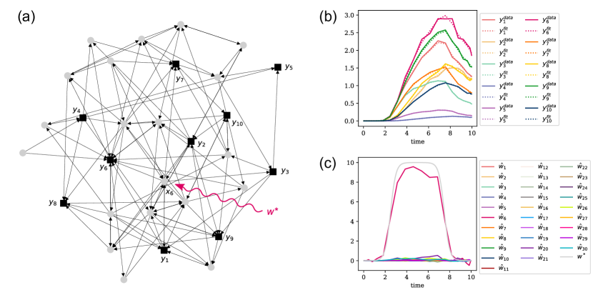
Figure 2: Reconstruction of an invariable sparse unknown input. (a) The influence graph of a linear dynamic system with $N=30$ states. The nodes correspond to the state variables and the edges indicate their interactions. The simulated error signal ${\mbox{$w$}}^{*}(t)=(0,\ldots,0,w_{6}^{*}(t),0,\ldots,0)^{T}$ targets the state variable $x_{6}$. The squares indicate the $P=10$ sensor nodes providing the output ${\mbox{$y$}}=(y_{1},\ldots,y_{10})^{T}$ (b) The measured output data ${\mbox{$y$}}^{\text{data}}(t)=(y^{\text{data}}_{1}(t),\ldots,y^{\text{data}}_{10}(t))^{T}$ (solid lines) can be fitted (dashed lines) by the output $\hat{{\mbox{$y$}}}(t)$ corresponding to the solution $\hat{{\mbox{$w$}}}(t)$ (see (c)) of the convex optimal control problem in (36). (c) This estimate $\hat{{\mbox{$w$}}}(t)$ simultaneously reconstructs the true unknown input ${\mbox{$w$}}^{*}(t)$. One can see that among the thirty inputs the node $i=6$ ($w_{6}$) was localized as the root cause of the error.

Assume, we have detected some unexpected output behaviour in a given dynamic system. Now, we want to reconstruct the root cause for the detected error. If the location of the state nodes would be known, then this would be a systems inversion problem [24, 25, 26, 7]. However, we assume here that we have no information about the location of the error. Thus, we need to reconstruct both the position of the states targeted by the error and its time course.

We simulated this scenario for a linear system with $N=30$ state nodes $\mathcal{N}=\{1,\ldots,30\}$ and randomly sampled the interaction graph $g$, see Fig.2(a). The outputs are given as time course measurements $y_{1}^{\text{data}}(t),\ldots,y_{10}^{\text{data}}(t)$ of $P=10$ randomly selected sensor nodes $Z$, see Fig.2(b). In our simulation, we have added the unknown input ${\mbox{$w$}}^{*}(t)$ with the only nonzero component $w^{*}_{6}(t)$ (Fig.2(c)). However, we assume that we have no information about the location of this unknown input. Thus, the ground set is $\mathcal{L}=\mathcal{N}$.

For a network of this size, it is still possible to exactly compute the spark (Definition 6) of the gammoid $(\mathcal{L},g,Z)$ (Definition 3). This straightforward algorithm iterates over two different loops: In the inner loop we iterate over all possible input sets $S$ of size $r$ and check, whether $S$ is linked in $g$ into $Z$ (see Theorem 1). In the outer loop we repeat this for all possible $r=1,2,\ldots,N$. The algorithm terminates, if we find an input set which is not linked into $Z$. If $r$ is largest subset size for which all $S$ are linked in $g$ into $Z$, the spark is given by $r+1$.

In larger networks, an exact computation of the spark can be too longsome. Then, we have to rely on the shortest path coherence (see definition 8) as an upper bound for the coherence (compare (20)).

For the network in  Fig.2(a) we find that $\text{spark}\,\Gamma=3$. From (8) we conclude that an unknown input targeting a single node in the network can uniquely be localized. Thus, under the assumption that the output residual was caused by an error targeting a single state node, we can uniquely reconstruct this input from the output. In this example, the shortest path mutual coherence $\max_{i\neq j}\mu_{ij}^{\text{short}}$ turns out to be equal to one and therefore leads to the bound $\text{spark}\,\Gamma\geq 2\,$. A spark of two, however, would mean that an unknown input on a single node can not be localized. This example illustrates that the shortest path coherence bounds on the spark and the error localizability can be quite conservative. This is the price to be paid for the much higher computational efficiency.

The reconstruction is obtained as the solution of the regularized optimization problem in (36), see Fig.2(c). For the fit we allowed each node $x_{i}$ to receive an input $\hat{w}_{i}$. We used a regularization constant of $\beta=0.01$ in  (36)) and $p=2$ for the components of the error (see (36)). The numerical solution was obtained by a discretisation of (36), see the Supplemental Text for an example program.

Please note that a necessary condition for the reconstruction to work is an assumption about the invariable $1$-sparsity of the unknown input. If we would assume that more than one state node is targeted by an error, we would need a larger spark to exactly localize and reconstruct the error. This would either require a smaller ground set $\mathcal{L}$ or a different set of sensor nodes $Z$, or both.

4.2 Recovering the nonlinearities of the chaotic Lorenz system

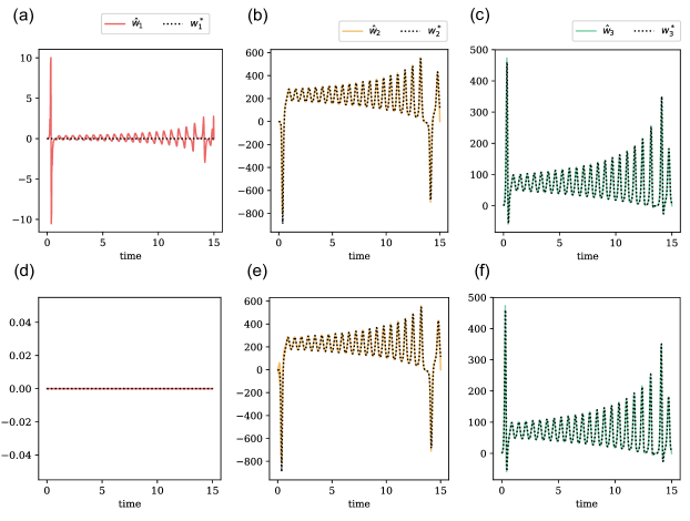
Figure 3: Reconstruction of the nonlinearities in the Lorenz system using the optimization based error reconstruction method (36). (a-c) The reconstructed error signals $\hat{{\mbox{$w$}}}=(\hat{w}_{1},\hat{w}_{2},\hat{w}_{3})^{T}$ when the linear system (38) is used as a model for the Lorenz system (37). The small signal $\hat{w}_{1}(t)$ for the first component suggests that this error could be neglected. (d-e) Constraining the first unknown input component to zero ($w_{1}=0$) still provides an accurate reconstruction of true error.

To illustrate that the reconstruction method (36) is also useful for nonlinear systems we considered the Lorenz system [42]

$$\dot{x}(t) =\sigma y(t)-\sigma x(t)$$ (37)

$$\dot{y}(t) =-x(t)y(t)+\rho x(t)-y(t)$$

$$\dot{z}(t) =x(t)y(t)-\beta z(t)\,,$$

with initial value $(x_{0},y_{0},z_{0})=(1,1,1)$ and the standard choice of parameters $\rho=28$, $\sigma=10$, and $\beta=8/3$.

Cancelling the nonlinearities of (37) we obtain

$$\dot{x}(t) =\sigma y(t)-\sigma x(t)$$ (38)

$$\dot{y}(t) =\rho x(t)-y(t)$$

$$\dot{z}(t) =-\beta z(t)\,.$$

Can we reconstruct the error incurred by this linear model using data from the "true system" (37)? We assumed that we can only measure variables $x$ and $z$ as output data from  (37).

The reconstructed error signal $\hat{{\mbox{$w$}}}$ and the true error ${\mbox{$w$}}^{*}$ are compared in Fig. 3(a-c). Clearly, the estimated signal $\hat{w}_{1}$ is small compared to the scale of the other components. This suggests a basic thresholding procedure were we set $w_{1}(t)=0$. Indeed, the reconstruction of the other components is still very accurate under this constraint, see Fig. 3(d-f).

Please note that the system (38) has a nonlinear, more precisely an affine input-output map $\Phi$. This suggests that the reconstruction method (36) can still be useful for nonlinear systems as well as nonlinear input-output maps, even if we have currently no proven accuracy bounds in the spirit of Theorem 6.

5 Discussion

Finding the root cause of errors or faults is important in many contexts. We have presented a mathematical theory for the localization of invariable sparse errors in ODE-models, which overcomes the need to a priori assume certain types of errors. This restriction is replaced by the invariable sparsity assumption, which is plausible in many real world settings, where the failure of a small number of components is observed from the sensors, but the localization of the fault is unknown. Similarly, for the problem of modelling dynamic systems, it is important to know where the model is wrong and which states in the model need a modified description. This includes also open systems, which are influenced by unknown inputs from their environment.

We have used the gammoid concept to define the notion of independence for inputs to dynamic systems. This allowed us to generalize concepts from sparse sensing to localize and recover such invariable sparse unknown inputs. Theorem 2 is general and applies to nonlinear systems. It is of note that Theorem 2 can also be used to test, how sparse the errors have to be in order to reconstruct their location for a given system with a given number of outputs. We are currently working towards a sensor node placement algorithm to relocate or add ouput measurements in order to increase the spark and therefore increase the number of error sources which can be localized with a minimum number of additional sensors.

The other results are only proved for linear systems. However, our numerical experiment with the Lorenz system suggests that the the optimization based recovery method in (32) is also suitable for highly nonlinear dynamics. In addition, the RIP-condition in Definition 9 is already hard to test for linear systems, a situation we already know from classical compressed sensing for matrices [18]. Thus, one important question for future research is a more operational criterion for the recovery of invariable sparse errors from solutions of the optimization problem (32) in linear and nonlinear systems in the presence of measurement errors.

There is a further complication in the problem of estimating the inverse of the input-output map $\Phi$ corresponding to the dynamic system (1): The map $\Phi$ is compact and maps from an infinite dimensional input space to the infinite dimensional output space. Inverse systems theory [33] tells us that the inversion of such operators is discontinous. Thus, more research on the numerics of this $L_{1}$-regularized estimation problem is needed [43]. Our results in Fig. 3 suggest that the idea of iterative thresholding [19] from classical compressed sensing can be transferred to our functional recovery problem. It will also be very intriguing to see, whether noniterative algorithms [44] can be designed for our dynamic system setting. In addition, stochastic dynamic systems with unknown inputs will provide another interesting direction for further research.

Our results are complementary to recent work on Data-Driven Dynamic Systems, where the the goal is to discover the dynamics solely from measurement data [45, 46, 47, 48]. For data sets of limited size, these purely data driven methods might be restricted to situations where all state variables are measured or time delays are used. In the more realistic case that not all the states can directly be measured, it might be useful to incorporate the prior knowledge encoded by a possibly imperfect but informative model. Our work suggests a promising approach to combine models and data driven methods: For a given model, the error signals should be estimated and then analysed with a data driven method to discover their inherent dynamics. In this way, the data driven method could be used to correct the informative but incomplete model. This could potentially decrease the number of measurements necessary in comparison to an ab initio, purely data driven model discovery approach. We believe that the combination of data driven systems with the prior information from interpretable mechanistic models will provide major advances in our understanding of dynamic networks.

References

- [1] R. Isermann, Fault-diagnosis applications. Heidelberg, Germany: Springer, 2011.
- [2] M. Blanke, M. Kinnaert, J. Lunze, and M. Staroswiecki, Diagnosis and Fault-Tolerant Control. Heidelberg, Germany: Springer, 2016.
- [3] D. J. Mook and J. L. Junkins, “Minimum model error estimation for poorly modeled dynamic systems,” Journal of Guidance, Control, and Dynamics, vol. 11, no. 3, pp. 256–261, May 1988.
- [4] J. Moreno, E. Rocha-Cozatl, and A. Vande Wouwer, “Observability/detectability analysis for nonlinear systems with unknown inputs - Application to biochemical processes,” in 2012 20th Mediterranean Conference on Control and Automation, MED 2012 - Conference Proceedings, Jul. 2012, pp. 151–156.
- [5] B. Engelhardt, H. Fröhlich, and M. Kschischo, “Learning (from) the errors of a systems biology model,” Scientific Reports, vol. 6, no. 20772, Nov. 2016. [Online]. Available: https://hal.archives-ouvertes.fr/hal-00152192
- [6] B. Engelhardt, M. Kschischo, and H. Fröhlich, “A Bayesian approach to estimating hidden variables as well as missing and wrong molecular interactions in ordinary differential equation-based mathematical models,” Journal of The Royal Society Interface, vol. 14, no. 131, p. 20170332, Jun. 2017.
- [7] D. Kahl, P. Wendland, M. Neidhardt, A. Weber, and M. Kschischo, “Structural Invertibility and Optimal Sensor Node Placement for Error and Input Reconstruction in Dynamic Systems,” Phys. Rev. X, vol. 9, no. 4, p. 041046, Dec. 2019.
- [8] M. Nagahara, D. E. Quevedo, and D. Nesic, “Maximum Hands-Off Control: A Paradigm of Control Effort Minimization,” IEEE Transactions on Automatic Control, vol. 61, no. 3, pp. 735–747, Mar. 2016.
- [9] T. Ikeda and K. Kashima, “On Sparse Optimal Control for General Linear Systems,” IEEE Transactions on Automatic Control, vol. 64, no. 5, pp. 2077–2083, May 2019.
- [10] M. Nagahara, D. Chatterjee, N. Challapalli, and M. Vidyasagar, “CLOT norm minimization for continuous hands-off control,” Automatica, vol. 113, p. 108679, Mar. 2020.
- [11] S. Sefati, N. J. Cowan, and R. Vidal, “Linear systems with sparse inputs: Observability and input recovery,” in 2015 American Control Conference (ACC). Chicago, IL, USA: IEEE, Jul. 2015, pp. 5251–5257.
- [12] M. Kafashan, A. Nandi, and S. Ching, “Analysis of Recurrent Linear Networks for Enabling Compressed Sensing of Time-Varying Signals,” arXiv:1408.0202 [math], Nov. 2015, [Preprint].
- [13] G. Joseph and C. R. Murthy, “Controllability of Linear Dynamical Systems Under Input Sparsity Constraints,” IEEE Transactions on Automatic Control, p. 1, Apr. 2020.
- [14] A. Olshevsky, “Minimal Controllability Problems,” IEEE Transactions on Control of Network Systems, vol. 1, no. 3, pp. 249–258, Sep. 2014.
- [15] Y.-Y. Liu and A.-L. Barabási, “Control principles of complex systems,” Reviews of Modern Physics, vol. 88, no. 3, p. 035006, Sep. 2016.
- [16] D. L. Donoho and M. Elad, “Optimally sparse representation in general (nonorthogonal) dictionaries via l1 minimization,” Proceedings of the National Academy of Sciences, vol. 100, no. 5, pp. 2197–2202, Mar. 2003.
- [17] D. L. Donoho, “Compressed sensing,” IEEE Transactions on Information Theory, vol. 52, no. 4, pp. 1289–1306, Apr. 2006.
- [18] Y. C. Eldar and G. Kutyniok, Compressed Sensing. Cambridge, UK: Cambridge University Press, 2012.
- [19] S. Foucart and H. Rauhut, A Mathematical Introduction to Compressive Sensing, ser. Applied and Numerical Harmonic Analysis. Cambridge, MA: Birkhauser Boston Inc., 2013.
- [20] E. Candes and T. Tao, “Decoding by linear programming,” IEEE Transactions on Information Theory, vol. 51, no. 12, pp. 4203–4215, Dec. 2005.
- [21] M. Kahm, C. Navarrete, V. Llopis-Torregrosa, R. Herrera, L. Barreto, L. Yenush, J. Ariño, J. Ramos, and M. Kschischo, “Potassium Starvation in Yeast: Mechanisms of Homeostasis Revealed by Mathematical Modeling,” PLoS Computational Biology, vol. 8, no. 6, pp. 1–11, Jun. 2012.
- [22] M. Schelker, A. Raue, J. Timmer, and C. Kreutz, “Comprehensive estimation of input signals and dynamics in biochemical reaction networks,” Bioinformatics, vol. 28, no. 18, pp. i529–i534, Sep. 2012.
- [23] N. Tsiantis, E. Balsa-Canto, and J. R. Banga, “Optimality and identification of dynamic models in systems biology: an inverse optimal control framework,” Bioinformatics, vol. 34, no. 14, pp. 2433–2440, Jul. 2018.
- [24] L. Silverman, “Inversion of multivariable linear systems,” IEEE Transactions on Automatic Control, vol. 14, no. 3, pp. 270–276, Jun. 1969.
- [25] M. Sain and J. Massey, “Invertibility of linear time-invariant dynamical systems,” IEEE Transactions on Automatic Control, vol. 14, no. 2, pp. 141–149, Apr. 1969.
- [26] M. Fliess, “A note on the invertibility of nonlinear input-output differential systems,” Systems & Control Letters, vol. 8, no. 2, pp. 147–151, Dec. 1986.
- [27] ——, “Nonlinear Control Theory and Differential Algebra: Some Illustrative Examples,” ser. 10th Triennial IFAC Congress on Automatic Control - 1987 Volume VIII, Munich, Germany, 27-31 July, vol. 20, no. 5, Part 8, Jul. 1987, pp. 103–107.
- [28] G. Basile and G. Marro, “A new characterization of some structural properties of linear systems: unknown-input observability, invertibility and functional controllability,” International Journal of Control, vol. 17, no. 5, pp. 931–943, May 1973.
- [29] T. Wey, “Rank and Regular Invertibility of Nonlinear Systems: A Graph Theoretic Approach,” IFAC Proceedings Volumes, vol. 31, no. 18, pp. 257–262, Jul. 1998.
- [30] H. Whitney, “On the Abstract Properties of Linear Dependence,” American Journal of Mathematics, vol. 57, no. 3, pp. 509–533, Jul. 1935.
- [31] H. Perfect, “Applications of Menger’s graph theorem,” Journal of Mathematical Analysis and Applications, vol. 22, no. 1, pp. 96–111, Apr. 1968.
- [32] J. S. Pym, “The Linking of Sets in Graphs,” Journal of the London Mathematical Society, vol. s1-44, no. 1, pp. 542–550, Jan. 1969.
- [33] G. Potthast and R. Nakamura, An introduction to the theory and methods of inverse problems and data assimilation. Bristol, UK: IOP Publishing, 2015.
- [34] T. T. Cai, L. Wang, and G. Xu, “Stable recovery of sparse signals and an oracle inequality,” IEEE Transactions on Information Theory, vol. 56, no. 7, pp. 3516–3522, 2010.
- [35] M. Vidyasagar, An Introduction to Compressed Sensing. SIAM - Society for Industrial and Applied Mathematics, 2019.
- [36] D. L. Donoho and P. B. Stark, “Uncertainty Principles and Signal Recovery,” SIAM Journal on Applied Mathematics, vol. 49, no. 3, pp. 906–931, Jun. 1989.
- [37] E. D. Sontag, “Mathematical Control Theory,” in Texts in Applied Mathematics, J. E. Marsden, L. Sirovich, M. Golubitsky, and W. Jäger, Eds., vol. 6. New York, NY: Springer New York, 1998.
- [38] Y. C. Eldar and G. Kutyniok, Eds., Compressed sensing: theory and applications. Cambridge ; New York: Cambridge University Press, 2012.
- [39] T. T. Cai and A. Zhang, “Sparse representation of a polytope and recovery of sparse signals and low-rank matrices,” IEEE Transactions on Information Theory, vol. 60, no. 1, pp. 122–132, 2014.
- [40] S. Ranjan and M. Vidyasagar, “Tight performance bounds for compressed sensing with conventional and group sparsity,” IEEE Transactions on Signal Processing, vol. 67, no. 11, pp. 2854–2867, 2019.
- [41] J. Honerkamp and J. Weese, “Tikhonovs regularization method for ill-posed problems: A comparison of different methods for the determination of the regularization parameter,” Continuum Mechanics and Thermodynamics, vol. 2, no. 1, pp. 17–30, 1990. [Online]. Available: http://link.springer.com/10.1007/BF01170953
- [42] E. N. Lorenz, “Deterministic Nonperiodic Flow,” Journal of the Atmospheric Sciences, vol. 20, no. 2, pp. 130–141, Mar. 1963.
- [43] G. Vossen and H. Maurer, “OnL1-minimization in optimal control and applications to robotics,” Optimal Control Applications and Methods, vol. 27, no. 6, pp. 301–321, Nov. 2006.
- [44] M. Lotfi and M. Vidyasagar, “A fast noniterative algorithm for compressivesensing using binary measurement matrices,” IEEE Transactions on Signal Processing, vol. 66, no. 15, pp. 4079–4089, 2018.
- [45] S. L. Brunton, J. L. Proctor, and J. N. Kutz, “Discovering governing equations from data by sparse identification of nonlinear dynamical systems,” Proc Natl Acad Sci USA, vol. 113, no. 15, pp. 3932–3937, Apr. 2016. [Online]. Available: http://www.pnas.org/lookup/doi/10.1073/pnas.1517384113
- [46] O. Yair, R. Talmon, R. R. Coifman, and I. G. Kevrekidis, “Reconstruction of normal forms by learning informed observation geometries from data,” Proc Natl Acad Sci USA, vol. 114, no. 38, pp. E7865–E7874, Sep. 2017.
- [47] J. Pathak, B. Hunt, M. Girvan, Z. Lu, and E. Ott, “Model-Free Prediction of Large Spatiotemporally Chaotic Systems from Data: A Reservoir Computing Approach,” Phys. Rev. Lett., vol. 120, no. 2, p. 024102, Jan. 2018.
- [48] K. Champion, B. Lusch, J. N. Kutz, and S. L. Brunton, “Data-driven discovery of coordinates and governing equations,” Proceedings of the National Acadameny of Sciences, vol. 116, no. 45, pp. 22 445–22 451, Nov. 2019.