Sparse image reconstruction on the sphere:
a general approach with uncertainty quantification

Abstract

Inverse problems defined naturally on the sphere are becoming increasingly of interest. In this article we provide a general framework for evaluation of inverse problems on the sphere, with a strong emphasis on flexibility and scalability. We consider flexibility with respect to the prior selection (regularization), the problem definition — specifically the problem formulation (constrained/unconstrained) and problem setting (analysis/synthesis) — and optimization adopted to solve the problem. We discuss and quantify the trade-offs between problem formulation and setting. Crucially, we consider the Bayesian interpretation of the unconstrained problem which, combined with recent developments in probability density theory, permits rapid, statistically principled uncertainty quantification (UQ) in the spherical setting. Linearity is exploited to significantly increase the computational efficiency of such UQ techniques, which in some cases are shown to permit analytic solutions. We showcase this reconstruction framework and UQ techniques on a variety of spherical inverse problems. The code discussed throughout is provided under a GNU general public license, in both C++ and Python.

I Introduction

Increasingly often one wishes to solve inverse problems natively on the sphere ($\mathbb{S}^{2})$ rather than on $n$ dimensional Euclidean space ($\mathbb{R}^{n})$, e.g. in astronomy and astrophysics [1, 2, 3], biomedical imaging [4, 5], and geophysics [6]. Straightforwardly from Gauss’ Theorema Egregium — which states that the curvature of surfaces embedded in $\mathbb{R}^{3}$ is immutable, and thus planar projections of curved manifolds (e.g. the sphere) inherently incur (significant) distortions — analysis over such domains must necessarily be conducted natively on the sphere. Though many Euclidean techniques may provide inspiration for counter-parts on the sphere, there are a still a great many critical differences between these paradigms which must be considered. Typically, inverse problems of interest, particularly on the sphere, are (often severely) ill-posed and/or ill-conditioned, motivating the injection of prior knowledge to stabilize the reconstruction. Such problems can be solved in a variety of ways (e.g. sampling methods and machine learning methods) though, for robustness and scalability, in the spherical setting variational methods (e.g. optimization) are the most effective.

Due to recent advances in the theory of compressed sensing [7, 8, 9] sparsity priors (e.g. $\ell_{1}$-regularization) are now routinely adopted, where the solution to an inverse problem can be constrained and found by promoting sparsity in a dictionary, such as wavelets or gradient space (variational norms). Recent developments in proximal convex optimization algorithms facilitate the practical application of non-differentiable priors, where they can be distributed and scale to high dimensional parameter spaces [10, 11]. The spherical counterparts for discrete gradient spaces [12], wavelet families [13, 14, 15], and scale-discretized wavelet families [16, 17, 18, 19, 20] have been developed, and have found wide applications — see previous papers in this series [12, 21] for a more comprehensive overview on this topic. Somewhat restricted investigations of some aspects have already been conducted, e.g. considering sparsity in spherical harmonic space [22], sparsity in various redundant dictionaries [23, 12, 21].

Variational inference techniques to solve inverse problems may be constructed in either the analysis or synthesis setting where signal coefficients or coefficients of a sparse representation are recovered respectively [24]. For Euclidean settings the analysis problem typically provides greater reconstruction fidelity; a characteristic often attributed to the lower cardinality of the analysis solution space [24, 25, 26], however comparisons between the analysis and synthesis settings on the sphere are not so clear, due to the approximate effective cardinality of different spaces on the sphere [21]. There also exists a more fundamental binary-classification of optimization problems: constrained and unconstrained, corresponding to regularization via hard and soft constraints respectively [27]. Hard constraints (constrained formulation) do not depend on variables such as Lagrangian multipliers, the optimal selection of which is an open problem, and instead constrain the solution to a certain sub-space. Soft constraints (unconstrained formulation) can be considered as Bayesian inference problems [28] and thus support a principled statistical interpretation [29, 30, 31].

Traditionally, although variational approaches may support a probabilistic interpretation they typically recover point estimates and do not quantify uncertainties. Fully probabilistic approaches (e.g. Markov chain Monte Carlo sampling methods) exist but are computationally expensive in the high dimensional setting of the sphere, motivating the development of hybrid techniques. Recent developments in the field of probability density theory [30] address precisely this consideration, facilitating flexible generation of scalable, fully principled Bayesian uncertainty quantification (UQ) techniques for variational approaches. Many such techniques have been developed [31, 32, 33, 34, 35], with applications in a variety of domains. In this article, we leverage these UQ techniques to recover Bayesian local credible intervals, in effect pixel-level error bars, and other forms of hypothesis tests on discrete spherical spaces. Interestingly we show how these uncertainties for a variety of common objectives can be computed rapidly (by exploiting linearity) and in some cases analytically. Such computational savings are a key component for the future of scalable UQ for spherical inverse problems. Looking forward one might note that these UQ techniques for variational imaging rely only on log-concavity of the posterior (convexity of the objective), as such a great many combinations of likelihood (data-fidelity) and prior (regularization functionals) are permissible.

In the spirit of open access software and scientific reproducibility the spherical reconstruction software (S2INV) developed during this project is made publicly available. S2INV is an object oriented C++ software package (with python extensions) which acts as a spherical extension to the SOPT [11, 36, 37] software package for flexible, efficient sparse optimization. We use fast exact spherical harmonic [38] and spherical wavelet transforms [17] to rapidly solve linear and ill-conditioned spherical inverse problems.

The remainder of this article is structured as follows. In Section II we provide the mathematical context which underpins analysis of spin signals on the sphere. In Section III we present variational regularization approaches to solve spherical inverse problems and consider the unconstrained and constrained formulations, in both the analysis and synthesis settings. Furthermore, we discuss the generalization of planar regularization functionals to their spherical counterparts, and briefly highlight highly optimized, scalable spherical reconstruction open-source software available as a bi-product of this work. In Section IV we develop principled Bayesian uncertainty quantification techniques which can be leveraged for spherical inverse problems, and present acceleration methods exploiting function linearity and/or objective analytic solutions. A diverse selection of numerical experiments are presented in Section V before providing concluding remarks in Section VI.

II Spin-signals on the sphere and rotation group

One often wishes to consider the frequency space representation of signals; whether this be embedded within regularization methods, necessary to fully capture a desired forward model, or simply adopted to exploit computational symmetries (e.g. fast convolution algorithms). In the Euclidean setting, the frequency information of a signal is efficiently expressed through projection onto Fourier space, the Fourier transform. For spherical settings frequency information is expressed though projection onto the space of spin spherical harmonics. In this section we review mathematical background fundamental to the analysis of signals defined on the sphere.

II-A Spin spherical harmonic transforms

The space of square integrable spin-$s$ functions ${}_{s}f\in\mathsf{L}^{2}[\mathbb{S}^{2}]$, for $s\in\mathbb{Z}$, with inner product $\langle\cdot|\cdot\rangle_{\mathbb{S}^{2}}$, are defined by their response under local rotations of $\chi\in[0,2\pi)$ about the tangent plane centered on the spherical co-ordinate $\omega=(\theta,\psi)\in\mathbb{S}^{2}$, given by ${}_{s}f^{\prime}(\omega)=\text{e}^{-is\chi}{}_{s}f(\omega)$ where ${}_{s}f^{\prime}$ is the rotated function [39, 40]. Such functions are most naturally represented by the spin-weighted spherical harmonics ${}_{s}Y_{\ell m}\in\mathsf{L}^{2}[\mathbb{S}^{2}]$ which are a set of complete and orthogonal basis functions for degree $\ell\in\mathbb{Z}^{+}$ and integer $m\in\mathbb{Z},\lvert m\rvert\leq\ell,\lvert s\rvert\leq\ell$. We adopt the Condon-Shortley phase convention [41], which results in conjugate symmetry ${}_{s}Y^{\star}_{\ell m}(\omega)=(-1)^{s+m}{}_{-s}Y_{\ell-m}(\omega)$, where $(\cdot)^{\star}$ denotes complex conjugation.

A spin-$s$ function ${}_{s}f\in\mathsf{L}^{2}[\mathbb{S}^{2}]$ may be decomposed into the spin spherical harmonic basis by

$${}_{s}f_{\ell m}\equiv\langle{}_{s}f_{\ell m}|{}_{s}Y_{\ell m}\rangle_{\mathbb{S}^{2}}=\int_{\mathbb{S}^{2}}d\Omega(\omega)\;{}_{s}f(\omega)\;{}_{s}Y_{\ell m}^{*}(\omega),$$ (1)

where $d\Omega(\omega)=\sin(\theta)d\theta d\psi$ is the standard rotation invariant measure (Haar measure) on the sphere. Equivalently, by the orthogonality and completeness of ${}_{s}Y_{\ell m}(\omega)$, one can exactly synthesize the signal space representation by

$${}_{s}f(\omega)=\sum^{\infty}_{\ell=0}\sum^{\ell}_{m=-\ell}{}_{s}f_{\ell m}\;{}_{s}Y_{\ell m}(\omega),$$ (2)

where the sum over $\ell$ is often truncated at $L$, where it is assumed that ${}_{s}f_{\ell m}=0,\forall\ell\geq L$. In this sense, signals are considered to be bandlimited at $L$. For notation brevity we adopt the shorthand operator notation $\bm{\mathsf{Y}}$ and $\bm{\mathsf{Y}}^{-1}$ to denote the forward and inverse spherical harmonic transforms.

This transformation allows one to probe the frequency content of spin signals defined on the sphere, which facilitates, e.g, efficient convolutions over spherical manifolds, in much the same way one can compute convolutions over $\mathbb{R}^{2}$ through the Fourier convolution theorem. In many cases signals have 0 spin, and so these relations collapse to the simpler form most readers are likely familiar with. Nevertheless, a variety of interesting physical settings exist where signals exhibit non-zero spin, e.g. weak gravitational lensing, the cosmic microwave background, or quantum mechanical systems.

II-B Scale-discretized directional spherical wavelets

Leveraging the above spin-$s$ spherical harmonic basis, and the associated convolutional properties, one can construct wavelet dictionaries naturally on the sphere. To do so one must first define a general rotation $\mathcal{R}_{\rho}$, for Euler angles $\rho=(\alpha,\beta,\gamma)\in\text{SO}(3)$ with $\alpha\in[0,2\pi),\beta\in[0,\pi)$, and $\gamma\in[0,2\pi)$, with action $(\mathcal{R}_{\rho}{}_{s}f)(\omega)\equiv e^{-is\theta}{}_{s}f(\mathcal{R}_{\rho}^{-1}\bm{\omega})$. The directional scale-discretized wavelet coefficients of any square integrable spin-$s$ function ${}_{s}f\in\mathsf{L}^{2}[\mathbb{S}^{2}]$ are given for scale $j$ by the directional convolution

$$W^{{}_{s}\Psi^{(j)}}(\rho) \equiv({}_{s}f\circledast{}_{s}\Psi^{(j)})(\rho)\equiv\langle{}_{s}f,\mathcal{R}_{\rho}{}_{s}\Psi^{(j)}\rangle_{\mathbb{S}^{2}}$$

$$=\int_{\mathbb{S}^{2}}d\Omega(\omega){}_{s}f(\omega)(\mathcal{R}_{\rho}{}_{s}\Psi^{(j)})^{\star}(\omega),$$ (3)

where $\circledast$ represents the directional spherical convolution and ${}_{s}\Psi^{(j)}\in\mathsf{L}^{2}[\mathbb{S}^{2}]$ is the wavelet kernel at scale $j\in\mathbb{Z}^{+}$, which determines the compact support of a given wavelet scale [17].

Typically wavelet coefficients have negligible energy concentration over the low-frequency domain in harmonic space, hence a scaling function ${}_{s}\Upsilon\in\mathsf{L}^{2}[\mathbb{S}^{2}]$ is introduced [19, 4] with coefficients $W^{{}_{s}\Upsilon}\in\mathsf{L}^{2}[\mathbb{S}^{2}]$ defined by the axisymmetric convolution $\odot$ with a signal ${}_{s}f\in\mathsf{L}^{2}[\mathbb{S}^{2}]$ such that

$$W^{{}_{s}\Upsilon}(\omega) \equiv({}_{s}f\odot{}_{s}\Upsilon)(\omega)\equiv\langle{}_{s}f,\mathcal{R}_{\omega}{}_{s}\Upsilon\rangle_{\mathbb{S}^{2}}$$

$$=\int_{\mathbb{S}^{2}}d\Omega(\omega^{\prime}){}_{s}f(\omega^{\prime})(\mathcal{R}_{\omega}{}_{s}\Upsilon)^{\star}(\omega^{\prime})\,,$$ (4)

where $\mathcal{R}_{\omega}=\mathcal{R}_{(\psi,\theta,0)}$ is a simplification of $\mathcal{R}_{\rho}$. One can straightforwardly show that the pixel-space representation of signals may be exactly synthesized if, and only if, the wavelet admissibility condition holds (see e.g. [19]). There exist many functions which are admissible, e.g. spherical needlets [42], ridgelets [4] and curvelets [43], however in this work we choose adopt the directional scale-discretized wavelet harmonic space kernel [16, 20], For notational brevity we define operators $\bm{\mathsf{\Psi}}$ and $\bm{\mathsf{\Psi}}^{-1}$ for the synthesis and analysis wavelet transforms respectively, with corresponding adjoints operators $\bm{\mathsf{\Psi}}^{\dagger}$ and $(\bm{\mathsf{\Psi}}^{-1})^{\dagger}$ (for further details see, e.g., [21]).

III Generalized spherical imaging

Imaging inverse problems are found in countless areas of both science and industry; consequently a great wealth of effort has been spent developing signal processing, Bayesian inference and, more recently, machine learning techniques for solving such problems. However, these techniques have overwhelmingly been restricted to Euclidean settings, in large part due to their prevelance and relative simplicity.

As such, planar imaging benefits greatly from the flexibility such a dictionary of techniques affords, whereas techniques developed for non-Euclidean manifolds (e.g. the sphere) are comparatively rare. One might reasonably consider applying planar techniques to spherical settings, e.g. through the analysis of planar projections, however these fundamentally fall short [2] as a result of Gauss’ Theorema Egregium — a core concept of differential geometry, which dictates that one may not flatten a ball without incurring significant distortions. Nonetheless, one can certainly consider the development of analogous techniques defined natively on the sphere. Previously, the spherical total variation TV-norm was constructed [12], and the analysis and synthesis settings were compared in a spherical setting [21]. In this section we extend the discussion to include the constrained and unconstrained formulations, supported by a variety of proximal optimization algorithms, and a variety of regularization functionals.

On the sphere the setup of such imaging problems is as follows: consider the case in which one acquires complex measurements $\bm{y}\in\mathbb{C}^{M}$, which may or may not be natively on the sphere, but can be related to an estimated or true spherical signal $\bm{x}\in\mathbb{C}^{N_{\mathbb{S}^{2}}}$ through the linear mapping

$$\bm{\mathsf{\Phi}}\in\mathbb{C}^{M\times N_{\mathbb{S}^{2}}}:\bm{x}\in\mathbb{C}^{N_{\mathbb{S}^{2}}}\mapsto\bm{y}\in\mathbb{C}^{M},$$ (5)

commonly referred to as the measurement operator, which simulates measurement acquisition. Suppose observations are contaminated with stochastic noise $\bm{n}\in\mathbb{C}^{M}$ such that $\bm{y}=\bm{\mathsf{\Phi}}\bm{x}+\bm{n}$ which is classically ill-posed. Furthermore, when one considers that spherical observations are often incomplete, i.e. $|M|\ll|N_{\mathbb{S}^{2}}|$, such problem instances quickly become (seriously) ill-conditioned. A diverse set of techniques exist to solve such inverse problems. This article is primarily concerned with variational approaches, for which we develop uncertainty quantification techniques in Section IV. Variational approaches consider the inverse problem as a minimization problem over a chosen objective function, which is typically the combination of a data fidelity term and a regularization term — selected to stabilize reconstruction with a priori assumptions as to the nature of the problem instance. Given an objective function over which to minimize, one must make a variety of decisions regarding optimization formulation.

III-A Constrained and unconstrained optimization

Suppose one selects data-fidelity term $f(\bm{x})$ and regularization functional $g(\bm{x})$, then the unconstrained optimization problem has the Lagrangian formulation [27]

$$\bm{x}^{\star}=\operatorname*{argmin}_{\bm{x}\in\Omega}\big{\{}f(\bm{x})+\lambda g(\bm{x})\big{\}},$$ (6)

where $\Omega=\{\mathbb{C}^{N_{\mathbb{S}^{2}}}$, $\mathbb{R}^{N_{\mathbb{S}^{2}}}$, $\mathbb{R}^{N_{\mathbb{S}^{2}}}_{+}\}$, and the regularization parameter $\lambda\in\mathbb{R}^{+}$ is a Lagrangian multiplier that balances the relative contributions of the two functions to the objective. In effect $\lambda$ allows for a smooth re-weighting (soft constraint) of the solution space instead of the strict boundary (hard constraint) imposed in the constrained problem. When one formulates such optimizations in the unconstrained setting, the solution which minimizes the objective is in fact the maximum a posteriori (MAP) estimator $\bm{x}^{\star}=\bm{x}^{\text{MAP}}$.

Interestingly, it is well known that the unconstrained problem has direct links to Bayesian inference and supports a principled statistical interpretation. However, until recently such Bayesian interpretations have been restricted to point estimators and/or severely restricted objective functional forms. One can leverage recent advances in probability concentration theory [30] to develop unconstrained optimization techniques which support principled uncertainty quantification, as discussed in Section IV. Therefore, when considering spherical imaging problems, where Bayesian sampling methods are impractical, in scientific domains, where uncertainty quantification is a desirable feature, unconstrained optimization exhibits significant advantages. However, this advantage comes at the additional complexity of optimal selection of the regularization parameter $\lambda$. Popular methods for selection of $\lambda$ have adopted criteria such as: the Akaike information criterion (AIC) [44], Bayesian information criterion (BIC) [45], or Stein’s unbiased risk estimator (SURE) [46, 47] and others [48]. Optimal regularization parameter selection is still very much an open problem (for various reasons including bias vs variance considerations). In this work we adopt a recently developed hierarchical Bayesian inference approach [49] which treats the regularization parameter as a nuisance variable [28] over which a majorization-minimization algorithm marginalizes. Effectively this method produces automatic, somewhat robust $\lambda$ selection with a straightforward, natural Bayesian interpretation, facilitating principled uncertainty quantification.

Suppose instead that one is unwilling to accept a trade-off in either the data-fidelity or regularization functional, i.e. one requires that the data-fidelity is strictly below a given threshold, or that solutions belong to a restrictive sub-space of the regularization support or measurement operator. For such inverse problems, the problem instance is formulated as a constrained optimization problem, in which one function is minimized subject to the constraint that the other function belongs to some constrained set [27]. Here we consider the common form in which the regularization functional is minimized subject to the constraint that the solution belongs within a level-set of the data-fidelity term, i.e.

$$\bm{x}^{\star}=\operatorname*{argmin}_{\bm{x}\in\Omega}\big{\{}g(\bm{x})\big{\}}\quad s.t.\quad f(\bm{x})\leq\delta,$$ (7)

where $\delta$ is a specified threshold (defining an iso-contour or level-set) of the data-fidelity term, typically determined by the noise variance. This optimization restricts solutions to the sub-space $\bm{x}\in\mathcal{B}^{\delta}_{f}$ where $\mathcal{B}^{\delta}_{f}$ is the $f$-ball centered at $\bm{z}\in\Omega$ with radius $\delta$, i.e. $\mathcal{B}^{\delta}_{f}(\bm{z})\coloneqq\{\bm{x}:f(\bm{x})\leq\delta\}.$

This formulation of the constrained problem requires calibration of $\delta$ which can be computed from the estimated noise variance, and has a well defined interpretation. The calibration of additional Lagrangian multipliers (regularization parameters) is not required, hence the constrained setting is typically more straightforward to adopt. For many problem instances the constrained setting provides greater reconstruction fidelity, though this is likely to be problem dependent. In this sense the soft constraint adopted by the unconstrained setting (when selected appropriately) allows for bias to be traded for variance (and vice versa) and thus in particularly ill-posed problem instances, where the prior weighting is large (i.e. high bias situations), may produce estimates that are more accurate. Furthermore, the constrained problem does not have an associated or well defined posterior distribution over the latent space, prohibiting principled uncertainty quantification.

III-B Analysis and synthesis settings

Often one adopts regularization functions which are computed on projections of the image space, e.g. wavelet space, harmonic space, gradient space etc.. In such settings one can formulate optimization problems that consider the inverse problem latent space to be the image space or the projected space, giving rise to the analysis and synthesis formulations respectively. In this way one recovers solutions in pixel-space $\bm{x}^{\star}$ (analysis) or projected space $\bm{\alpha}^{\star}$, which are then inverted to form pixel-space estimates $\bm{x}^{\star}=\bm{\mathsf{\Psi}}\bm{\alpha}^{\star}$ (synthesis) [24, 25, 26].

This is most easily illustrated by considering a simple example. Consider the wavelet Lasso regression problem in the analysis form, i.e. an $\ell_{1}$ wavelet regularization functional $g_{\text{A}}(\bm{x})=\lVert\bm{\mathsf{\Psi}}^{-1}\bm{x}\rVert_{1}$ and an $\ell_{2}$ data-fidelity term $f_{\text{A}}(\bm{x})=\lVert\bm{\mathsf{\Phi}}\bm{x}-\bm{y}\rVert_{2}^{2}$. Clearly in the analysis formulation the optimization problems are precisely those given in Section III-A. However, in the synthesis settings the regularization functional takes the form $g_{\text{S}}(\bm{\alpha})=\lVert\bm{\alpha}\rVert_{1}$, while the data-fidelity term is given by $f_{\text{S}}(\bm{\alpha})=\lVert\bm{\mathsf{\Phi}}\bm{\mathsf{\Psi}}\bm{\alpha}-\bm{y}\rVert_{2}^{2}$. With these definitions the synthesis optimization problem reads in much the same way as those presented in Section III-A and, in fact, for situations in which the measurement operator is orthogonal, i.e. $\bm{\mathsf{\Psi}}^{-1}=\bm{\mathsf{\Psi}}^{\dagger}$, these formulations are equivalent. However, they have very different geometric properties when this is not the case [24, 25, 26]. Notice that we adopt overcomplete spherical wavelet transforms where $\bm{\mathsf{\Psi}}^{-1}\not=\bm{\mathsf{\Psi}}^{\dagger}$, and sampled spherical harmonic transforms which are not orthogonal, i.e. $\bm{\mathsf{Y}}^{-1}\not=\bm{\mathsf{Y}}^{\dagger}$ [12] — a notable difference to the discrete Fourier transform in Euclidean settings. Therefore on the sphere the analysis and synthesis settings are not equivalent, and often produce noticeably different results.

In practice the analysis setting has consistently been demonstrated to exhibit greater reconstruction fidelity, a feature attributed to the lower cardinality of the analysis solution space [24, 25, 26]. However, in previous work it was concluded that this characteristic may not generalized to the spherical setting [21]. In Section V we revisit this analysis and find that the variation in relative performance, both in terms of reconstruction fidelity and computational efficiency, of each setting is dependent on the problem instance under consideration. Therefore, flexibility with respect to reconstruction formulation supports development of scalable spherical imaging algorithms tailored for specific applications. In this work we discover that implicit bandlimiting is often a determining factor when one considers inverse problems on the sphere, which impacts the effective cardinality of the spaces considered. In this sense it is beneficial to either (i) adopt the synthesis setting in which signals are implicitly bandlimited during reconstruction or (ii) explicitly bandlimit the analysis setting, which is some settings can be computationally inefficient on the sphere. An example of such computational savings in the synthesis setting is demonstrated in Section V-C, where an iterative Wiener filtering approach is adopted. In this case the analysis/synthesis formulations require $6,2$ spherical harmonic transforms respectively.

III-C Regularization functionals on the sphere

Having discussed the variety of ways one may formulate and construct an optimization on the sphere, we should now consider spherical counterparts to common regularization functionals and how one can develop these for the spherical setting. Such regularization functionals include e.g. sparsity promoting $\lVert\cdot\rVert_{1}$ regularizers, typically in a sparsifying dictionary $\bm{\mathsf{\Psi}}$, which are often motivated by the theory of compressed sensing [9, 8, 7]; Gaussian $\lVert\cdot\rVert_{2}^{2}$ regularizers, which are often iterative implementations of harmonic Wiener filters [50, 51]; and spherical total-variation (TV) priors [12], which are effective for edge detection and segmentation tasks.

Most imaging problems exist in the discrete settings, and so depend on approximations to the underlying continuous $\ell_{p}$-norms. In spherical settings one often adopts equiangular sampling [38], which does not uniformly sample the continuous norms. Typically this results in disproportionate weight being applied to pixels located at the poles, due to progressing increased sampling density away from the equator. To account for this spherical (directional wavelet) counter-parts to the traditional norms are defined by

$${}_{\mathbb{S}^{2}}\!\lVert\bm{x}\rVert_{p}=\lVert\bm{w}\circ\bm{x}\rVert_{p}\Rightarrow{}_{\Psi}\!\lVert\bm{\alpha}\rVert_{p}=\big{(}\sum_{j}\sum_{n}{}_{\mathbb{S}^{2}}\!\lVert\bm{\alpha}_{j,n}\rVert_{p}^{p}\big{)}^{\frac{1}{p}},$$ (8)

respectively, where $\bm{w}\in\mathbb{S}^{2}$ is the corresponding map of reciprocal pixel areas on the sphere, $\circ$ is the Hadamard product, and $j,n\in\mathbb{Z}^{+}$ are wavelet scale and direction respectively. This reformulation provides a closer approximation to the underlying continuous $\ell_{p}$-norm on the sphere.

With these corrected norms one can straightforwardly consider, e.g., sparsity in spherical wavelet space ${}_{\Psi}\!\lVert\bm{\mathsf{\Psi}}^{\dagger}\bm{x}\rVert_{1}$. Such a generalization permits multi-resolution algorithms [17] resulting in wavelet scale projections of varying resolution, which provide a significant increase in computational efficiency, a fundamental bottleneck of variational methods on the sphere. In theory one could leverage the exact quadrature weights inherent to the underlying spherical sampling theorems [38], however in this work we find simple weights $\bm{w}_{j,n}$ which capture the pixel area to be sufficient.

III-D Efficient flexible imaging on the sphere

Variational approaches efficiently locate optimal solutions via iterative algorithms, which typically leverage $1^{\text{st}}$-order (gradient) information to navigate towards extremal values. Furthermore, for convex objectives, such algorithms permit strong guarantees of both convergence and the rate of convergence. Imaging problems often adopt non-differentiable regularization functionals (e.g. $\ell_{1}$-norms) for which proximal operators may be used to navigate the objective function, thus motivating proximal convex optimization algorithms.

Convex optimization algorithms require successive iterations to converge; as such, any operators evaluated must be efficient and precise, so as to facilitate accurate, scalable methods. These considerations are more pronounced when considering optimization over spherical manifolds, wherein underlying operators (e.g. spin-$s$ spherical harmonic transforms) scale poorly with dimension ($\propto\mathcal{O}(L^{3})$ in the best case scenario). Additionally, a large subset of optimization algorithms require adjoint $\dagger$ operators, which are often incorrectly approximated by their inverse operators, introducing unpredictable errors and breaking convergence guarantees. Furthermore, on the sphere one must also consider the weighting scheme presented in Section III-C, which can be incorporated into proximal optimization algorithms through; a direct operator that performs the weighting, or by weighting norms. To avoid additional complications (e.g. under certain norms weighting operators do not represent tight frames, necessitating additional sub-iterations) we simply weight the norms directly.

During this research we developed a highly optimized object oriented (OOP) C++ software framework (S2INV) which permits all the aforementioned flexibility. The equiangular sampling theorem on the sphere of [38] is adopted through the SSHT package, which permits fast and efficient spin-$s$ spherical harmonic transforms, whilst permitting machine precision computation. Additionally, we adopt optimized scale-discretized directional wavelets on the sphere [16, 18, 19] through the S2LET package [17, 21], which are optimally sampled and support machine precision synthesis. We leverage a recently developed, highly optimized C++ OOP sparse optimization framework SOPT [11, 36, 37], which facilitates a variety of proximal convex optimization algorithms, e.g. forward-backward [52, 53], primal dual [27, 54, 55], and the alternating direction method of multipliers [56], with appropriate modifications for the spherical setting. In this way S2INV provides a scalable, flexible, open-source software package, which is fully customizable and supports a wide variety of novel, fully principled, uncertainty quantification techniques on the sphere, which we discuss in Section IV.

IV Spherical Bayesian uncertainty quantification

The unconstrained reconstruction problem has a straightforward Bayesian interpretation which is as follows. The posterior distribution of a spherical image $\bm{x}\in\mathbb{C}^{N_{\mathbb{S}^{2}}}$ defined over, e.g., the celestial sphere or the globe, given observations $\bm{y}\in\mathbb{C}^{M}$ is given by Bayes’ theorem,

$$P(\bm{x}|\bm{y};\mathcal{M})\equiv\frac{P(\bm{y}|\bm{x};\mathcal{M})P(\bm{x};\mathcal{M})}{\int_{\mathbb{C}^{N_{\mathbb{S}^{2}}}}P(\bm{y}|\bm{x};\mathcal{M})P(\bm{x};\mathcal{M})d\bm{x}},$$ (9)

where the likelihood encodes data fidelity, the prior encodes a priori information of the image, and $\mathcal{M}$ represents some model, which includes the mapping $\bm{\mathsf{\Phi}}\in\mathbb{C}^{M\times N_{\mathbb{S}^{2}}}:\bm{x}\mapsto\bm{y}$, and some understanding of the noise inherent to $\bm{y}$ [28]. Note that the marginal likelihood (Bayesian evidence) is a constant scaling of the posterior and can be used for model comparison, which we do not consider further in this article.

Typically sampling methods, e.g. Markov chain Monte Carlo, are adopted to sample from the posterior distribution from which one can determine a point estimation of the solution to the inverse problem and the distribution of uncertainty about such a solution. Although these methods recover asymptotically exact estimates of the posterior distribution, they typically require large numbers of samples to converge. Each sample requires at least a single evaluation of the posterior which in spherical settings is computationally demanding — for moderate resolutions $L>10^{3}$ sampling methods rapidly become computationally intractable.

Instead consider a variational approach that maximizes the posterior odds, referred to as the maximum a posteriori (MAP) solution defined by

$$\bm{x}^{\text{MAP}} \equiv\operatorname*{argmax}_{\bm{x}}\big{\{}P(\bm{x}|\bm{y};\mathcal{M})\big{\}},$$

$$\propto\operatorname*{argmin}_{\bm{x}}\big{\{}-\log(\;P(\bm{y}|\bm{x};\mathcal{M})P(\bm{x};\mathcal{M})\;)\big{\}},$$

$$\propto\operatorname*{argmin}_{\bm{x}}\big{\{}h(\bm{x})=f(\bm{x})+g(\bm{x})\big{\}},$$ (10)

where the second line follows by the monotonicity of the logarithm function. For convex objective functions $h(\bm{x})$ this takes the form of a convex optimization problem [27], and therefore Equation 6 explicitly returns the MAP solution, as asserted in Section III-A. Hence, leveraging state-of-the-art convex optimization techniques one can efficiently locate the solution which maximizes the posterior odds. However this is still a point estimate which, though useful, does not naively support uncertainty quantification. Recently, approximate contours of the latent space have been derived facilitating variational regularization methods with principled uncertainty quantification. We discuss these approximate methods and develop uncertainty quantification techniques on the sphere, which we accelerate by exploiting function linearity.

IV-A Highest posterior density credible regions

A credible region $C_{\alpha}\subset\mathbb{C}^{N_{\mathbb{S}^{2}}}$ of the posterior latent space at credible confidence $100(1-\alpha)\%$, for $\alpha\in[0,1]$, satisfies the integral equation [28]

$$P(\bm{x}\in C_{\alpha}|\bm{y};\mathcal{M})=\int_{\bm{x}\in\mathbb{C}^{N_{\mathbb{S}^{2}}}}P(\bm{x}|\bm{y};\mathcal{M})\mathbb{I}_{C_{\alpha}}d\bm{x}=1-\alpha,$$ (11)

where $\mathbb{I}_{C_{\alpha}}$ is the standard set indicator function. The optimal credible region in the sense of minimal volume [28] is the highest posterior density (HPD) credible region defined by $C_{\alpha}\coloneqq\{\bm{x}:h(\bm{x})\leq\epsilon_{\alpha}\}$, where $\epsilon_{\alpha}\in\mathbb{R}^{+}$ is an isocontour of the log-posterior. Determination of the HPD region requires computation of the integral in Equation 11, which is computationally infeasible in even moderate dimensional spherical settings, due to dimensionality and functional complexity considerations. Convex objectives $h(\bm{x})$ support the conservative approximate HPD credible region $C^{\prime}_{\alpha}$ defined by [30]

$$C_{\alpha}\subseteq C^{\prime}_{\alpha}\subset\mathbb{C}^{N_{\mathbb{S}^{2}}} \coloneqq\Big{\{}\bm{x}:h(\bm{x})\leq\epsilon^{\prime}_{\alpha}\Big{\}},$$

$$\text{where}\quad\epsilon^{\prime}_{\alpha}=h(\bm{x}^{\text{MAP}}) +\sqrt{16N\log(3/\alpha)}+N,$$ (12)

which allows one to approximate $C_{\alpha}$ with only knowledge of the MAP solution $\bm{x}^{\text{MAP}}$ and the dimension $N=\mathbb{C}^{N_{\mathbb{S}^{2}}}$. An upper bound on the approximation error exists [30]. Therefore for convex objectives, given $\bm{x}^{\text{MAP}}$, one may draw statistically principled conclusions. This credible set approximation has been leveraged to develop fast Bayesian uncertainty quantification techniques in a variety of settings [31, 33, 34, 35, 32, 30].

IV-B Bayesian hypothesis testing on the sphere

The most straightforward uncertainty quantification technique one may generate by leveraging the approximation of Equation 12 is that of hypothesis testing [31, 33, 1]. The concept of hypothesis testing is to adjust a feature of the recovered estimator $\bm{x}^{\text{MAP}}$ generating a surrogate solution $\bm{x}^{\text{sur}}$, of which we ask $\bm{x}^{\text{sur}}\in C^{\prime}_{\alpha}$? If $\bm{x}^{\text{sur}}\not\in C^{\prime}_{\alpha}\Rightarrow\bm{x}^{\text{sur}}\not\in C^{\prime}$, which follows from the conservative nature of the approximation in Equation 12, the feature of interest is considered to be statistically significant (necessary to the reconstruction) at $100(1-\alpha)\%$ confidence. Conversely $\bm{x}^{\text{sur}}\in C^{\prime}_{\alpha}$ indicates that the surrogate solution remains within the approximate credible set and we conclude that the feature is indeterminate.

IV-C Local credible intervals on the sphere

Suppose one recovers an optimal solution $\bm{x}^{\text{MAP}}$ through unconstrained convex optimization (see Section III-A) and wishes to quantify the uncertainty associated with a given pixel or super pixel (collection of pixels). With knowledge of the approximate level set threshold $\epsilon^{\prime}_{\alpha}$, and therefore the approximate HPD credible set $C^{\prime}_{\alpha}$ at well defined confidence $(100-\alpha)\%$, one simply needs to iteratively compute the extremal values a given region of interest may take, such that the resulting solution falls outside of the approximate HPD credible set, i.e. $\bm{x}^{\text{sur}}\not\in C^{\prime}_{\alpha}$. One must then define which types of regions (super-pixels) on the sphere one is interested in.

Formally, select independent partitions of the latent space $\Omega=\cup_{i}\Omega_{i}$ for which we define super-pixel indexing functions $\zeta_{(\cdot)}$ such that $\bm{x}_{i}\in\Omega_{i}\Rightarrow\zeta_{\Omega_{i}}=1$ and $\bm{x}_{i}\notin\Omega_{i}\Rightarrow\zeta_{\Omega_{i}}=0$. For a given $\Omega_{i}$ locate upper (lower) bounds $\xi^{+}_{\Omega_{i}}$, $\xi^{-}_{\Omega_{i}}$ respectively, which saturate the HPD credible region $C^{\prime}_{\alpha}$ [31, 34]. This is achieved by the following optimizations,

$$\xi^{\pm}_{\Omega_{i}} =\operatorname*{max}_{\xi\in\mathbb{R}^{+}}\big{\{}\pm\xi|f(\bm{x}_{i,\xi})+g(\bm{x}_{i,\xi})\leq\epsilon^{\prime}_{\alpha}\big{\}},$$ (13)

where $\bm{x}_{i,\xi}=\bm{x}^{\text{MAP}}\zeta_{\Omega/\Omega_{i}}+\xi\zeta_{\Omega_{i}}$ is a surrogate solution where the super pixel region has been replaced by a uniform intensity $\xi$. The collective set of these bounds $\{\lvert\xi^{+}_{\Omega_{i}}-\xi^{-}_{\Omega_{i}}\rvert\}$ is taken to be the local credible interval map [31], which can simply be recovered via bisection. Though conditional local uncertainty quantification techniques such as this have demonstrated utility in certain circumstances [31, 33, 34, 35], in the high dimensional spherical settings they can quickly become dilute [1]. This makes intuitive sense, as small (local) objects (super-pixels) in high dimensional settings become statistically insignificant. As such, in high-dimensional spherical settings global or aggregate (statistical) uncertainty quantification techniques are often more meaningful (see e.g [1]).

IV-C1 Gridding schemes

One can construct rectangular partitions directly on the latent space (e.g. uniform gridding). However, in the spherical setting it is sometimes more meaningful to define a super pixel by a fixed physical area surrounding a defined central pixel. Practically this is computed as follows: define a central pixel on the sphere, rotate this pixel to a pole (where higher angular resolution provides greater fine tuning of super-pixel area), select a given angular deviation from the pole, define this spherical cap as the super pixel. In this way all super pixels are, by definition, of equal area.

IV-D Acceleration through linearity

Naive computation of local credible intervals through bisection can often require many evaluations of the objective function, which is particularly costly when one considers functions on the sphere. To avoid this computational bottleneck we exploit the linearity of such operators. Consider the generalized convex objective function for the analysis setting, without loss of generality, which can be written as

$$h(\bm{x})=f(\bm{x})+g(\bm{x})=\lVert\bm{\mathsf{\Phi}}\bm{x}-\bm{y}\rVert_{p_{1}}^{p_{2}}+\lVert\bm{\mathsf{\Psi}}^{\dagger}\bm{x}\rVert_{q_{1}}^{q_{2}}.$$ (14)

Consider again the partition $\bm{x}^{\text{sur}}=\bm{x}\zeta_{\Omega/\Omega_{i}}+\xi\zeta_{\Omega_{i}}$ upon which the applications of any linear operator $\mathcal{L}$ is given trivially by linearity to be $\bm{\mathcal{L}}\bm{x}^{\text{sur}}=\bm{\mathcal{L}}\bm{x}\mathbb{I}_{\zeta_{\Omega/\Omega_{i}}}+\xi\bm{\mathcal{L}}\mathbb{I}_{\zeta_{\Omega_{i}}}$. Explicitly expanding Equation 14 with linearity one finds

$$\lVert\bm{\mathsf{\Phi}}\bm{x}\mathbb{I}_{\zeta_{\Omega/\Omega_{i}}}+\xi\bm{\mathsf{\Phi}}\mathbb{I}_{\zeta_{\Omega_{i}}}-\bm{y}\rVert^{p_{2}}_{p_{1}} +\lVert\bm{\mathsf{\Psi}}^{\dagger}\bm{x}\mathbb{I}_{\zeta_{\Omega/\Omega_{i}}}+\xi\bm{\mathsf{\Psi}}^{\dagger}\mathbb{I}_{\zeta_{\Omega_{i}}}\rVert^{q_{2}}_{q_{1}},$$

$$\Rightarrow\lVert\bm{a}+\xi\bm{b}\rVert^{p_{2}}_{p_{1}} +\lVert\bm{c}+\xi\bm{d}\rVert^{q_{2}}_{q_{1}},$$ (15)

for constant (per credible interval) vectors defined to be

$$\bm{a} =\bm{\mathsf{\Phi}}\bm{x}\mathbb{I}_{\zeta_{\Omega/\Omega_{i}}}-\bm{y} \quad\bm{b} =\bm{\mathsf{\Phi}}\mathbb{I}_{\zeta_{\Omega_{i}}}$$

$$\bm{c} =\bm{\mathsf{\Psi}}^{\dagger}\bm{x}\mathbb{I}_{\zeta_{\Omega/\Omega_{i}}} \quad\bm{d} =\bm{\mathsf{\Psi}}^{\dagger}\mathbb{I}_{\zeta_{\Omega_{i}}}$$ (16)

In this way the local credible optimization problems in Equation 13 can be re-written instead as

$$\lVert\bm{a}+\xi\bm{b}\rVert^{p_{2}}_{p_{1}}+\lVert\bm{c}+\xi\bm{d}\rVert^{q_{2}}_{q_{1}}\leq\epsilon^{\prime}_{\alpha},$$ (17)

which is clearly just a 1-dimensional polynomial root finding problem. One could approach this inequality from an iterative perspective, forming an upper bound through the Minkowski inequality, which is then leveraged as initialization for bisection. For polynomials of order $<5$ (see Abel-Ruffini theorem) Equation 17 permits analytic solutions. In practice the computational difference between the analytic solution and solving an inequality bounded bisection problem is marginal, though in high dimensions this speed up is non-negligible.

IV-D1 Gaussian regression

Suppose one adopts both a Gaussian likelihood and prior (e.g. iterative Wiener filtering approaches), in such a setting we have $p_{1}=p_{2}=q_{1}=q_{2}=2$ which reduces Equation 17 to the binomial inequality $\lVert\bm{a}+\xi\bm{b}\rVert^{2}_{2}+\lVert\bm{c}+\xi\bm{d}\rVert^{2}_{2}\leq\epsilon^{\prime}_{\alpha}$, which expands to give

$$\big{[}\lVert\bm{b}\rVert_{2}^{2}+\lVert\bm{d}\rVert_{2}^{2}\big{]}\xi^{2}+2\big{[}\bm{a}\cdot\bm{b}+\bm{c}\cdot\bm{d}\big{]}\xi+\big{[}\lVert\bm{a}\rVert_{2}^{2}+\lVert\bm{c}\rVert_{2}^{2}\big{]}\leq\epsilon^{\prime}_{\alpha}.$$ (18)

One could gain some geometric insight by considering the case in which $\bm{a}\cdot\bm{b}+\bm{c}\cdot\bm{d}=0$, as in such a case the resulting credible region about the posterior is symmetric, however we do not consider this further here. Nonetheless, per credible region the interval is trivially recovered.

IV-D2 Lasso regression

Consider the Lagrangian dual of the Lasso regression (e.g. sparse reconstruction), in which we have $p_{1}=p_{2}=2$ and $q_{1}=q_{2}=1$, such that the general polynomial Equation 17 reduces to a $2^{\text{nd}}$-order polynomial $\lVert\bm{a}+\xi\bm{b}\rVert^{2}_{2}+\lVert\bm{c}+\xi\bm{d}\rVert_{1}\leq\epsilon^{\prime}_{\alpha}$, which, assuming the intersection of the partitions projected into $\bm{\mathsf{\Psi}}$ is negligible, i.e. the dictionary $\bm{\mathsf{\Psi}}$ has sufficient localization properties on the sphere, results in the inequality

$$\lVert\bm{b}\rVert_{2}^{2}\xi^{2}+2\big{[}\bm{a}\cdot\bm{b}+\lVert d\rVert_{1}\big{]}\xi+\big{[}\lVert\bm{a}\rVert_{2}^{2}+\lVert\bm{c}\rVert_{1}\big{]}\leq\epsilon^{\prime}_{\alpha},$$ (19)

which can be analytically solved. Typically the partitions $\Omega_{i}$ projected into $\bm{\mathsf{\Psi}}$ exhibit overlapping support and so this inequality is not exact. In such cases one can perform bisection, computing only the $\ell_{1}$ term at each iteration.

V Numerical experiments

In this section we showcase the variational regularization and uncertainty quantification techniques presented in Section III and Section IV on a diverse set of numerical experiments. For each scenario we create mock observations $\bm{y}=\bm{\mathsf{\Phi}}\bm{x}$ of a ground truth signal $\bm{x}$ which are related through the forward model $\bm{\mathsf{\Phi}}:\bm{x}\mapsto\bm{y}$ from which we formulate an ill-posed inverse problem (e.g. add noise, mask, blur, etc.). We solve this inverse problem for an estimator $\bm{x}^{\star}$ ($\bm{x}^{\text{MAP}}$) of $\bm{x}$ the success of which we quantify by the recovered signal to noise ratio, defined by $\text{SNR}=20\log_{10}({\lVert\bm{x}\rVert_{2}}/{\lVert\bm{x}-\bm{x}^{\star}\rVert_{2}})$.

V-A Earth satellite topography

Suppose a satellite performs observations $\bm{y}\in\mathbb{R}^{M}$ of the Earth’s topography (geographic elevation) which can be related to the true topography $\bm{x}\in\mathbb{R}^{N_{\mathbb{S}^{2}}}$ through a mapping (forward model) $\bm{\mathsf{\Phi}}_{\text{ET}}\in\mathbb{R}^{M\times N_{\mathbb{S}^{2}}}:\bm{x}\mapsto\bm{y}$. Consider the scenario in which incomplete, i.e. $\lvert M\rvert\ll\lvert N_{\mathbb{S}^{2}}\rvert$, observations $\bm{y}$ are contaminated with independent and identically distributed (i.i.d.) Gaussian noise $\bm{n}\sim\mathcal{N}(0,\sigma^{2})\in\mathbb{R}^{M}$, and blurred with an axisymmetric smoothing kernel with full width half maximum (FWHM) $\Theta$. In such a case observations are modeled by $\bm{y}=\bm{\mathsf{\Phi}}_{\text{ET}}\bm{x}+\bm{n}$ for measurement operator

$$\bm{\mathsf{\Phi}}_{\text{ET}}=\bm{\mathsf{D}}\bm{\mathsf{Y}^{-1}}\bm{\mathsf{\Theta}}\bm{\mathsf{Y}}\quad\text{and}\quad\bm{\mathsf{\Phi}}_{\text{ET}}^{\dagger}=\bm{\mathsf{Y}}^{\dagger}\bm{\mathsf{\Theta}}\ (\bm{\mathsf{Y}}^{-1})^{\dagger}\bm{\mathsf{D}}^{\dagger},$$ (20)

where $\bm{\mathsf{Y}},\bm{\mathsf{Y}}^{-1}$ are forward and inverse spherical harmonic transforms correspondingly, $\bm{\mathsf{D}},\bm{\mathsf{D}}^{\dagger}$ are masking and projection operators correspondingly, $\bm{\mathsf{\Theta}}$ is the axisymmetric convolution with the harmonic representation of $\Theta$ which is trivially self-adjoint, and $\dagger$ represents the adjoint operation.

As $\bm{n}$ is a univariate Gaussian the data-fidelity (log-likelihood) term is simply given by $\frac{1}{2\sigma^{2}}{}_{\mathbb{S}^{2}}\!\lVert\bm{\mathsf{\Phi}}_{\text{ET}}\bm{x}-\bm{y}\rVert_{2}^{2}$. Here we adopt a sparsity promoting $\ell_{1}$-norm wavelet regularization ${}_{\Psi}\!\lVert\bm{\mathsf{\Psi}}^{\dagger}(\cdot)\rVert_{1}$ (Laplace distribution log-prior), and solve both the constrained formulation through the proximal ADMM algorithm [56] and the unconstrained formulation through the proximal forward backward algorithm [53, 52, 27], in both the analysis and synthesis settings. Notice the use of spherical (wavelet) space norms, outlined in Section III-C, which better approximate spherical continuous norms.

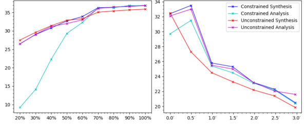
Figure 1: Left: Recovered SNR for a variety of problem setups over a variety of inpainting scenarios versus % of pixels observed. Right: Recovered SNR for a variety of problem setups versus variety of axisymmetric blurring kernel scales, for a fixed inpainting of 50% masked pixels. Discussion: Generally each setup performs similarly and it would appear that no single setting is optimal in all cases. Notice the drastic underperformance of the analysis constrained formulation in the heavily masked regime for the inpainting problem. We find that this asymmetry is due to the implicit spherical harmonic bandlimiting inherent to the synthesis problem (see text).

To quantify the impact of analysis versus synthesis (and constrained versus unconstrained) settings we consider all settings in two paradigms (i) varying levels of inpainting without deconvolution (ii) varying scales of deconvolution with 50% masked pixel inpainting. Generally, each problem setup performs comparably in all settings considered (see Figure 1). Certainly it cannot be said that one reconstruction paradigm is optimal in all settings, which leads us to conclude that it is likely that problem formulation optimality is ambiguous and should be selected on a case by case basis. Interestingly, notice the underperformance of the constrained analysis problem in the heavily masked regime (see the left plot of Figure 1). This was observed in prior analysis [21] and reported as evidence that the synthesis setting may produce more optimal results.

Note that the synthesis setting implicitly bandlimits the observations $\bm{x}$, therefore restricting the solution space cardinality — a factor known to impact reconstruction fidelity [24]. To account for this bias we reran the analysis optimization with an explicitly bandlimited measurement operator, results of which can be seen in Figure 3 (which also demonstrates the uncertainty quantification of Section IV-C). It was found that the analysis setting performs similarly to the synthesis setting for this problem, leading us to conclude that the optimality of optimization formulation is at best ambiguous.

Figure 2: Left: Simulated observations contaminated with 30dB Gaussian i.i.d. noise, convolved with a $\sim 268$ arc-minute Gaussian blurring kernel, and with 60% of pixels masked. Right: Unconstrained reconstruction using $\ell_{1}$-norm wavelet sparsity regularization (log-prior) in the analysis setting, adopting the proximal forward-backward algorithm [53, 27, 52]. Bottom: Bayesian local credible intervals at $99\%$ confidence (reconstruction values are $\in[-1,1]$), which are pixel-level uncertainties (see Section IV).

Figure 3: Left: Simulated observations contaminated with 30dB Gaussian noise and convolved with a $\sim 78$ arc-minute Gaussian blurring kernel (e.g. motion blur). Right: Spherical TV-norm $\lVert\bm{x}\rVert_{\text{TV}}$ regularized reconstruction through proximal primal dual algorithm in the analysis setting.

V-B $360^{\circ}$ camera blur deconvolution

Suppose a $360^{\circ}$ camera captures a greyscale spherical image $\bm{y}\in\mathbb{R}^{M_{\mathbb{S}^{2}}}$ which can be related to the true image $\bm{x}\in\mathbb{R}^{N_{\mathbb{S}^{2}}}$ through the forward model $\bm{\mathsf{\Phi}}_{360^{\circ}}\in\mathbb{R}^{M_{\mathbb{S}^{2}}\times N_{\mathbb{S}^{2}}}:\bm{x}\mapsto\bm{y}$. Consider that the camera captures complete $\lvert M_{\mathbb{S}^{2}}\rvert=\lvert N_{\mathbb{S}^{2}}\rvert$ observations but introduces low-level i.i.d. Gaussian noise $\bm{n}\sim\mathcal{N}(0,\sigma^{2})\in\mathbb{R}^{M_{\mathbb{S}^{2}}}$ and a certain amount of lens blurring characterized by axisymmetric convolution with a Gaussian smoothing kernel with FWHM = $\Theta$. In this case observations are modeled by $\bm{y}=\bm{\mathsf{\Phi}}_{360^{\circ}}\bm{x}+\bm{n}$ for measurement operator

$$\bm{\mathsf{\Phi}}_{360^{\circ}}=\bm{\mathsf{Y}}^{-1}\bm{\mathsf{\Theta}}\bm{\mathsf{Y}}\quad\text{and}\quad\bm{\mathsf{\Phi}}_{360^{\circ}}^{\dagger}=\bm{\mathsf{Y}}^{\dagger}\bm{\mathsf{\Theta}}\ (\bm{\mathsf{Y}}^{-1})^{\dagger},$$ (21)

where $\bm{\mathsf{Y}},\bm{\mathsf{Y}}^{-1}$ are forward and inverse spherical harmonic transforms correspondingly (see section II), $\bm{\mathsf{\Theta}}$ is the axisymmetric convolution with the harmonic representation of $\Theta$.

As in the previous example the data-fidelity is given by the ${}_{\mathbb{S}^{2}}\!\lVert\bm{\mathsf{\Phi}}_{360^{\circ}}\bm{x}-\bm{y}\rVert_{2}^{2}$. Depending on the degree to which $\bm{x}$ is piece-wise constant the TV-norm ${}_{\mathbb{S}^{2}}\!\lVert\bm{x}\rVert_{\text{TV}}={}_{\mathbb{S}^{2}}\!\lVert\nabla\bm{x}\rVert_{2}$ (promoting gradient sparsity) constitutes a good choice of regularizer. For image deconvolution an analysis wavelet sparsity promoting regularizer ${}_{\Psi}\!\lVert\bm{\mathsf{\Psi}}^{-1}\bm{x}\rVert_{1}$ is often also considered. Here we consider both regularization functionals $g(\bm{x})=\{{}_{\mathbb{S}^{2}}\!\lVert\bm{x}\rVert_{\text{TV}},{}_{\Psi}\!\lVert\bm{\mathsf{\Psi}}^{-1}\bm{x}\rVert_{1}\}$ in the constrained analysis setting:

$$\bm{x}^{\star}=\operatorname*{argmin}_{\bm{x}\in\mathbb{C}^{N_{\mathbb{S}^{2}}}}\big{\{}g(\bm{x})\big{\}}\ \text{s.t.}\ \frac{1}{2\sigma^{2}}{}_{\mathbb{S}^{2}}\!\lVert\bm{\mathsf{\Phi}}_{360^{\circ}}\bm{x}-\bm{y}\rVert_{2}^{2}\leq\delta,$$ (22)

where $\delta\in\mathbb{R}^{+}$ is the radius of the $\ell_{2}$-ball $\mathcal{B}_{\ell_{2}}^{\delta}$ which balances sparsity against data-fidelity, and is defined straightforwardly from the known (in general unknown) noise variance. We perform an example reconstruction with both priors in the constrained formulation of the analysis problem using the proximal primal dual algorithm [27, 54, 55]. Both priors produce similar results, with wavelet sparsity regularization recovering SNR=$17.60$ dB and TV-norm marginally superior at SNR = $17.65$ dB — which can be seen in Figure 3.

V-C CMB temperature anisotropies

Suppose one captures masked (and therefore incomplete) measurements of the cosmic microwave background (CMB; [3]) $\bm{y}\in\mathbb{C}^{M_{\mathbb{S}^{2}}}$ that can be related through a mapping operator $\bm{\mathsf{\Phi}}_{\text{CMB}}\in\mathbb{C}^{M_{\mathbb{S}^{2}}\times N_{\mathbb{S}^{2}}}$ to the full-sky CMB signal $\bm{x}\in\mathbb{C}^{N_{\mathbb{S}^{2}}}$ which can be decomposed into harmonic coefficients $\hat{x}_{\ell m}=\langle\bm{x},Y_{\ell m}\rangle$ which for Gaussian fields such as CMB [3]) are uncorrelated and isotropic $\mathbb{E}[\hat{x}^{\ast}_{\ell m}\hat{x}_{\ell^{\prime}m^{\prime}}]=\delta_{\ell\ell^{\prime}}\delta_{mm^{\prime}}C_{\ell}$, where ${C}_{\ell}$ is the angular power spectrum.

These considerations motivate the choice of a multivariate Gaussian prior $P(\bm{\hat{x}}|\mathcal{M})=\exp\big{(}-\bm{\hat{x}}^{\dagger}\bm{\mathsf{C^{-1}}}\bm{\hat{x}}/2\big{)}$ for vectorized harmonic coefficients $\bm{\hat{x}}$ and covariance $\bm{\mathsf{C}}$ given by diagonal elements ${C}_{\ell}$. Consider the case in which $\lvert M_{\mathbb{S}^{2}}\rvert\ll\lvert N_{\mathbb{S}^{2}}\rvert$ with i.i.d. Gaussian noise $\bm{n}\sim\mathcal{N}(0,\sigma^{2})\in\mathbb{C}^{M_{\mathbb{S}^{2}}}$ then the whitened harmonic coefficients $\bm{\hat{x}}^{\prime}=\bm{\mathsf{C}^{-\frac{1}{2}}}\bm{\hat{x}}$ are modeled as $\bm{y}=\bm{\mathsf{\Phi}}_{\text{CMB}}\bm{\hat{x}}^{\prime}+\bm{n}$ for measurement operator

$$\bm{\mathsf{\Phi}}_{\text{CMB}}=\bm{\mathsf{D}}\bm{\mathsf{Y}}\bm{\mathsf{C}^{\frac{1}{2}}}\quad\text{and}\quad\bm{\mathsf{\Phi}}_{\text{CMB}}^{\dagger}=\bm{\mathsf{C^{\frac{1}{2}}}}\bm{\mathsf{Y}}^{\dagger}\bm{\mathsf{D}}^{\dagger},$$ (23)

for spherical harmonic transform $\bm{\mathsf{Y}}$ and masking and projection operators $\bm{\mathsf{D}},\bm{\mathsf{D}}^{\dagger}$ respectively. For diagonal noise covariance $\Sigma=\sigma\mathbb{I}$ the univariate Gaussian likelihood is given by $P(\bm{y}|\bm{\hat{x}}^{\prime};\mathcal{M})=\frac{1}{2\sigma^{2}}{}_{\mathbb{S}^{2}}\!\lVert\bm{\mathsf{\Phi}}_{\text{CMB}}\bm{\hat{x}}^{\prime}-\bm{y}\rVert_{2}^{2}$, and so the synthesis unconstrained optimization is given by

$$\bm{\hat{x}}^{\text{MAP}\prime} =\operatorname*{argmin}_{\bm{\hat{x}}^{\prime}}\Big{\{}\lVert\bm{\hat{x}}^{\prime}\rVert_{2}^{2}+\frac{1}{2\sigma^{2}}{}_{\mathbb{S}^{2}}\!\lVert\bm{\mathsf{\Phi}}_{\text{CMB}}\bm{\hat{x}}^{\prime}-\bm{y}\rVert_{2}^{2}\Big{\}},$$ (24)

where the pixel space signal is recovered by $\bm{x}^{\text{MAP}}=\bm{\mathsf{Y}}^{-1}\bm{\mathsf{C}^{\frac{1}{2}}}\bm{\hat{x}}^{\text{MAP}\prime}$. This is the convex optimization formulation of what is commonly known as Wiener filtering, which is often adopted for highly Gaussian fields, e.g. the CMB. As expected for Wiener filtering problems of this type (e.g. Figure 6 in [51]), we recover maps which exhibit inpainting of low-$\ell$ modes (large scale structure) into the masked regions. The results of this experiment can be seen in Figure 5.

V-D Weak gravitational lensing

The following example considers spherical imaging of dark matter. A more extensive analysis that applies the method presented to observational data, and not just simulations, is performed in [1] which leverages many of the methods developed in this work. At first order, gravitational lensing manifests itself into the spin-$0$ convergence ${}_{0}\bm{x}(r,\omega)\in\mathbb{C}^{N_{\mathbb{S}^{2}}}$ (the integrated matter field along the line of sight) and the spin-$2$ shear ${}_{2}\bm{y}(r,\omega)\in\mathbb{C}^{N_{\mathbb{S}^{2}}}$ (the ellipticity of observed images) which can be related to the lensing potential ${}_{0}\bm{\phi}(r,\omega)\in\mathbb{C}^{N_{\mathbb{S}^{2}}}$ by ${}_{0}\bm{x}(r,\omega)=\frac{1}{4}(\eth_{+}\eth_{-}+\eth_{-}\eth_{+})\;{}_{0}\bm{\phi}$ and ${}_{2}\bm{y}(r,\omega)=\frac{1}{2}\eth_{+}\eth_{+}\;{}_{0}\bm{\phi}$, where $\eth_{\pm}$ are spin-raising/lowering operators [39, 40]. One can then relate ${}_{0}\bm{x}$ and ${}_{2}\bm{y}$ to one another in harmonic space by ${}_{2}\bm{\hat{y}}_{\ell m}=W_{\ell}\;{}_{0}\bm{\hat{x}}_{\ell m}$, for harmonic space kernel defined in [2, 1]. As ${}_{0}\bm{x}$ is not directly observable, typically observations of ${}_{2}\bm{y}$ are collected and used to reconstruct ${}_{0}\bm{x}$. Suppose one recovers observations $\bm{y}\in\mathbb{C}^{M}$ which can be related to the $\bm{x}\in\mathbb{C}^{N_{\mathbb{S}^{2}}}$ via the forward model $\bm{\mathsf{\Phi}}_{\text{WL}}\in\mathbb{C}^{M\times N_{\mathbb{S}^{2}}}:\bm{x}\mapsto\bm{y}$. Consider the scenario in which $\bm{y}$ are contaminated with i.i.d. Gaussian noise $\bm{n}\sim\mathcal{N}(0,\sigma^{2})\in\mathbb{C}^{M}$, then the observations are modeled by $\bm{y}=\bm{\mathsf{\Phi}}_{\text{WL}}\bm{x}+\bm{n}$ for measurement operator

$$\bm{\mathsf{\Phi}}_{\text{WL}}=\bm{\mathsf{D}}{}_{2}\bm{\mathsf{Y}}^{-1}\bm{\mathsf{W}}{}_{0}\bm{\mathsf{Y}}\ \ \text{and}\ \ \bm{\mathsf{\Phi}}_{\text{WL}}^{\dagger}={}_{0}\bm{\mathsf{Y}}^{\dagger}\bm{\mathsf{W}}({}_{2}\bm{\mathsf{Y}}^{-1})^{\dagger}\bm{\mathsf{D}}^{\dagger},$$ (25)

for self-adjoint harmonic space multiplication $\bm{\mathsf{W}}$ with the axisymmetric kernel $W_{\ell}$, masking and projection operators $\bm{\mathsf{D}},\bm{\mathsf{D}}^{\dagger}$, and spin-$s$ forward and inverse spherical harmonic transforms ${}_{s}\bm{\mathsf{Y}},{}_{s}\bm{\mathsf{Y}}^{-1}$ respectively.

Since principled statistical interpretation is crucial for this science application, one may consider the unconstrained formulation of this inverse problem which we solve here with the proximal forward-backward algorithm in the analysis setting, with univariate Gaussian likelihood (data-fidelity) and sparsity promoting Laplace type spherical wavelet prior (regularizer),

$$\bm{x}^{\text{MAP}}=\operatorname*{argmin}_{\bm{x}\in\mathbb{C}^{N_{\mathbb{S}^{2}}}}\Big{\{}\lambda{}_{\Psi}\!\lVert\bm{\mathsf{\Psi}}^{-1}\bm{x}\rVert_{1}+\frac{1}{2\sigma^{2}}{}_{\mathbb{S}^{2}}\!\lVert\bm{\mathsf{\Phi}}_{\text{WL}}\bm{x}-\bm{y}\rVert_{2}^{2}\Big{\}},$$ (26)

for automatically marginalized regularization parameter $\lambda\in\mathbb{R}^{+}$ (see Section III-A). Note that sparse priors are often adopted in the weak lensing setting, recovering state-of-the-art results [57, 33, 1]. Images from this experiment can be seen in Figure 5. A more in depth application of the methods developed in this paper to dark matter reconstruction can be found in [1], in which global hypothesis testing (leveraging the techniques of Section IV-B) is performed to determine whether two reconstruction methods produce commensurate estimates.

Figure 4: Left: Simulated Gaussian random field generated from lambda cold dark matter ($\Lambda$-CDM) best fit power spectrum, masked by a Planck survey mask [3] and polluted by 30dB i.i.d. Gaussian noise. Right: Unconstrained reconstruction using an $\ell_{2}$-norm Wiener prior solved by the proximal forward-backward algorithm, in the synthesis setting (for computational efficiency). The purpose of this reconstruction is to observe recovered low-$\ell$, large-scale information into the masked region (see e.g. [51]).

Figure 5: Top: Simulated weak lensing shear field generated from a ground truth N-body simulation [58] signal, which was further contaminated with 5dB i.i.d. Gaussian noise and masked using realistic pseudo-Euclid survey mask. Bottom: Unconstrained reconstructed dark matter mass-map using $\ell_{1}$-norm wavelet sparsity prior solved through using the proximal forward-backward algorithm in the analysis setting. See related works [1] for a comprehensive analysis of this application, with uncertainty quantification.

VI Conclusion

We present and discuss a flexible, general framework for variational imaging on the sphere. We consider different formulations of inverse problems as either constrained or unconstrained problems [27] in both the analysis and synthesis settings [24, 21]. The implications, advantages, and disadvantages of each choice within the context of imaging on the sphere is considered both qualitatively and quantitatively. Crucially, we highlight the direct relationship between the unconstrained setting and Bayesian inference. We combine this realization with recent developments in the field of probability density theory [30] to demonstrate how one can perform rapid, statistically principled uncertainty quantification on reconstructed signals (building upon work in [30, 31, 32, 33, 34, 35]). Furthermore, we demonstrate mathematically how one may exploit linearity and general inequality relations to dramatically accelerate such uncertainty quantification techniques in all settings. It is shown that in a variety of interesting cases these uncertainty quantification techniques reduce to computationally trivial 1-dimensional $P^{\text{th}}$-order polynomial root finding problems, which can often be solved analytically. While such computational savings are key for scalable, statistically principled spherical imaging, they are likely also of use for standard 2-dimensional Euclidean imaging.

The aforementioned techniques are demonstrated on an extensive suite of numerical experiments, which simulate a diverse set of typical use-cases. Specifically, we consider a spread of deconvolution, inpainting, and de-noising problems, e.g. from resolving blurred $360^{\circ}$ camera images, to imaging the dark matter distribution on the celestial sphere. It is found that that optimality of problem formulation (constrained versus unconstrained) and setting (analysis versus synthesis) is highly situationally dependent on the sphere. The authors make the scalable, open-source spherical reconstruction software developed during this work (S2INV), publicly available.

References

- [1] M. Price, J. McEwen, L. Pratley, and T. Kitching, “Sparse bayesian mass-mapping with uncertainties: Full sky observations on the celestial sphere,” MNRAS, vol. 500, no. 4, pp. 5436–5452, 2021.
- [2] C. G. R. Wallis et al., “Mapping dark matter on the celestial sphere with weak gravitational lensing,” ArXiv e-prints, Mar. 2017.
- [3] P. Collaboration, “Planck 2018 results. I. Overview and the cosmological legacy of Planck,” vol. 641, p. A1, Sept. 2020.
- [4] J. D. McEwen and M. A. Price, “Scale-discretised ridgelet transform on the sphere,” in 27th European Signal Processing Conference (EUSIPCO), 2019.
- [5] D. S. Tuch, “Q-ball imaging,” Magnetic Resonance in Medicine: An Official Journal of the International Society for Magnetic Resonance in Medicine, vol. 52, no. 6, pp. 1358–1372, 2004.
- [6] J. Ritsema, a. A. Deuss, H. Van Heijst, and J. Woodhouse, Geophysical Journal International, vol. 184, no. 3, pp. 1223–1236, 2011.
- [7] E. J. Candès et al., “Robust uncertainty principles: Exact signal reconstruction from highly incomplete frequency information,” IEEE Transactions on information theory, vol. 52, no. 2, pp. 489–509, 2006.
- [8] E. J. Candès et al., “Compressive sampling,” in Proceedings of the international congress of mathematicians, vol. 3, 2006, pp. 1433–1452.
- [9] D. L. Donoho, “Compressed sensing,” IEEE Transactions on information theory, vol. 52, no. 4, pp. 1289–1306, 2006.
- [10] L. Pratley et al., “A Fast and Exact w-stacking and w-projection Hybrid Algorithm for Wide-field Interferometric Imaging,” The Astrophysical Journal, vol. 874, no. 2, p. 174, Apr. 2019.
- [11] A. Onose et al., “Scalable splitting algorithms for big-data interferometric imaging in the SKA era,” MNRAS, vol. 462, no. 4, pp. 4314–4335, Nov 2016.
- [12] J. D. McEwen et al., “Sparse Image Reconstruction on the Sphere: Implications of a New Sampling Theorem,” IEEE Transactions on Image Processing, vol. 22, pp. 2275–2285, June 2013.
- [13] F. J. Narcowich et al., “Localized tight frames on spheres,” SIAM Journal on Mathematical Analysis, vol. 38, no. 2, pp. 574–594, 2006.
- [14] P. Baldi et al., “Asymptotics for spherical needlets,” The Annals of Statistics, vol. 37, no. 3, pp. 1150–1171, 2009.
- [15] J.-L. Starck et al., “Wavelets, ridgelets and curvelets on the sphere,” Astronomy & Astrophysics, vol. 446, no. 3, pp. 1191–1204, 2006.
- [16] Y. Wiaux, J. D. McEwen, P. Vandergheynst, and O. Blanc, “Exact reconstruction with directional wavelets on the sphere,” MNRAS, vol. 388, pp. 770–788, Aug. 2008.
- [17] B. Leistedt et al., “S2LET: A code to perform fast wavelet analysis on the sphere,” aap, vol. 558, p. A128, Oct. 2013.
- [18] J. D. McEwen, P. Vandergheynst, and Y. Wiaux, “On the computation of directional scale-discretized wavelet transforms on the sphere,” in SPIE Wavelets and Sparsity XV, invited contribution, vol. 8858, 2013.
- [19] J. D. McEwen, B. Leistedt, M. Büttner, H. V. Peiris, and Y. Wiaux, “Directional spin wavelets on the sphere,” ArXiv e-prints, Sept. 2015.
- [20] J. D. McEwen, C. Durastanti, and Y. Wiaux, “Localisation of directional scale-discretised wavelets on the sphere,” Applied and Computational Harmonic Analysis, vol. 44, no. 1, pp. 59 – 88, 2018.
- [21] C. G. R. Wallis, Y. Wiaux, and J. D. McEwen, “Sparse Image Reconstruction on the Sphere: Analysis and Synthesis,” IEEE Transactions on Image Processing, vol. 26, pp. 5176–5187, Nov. 2017.
- [22] H. Rauhut and R. Ward, “Sparse Legendre expansions via minimization,” arXiv e-prints, p. arXiv:1003.0251, Mar. 2010.
- [23] P. Abrial et al., “Morphological component analysis and inpainting on the sphere: Application in physics and astrophysics,” Journal of Fourier Analysis and Applications, vol. 13, pp. 729–748, 12 2007.
- [24] M. Elad et al., “Analysis versus synthesis in signal priors,” in 2006 14th European Signal Processing Conference, 2006, pp. 1–5.
- [25] N. Cleju, M. G. Jafari, and M. D. Plumbley, “Choosing analysis or synthesis recovery for sparse reconstruction,” in 2012 Proceedings of the 20th European Signal Processing Conference (EUSIPCO). IEEE, 2012, pp. 869–873.
- [26] S. Nam, M. E. Davies, M. Elad, and R. Gribonval, “The cosparse analysis model and algorithms,” Applied and Computational Harmonic Analysis, vol. 34, no. 1, pp. 30–56, 2013.
- [27] S. Boyd et al., Convex optimization. Cambridge university press, 2004.
- [28] C.-P. Robert, The Bayesian Choice, 2001, vol. 340.
- [29] S. M. Feeney et al., “Sparse inpainting and isotropy,” JCAP, vol. 2014, no. 1, p. 050, Jan. 2014.
- [30] M. Pereyra, “Maximum-a-posteriori estimation with bayesian confidence regions,” SIAM Journal on Imaging Sciences, vol. 10, no. 1, pp. 285–302, 2017.
- [31] X. Cai, M. Pereyra, and J. D. McEwen, “Uncertainty quantification for radio interferometric imaging: II. MAP estimation,” MNRAS, vol. 480, no. 3, pp. 4170–4182, Nov. 2018.
- [32] A. Repetti, M. Pereyra, and Y. Wiaux, “Scalable Bayesian uncertainty quantification in imaging inverse problems via convex optimization,” ArXiv e-prints, Mar. 2018.
- [33] M. A. Price, X. Cai, J. D. McEwen, T. D. Kitching, and C. G. R. Wallis, “Sparse Bayesian mass-mapping with uncertainties: hypothesis testing of structure,” submitted to MNRAS, 2018.
- [34] M. A. Price, X. Cai, J. D. McEwen, M. Pereyra, and T. D. Kitching, “Sparse Bayesian mass mapping with uncertainties: local credible intervals,” MNRAS, vol. 492, no. 1, pp. 394–404, 12 2019.
- [35] M. A. Price, J. D. McEwen, X. Cai, and T. D. Kitching, “Sparse Bayesian mass mapping with uncertainties: peak statistics and feature locations,” MNRAS, vol. 489, no. 3, pp. 3236–3250, 08 2019.
- [36] R. E. Carrillo, J. D. McEwen, D. Van De Ville, J.-P. Thiran, and Y. Wiaux, “Sparsity Averaging for Compressive Imaging,” IEEE Signal Processing Letters, vol. 20, no. 6, pp. 591–594, Jun 2013.
- [37] R. E. Carrillo, J. D. McEwen, and Y. Wiaux, “Sparsity Averaging Reweighted Analysis (SARA): a novel algorithm for radio-interferometric imaging,” MNRAS, vol. 426, pp. 1223–1234, Oct. 2012.
- [38] J. D. McEwen and Y. Wiaux, “A Novel Sampling Theorem on the Sphere,” IEEE Transactions on Signal Processing, vol. 59, pp. 5876–5887, Dec. 2011.
- [39] E. T. Newman and R. Penrose, “Note on the bondi-metzner-sachs group,” Journal of Mathematical Physics, vol. 7, no. 5, pp. 863–870, 1966.
- [40] J. N. Goldberg et al., “Spin spherical harmonics,” Journal of Mathematical Physics, vol. 8, no. 11, pp. 2155–2161, 1967.
- [41] E. U. Condon, E. Condon, and G. Shortley, The theory of atomic spectra. Cambridge University Press, 1951.
- [42] D. Marinucci et al., “Spherical needlets for cosmic microwave background data analysis,” vol. 383, pp. 539–545, 2008.
- [43] J. Y. H. Chan et al., “Second-Generation Curvelets on the Sphere,” IEEE Transactions on Signal Processing, vol. 65, no. 1, pp. 5–14, Jan. 2017.
- [44] H. Akaike, “Information theory and an extension of the maximum likelihood principle,” in Selected papers of hirotugu akaike. Springer, 1998, pp. 199–213.
- [45] G. Schwarz et al., “Estimating the dimension of a model,” The annals of statistics, vol. 6, no. 2, pp. 461–464, 1978.
- [46] C. M. Stein, “Estimation of the mean of a multivariate normal distribution,” The annals of Statistics, pp. 1135–1151, 1981.
- [47] J.-C. Pesquet, A. Benazza-Benyahia, and C. Chaux, “A sure approach for digital signal/image deconvolution problems,” IEEE Transactions on Signal Processing, vol. 57, no. 12, pp. 4616–4632, 2009.
- [48] A. F. Vidal and M. Pereyra, “Maximum likelihood estimation of regularisation parameters,” in 2018 25th IEEE International Conference on Image Processing (ICIP). IEEE, 2018, pp. 1742–1746.
- [49] M. Pereyra et al., Maximum-a-posteriori estimation with unknown regularisation parameters, 12 2015, pp. 230–234.
- [50] A. D. Hillery et al., “Iterative wiener filters for image restoration,” IEEE Transactions on Signal Processing, vol. 39, no. 8, pp. 1892–1899, 1991.
- [51] D. Kodi Ramanah, G. Lavaux, and B. D. Wandelt, “Wiener filtering and pure E/B decomposition of CMB maps with anisotropic correlated noise,” MNRAS, vol. 490, no. 1, pp. 947–961, Nov. 2019.
- [52] P. L. Combettes and J.-C. Pesquet, “Proximal splitting methods in signal processing,” in Fixed-point algorithms for inverse problems in science and engineering. Springer, 2011, pp. 185–212.
- [53] A. Beck and M. Teboulle, “A fast iterative shrinkage-thresholding algorithm for linear inverse problems,” SIAM journal on imaging sciences, vol. 2, no. 1, pp. 183–202, 2009.
- [54] N. Komodakis and J. Pesquet, “Playing with duality: An overview of recent primal-dual approaches for solving large-scale optimization problems,” IEEE Signal Processing Magazine, vol. 32, no. 6, pp. 31–54, 2015.
- [55] P. L. Combettes, L. Condat, J.-C. Pesquet, and B. Vũ, “A forward-backward view of some primal-dual optimization methods in image recovery,” in 2014 IEEE International Conference on Image Processing (ICIP). IEEE, 2014, pp. 4141–4145.
- [56] S. Boyd, N. Parikh, and E. Chu, Distributed optimization and statistical learning via the alternating direction method of multipliers. Now Publishers Inc, 2011.
- [57] F. Lanusse, J. L. Starck, A. Leonard, and S. Pires, “High resolution weak lensing mass mapping combining shear and flexion,” Astronomy & Astrophysics, vol. 591, p. A2, June 2016.
- [58] R. Takahashi et al., “Full-sky Gravitational Lensing Simulation for Large-area Galaxy Surveys and Cosmic Microwave Background Experiments,” The Astrophysical Journal, vol. 850, no. 1, p. 24, Nov 2017.