An algebro-geometric model for the shape of supercoiled DNA

Abstract

This article proposes a model including thermal effects for closed supercoiled DNA. Existing models include an elastic rod. Euler’s elastica, ideal elastic rods on a plane, have only two kinds of closed shapes, the circle and a figure-eight, realized as minima of the Euler-Bernoulli energy. Even considering three dimensional effects, this elastica model provides much simpler shapes than observed via Atomic-Force Microscope (AFM), since the minimal points of the energy are expressed by elliptic functions. In this paper, by a generalization of elastica, we obtain shapes determined by data of hyperelliptic curves, which partially reproduce the shapes and properties of the DNA.

1 Introduction

Using the atomic-force microscope (AFM) and the electron microscope (EMS), certain configurations of the supercoiled DNA (deoxyribonucleic acid), especially plasmid DNA, have been observed [23]. The shapes of the supercoiled DNA had previously been studied [10, 20, 48]. The shapes show that the large-scale structure of DNA might have elasticity. The elastic rod model of the supercoiled DNA was proposed and investigated [7, 40, 47, 49].

A rod with elasticity gives rise to an “elastica”; these were studied by Euler and the Bernoullis [31, 45]. They showed that the shapes of the elastica on a plane are realized as the minima of the Euler-Bernoulli (EB) energy and are described by elliptic functions. Mathematically, they considered a class of analytic immersions $Z:[0,1]\to{\mathbb{C}}$ of curves in the complex plane ${\mathbb{C}}$. Daniel Bernoulli produced the elastica by the minimal principle with respect to the EB energy $\displaystyle{{\mathcal{E}}_{\rm{EB}}[Z]:=\oint\kappa^{2}(s)ds}$ where $\kappa(s)$ is the curvature,

$$\kappa(s):=\partial_{s}\phi(s),\quad\phi(s):=\frac{1}{{\mathrm{i}}}\log\partial_{s}Z(s),$$ (1)

and $s$ the arclength of the rod. In [15], Euler showed that under the isometric constraint, the shape is expressed by elliptic integrals and used elliptic integrals to find the elastica trajectory. Euler classified and listed the shapes of the elastica [15, 22, 31]. He showed that the looped elastica on the plane are only of two types, the circle and the figure-eight. Even in three dimensional space, the elastica, which were studied by Kirchhoff and Born [6], are also expressed by elliptic functions [40, 41, 46].

Since the elliptic function is related to the compact Riemann surface of genus one and has only double periods, the shape expressed by the elliptic functions cannot exhibit the complicate supercoils observed in DNA [18, 25, 40, 39, 46, 47, 49]. Therefore, although the supercoiled DNA has been much studied, the shape pertaining to the elastic-rod model is limited to Euler’s list [18, 25].

It is a question why the supercoiled DNA observed by AFM has shapes more complicated than the ones in Euler’s list. Several reasons are proposed, e.g., chemical effects (electrostatically charged model in fluid) [24]. The thermal effect is also important: indeed, in [21, 36], the shape of the supercoiled DNA is derived by considering the thermal effect on molecular dynamics.

In order to derive the shape of the supercoiled DNA, we proposed the statistical mechanics of elastica, which allows for the thermal effect, as a generalized elastica problem (sometimes called quantized elastica) [26] and studied the corresponding dynamics in [29, 30, 31, 32, 33]. In other words, we consider the partition function $\displaystyle{{\mathcal{Z}}[\beta]=\int_{{\mathcal{M}}}DZ\exp(-\beta{\mathcal{E}}_{\rm{EB}}[Z])}$, where ${\mathcal{M}}:=\{Z:S^{1}\hookrightarrow{\mathbb{C}}\ |\ \mbox{analytic, isometric}\}$. We classify the moduli space ${\mathcal{M}}$ according to the energy ${\mathcal{E}}_{\rm{EB}}[Z]$. The isometric and iso-energy deformation of $Z$ is determined so that the curvature $q:=\kappa/2$ obeys the modified Korteweg-de Vries (MKdV) equation [17, 26, 32, 33, 35],

$$-\partial_{t}q+6q^{2}\partial_{s}q+\partial_{s}^{3}q=0,$$ (2)

where $\partial_{t}:=\partial/\partial t$ and $\partial_{s}:=\partial/\partial s$, which is also known as the loop soliton equation. We briefly review this setting in Section 2, which provides the mathematical-physics foundation for the equation. We showed that the shapes of the elastica in the iso-energy classes of the excited states of the EB energy are determined by hyperelliptic functions of higher genus [28, 33]. Since the hyperelliptic functions are a generalization of elliptic functions, our results are a natural extension of the Euler-Bernoulli theory of elastica [31]. Moreover, they can be extended to three dimensional space [16, 27]: the MKdV hierarchy is replaced with the nonlinear Schrödinger (NLS) and complex mKdV (CmKdV) hierarchies. In fact, the hyperelliptic solutions of the generalized elastica, can be extended to three-dimensional space, in view of work on the nonlinear Schrödinger and complex mKdV hierarchies [14, 34, 41]. We do not present them in this paper, but at the end of subsection 3.2 we propose them as model for DNA.

However, abstract hyperelliptic function theory is not amenable to computation, and to the derivation of explicit shapes. We developed Abelian function theory, including hyperelliptic [28, 29, 30, 31, 32, 33], by replacing theta functions with sigma functions [3, 9], and those results now allow us to address the question of supercoiled DNA.

In this paper, we argue the possibility of the realization of the shapes in terms of hyperelliptic functions of genus two, based on the solutions found in [28, 29, 30]. Although theoretically we need higher-genus $g$ hyperelliptic curves ($g>2$) to construct the solution of (2), still we obtain closed orbits using genus-2 curves and argue that they reproduce the properties of the supercoiled DNA.

In conclusion, we propose a novel algebro-geometric investigation of the supercoiled DNA.

2 Statistical mechanics of elastica

In this section, we review the statistical mechanics of elastica in the framework of mathematical physics. In statistical mechanics, the investigation of toy models is important, even though they are not directly related to physical systems [4, 19, 43]. The statistical mechanics of elastica was proposed as one of them [26, 27]. It is intended to model the shapes of the supercoiled DNA but for simplicity we start on the plane. Observations of supercoiled DNA by AFM and EMS show distorted figure-eight shapes and circles, cf., e.g., [23]. Frequently, models of statistical mechanics are connected with nonlinear equations: our model is related to the modified Korteweg-de Vries (MKdV) hierarchy.

As mentioned in the Introduction, we consider the partition functions of elastica,

$${\mathcal{Z}}[\beta]=\int_{{\mathcal{M}}}DZ\,\exp(-\beta{\mathcal{E}}_{\mathrm{total}}[Z]),$$ (3)

where ${\mathcal{M}}$ is the configuration space of the elastica modulo the action of a subgroup of the group of Euclidean motions, i.e., ${\mathcal{M}}:=\{Z:S^{1}\hookrightarrow{\mathbb{C}}\ |\ \mbox{analytic, isometric}\}/\sim$ and $DZ$ is a kind of Feynman measure, which is physically defined but not mathematically rigorous. Let $L$ be the length of the elastica. In this paper, we basically consider only the EB energy ${\mathcal{E}}_{\rm{EB}}$,

$${\mathcal{E}}_{\rm{EB}}[Z]:=\oint\kappa^{2}(s)ds,$$ (4)

for the curvature $\kappa(s)$ of $Z$ in (1) and the arclength $s$, but we could assume that the energy ${\mathcal{E}}_{\mathrm{total}}[Z]$ in (3) contains effects from the number of self-contact points $i(Z)$ and the winding number $\displaystyle{w(Z):=\frac{1}{2\pi}(\phi(L)-\phi(0))}$ of $Z$, e.g.,

$${\mathcal{E}}_{\mathrm{total}}[Z]={\mathcal{E}}_{\rm{EB}}[Z]+\alpha_{1}i(Z)+\alpha_{2}w(Z).$$ (5)

with certain coupling constants $\alpha_{1}$ and $\alpha_{2}$.

We could also take other effects into account. By standard consideration in statistical mechanics, the partition function is reduced to

$${\mathcal{Z}}[\beta]=\int_{0}^{\infty}dE\,\mathrm{Vol}({\mathcal{M}}_{E})\exp(-\beta E),$$ (6)

where $\mathrm{Vol}({\mathcal{M}}_{E})$ is the density of states, which is given as the volume of the subspace ${\mathcal{M}}_{E}$,

$${\mathcal{M}}_{E}:=\{Z\in{\mathcal{M}}\ |\ {\mathcal{E}}[Z]=E\ \}.$$

In order to define the measure in (6) rigorously, we require more precise geometrical and analytical knowledge of the elements of ${\mathcal{M}}_{E}$, which is not yet available. One of the purposes of this paper is to identify such elements by explicitly solving the hierarchy. The integration in (6) therefore means that the partition function is evaluated by the computation of the volume of the states with energy $E$.

As in [32, 33], we classify the moduli space ${\mathcal{M}}$ according to the energy ${\mathcal{E}}_{\rm{EB}}[Z]$. Then as mentioned in [26, 33], the isometric and iso-energy deformation of $Z$ is determined so that the curvature $q:=\kappa/2$ obeys the MKdV hierarchy [17, 26, 32, 33, 35],

$$\partial_{t_{\ell}}q=\Omega^{\ell}\partial_{s}q,$$ (7)

where $\partial_{t_{\ell}}:=\partial/\partial t_{\ell}$ and $\partial_{s}:=\partial/\partial s$, $\Omega:=\partial_{s}^{2}+4\partial_{s}(q\partial_{s}^{-1}q)$ and $t_{\ell}$ are infinitely many real-time parameters $\ell=1,2,3,\ldots$. When $\ell=1$, (7) turns out to be the MKdV equation (2). These parameters $t_{\ell}$ correspond to the Schwinger proper time in field theory [37, (3.5.11)]; it represents the freedom of the thermal fluctuation which corresponds to quantum fluctuation in quantum field theory.

Let the subspace ${\mathcal{M}}^{[\leq g]}$ of ${\mathcal{M}}$ be

$${\mathcal{M}}^{[\leq g]}:=\{Z\in{\mathcal{M}}\ |\ \Omega^{\ell}\partial_{s}q=0,\ell>g\}.$$

We have a filtration in ${\mathcal{M}}$, i.e., ${\mathcal{M}}^{[\leq g-1]}\subset{\mathcal{M}}^{[\leq g]}$. Heuristically (for mathematical rigor we would need to identify the time flows on the Jacobian of the spectral curves), we define

$${\mathcal{M}}^{[g]}:={\mathcal{M}}^{[\leq g]}\setminus{\mathcal{M}}^{[\leq g-1]}.$$

As showed in [32], ${\mathcal{M}}^{[g]}$ corresponds to the moduli space of hyperelliptic curves of genus $g$. Thus the density of states is decomposed into

$$\mathrm{Vol}({\mathcal{M}}_{E})=\sum_{g=0}^{\infty}\mathrm{Vol}({\mathcal{M}}_{E}^{(g)}),$$

where ${\mathcal{M}}_{E}^{(g)}:={\mathcal{M}}_{E}\cap{\mathcal{M}}^{(g)}$.

As is showed in subsection 3.1, ${\mathcal{M}}^{[0]}$ and ${\mathcal{M}}^{[1]}$ are singletons, i.e., sets with one element, which are realized as the minimal points of the EB energy; ${\mathcal{M}}^{[0]}$ consists of a circle with EB energy $E_{EB}^{(0)}=2\pi^{2}/L$, number of self-contact points $i^{(0)}=0$ and winding number $w^{(0)}=1$, whereas the element of ${\mathcal{M}}^{[1]}$ is the figure-eight with $E_{EB}^{(1)}=(56.21980489\cdots)/L$, number of self-contact points $i^{(1)}=1$ and winding number $w^{(1)}=0$ [49]. They could be the ground states, depending on the boundary conditions given by the winding number and the number of self-contact points but the objective in the statistical mechanics of elastica is to evaluate the appearance probability of these shapes by considering the energy (5) and the temperature $1/\beta$. When $\alpha_{1}=\alpha_{2}=0$, $\mathrm{Vol}({\mathcal{M}}_{E}^{(g)})=\delta_{g,a}\delta(E-E_{EB}^{(a)})$ in the neighborhood of $E_{EB}^{(a)}$ ($a=0,1$) where $\delta(x)$ is the Dirac delta function. For $E\leq E_{EB}^{(1)}$, $\mathrm{Vol}({\mathcal{M}}_{E}^{(g)})$ is equal to zero for $g>1$ since the EB energy of an element in ${\mathcal{M}}_{E}^{(g)}$ $g>1$ is much greater than $E_{EB}^{(1)}$: the elements in ${\mathcal{M}}_{E}^{(g)}$ $g>1$ cannot have minimal energy and must be excited states. As mentioned below, toward the end of this section, our model naturally contains the Euler’s elastica as $\beta\to\infty$.

The main theoretical issue in this paper is to find the elements in ${\mathcal{M}}_{E}^{[g]}$ for $g>1.$

Given that the MKdV hierarchy is completely integrable [26, 32], if we find a solution of (7) in ${\mathcal{M}}^{[g]}$ whose EB energy is $E$, the time parameters $(t_{1},t_{2},\ldots,t_{g})\in{\mathbb{R}}^{g}$ must have periodicity and have fundamental domain $\Gamma_{g,E}$ producing a $g$-dimensional torus orbit. In the orbit in $\Gamma_{g,E}$, the time deformations give the same EB-energy and thus the volume of $\Gamma_{g,E}$ contributes to the density states $\mathrm{Vol}({\mathcal{M}}_{E}^{(g)})$. Moreover, the solution uniquely depends on certain parameters $a:=(a_{1},a_{2},\ldots,a_{m_{g}})$ in an $m_{g}$-dimensional subset $U\subset{\mathbb{R}}^{m_{g}}$, which is related to the moduli space of the hyperelliptic curves of genus $g$. The space $\Gamma_{g,E}$ depends on $a$, so we denote it $\Gamma_{g,E}(a)$. In general, different points in $U$ give different EB-energy but there exists a subset $U_{E}\subset U$ such that the solution of the MKdV hierarchy has the energy $E$. Then ${\mathcal{M}}_{E}^{(g)}$ consists of these $U_{E}$ and $\Gamma_{g,E}(a)$ with a fiber structure $\pi:{\mathcal{M}}_{E}^{(g)}\to U_{E}$ and $\pi^{-1}(a)=\Gamma_{g,E}(a)$ [26]. In terms of these data. we may compute the partition functions ${\mathcal{Z}}[\beta]$ and find the distributions of shapes of elastica depending on the temperature $1/\beta$.

Here we give a comment on the case of non-zero $\alpha_{1}$ and $\alpha_{2}$. Equation (7) is obtained by using certain local data in function space, and the geometry of curvature, and it is expected that every element $Z$ in $\Gamma_{g,E}(a)$ has the same $i(Z)$ and $w(Z)$. Thus even for non-zero $\alpha_{1}$ and $\alpha_{2}$, it is expected that the isometric and iso-energy condition provides the same equation (7); this is obviously correct for $g=0$ and $g=1$. However, it is not known even for $g=2,$ the case of this paper.

As a starting point, we show the exact treatment of the statistical mechanics of elastica for genus one and two, following [30]. The shapes of the trajectories for $g=0$ and $1$ are treated in subsection 3.1 below. Implicitly, we avoid the winding states of elastica. However, ${\mathcal{M}}$ could contain winding elastica, cf. [30], e.g., $n$-times winding circles with radius $L/2\pi n$. ${\mathcal{M}}^{[0]}$ and ${\mathcal{M}}^{[1]}$ have infinitely many elements with energy $n^{2}E_{EB}^{(0)}$ and $n^{2}E_{EB}^{(1)}$. As a toy model, the partition functions of these states is given by

$${\mathcal{Z}}^{(0,1)}[\beta]=\sum_{g=0}^{1}\sum_{n=1}^{\infty}{\mathrm{e}}^{-\beta(n^{2}E_{EB}^{(g)}+\alpha_{2}nw^{(g)})}$$

and are expressed by the elliptic theta functions [30]. (In the winding model, the number of self-contact points cannot be computed precisely for $n>1$ and thus we omitted it.) Due to the difference between $E_{EB}^{(0)}$ and $E_{EB}^{(1)}$, for given $\beta$, the appearance probability of these different shapes is obtained. The comparison between $n^{2}E_{EB}^{(0)}$ and $n^{2}E_{EB}^{(1)}$ is also studied in [38], in which the relation $E_{EB}^{(0)}<E_{EB}^{(1)}<4E_{EB}^{(0)}$ is evaluated. In [38], the complete integrability of Euler’s problem is proven by control theory. It would be interesting to extend this approach to higher genus. When $\beta\to\infty$, it is obvious that the circle has minimal energy if $\alpha_{1}=\alpha_{2}=0$. However since the winding number $w^{(a)}$ is a topological invariant, when $\alpha_{2}>0$ is sufficiently large (or $\alpha_{1}<0$ is sufficiently small if it is added only for $n=1$ to the energy), the figure-eight appears even for small temperature $1/\beta$ [49]. Using properties of elliptic theta functions with the Poisson summation formula, we can find the analytic properties of ${\mathcal{Z}}^{(0,1)}[\beta]$ described in [30].

3 Hyperelliptic solutions of generalized elastica

We review the solution of the generalized elastica problem [28, 29] for a hyperelliptic curve $X_{g}$ of genus $g$,

$$\left\{(x,y)\in{\mathbb{C}}^{2}\ |\ y^{2}=(x-b_{1})(x-b_{2})\cdots(x-b_{2g+1})\right\}\cup\{\infty\},$$ (8)

where $b_{i}\in{\mathbb{C}}$ are mutually distinct complex numbers. Let $\lambda_{2g}=\displaystyle{-\sum_{i=1}^{2g+1}b_{i}}$ and $S^{k}X_{g}$ be the $k$-th symmetric product of the curve $X_{g}$. The Abel integral $v:S^{k}X_{g}\to{\mathbb{C}}^{g}$, $(k=1,\ldots,g)$ is defined by its $i$-th component $v_{i}$ $(i=1,\ldots,g)$,

$$v_{i}((x_{1},y_{1}),\ldots,(x_{k},y_{k}))=\sum_{j=1}^{l}v_{i}(x_{j},y_{j}),$$

$$v_{i}(x,y)=\int^{(x,y)}_{\infty}du_{i},\quad du_{i}=\frac{x^{i-1}dx}{2y}.$$ (9)

Theorem 3.1

[28, 29] For $((x_{1},y_{1}),\cdots,(x_{g},y_{g}))\in S^{g}X_{g}$, a fixed branch point $b_{a}$ $(a=1,2,\ldots,2g+1)$, and $u:=v((x_{1},y_{1}),$ $\cdots,(x_{g},y_{g}))$,

$${\psi(u):=-{\mathrm{i}}\log(b_{a}-x_{1})(b_{a}-x_{2})\cdots(b_{a}-x_{g})}$$

satisfies the MKdV equation over ${\mathbb{C}}$,

$$(\partial_{u_{g-1}}-\frac{1}{2}(\lambda_{2g}+3b_{a})\partial_{u_{g}})\psi-\frac{1}{8}\left(\partial_{u_{g}}\psi\right)^{3}-\frac{1}{4}\partial_{u_{g}}^{3}\psi=0,$$ (10)

where $\partial_{u_{i}}:=\partial/\partial u_{i}$ as an differential identity in $S^{g}X_{g}$ and ${\mathbb{C}}^{g}$.

It is worthwhile noting the difference between the MKdV equations (2) over ${\mathbb{R}}$ and (10) over ${\mathbb{C}}$. By introducing real and imaginary parts, $u_{b}=u_{b\,{\mathrm{r}}}+{\mathrm{i}}u_{b\,{\mathrm{i}}}$ and $\psi=\psi_{{\mathrm{r}}}+{\mathrm{i}}\psi_{{\mathrm{i}}}$, the real part of (10) is reduced to the gauged MKdV equation with gauge field $A(u)=(\lambda_{2g}+3b_{a}-\frac{3}{4}(\partial_{u_{g}\,{\mathrm{r}}}\psi_{\mathrm{i}})^{2})/2$,

$$-(\partial_{u_{g-1}\,{\mathrm{r}}}-A(u)\partial_{u_{g}\,{\mathrm{r}}})\psi_{\mathrm{r}}+\frac{1}{8}\left(\partial_{u_{g}\,{\mathrm{r}}}\psi_{\mathrm{r}}\right)^{3}+\frac{1}{4}\partial_{u_{g}\,{\mathrm{r}}}^{3}\psi_{\mathrm{r}}=0$$ (11)

by the Cauchy-Riemann relations.

In order to obtain a solution of (2) or a generalized elastica in terms of the data in Theorem 3.1, the following conditions must be satisfied:

1. $|x_{i}-b_{a}|=$ a constant $:=\gamma>0$ for all $i$ in Theorem 3.1 [29],

2. $du_{g\,{\mathrm{i}}}=du_{g-1\,{\mathrm{i}}}=0$ in Theorem 3.1 [29],

3. $A(u)$ is a real constant: if $A(u)=\gamma\varepsilon$ constant, (11) is reduced to (2).

3.1 Genera zero and one

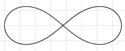
Figure 1: The figure-eight

.

First we will consider genus one cases, including genus zero, studied by Euler and Bernoulli. Using the isometric deformation $Z(\delta t)=Z(0)+\delta t\partial_{t}Z(0)$ ($\partial_{t}Z(0)=(v^{(r)}+{\mathrm{i}}v^{(i)})\partial_{s}Z$), after the Goldstein-Petrich method [17], we consider the minimal problem for the EB energy [31]. For the deformation, we require $\displaystyle{\frac{{\mathcal{E}}_{\rm{EB}}[Z(\delta t)]-{\mathcal{E}}_{\rm{EB}}[Z(0)]}{v^{(r)}\delta t}=0}$ modulo $\delta t$. This yields the static MKdV equation, $a\kappa+\frac{1}{2}\kappa^{3}+\partial_{s}^{2}\kappa=0,$ associated with the elliptic curve $(\partial_{s}\kappa)^{2}+\frac{1}{4}\kappa^{4}+a\kappa^{2}+b=0,$ where $a$ and $b$ are integral constants [31]. Let us consider the elliptic curve $X_{1}$ ($\hat{y}=2y$ in (8) $g=1$) in the Weierstrass standard form [50],

$$\hat{y}^{2}=4(x-b_{1})(x-b_{2})(x-b_{3}),$$ (12)

where $b_{1}=-\frac{1}{6}a$, $b_{2}=\frac{1}{12}a+\frac{1}{4}\sqrt{b}$, and $b_{3}=\frac{1}{12}a-\frac{1}{4}\sqrt{b}$ satisfying $a^{2}-b=16$. We identify the coordinate $u=(u_{1})$ of the complex plane ${\mathbb{C}}$ with $u_{1}$ and $u=v_{1}(x,y)$ for $(x,y)\in X_{1}$.

Lemma 3.2

Let ${\mathrm{e}}^{2{\mathrm{i}}\varphi}:=(x-b_{1})/\gamma$ for $e_{c-1}:=b_{c}-b_{1}$ and $\gamma=\sqrt{e_{1}e_{2}}$. The holomorphic one-form (9) is

$$du=\frac{2k\,d\varphi}{\sqrt{1-k^{2}\sin^{2}\varphi}},$$ (13)

where $\gamma=1$, $(\sqrt{e_{2}}-\sqrt{e_{1}})^{2}=(a-4)/2$ and the modulus $\displaystyle{k:=\frac{2{\mathrm{i}}\root 4 \of{e_{2}e_{1}}}{\sqrt{e_{2}}-\sqrt{e_{1}}}=\sqrt{\frac{8}{4-a}}}$.

In the cases of genera zero and one, it is easy to impose the conditions CI-III, i.e., $\partial_{u{\mathrm{r}}}\psi_{\mathrm{i}}=0$, $du_{{\mathrm{i}}}=0$ by $|x-b_{1}|$ $=\gamma$, and therefore we are concerned with $\phi=\psi_{\mathrm{r}}=2\varphi_{\mathrm{r}}$, which obeys (2) and (11).

The solutions are expressed by the Jacobi elliptic functions, cf., e.g. [22, 38, 49]; therefore, they can instead be written in terms of the Weierstrass elliptic functions [31]; the latter can be generalized to higher genus and they are briefly reviewed in the introduction to Section 3 [28, 31]. In this paper, in order to evaluate these solutions numerically, we show that Euler’s figure eight is directly expressed by means of Euler’s method, though current mathematical software easily reproduces Euler’s original results; our computation in Figure 1 shows a simple numerical method suffices.

1. $g=0$ case: We consider the limit of $k\to 0$ with $2kd\varphi=ds$. By identifying $du$ with $ds$, we have the circle as the minimal path of the EB energy.

2. $g=1$ case: We let $du=ds$, $k=2.398107502$ for $a=2.608918126$. We numerically evaluate the figure-eight curve of in Figure 1, as illustrated in Euler’s book [15]: here we plot $Z(s)=(X+{\mathrm{i}}Y)(s)$ as a function of $s$. We used Euler’s approximation method, $\varphi(s+\delta)\approx\varphi(s)+\frac{\partial\varphi}{\partial s}\delta$ and $Z(s+\delta)=Z(s)+{\mathrm{e}}^{2{\mathrm{i}}\varphi}\delta$ for a small number $\delta$. In the computations, $\varphi$ moves back and forth in the interval $[\varphi_{s},\varphi_{e}]$ where $\varphi_{s}=\sin^{-1}(k^{-2})\in[0,\pi/2)$ and $\varphi_{e}=\pi-\varphi_{s}$.

3.2 Genus Two

In this subsection, we investigate the conditions CI-III for hyperelliptic curves $X_{2}$ of genus $g=2$. It turns out that in order to obtain the solution of (2) based on Theorem 3.1, we need higher-genus hyperelliptic curves ($g>2$). However, we show that even data in $S^{2}X_{2}$ give trajectories for generalization of elastica cf. Figure 3 and Figure 7.

We choose coordinates $u={}^{t}(u_{1},u_{2})$ in ${\mathbb{C}}^{2}$; $u_{i}=u_{i}^{(1)}+u_{i}^{(2)}$ where $u_{i}^{(j)}=v_{i}((x_{j},y_{j}))$.

We let $a=5$ in Theorem 3.1, $b_{5}=-\gamma=-1$, and $e_{c}:=b_{c}-b_{5}$ $(c=1,2,3,4)$.

We restrict the moduli (or parameter) space of the curve $X_{2}$ by the following:

Conditions: $\sqrt{e_{2a-1}}=\alpha_{a}+{\mathrm{i}}\beta_{a}$, $\sqrt{e_{2a}}=\alpha_{a}-{\mathrm{i}}\beta_{a}$ where $\alpha_{a},\beta_{a}\in{\mathbb{R}}$, $a,b=1,2$, satisfying $\alpha_{a}^{2}+\beta_{a}^{2}=\gamma$.

Under this assumption, we have the natural extension of genus-one elastica; indeed, direct computation shows the following:

Lemma 3.3

Let $\gamma{\mathrm{e}}^{2{\mathrm{i}}\varphi}:=(x-b_{5})$, (8) $g=2$ is

$$y^{2}=16\frac{\gamma^{5}{\mathrm{e}}^{6{\mathrm{i}}\varphi}}{k_{1}^{2}k_{2}^{2}}(1-k_{1}^{2}\sin^{2}\varphi)(1-k_{2}^{2}\sin^{2}\varphi)$$ (14)

where $\displaystyle{k_{a}=\frac{2{\mathrm{i}}\sqrt[4]{e_{2a-1}e_{2a}}}{\sqrt{e_{2a-1}}-\sqrt{e_{2a}}}=\frac{\sqrt{\gamma}}{\beta_{a}}}$, $(a=1,2)$.

We consider a point $((x_{1},y_{1}),(x_{2},y_{2}))$ in $S^{2}X_{2}$ under the condition CI, $|x_{c}-b_{5}|=\gamma$. We define the variable $\varphi_{a}$ by $x_{c}=\gamma{\mathrm{e}}^{{\mathrm{i}}\varphi_{c}}({\mathrm{e}}^{{\mathrm{i}}\varphi_{c}}+(b_{5}/\gamma){\mathrm{e}}^{-{\mathrm{i}}\varphi_{c}})$ $(c=1,2)$. Noting $dx_{c}=2{\mathrm{i}}\gamma{\mathrm{e}}^{2{\mathrm{i}}\varphi_{c}}d\varphi_{c}$ and $x_{c}dx_{c}=-4\gamma{\mathrm{e}}^{3{\mathrm{i}}\varphi_{c}}\sin\varphi_{c}\ d\varphi_{c}$, we have the holomorphic one forms $(du_{1}^{(c)},du_{2}^{(c)})$ $(c=1,2)$,

$$\left(\frac{(\sin\varphi_{c}+{\mathrm{i}}\cos\varphi_{c})\ d\varphi_{c}}{2\gamma K(\varphi_{c})},-\frac{\sin\varphi_{c}\ d\varphi_{c}}{K(\varphi_{c})}\right),$$ (15)

where $\displaystyle{K(\varphi):=\frac{\sqrt{\gamma(1-k_{1}^{2}\sin^{2}\varphi)(1-k_{1}^{2}\sin^{2}\varphi)}}{k_{1}k_{2}}}$.

Lemma 3.4

Let $K_{c}:=K(\varphi_{c})$. The following holds:

1. $\displaystyle{\left(\begin{array}[]{c}du_{1}\\ du_{2}\end{array}\right)=\left(\begin{array}[]{cc}\frac{{\mathrm{i}}\exp(-{\mathrm{i}}\varphi_{1})}{2\gamma K_{1}}&\frac{{\mathrm{i}}\exp(-{\mathrm{i}}\varphi_{2})}{2\gamma K_{2}}\\ \frac{-\sin(\varphi_{1})}{K_{1}}&\frac{-\sin(\varphi_{2})}{K_{2}}\end{array}\right)\left(\begin{array}[]{c}d\varphi_{1}\\ d\varphi_{2}\end{array}\right)}$,

2. $\displaystyle{\left(\begin{array}[]{c}\partial_{u_{1}}\\ \partial_{u_{2}}\end{array}\right)=\frac{2\gamma K_{1}K_{2}}{{\mathrm{i}}\sin(\varphi_{2}-\varphi_{1})}\left(\begin{array}[]{cc}-\frac{\sin(\varphi_{2})}{K_{2}}&\frac{\sin(\varphi_{1})}{K_{1}}\\ -\frac{{\mathrm{i}}\exp(-{\mathrm{i}}\varphi_{2})}{2\gamma K_{2}}&\frac{{\mathrm{i}}\exp(-{\mathrm{i}}\varphi_{1})}{2\gamma K_{1}}\end{array}\right)\left(\begin{array}[]{c}\partial_{\varphi_{1}}\\ \partial_{\varphi_{2}}\end{array}\right)}$.

Due to Lemma 3.4 and the expression $\varphi_{c}=\varphi_{c{\mathrm{r}}}+{\mathrm{i}}\varphi_{c{\mathrm{i}}}$, we have

$$\frac{\partial\varphi_{1{\mathrm{i}}}}{\partial u_{2\,{\mathrm{r}}}}=\frac{K_{1}\sin\varphi_{2{\mathrm{r}}}}{\sin(\varphi_{1{\mathrm{r}}}-\varphi_{2{\mathrm{r}}})},\quad\frac{\partial\varphi_{2{\mathrm{i}}}}{\partial u_{2\,{\mathrm{r}}}}=\frac{K_{2}\sin\varphi_{1{\mathrm{r}}}}{\sin(\varphi_{2{\mathrm{r}}}-\varphi_{1{\mathrm{r}}})}$$ (16)

and $\psi=2(\varphi_{1}+\varphi_{2})$ satisfies (10) and (11).

Figure 2: The orbit $C$ of $\partial_{u_{2}\,{\mathrm{r}}}\psi_{\mathrm{i}}=$constant: $\varphi_{1{\mathrm{r}}}$ depends on $\varphi_{2{\mathrm{r}}}$ for Figure3 (c). The arrow shows the direction of $d\eta$.

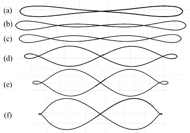
Figure 3: Generalized elastica of genus two, where $(k_{1},k_{2})$ are as follows: (a):(1.60,2.20), (b):(1.90,2.15), (c) $(2.08,2.32)$, (d): $(3.08,3.32)$, (e): $(3.80.4.20)$, (f):(4.00,10.00).

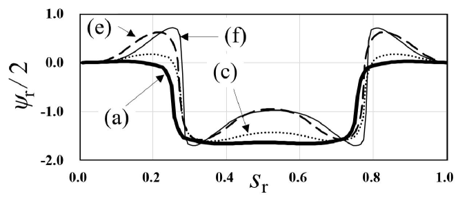
Figure 4: $\psi_{\mathrm{r}}/2$ of Figure 3 (a), (c), (e), and (f).

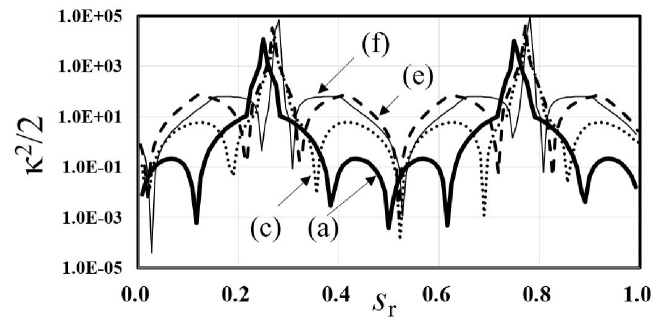
Figure 5: $\kappa^{2}/2$ of Figure 3 (a), (c), (e), and (f).

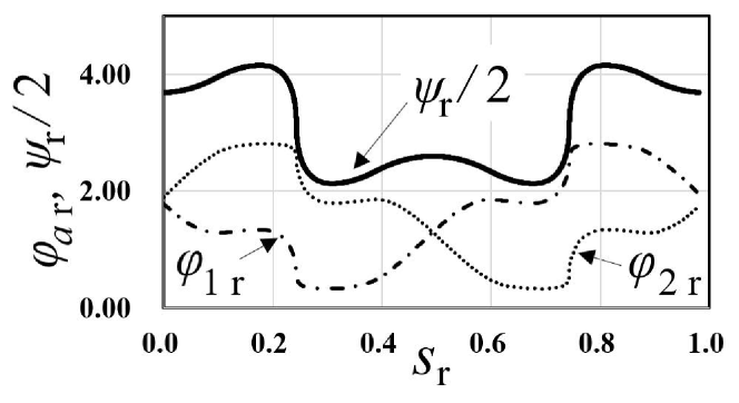
Figure 6: The decomposition of $\psi_{\mathrm{r}}/2$ to $\varphi_{1{\mathrm{r}}}$ and $\varphi_{2{\mathrm{r}}}$ of Figure 3 (d).

Let us investigate the conditions CII and CIII. Assume $A(u)=\varepsilon\gamma$; then, ${\left(\begin{array}[]{c}\partial_{t}\\ \partial_{s}\end{array}\right)=\left(\begin{array}[]{cc}-4&-4\varepsilon\gamma\\ 0&1\end{array}\right)\left(\begin{array}[]{c}\partial_{u_{1}}\\ \partial_{u_{2}}\end{array}\right)}$ in (11) shows the correspondence between the Abelian parameters $(u_{1},u_{2})$ and $(t,s)$ in the MKdV equation (2) via ${\left(\begin{array}[]{c}dt\\ ds\end{array}\right)=\left(\begin{array}[]{cc}-1/4&0\\ \varepsilon\gamma&1\end{array}\right)\left(\begin{array}[]{c}du_{1}\\ du_{2}\end{array}\right)}$. Using this expression, $dt=dt_{\mathrm{r}}+{\mathrm{i}}dt_{\mathrm{i}}$ and $ds=ds_{\mathrm{r}}+{\mathrm{i}}ds_{\mathrm{i}}$, we have the following lemma:

Lemma 3.5

$\displaystyle{\left(\begin{array}[]{c}dt_{\mathrm{r}}\\ dt_{\mathrm{i}}\\ ds_{\mathrm{r}}\\ ds_{\mathrm{i}}\end{array}\right)=M\left(\begin{array}[]{cc}d\varphi_{1{\mathrm{r}}}\\ d\varphi_{1{\mathrm{i}}}\\ d\varphi_{2{\mathrm{r}}}\\ d\varphi_{2{\mathrm{i}}}\end{array}\right)}$ where

$$M:=\left(\begin{array}[]{cccc}-\frac{\sin\varphi_{1}}{8\gamma K_{1}}&\frac{\cos\varphi_{1}}{8\gamma K_{1}}&-\frac{\sin\varphi_{2}}{8\gamma K_{2}}&\frac{\cos\varphi_{2}}{8\gamma K_{2}}\\ -\frac{\cos\varphi_{1}}{8\gamma K_{1}}&-\frac{\sin\varphi_{1}}{8\gamma K_{1}}&-\frac{\cos\varphi_{2}}{8\gamma K_{2}}&-\frac{\sin\varphi_{2}}{8\gamma K_{2}}\\ \frac{(2+\varepsilon)\sin\varphi_{1}}{2K_{1}}&-\frac{\varepsilon\cos\varphi_{1}}{2K_{1}}&\frac{(2+\varepsilon)\sin\varphi_{2}}{2K_{2}}&-\frac{\varepsilon\cos\varphi_{2}}{2K_{2}}\\ \frac{\varepsilon\cos\varphi_{1}}{2K_{1}}&\frac{(2+\varepsilon)\sin\varphi_{1}}{2K_{1}}&\frac{\varepsilon\cos\varphi_{2}}{2K_{2}}&\frac{(2+\varepsilon)\sin\varphi_{2}}{2K_{2}}\\ \end{array}\right).$$ (17)

Due to condition CI, $d\varphi_{1{\mathrm{i}}}=d\varphi_{2{\mathrm{i}}}=0$, and thus we have $dt_{\mathrm{r}}\propto ds_{\mathrm{r}}$.

We consider the condition CIII, i.e., an orbit $C$ of constant $\partial_{u_{2}{\mathrm{r}}}\psi_{\mathrm{i}}$ in the $\varphi_{1{\mathrm{r}}}$-$\varphi_{2{\mathrm{r}}}$ plane by requiring

$$d\left(\frac{\partial\psi_{{\mathrm{i}}}}{\partial u_{2\,{\mathrm{r}}}}\right)=\frac{\partial(\partial_{u_{2}{\mathrm{r}}}\psi_{{\mathrm{i}}})}{\partial\varphi_{1{\mathrm{r}}}}d\varphi_{1{\mathrm{r}}}+\frac{\partial(\partial_{u_{2}{\mathrm{r}}}\psi_{{\mathrm{i}}})}{\partial\varphi_{2{\mathrm{r}}}}d\varphi_{2{\mathrm{r}}}=0,$$ (18)

using (16). By parameterizing $C$ by $\eta\in{\mathbb{R}}$, we have the curve equation,

$$d\varphi_{1{\mathrm{r}}}=\frac{\partial(\partial_{u_{2}{\mathrm{r}}}\psi_{{\mathrm{i}}})}{\partial\varphi_{2{\mathrm{r}}}}d\eta,\quad d\varphi_{2{\mathrm{r}}}=-\frac{\partial(\partial_{u_{2}{\mathrm{r}}}\psi_{{\mathrm{i}}})}{\partial\varphi_{1{\mathrm{r}}}}d\eta,$$ (19)

On $C$, $\psi$, $s$ and $t$ are functions of $\eta\in{\mathbb{R}}$. This implies that $ds_{{\mathrm{i}}}\neq 0$ in general.

Due to the number of conditions CI, CII, and CIII and the degrees of freedom of the real parameters $u_{1}$ and $u_{2}$, the consistency between CII and CIII is crucial.

We obtain $C$ by numerically solving (19) as in Figure 2 using Euler’s method. In the computations, $\varphi_{a}$ moves back and forth in the interval $[\varphi_{s},\varphi_{e}]$ where $\varphi_{s}=\sin^{-1}(k_{1}^{-2})\in[0,\pi/2)$ and $\varphi_{e}=\pi-\varphi_{s}$. Since $\varphi_{s}$ and $\varphi_{e}$ are branch points in $X_{2}$ (the interval $[\varphi_{s},\varphi_{e}]$ corresponds to one of the homology basis of $X_{2}$), the sign of $K_{a}$ changes at the turns.

Due to multiplication by $M$ in (17), $ds_{{\mathrm{r}}}$ vanishes on the line $L:\varphi_{1{\mathrm{r}}}=\pi-\varphi_{2{\mathrm{r}}}$ in the $\varphi_{1{\mathrm{r}}}$-$\varphi_{2{\mathrm{r}}}$ plane. For our $g=2$ case, there exist crossing points between the line $L$ and the orbit $C$ (Figure 2), and at the points $ds_{{\mathrm{r}}}$ vanishes whereas $ds_{{\mathrm{i}}}$ (or $du_{2{\mathrm{i}}}$) does not. Thus $\displaystyle{\frac{d\psi_{{\mathrm{r}}}}{ds_{{\mathrm{r}}}}=\frac{\partial\psi_{{\mathrm{r}}}}{\partial s_{{\mathrm{r}}}}-\frac{\partial\psi_{{\mathrm{r}}}}{\partial s_{{\mathrm{i}}}}\frac{ds_{\mathrm{i}}}{ds_{{\mathrm{r}}}}}$ diverges at the points. Since $g=2$, the crossing occurs for any parameters $k_{c}$ $(c=1,2)$, the divergence shows that the conditions CII and CIII are contradictory, and thus we cannot find the solution of (2) based on Theorem 3.1 in genus two. To satisfy the conditions, we need higher-genus hyperelliptic curves $X_{g}$ $(g>2)$.

However, the pole behavior of $d\psi_{{\mathrm{r}}}/ds_{{\mathrm{r}}}$ is of type $1/\sqrt{s_{\mathrm{r}}-s_{{\mathrm{r}}0}}$ at $s_{\mathrm{r}}=s_{{\mathrm{r}}0}$ up to a constant factor. Therefore $\psi_{\mathrm{r}}$ can be defined as a hyperelliptic (2-branch) function of $s_{{\mathrm{r}}}$ using the data in Theorem 3.1 along $C$. Since for finite $\delta\eta$, we obtain $\delta\varphi_{c{\mathrm{r}}}$ $(c=1,2)$ by (19), we compute $\delta s_{\mathrm{r}}$ by using $M$ in (17), and approximate $Z(s_{\mathrm{r}}+\delta s_{\mathrm{r}})\approx Z(s_{\mathrm{r}})+{\mathrm{e}}^{2(\varphi_{1{\mathrm{r}}}+\varphi_{2{\mathrm{r}}}){\mathrm{i}}}\delta s_{\mathrm{r}}$ using Euler’s method for appropriate initial data $\varphi_{a}(s=0,t=0)$ so that $Z$ is periodic in $s_{\mathrm{r}}$; since $Z$ is in general not periodic, we determine appropriate initial states by the shooting method with the bisection process.

Finally, we numerically obtain the shapes of a generalization of the elastica of genus two in Figure 3. Though they are not solutions of (2), they identically satisfy (10) and are a natural extension of Euler’s results. We also numerically compute and display their $\psi_{\mathrm{r}}$ in Figure 4 and the energy density $\kappa^{2}/2$ in Figure 5.

3.3 Comparison of elastica’s periodic orbits and DNA

We offer a few remarks that provide evidence, for the shapes that we obtained, to actually exhibit the geometry of supecoiled DNA.

Coleman and Swigon classify the equilibrium configurations of a knot-free loop [13, Figure 1]; Arnold gives a complete list using topological indices [1, Figure 11]. Figure 3 (b)-(f) corresponds to (d) in the Coleman-Swigon list [13] and $(0,0,-3)$ in Arnold’s list [1] whereas Figure 3 (a) and Figure 1 correspond to (b) in [13] and $(0,0,-1)$ in [1] respectively. The last entries $-3$ and $-1$ in Arnold’s symbol correspond to the number of self-contact points with minus sign, $-i(Z)$ in this case. It is noted that the shapes in Figure 3 have the same zero winding number as the figure-eight, $w^{(1)}=0$.

Since the shapes in Figure 3 satisfy (10) for genus two (though they are not solutions of (2)), we can bring them as evidence because they reproduce some properties of the AFM or EMS images of the supercoiled DNA [5, 8, 20, 23, 48]; Figure 24-8 in [48] displays the five electron micrographs of DNA (mini ColE1 plasmid dimer, 5kb) by Laurien Polder [20, p.36, Figure 1-19], which shows the supercoiling from fully relaxed to tightly coiled. The two of them which have four and six self-contact points, i.e., $(0,0,-4)$ and $(0,0,-6)$ in Anold’s symbol, with ‘weak elastic forces’, resemble Figure 3 (b) and (c), though the number of self-contact points differ. As in the AFM images of mini plasmid, 688bp [23, Figures 1, 2], we find distorted circle and figure-eight, i.e., $(0,0,0)$ and $(0,0,-1)$ in Anold’s symbol, both correspond to the solutions in elliptic functions in subsection 3.1 and Figure 3 (a). On the other hand, the large plasmid in [8, Figure 3], [5, Figures 2 and 3], [23, Figures 1 and 2], and figure [20, 48] have more complicated shapes with larger self-contact numbers. Some of them are the loops with Anold’s symbol $(0,0,-\ell)$, $(\ell\geq 5)$ with ‘weak elastic forces’, and Figure 3 (b)-(f) reproduce such properties though they pertain to the $\ell=3$ case

The $\psi_{\mathrm{r}}$ in Figure 4 exhibits 1) periodicity and 2) mixing of so-called kink (anti-kink) type mode and breather type mode [2]; due to the kink type mode, the energy density (or elastic force) is localized (cf. Figure 5) and has a singularity; the local extrema correspond to the two points of maximal curvature of the loops in Figure 3.

The mixing of both modes turns out to be a higher-genus phenomenon, not present in genus one. The $\psi_{\mathrm{r}}$ in Figure 4 consists of $\varphi_{1{\mathrm{r}}}$ and $\varphi_{2{\mathrm{r}}}$ and the addition of both form the mixing; we show it for the case (c) in Figure 6. Since genus 2 gives two parameters $\varphi_{a{\mathrm{r}}}$, there are various (non unique) types of mixing and we have the family of shapes in Figure 3, which reproduce the shapes of DNA.

3.4 Considerations on the energy of the orbits

To reproduce the shapes of the supercoiled DNA mathematically, several models are proposed (cf. Introduction) based on Euler’s elastica. However, in these approaches even three dimensional effects such as twist and other perturbative effects cannot exhibit the mixing. Indeed, we consider the minima of the energy as in subsection 3.1: by fixing the boundary conditions (the winding number and the number of the self-contacts), the minimum should be uniquely determined. Since the image of $v$ in (9) for $g=1$ is one dimensional, the elliptic functions represent only one of the kink solution or breather-type solution, and as in subsection 3.1, the shape is rather simple.

In [13, 44], the writhing modes were demonstrated using a real thick rubber rod in [44, Figure 8] and numerical elastic rods with finite thickness [13, Figures 7 and 8] which must preserve the self-contacts. However if one takes the limit of the rod’s thickness to zero to model Euler’s elastica, the loops must collapse. This contradicts the observation in [5, 23, 48]; In general, the supercoiled DNAs have shapes whose self-intersection does not change even taking the limit of their thickness to zero. Therefore, shapes with minimal energy and topological constraints do not recover the shapes of supercoiled DNAs in general, and we have to consider additional effects such as the thermal effect. This results in the MKdV equation (2) and MKdV hierarchy (7). The associated Riemann surfaces of higher genus demonstrate the structure of DNA, which requires excited states.

Our results in Figure 3 provide such shapes with the number of self-contact numbers $i(Z)>1$ with ‘weak elastic forces’ like observed DNA. We computed them in genus two. We expect that the closed orbits of generalized elastica with higher genus have a larger number of contact points, and faithfully reproduce the observed DNA shapes.

As mentioned in Section 2, on a physical model of DNA, the EB energy is a component of the total energy (5). Since the singularity of the energy density is of type $ds_{{\mathrm{r}}}/(s_{{\mathrm{r}}}-s_{{\mathrm{r}}0})$, it can be removed by introducing a cut-off parameter. Thus by fixing the cut-off parameter, we may propose the shapes in Figure 3 as a physical model: for example, we may regard Figure 3 as a transition of shapes from (a) to (f) (and further to figure-eight) depending on the variation of the temperature and the difference of their energy; like ${\mathcal{Z}}^{(0,1)}[\beta]$ in the $n=1$ case in Section 2, the number of self-contact points have effects on the transition depending on $\alpha_{1}$ in (5) though $\alpha_{2}$, the coefficient of the winding number in (5), does not have any effect on it.

If we extend our model to three dimensions [11, 12, 16, 27], our results in Figure 3 naturally bring in the writhing numbers, which are part of the geometry of DNA. When we consider the statistical mechanics of elastica in three-dimensional space, their configurations are given by the torsion $\tau(s)$ and the curvature $\kappa(s)$ [27]. The complex curvature $\displaystyle{\kappa_{c}=\kappa\exp\left(\int^{s}\tau(s)ds\right)}$ naturally appears. If we employ the EB energy using $\kappa^{2}=\overline{\kappa_{c}}\kappa_{c}$, the NLS and CmKdV hierarchies provide the isometric and the iso-energy deformations instead of the MKdV hierarchy for the elastica in a plane. Several elastic models in three dimensional space are proposed. Since the topological invariant for the strip is given by the linking number $\mathrm{Lk}$ which consists of the writhing number $\mathrm{wr}$ and the twisting number $\mathrm{tw}$, i.e., $\mathrm{Lk}=\mathrm{wr}+\mathrm{tw}$, these topological properties directly relate to the shapes; for example, if we consider them as global effects, or define the total energy $E_{\mathrm{total}}=E_{\mathrm{EB}}+\alpha_{3}\mathrm{wr}+\alpha_{4}\mathrm{tw}$ for coupling constants $\alpha_{3}$ and $\alpha_{4}$, they influence the distributions of shapes as mentioned in the toy model ${\mathcal{Z}}^{(0,1)}[\beta]$ in Section 2. The models depend on how we treat these effects of the writhing and twisting locally by certain elastic forces (by coupling with the torsion $\tau(s)$ and the curvature $\kappa(s)$) and/or globally. When we employ the simplest energy $E_{\mathrm{EB}}$ even in the three dimensional model for simplicity, the CmKdV and the NLS equations, which are complex valued [14, 34, 41], appear instead of the MKdV equation [12, 16, 27]. Due to the complex-valued setting, we expect that the difficulty in solving the equations identified in this paper might be avoided even for $g=2$ and the writhing-like shapes in Figure 3 might be realized as real writhing in three-dimensional space, by exactly solving the PDE.

Lastly, we note that by similar computations, lifting the condition CIII (19) but adding CII $ds_{{\mathrm{i}}}=0$, the gauged MKdV equation (11) yields more intricate shapes (cf. Figure 7).

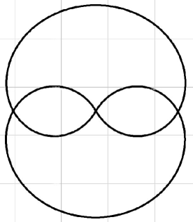
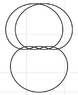
(a)                                            (b)

Figure 7: Solutions of (11) of genus two, where $(k_{1},k_{2})$ are as follows: (a): $(4.52,10.0)$, (b): $(7.47,10.0)$.

4 Conclusion

We proposed an algebro-geometric method to plot loops, as trajectories of generalized of elastica. We concluded that we cannot find the solution of the MKdV equation (2) based on our algebraic data in Theorem 3.1 for $X_{2}$ $g=2$ and that higher-genus curves ($g\geq 3$) are required to find the solution of (2).

Even though they are not solutions of the MKdV equation over ${\mathbb{R}}$, since they identically satisfy the MKdV equation over ${\mathbb{C}}$ (10) and are a natural generalization of Euler’s elastica, we demonstrated the typical shapes in Figures 3 and 7 in terms of the hyperelliptic functions using the data in Theorem 3.1. They partially recover some geometrical properties of the AFM or EMS images of the supercoiled DNA, cf., e.g., [8, 48]. In order to recover the shapes of the supercoiled DNA, our algebro-geometrical approach is crucial.

By extension to higher genus curves and three dimensional space as in [12, 16, 27], it is expected that the energy and topological properties of the supercoiled DNA would be clarified.

S.M. acknowledges support by JSPS KAKENHI Grant Number JP21K03289. The authors thank the anonymous referees for crucial comments and one of them for her/his suggestion to refer to [38].

References

- [1] V. I. Arnold, Topological Invariants of Plane Curves and Caustics, (University Lecture Series), AMS. 1994.
- [2] M. J. Ablowitz and H. Segur, Solitons and the inverse scattering transform, SIAM 1981.
- [3] H.F. Baker, Abelian functions, Cambridge Univ. Press, Cambridge, 1995 Reprint of the 1897 original.
- [4] R. Baxter, Exactly Solved Models in Statistical Mechanics, Academic Pr, 1982.
- [5] P. Bettotti, V. Visone, L. Lunelli, G. Perugino, M. Ciaramella, and A, Valenti, Structure and Properties of DNA Molecules Over The Full Range of Biologically Relevant Supercoiling States, Sci. Rep., 8 (2018) 6163.
- [6] M.Born, Stabilität der elastischen Linie in Ebene und Raum, Preisschrift und Dissertation, Göttingen, Dieterichsche Universitäts-Buchdruckerei Göttingen, 1906.
- [7] C. Bouchiat and M. Mézard, Elastic rod model of a supercoiled DNA molecule, Eur. Phys. J. E 2 (2000) 377–402.
- [8] T. Brouns, H. De Keersmaecker, S. F. Konrad, N. Kodera, T. Ando, J. Lipfert, S. De Feyter, and W. Vanderlinden, Free Energy Landscape and Dynamics of Supercoiled DNA by High-Speed Atomic Force Microscopy, ACS Nano. 12 (2018) 11907–11916.
- [9] V.M. Buchstaber, V.Z. Enolskiĭ and D.V. Leĭkin, Kleinian functions, hyperelliptic Jacobians and applications, Rev. Math. Math. Phys., 10 (1997) 1–103.
- [10] C. R. Calladine, H. Drew, B. Luisi and A. Travers, Understanding DNA, 3rd ed., Academic Press, 2004.
- [11] G. S. Chirikjian, The Stochastic Elastica and Excluded-Volume Perturbations of DNA Conformational Ensembles, Int J Non Linear Mech. 43, (2008) 1108–1120.
- [12] G. S. Chirikjian, Framed curves and knotted DNA, Biochem. Soc. Trans. 41, (2013) 635–638.
- [13] B. D. Coleman and D. Swigon, Theory of Supercoiled Elastic Rings with Self-Contact and Its Application to DNA Plasmids, J. Elasticity 60 (2000), 173-221, 2000.
- [14] J. C. Eilbeck and V. Z. Enolskii and N. A. Kostov, Quasiperiodic and periodic solutions for vector nonlinear Schrödinger equations, J. Math. Phys., 41 (2000) 8236–8248.
- [15] L. Euler, Methodus Inveniendi Lineas Curvas Maximi Minimive Proprietate Gaudentes, 1744, Leonhardi Euleri Opera Omnia Ser. I vol. 14.
- [16] R. E. Goldstein and S. A. Langer, Nonlinear Dynamics of Stiff Polymers, Phys. Rev. Lett., 75 (1995) 1094–1097.
- [17] R.E. Goldstein and D.M. Petrich, The Korteweg-de Vries hierarchy as dynamics of closed curves in the plane, Phys. Rev. Lett., 67 (1991) 3203–3206.
- [18] S. Goyal, N.C. Perkins, and C.L. Lee, Nonlinear dynamics and loop formation in Kirchhoff rods with implications to the mechanics of DNA and cables, J. Comp. Phys., 209 (2005) 371–389.
- [19] C. Itzykson and J.-M. Drouffe, Statistical Field Theory: Vol.1, 2, , Cambridge Univ. Press. 1991.
- [20] A. Kornberg and T. A. Baker, DNA Replication, W. H. Freeman & Co, 1992.
- [21] E. A. Kümmerle, and E. Pomplun, A computer-generated supercoiled model of the pUC19 plasmid, Eur Biophys J., 34 (2005) 13-8.
- [22] A. E. H. Love, A Treatise on the Mathematical Theory of Elasticity, Cambridge Univ. Press 1927.
- [23] Y. L. Lyubchenko and L. S. Shlyakhtenko, Visualization of supercoiled DNA with atomic force microscopy in situ, Proc. Natl. Acad. Sci. USA, 94 (1997) 496-501.
- [24] S. Lim, Y. Kim and D. Swigon, Dynamics of an electrostatically charged elastic rod in fluid, Proc. R. Soc. A 467 (2011) 569-590.
- [25] F. Maggioni, F. A. Potra, and M. Bertocchi, Optimal Kinematics of a Looped Filament, J. Optim. Theory Appl. (2013) 159 489-506.
- [26] S. Matsutani, , Statistical mechanics of elastica on a plane: origin of the MKdV hierarchy, J. Phys. A: Math. & Gen., 31 (1998) 2705–2725.
- [27] S. Matsutani, , Statistical mechanics of non-stretching elastica in three dimensional space, J. Geom. Phys., 29 (1999) 243–259.
- [28] S. Matsutani, Hyperelliptic loop solitons with genus : investigation of a quantized elastica, J. Geom. Phys., 43 (2002) 146-162.
- [29] S. Matsutani, Reality conditions of loop solitons genus g, Elec. J. Diff. Eqns. 2007 (2007) 1–12.
- [30] S. Matsutani, Relations in a quantized elastica, J. Phys. A: Math. Theor., 41 (2008) 075201(12pp).
- [31] S. Matsutani, Euler’s Elastica and Beyond, J. Geom. Symm. Phys 17 (2010).
- [32] S. Matsutani and Y. Ônishi On the Moduli of a Quantized Elastica in and KdV Flows: Study of Hyperelliptic Curves as an Extension of Euler’s Perspective of Elastica I, Rev. Math. Phys., 15 (2003) 559–628.
- [33] S. Matsutani and E. Previato, From Euler’s elastica to the mKdV hierarchy, through the Faber polynomials, J. Math. Phys., 57 (2016) 081519.
- [34] E. Previato, Hyperelliptic quasi-periodic and soliton solutions of the nonlinear Schrödinger equation, Duke Math. J., 52 (1985) 329–377.
- [35] E. Previato, Geometry of the modified KdV equation, in LNP 424: Geometric and quantum aspects of integrable systems Ed. by G. F. Helminck, Springer 1993, 43–65.
- [36] A. L. B. Pyne, A. Noy, , K.H.S. Main, et al., Base-pair resolution analysis of the effect of supercoiling on DNA flexibility and major groove recognitionby triplex-forming oligonucleotides, Nature Comm. 12 (2021) 1053.
- [37] P. Ramond, Field Theory: A Modern Primer (Frontiers in Physics, , Basic Books. 1990.
- [38] Y. L. Sachkov Closed Euler elasticae, Proc. Steklov Inst. Math., 278 (2012) 218-232.
- [39] E. L. Starostin, Closed loops of a thin elastic rod and its symmetric shapes with self-contacts, PAMM, Proc. Appl. Math. Mech.1 (2002) 21–25.
- [40] Y. Shi and J. E. Hearst, The Kirchhoff elastic rod, the nonlinear Schrödinger equation, and DNA supercoiling, J. Chem. Phys. 101 (1994) 5186-5200.
- [41] H. J. Shin, Vortex filament motion under the localized induction approximation in terms of Weierstrass elliptic functions, Phys. Rev. E, 65 (2002) 036317.
- [42] D. Swigon, B. D. Coleman, and I. Tobias, The Elastic Rod Model for DNA and Its Application to the Tertiary Structure of DNA Minicircles in Mononucleosomes, Biophysical J., 74 (1998) 2515–2530.
- [43] C. J. Thompson, Mathematical Statistical Mechanics, Princeton Univ. Press, 1972.
- [44] A. A. Travers, G. Muskhelishvili, and J. M. T. Thompson, DNA information: from digital code to analogue structure, Phil. Trans. R. Soc. A, 370 (2012) 2960–2986.
- [45] C. Truesdell The influence of elasticity on analysis: the classic heritage Bull. Amer. Math. Soc., 9 (1983) 293–310.
- [46] H. Tsuru, Equilibrium shapes and vibrations of thin elastic rod, J. Phys. Soc.Japan, 56 (1987) 2309–2324.
- [47] H. Tsuru and M. Wadati, Elastic Model of Highly Supercoiled DNA, Biopolymers, 25 (1986) 2083–2096.
- [48] D Voet and J. G. Voet, Fundamentals of Biochemistry: Life at the Molecular Level, 4th ed., Wiley 2015.
- [49] M. Wadati and H. Tsuru, Elastic Model of looped DNA, Physica D, 21 (1986) 213–226.
- [50] E.T. Whittaker and G.N. Watson, A Course of Modern Analysis,, Cambridge Univ. Press 1927.