Mathematical optimization models for long-term maintenance scheduling of wind power systems

Abstract

During the life of a wind farm, various types of costs arise. A large share of the operational cost for a wind farm is due to maintenance of the wind turbine equipment; these costs are especially pronounced for offshore wind farms and they provide business opportunities in the wind energy industry. An effective scheduling of the maintenance activities may reduce the costs related to maintenance.

We combine mathematical modelling of preventive maintenance scheduling with corrective maintenance strategies. We further consider different types of contracts between the wind farm owner and a maintenance or insurance company, and during different phases of the turbines’ lives and the contract periods. Our combined preventive and corrective maintenance models are then applied to relevant combinations of the phases of the turbines’ lives and the contract types.

Our case studies show that even with the same initial criteria, the optimal maintenance schedules differ between different phases of time as well as between contract types. One case study reveals a $40~{}\%$ cost reduction and a significantly higher production availability—$1.8~{}\%$ points—achieved by our optimization model as compared to a pure corrective maintenance strategy. Another study shows that the number of planned preventive maintenance occasions for a wind farm decreases with an increasing level of an insurance contract regarding reimbursement of costs for broken components.

1 Introduction

Global warming is an important issue nowadays from many points of view, since it will lead to serious global consequences for both humans and nature. Global warming has been attributed to increased greenhouse gas emission concentrations in the atmosphere through the burning of fossil fuels. To reduce these concentrations, wind power can be used to replace energy from fossil fuels. A wind farm can generate energy all day and night, as long as there is wind. Wind power is an abundant renewable energy provider, which produces almost no greenhouse gases during operation. According to [5], wind power is one of the technologies that produce zero greenhouse gas emissions. Currently, the U.S. wind industry employs more than $100000$ workers, and according to [6], the wind has the potential to support more than $600000$ jobs in manufacturing, installation, maintenance, and supporting services by the year $2050$ in the U.S.

During the life of a wind farm, various kinds of costs arise. In the beginning, there are costs for, e.g., renting the premises, building permits, and the construction of the wind turbines. During the years of operation, there are maintenance costs, costs for grid transport of electricity, personnel costs, etc. When the wind turbine is outworn, costs arise for tearing it down. A large share of the operational cost for a wind farm is due to maintenance of the wind turbine equipment; these costs are especially pronounced for offshore wind farms and they provide business opportunities in the wind energy industry. An effective way to reduce the costs related to maintenance is to employ an improved methodology for scheduling the maintenance activities. In this article, we investigate the planning of two types of maintenance activities, i.e., corrective maintenance and preventive maintenance.

Corrective maintenance (CM) means to maintain a component after a failure has occurred. Then there will be a production loss and the failure may also affect the remaining lives of other components. The cost of CM is, therefore, a combination of component costs, damage costs (for other components), and costs due to lost production (during the time from the failure until replacement).

Preventive maintenance (PM) means to maintain a component before it fails; it is a pre-scheduled maintenance activity. The component cost is then typically lower than the corresponding CM cost and there are no damage costs of other components. Further, the downtime of the equipment is typically shorter than under CM, due to PM being pre-scheduled; hence, the loss of revenue from the production is smaller.

The wind turbine maintenance industry involves four types of stakeholders: manufacturers, wind farm owners, maintenance companies, and insurance companies. The maintenance is performed by either the manufacturer, the farm owner, a contracted maintenance company, or a temporarily hired maintenance company; the interrelations of the companies involved are regulated by contracts. We consider the following four contract types, all of which are common within wind energy production and maintenance.

1. Full service production-based maintenance contract (between the wind farm owner and the manufacturer). Maintenance is performed by the manufacturer, who covers the costs for replacement related to all component failures. The contract also guarantees a minimum ’level of measured average availability’ of the wind farm, defined as ’available production divided by the sum of available and unavailable production’. The manufacturer plans for PM; if a component suddenly fails the manufacturer performs CM of the broken component. A variant of this type of contract includes a time-based warranty, which guarantees a minimum ’level of technical availability of the wind farm’, defined as ’the total share of each given time interval during which the wind farm is available for operation’. Under this contract—since the manufacturer pays for all maintenance costs—we optimize the PM scheduling on behalf of the manufacturer.

2. Basic insurance contract (between the party who pays for the maintenance and the insurance company). Maintenance is performed either by a maintenance company or by the wind farm owner’s maintenance team. When a component fails due to a ’sudden failure’ there is a need for CM of that component. The insurance company will reimburse the farm owner for the cost of the component with a discount, while the work/labour costs are paid by the wind farm owner. In practice, the stakeholders negotiate in order to classify a failure as a sudden failure or not; in our modelling this negotiation is represented by a probability that ’the failure is classified as being sudden’. Since a sudden failure entails unwanted costs for both stakeholders, they both benefit from performing PM, where the extent depends on the value of the probability. Under this contract, the wind farm owner and the insurance company share the components’ costs during a CM activity. Hence, the PM scheduling is optimized on behalf of the wind farm owner.

3. No insurance contract. Maintenance is performed either by a maintenance company or by the wind farm owner’s maintenance team. The wind farm owner covers all its costs for maintenance. The wind farm owner plans for PM; if a component suddenly fails the owner asks a maintenance company or its own maintenance team to perform CM. Under this contract—since the wind farm owner pays for all maintenance costs—the maintenance scheduling is optimized on behalf of the wind farm owner.

4. Maintenance contract with a maintenance company (between the wind farm owner and the maintenance company). Four main types of agreements exist:

   • Call-off agreement. The simplest variant; the wind farm owner contacts the service provider in the event of an error. The wind farm owner pays for the working hours required for the maintenance and for the components as the costs occur.

   • Basic agreement. The planned service is included in an annual fee; CM is paid by the wind farm owner when it occurs. This agreement is available both with and without remote monitoring.

   • Full service ”light”. The planned service, corrective maintenance, and spare parts, monitoring, as well as reporting, are included in an annual fee. The main components (blade/rotor, main bearing, gearbox, generator, nacelle, tower, and foundation) are excluded. Inverters and SCADA systems are either included or excluded. This agreement can be with or without an availability guarantee (time- or production/energy-based).

   • Full service. The planned service, CM (including spare parts and main components), monitoring, and reporting are included in the agreement. Blade wear–and–tear are included in certain agreements. Foundations are not included. This agreement comes with an availability guarantee, which is time- or production-based.

   We assume that related to the main component, this contract can be characterized as either of the contract types [C-I], [C-II], or [C-III]. For the call-off agreement, the basic agreement and full service ”light” agreement the optimal scheduling strategy will be similar to that of [C-III]. For the full service agreement, the optimal scheduling strategy will be similar to that of [C-I].

According to discussions with a group of wind farm owners within the Swedish Wind Power Technology Centre (SWPTC) [1], two different set-ups are commonly experienced. One set-up is to have a [C-I] contract with the manufacturer from the beginning till the end of life of the wind farm. The other set-up is to have a [C-I] contract with the manufacturer during the initial years of a wind farm’s operating period, after which the wind farm owner either extends this contract (type [C-I]), or acquires a contract with a maintenance company (type [C-IV]), or acquires a basic insurance contract (type [C-II]), or has no insurance contract (type [C-III]); during the life of the wind farm, the owner may switch between the four contract types.

Regardless of the type of contract that applies during each given time period, the wind turbines need to be continuously maintained throughout their lives. From a maintenance planning perspective, the interrelations of the end of the planning period considered, the end of the current contract period, and the end of the life of the wind farm are used to define the following three phases of time.

1. The normal phase: After the end of the planning period there is still a long period of time left for the contract period as well as for the life of the wind farm. The maintenance company thus cares about component failures also after the end of the planning period. We address this responsibility by imposing penalties that grow with the ages of the respective components that are present in the turbine at the end of the planning period.

2. The phase close to the end of a full service production-based maintenance contract (presuming a contract of type [C-I]): The end of the planning period coincides with the end of the contract period. The maintenance company needs to ensure that the wind farm is functioning at the contracted level of availability until the end of the planning period; the maintenance company is not responsible for any component failures after the end of the planning period.

3. The phase close to the end of life of the wind farm (presuming a contract of type [C-II] or [C-III]): The end of the planning period coincides with the end of life of the wind farm. Hence, it may be non-beneficial to maintain any components that fail (very) close to the end of the planning period.

We will study four principal cases that are relevant for the planning of PM and which are characterized by the above definitions of contracts and phases.

First, we consider the case when the wind farm and the maintenance company has a contract of type [C-I] and the maintenance company is responsible for the maintenance. We propose in Section 4.1 a flexible mathematical optimisation model for finding optimal maintenance plans in the phase [P-ii]. The model finds a PM schedule over the planning period such that the costs of performing maintenance are minimized. The availability constraints encountered in phase [P-ii] are modelled as the expected average (over the planning period) number of available turbines.

Section 4.2 considers a wind farm owner with a contract of either type [C-I] or type [C-III]. In phase [P-i] our model finds a PM schedule over the planning period such that the costs of performing maintenance are minimized. The maintenance costs are supplemented by penalty costs based on the ages of the component individuals in the turbine(s) at the end of the planning period.

In Section 4.3 we consider a wind farm owner without any insurance contract, i.e., with a contract of type [C-III], and in the phase [P-iii]. The model finds a PM schedule over the planning period such that the costs of performing maintenance are minimized; it also finds an optimal time, after which CM should not be performed.

Section 4.4 considers a wind farm owner having a basic insurance contract, i.e., a contract of type [C-II]. Our model then seeks to minimize the maintenance costs, while accounting for a certain probability that the insurance company will pay for new components at CM. The relation between the price of an insurance contract and the cost of an optimal maintenance plan—for the case of having no insurance contract—is also modelled.

The four principal cases are modelled using a framework of mathematical modelling, which is described in the introductory sections of the paper. In Section 2 we review relevant literature on (industrial) maintenance planning and contracting between the wind farm owner/operator and the maintenance provider. Section 3 describes our basic mathematical model for finding feasible PM schedules for a farm of wind turbines, the modelling of expected costs for pure CM strategies, costs for PM scheduling, and combinations of these; this results in so-called interval costs for component replacements; the modelling of costs is based on Weibull distributed failure times of the components. In Section 4, the four principal cases are described, followed by the reporting in Section 5 of results from a set of case studies. Finally, in Section 6 we draw conclusions from the results of the case studies and propose further research topics.

2 Literature review

Before the 20th century, maintenance cost was considered to be a kind of inevitable cost, and most maintenance actions performed considered corrective maintenance. In 1929, the idea of preventive maintenance by daily, weekly, and general inspections was introduced in [16]. Since then, maintenance methodology has grown quite fast. There is a broad body of literature devoted to various strategies of maintenance scheduling. In this article, we look at maintenance scheduling methods from different perspectives.

In the paper by Yeh and Chen [19], a mathematical model to derive an optimal periodical PM policy for a leased facility is developed. Within a lease period, any failures of the facility are rectified by minimal repairs and a penalty may occur to the lessor when the time required to perform a minimal repair exceeds a reasonable time limit. Further on, Lee and Cha [11] considered periodic PM policies for a deteriorating repairable system, and the effect of each PM action is classified into one of the three categories ’failure rate reduction’, ’decrease of deterioration speed’, and ’age reduction’.

While periodical PM policies consider equidistant PM occasions, Gustavsson et al. [9] and Moghaddam and Usher [13] study PM scheduling over a long time period. The model PMSPIC in [9] was devised to schedule PM of the components of a system over a finite and discretized time horizon, given a common set-up cost and component costs dependent on the lengths of the maintenance intervals; the model can be used for PM scheduling as well as be dynamically used in a setting allowing for rescheduling. In [13] optimization models are developed that determine optimal PM schedules for repairable and maintainable systems. It is demonstrated that higher set-up costs make simultaneous PM activities beneficial. The suggested models are, however, nonlinear, meaning that they are computationally hard to solve.

Jafari et al. [10] propose a joint optimization of the maintenance policy and the inspection interval for a multi-unit series system. The authors develop a model and algorithm which are used to determine a maintenance policy that minimizes the maintenance cost for a multi-component system; in the system studied, one unit is subject to condition monitoring, while for the other unit, only age information is available and which has a general distribution. Tian et al. [18] develop a method that uses the condition monitoring data to effectively predict the remaining life of a component in a multi-component system.

The papers [7, 12, 14, 15] are devoted to optimization issues related to different maintenance contracts. Park and Pham [14] deal with the optimal maintenance policy under different warranty policies, considering both the warranty period and the post-warranty period. For the warranty period, the authors suggest a warranty cost model using a repair–replacement warranty policy considering repair as well as failure times. Qiu et al. [15] consider optimization of the maintenance costs under performance-based contracts. The paper investigates an optimal maintenance policy for inspected systems that are subject to both soft and hard failures. According to de Almeida [7], the main parameters of maintenance contracts are downtime and maintenance costs. Lisnianski et al. [12] consider an aging system, in which the maintenance is performed by an external maintenance team. Different kinds of contracts between the two parties are considered, with special attention paid to downtime costs (i.e., the loss of revenue due to production stops). The authors suggest a model based on a piece-wise constant approximation of the increasing failure rate function.

3 Mathematical modelling of maintenance planning for a farm of wind turbines

We consider the maintenance planning for a wind farm comprising $m$ wind turbines (indexed by $i\in\mathcal{I}:=\{1,\ldots,m\}$) each of which has $n$ (identical) component types (indexed by $j\in\mathcal{J}:=\{1,\ldots,n\}$).

During the usage of a wind turbine its components will degrade and—if not repaired or replaced—one or more components will eventually fail; then, CM will have to be performed in the form of component replacement. We will model the failure rates such that the survival function of a component of type $j\in\{1,\ldots,n\}$ comes from a Weibull distribution with scale parameter $\alpha_{j}>0$ and shape parameter $\beta_{j}>0$.

Our models are defined over a time period—denoted by the continuous time interval $[0,T]$—such that a (new) wind turbine starts production at time $0$, while its life ends at time $T$. Part of our modelling employs a finite set of discrete time steps, indexed by $\{1,\ldots,T\}$, where time step $t\in\{1,\ldots,T\}$ represents the time interval $[t-1,t]\subset[0,T]$. A maintenance contract (abbreviated as c) period covers a time interval $[{s_{\text{c}}},{e_{\text{c}}}]\subseteq[0,T]$, such that ${e_{\text{c}}}\geq{s_{\text{c}}}+1$, i.e., a time period covering the time steps indexed by $\{{s_{\text{c}}}+1,\ldots,{e_{\text{c}}}\}\subseteq\{1,\ldots,T\}$. Analogously, a maintenance planning (abbreviated as p) period covers a time interval $[{s_{\text{p}}},{e_{\text{p}}}]\subseteq[0,T]$, such that ${e_{\text{p}}}\geq{s_{\text{p}}}+1$, i.e., a time period covering the time steps indexed by $\{{s_{\text{p}}}+1,\ldots,{e_{\text{p}}}\}\subseteq\{1,\ldots,T\}$. Figure 1 illustrates the time steps and the corresponding continuous time intervals.

Figure 1: Illustration of the notation for the continuous and normalized time (above the time line) and the corresponding time steps (below the time line) used in the models.

3.1 A basic mathematical model defining a feasible PM schedule

The mathematical model (1), below, is an adaption to our settings of the model of the preventive maintenance scheduling problem with so-called interval costs, as developed in [9]. It considers the planning period $({s_{\text{p}}},{e_{\text{p}}}]$, indexed by $\{{s_{\text{p}}}+1,\ldots,{e_{\text{p}}}\}$, during which PM actions can be scheduled.

The variables of the model are defined as follows. For each wind turbine $i\in\mathcal{I}$ and component type $j\in\mathcal{J}$, and any two indices $u\in\{{s_{\text{p}}},\ldots,{e_{\text{p}}}\}$ and $t\in\{u+1,\ldots,{e_{\text{p}}}+1\}$, $x^{ij}_{ut}=1$ if PM is planned at time steps $u$ and $t$, but no PM is planned in-between these; otherwise $x^{ij}_{ut}=0$. Whenever $x^{ij}_{ut}=1$, we say that a PM interval for component $(i,j)$ starts at time step $u$ and ends at time step $t$. For each wind turbine $i\in\mathcal{I}$ and any two indices $u\in\{{s_{\text{p}}},\ldots,{e_{\text{p}}}-1\}$ and $t\in\{{s_{\text{p}}}+1,\ldots,{e_{\text{p}}}\}$, the variable $y^{i}_{ut}=1$ if PM is planned at time steps $u$ and $t$, but no PM is planned in-between these for at least one of its component types at time $t$; otherwise $y^{i}_{ut}=0$; see (1c). Further, for any two indices $u\in\{{s_{\text{p}}},\ldots,{e_{\text{p}}}-1\}$ and $t\in\{{s_{\text{p}}}+1,\ldots,{e_{\text{p}}}\}$, the variable $z_{ut}=1$ if PM is planned at time steps $u$ and $t$, but no PM is planned in-between these for any of the components in the farm at time $t$; otherwise $z_{ut}=0$; see (1d).

$$\sum_{t={s_{\text{p}}}+1}^{{e_{\text{p}}}+1}x^{ij}_{{s_{\text{p}}}t} =1,\ i\in\mathcal{I},\ j\in\mathcal{J},$$ (1a)

$$\sum_{u={s_{\text{p}}}}^{t-1}x^{ij}_{ut} =\sum_{v=t+1}^{{e_{\text{p}}}+1}x^{ij}_{tv}, i\in\mathcal{I},\ j\in\mathcal{J},\ t={s_{\text{p}}}+1,\ldots,{e_{\text{p}}},\$$ (1b)

$$y_{ut}^{i} \geq x^{ij}_{ut}, i\in\mathcal{I},\ j\in\mathcal{J},\ u={s_{\text{p}}},\ldots,t-1,$$ (1c)

$$t={s_{\text{p}}}+1,\ldots{e_{\text{p}}},\$$

$$z_{ut} \geq y_{ut}^{i}, i\in\mathcal{I},\ u={s_{\text{p}}},\ldots,t-1,$$ (1d)

$$t={s_{\text{p}}}+1,\ldots{e_{\text{p}}},$$

$$x^{ij}_{ut} \in\{0,1\},\ i\in\mathcal{I},\ j\in\mathcal{J},\ u={s_{\text{p}}},\ldots,t-1,$$ (1e)

$$t={s_{\text{p}}}+1,\ldots{e_{\text{p}}}+1,\$$

$$y^{i}_{ut},z_{ut} \in\{0,1\},\ i\in\mathcal{I},\ u={s_{\text{p}}},\ldots,t-1,$$ (1f)

$$t={s_{\text{p}}}+1,\ldots{e_{\text{p}}}.\$$

Due to the constraints (1a), for each component $(i,j)$ either the first PM is scheduled in one of the time steps $\{{s_{\text{p}}}+1,\ldots,{e_{\text{p}}}\}$, or no PM is scheduled (i.e., $x^{ij}_{{s_{\text{p}}},{e_{\text{p}}}+1}=1$). The constraints (1b) make sure that, for each component $(i,j)$, the end of any PM interval is the start of the next PM interval.

Consider a point which is feasible subject to the constraints (1), and which is such that for all $(i,j)$ and all $u\in\{{s_{\text{p}}},\ldots,t-1\}$ and $t\in\{{s_{\text{p}}}+1,\ldots,{e_{\text{p}}}+1\}$, $x^{ij}_{ut}=0$, except that $x^{ij}_{{s_{\text{p}}},{e_{\text{p}}}+1}=1$, and such that for all $i$ and all $t\in\{{s_{\text{p}}}+1,\ldots,{e_{\text{p}}}\}$, $y_{ut}^{i}=z_{ut}=0$. This point corresponds to planning no PM activities during the planning period $[{s_{\text{p}}},{e_{\text{p}}}]$ and is referred to as a pure CM plan; the corresponding situation will be modelled further in Section 3.2.

3.2 Modelling of costs for CM strategies and PM scheduling

We next define the parameters used for the types of costs incurred by different maintenance activities, and describe the calculation of the expected maintenance costs of a CM strategy, and how these interact with a planned PM schedule. We also introduce a number of parameters to be used as building blocks of the models to be defined in the following sections.

3.2.1 Cost and time parameters

For each component type $j\in\mathcal{J}$, we define the following time-independent parameters representing cost for maintenance activities: $g_{j}^{\tiny\text{\tiny CM}}$ denotes the cost of a new component of type $j$ at a CM action; $b_{j}^{\tiny\text{\tiny CM}}$ denotes the cost of a new component (i.e., $g_{j}^{\tiny\text{\tiny CM}}$) plus the logistics costs (i.e., transport, set-up, and work costs for the crane, and manpower costs for the replacement) of a CM action; $c_{j}^{\text{\tiny PM}}$ denotes the cost of a new component minus the value (i.e., the expected sales revenue) of the replaced component, plus the cost (e.g., work cost for the crane and manpower cost for the replacement) of the PM action.

The costs and revenues that are common to all component types, but dependent on the time step $t\in\{1,\ldots,T\}$, are defined as follows: $d_{t}$ denotes the cost attributed to a specific wind turbine, incurred by any maintenance activity at time $t$; $f_{t}$ denotes the costs shared by the wind turbines of a farm (e.g., crane transport and set-up costs) incurred by any maintenance activity at time $t$; $r_{t}\geq 0$ denotes the revenue (in terms of the monetary value of the energy produced) created by a fully functioning turbine during time step $t\in\{1,\ldots,T\}$, i.e., during the continuous time period $[t-1,t]\subset[0,T]$.

The amount of time required for performing a CM (of component $j\in\mathcal{J}$) and a PM action are denoted by $\gamma_{j}^{\tiny\text{\tiny CM}}>0$ and $\gamma^{\text{\tiny PM}}>0$, respectively.

3.2.2 Revenue function and revenue loss

The total revenue created by a functioning wind turbine during the time period $[v+\lambda,T]$, where $v\in\{0,\ldots,T-1\}$ and $\lambda\in[0,1]$, is expressed by the revenue function $R:[0,T+\bar{\gamma}]\mapsto\mathbb{R}_{+}$, where $\bar{\gamma}:=\max\{\gamma^{\text{\tiny PM}};\max_{j\in\mathcal{J}}\{\gamma_{j}^{\tiny\text{\tiny CM}}\}\}$, and which is defined by

$$R(u) :=0, u\in[T,T+\bar{\gamma}];$$ (2a)

$$R(v+\lambda) :=(1-\lambda)r_{v+1}+R(v+1), \lambda\in[0,1],\,v\in\{T-1,\ldots,0\}.$$ (2b)

From the definition (2) follows that the revenue function $R$ is piece-wise affine, continuous, and non-increasing on the time interval $[0,T+\bar{\gamma}]$.

The revenue loss caused by a production stop during the time interval between the two (continuous) time points $u\in[0,T]$ and $u+w\in[u,T+\bar{\gamma}]$ is then given by

$$R^{\text{\tiny loss}}(u,w) :=R(u)-R(u+w).$$ (3)

Utilizing the definitions in Section 3.2.1 we conclude that the revenue loss caused by a CM action of component $j$ at the (continuous) time $t\in[0,T]$ equals $R^{\text{\tiny loss}}(t,\gamma_{j}^{\tiny\text{\tiny CM}})$, while the revenue loss caused by a PM action of any component at time step $t\in\{1,\ldots,T\}$ equals $R^{\text{\tiny loss}}(t,\gamma^{\text{\tiny PM}})$.

3.2.3 Failure times and induced CM costs

For each wind turbine $i\in\mathcal{I}$ and component type $j\in\mathcal{J}$ a number of component individuals will consecutively be put to work in the turbine. Let $\tau_{u}^{ij}\in[0,u]$ denote the age of the current component individual at (the end of) time step $u\in\{1,\ldots,T\}$. Further, for $k=1,2,\ldots$, let $L_{k}^{ij}>0$ denote the life of the $k$’th consecutive component individual in use in the turbine, where $k=1$ corresponds to the current (i.e., at time step $u$) individual. The $k$’th failure time for a component of type $j$ in turbine $i$, after the (current) time step $u$ (i.e., after the continuous time $u$), is then expressed as

$$U_{uk}^{ij} :=u-\tau_{u}^{ij}+\sum_{\ell=1}^{k}L_{\ell}^{ij}, k=1,2,\ldots.$$

We also define $U_{u0}^{ij}:=u-\tau_{u}^{ij}$ and assume independent, identically Weibull distributed individual component lives $L_{k}^{ij}\sim\text{W}(\alpha_{j},\beta_{j})$, $k=1,2,\ldots$ . Specifically, the life distribution of the current individual (i.e., $k=1$) is conditioned on its age $\tau_{u}^{ij}$ at time step $u$. Hence, it holds that

$$P(L_{1}^{ij}\geq v\,|\,L_{1}^{ij}\geq\tau^{ij}_{u}) =\left\{\begin{array}[]{ll}1,&v\in[0,\tau^{ij}_{u}],\\ \exp\bigg{[}\Big{(}\frac{\tau^{ij}_{u}}{\alpha_{j}}\Big{)}^{\beta_{j}}-\Big{(}\frac{v}{\alpha_{j}}\Big{)}^{\beta_{j}}\bigg{]},&v\geq\tau^{ij}_{u},\end{array}\right.$$

and

$$P(L_{k}^{ij}\geq v) =\exp\bigg{[}{-\Big{(}\frac{v}{\alpha_{j}}\Big{)}^{\beta_{j}}}\bigg{]},\qquad v\geq 0,\quad k=2,3,\ldots.$$

Any failure of a component type $j\in\mathcal{J}$ in a turbine $i\in\mathcal{I}$ at time $t\in[0,T]$ induces a cost of a CM action which amounts to

$$b_{j}^{\tiny\text{\tiny CM}}+R^{\text{\tiny loss}}(t,\gamma_{j}^{\tiny\text{\tiny CM}}).$$ (4)

3.2.4 Expected cost of a pure CM strategy

We denote by ${F}_{ut}^{{\tiny\text{\tiny CM}}\,ij}$ the expected cost associated with the maintenance of a component type $j\in\mathcal{J}$ in a turbine $i\in\mathcal{I}$ during a time interval $[u,t]$ under a pure CM strategy, which is such that no PM is scheduled during the time interval considered. It is defined as the expectation of the sum of component costs and revenue losses, as

$${F}_{ut}^{{\tiny\text{\tiny CM}}\,ij}:=\mathbb{E}\left[\sum_{k=1}^{\infty}1_{\{U_{uk}^{ij}\leq t\}}\Big{(}b_{j}^{\tiny\text{\tiny CM}}+R^{\text{\tiny loss}}(U_{uk}^{ij},\gamma_{j}^{\tiny\text{\tiny CM}})\Big{)}\right].$$ (5)

Algorithm 1 describes how to compute ${F}_{ut}^{{\tiny\text{\tiny CM}}\,ij}$. The expected sum of component costs and revenue losses associated with CM actions of a wind farm under a pure CM strategy during the time interval $[{s_{\text{p}}},{e_{\text{p}}}]$ is then defined as ${F}_{{s_{\text{p}}}{e_{\text{p}}}}^{{\tiny\text{\tiny CM}}\,}:=\sum_{i\in\mathcal{I}}\sum_{j\in\mathcal{J}}{F}_{{s_{\text{p}}}{e_{\text{p}}}}^{{\tiny\text{\tiny CM}}\,ij}$.

Result: ${F}_{ut}^{{\tiny\text{\tiny CM}}\,ij}$

Input: $i\in\mathcal{I}$, $j\in\mathcal{J}$, $u\in\{1,\ldots,T-1\}$, $t\in\{u+1,\ldots,T\}$, $\tau_{u}^{ij}\in[0,u]$, $M\gg 1$, $b_{j}^{\tiny\text{\tiny CM}}$, $R:\ [0,T]\mapsto\mathbb{R}_{+}$

for $\ell=1,\ldots,M$ do

       $k:=0$ ; $U_{u0}^{ij}:=u-\tau_{u}^{ij}$ ; $a_{\ell}:=0$ ;

       while $U_{uk}^{ij}\leq t\,$  do

             $k:=k+1$ ;

             Generate $L_{k}^{ij}$ based on the survival function ;

             $U_{uk}^{ij}:=U_{u,k-1}^{ij}+L_{k}^{ij}$ ;

             $a_{\ell}:=a_{\ell}+b_{j}^{\tiny\text{\tiny CM}}+R^{\text{\tiny loss}}(U_{uk}^{ij},\gamma_{j}^{\tiny\text{\tiny CM}})$ ;

            

       end while

      

end for

${F}_{ut}^{{\tiny\text{\tiny CM}}\,ij}:=M^{-1}\sum_{\ell=1}^{M}a_{\ell}$ ;

Algorithm 1 Numerical computation of expected CM costs ${F}_{ut}^{{\tiny\text{\tiny CM}}\,ij}$, defined in (5), for a component type $j$ in a turbine $i$ during the time interval $[u,t]$

3.2.5 Failure times and PM cost savings

In the case when PM is scheduled but components fail before their planned PM, a need for CM actions arises.

Consider a schedule for the PM of a wind farm over a specific time interval, and let $u$ and $t>u$ denote two time steps within that interval at each of which there is a planned PM action, but no PM is planned in-between these two time steps, for a component type $j\in\mathcal{J}$ in a turbine $i\in\mathcal{I}$.

If a component type $j\in\mathcal{J}$ fails at a time $\sigma\in[u,t]$, then a CM action must be performed at time $\sigma$ (inducing a CM cost according to (4)). A rescheduling of the planned PM due to this failure then leads to a possible reduction of the costs $c_{j}^{\text{\tiny PM}}$ associated with the planned PM action for the component type $j$ and turbine $i$ at time step $t$. We denote this reduction by the PM cost savings function $\phi_{ut}^{\text{\tiny PM}}:[u,t]\mapsto[0,1]$. For $\sigma=u$, meaning that the component individual would fail immediately after it is put to use in the turbine and that a CM action is indeed performed at time step $u$, the state of this component type is retained and the current PM schedule remains optimal; hence, it holds that $\phi_{ut}^{\text{\tiny PM}}(u)=0$. For $\sigma=t$, the rescheduling would amount to removing the scheduled PM action for component type $j$ at time step $t$, and replacing it by a CM action; then, all the associated PM costs are saved and it holds that $\phi_{ut}^{\text{\tiny PM}}(t)=1$.

It is reasonable to assume that the PM cost savings function is non-decreasing with the failure time $\sigma\in[u,t]$, and we will further assume that the function $\phi_{ut}^{\text{\tiny PM}}$ is linear. This results in the expression

$$\phi_{ut}^{\text{\tiny PM}}(\sigma):=\frac{\sigma-u}{t-u},\qquad\sigma\in[u,t].$$

Considering the case of $n\geq 1$ failures at times $\sigma_{k}$, $k=1,\ldots,n$, such that $u\leq\sigma_{1}\leq\sigma_{2}\leq\ldots\leq\sigma_{n}\leq t$, the PM cost savings function is generalised as

$$\phi_{ut}^{\text{\tiny PM}}(\sigma_{1},\ldots,\sigma_{n}) :=\frac{\sigma_{1}-u}{t-u}+\sum_{k=2}^{n}\frac{\sigma_{k}-\sigma_{k-1}}{t-u}=\frac{\sigma_{n}-u}{t-u}.$$ (6)

From (6) follows that only the time $\sigma_{n}$ of the last failure within the time interval $[u,t]$, for component type $j\in\mathcal{J}$ in a turbine $i\in\mathcal{I}$, will affect the PM cost savings function.

Recalling that $U_{uk}^{ij}$ denotes the time of the $k$’th failure for a component type $j$ in a turbine $i$, after the time step $u$, we conclude that the time of the last failure of the component can be expressed as

$$\max\left\{\,u\,;\,\max_{k\geq 0}\left\{\,U_{uk}^{ij}\,\big{|}\,U_{uk}^{ij}\leq t\,\right\}\,\right\}.$$ (7a)

We then regard the effect of component failures on the savings of the costs $$d_{t}+R^{\text{\tiny loss}}(t,\gamma^{\text{\tiny PM}}) f_{t} \sigma_{n} [u,t] i\in\mathcal{I}$$ and , on the wind turbine and wind farm levels, respectively. Reasoning analogously as above, the time of the last failure in the time interval of any component in a turbine is expressed as

$$\max\left\{u;\max_{j\in\mathcal{J}}\left\{\max_{k\geq 0}\left\{U_{uk}^{ij}\,\big{|}\,U_{uk}^{ij}\leq t\right\}\right\}\right\},$$ (7b)

while the time $$\sigma_{n} [u,t]$$ of the last failure in the time interval of any component in any turbine in the wind farm, is expressed as

$$\max\left\{u;\max_{i\in\mathcal{I},j\in\mathcal{J}}\left\{\max_{k\geq 0}\left\{U_{uk}^{ij}\,\big{|}\,U_{uk}^{ij}\leq t\right\}\right\}\right\}.$$ (7c)

3.2.6 Failure-free time intervals

For each wind turbine $i\in\mathcal{I}$, each component type $j\in\mathcal{J}$, each time step $u\in\{1,\ldots,T-1\}$ of the previous PM of the component, and each $t\in\{u+1,\ldots,T\}$, we can now express the expected proportion of the failure-free, right-most subset of the time interval $[u,t]$ as

$$p_{ut}^{ij}:=\frac{1}{t-u}\cdot\left(t-\mathbb{E}\left[\max\left\{u;\max_{k\geq 0}\left\{U_{uk}^{ij}\,\big{|}\,U_{uk}^{ij}\leq t\right\}\right\}\right]\right).$$ (8a)

These proportions can be numerically computed according to Algorithm 2.

For each wind turbine $i\in\mathcal{I}$, each time step $u\in\{1,\ldots,T-1\}$ of the previous PM occasion for the turbine, and each $t\in\{u+1,\ldots,T\}$, the corresponding failure-free proportion of the time interval $[u,t]$ equals

$$p_{ut}^{i}:=\frac{1}{t-u}\cdot\left(t-\mathbb{E}\left[\max\left\{u;\max_{j\in\mathcal{J}}\left\{\max_{k\geq 0}\left\{U_{uk}^{ij}\,\big{|}\,U_{uk}^{ij}\leq t\right\}\right\}\right\}\right]\right).$$ (8b)

On the wind farm level, for each time step $u\in\{1,\ldots,T-1\}$ of the previous PM occasion for the farm, and each $t\in\{u+1,\ldots,T\}$, the corresponding failure-free proportion of the time interval $[u,t]$ equals

$$p_{ut}:=\frac{1}{t-u}\cdot\left(t-\mathbb{E}\left[\max\left\{u;\max_{i\in\mathcal{I},j\in\mathcal{J}}\left\{\max_{k\geq 0}\left\{U_{uk}^{ij}\,\big{|}\,U_{uk}^{ij}\leq t\right\}\right\}\right\}\right]\right).$$ (8c)

Result: $p_{ut}^{ij}$

Input: $i\!\in\!\mathcal{I}$, $j\!\in\!\mathcal{J}$, $u\!\in\!\{1,\ldots,T\!-\!1\}$, $t\!\in\!\{u\!+\!1,\ldots,T\}$, $\tau_{u}^{ij}\!\in\![0,u]$, $M\!\gg\!1$

for $\ell=1,\ldots,M$ do

       $k:=0$ ; $U_{u0}^{ij}:=u-\tau_{u}^{ij}$ ;

       repeat

             $k:=k+1$ ;

             Generate $L_{k}^{ij}$ based on the survival function ;

             $U_{uk}^{ij}:=U_{u,k-1}^{ij}+L_{k}^{ij}$ ;

             $a_{\ell}:=U_{u,k-1}^{ij}$

      until $U_{uk}^{ij}>t$;

      if $k=1$ then

            $a_{\ell}:=u$

       end if

      

end for

$p_{ut}^{ij}:=(t-u)^{-1}\big{(}t-M^{-1}\sum_{\ell=1}^{M}a_{\ell}\big{)}$

Algorithm 2 Numerical computation of $p_{ut}^{ij}$, defined in (8a), for a component type $j$ in a turbine $i$ during the time interval $[u,t]$

3.2.7 Interval costs

We define the interval cost of a PM action at time step $t$ on a component type $j$ of turbine $i$, when the previous maintenance of the same component type was performed at time step $u\leq t-1$, as the sum of the cost of the scheduled PM action at time $t$, the revenue loss caused by the PM action at time $t$, and the expected CM costs for the component type $j$ of turbine $i$ over the time interval $[u,t]$. For the case when a CM action is not accompanied by a rescheduling of the PM schedule (see Section 3.2.4), the interval cost over the time interval $[u,t]$ is thus defined as

$${F}_{ut}^{{\tiny\text{\tiny CM}}\,ij}+c_{j}^{\text{\tiny PM}},$$

where ${F}_{ut}^{{\tiny\text{\tiny CM}}\,ij}$ is defined in (5). For the case when a CM action is accompanied by a rescheduling of the PM schedule, part of the cost $c_{j}^{\text{\tiny PM}}$ can be saved, and the interval cost over the time interval $[u,t]$ is defined as

$${F}_{ut}^{{\tiny\text{\tiny CM}}\,ij}+c_{j}^{\text{\tiny PM}}p_{ut}^{ij},$$

where $p_{ut}^{ij}$ is defined in (8a).

4 Modelling of PM scheduling under different phases and contracts

The four combinations of contracts and phases that are relevant for the planning of PM of wind farms are described in the following subsections.

4.1 Full service production-based contract

Here, we consider the phase close to the end of a full service production-based maintenance contract, i.e., phase [P-ii] and contract type [C-I]. The planning period is then defined as the time interval $[{s_{\text{p}}},{e_{\text{c}}}]$.

Hence, for $t={s_{\text{p}}}+1,\ldots,{e_{\text{c}}}+1$, $u={s_{\text{p}}},\ldots,t-1$, $i\in\mathcal{I}$, and $j\in\mathcal{J}$, we define the sum of expected component costs and revenue losses as

$$C_{ut}^{ij}:= {F}_{ut}^{{\tiny\text{\tiny CM}}\,ij}+c_{j}^{\text{\tiny PM}}p_{ut}^{ij}, t\in\{{s_{\text{p}}}\!+\!1,\ldots,{e_{\text{c}}}\}$$ , (9a)

$$C_{ut}^{ij}:= {F}_{u,{e_{\text{c}}}}^{{\tiny\text{\tiny CM}}\,ij}, t={e_{\text{c}}}\!+\!1$$ , (9b)

where ${F}_{ut}^{{\tiny\text{\tiny CM}}\,ij}$ and $p_{ut}^{ij}$, are defined in (5) and (8a), respectively. Letting $p_{ut}^{i}$ and $p_{ut}$ be defined by (8b) and (8c), respectively, for any pair $(s,e)$ of indices such that $s\geq 0$ and $e\in\{s+1,\ldots,T\}$, we define the function $G^{\text{\tiny PM}}_{se}$ of PM costs over the time interval $[s,e]$, on the turbine and farm levels as

$$G^{\text{\tiny PM}}_{se}(\mathbf{y},\mathbf{z}):=\sum_{u=s}^{e-1}\sum_{t=u+1}^{e}\left(\Big{(}d_{t}+R^{\text{\tiny loss}}(t,\gamma^{\text{\tiny PM}})\Big{)}\sum_{i\in\mathcal{I}}p_{ut}^{i}y^{i}_{ut}+f_{t}p_{ut}z_{ut}\right).$$ (10)

Letting $C^{ij}_{ut}$ be defined by (9), an optimal PM plan is then obtained by minimizing the sum of expected costs for CM and the costs for the PM occasions during the time period $[{s_{\text{p}}},{e_{\text{c}}}]$, according to

$$\mathop{\text{minimise }}_{\mathbf{x},\mathbf{y},\mathbf{z}} \sum_{u={s_{\text{p}}}}^{{e_{\text{c}}}}\sum_{t=u+1}^{{e_{\text{c}}}+1}\sum_{i\in\mathcal{I}}\sum_{j\in\mathcal{J}}C^{ij}_{ut}x^{ij}_{ut}+G^{\text{\tiny PM}}_{{s_{\text{p}}}{e_{\text{c}}}}(\mathbf{y},\mathbf{z})\qquad$$ (11a)

subject to $$\text{ the constraints in }\eqref{eq:PMSPIC-farm}.$$ (11b)

4.1.1 A guaranteed level of availability

A full service production-based maintenance contract [C-I] guarantees that the measured average availability of the wind farm is not below a certain level. We will model this guarantee as the requirement that the expected average availability is above a certain level.

The expected average availability being above a certain level

For a planning period $[{s_{\text{p}}}+1,{e_{\text{c}}}]$, the total revenue from a fully functioning wind turbine equals $R^{\text{\tiny loss}}({s_{\text{p}}},{e_{\text{c}}}\!-\!{s_{\text{p}}})$ (see Section 3.2.2). The requirement that the average availability is above a certain level can then be expressed as putting an upper limit $\epsilon\cdot R^{\text{\tiny loss}}({s_{\text{p}}},{e_{\text{c}}}\!-\!{s_{\text{p}}})$ on the loss of revenue due to maintenance actions being performed, where $\epsilon\in(0,1]$.

The upper limit on the revenue loss, due to production downtime during the time period $[{s_{\text{p}}}+1,{e_{\text{c}}}]$ is thus expressed by the inequality constraint (cf. the expressions in (9))

$$\sum_{u={s_{\text{p}}}}^{{e_{\text{c}}}}\sum_{t=u+1}^{{e_{\text{c}}}+1}\sum_{i\in\mathcal{I}}\sum_{j\in\mathcal{J}}\!\Bigg{(}\!\mathbb{E}\!\left[\sum_{k=1}^{\infty}1_{\{U_{uk}^{ij}\leq\min\{t,{e_{\text{c}}}\}\}}R^{\text{\tiny loss}}(U_{uk}^{ij},\gamma_{j}^{\tiny\text{\tiny CM}})\right]\!\Bigg{)}x^{ij}_{ut}$$

$$\qquad\qquad\qquad+\sum_{u={s_{\text{p}}}}^{{e_{\text{c}}}-1}\sum_{t=u+1}^{{e_{\text{c}}}}R^{\text{\tiny loss}}(t,\gamma^{\text{\tiny PM}})\sum_{i\in\mathcal{I}}p_{ut}^{i}y_{ut}^{i}\leq\epsilon R^{\text{\tiny loss}}({s_{\text{p}}},{e_{\text{c}}}\!-\!{s_{\text{p}}}).$$ (12)

An optimal PM plan is then defined by a solution to the integer linear optimisation problem to

$$\mathop{\text{minimise }}_{\mathbf{x},\mathbf{y},\mathbf{z}} \text{the objective in }\eqref{eq:F-ab},$$ (13a)

subject to $$\text{the constraints }\eqref{eq:PMSPIC-farm}\text{ and }\eqref{D}.$$ (13b)

Full service time-based maintenance contract

The variant of the full service production-based maintenance contract [C-I] including a time-based warranty guarantees a minimum level of technical availability of the wind farm, defined as ’the total share of each given time interval during which the wind turbines are available for operation’. For the planning period $[{s_{\text{p}}}+1,{e_{\text{c}}}]$, this guarantee is then modelled as the time loss due to downtime not exceeding the upper limit $\epsilon[{e_{\text{c}}}-{s_{\text{p}}}]$, where $\epsilon\in(0,1]$.

The interval cost is then altered to a time-based measure, defined as

$$\gamma_{j}^{\tiny\text{\tiny CM}}\,\mathbb{E}\Bigg{[}\sum_{k=1}^{\infty}1_{\{U_{uk}^{ij}\leq\min\{t,{e_{\text{c}}}\}\}}\Bigg{]}=\gamma_{j}^{\tiny\text{\tiny CM}}\,\mathbb{E}\left[\max_{k\geq 0}\left\{\,k\,\big{|}\,U_{uk}^{ij}\leq\min\{t,{e_{\text{c}}}\}\,\right\}\right],$$

which can be computed by a slightly modified version of Algorithm 2.

The price of a full service time-based maintenance contract is thus given by the minimum value of the objective in (11a) being further constrained by the upper limit on the time loss due to downtime, as

$$\mathop{\text{minimise }}_{\mathbf{x},\mathbf{y},\mathbf{z}}\text{the objective in }\eqref{eq:F-ab},$$ (14a)

$$\text{subject to the constraints }\eqref{eq:PMSPIC-farm}\text{ and}$$ (14b)

$$\sum_{u={s_{\text{p}}}}^{{e_{\text{c}}}}\sum_{t=u+1}^{{e_{\text{c}}}+1}\sum_{i\in\mathcal{I}}\sum_{j\in\mathcal{J}}\gamma_{j}^{\tiny\text{\tiny CM}}\ \mathbb{E}\Big{[}\max_{k\geq 0}\left\{k\,\big{|}\,U_{uk}^{ij}\leq\min\{t,{e_{\text{c}}}\}\right\}\Big{]}x^{ij}_{ut}$$

$$\qquad\qquad\qquad\qquad\qquad\quad+\sum_{u={s_{\text{p}}}}^{{e_{\text{c}}}-1}\sum_{t=u+1}^{{e_{\text{c}}}}\gamma^{\text{\tiny PM}}\sum_{i\in\mathcal{I}}p_{ut}^{i}y_{ut}^{i}\;\leq\;\epsilon({e_{\text{c}}}-{s_{\text{p}}}).$$ (14c)

4.2 Optimizing the PM plan in the normal phase

We consider optimizing the maintenance costs in the normal phase, i.e., [P-i], either with a full service production-based maintenance contract or with no insurance contract, i.e., either [C-I] or [C-III]. For these two types of contracts, the optimization models are equal, but the stakeholder who pays the cost for the maintenance (both PM and CM) differs. The time period considered is defined by the start and the end of the planning period, i.e., the time interval $[{s_{\text{p}}},{e_{\text{p}}}]$.

As modelled in Section 4.1, close to the end of a full service production-based maintenance contract, i.e., in the phase [P-ii], the maintenance company only needs to make sure that the components will survive until the end of the contract period. In the normal phase, i.e., the phase [P-i], however, at the end of the planning period—since the turbines are aimed to produce electricity also after the planning period—the ages of the components in the turbines make sense for the wind farm owner.

We model the aim of retaining a functioning wind turbine by defining penalties for used components ”left” in the turbine at the end of the planning period. For $t\in\{{s_{\text{p}}}+1,\ldots,{e_{\text{p}}}+1\}$, $u\in\{{s_{\text{p}}},\ldots,t-1\}$, $i\in\mathcal{I}$, and $j\in\mathcal{J}$, the interval costs (cf. (9)) are thus altered as

$$c_{ut}^{ij}:= {F}_{ut}^{{\tiny\text{\tiny CM}}\,ij}+c_{j}^{\text{\tiny PM}}p_{ut}^{ij}, t\in\{{s_{\text{p}}}+1,\ldots,{e_{\text{p}}}-\lfloor\gamma^{\text{\tiny PM}}\rfloor\}$$ , (15a)

$$c_{ut}^{ij}:= {F}_{uT}^{{\tiny\text{\tiny CM}}\,ij}-{F}_{t-1,T}^{{\tiny\text{\tiny CM}}\,ij}, t\in\{{e_{\text{p}}}+1-\lfloor\gamma^{\text{\tiny PM}}\rfloor,\ldots,{e_{\text{p}}}+1\}$$ , (15b)

where ${F}_{ut}^{{\tiny\text{\tiny CM}}\,ij}$ and $p_{ut}^{ij}$ are defined in (5) and (8a), respectively, and $T$ denotes the end of life of the wind turbine. The optimal PM plan is then a solution to the problem to

$$\mathop{\text{minimise }}_{\mathbf{x},\mathbf{y},\mathbf{z}} \sum_{u={s_{\text{p}}}}^{{e_{\text{p}}}}\sum_{t=u+1}^{{e_{\text{p}}}+1}\sum_{i\in\mathcal{I}}\sum_{j\in\mathcal{J}}c^{ij}_{ut}x^{ij}_{ut}+G^{\text{\tiny PM}}_{{s_{\text{p}}}{e_{\text{p}}}}(\mathbf{y},\mathbf{z}),$$ (16a)

subject to $$\text{ the constraints }\eqref{eq:PMSPIC-farm},$$ (16b)

where $G^{\text{\tiny PM}}_{{s_{\text{p}}}{e_{\text{p}}}}(\mathbf{y},\mathbf{z})$ is defined in (10).

4.3 Lifetime planning without an insurance

We next consider the time close to the end of life of the turbine(s) and a wind farm owner without any insurance contract, i.e., a contract of type [C-III] during the phase [P-iii]. Then, at a component failure it may not be beneficial to perform CM, as explained next. As defined in (2), for any $v\in[0,T]$, $R(v)$ equals the revenue created during the time interval $[v,T]$. Therefore, if a component $j$ that fails at time $v\in[0,T-\gamma_{j}^{\tiny\text{\tiny CM}}]$ is replaced, the maximum revenue created after the replacement equals $R(v+\gamma_{j}^{\tiny\text{\tiny CM}})$. Hence, performing CM of a component type $j$ at time $v$ is profitable only if this revenue exceeds the component and logistics cost for CM, i.e., if $R(v+\gamma_{j}^{\tiny\text{\tiny CM}})>b_{j}^{\tiny\text{\tiny CM}}+R^{\text{\tiny loss}}(U_{uk}^{ij},\gamma_{j}^{\tiny\text{\tiny CM}})$ holds. We define the cost of a failure at time $v$ as the minimum of $b_{j}^{\tiny\text{\tiny CM}}$ and $R(v+\gamma_{j}^{\tiny\text{\tiny CM}})$, and the corresponding modified interval costs by (cf. the expressions in (9))

$$\check{C}_{ut}^{ij}\!:=\! \mathbb{E}\!\left[{\displaystyle\sum_{k=1}^{\infty}1_{\{U_{uk}^{ij}\leq t\}}}\min\!\Big{\{}b_{j}^{\tiny\text{\tiny CM}}\!+\!R^{\text{\tiny loss}}(U_{uk}^{ij},\gamma_{j}^{\tiny\text{\tiny CM}});\;R(U_{uk}^{ij}\!+\!\gamma_{j}^{\tiny\text{\tiny CM}})\Big{\}}\right]+c_{j}^{\text{\tiny PM}}p_{ut}^{ij},$$

$$\check{C}_{ut}^{ij}\!:=\! \qquad\qquad\qquad\qquad\qquad\qquad\qquad t\in\{{s_{\text{p}}}\!+\!1,\ldots,T\},\vspace{4mm}$$ (17a)

$$\check{C}_{ut}^{ij}\!:=\! \mathbb{E}\!\left[{\displaystyle\sum_{k=1}^{\infty}1_{\{U_{uk}^{ij}\leq T\}}}\min\!\Big{\{}b_{j}^{\tiny\text{\tiny CM}}\!+\!R^{\text{\tiny loss}}(U_{uk}^{ij},\gamma_{j}^{\tiny\text{\tiny CM}});\;R(U_{uk}^{ij}\!+\!\gamma_{j}^{\tiny\text{\tiny CM}})\Big{\}}\right]\!,$$

$$\check{C}_{ut}^{ij}\!:=\! \qquad\qquad\qquad\qquad\qquad\qquad\qquad\qquad\qquad t=T\!+\!1.$$ (17b)

The optimal PM schedule is then the solution to the optimization problem

$$\mathop{\text{minimise }}_{\mathbf{x},\mathbf{y},\mathbf{z}} \sum_{u={s_{\text{p}}}}^{T}\sum_{t=u+1}^{T+1}\sum_{i\in\mathcal{I}}\sum_{j\in\mathcal{J}}\check{C}^{ij}_{ut}x^{ij}_{ut}+G^{\text{\tiny PM}}_{{s_{\text{p}}}T}(\mathbf{y},\mathbf{z})$$ (18a)

subject to $$\text{the constraints }\eqref{eq:PMSPIC-farm},$$ (18b)

where $G^{\text{\tiny PM}}_{{s_{\text{p}}}T}(\mathbf{y},\mathbf{z})$ is defined in (10). Then, if there is a component failure at time $v\in[0,T-\gamma_{j}^{\tiny\text{\tiny CM}}]$, the component should be replaced only if it holds that $R(v+\gamma_{j}^{\tiny\text{\tiny CM}})\geq b_{j}^{\tiny\text{\tiny CM}}+R^{\text{\tiny loss}}(v,\gamma_{j}^{\tiny\text{\tiny CM}})$.

4.4 The price of a $\delta$-insurance contract

Considering the case when the wind farm owner has a basic insurance contract, i.e., [C-II], phase [P-ii]. We let $\delta\in[0,1]$ denote the probability that, at a component failure, the insurance company will pay for a new component. We call such a contract, a $\delta$-insurance contract. Denoting the cost of a new component of type $j$—at a CM action—by $g_{j}^{\tiny\text{\tiny CM}}$ yields the modified interval cost (cf. the expressions in (9))

$$\dot{C}_{ut}^{ij}(\delta)\!:=\! \mathbb{E}\left[{\displaystyle\sum_{k=1}^{\infty}1_{\{U_{uk}^{ij}\leq t\}}}\!\!\left(b_{j}^{\tiny\text{\tiny CM}}\!-\!\delta g_{j}^{\tiny\text{\tiny CM}}\!+\!R^{\text{\tiny loss}}(U_{uk}^{ij},\gamma_{j}^{\tiny\text{\tiny CM}})\right)\right]+c_{j}^{\text{\tiny PM}}p_{ut}^{ij},$$

$$\dot{C}_{ut}^{ij}(\delta)\!:=\! \qquad\qquad\qquad\qquad\qquad\qquad\qquad\qquad t\in\{{s_{\text{p}}}\!+\!1,\ldots,{e_{\text{c}}}\},\vspace{2mm}$$ (19a)

$$\dot{C}_{ut}^{ij}(\delta)\!:=\! \mathbb{E}\!\left[{\displaystyle\sum_{k=1}^{\infty}1_{\{U_{uk}^{ij}\leq{e_{\text{c}}}\}}}\!\!\left(b_{j}^{\tiny\text{\tiny CM}}\!-\!\delta g_{j}^{\tiny\text{\tiny CM}}\!+\!R^{\text{\tiny loss}}(U_{uk}^{ij},\gamma_{j}^{\tiny\text{\tiny CM}})\right)\right]\!,\quad t\!=\!{e_{\text{c}}}\!+\!1.\qquad\quad$$ (19b)

The optimal PM plan is then obtained as a solution to the following minimization problem, where $F^{*}(\delta)$ denotes the value of a $\delta$-insurance contract:

$$F^{*}(\delta):=\mathop{\text{minimum }}_{\mathbf{x},\mathbf{y},\mathbf{z}} \sum_{u={s_{\text{p}}}}^{{e_{\text{c}}}}\sum_{t=u+1}^{{e_{\text{c}}}+1}\sum_{i\in\mathcal{I}}\sum_{j\in\mathcal{J}}\dot{C}^{ij}_{ut}(\delta)x^{ij}_{ut}+G^{\text{\tiny PM}}_{{s_{\text{p}}}{e_{\text{c}}}}(\mathbf{y},\mathbf{z})$$ (20a)

subject to $$\text{the constraints }\eqref{eq:PMSPIC-farm},$$ (20b)

where $G^{\text{\tiny PM}}_{{s_{\text{p}}}{e_{\text{c}}}}(\mathbf{y},\mathbf{z})$ is defined in (10). For the case of a $0$-insurance contract, the wind farm owner always has to pay for the components at CM; the value of such a contract is denoted by $F^{*}(0)$. For any value of $\delta\in[0,1]$ the difference

$$F^{*}(0)-F^{*}(\delta)$$

can thus be viewed as the maximum price that a wind farm owner should pay for a $\delta$-insurance contract. A corresponding altering of the costs $b_{j}^{\tiny\text{\tiny CM}}$ to $b_{j}^{\tiny\text{\tiny CM}}-\delta g_{j}^{\tiny\text{\tiny CM}}$ in the models (14) and (18), can be employed for adjusting these models with respect to different phases of time.

5 Case studies

All computational tests were performed on an Intel 2.40 GHz dual core Windows PC with 16 GB RAM. The mathematical optimization models are implemented in AMPL IDE (version 12.1; see [4]), the parameters of the model are calculated by Matlab (version R2019b; see [3]), and the optimization models are solved using CPLEX (version 20.1; see [2]).

All the case studies performed consider a wind farm with ten wind turbines. The life of a wind turbine is assumed to be $20$ years, which is the typical case for onshore wind farms; see [20]. We studied a case in which all the components were initially ’as good as new’. The first time step (month) of the planning period is January.

The data for component lives (shape and scale parameters of the Weibull distribution), as well as the costs for PM and CM listed in Table 1, are from the article by Tian et al. [17, Tables 1 and 2]. We chose the cost parameter $f_{t}=\$50000$ (see Tian et al. [17, Table 2]) and assume that the cost that can be saved on the turbine level is the downtime cost (i.e., the revenue loss due to downtime), i.e., $d_{t}:=\$0$.

Component type, $j$	Replacement costs			Weibull parameters
	corrective $b_{j}^{\tiny\text{\tiny CM}}\ {[\$1000]}$	preventive $c_{j}^{\text{\tiny PM}}\ {[\$1000]}$		shape $\beta^{j}$	scale $\alpha^{j}$ [months]
Rotor	162	28		3	100
Main bearing	110	15		2	125
Gearbox	202	38		3	80
Generator	150	25		2	110
Downtime cost, $R^{\text{\tiny loss}}$	15–30	2.5–5

Table 1: Parameters of the survival function and CM and PM costs for each component, and the intervals for downtime costs due to PM and CM

The monthly revenue $r_{t}$ is calculated monthly productions multiplied by monthly prices and then averaged over three years. In February (September) the monthly revenue is the lowest (highest), around $\$15000$ ($\$30000$). These numbers are gathered from a specific wind farm, which had a lot of problems with icing, which in turn mean that the production during the winter season was not as high as predicted from the average wind speeds. The downtime caused by PM and CM activities are $\gamma^{\text{\tiny PM}}=\frac{1}{6}$ and $\gamma_{j}^{\tiny\text{\tiny CM}}=1$ (months), $j\in\mathcal{J}$, respectively; these numbers are consulted with experts within the SWPTC. From these figures, the revenue losses as defined in (3), caused by the downtime due to PM and CM activities in month $t$, are determined by $R^{\text{\tiny loss}}(t,\gamma^{\text{\tiny PM}})\in[15\gamma^{\text{\tiny PM}},30\gamma^{\text{\tiny PM}}]=[\$2500,\$5000]$ and $R^{\text{\tiny loss}}(t,\gamma^{\tiny\text{\tiny CM}})\in[15\gamma^{\tiny\text{\tiny CM}},30\gamma^{\tiny\text{\tiny CM}}]=[\$15000,\$30000]$, respectively (see Table 1).

At time step (month) $t=0$, all ten turbines are assumed to be new, possessing identical statuses as well as conditions. This means that in an optimal maintenance plan all ten turbines will possess identical maintenance schedules. Hence, for this case, the models can be simplified to consider only one turbine, with all cost entities multiplied by ten, except the mobilization costs $f_{t}$ which are shared by the turbines. This yields a computationally more tractable model.

5.1 Parameter analysis

Our case studies are introduced by a comparison of the interval cost of replacing the gearbox, for different replacement intervals $[u,t]$, where $t\geq u+1$ and $u\geq{s_{\text{p}}}$, and during different phases of time. The types of interval costs compared are (a) $C_{ut}^{ij}$ and $c_{ut}^{ij}$ as defined in (9a) and (15a), respectively; (b) $c_{ut}^{ij}$ as defined in (15b); (c) $C_{ut}^{ij}$ as defined in (9b); (d) $\check{C}_{ut}^{ij}$ as defined in (17b). For all four types, each interval starts at a PM occasion at time step $u\geq{s_{\text{p}}}$. For type (a), each interval ends at a PM occasion at a time step $t\geq u+1$ in either phase [P-i], [P-ii], or [P-iii], while for the types (b)–(d), each interval ends at the end of the planning period, without a PM occasion, i.e., for type (b), $t={e_{\text{p}}}+1$ in the phase [P-i]; for type (c), $t={e_{\text{c}}}+1$ in the phase [P-ii] and a contract type [C-I]; for type (d), $t=T+1$ in the phase [P-iii] and a contract type [C-II] or [C-III].

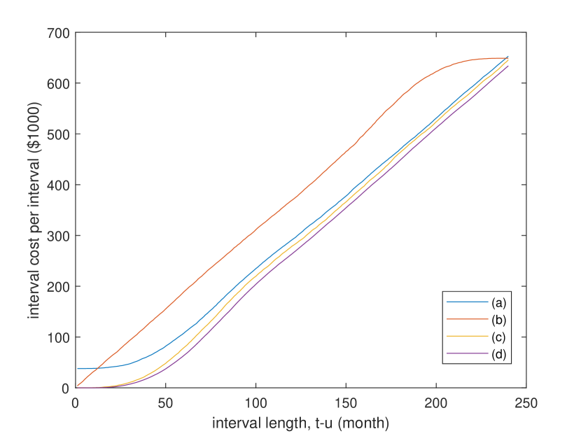
i Interval cost per interval as a function of the interval length $t-u$

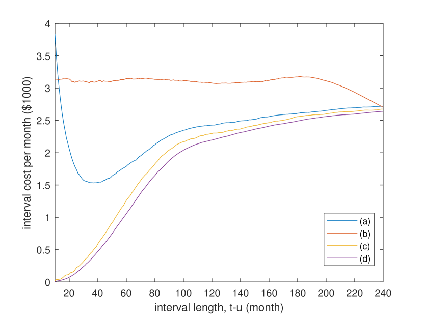
ii Interval cost per month as a function of the interval length $t-u$

Figure 2: Comparison of interval costs for the gearbox during different phases of time: Each interval starts at a PM occasion and ends at the (a) next PM occasion; (b)–(d) end of the planning period, which is (b) long before the end of the contract as well as the end of life; (c) at the end of the contract; (d) at the end of life.

For interval cost type (b), at the end of the interval, there is still a long contract period as well as component life left. Figure 2(2i) reveals that the interval cost type (b) is significantly higher than those of types (c) and (d), which is due to the gearbox being old with a high risk of break-down and that interval cost type (b) takes into account the age of the gearbox also after time step $t$. For long intervals (i.e., when $t-u$ is close to $T$), the wind farm’s age is close to its end of life. Hence, $c_{ut}^{ij}$ is close to $C_{ut}^{ij}$, i.e., the interval costs of type (b) tend to those of type (c) for long intervals. When $t$ is at the end of the planning period, it holds that $\check{C}_{ut}^{ij}<C_{ut}^{ij}$ for all $u<t$, which is due to the fact that if the gearbox breaks too close to the end of its life, maintenance will not be beneficial; as a result of not performing maintenance, production will be lost. For any $u<t<{e_{\text{c}}}$, i.e., when $t$ denotes a PM occasion, the inequalities $C_{ut}^{ij}>C_{{e_{\text{c}}}-t+u,{e_{\text{c}}}}^{ij}$ and $c_{ut}^{ij}>C_{{e_{\text{c}}}-t+u,{e_{\text{c}}}}^{ij}$ hold, because PM costs need to be paid at PM occasions but not at the end of the contract period (i.e., at time step ${e_{\text{c}}}$). However, with an increasing probability of a breakdown before the scheduled PM activity, the difference between these costs decreases.

Figure 2(2ii) shows that for the gearbox and interval cost type (a), i.e., the interval ends at a PM occasion, the maintenance cost per month is the lowest at the interval length $t-u=38$ (months). For interval cost type (b), when $t-u$ approaches $T$, the probability of a breakdown during the time interval $[t,T]$ tends to $0$; hence, the monthly maintenance cost tends to the interval cost type (c). For interval costs type (c) and type (d), the monthly maintenance costs sometimes increase faster than the corresponding cost type (b); hence, it may be beneficial to employ a longer planning period for type (b) than for type (c) or type (d).

5.2 Case study 1: A ten years full service production-based maintenance contract

We consider a full service production-based maintenance contract, i.e., [C-I], over ten years, i.e., $120$ months, in phase [P-ii]. Our aim is to find the most beneficial scheduling, in terms of in which months the maintenance (i.e., replacement) of the different components should be performed.

The optimal PM schedules are presented in Table 2. All components are planned for PM during months $42$ and $85$, with an optimal total cost for maintenance of $\$4147000$. Then, when doubling the costs $c_{j}^{\text{\tiny PM}}$, the optimal schedule alters to comprise PM of all components only once, in month $66$, with an optimal total cost of $\$5525000$.

$c_{j}^{\text{\tiny PM}}$, $j\in\mathcal{J}$	Planned PM for components [month]				Total cost	Computing
$[\$1000]$	Rotor	Main bearing	Gearbox	Generator	$[\$1000]$	times [s]
28  15  38  25	42 85	42 85	42 85	42 85	4147	60+0.53
56  30  76  50	66	66	66	66	5525	62+0.24

Table 2: Optimal schedules (months) for planned PM from the model (11), over a planning period of $10$ years, i.e., $120$ months, for $f_{t}=\$50000$ and two levels of the costs $c_{j}^{\text{\tiny PM}}$, $j\in\mathcal{J}$. Computing times represent the calculation of model parameters using Matlab ($60$ s and $62$ s, respectively)vand solving the model using CPLEX ($0.53$ s and $0.24$ s, respectively)

We next compare the model (11) over ten years with the pure CM strategy defined in Section 3.2.4, in which maintenance is performed only when a component fails, a constant interval (CI) policy developed in [17], and the PMSPIC model developed in [9]. As reported in Table 3, for the pure CM strategy, the total maintenance cost is $\$6897000$, which is $66~{}\%$ higher than that of our optimal schedule; for the CI policy, the total cost for maintenance is around $\$5966000$, which is $39~{}\%$ higher than the optimal schedule; the total maintenance cost resulting from the PMSPIC model is around $\$4948000$, which is $20~{}\%$ higher than that of our optimal schedule.

Planning method	Total costs	Relative	Downtime	Availability
	[$\$1000$]	total costs	[months]	[$\%$]
Model (11)	4147	1	1.41	98.7
Pure CM strategy	6897	1.66	3.75	96.9
CI policy	5762	1.39	1.54	98.6
PMSPIC	4948	1.20	1.46	98.7

Table 3: Total costs ($\$1000$) and relative total costs for maintenance, average downtime (month), and technical availability level ($\%$), during 10 years for the four maintenance policies, with the mobilization costs $d_{t}=\$0$ and $f_{t}=\$50000$.

The resulting technical availability from each of the four methods is also presented in Table 3. For the pure CM strategy (with no planned PM), the average number of failures for one wind turbine over 10 years is $3.75$, meaning that the average downtime for each wind turbine is $3.75$ months. Applying the model (11) results in an average number of failures per turbine is $1.24$, this is due to the property of the model to result in more PM occasions when the probability of a component failure increases. Combined with two scheduled PM activities for each of the ten turbines, the average downtime for each wind turbine is $1.57$ months, which is less than half of the downtime under the pure CM strategy.

The technical availability resulting from the model (11) is thus considerably higher than that of the pure CM strategy, while also generating a substantially lower cost. Comparing with the CI policy and the PMSPIC model, the technical availability is approximately the same, but the total maintenance cost resulting from either of these two methods is considerably higher. From the comparison of these four methods, we conclude that the model (11) yields the highest technical availability at the lowest total cost for maintenance during ten years.

Nowadays, it is common to have a $97~{}\%$ production-based availability guarantee. With the three PM methods, the expected level of availability is around $98.7~{}\%$, while with the pure CM strategy, the expected level of availability is below $97~{}\%$. Hence, we conclude that planning for PM will provide great benefits by its ability to provide a substantially increased technical availability level.

5.3 Case study 2: Lifetime planning with no insurance contract and sudden component failures

We next consider lifetime planning with sudden component failures. The failures are sampled from the Weibull distribution, as defined in Table 1.

When a component fails, it has to undergo CM while the PM plan needs to be rescheduled from the point in time of the failure. The new schedule is then used until another component fails, at which time the PM plan is rescheduled. This process is repeated until the end of life of the wind farm.

We first plan PM for the ten turbines over a ten years maintenance period in phase [P-i]. Hence, the model (16a) is applied; the resulting PM schedule is presented in Table 4.

Turbine	Planned PM for components [month]				Cost	Computing
#	Rotor	Main bearing	Gearbox	Generator	$[\$1000]$	times [s]
1–10	39 78 120	39 78 120	39 78 120	39 78 120	5294/44.1	28+0.6

Table 4: Optimal schedule (months) for planned PM from the model (16a), over a planning period of $10$ years, i.e., during the months $1$–$120$. ’Cost’ denotes the ”total expected cost for performed and planned maintenance from month $1$”/”average expected cost per month for performed and planned maintenance”. ’Computing times’ represent calculation of model parameters using Matlab ($28$ s) and solving the model using CPLEX ($0.6$ s)

A gearbox break-down in turbine $1$ is then sampled at month $31$. The new PM schedule, calculated using the model (16a), is presented in Table 5. The total cost denotes the sum of costs for all PM and CM performed before the planning period, plus the cost of PM during the planning period at hand. Since the planned PM of gearbox $1$ in month $39$ is replaced by CM in month $31$, and after that all components receive PM three times during the planning period, the total cost of the new schedule is larger than that of the previously planned schedule (before the gearbox break-down). The total cost per month is, however, lower for the new schedule (i.e., $\$6029000/150\approx\$40200$) than for the previous schedule (i.e., $\$5294000/120\approx\$44100$).

Turbine	Planned PM for components [month]				Cost	Computing
#	Rotor	Main bearing	Gearbox	Generator	$[\$1000]$	times [s]
1	54 102 150	54 102 150	31 73 111 150	54 102 150	6029/40.2	98+18.6
2–10	54 102 150	54 102 150	39 73 111 150	54 102 150

Table 5: Optimal schedules (months) for planned PM from the model (16a)—with a sudden break of the gearbox of turbine $1$ in month $31$—over a planning period of $10$ years, i.e., during the months $31$–$150$. ’Cost’ denotes the ”total expected cost for performed and planned maintenance from month $1$”/”average expected cost per month for performed and planned maintenance”. ’Computing times’: calculating model parameters using Matlab ($98$ s); solving the model using CPLEX ($18.6$ s)

Then, a break-down is sampled of a main bearing in turbine $2$ in month $71$. The PM plan in Table 5 is thus followed until all the planned replacements in month $54$ are performed. Then, a new schedule is calculated from month $71$; it is presented in Table 6. The total cost $\$6655000$ equals the sum of costs for CM and PM already performed (i.e., CM of the gearbox in turbine $1$ in month $31$, and the performed PM in months $39$ and $54$ see Table 5), CM of the main bearing in month $71$, and the expected cost for all the planned PM (see Table 6).

Turbine	Planned PM for components [month]				Cost	Computing
#	Rotor	Main bearing	Gearbox	Generator	$[\$1000]$	times [s]
2	99 145 189	71 110 145 189	71 110 145 189	99 145 189	6655/35.0	171+72
1, 3–10	99 145 189	99 145 189	71 110 145 189	99 145 189

Table 6: Optimal schedules (months) for planned PM from the model (16a)—with a sudden break of the main bearing of turbine $2$ in month $71$—over $10$ years, i.e., months $71$–$190$. ’Cost’ denotes the ”total expected cost for performed and planned maintenance from month $1$”/”average expected cost per month for performed and planned maintenance”. ’Computing times’: calculating model parameters using Matlab ($171$ s); solving the model using CPLEX ($72$ s)

Then, a break-down is sampled of a rotor in turbine $3$ in month $131$. The PM plan in Table 6 is thus followed until all the planned replacements in month $110$ are performed. Then, a new schedule is calculated from month $131$ until the end of life of the wind farm, hence using the model (18). The resulting PM schedule is presented in Table 7. The total cost $\$7107000$ is the sum of costs for CM and PM already performed (i.e., CM of the gearbox in turbine $1$ in month $31$, CM of the main bearing of turbine $2$ in month $71$, and the performed PM in months $39$, $54$, $71$, $99$, and $110$, according to Tables 5–6), CM of the rotor in month $131$, and the expected cost for all the planned PM in months $150$ and $195$ (according to Table 7).

Turbine	Planned PM for components [month]				Cost	Computing
#	Rotor	Main bearing	Gearbox	Generator	$[\$1000]$	times [s]
3	131 195	150 195	150 195	150 195	7107/29.6	176+98
1–2, 4–10	150 195	150 195	150 195	150 195

Table 7: Optimal schedules (months) for planned PM from the model (18)—with a sudden break of a rotor of turbine $3$ in month $131$—for a planning period comprising the rest of the wind farm’s life, i.e., during months $131$–$240$. ’Cost’ denotes the ”total expected cost for performed and planned maintenance from month $1$”/”average expected cost per month for performed and planned maintenance”. ’Computing times’: calculating model parameters using Matlab ($176$ s); solving the model using CPLEX ($98$ s)

Then, a break-down is sampled of the generator of turbine $4$ in month $181$. The PM plan in Table 7 is thus followed until all the planned replacements in month $150$ are performed. Then, a new schedule is calculated from month $181$; it is presented in Table 8. The total cost $\$6463000$ is the sum of costs for CM and PM already performed (i.e., CM of the gearbox in turbine $1$ in month $31$, CM of the main bearing of turbine $2$ in month $71$, CM of the rotor of turbine $3$ in month $131$, and the performed PM in months $39$, $54$, $71$, $99$, $110$, and $150$, according to Tables 5–7), CM of the generator in month $181$, and all the planned PM in month $195$ (according to Table 8).

Turbine	Planned PM for components [month]				Cost	Computing
#	Rotor	Main bearing	Gearbox	Generator	$[\$1000]$	times [s]
4	195	195	195	181	6463/26.9	86+15
1–3, 5–10	195	195	195	195

Table 8: Optimal schedules (months) for planned PM from the model (18)—with a sudden break of the generator of turbine $4$ in month $181$—for a planning period comprising the rest of the wind farm’s life, i.e., during months $181$–$240$. ’Cost’ denotes the ”total expected cost for performed and planned maintenance from month $1$”/”average expected cost per month for performed and planned maintenance”. ’Computing times’: calculating model parameters using Matlab ($86$ s); solving the model using CPLEX ($15$ s)

Then, a break-down of the gearbox of turbine $5$ is sampled in month $235$. The PM plan in Table 8 is thus followed until all the planned replacements in month $195$ are performed. Since it is close to the end of life of the wind turbine, by comparing the production loss for one turbine during the five remaining months and the cost of CM, we conclude that it will not be beneficial to maintain this gearbox during month $235$.

The final total maintenance cost, including the downtime cost resulting from the updated PM plans at CM occasions, as well as the downtime cost of one turbine after the breakdown in month $235$, equals $\$5798000$, which corresponds to an average of $\$24200$ per month during the life of the wind farm. The expected number of breakdowns during this wind farm’s life—when following the PM plan—is larger than $20$. Due to not experiencing as many breakdowns as expected, the final total maintenance cost is thus lower than expected—compare with the numbers in Tables 7–8.

5.4 Case study 3: Lifetime planning with no insurance contract

We next consider a case with no insurance contract, i.e., a contract of type [C-III], over $20$ years, ($240$ months) during the phase [P-iii]. Hence, the model (18) is applied; the resulting PM schedule is presented in Table 9.

Planned PM for components [month]				Total cost	Computing
Rotor	Main bearing	Gearbox	Generator	$[\$1000]$	times [s]
49 99 148 198	49 99 148 198	39 78 119 159 198	49 99 148 198	9153	213+3.4

Table 9: Optimal schedules (months) for planned PM from the model (18), over a planning period of $20$ years, i.e., $240$ months. Computing times represent calculation of model parameters using Matlab ($213$ s) and solving the model using CPLEX ($3.4$ s)

The total maintenance cost over these $20$ years is $\$9153000$, which is larger than twice the maintenance cost, i.e., $\$4147000$ over ten years, as computed in Case study $1$ considering the phase [P-ii], the end of a full service production-based maintenance contract. Hence, at the end of phase [P-ii], even though the components are old, there is no additional cost for compensating age. Moreover, the total cost over $20$ years in phase [P-iii] is lower than twice the cost $\$5294000$ of the first ten years plan in Case study $2$, considering the phase [P-i]. This is due to the fact that at the end of life, the component ages need not be considered.

We then look further into the computational complexity of our models by redefining the time steps to comprise three days instead of one month, resulting in the number of time steps in the model being multiplied by ten; the resulting PM schedule is presented in Table 10.

Planned PM for components [3 days]				Total cost	Computing
Rotor	Main bearing	Gearbox	Generator	$[\$1000]$	times [min]
495 990 1486 1982	495 990 1486 1982	394 788 1190 1586 1982	495 990 1486 1982	9129	65+319

Table 10: Optimal schedules ($3$ days) for planned PM from the model (18), over a planning period of $20$ years, i.e., $240$ months. Computing times represent calculation of model parameters using Matlab ($65$ min) and solving the model using CPLEX ($319$ min)

Comparing with the results from employing time steps of one month, the schedules are refined, but essentially equivalent. Hence, the finer time discretization mainly lead to substantially increased computing times while the results are not improved. We conclude that the time steps of one month should be kept.

5.5 Case study $4$: Lifetime planning with a basic insurance contract

We next investigate the case when—at a component failure—with the probability $\delta\in[0,1]$ the insurance company will pay for a new component. Then the cost of a new component plus the logistics cost for the replacement, i.e., $b_{j}^{\tiny\text{\tiny CM}}$, is reduced by the probability times the component cost, i.e., $\delta g_{j}^{\tiny\text{\tiny CM}}$, according to the expressions in (19). We employ the values of $g_{j}^{\tiny\text{\tiny CM}}$ from Tian et al. [17, Table 2] and which are given by $\$112000$, $\$60000$, $\$152000$, and $\$100000$ for the rotor, the main bearing, the gearbox, and the generator, respectively.

Here we apply the modified version of model (18), with the cost defined in (17) altered analogously as the costs in the formula (19). For different values of $\delta\in\{1.0,0.8,0.6,0.4,0.2\}$, the optimization model yields the corresponding optimal PM schedules presented in Table 11. Note that for $\delta\in\{0.8,0.6\}$ the optimal schedules are equal and that also $\delta\in\{0.4,0.2\}$ yield equal optimal schedules. Note also that for large values of $\delta$—representing a high probability that the insurance company will pay for the component cost at a failure—the wind farm owner should plan for fewer PM activities, i.e., the number of planned PM occasions is non-increasing with an increasing value of $\delta$.

$\delta$	Planned PM for components [month]				$F^{*}(\delta)$
	Rotor	Main bearing	Gearbox	Generator	$[\$1000]$
1.0	90 181	90 181	90 181	90 181	5292
0.8	63 123 186	63 123 186	63 123 186	63 123 186	6471
0.6	63 123 186	63 123 186	63 123 186	63 123 186	7385
0.4	49 99 148 198	49 99 148 198	49 99 148 198	49 99 148 198	8054
0.2	49 99 148 198	49 99 148 198	49 99 148 198	49 99 148 198	8620

Table 11: Optimal schedules (months) for planned PM resulting from the modified version of model (18), for different values of $\delta\in[0,1]$, over a planning period of $20$ years, i.e., $240$ months. $F^{*}(\delta)$ denotes the total cost of maintenance during the $20$ years under a $\delta$-insurance contract

The optimal value of the lifetime PM schedule for the case when there is no insurance contract (i.e., for $\delta=0.0$), as presented in Table 9, equals $F^{*}(0)=\$9153000$.

We conclude that the benefit of planned PM depends on the terms of the insurance, and that a reasonable price of a $\delta$-insurance maintenance contract can be computed as the difference $F^{*}(0)\!-\!F^{*}(\delta)$.

6 Conclusion

This paper models the optimal planning of preventive maintenance (PM) for a wind farm. Our models take into account component failures and necessary corrective maintenance (CM) as well as the effect of the expected costs for CM on the PM planning. We provide optimization models for different kinds of contracts and during different phases of the life of the wind farm.

Case study $1$ reveals that, as applied to a full service production-based maintenance contract, a comparison of our model with a pure CM strategy, a constant interval policy, and a pure PM model, indicates that planning for PM while taking into account costs for expected CM provides a high technical availability level at a comparatively low cost for maintenance.

Case study $2$ concerns lifetime planning with no insurance contract, with a rescheduling of the PM plan each time a component breaks and CM is necessary, throughout the life of the wind farm. With only five sampled breakdowns, the eventual total cost for maintenance is lower than expected. Due to the low PM cost, when one component in one wind turbine breaks, it affects the PM plan only for that particular wind turbine, while the other turbines’ PM plans are mostly unaffected.

Case study $3$ reveals that when scheduling the maintenance during the entire life of the wind farm, the first PM occasions are almost equidistant while the intervals between the later PM occasions are shorter. This is explained in Section 5.1: for an increasing interval length the interval cost between (d) a PM occasion and the end of life, increases faster than that between (a) two PM occasions.

Since our optimization model is NP-hard (see [9]), the computing time is expected to increase exponentially with the problem size (in terms of numbers of variables and constraints). This property is confirmed in Case study $3$, where we investigate a finer (by a factor of ten) discretization of time.

Case study $4$ regards an insurance contract, under which an insurance company pays for part of the CM costs caused by (sudden) component failures; the insurance level is then modelled by a probability that the CM costs are paid by the insurance company. Our results show that the number of planned PM occasions for the wind farm decreases with an increasing insurance level. Further, the optimal costs for PM can be used to advise the wind farm owners what is a fair price of a certain level of an insurance contract.

The optimization models presented in this article regards PM scheduling and CM strategies for the stakeholders involved, i.e., wind farm owners, maintenance companies, and insurance companies. Solutions from these models can be used to guide on reasonable costs and prices for different types of contracts between the stakeholders during different phases of the life of a wind farm.

References

References

- [1] The Swedish Wind Power Technology Centre at Chalmers University of Technology in Gothenburg, Sweden.
-
[2]
CPLEX Optimizer v. 20.1.
https://www.ibm.com/analytics/cplex-
optimizer. IBM ILOG. - mat [2015] Matlab R2019b. https://www.mathworks.com/products/matlab.html, 2015. MathWorks.
- amp [2018] AMPL IDE v. 12.1,. http://www.ampl.com, 2018. AMPL Optimization LLC.
- win [2020a] U.S. Energy and Employment Report. https://www.usenergyjobs.org, 2020a. Accessed: 2021-01-08.
- win [2020b] Wind vision. https://www.energy.gov/eere/wind/maps/wind-vision, 2020b. Accessed: 2021-01-08.
- de Almeida [2001] A. T. de Almeida. Multicriteria decision making on maintenance: spares and contracts planning. European Journal of Operational Research, 129(2):235–241, 2001.
- Fulkerson [1966] D. R. Fulkerson. Flow networks and combinatorial operations research. The American Mathematical Monthly, 73(2):115–138, 1966.
- Gustavsson et al. [2014] E. Gustavsson, M. Patriksson, A.-B. Strömberg, A. Wojciechowski, and M. Önnheim. Preventive maintenance scheduling of multi-component systems with interval costs. Computers & Industrial Engineering, 76:390–400, 2014.
- Jafari et al. [2018] L. Jafari, F. Naderkhani, and V. Makis. Joint optimization of maintenance policy and inspection interval for a multi-unit series system using proportional hazards model. Journal of the Operational Research Society, 69(1):36–48, 2018.
- Lee and Cha [2016] H. Lee and J. H. Cha. New stochastic models for preventive maintenance and maintenance optimization. European Journal of Operational Research, 255(1):80–90, 2016.
- Lisnianski et al. [2008] A. Lisnianski, I. Frenkel, L. Khvatskin, and Y. Ding. Maintenance contract assessment for aging systems. Quality and Reliability Engineering International, 24(5):519–531, 2008.
- Moghaddam and Usher [2011] K. S. Moghaddam and J. S. Usher. Sensitivity analysis and comparison of algorithms in preventive maintenance and replacement scheduling optimization models. Computers & Industrial Engineering, 61(1):64–75, 2011.
- Park and Pham [2016] M. Park and H. Pham. Cost models for age replacement policies and block replacement policies under warranty. Applied Mathematical Modelling, 40(9–10):5689–5702, 2016.
- Qiu et al. [2017] Q. Qiu, L. Cui, J. Shen, and L. Yang. Optimal maintenance policy considering maintenance errors for systems operating under performance-based contracts. Computers & Industrial Engineering, 112:147–155, 2017.
- Rose [1929] L. Rose. Motorcoach maintenance. SAE Transactions, pages 659–670, 1929.
- Tian et al. [2011] Z. Tian, T. Jin, B. Wu, and F. Ding. Condition based maintenance optimization for wind power generation systems under continuous monitoring. Renewable Energy, 36(5):1502–1509, 2011.
- Tian et al. [2014] Z. Tian, B. Wu, and M. Chen. Condition-based maintenance optimization considering improving prediction accuracy. Journal of the Operational Research Society, 65(9):1412–1422, 2014.
- Yeh and Chen [2006] R. H. Yeh and C.-K. Chen. Periodical preventive-maintenance contract for a leased facility with Weibull life-time. Quality and Quantity, 40(2):303–313, 2006.
- Ziegler et al. [2018] L. Ziegler, E. Gonzalez, T. Gonzalez, U. Smolka, and J. J. Melero. Lifetime extension of onshore wind turbines: A review covering Germany, Spain, Denmark, and the UK. Renewable and Sustainable Energy Reviews, 82:1261–1271, 2018.