On Bisimilarities for Closure Spaces
Preliminary Version

Abstract

Closure spaces are a generalisation of topological spaces obtained by removing the idempotence requirement on the closure operator. We adapt the standard notion of bisimilarity for topological models, namely Topo-bisimilarity, to closure models—we call the resulting equivalence CM-bisimilarity—and refine it for quasi-discrete closure models. We also define two additional notions of bisimilarity that are based on paths on space, namely Path-bisimilarity and Compatible Path-bisimilarity, CoPa-bisimilarity for short. The former expresses (unconditional) reachability, the latter refines it in a way that is reminishent of Stuttering Equivalence on transition systems. For each bisimilarity we provide a logical characterisation, using variants of SLCS. We also address the issue of (space) minimisation via the three equivalences.

losure Spaces; Topological Spaces; Spatial Logics; Spatial Bisimilarities.

1 Introduction

In the well known topological interpretation of model logic a point in space satisfies formula $\diamond\,\Phi$ whenever it belongs to the topological closure of the set $[\![\Phi]\!]$ of all the points satisfying formula $\Phi$ (see e.g. [5]). Topological spaces form the fundamental basis for reasoning about space, but the idempotence property of topological closure turns out to be too restrictive. For instance, discrete structures useful for certain representations of space, like general graphs, cannot be captured. To that purpose, a more liberal notion of space, namely that of closure spaces, has been proposed in the literature that does not require idempotence of the closure operator (see [16] for an in-depth treatment of the subject).

In [11, 12] the Spatial Logic for Closure Spaces (${\tt SLCS}$) has been proposed that enriches modal logic with a surrounded operator $\mathcal{S}$ such that a point $x$ satisfies $\Phi_{1}\,\mathcal{S}\,\Phi_{2}$ if it lays in a set $A\subseteq[\![\Phi_{1}]\!]$ and the external border of which is composed by points in $[\![\Phi_{2}]\!]$, i.e. $x$ satisfies $\Phi_{1}$ and is surrounded by points satisfying $\Phi_{2}$. A model checking algorithm has been proposed in  [11, 12] that has been implemented in the tool topochecker [9, 10] and, more recently, in VoxLogicA [4], a tool specialised for spatial model-checking digital images, that can be modelled as adjacency spaces, a special case of closure spaces.

The logic and its model checkers have been applied to several case studies [12, 10, 9] including a declarative approach to medical image analysis [4, 3, 8, 2]. An encoding of the discrete Region Connection Calculus RCC8D of [22] into the collective variant of SLCS has been proposed in [13]. The logic has also inspired other approaches to spatial reasoning in the context of signal temporal logic and system monitoring [1, 21] and in the verification of cyber-physical systems [23]. In [19] it has been shown that SLCS cannot express topological separation and connectedness; the authors propose a notion of path preserving bisimulation.

A key question, when reasoning about modal logics and their models, is the relationship between logical equivalences and notions of bisimilarity defined on their underlying models. This is also important because the existence of such bisimilarities, and their logical characterisation, makes it possible to exploit minimisation procedures for bisimilarity for the purpose of efficient model-checking.

In this paper we study three different notions of bisimilarity for closure models, i.e. models based on closure spaces. The first one is CM-bisimilarity, that is an adaptation for closure models of classical Topo-bisimilarity for topological models [5]. Actually, CM-bisimilarity is an instantiation to closure models of Monotonic bisimulation on neighbourhood models [6, 18]. In fact, it is defined using the interior operator of closure models, that is monotonic, thus making closure models an intantiation of monotonic neighbourhood models. We show that CM-bisimilarity is weaker than homeomorphism and provide a logical characterisation of the former, namely the Infinitary Modal Logic.

We then present a refinement of CM-bisimilarity, specialised for quasi-discrete closure models, i.e. closure models where every point has a minimal neighbourhood. In this case, the closure of a set of points—and so also its interior—can be expressed using an underlying binary relation; this gives raise to both a direct closure and interior of a set, and a converse closure and interior, the latter being obtained using the inverse of the binary relation. This, in turn, induces a refined notion of bisimilarity, CM-bisimilarity with converse, which, on quasi-discrete closure models, is shown to be strictly stronger than CM-bisimilarity. We also introduce a notion of Trace Equivalence for closure models and show that CM-bisimilarity with converse implies Trace Equivalence, but not the other way around.

We extend the Infinitary Modal Logic with the converse of its unary modal operator and show that the resulting logic characterises CM-bisimilarity with converse. CM-bisimulation with converse, as CM-bisimulation, is defined using the interior operator, $\mathcal{I}$. We show that $\mathcal{C}$-bisimulation, proposed in [14], and resembling Strong Back-and-Forth bisimilarity for processes proposed in [15], coincides with CM-bisimulation with converse. The definition of $\mathcal{C}$-bisimulation uses the closure operator $\mathcal{C}$, i.e. the dual of $\mathcal{I}$. The advantage of using directly the closure operator, which is the foundational operator of closure spaces, is given by its intuitive interpretation in quasi-discrete closure models that makes several proofs simpler. We recall here that in [14] a minimisation algorithm for $\mathcal{C}$-bisimulation, and related tool, MiniLogicA, have been proposed as well. We show that the infinitary extension ISLCS of (a variant of) SLCS, fully characterises $\mathcal{C}$-bisimulation. The variant of SLCS of interest here is the one with two modal operators expressing (conditional) reachability. More specifically, one operator expresses the possibility that a point in space may reach an area satisfying a given formula $\Phi_{1}$ via a path the points of which satisfy a formula $\Phi_{2}$; the other expresses the possibility that a point in space may be reached from an area satisfying a given formula $\Phi_{1}$ via a path the points of which satisfy a formula $\Phi_{2}$. The classical Infinitary Modal Logic modal operator, and its converse, can be derived from the reachability operators of SLCS, when the underlying model is quasi-discrete. This last result brings to the coincidence of CM-bisimilarity with converse and $\mathcal{C}$-bisimilarity for quasi-discrete closure models.

CM-bisimilarity, and CM-bisimilarity with converse, play an important role as they are the counterpart of classical Topo-bisimilarity. On the other hand, they turn out to be rather too strong when one has in mind intuitive relations on space like, e.g. scaling, that may be useful when dealing with models representing images (see [8, 2, 4, 3] for details). For this purpose, we introduce our second, weaker notion of bisimilarity, namely Path-bisimulation that is essentially based on reachability of bisimilar points by means of paths over the underlying space. We show that, for quasi-discrete closure models, Path-bisimilarity is strictly weaker than CM-bisimilarity with converse; we also show that a similar result does not hold for general CM-bisimilarity and general closure models. We provide a remedy to such problem, for the case in which the space is path-connected, using an adaptation for CMs of INL-bisimilarity [6]. We furthermore show that Path-bisimilarity and Trace Equivalence for general CMs are uncomparable. We finally consider the Infinitary Modal Logic where the modal operator is replaced by two unary modalities—one for (unconditional) reachability of an area satisfying a given formula, and the other for (unconditional) reachability from an area satisfying a given formula—and prove that such a logic characterises Path-bisimilarity.

Path-bisimilarity is in some sense too weak, abstracting too much; nothing whatsoever is required of the relevant paths, except their starting points being fixed and related by the bisimulation, and their end-points be in the bisimulation as well. A little bit deeper insight into the structure of such paths would be desirable as well as some, relatively high level, requirements on them. To that purpose we resort to a notion of “compatibility” between relevant paths that essentially requires each of them to be composed by a sequence of non-empty “zones”, with the total number of zones in each of the two paths being the same, while the length of each zone being arbitrary (but at least 1); each element of one path in a given zone is required to be related by the bisimulation to all the elements in the corresponding zone in the other path. This idea of compatibility gives rise to the third notion of bisimulation, namely Compatible Path bisimulation, CoPa-bisimulation, which is strictly stronger than Path-bisimilarity and, for quasi-discrete closure models, strictly weaker than CM-bisimilarity with converse. We also show that Compatible Path bisimulation and Trace Equivalence are uncomparable and we provide a logical characterisation of Compatible Path bisimulation using a restricted version of ISLCS. The notion of CoPa-bisimulation is reminiscent of that of the Equivalence with respect to Stuttering for transition systems proposed in [7], although in a different context and with different definitions as well as underlying notions.

The paper is organised as follows: after having settled the context and offered some preliminary notions and definitions in Section 2, in Section 3 we present CM-bisimilarity. Section 4 deals with CM-bisimulation with converse. Section 5 addresses Path-bisimilarity, while in Section 6 CoPa-bisimilarity is dealt with. We conclude the paper with Section 7. All detailed proofs are provided in the Appendix.

2 Preliminaries

In this paper, given set $X$, $\mathbf{\mathcal{P}}(X)$ denotes the powerset of $X$; for $Y\subseteq X$ we let $\overline{Y}$ denote $X\setminus Y$, i.e. the complement of $Y$. For function $f:X\to Y$ and $A\subseteq X$, we let $f(A)$ be defined as $\{f(a)\,|\,a\in A\}$. For binary relation $R\subseteq X\times X$ we let $R^{-1}$ denote the relation $\{(x_{1},x_{2})\,|\,(x_{2},x_{1})\in R\}$, whereas $R^{r}$ ($R^{s}$, respectively) will denote the transitive closure (symmetric closure, respectively) of $R$, and $R^{rst}$ will denote the reflexive, symmetric and transitive closure of $R$. In this section, we recall several definitions and results on closure spaces, most of which are taken from [16].

Definition 1 (Closure Space - CS)

A closure space, CS for short, is a pair $(X,\mathcal{C})$ where $X$ is a non-empty set (of points) and $\mathcal{C}:\mathbf{\mathcal{P}}(X)\to\mathbf{\mathcal{P}}(X)$ is a function satisfying the following axioms:

1. $\mathcal{C}(\emptyset)=\emptyset$;

2. $A\subseteq\mathcal{C}(A)$ for all $A\subseteq X$;

3. $\mathcal{C}(A_{1}\cup A_{2})=\mathcal{C}(A_{1})\cup\mathcal{C}(A_{2})$ for all $A_{1},A_{2}\subseteq X$. $\bullet$

It is worth pointing out that topological spaces coincide with the sub-class of CSs for which also the idempotence axiom $\mathcal{C}(\mathcal{C}(A)=\mathcal{C}(A)$ holds. The interior operator is the dual of closure: $\mathcal{I}(A)=\overline{\mathcal{C}(\overline{A})}$. A neighbourhood of a point $x\in X$ is any set $A\subseteq X$ such that $x\in\mathcal{I}(A)$. A minimal neighbourhood of a point $x$ is a neighbourhood $A$ of $x$ such that $A\subseteq A^{\prime}$ for any other neighbourhood $A^{\prime}$ of $x$.

We recall here the fact that the closure and, consequently, the interior operators are monotonic: if $A_{1}\subseteq A_{2}$ then $\mathcal{C}(A_{1})\subseteq\mathcal{C}(A_{2})$ and $\mathcal{I}(A_{1})\subseteq\mathcal{I}(A_{2})$.

Definition 2 (Quasi-discrete CS - QdCS)

A quasi-discrete closure space is a CS $(X,\mathcal{C})$ such that any of the following equivalent conditions holds:

1. each $x\in X$ has a minimal neighbourhood;

2. for each $A\subseteq X$ it holds that $\mathcal{C}(A)=\bigcup_{x\in A}\mathcal{C}(\{x\})$. $\bullet$

Given a relation $R\subseteq X\times X$, let function $\mathcal{C}_{R}:\mathbf{\mathcal{P}}(X)\to\mathbf{\mathcal{P}}(X)$ be defined as follows: for all $A\subseteq X$, $\mathcal{C}_{R}(A)=A\cup\{x\in X\,|\,\mbox{there exists }a\in A\mbox{ s.t. }(a,x)\in R\}.$ It is easy to see that, for any $R$, $\mathcal{C}_{R}$ satisfies all the axioms of Definition 1 and so $(X,\mathcal{C}_{R})$ is a CS. The following theorem is a standard result in the theory of CSs [16]:

Theorem 2.1

A CS $(X,\mathcal{C})$ is quasi-discrete if and only if there is a relation $R\subseteq X\times X$ such that $\mathcal{C}=\mathcal{C}_{R}$. ∎

In the sequel, whenever $(X,\mathcal{C})$ is quasi-discrete, we will let $\stackrel{{\scriptstyle\rightarrow}}{{\mathcal{C}}}$ denote $\mathcal{C}_{R}$, and, consequently, we will let $(X,\stackrel{{\scriptstyle\rightarrow}}{{\mathcal{C}}})$ denote the space, abstracting from the specification of relation $R$, when the latter is not necessary. Moreover, we will let $\stackrel{{\scriptstyle\leftarrow}}{{\mathcal{C}}}$ denote $\mathcal{C}_{R^{-1}}$. $\stackrel{{\scriptstyle\rightarrow}}{{\mathcal{I}}}$ and $\stackrel{{\scriptstyle\leftarrow}}{{\mathcal{I}}}$ are defined in the obvious way: $\stackrel{{\scriptstyle\rightarrow}}{{\mathcal{I}}}A=\overline{\stackrel{{\scriptstyle\rightarrow}}{{\mathcal{C}}}(\overline{A})}$ and $\stackrel{{\scriptstyle\leftarrow}}{{\mathcal{I}}}A=\overline{\stackrel{{\scriptstyle\leftarrow}}{{\mathcal{C}}}(\overline{A})}$.

An example of the difference between $\stackrel{{\scriptstyle\rightarrow}}{{\mathcal{C}}}$ and $\stackrel{{\scriptstyle\leftarrow}}{{\mathcal{C}}}$ is shown in Figure 1.

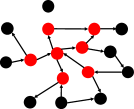
(a)

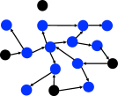
(b)

(c)

Figure 1: Given the points satisfying $\Phi$, shown in red in Fig. 1a, those satisfying $\stackrel{{\scriptstyle\rightarrow}}{{\mathcal{C}}}(\Phi)$ are shown in blue in Fig. 1b and those satisfying $\stackrel{{\scriptstyle\leftarrow}}{{\mathcal{C}}}(\Phi)$ are shown in blue in Fig. 1c

In the context of the present paper, paths over closure spaces play an important role; therefore, we give a formal definition of paths as continuous functions below.

Definition 3 (Continuous function)

Function $f:X_{1}\to X_{2}$ is a continuous function from $(X_{1},\mathcal{C}_{1})$ to $(X_{2},\mathcal{C}_{2})$ if and only if for all sets $A\subseteq X_{1}$ we have: $f(\mathcal{C}_{1}(A))\subseteq\mathcal{C}_{2}(f(A))$. $\bullet$

Definition 4 (Connected space)

Given CS $(X,\mathcal{C})$, $A\subseteq X$ is connected if it is not the union of two non-empty separated sets. $A_{1},A_{2}\subseteq X$ are separated if $A_{1}\cap\mathcal{C}(A_{2})=\mathcal{C}(A_{1})\cap A_{2}=\emptyset$. $(X,\mathcal{C})$ is connected if $X$ is connected. $\bullet$

Definition 5 (Index space)

An index space is a connected CS $(I,\mathcal{C})$ equipped with a total order $\leq\subseteq I\times I$ with a bottom element $0$. We write $\iota_{1}<\iota_{2}$ whenever $\iota_{1}\leq\iota_{2}$ and $\iota_{1}\not=\iota_{2}$. $\bullet$

Definition 6 (Path)

A path in CS $(X,\mathcal{C})$ is a continuous function from an index space $\mathcal{J}=(I,\mathcal{C}^{\mathcal{J}})$ to $(X,\mathcal{C})$. Path $\pi$ is bounded if there exists $\ell\in I$ s.t. $\pi(\iota)=\pi(\ell)$ for all $\iota$ such that $\ell\leq\iota$; we call $\ell$ the length of $\pi$, written $\mathtt{len}(\pi)$.

For bounded path $\pi$ we define the domain of $\pi$, $\mathtt{dom}(\pi)$, as the set $\{\iota\,|\,\iota\leq\mathtt{len}(\pi)\}$ and $\mathtt{range}(\pi)=\{\pi(\iota)\,|\,\iota\leq(\mathtt{len}\,\pi)\}$ (the range of $\pi$). $\bullet$

Of particular importance in the present paper are quasi-discrete paths and Euclidean paths. Quasi-discrete paths are paths having $(\mathbb{N},\mathcal{C}_{\mathtt{succ}})$ as index space, where $\mathbb{N}$ is the set of natural numbers and $\mathtt{succ}$ is the successor relation $\mathtt{succ}=\{(m,n)\,|\,n=m+1\}$. The index space of Euclidean paths is instead the set of non-negative real numbers equipped with the classical closure operator.

Proposition 1

For all QdCS $(X,\stackrel{{\scriptstyle\rightarrow}}{{\mathcal{C}}}),A,A_{1},A_{2}\subseteq X,x_{1},x_{2}\in X$, and function $\pi:\mathbb{N}\to X$ the following holds:

1. $\stackrel{{\scriptstyle\leftarrow}}{{\mathcal{C}}}(A)=A\cup\{x\in X\,|\,\mbox{there exists }a\in A\mbox{ such that }(x,a)\in R\}$;

2. $x_{1}\in\stackrel{{\scriptstyle\leftarrow}}{{\mathcal{C}}}(\{x_{2}\})$ if and only if $x_{2}\in\stackrel{{\scriptstyle\rightarrow}}{{\mathcal{C}}}(\{x_{1}\})$;

3. $\stackrel{{\scriptstyle\leftarrow}}{{\mathcal{C}}}(A)=\{x\,|\,x\in X\mbox{ and exists }a\in A\mbox{ such that }a\in\stackrel{{\scriptstyle\rightarrow}}{{\mathcal{C}}}(\{x\})\}$;

4. if $A_{1}\subseteq A_{2}$, then $\stackrel{{\scriptstyle\leftarrow}}{{\mathcal{C}}}(A_{1})\subseteq\,\stackrel{{\scriptstyle\leftarrow}}{{\mathcal{C}}}(A_{2})$ and $\stackrel{{\scriptstyle\leftarrow}}{{\mathcal{I}}}(A_{1})\subseteq\,\stackrel{{\scriptstyle\leftarrow}}{{\mathcal{I}}}(A_{2})$.

5. $\pi$ is a path over $X$ if and only if for all $i\in\mathtt{dom}(\pi)\setminus\{0\}$, the following holds:
   $\pi(i)\in\stackrel{{\scriptstyle\rightarrow}}{{\mathcal{C}}}(\pi(i-1))$ and $\pi(i-1)\in\stackrel{{\scriptstyle\leftarrow}}{{\mathcal{C}}}(\pi(i))$.

Remark 1

Note that the definition of the closure operator for QdCSs given in [16] coincides with $\stackrel{{\scriptstyle\leftarrow}}{{\mathcal{C}}}A$, as given in the first item of Proposition 1.

In the sequel we fix a set ${\tt AP}$ of atomic proposition letters.

Definition 7 (Closure model - CM)

A closure model, CM for short, is a tuple $\mathcal{M}=(X,\mathcal{C},\mathcal{V})$, with $(X,\mathcal{C})$ a CS, and $\mathcal{V}:{\tt AP}\to\mathbf{\mathcal{P}}(X)$ the (atomic predicate) valuation function assigning to each $p\in{\tt AP}$ the set of points where $p$ holds. $\bullet$

The following definition adapts the notion of homeomorphism for topological spaces, as given in [20], to the case of closure spaces.

Definition 8 (Homeomorphism)

A homeomorphism between CMs $\mathcal{M}_{1}=(X_{1},\mathcal{C}_{1},\mathcal{V}_{1})$ and $\mathcal{M}_{2}=(X_{2},\mathcal{C}_{2},\mathcal{V}_{2})$ is a bijection $h:X_{1}\to X_{2}$ s.t. for all $x_{1}\in X_{1}$, $x_{2}\in X_{2},A_{1}\subseteq X_{1}$ and $A_{2}\subseteq X_{2}$, the following holds:

1. $\mathcal{V}^{-1}_{1}(x_{1})=\mathcal{V}^{-1}_{2}(h(x_{1}))$;

2. $\mathcal{V}^{-1}_{2}(x_{2})=\mathcal{V}^{-1}_{1}(h^{-1}(x_{2}))$;

3. $h(\mathcal{I}_{1}(A_{1}))=\mathcal{I}_{2}(h(A_{1}))$;

4. $h^{-1}(\mathcal{I}_{2}(A_{2}))=\mathcal{I}_{1}(h^{-1}(A_{2}))$.

We say that $x_{1},x_{2}\in X$ are homeomorphic, written $x_{1}\rightleftharpoons_{\mathtt{HO}}x_{2}$ if and only if there is an homeomorphism $h$ such that $x_{2}=h(x_{1})$. $\bullet$

An alternative, equivalent, definition can be obtained by requiring that $h(\mathcal{C}_{1}(A_{1}))$ $=$ $\mathcal{C}_{2}(h(A_{1}))$ and $h^{-1}(\mathcal{C}_{2}(A_{2}))=\mathcal{C}_{1}(h^{-1}(A_{2}))$ instead of $h(\mathcal{I}_{1}(A_{1}))=\mathcal{I}_{2}(h(A_{1}))$ and $h^{-1}(\mathcal{I}_{2}(A_{2}))=\mathcal{I}_{1}(h^{-1}(A_{2}))$.

All the definitions given above for CSs apply to CMs as well; thus, a quasi-discrete closure model (QdCM for short) is a CM $\mathcal{M}=(X,\stackrel{{\scriptstyle\rightarrow}}{{\mathcal{C}}},\mathcal{V})$ where $(X,\stackrel{{\scriptstyle\rightarrow}}{{\mathcal{C}}})$ is a QdCS. For model $\mathcal{M}=(X,\mathcal{C},\mathcal{V})$ we will often write $x\in\mathcal{M}$ when $x\in X$; similarly we will speak of paths in $\mathcal{M}$ meaning paths in $(X,\mathcal{C})$; we let $\mathtt{Paths}_{\mathcal{J},\mathcal{M}}$ denote the set of all paths in $\mathcal{M}$ with index space $\mathcal{J}$. $\mathtt{BPaths}_{\mathcal{J},\mathcal{M}}$ denotes the set of all bounded paths in $\mathcal{M}$, whereas for $x\in X$, $\mathtt{BPaths^{F}}_{\mathcal{J},\mathcal{M}}(x)$ denotes the set $\{\pi\in\mathtt{BPaths}_{\mathcal{J},\mathcal{M}}\,|\,\pi(0)=x\}$ and, similarly, $\mathtt{BPaths^{T}}_{\mathcal{J},\mathcal{M}}(x)$ denotes the set $\{\pi\in\mathtt{BPaths}_{\mathcal{J},\mathcal{M}}\,|\,\pi(\mathtt{len}(\pi))=x\}$. We will refrain from writing the subscripts _J,M whenever not necessary.

We often write $x\stackrel{{\scriptstyle\pi}}{{\Longrightarrow}}x^{\prime}$ if $\pi\in\mathtt{BPaths^{F}}_{\mathcal{J},\mathcal{M}}(x)\cap\mathtt{BPaths^{T}}_{\mathcal{J},\mathcal{M}}(x^{\prime})$ and $x\stackrel{{\scriptstyle}}{{\Longrightarrow}}x^{\prime}$ if there exists $\pi$ s.t. $x\stackrel{{\scriptstyle\pi}}{{\Longrightarrow}}x^{\prime}$. We say that $\mathcal{M}$ is path-connected if for all $x,x^{\prime}\in\mathcal{M}$ we have $x\stackrel{{\scriptstyle}}{{\Longrightarrow}}x^{\prime}$.

Finally, for $\pi\in\mathtt{Paths}_{\mathcal{J},\mathcal{M}}$ with $\mathcal{J}=(I,\mathcal{C}^{\mathcal{J}})$, we let $\mathtt{Tr}(\pi)$ denote the trace of $\pi$, namely $\mathtt{Tr}:\mathtt{Paths}_{\mathcal{J},\mathcal{M}}\to(I\to\mathbf{\mathcal{P}}({\tt AP}))$ with $\mathtt{Tr}(\pi)(\iota)=\mathcal{V}^{-1}(\pi(\iota))$. We say that $x_{1},x_{2}\in\mathcal{M}$ are trace equivalent, written $x_{1}\,\rightleftharpoons_{\mathtt{Tr}}\,x_{2}$ if $\mathtt{Tr}(\mathtt{BPaths^{F}}(x_{1}))=\mathtt{Tr}(\mathtt{BPaths^{F}}(x_{2}))$ and $\mathtt{Tr}(\mathtt{BPaths^{T}}(x_{1}))=\mathtt{Tr}(\mathtt{BPaths^{T}}(x_{2}))$.

In the sequel, for logic $\mathcal{L}$, formula $\Phi\in\mathcal{L}$, and model $\mathcal{M}=(X,\mathcal{C},\mathcal{V})$ we let $[\![\Phi]\!]^{\mathcal{M}}_{\mathcal{L}}$ denote the set $\{x\in X\,|\,\mathcal{M},x\models_{\mathcal{L}}\Phi\}$ of all the points in $\mathcal{M}$ that satisfy $\Phi$, where $\models_{\mathcal{L}}$ is the satisfaction relation for $\mathcal{L}$. For the sake of readability, we will refrain from writing the subscript _L when this will not cause confusion.

3 CM-bisimilarity

3.1 CM-bisimilarity

The first notion of bisimilarity that we consider is CM-bisimilarity. This notion stems from a natural adaptation for CMs of Topo-bisimilation for topological models, as defined e.g. in [5]. We recall such definition below, where $(X,\tau,\mathcal{V})$ is the topological model with set of points $X$, open sets $\tau$, and atomic predicate evaluation function $\mathcal{V}$:

Definition 9 (Topo-bisimulation)

A topological bisimulation or simply a topo-bisimulation between two topo-models $\mathcal{M}_{1}=(X_{1},\tau_{1},\mathcal{V}_{1})$ and $\mathcal{M}_{2}=(X_{2},\tau_{2},\\ \mathcal{V}_{2})$ is a non-empty relation $T\subseteq X_{1}\times X_{2}$ such that if $(x_{1},x_{2})\in T$ then:

1. $x_{1}\in\mathcal{V}_{1}(p)$ if and only if $x_{2}\in\mathcal{V}_{2}(p)$ for each $p\in{\tt AP}$;

2. (forth): $x_{1}\in U_{1}\in\tau_{1}$ implies there exists $U_{2}\in\tau_{2}$ such that $x_{2}\in U_{2}$ and for all $x_{2}^{\prime}\in U_{2}$ there exists $x_{1}^{\prime}\in U_{1}$ such that $(x_{1}^{\prime},x_{2}^{\prime})\in T$;

3. (back): $x_{2}\in U_{2}\in\tau_{2}$ implies there exists $U_{1}\in\tau_{1}$ such that $x_{1}\in U_{1}$ and for all $x_{1}^{\prime}\in U_{1}$ there exists $x_{2}^{\prime}\in U_{2}$ such that $(x_{1}^{\prime},x_{2}^{\prime})\in T$. $\bullet$

In the context of CMs, we replace the notion of open set containing a given point $x$ with that of neighbourhood of $x$, so that we get the following

Definition 10 (CM-bisimilarity)

Given CM $\mathcal{M}=(X,\mathcal{C},\mathcal{V})$, a non empty relation $B\subseteq X\times X$ is a CM-bisimulation over $X$ if, whenever $(x_{1},x_{2})\in B$, the following holds:

1. $\mathcal{V}^{-1}(x_{1})=\mathcal{V}^{-1}(x_{2})$;

2. for all neighbourhoods $S_{1}$ of $x_{1}$ there is a neighbourhood $S_{2}$ of $x_{2}$ such that for all $s_{2}\in S_{2}$, there is $s_{1}\in S_{1}$ with $(s_{1},s_{2})\in B$;

3. for all neighbourhoods $S_{2}$ of $x_{2}$ there is a neighbourhood $S_{1}$ of $x_{1}$ such that for all $s_{1}\in S_{1}$, there is $s_{2}\in S_{2}$ with $(s_{1},s_{2})\in B$.

$x_{1}$ and $x_{2}$ are CM-bisimilar, written $x_{1}\,\rightleftharpoons_{\mathtt{CM}}^{\mathcal{M}}\,x_{2}$, if and only if there is a CM-bisimulation $B$ over $X$ such that $(x_{1},x_{2})\in B$. $\bullet$

The above definition is very similar to that of bisimilarity between monotonic neighbourhood spaces [6, 18], and, in fact, monotonicity of the $\mathcal{I}$ operator makes it legitimate to interpret CMs as an instantiation of the notion of monotonic neighbourhood models (see [6, 18] for details).

CM-bisimilarity is coarser than homeomorphism:

Proposition 2

For all CMs $\mathcal{M}=(X,\mathcal{C},\mathcal{V})$ and $x_{1},x_{2}\in X$ the following holds: $x_{1}\,\rightleftharpoons_{\mathtt{HO}}\,x_{2}$ implies $x_{1}\,\rightleftharpoons_{\mathtt{CM}}\,x_{2}$.

The converse of Proposition 2 does not hold as shown in Figure 2 where $\mathcal{V}^{-1}(x_{11})=\mathcal{V}^{-1}(x_{21})=\{r\}\not=\{b\}=\mathcal{V}^{-1}(x_{12})=\mathcal{V}^{-1}(x_{22})=\mathcal{V}^{-1}(x_{23})$ and $x_{11}\rightleftharpoons_{\mathtt{CM}}x_{21}$ but $x_{11}\not\rightleftharpoons_{\mathtt{HO}}x_{21}$ (see Remark 3 in Appendix 0.B).

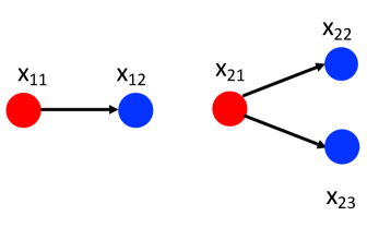
Figure 2: $x_{11}\rightleftharpoons_{\mathtt{CM}}x_{21}$ but $x_{11}\not\rightleftharpoons_{\mathtt{HO}}x_{21}$.

3.2 Logical Characterisation of CM-bisimilarity

In this section, we show that CM-bisimilarity is characterised by the Infinitary Modal Logic, IML for short. We first recall the definition of IML.

Definition 11 (Infinitary Modal Logic - IML)

For index set $I$ and $p\in{\tt AP}$ the abstract language of IML is defined as follows:

$$\Phi::=p\;|\;\neg\Phi\;|\;\bigwedge_{i\in I}\Phi_{i}\;|\;\mathcal{N}\Phi.$$

The satisfaction relation for all CMs $\mathcal{M}$, points $x\in\mathcal{M}$, and IML formulas $\Phi$ is defined recursively on the structure of $\Phi$ as follows:

$$\begin{array}[]{r c l c l c l l}\mathcal{M},x&\models_{{\tt IML}}&p&\Leftrightarrow&x\in\mathcal{V}(p);\\ \mathcal{M},x&\models_{{\tt IML}}&\neg\,\Phi&\Leftrightarrow&\mathcal{M},x\models_{{\tt IML}}\Phi\mbox{ does not hold};\\ \mathcal{M},x&\models_{{\tt IML}}&\bigwedge_{i\in I}\Phi_{i}&\Leftrightarrow&\mathcal{M},x\models_{{\tt IML}}\Phi_{i}\mbox{ for all }i\in I;\\ \mathcal{M},x&\models_{{\tt IML}}&\mathcal{N}\Phi&\Leftrightarrow&x\in\mathcal{C}([\![\Phi]\!]^{\mathcal{M}}).\end{array}$$

$\bullet$

Definition 12 (IML-Equivalence)

Given CM $\mathcal{M}=(X,\mathcal{C},\mathcal{V})$, the equivalence relation $\simeq_{{\tt IML}}^{\mathcal{M}}\,\subseteq\,X\times X$ is defined as: $x_{1}\simeq_{{\tt IML}}^{\mathcal{M}}x_{2}$ if and only if for all IML formulas $\Phi$ the following holds: $\mathcal{M},x_{1}\models_{{\tt IML}}\Phi$ if and only if $\mathcal{M},x_{2}\models_{{\tt IML}}\Phi$. $\bullet$

In the sequel we will often abbreviate $\simeq_{{\tt IML}}^{\mathcal{M}}$ with $\simeq_{{\tt IML}}$, leaving the specification of the model implicit.

Theorem 3.1

For all CMs $\mathcal{M}=(X,\mathcal{C},\mathcal{V})$, any CM-Bisimulation $B$ over $X$ is included in the equivalence $\simeq_{{\tt IML}}^{\mathcal{M}}$.

The converse of Theorem 3.1 is given below.

Theorem 3.2

For all CMs $\mathcal{M}=(X,\mathcal{C},\mathcal{V})$, $\simeq_{{\tt IML}}^{\mathcal{M}}$ is a CM-Bisimulation.

Corollary 1

For all CMs $\mathcal{M}=(X,\mathcal{C},\mathcal{V})$ we have that $\simeq_{{\tt IML}}^{\mathcal{M}}$ coincides with $\rightleftharpoons_{\mathtt{CM}}^{\mathcal{M}}$. ∎

4 CMC-bisimilarity for Quasi-discrete CMs

In this section we refine CM-bisimilarity into CM-bisimilarity with converse, CMC-bisimilarity for short, a specialisation of CM-bisimilarity for QdCMs. Recall that, for CM $\mathcal{M}=(X,\mathcal{C},\mathcal{V})$, $S\subseteq X$ is a neighbourhood of $x\in X$ if $x\in\mathcal{I}(S)$. Moreover, whenever $\mathcal{M}$ is quasi-discrete, there are actually two interior functions, namely $\stackrel{{\scriptstyle\rightarrow}}{{\mathcal{I}}}(S)$ and $\stackrel{{\scriptstyle\leftarrow}}{{\mathcal{I}}}(S)$. It is then natural to exploit both functions for a definition of CM-bisimilarity specifically designed for QdCMs, namely CMC-bisimilarity.

4.1 CMC-bisimilarity for QdCMs

Definition 13 (CMC-bisimilarity for QdCMs)

Given QdCM $\mathcal{M}=(X,\stackrel{{\scriptstyle\rightarrow}}{{\mathcal{C}}},\\ \mathcal{V})$, a non empty relation $B\subseteq X\times X$ is a CMC-bisimulation over $X$ if, whenever $(x_{1},x_{2})\in B$, the following holds:

1. $\mathcal{V}^{-1}(x_{1})=\mathcal{V}^{-1}(x_{2})$;

2. for all $S_{1}\subseteq X$ such that $x_{1}\in\stackrel{{\scriptstyle\rightarrow}}{{\mathcal{I}}}(S_{1})$ there is $S_{2}\subseteq X$ such that $x_{2}\in\stackrel{{\scriptstyle\rightarrow}}{{\mathcal{I}}}(S_{2})$ and for all $s_{2}\in S_{2}$, there is $s_{1}\in S_{1}$ with $(s_{1},s_{2})\in B$;

3. for all $S_{2}\subseteq X$ such that $x_{2}\in\stackrel{{\scriptstyle\rightarrow}}{{\mathcal{I}}}(S_{2})$ there is $S_{1}\subseteq X$ such that $x_{1}\in\stackrel{{\scriptstyle\rightarrow}}{{\mathcal{I}}}(S_{1})$ and for all $s_{1}\in S_{1}$, there is $s_{2}\in S_{2}$ with $(s_{1},s_{2})\in B$;

4. for all $S_{1}\subseteq X$ such that $x_{1}\in\stackrel{{\scriptstyle\leftarrow}}{{\mathcal{I}}}(S_{1})$ there is $S_{2}\subseteq X$ such that $x_{2}\in\stackrel{{\scriptstyle\leftarrow}}{{\mathcal{I}}}(S_{2})$ and for all $s_{2}\in S_{2}$, there is $s_{1}\in S_{1}$ with $(s_{1},s_{2})\in B$;

5. for all $S_{2}\subseteq X$ such that $x_{2}\in\stackrel{{\scriptstyle\leftarrow}}{{\mathcal{I}}}(S_{2})$ there is $S_{1}\subseteq X$ such that $x_{1}\in\stackrel{{\scriptstyle\leftarrow}}{{\mathcal{I}}}(S_{1})$ and for all $s_{1}\in S_{1}$, there is $s_{2}\in S_{2}$ with $(s_{1},s_{2})\in B$.

$x_{1}$ and $x_{2}$ are CMC-bisimilar, written $x_{1}\,\rightleftharpoons_{\mathtt{CMC}}^{\mathcal{M}}\,x_{2}$, if and only if there is a CMC-bisimulation $B$ over $X$ such that $(x_{1},x_{2})\in B$. $\bullet$

The following proposition trivially follows from the relevant definitions, keeping in mind that, for QdCMs $\mathcal{I}$ coincides with $\stackrel{{\scriptstyle\rightarrow}}{{\mathcal{I}}}$.

Proposition 3

For all QdCMs $\mathcal{M}=(X,\stackrel{{\scriptstyle\rightarrow}}{{\mathcal{C}}},\mathcal{V})$ and $x_{1},x_{2}\in X$ the following holds: $x_{1}\,\rightleftharpoons_{\mathtt{CMC}}\,x_{2}$ implies $x_{1}\,\rightleftharpoons_{\mathtt{CM}}\,x_{2}$.∎

The converse of Proposition 3 does not hold as shown in Figure 3

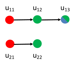
Figure 3: $u_{11}\rightleftharpoons_{\mathtt{CM}}u_{21}$ but $u_{11}\not\rightleftharpoons_{\mathtt{CMC}}u_{21}$.

where $\mathcal{V}^{-1}(u_{11})=\mathcal{V}^{-1}(u_{21})=\{r\},\mathcal{V}^{-1}(u_{12})=\mathcal{V}^{-1}(u_{22})=\{g\}$ and $\mathcal{V}^{-1}(u_{13})=\{b,g\}$ (see Remark 4 in Appendix 0.C).

Proposition 4

For all QdCMs $\mathcal{M}=(X,\stackrel{{\scriptstyle\rightarrow}}{{\mathcal{C}}},\mathcal{V})$ and $x_{1},x_{2}\in X$ the following holds: $x_{1}\,\rightleftharpoons_{\mathtt{CMC}}\,x_{2}$ implies $x_{1}\,\rightleftharpoons_{\mathtt{Tr}}\,x_{2}$.

The converse of Proposition 4 does not hold as shown in Figure 4 where $\mathcal{V}^{-1}(y_{11})=\mathcal{V}^{-1}(y_{12})=\mathcal{V}^{-1}(y_{21})=\mathcal{V}^{-1}(y_{22})=\mathcal{V}^{-1}(y_{24})=\{r\}\not=\{b\}=\mathcal{V}^{-1}(y_{13})=\mathcal{V}^{-1}(y_{23})$ and $y_{11}\rightleftharpoons_{\mathtt{Tr}}y_{21}$ but $y_{11}\not\rightleftharpoons_{\mathtt{CMC}}y_{21}$ (see Remark 5 in Appendix 0.C).

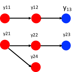
Figure 4: $y_{11}\rightleftharpoons_{\mathtt{Tr}}y_{21}$ but $y_{11}\not\rightleftharpoons_{\mathtt{CMC}}y_{21}$.

4.2 Logical Characterisation of CMC-bisimilarity for QdCMs

In order to provide a logical characterisation of CMC-bisimilarity, we extend IML with a “converse” of the modal operator of classical IML, thus exploiting the inverse of the binary relation underlying the QdCM. The result is a logic with the two modalities $\stackrel{{\scriptstyle\rightarrow}}{{\mathcal{N}}}$ and $\stackrel{{\scriptstyle\leftarrow}}{{\mathcal{N}}}$, with the expected meaning.

Definition 14 (Infinitary Modal Logic with Converse - IMLC)

For index set $I$ and $p\in{\tt AP}$ the abstract language of IMLC is defined as follows:

$$\Phi::=p\;|\;\neg\Phi\;|\;\bigwedge_{i\in I}\Phi_{i}\;|\;\stackrel{{\scriptstyle\rightarrow}}{{\mathcal{N}}}\Phi\;|\;\stackrel{{\scriptstyle\leftarrow}}{{\mathcal{N}}}\Phi.$$

The satisfaction relation for all QdCMs $\mathcal{M}$, points $x\in\mathcal{M}$, and IMLC formulas $\Phi$ is defined recursively on the structure of $\Phi$ as follows:

$$\begin{array}[]{r c l c l c l l}\mathcal{M},x&\models_{{\tt IMLC}}&p&\Leftrightarrow&x\in\mathcal{V}(p);\\ \mathcal{M},x&\models_{{\tt IMLC}}&\neg\,\Phi&\Leftrightarrow&\mathcal{M},x\models_{{\tt IMLC}}\Phi\mbox{ does not hold};\\ \mathcal{M},x&\models_{{\tt IMLC}}&\bigwedge_{i\in I}\Phi_{i}&\Leftrightarrow&\mathcal{M},x\models_{{\tt IMLC}}\Phi_{i}\mbox{ for all }i\in I;\\ \mathcal{M},x&\models_{{\tt IMLC}}&\stackrel{{\scriptstyle\rightarrow}}{{\mathcal{N}}}\Phi&\Leftrightarrow&x\in\stackrel{{\scriptstyle\rightarrow}}{{\mathcal{C}}}([\![\Phi]\!]^{\mathcal{M}});\\ \mathcal{M},x&\models_{{\tt IMLC}}&\stackrel{{\scriptstyle\leftarrow}}{{\mathcal{N}}}\Phi&\Leftrightarrow&x\in\stackrel{{\scriptstyle\leftarrow}}{{\mathcal{C}}}([\![\Phi]\!]^{\mathcal{M}}).\end{array}$$

$\bullet$

Definition 15 (IMLC-Equivalence)

Given QdCM $\mathcal{M}=(X,\stackrel{{\scriptstyle\rightarrow}}{{\mathcal{C}}},\mathcal{V})$, the equivalence relation $\simeq_{{\tt IMLC}}^{\mathcal{M}}\,\subseteq\,X\times X$ is defined as: $x_{1}\simeq_{{\tt IMLC}}^{\mathcal{M}}x_{2}$ if and only if for all IMLC formulas $\Phi$ the following holds: $\mathcal{M},x_{1}\models_{{\tt IMLC}}\Phi$ if and only if $\mathcal{M},x_{2}\models_{{\tt IMLC}}\Phi$. $\bullet$

In the sequel we will often abbreviate $\simeq_{{\tt IMLC}}^{\mathcal{M}}$ with $\simeq_{{\tt IMLC}}$.

Theorem 4.1

For all QdCMs $\mathcal{M}=(X,\stackrel{{\scriptstyle\rightarrow}}{{\mathcal{C}}},\mathcal{V})$, any CMC-Bisimulation $B$ over $X$ is included in the equivalence $\simeq_{{\tt IMLC}}^{\mathcal{M}}$.

The converse of Theorem 4.1 is given below.

Theorem 4.2

For all QdCMs $\mathcal{M}=(X,\stackrel{{\scriptstyle\rightarrow}}{{\mathcal{C}}},\mathcal{V})$, $\simeq_{{\tt IMLC}}^{\mathcal{M}}$ is a CMC-Bisimulation.

Corollary 2

For all QdCMs $\mathcal{M}=(X,\stackrel{{\scriptstyle\rightarrow}}{{\mathcal{C}}},\mathcal{V})$ we have that $\simeq_{{\tt IMLC}}^{\mathcal{M}}$ coincides with $\rightleftharpoons_{\mathtt{CMC}}^{\mathcal{M}}$. ∎

4.3 $\mathcal{C}$-bisimilarity for QdCMs

In this section, we recall a notion of bisimilarity for QdCMs that has been proposed in [14] and that is based on closure functions, instead of interior functions. We then prove that such a notion, which here we call $\mathcal{C}$-bisimilarity, coincides with CMC-bisimilarity. The introduction of $\mathcal{C}$-bisimilarity is motivated by the fact that we find it more intuitive, and its use makes several proofs simpler.

Definition 16 ($\mathcal{C}$-bisimilarity for QdCMs)

Given QdCM $\mathcal{M}=(X,\stackrel{{\scriptstyle\rightarrow}}{{\mathcal{C}}},\mathcal{V})$, a non empty relation $B\subseteq X\times X$ is a $\mathcal{C}$-bisimulation over $X$ if, whenever $(x_{1},x_{2})\in B$, the following holds:

1. $\mathcal{V}^{-1}{x_{1}}=\mathcal{V}^{-1}{x_{2}}$;

2. for all $x_{1}^{\prime}\in\stackrel{{\scriptstyle\rightarrow}}{{\mathcal{C}}}(\{x_{1}\})$ there exists $x_{2}^{\prime}\in\stackrel{{\scriptstyle\rightarrow}}{{\mathcal{C}}}(\{x_{2}\})$ such that $(x_{1}^{\prime},x_{2}^{\prime})\in B$;

3. for all $x_{2}^{\prime}\in\stackrel{{\scriptstyle\rightarrow}}{{\mathcal{C}}}(\{x_{2}\})$ there exists $x_{1}^{\prime}\in\stackrel{{\scriptstyle\rightarrow}}{{\mathcal{C}}}(\{x_{1}\})$ such that $(x_{1}^{\prime},x_{2}^{\prime})\in B$;

4. for all $x_{1}^{\prime}\in\stackrel{{\scriptstyle\leftarrow}}{{\mathcal{C}}}(\{x_{1}\})$ there exists $x_{2}^{\prime}\in\stackrel{{\scriptstyle\leftarrow}}{{\mathcal{C}}}(\{x_{2}\})$ such that $(x_{1}^{\prime},x_{2}^{\prime})\in B$;

5. for all $x_{2}^{\prime}\in\stackrel{{\scriptstyle\leftarrow}}{{\mathcal{C}}}(\{x_{2}\})$ there exists $x_{1}^{\prime}\in\stackrel{{\scriptstyle\leftarrow}}{{\mathcal{C}}}(\{x_{1}\})$ such that $(x_{1}^{\prime},x_{2}^{\prime})\in B$;

We say that $x_{1}$ and $x_{2}$ are $\mathcal{C}$-bisimilar, written $x_{1}\,\rightleftharpoons_{\mathcal{C}}^{\mathcal{M}}\,x_{2}$, if and only if there exists a $\mathcal{C}$-bisimulation $B$ such that $(x_{1},x_{2})\in B$. $\bullet$

As mentioned in Section 1, $\mathcal{C}$-bisimulation resembles (strong) Back and Forth bisimulation of [15], in particular for the presence of Conditions 4 and 5. Should we delete the above mentioned conditions, thus making our definition of $\mathcal{C}$-bisimulation more similar to classical strong bisimulation for transition systems, we would have to consider points $v_{12}$ and $v_{22}$ of Figure 5 bisimilar where $\mathcal{V}^{-1}(v_{11})=\{r\}\not=\{g\}=\mathcal{V}^{-1}(v_{21})$ and $\mathcal{V}^{-1}(v_{12})=\{b\}=\mathcal{V}^{-1}(v_{22})$.

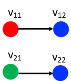
Figure 5: $v_{12}$ and $v_{22}$ are not $\mathcal{C}$-bisimilar.

We instead want to consider them as not being bisimilar because they are in the closure of (i.e. they are “near” to) points that are not bisimilar, namely $v_{11}$ and $v_{21}$. For instance, $v_{21}$ might represent a poisoned physical location (whereas $v_{11}$ is not poisoned) and so $v_{22}$ should not be considered equivalent to $v_{12}$ because the former can be reached from the poisoned location while the latter cannot.

4.4 $\mathcal{C}$-bisimilarity minimisation

In [14] we have shown a minimisation algorithm for $\rightleftharpoons_{\mathcal{C}}^{\mathcal{M}}$. The algorithm is defined in a coalgebraic setting: it takes an $\mathcal{F}$-coalgebra, for appropriate functor $\mathcal{F}$ in the category Set, and returns the bisimilarity quotient of its carrier set. The instantiation of the algorithm for (a coalgebraic interpretation of) QdCSs is implemented in the tool MiniLogicA, available for the major operating systems at https://github.com/vincenzoml/MiniLogicA.

4.5 Logical Characterisation of $\mathcal{C}$-bisimilarity

In this section we present ISLCS, an infinitary version of a variant of the Spatial Logic for Closure Spaces (SLCS). SLCS has been proposed in [12] and its basic modal operators are near ($\mathcal{N}$), surrounded ($\mathcal{S}$) and propagation ($\mathcal{P}$), whereas reachability operators are derived from the above. The variant of SLCS that we use in this section, instead, has only two basic reachability operators $\stackrel{{\scriptstyle\rightarrow}}{{\rho}}$ and $\stackrel{{\scriptstyle\leftarrow}}{{\rho}}$, as in [14]. We will show that, when the underlying interptretation model is quasi-discrete, $\mathcal{N}$ can be derived from the reachability operators: more precisely, $\stackrel{{\scriptstyle\rightarrow}}{{\mathcal{N}}}$ can be derived from $\stackrel{{\scriptstyle\leftarrow}}{{\rho}}$ and $\stackrel{{\scriptstyle\leftarrow}}{{\mathcal{N}}}$ from $\stackrel{{\scriptstyle\rightarrow}}{{\rho}}$ (Lemma 1 below). Furthermore, we show that ISLCS characterises $\mathcal{C}$-bisimilarity. We also prove that an appropirate sub-logic of ISLCS is sufficient for characterising $\mathcal{C}$-bisimilarity and that such sub-logic coincides with IMLC. As a side-result, we get the coincidence of CMC-bisimilarity and $\mathcal{C}$-bisimilarity.

Definition 17 (Infinitary SLCS - ISLCS)

For index set $I$ and $p\in{\tt AP}$ the abstract language of ISLCS is defined as follows:

$$\Phi::=p\;|\;\neg\Phi\;|\;\bigwedge_{i\in I}\Phi_{i}\;|\;\stackrel{{\scriptstyle\rightarrow}}{{\rho}}\Phi_{1}[\Phi_{2}]\;|\;\stackrel{{\scriptstyle\leftarrow}}{{\rho}}\Phi_{1}[\Phi_{2}].$$

The satisfaction relation for QdCMs $\mathcal{M}$, $x\in\mathcal{M}$, and ISLCS formulas $\Phi$ is defined recursively on the structure of $\Phi$ as follows:

$$\begin{array}[]{r c l c l c l}\mathcal{M},x&\models_{{\tt ISLCS}}&p&\Leftrightarrow&x\in\mathcal{V}(p)\\ \mathcal{M},x&\models_{{\tt ISLCS}}&\neg\,\Phi&\Leftrightarrow&\mathcal{M},x\models_{{\tt ISLCS}}\Phi\mbox{ does not hold}\\ \mathcal{M},x&\models_{{\tt ISLCS}}&\bigwedge_{i\in I}\Phi_{i}&\Leftrightarrow&\mathcal{M},x\models_{{\tt ISLCS}}\Phi_{i}\mbox{ for all }i\in I\\ \mathcal{M},x&\models_{{\tt ISLCS}}&\stackrel{{\scriptstyle\rightarrow}}{{\rho}}\Phi_{1}[\Phi_{2}]&\Leftrightarrow&\mbox{there exist path }\pi\mbox{ and index }\ell\mbox{ such that }\\ &&&&\mbox{\hskip 7.22743pt}\pi(0)=x\mbox{ and }\\ &&&&\mbox{\hskip 7.22743pt}\pi(\ell)\models_{{\tt ISLCS}}\Phi_{1}\mbox{ and }\\ &&&&\mbox{\hskip 7.22743pt}\mbox{for all }j\mbox{ such that }0<j<\ell\mbox{ the following holds:}\\ &&&&\mbox{\hskip 14.45377pt}\pi(j)\models_{{\tt ISLCS}}\Phi_{2};\\ \mathcal{M},x&\models_{{\tt ISLCS}}&\stackrel{{\scriptstyle\leftarrow}}{{\rho}}\Phi_{1}[\Phi_{2}]&\Leftrightarrow&\mbox{there exist path }\pi\mbox{ and index }\ell\mbox{ such that }\\ &&&&\mbox{\hskip 7.22743pt}\pi(\ell)=x\mbox{ and }\\ &&&&\mbox{\hskip 7.22743pt}\pi(0)\models_{{\tt ISLCS}}\Phi_{1}\mbox{ and }\\ &&&&\mbox{\hskip 7.22743pt}\mbox{for all }j\mbox{ such that }0<j<\ell\mbox{ the following holds:}\\ &&&&\mbox{\hskip 14.45377pt}\pi(j)\models_{{\tt ISLCS}}\Phi_{2}.\end{array}$$

$\bullet$

Definition 18 (ISLCS-Equivalence)

Given QdCM $\mathcal{M}=(X,\stackrel{{\scriptstyle\rightarrow}}{{\mathcal{C}}},\mathcal{V})$, the equivalence relation $\simeq_{{\tt ISLCS}}^{\mathcal{M}}\,\subseteq\,X\times X$ is defined as: $x_{1}\simeq_{{\tt ISLCS}}^{\mathcal{M}}x_{2}$ if and only if for all ISLCS formulas $\Phi$ the following holds: $\mathcal{M},x_{1}\models_{{\tt ISLCS}}\Phi$ if and only if $\mathcal{M},x_{2}\models_{{\tt ISLCS}}\Phi$. $\bullet$

Theorem 4.3

For all QdCMs $\mathcal{M}=(X,\stackrel{{\scriptstyle\rightarrow}}{{\mathcal{C}}},\mathcal{V})$, any $\mathcal{C}$-Bisimulation $B$ over $X$ is included in the equivalence $\simeq_{{\tt ISLCS}}^{\mathcal{M}}$.

The converse of Theorem 4.3 is given below.

Theorem 4.4

For all QdCMs $\mathcal{M}=(X,\stackrel{{\scriptstyle\rightarrow}}{{\mathcal{C}}},\mathcal{V})$, $\simeq_{{\tt ISLCS}}^{\mathcal{M}}$ is a $\mathcal{C}$-Bisimulation.

Corollary 3

For all QdCMs $\mathcal{M}=(X,\stackrel{{\scriptstyle\rightarrow}}{{\mathcal{C}}},\mathcal{V})$ we have that $\simeq_{{\tt ISLCS}}^{\mathcal{M}}$ coincides with $\rightleftharpoons_{\mathcal{C}}^{\mathcal{M}}$. ∎

Let $\stackrel{{\scriptstyle\rightarrow}}{{\mathcal{N}}}$ and $\stackrel{{\scriptstyle\leftarrow}}{{\mathcal{N}}}$ be defined as in Definition 14.

Lemma 1

For all QdCMs $\mathcal{M}=(X,\stackrel{{\scriptstyle\rightarrow}}{{\mathcal{C}}},\mathcal{V})$, the following holds:
$\stackrel{{\scriptstyle\rightarrow}}{{\mathcal{N}}}\Phi\equiv\stackrel{{\scriptstyle\leftarrow}}{{\rho}}\Phi[{\tt false}]$ and $\stackrel{{\scriptstyle\leftarrow}}{{\mathcal{N}}}\Phi\equiv\stackrel{{\scriptstyle\rightarrow}}{{\rho}}\Phi[{\tt false}]$.

Theorem 4.5

For all QdCMs $\mathcal{M}=(X,\stackrel{{\scriptstyle\rightarrow}}{{\mathcal{C}}},\mathcal{V})$, $\simeq_{{\tt IMLC}}^{\mathcal{M}}$ coincides with $\rightleftharpoons_{\mathcal{C}}^{\mathcal{M}}$.

From Corollary 2 and Theorem 4.5 we get the following

Corollary 4

For all QdCMs $\mathcal{M}=(X,\stackrel{{\scriptstyle\rightarrow}}{{\mathcal{C}}},\mathcal{V})$ we have that $\rightleftharpoons_{\mathtt{CMC}}^{\mathcal{M}}$ coincides with $\rightleftharpoons_{\mathcal{C}}^{\mathcal{M}}$. ∎

5 Path-bisimilarity

CM-bisimilarity, and its refinements CMC-bisimilarity and $\mathcal{C}$-bisimilarity, are a fundamental starting point for the study of bisimulations in space due to their strong links to Topo-bisimulation. On the other hand, they are somehow too much fine grain relations for reasoning about general properties of space and related notions of model minimisation. For instance, with reference to the model of Figure 6, where all red points satisfy only atomic proposition $r$ while the blue ones satisfy only $b$, the point at the center of the left part of the model is not CMC-bisimilar to any other red point in the model. This is because CMC-bisimilarity is based on the fact that points reachable “in one step” are taken into consideration, as it is clear from the equivalent $\mathcal{C}$-bisimilarity definition. This, in turn, gives bisimilarity a sort of “counting” power, that goes against the idea that, for instance, the left part of the model could be represented by the right part—and that, actually, both parts could be represented by a minimal model consisting of just one red point and one blue point, connected by a symmetric arrow, which would convey an idea of space scaling. Such scaling would be quite useful when dealing, for instance, with models representing images—as briefly mentioned in Section 1. Such models are QdCMs where the “points” are pixels or voxels and the underlying relation is the so called Adjacency relation, i.e. a reflexive and symmetric relation such that each pixel/voxel is related to all the pixel/voxel that share an edge or a vertex with it. In this and in the next sections, we present weaker notions of bisimilarity, namely Path-bisimilarity and CoPa-bisimilarity, with the aim of capturing the intuitive notions briefly discussed above. We start with the definition of Path-bisimilarity.

                

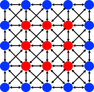
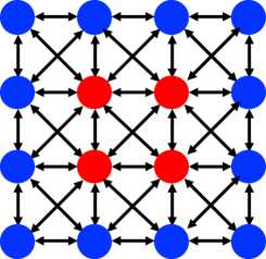
Figure 6: A model consisting of two parts

5.1 Path-bisimilarity

Definition 19 (Path-bisimilarity)

Given CM $\mathcal{M}=(X,\mathcal{C},\mathcal{V})$ and index space $\mathcal{J}=(I,\mathcal{C}^{\mathcal{J}})$, a non empty relation $B\subseteq X\times X$ is a Path-bisimulation over $X$ if, whenever $(x_{1},x_{2})\in B$, the following holds:

1. $\mathcal{V}^{-1}(x_{1})=\mathcal{V}^{-1}(x_{2})$;

2. for all $\pi_{1}\in\mathtt{BPaths^{F}}_{\mathcal{J},\mathcal{M}}(x_{1})$, there exists $\pi_{2}\in\mathtt{BPaths^{F}}_{\mathcal{J},\mathcal{M}}(x_{2})$ such that
   $(\pi_{1}(\mathtt{len}(\pi_{1})),\pi_{2}(\mathtt{len}(\pi_{2})))\in B$;

3. for all $\pi_{2}\in\mathtt{BPaths^{F}}_{\mathcal{J},\mathcal{M}}(x_{2})$, there exists $\pi_{1}\in\mathtt{BPaths^{F}}_{\mathcal{J},\mathcal{M}}(x_{1})$ such that
   $(\pi_{1}(\mathtt{len}(\pi_{1})),\pi_{2}(\mathtt{len}(\pi_{2})))\in B$;

4. for all $\pi_{1}\in\mathtt{BPaths^{T}}_{\mathcal{J},\mathcal{M}}(x_{1})$, there exists $\pi_{2}\in\mathtt{BPaths^{T}}_{\mathcal{J},\mathcal{M}}(x_{2})$ such that.
   $(\pi_{1}(0),\pi_{2}(0))\in B$;

5. for all $\pi_{2}\in\mathtt{BPaths^{T}}_{\mathcal{J},\mathcal{M}}(x_{2})$, there exists $\pi_{1}\in\mathtt{BPaths^{T}}_{\mathcal{J},\mathcal{M}}(x_{1})$ such that
   $(\pi_{1}(0),\pi_{2}(0))\in B$.

$x_{1}$ and $x_{2}$ are Path-bisimilar, written $x_{1}\,\rightleftharpoons_{\mathtt{Pth}}^{\mathcal{M}}\,x_{2}$, if and only if there is a Path-bisimulation $B$ over $X$ such that $(x_{1},x_{2})\in B$. $\bullet$

In the sequel, we will say that two points are AP-equivalent, written $\rightleftharpoons_{{\tt AP}}$, if they satisfy exactly the same atomic propositions. In other words: $\rightleftharpoons_{{\tt AP}}$ is the set $\{(x_{1},x_{2})\,|\,\mathcal{V}^{-1}(x_{1})=\mathcal{V}^{-1}(x_{2})\}$. The following proposition trivially follows from the relevant definitions:

Proposition 5

For all CMs $\mathcal{M}=(X,\mathcal{C},\mathcal{V})$ and $x_{1},x_{2}\in X$ the following holds:
$x_{1}\,\rightleftharpoons_{\mathtt{Pth}}\,x_{2}$ implies $x_{1}\,\rightleftharpoons_{{\tt AP}}\,x_{2}$.∎

The converse of Proposition 5 does not hold, as shown again in Figure 4 where we leave to the reader the easy task of checking that $y_{11}\not\rightleftharpoons_{\mathtt{Pth}}y_{21}$ despite $y_{11}\rightleftharpoons_{{\tt AP}}y_{21}$ since $\mathcal{V}^{-1}(y_{11})=\mathcal{V}^{-1}(y_{21})=\{r\}$.

In Figure 7 (left) an image representing a maze is shown; green pixels are the exit ones wheras the blue ones represent possible starting points; walls are represented by black pixels. In Figure 7 (right) the minimal model via Path-bisimilarity is shown; it actually coincides with the one we would have obtained using $\rightleftharpoons_{{\tt AP}}$ instead. In practical terms, some important features of the image of the maze are lost in its Path-bisimilarity minimisation, such as the fact that some starting points cannot reach the exit, unless passing through walls, which should not happen! This is due to the fact that Path-bisimilarity abstracts from the structure of the underlying paths. In Section 6 we will address this issue explicitly and refine Path-bisimilarity into a stronger one, namely CoPa-bisimilarity.

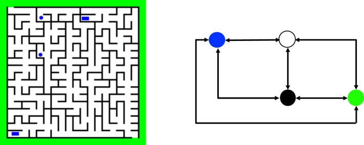
Figure 7: A maze and its reduced model modulo Path-bisimilarity.

Proposition 6

For all QdCMs $\mathcal{M}=(X,\mathcal{C},\mathcal{V})$ and $x_{1},x_{2}\in X$ the following holds: $x_{1}\,\rightleftharpoons_{\mathtt{CMC}}\,x_{2}$ implies $x_{1}\,\rightleftharpoons_{\mathtt{Pth}}\,x_{2}$.

The converse of Proposition 6 does not hold, as shown in Figure 8

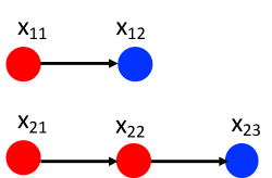
Figure 8: $x_{11}\rightleftharpoons_{\mathtt{Pth}}x_{21}$ but $x_{11}\not\rightleftharpoons_{\mathtt{CMC}}x_{21}$.

where $\mathcal{V}^{-1}(x_{11})=\mathcal{V}^{-1}(x_{21})=\mathcal{V}^{-1}(x_{22})=\{r\}\not=\{b\}=\mathcal{V}^{-1}(x_{12})=\mathcal{V}^{-1}(x_{23})$ and $x_{11}\rightleftharpoons_{\mathtt{Pth}}x_{21}$ but $x_{11}\not\rightleftharpoons_{\mathtt{CMC}}x_{21}$ (see Remark 6 of Appendix 0.D).

Remark 2

It is worth pointing out that the analogous of Proposition 6 for general CMs does not hold. In fact there are models with points that are CM-bisimilar but not Path-bisimilar, as shown in Figure 9 where an Euclidean model $\mathcal{M}=(X,\mathcal{C},\mathcal{V})$ is shown such that $X=(-\infty,0)\cup(0,\infty)$, $\mathcal{C}$ is the standard closure operator for the real line $\mathbb{R}$, $A,B$ and $C$ are non-empty intervals with $B\subset A\subset(-\infty,0)$, and $C\subset(0,+\infty)$, $\mathcal{V}(g)=A\cup C$ and $\mathcal{V}(r)=\{k\}$, with $k\in A\setminus B$. In such a model, $x_{1}\rightleftharpoons_{\mathtt{CM}}x_{2}$ for all $(x_{1},x_{2})\in B\times C$. In fact $B\times C$ is a CM-bisimulation, as shown in the sequel. Take any $(x_{1},x_{2})\in B\times C$; clearly $\mathcal{V}^{-1}(x_{1})=\mathcal{V}^{-1}(x_{2})$ by construction; let $S_{1}\subseteq(-\infty,0)$ be any set such that $x_{1}\in\mathcal{I}(S_{1})$; then, for what concerns Condition 2 of Definition 10, take $S_{2}=C=\mathcal{I}(C)$; for each $s_{2}\in S_{2}$ there is $s_{1}\in S_{1}\cap B$ such that $(s_{1},s_{2})\in B\times C$, by definition of $B\times C$; let finally $S_{2}\subseteq(0,+\infty)$ be any set such that $x_{2}\in\mathcal{I}(S_{2})$ then, for what concerns Condition 3 of Definition 10, take $S_{1}=B=\mathcal{I}(B)$: for each $s_{1}\in S_{1}$ there is $s_{2}\in S_{2}\cap C$ such that $(s_{1},s_{2})\in B\times C$, by definition of $B\times C$. On the other hand, $x_{1}\not\rightleftharpoons_{\mathtt{Pth}}x_{2}$, since there cannot be any Path-bisimulation for $x_{1}$ and $x_{2}$ as above. This is because $x_{1}\in A$, since $B\subset A$, and $x_{1}\stackrel{{\scriptstyle}}{{\Longrightarrow}}k$ with $r\in\mathcal{V}^{-1}(k)$ whereas $r\not\in\mathcal{V}^{-1}(x)$ for all $x\in(0,+\infty)$.

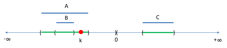
Figure 9: For all $x_{1}$ and $x_{2}$ such that $(x_{1},x_{2})\in B\times C$ we have $x_{1}\rightleftharpoons_{\mathtt{CM}}x_{2}$ but $x_{1}\not\rightleftharpoons_{\mathtt{Pth}}x_{2}$.

Downstream of Remark 2 we can strengthen Definition 10 so that we get an adaptation for CMs of the notion of INL-bisimilarity proposed in [6] for general neighbourhood models:

Definition 20 (INL-bisimilarity for CMs)

Given CM $\mathcal{M}=(X,\mathcal{C},\mathcal{V})$, a non empty relation $B\subseteq X\times X$ is a INL-bisimulation over $X$ if, whenever $(x_{1},x_{2})\in B$, the following holds:

1. $\mathcal{V}^{-1}(x_{1})=\mathcal{V}^{-1}(x_{2})$;

2. for all neighbourhoods $S_{1}$ of $x_{1}$ there is a neighbourhood $S_{2}$ of $x_{2}$ such that:

   1. for all $s_{2}\in S_{2}$, there is $s_{1}\in S_{1}$ with $(s_{1},s_{2})\in B$;

   2. for all $s_{1}\in S_{1}$, there is $s_{2}\in S_{2}$ with $(s_{1},s_{2})\in B$;

3. for all neighbourhoods $S_{2}$ of $x_{2}$ there is a neighbourhood $S_{1}$ of $x_{1}$ such that:

   1. for all $s_{1}\in S_{1}$, there is $s_{2}\in S_{2}$ with $(s_{1},s_{2})\in B$;

   2. for all $s_{2}\in S_{2}$, there is $s_{1}\in S_{1}$ with $(s_{1},s_{2})\in B$.

$x_{1}$ and $x_{2}$ are INL-bisimilar, written $x_{1}\,\rightleftharpoons_{\mathtt{{\tt INL}}}^{\mathcal{M}}\,x_{2}$, if and only if there is a INL-bisimulation $B$ over $X$ such that $(x_{1},x_{2})\in B$. $\bullet$

We can now prove the following

Proposition 7

For all path-connected CMs $\mathcal{M}=(X,\mathcal{C},\mathcal{V})$ and $x_{1},x_{2}\in X$ the following holds: $x_{1}\rightleftharpoons_{\mathtt{{\tt INL}}}x_{2}$ implies $x_{1}\rightleftharpoons_{\mathtt{Pth}}x_{2}$.

The following proposition shows that $\rightleftharpoons_{\mathtt{Pth}}$ and $\rightleftharpoons_{\mathtt{Tr}}$ uncomparable:

Proposition 8

There exist CMs $\mathcal{M}$ and points $x_{1},x_{2}\in\mathcal{M}$ such that $x_{1}\rightleftharpoons_{\mathtt{Pth}}x_{2}$ and $x_{1}\not\rightleftharpoons_{\mathtt{Tr}}x_{2}$; similarly, there are CMs $\mathcal{M}$ and points $x_{1},x_{2}\in\mathcal{M}$ such that $x_{1}\not\rightleftharpoons_{\mathtt{Pth}}x_{2}$ and $x_{1}\rightleftharpoons_{\mathtt{Tr}}x_{2}$.

As an example of the first case, let us consider again the model of Figure 8: we have already seen that $x_{11}\rightleftharpoons_{\mathtt{Pth}}x_{21}$; but $x_{11}\not\rightleftharpoons_{\mathtt{Tr}}x_{21}$ since $\{r\}\!\!\cdot\!\!\{b\}^{\omega}\in\mathtt{Tr}(\mathtt{BPaths^{F}}(x_{11}))\setminus\mathtt{Tr}(\mathtt{BPaths^{F}}(x_{21}))$. As for the second case, let us consider again the model of Figure 4: we have already seen that $y_{11}\rightleftharpoons_{\mathtt{Tr}}y_{21}$ and that $y_{11}\not\rightleftharpoons_{\mathtt{Pth}}y_{21}$.

5.2 Logical Characterisation of Path-bisimilarity

In this section we show that a sub-logic of ISLCS fully characterises Path-bisimilarity. We first define the Infinitary Reachability Logic, IRL for short and show that IRL is a sub-logic of ISLCS obtained by forcing the second argument of $\stackrel{{\scriptstyle\rightarrow}}{{\rho}}$ and $\stackrel{{\scriptstyle\leftarrow}}{{\rho}}$ to ${\tt true}$. Then we provide the characterisation result.

Definition 21 (Infinitary Reachability Logic - IRL)

For index set $I$ and $p\in{\tt AP}$ the abstract language of IRL is defined as follows:

$$\Phi::=p\;|\;\neg\Phi\;|\;\bigwedge_{i\in I}\Phi_{i}\;|\;\stackrel{{\scriptstyle\rightarrow}}{{\sigma}}\Phi\;|\;\stackrel{{\scriptstyle\leftarrow}}{{\sigma}}\Phi.$$

The satisfaction relation for all CMs $\mathcal{M}$, $x\in\mathcal{M}$, and IRL formulas $\Phi$ is defined recursively on the structure of $\Phi$ as follows:

$$\begin{array}[]{r c l c l c l l}\mathcal{M},x&\models_{{\tt IRL}}&p&\Leftrightarrow&x\in\mathcal{V}(p);\\ \mathcal{M},x&\models_{{\tt IRL}}&\neg\,\Phi&\Leftrightarrow&\mathcal{M},x\models_{{\tt IRL}}\Phi\mbox{ does not hold};\\ \mathcal{M},x&\models_{{\tt IRL}}&\bigwedge_{i\in I}\Phi_{i}&\Leftrightarrow&\mathcal{M},x\models_{{\tt IRL}}\Phi_{i}\mbox{ for all }i\in I;\\ \mathcal{M},x&\models_{{\tt IRL}}&\stackrel{{\scriptstyle\rightarrow}}{{\sigma}}\Phi&\Leftrightarrow&\mbox{there exist path }\pi\mbox{ and index }\ell\mbox{ such that }\\ &&&&\mbox{\hskip 7.22743pt}\pi(0)=x\mbox{ and }\pi(\ell)\models_{{\tt IRL}}\Phi;\\ \mathcal{M},x&\models_{{\tt IRL}}&\stackrel{{\scriptstyle\leftarrow}}{{\sigma}}\Phi&\Leftrightarrow&\mbox{there exist path }\pi\mbox{ and index }\ell\mbox{ such that }\\ &&&&\mbox{\hskip 7.22743pt}\pi(\ell)=x\mbox{ and }\pi(0)\models_{{\tt IRL}}\Phi.\\ \end{array}$$

$\bullet$

The following proposition trivially follows from the relevant definitions:

Proposition 9

For all CMs $\mathcal{M}=(X,\mathcal{C},\mathcal{V})$ and $x_{1},x_{2}\in X$ the following holds:
$\stackrel{{\scriptstyle\rightarrow}}{{\sigma}}\Phi\equiv\stackrel{{\scriptstyle\rightarrow}}{{\rho}}\Phi[{\tt true}]$ and $\stackrel{{\scriptstyle\leftarrow}}{{\sigma}}\Phi\equiv\stackrel{{\scriptstyle\leftarrow}}{{\rho}}\Phi[{\tt true}]$.∎

Definition 22 (IRL-Equivalence)

Given CM $\mathcal{M}=(X,\mathcal{C},\mathcal{V})$, the equivalence relation $\simeq_{{\tt IRL}}^{\mathcal{M}}\,\subseteq\,X\times X$ is defined as: $x_{1}\simeq_{{\tt IRL}}^{\mathcal{M}}x_{2}$ if and only if for all IRL formulas $\Phi$ the following holds: $\mathcal{M},x_{1}\models_{{\tt IRL}}\Phi$ if and only if $\mathcal{M},x_{2}\models_{{\tt IRL}}\Phi$. $\bullet$

Theorem 5.1

For all CMs $\mathcal{M}=(X,\mathcal{C},\mathcal{V})$, any Path-Bisimulation $B$ over $X$ is included in the equivalence $\simeq_{{\tt IRL}}^{\mathcal{M}}$.

The converse of Theorem 5.1 is given below.

Theorem 5.2

For all CMs $\mathcal{M}=(X,\mathcal{C},\mathcal{V})$, $\simeq_{{\tt IRL}}^{\mathcal{M}}$ is a Path-bisimulation.

Corollary 5

For all CMs $\mathcal{M}=(X,\mathcal{C},\mathcal{V})$ we have that $\simeq_{{\tt IRL}}^{\mathcal{M}}$ coincides with $\rightleftharpoons_{\mathtt{Pth}}^{\mathcal{M}}$. ∎

6 CoPa-bisimilarity

Path-bisimilarity is in some sense too weak, too abstract; nothing whatsoever is required of the relevant paths, except their starting points being fixed and related by the bisimulation, and their end-points be in the bisimulation as well. A deeper insight into the structure of such paths would be desirable as well as some, relatively high level, requirements over them. To that purpose we resort to a notion of “compatibility” between relevant paths that essentially requires each of them to be composed of a non-empty sequence of non-empty, adjacent “zones”. More precisely, both paths under consideration in a transfer condition should share the same structure, as follows (see Figure 10):

• both paths are composed by a sequence of (non-empty) “zones”;

• the number of zones should be the same in both paths, but

• the length of “corresponding” zones can be different, as well as the length of the two paths;

• each point in one zone of a path should be related by the bisimulation to every point in the corresponding zone of the other path.

This notion of compatibility gives rise to Compatible Path bisimulation, CoPa-bisimulation, defined below. We note that the notion of CoPa-bisimulation turns out to be reminiscent of that of Equivalence with respect to Stuttering for transition systems proposed in [7], although in a totally different context and with a quite different definition: the latter is defined via a convergent sequence of relations and makes use of a different notion of path than the one of CS used in this paper. Finally, [7] is focussed on CTL/CTL^∗, which implies a flow of time with single past (i.e. trees), which is not the case for structures representing space.

Figure 10: Zones in relevant paths.

6.1 CoPa-bisimilarity

Definition 23 (CoPa-bisimilarity)

Given CM $\mathcal{M}=(X,\mathcal{C},\mathcal{V})$ and index space $\mathcal{J}=(I,\mathcal{C}^{\mathcal{J}})$, a non empty relation $B\subseteq X\times X$ is a CoPa-bisimulation over $X$ if, whenever $(x_{1},x_{2})\in B$, the following holds:

1. $\mathcal{V}^{-1}(x_{1})=\mathcal{V}^{-1}(x_{2})$;

2. for all $\pi_{1}\in\mathtt{BPaths^{F}}_{\mathcal{J},\mathcal{M}}(x_{1})$ such that
   $(\pi_{1}(i_{1}),x_{2})\in B$ for all $i_{1}\in\{\iota\,|\,0\leq\iota<\mathtt{len}(\pi_{1})\}$,
   there is $\pi_{2}\in\mathtt{BPaths^{F}}_{\mathcal{J},\mathcal{M}}(x_{2})$ such that the following holds:
   $(x_{1},\pi_{2}(i_{2}))\in B$ for all $i_{2}\in\{\iota\,|\,0\leq\iota<\mathtt{len}(\pi_{2})\}$, and
   $(\pi_{1}(\mathtt{len}(\pi_{1})),\pi_{2}(\mathtt{len}(\pi_{2})))\in B$;

3. for all $\pi_{2}\in\mathtt{BPaths^{F}}_{\mathcal{J},\mathcal{M}}(x_{2})$ such that
   $(x_{1},\pi_{2}(i_{2}))\in B$ for all $i_{2}\in\{\iota\,|\,0\leq\iota<\mathtt{len}(\pi_{2})\}$,
   there is $\pi_{1}\in\mathtt{BPaths^{F}}_{\mathcal{J},\mathcal{M}}(x_{1})$ such that the following holds:
   $(\pi_{1}(i_{1}),x_{2})\in B$ for all $i_{1}\in\{\iota\,|\,0\leq\iota<\mathtt{len}(\pi_{1})\}$, and
   $(\pi_{1}(\mathtt{len}(\pi_{1})),\pi_{2}(\mathtt{len}(\pi_{2})))\in B$;

4. for all $\pi_{1}\in\mathtt{BPaths^{T}}_{\mathcal{J},\mathcal{M}}(x_{1})$ such that
   $(\pi_{1}(i_{1}),x_{2})\in B$ for all $i_{1}\in\{\iota\,|\,0<\iota\leq\mathtt{len}(\pi_{1})\}$,
   there is $\pi_{2}\in\mathtt{BPaths^{T}}_{\mathcal{J},\mathcal{M}}(x_{2})$ such that the following holds:
   $(x_{1},\pi_{2}(i_{2}))\in B$ for all $i_{2}\in\{\iota\,|\,0<\iota\leq\mathtt{len}(\pi_{2})\}$, and
   $(\pi_{1}(0),\pi_{2}(0))\in B$;

5. for all $\pi_{2}\in\mathtt{BPaths^{T}}_{\mathcal{J},\mathcal{M}}(x_{2})$ such that
   $(x_{1},\pi_{2}(i_{2}))\in B$ for all $i_{2}\in\{\iota\,|\,0<\iota\leq\mathtt{len}(\pi_{2})\}$,
   there is $\pi_{1}\in\mathtt{BPaths^{T}}_{\mathcal{J},\mathcal{M}}(x_{1})$ such that the following holds:
   $(\pi_{1}(i_{1}),x_{2})\in B$ for all $i_{1}\in\{\iota\,|\,0<\iota\leq\mathtt{len}(\pi_{1})\}$, and
   $(\pi_{1}(0),\pi_{2}(0))\in B$;

$x_{1}$ and $x_{2}$ are CoPa-bisimilar, written $x_{1}\,\rightleftharpoons_{\mathtt{CoPa}}^{\mathcal{M}}\,x_{2}$, if there is a CoPa-bisimulation $B$ over $X$ such that $(x_{1},x_{2})\in B$. $\bullet$

Figure 11 shows the minimal model modulo CoPa-bisimilarity of the maze image shown in Figure 7. It is easy to see that this reduced model retains more information than that of Figure 7 (right). In particular, in this model three different representatives of white points are present:

• one that is directly connected both with a representative of a blue starting point and with a representative of a green exit point; this represents the situation in which from a blue starting point the exit can be reached walking through the maze (i.e. white points);

• one that is directly connected with a representative of a green point, but it is not directly connected with a representative of a blue point; this represents parts of the maze from which an exit could be reached, but that are separated (by walls) from areas where there are starting points (see below), and

• one that is directly connected to a representative of a blue starting point but that is not directly connected to a green exit point—that can be reached only by passing through the black point; this represents the fact that the relevant blue starting point cannot reach the exit because it will always be blocked by a wall.

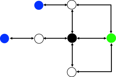
Figure 11: Reduced model of the maze of Fig. 8 (left), modulo CoPa-bisimilarity.

The following proposition can be easily proved from the relevant definitions:

Proposition 10

For all CMs $\mathcal{M}=(X,\mathcal{C},\mathcal{V})$ and $x_{1},x_{2}\in X$ the following holds: $x_{1}\,\rightleftharpoons_{\mathtt{CoPa}}\,x_{2}$ implies $x_{1}\,\rightleftharpoons_{\mathtt{Pth}}\,x_{2}$.∎

The converse of Proposition 10 does not hold, as shown in Figure 12. Relation $B=\{(t_{11},t_{21}),(t_{12},t_{22}),(t_{13},t_{23}),(t_{14},t_{24}),(t_{15},t_{25})\}$ is a Path-bisimulation, so $t_{11}\rightleftharpoons_{\mathtt{Pth}}t_{21}$. On the other hand, Condition 2 of Definition 23 cannot be fulfilled for any $\pi_{1}\in\mathtt{BPaths^{F}}(t_{11})$ such that $\pi_{1}(j)=t_{13}$ for some $j>0$ since for every $\pi_{2}\in\mathtt{BPaths^{F}}(t_{21})$ there is $k$ such that $g\in\mathcal{V}^{-1}(\pi_{2}(k))$, wheras $g\not\in\mathcal{V}^{-1}(\pi_{1}(h))$ for all $h$.

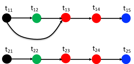
Figure 12: $t_{11}\rightleftharpoons_{\mathtt{Pth}}t_{21}$ but $t_{11}\not\rightleftharpoons_{\mathtt{CoPa}}t_{21}$.

Proposition 11

For all QdCMs $\mathcal{M}=(X,\stackrel{{\scriptstyle\rightarrow}}{{\mathcal{C}}},\mathcal{V})$ and $x_{1},x_{2}\in X$ the following holds: $x_{1}\,\rightleftharpoons_{\mathtt{CMC}}\,x_{2}$ implies $x_{1}\,\rightleftharpoons_{\mathtt{CoPa}}\,x_{2}$.

The converse of Proposition 11 does not hold; again with reference to Figure 8, it is easy to see that $B=\{(x_{11},x_{21}),(x_{11},x_{22}),(x_{12},x_{23})\}$ is a CoPa-bisimulation, and so $x_{11}\rightleftharpoons_{\mathtt{CoPa}}x_{21}$. On the other hand, as we have already seen, $x_{11}\not\rightleftharpoons_{\mathtt{CMC}}x_{21}$.

The following proposition shows that $\rightleftharpoons_{\mathtt{CoPa}}$ and $\rightleftharpoons_{\mathtt{Tr}}$ are uncomparable.

Proposition 12

There exist CMs $\mathcal{M}$ and points $x_{1},x_{2}\in\mathcal{M}$ such that $x_{1}\rightleftharpoons_{\mathtt{CoPa}}x_{2}$ and $x_{1}\not\rightleftharpoons_{\mathtt{Tr}}x_{2}$; similarly, there are CMs $\mathcal{M}$ and points $x_{1},x_{2}\in\mathcal{M}$ such that $x_{1}\not\rightleftharpoons_{\mathtt{CoPa}}x_{2}$ and $x_{1}\rightleftharpoons_{\mathtt{Tr}}x_{2}$.

As an example of the first case, let us consider again the model of Figure 8: we have already seen that $x_{11}\rightleftharpoons_{\mathtt{CoPa}}x_{21}$ and that $x_{11}\not\rightleftharpoons_{\mathtt{Tr}}x_{21}$. As for the second case, let us consider again the model of Figure 4: we have already seen that $x_{11}\not\rightleftharpoons_{\mathtt{Pth}}x_{21}$, and thus, by Proposition 10 we get $x_{11}\not\rightleftharpoons_{\mathtt{CoPa}}x_{21}$; but we have already seen that $x_{11}\rightleftharpoons_{\mathtt{Tr}}x_{21}$.

6.2 CoPa-bisimilarity minimisation

In this section we show how CoPa-bisimilarity minimisation can be achieved using results from [17] on minimisation of Divergence-blind Stuttering Equivalence. We first recall the definition of Divergence-blind Stuttering Equivalence (Def. 2.2 of [17]):

Definition 24

Divergence-blind Stuttering Equivalence (dbs-Eq).
Let $K=(S,{\tt AP}{},R,L)$ be a Kripke structure. A symmetric relation $E\subseteq S\times S$ is a divergence-blind stuttering equivalence if and only if for all $s,t\in S$ such that $s\,E\,t$:

1. $L(s)=L(t)$, and

2. for all $s^{\prime}\in S$, if $s\,R\,s^{\prime}$ then there are $t_{0},\ldots,t_{k}\in S$ for some $k\in\mathbb{N}$ such that $t=t_{0},s\,E\,t_{i},t_{i}\,R\,t_{i+1}$ for all $i<k$, and $s^{\prime}\,E\,t_{k}$.

We say that two states $s,t\in S$ are divergence-blind stuttering equivalent, notation $s\rightleftharpoons_{\mathtt{dbs}}t$, if and only if there is a divergence-blind stuttering equivalence relation $E$ such that $s\,E\,t$. $\bullet$

First of all we recall that every Kripke structure $K=(S,{\tt AP},R,L)$ gives rise to a QdCM, namely the model $\mathcal{M}(K)=(S,\mathcal{C}_{R},\mathcal{V}_{L})$ where $\mathcal{V}_{L}(p)=\{s\in S\,|\,p\in L(s)\}$. Similarly, every QdCM $\mathcal{M}=(S,\mathcal{C}_{R},\mathcal{V})$ characterises a Kripke structure $K(\mathcal{M})=(S,{\tt AP},R,L_{\mathcal{V}})$ where $L_{\mathcal{V}}(s)=\mathcal{V}^{-1}(s)$. We also recall that a path in $K$ is a sequence $s_{0},\ldots,s_{k}\in S$ such that $s_{i}\,R\,s_{i+1}$ for all $i<k$. Note that this definition of path is different from that of path in a QdCM. For instance, consider Kripke structure $(\{s,t\},{\tt AP},\{(s,t)\},L)$, for some $s\not=t$ and $L$, and related QdCM $(\{s,t\},\mathcal{C}_{\{(s,t)\}},\mathcal{V}_{L})$. In the Kripke structure there is no path corresponding to the following path in the QdCM: $\pi(0)=\pi(1)=s$, and $\pi(n+2)=t$ for all $n\in\mathbb{N}$, and this is because $(s,s)\not\in\{(s,t)\}$. In other words, paths in Kripke structures are strictly bound to the accessibility relation of the structure, while those in QdCM are more flexible in this respect, due to their possibility of having more adjacent indexes being mapped to the same point (i.e. “stuttering”). Of course, for each Kripke structure $K=(S,{\tt AP},R,L)$ there is a Kripke structure $K^{r}$ having exactly the same paths as those of $\mathcal{M}(K)$, namely $K^{r}=(S,{\tt AP},R^{r},L)$, where, we recall, $R^{r}$ is the reflexive closure of $R$. Note, by the way, $\mathcal{M}(K^{r})=\mathcal{M}(K)$, i.e. $K$ and $K^{r}$ share the same QdCM. This is due to the fact that $\mathcal{C}_{R}=\mathcal{C}_{R^{r}}$ and is a consequence of the very definition of $\mathcal{C}$.

We now provide a “back-and-forth” version of dbs-Eq:

Definition 25 (Divergence-blind Stuttering Equivalence with Converse (dbsc-Eq))

Let $K=(S,{\tt AP}{},R,L)$ be a Kripke structure. A symmetric relation $E\subseteq S\times S$ is a divergence-blind stuttering equivalence with converse if and only if for all $s,t\in S$ such that $s\,E\,t$:

1. $L(s)=L(t)$, and

2. for all $s^{\prime}\in S$, if $s\,R\,s^{\prime}$, then there are $t_{0},\ldots,t_{k}\in S$ for some $k\in\mathbb{N}$ such that $t_{0}=t,s\,E\,t_{i},t_{i}\,R\,t_{i+1}$ for all $i\in\{\iota\,|\,0\leq\iota<k\}$, and $s^{\prime}\,E\,t_{k}$;

3. for all $s^{\prime}\in S$, if $s^{\prime}\,R\,s$, then there are $t_{0},\ldots,t_{k}\in S$ for some $k\in\mathbb{N}$ such that $t_{k}=t,s\,E\,t_{i},t_{i-1}\,R\,t_{i}$ for all $i\in\{\iota\,|\,0<\iota\leq k\}$, and $s^{\prime}\,E\,t_{0}$.

We say that two states $s,t\in S$ are divergence-blind stuttering with converse equivalent, notation $s\rightleftharpoons_{\mathtt{dbsc}}t$, if and only if there is a divergence-blind stuttering equivalence with converse relation $E$ such that $s\,E\,t$. $\bullet$

Proposition 13

For every QdCM $\mathcal{M}=((X,\mathcal{C}_{R}),\mathcal{V})$, $x_{1},x_{2}\in X$ $x_{1}\,\rightleftharpoons_{\mathtt{CoPa}}\,x_{2}$ with respect to $\mathcal{M}$ if and only if $x_{1}\,\rightleftharpoons_{\mathtt{dbsc}}\,x_{2}$ with respect to $K(\mathcal{M})^{r}$.

Proposition 13 gives an effective way for computing the minimisation of $\mathcal{M}$ w.r.t. $\rightleftharpoons_{\mathtt{CoPa}}$, by using the algorithm(s) proposed in [17].

6.3 Logical Characterisation of CoPa-bisimilarity

In this section we show that a sub-logic of ISLCS fully characterises CoPa-bisimilarity. We first define the Infinitary Compatible Reachability Logic, ICRL for short and show that ICRL is a sub-logic of ISLCS obtained by forcing $\stackrel{{\scriptstyle\rightarrow}}{{\rho}}$ and $\stackrel{{\scriptstyle\leftarrow}}{{\rho}}$ to be used only in conjunction of their second argument. Then we provide the characterisation result.

Definition 26 (Infinitary Compatible Reachability Logic - ICRL)

For index set $I$ and $p\in{\tt AP}$ the abstract language of ICRL is defined as follows:

$$\Phi::=p\;|\;\neg\Phi\;|\;\bigwedge_{i\in I}\Phi_{i}\;|\;\stackrel{{\scriptstyle\rightarrow}}{{\zeta}}\Phi_{1}[\Phi_{2}]\;|\;\stackrel{{\scriptstyle\leftarrow}}{{\zeta}}\Phi_{1}[\Phi_{2}].$$

The satisfaction relation for all CMs $\mathcal{M}$, $x\in\mathcal{M}$, and ICRL formulas $\Phi$ is defined recursively on the structure of $\Phi$ as follows:

$$\begin{array}[]{r c l c l c l l}\mathcal{M},x&\models_{{\tt ICRL}}&p&\Leftrightarrow&x\in\mathcal{V}(p);\\ \mathcal{M},x&\models_{{\tt ICRL}}&\neg\,\Phi&\Leftrightarrow&\mathcal{M},x\models_{{\tt ICRL}}\Phi\mbox{ does not hold};\\ \mathcal{M},x&\models_{{\tt ICRL}}&\bigwedge_{i\in I}\Phi_{i}&\Leftrightarrow&\mathcal{M},x\models_{{\tt IRL}}\Phi_{i}\mbox{ for all }i\in I;\\ \mathcal{M},x&\models_{{\tt ICRL}}&\stackrel{{\scriptstyle\rightarrow}}{{\zeta}}\Phi_{1}[\Phi_{2}]&\Leftrightarrow&\mbox{there exist path }\pi\mbox{ and index }\ell\mbox{ such that }\\ &&&&\mbox{\hskip 7.22743pt}\pi(0)=x\mbox{ and }\\ &&&&\mbox{\hskip 7.22743pt}\pi(\ell)\models_{{\tt ICRL}}\Phi_{1}\mbox{ and }\\ &&&&\mbox{\hskip 7.22743pt}\mbox{for all }j\mbox{ such that }0\leq j<\ell\mbox{ the following holds:}\\ &&&&\mbox{\hskip 14.45377pt}\pi(j)\models_{{\tt ICRL}}\Phi_{2};\\ \mathcal{M},x&\models_{{\tt ICRL}}&\stackrel{{\scriptstyle\leftarrow}}{{\zeta}}\Phi_{1}[\Phi_{2}]&\Leftrightarrow&\mbox{there exist path }\pi\mbox{ and index }\ell\mbox{ such that }\\ &&&&\mbox{\hskip 7.22743pt}\pi(\ell)=x\mbox{ and }\\ &&&&\mbox{\hskip 7.22743pt}\pi(0)\models_{{\tt ICRL}}\Phi_{1}\mbox{ and }\\ &&&&\mbox{\hskip 7.22743pt}\mbox{for all }j\mbox{ such that }0<j\leq\ell\mbox{ the following holds:}\\ &&&&\mbox{\hskip 14.45377pt}\pi(j)\models_{{\tt ICRL}}\Phi_{2}.\end{array}$$

$\bullet$

The following proposition trivially follows from the relevant definitions:

Proposition 14

For all CMs $\mathcal{M}=(X,\mathcal{C},\mathcal{V})$ and $x_{1},x_{2}\in X$ the following holds: $\stackrel{{\scriptstyle\rightarrow}}{{\zeta}}\Phi_{1}[\Phi_{2}]\equiv\Phi_{2}\land\stackrel{{\scriptstyle\rightarrow}}{{\rho}}\Phi_{1}[\Phi_{2}]$ and $\stackrel{{\scriptstyle\leftarrow}}{{\zeta}}\Phi_{1}[\Phi_{2}]\equiv\Phi_{2}\land\stackrel{{\scriptstyle\leftarrow}}{{\rho}}\Phi_{1}[\Phi_{2}]$.∎

Definition 27 (ICRL-Equivalence)

Given CM $\mathcal{M}=(X,\mathcal{C},\mathcal{V})$, the equivalence relation $\simeq_{{\tt ICRL}}^{\mathcal{M}}\,\subseteq\,X\times X$ is defined as: $x_{1}\simeq_{{\tt ICRL}}^{\mathcal{M}}x_{2}$ if and only if for all ICRL formulas $\Phi$, it holds: $\mathcal{M},x_{1}\models_{{\tt ICRL}}\Phi$ if and only if $\mathcal{M},x_{2}\models_{{\tt ICRL}}\Phi$. $\bullet$

Theorem 6.1

For all QdCMs $\mathcal{M}=(X,\stackrel{{\scriptstyle\rightarrow}}{{\mathcal{C}}},\mathcal{V})$, any CoPa-bisimulation $B$ over $X$ is included in the equivalence $\simeq_{{\tt ICRL}}^{\mathcal{M}}$.

The converse of Theorem 6.1 is given below.

Theorem 6.2

For all QdCMs $\mathcal{M}=(X,\stackrel{{\scriptstyle\rightarrow}}{{\mathcal{C}}},\mathcal{V})$, $\simeq_{{\tt ICRL}}^{\mathcal{M}}$ is a CoPa-bisimulation.

Corollary 6

For all QdCMs $\mathcal{M}=(X,\stackrel{{\scriptstyle\rightarrow}}{{\mathcal{C}}},\mathcal{V})$ we have that $\simeq_{{\tt ICRL}}^{\mathcal{M}}$ coincides with $\rightleftharpoons_{\mathtt{CoPa}}^{\mathcal{M}}$. ∎

7 Conclusions

In this paper we have studied three main bisimilarities for closure spaces, namely CM-bisimilarity, and its specialisation for QdCMs CM-bisimilarity with converse, Path-bisimilarity, and CoPa-bisimilarity.

CM-bisimilarity is a generalisation for CMs of classical Topo-bisimilarity for topological spaces. CM-bisimilarity with converse takes into consideration the fact that, in QdCMs, there is a notion of “direction” given by the binary relation underlying the closure operator. This can be exploited in order to get an equivalence—namely CM-bisimilarity with converse—that, for QdCMs, refines CM-bisimilarity. We have shown that CM-bisimilarity with converse coincides with $\mathcal{C}$-bisimilarity defined [14]. Both CM-bisimilarity and CM-bisimilarity with converse turn out to be too strong for expressing interesting properties of spaces. To that purpose we introduce Path-bisimilarity that characterises unconditional reachability in the space, and a stronger equivalence, CoPa-bisimilarity, that expresses a notion of path “compatibility” resembling the concept of stuttering equivalence for transition systems [7].

For each notion of bisimilarity we also provide a modal logic that characterises it. We finally address the issue of space minimisation via bisimulation and provide a recipe for CoPa-bisimilarity minimisation; minimisation via CM-bisimilarity with converse has already been dealt with in [14] whereas minimisation via Path-bisimilarity is a special case of that via CoPa-bisimilarity (also note that $\stackrel{{\scriptstyle\rightarrow}}{{\sigma}}\,\Phi\equiv\stackrel{{\scriptstyle\rightarrow}}{{\zeta}}\Phi[{\tt true}]$ and, similarly, $\stackrel{{\scriptstyle\leftarrow}}{{\sigma}}\,\Phi\equiv\stackrel{{\scriptstyle\leftarrow}}{{\zeta}}\Phi[{\tt true}]$).

Many results we have shown in this paper concern QdCMs; we think the investigation of their extension to continuous or general closure spaces is an interesting line of future research. In [14] we investigated a coalgebraic view of QdCMs that was useful for the definition of the minimisation algorithm for $\mathcal{C}$-bisimilarity. It would be interesting to study a similar approach for Path-bisimilarity and CoPa-bisimilarity.

Appendix 0.A Proofs of Results of Section 2

0.A.1 Proof of Proposition 1

We prove only Point 5 of the proposition, the proof of the other points being trivial. We show that $\pi$ is a path over $X$ if and only if, for all $i\in(\mathtt{dom}\,\pi)\setminus\{0\}$, we have $\pi(i)\in\stackrel{{\scriptstyle\rightarrow}}{{\mathcal{C}}}(\pi(i-1))$. Suppose $\pi$ is a path over $X$; the following derivation, valid for all $i\in\mathbb{N}$, proves the assert:

$\noindent\hskip 14.45377pt\vspace{0.1in}\pi(i)\newline \in\hskip 18.06749pt[\,$Set Theory$\,]\vspace{0.1in}\newline \hskip 14.45377pt\vspace{0.1in}\{\pi(i-1),\pi(i)\}\newline =\hskip 18.06749pt[\,$Definition of $\pi(N)$ for $N\subseteq\mathbb{N}$$\,]\vspace{0.1in}\newline \hskip 14.45377pt\vspace{0.1in}\pi(\{i-1,i\})\newline =\hskip 18.06749pt[\,$Definition of $\mathcal{C}_{\mathtt{succ}}$$\,]\vspace{0.1in}\newline \hskip 14.45377pt\vspace{0.1in}\pi(\mathcal{C}_{\mathtt{succ}}(\{i-1\}))\newline \subseteq\hskip 18.06749pt[\,$Continuity of $\pi$$\,]\vspace{0.1in}\newline \hskip 14.45377pt\vspace{0.1in}\stackrel{{\scriptstyle\rightarrow}}{{\mathcal{C}}}(\pi(i-1))$

For proving the converse we have to show that for all sets $N\subseteq(\mathtt{dom}\,\pi)$ we have $\pi(\mathcal{C}_{\mathtt{succ}}(N))\subseteq\stackrel{{\scriptstyle\rightarrow}}{{\mathcal{C}}}(\pi(N))$. By definition of $\mathcal{C}_{\mathtt{succ}}$ we have that $\mathcal{C}_{\mathtt{succ}}(N)=N\cup\{i\,|\,i-1\in N\}$ and so $\pi(\mathcal{C}_{\mathtt{succ}}(N))=\pi(N)\cup\pi(\{i\,|\,i-1\in N\})$. By the second axiom of closure, we have $\pi(N)\subseteq\stackrel{{\scriptstyle\rightarrow}}{{\mathcal{C}}}(\pi(N))$. We show that $\pi(\{i\,|\,i-1\in N\})\subseteq\stackrel{{\scriptstyle\rightarrow}}{{\mathcal{C}}}(\pi(N))$ as well. Take any $i$ such that $i-1\in N$; we have $\{\pi(i-1)\}\subseteq\pi(N)$ since $i-1\in N$, and, by monotonicity of $\stackrel{{\scriptstyle\rightarrow}}{{\mathcal{C}}}$ it follows that $\stackrel{{\scriptstyle\rightarrow}}{{\mathcal{C}}}(\{\pi(i-1)\})\subseteq\stackrel{{\scriptstyle\rightarrow}}{{\mathcal{C}}}(\pi(N))$ and since $\pi(i)\in\stackrel{{\scriptstyle\rightarrow}}{{\mathcal{C}}}(\pi(i-1))$ by hypothesis, we also get $\pi(i)\in\stackrel{{\scriptstyle\rightarrow}}{{\mathcal{C}}}(\pi(N))$. Since this holds for all elements of the set $\{i\,|\,i-1\in N\}$ we also have $\pi(\{i\,|\,i-1\in N\})\subseteq\stackrel{{\scriptstyle\rightarrow}}{{\mathcal{C}}}(\pi(N))$.

The proof for $\pi(i-1)\in\stackrel{{\scriptstyle\leftarrow}}{{\mathcal{C}}}(\pi(i))$ is similar.

Appendix 0.B Proofs of Results of Section 3

0.B.1 Proof of Proposition 2

We show that $\rightleftharpoons_{\mathtt{HO}}$ is a CM-bisimulation. Suppose, without loss of generality, that $x_{2}=h(x_{1})$ for some homeomorphism $h:X\to X$. Condition 1 of Definition 10 is trivially satisfied due to Condition 1 of Definition 8. For what concerns Condition 2 of Definition 10, let $S_{1}$ a neighbourhood of $x_{1}$. Define $S_{2}$ as $S_{2}=h(S_{1})$. We have $x_{2}=h(x_{1})\in h(\mathcal{I}(S_{1}))=\mathcal{I}(h(S_{1}))=\mathcal{I}(S_{2})$, where in the one but last step we exploited Condition 3 of Definition 8. Now we can easily see that Condition 2 of Definition 10 is satisfied since, by definition of $S_{2}$, for all $s_{2}\in S_{2}$ there exists $s_{1}=h^{-1}(s_{2})\in S_{1}$ such that $s_{2}=h(s_{1})$, i.e. $s_{1}\rightleftharpoons_{\mathtt{HO}}s_{2}$. The proof for Condition 3 of Definition 10 is similar.

Remark 3

The converse of Proposition 2 does not hold, as shown in Figure 2 where $\mathcal{V}^{-1}(x_{11})=\mathcal{V}^{-1}(x_{21})=\{r\}\not=\{b\}=\mathcal{V}^{-1}(x_{12})=\mathcal{V}^{-1}(x_{22})=\mathcal{V}^{-1}(x_{23})$ and $x_{11}\rightleftharpoons_{\mathtt{CM}}x_{21}$ but $x_{11}\not\rightleftharpoons_{\mathtt{HO}}x_{21}$. In fact, any non-trivial homeomorphism $h$ should map $x_{11}$ to $x_{21}$ (or viceversa), and any of $x_{12}$, $x_{22}$ and $x_{23}$ to any of $x_{12}$, $x_{22}$ and $x_{23}$, otherwise Condition 1 of Definition 8 would be violated. In addition, in order not to violate injectivity, $h$ hould be a permutation over $\{x_{12},x_{22},x_{23}\}$. Let us suppose, without loss of generality, $h(x_{11})=x_{21}$ and $h(x_{12})=x_{22}$. Then we would get $h(\mathcal{C}(\{x_{11}\}))=h(\{x_{11},x_{12}\})=\{x_{21},x_{22}\}\not=\{x_{21},x_{22},x_{23}\}=\mathcal{C}(\{x_{21}\})=\mathcal{C}(h(\{x_{11}\}))$, violating (the equivalent of) Condition 3 of Definition 8.

0.B.2 Proof of Theorem 3.1

We proceed by induction on the structure of $\Phi$ and consider only the case $\Phi=\mathcal{N}\Phi^{\prime}$, the others being trivial. Suppose $B$ is a CM-Bisimulation, $(x_{1},x_{2})\in B$ and, without loss of generality, $\mathcal{M},x_{1}\not\models\mathcal{N}\Phi^{\prime}$ and $\mathcal{M},x_{2}\models\mathcal{N}\Phi^{\prime}$, that is $x_{2}\in\mathcal{C}([\![\Phi^{\prime}]\!])$ and $x_{1}\in\overline{\mathcal{C}([\![\Phi^{\prime}]\!])}=\overline{\overline{\mathcal{I}(\overline{[\![\Phi^{\prime}]\!]})}}=\mathcal{I}(\overline{[\![\Phi^{\prime}]\!]})$.

Let $S_{1}=\overline{[\![\Phi^{\prime}]\!]}$ and, by $x_{1}\in\mathcal{I}(\overline{[\![\Phi^{\prime}]\!]})$, let $S_{2}$ be chosen according to Definition 10, with $x_{2}\in\mathcal{I}(S_{2})$. By Lemma 2 below, we have $[\![\Phi^{\prime}]\!]\cap S_{2}\not=\emptyset$, since $x_{2}\in\mathcal{C}([\![\Phi^{\prime}]\!])\cap\mathcal{I}(S_{2})$. Let thus $s_{2}$ belong to $[\![\Phi^{\prime}]\!]\cap S_{2}$ and since $B$ is a CM-Bisimulation, there exists $s_{1}\in S_{1}$ such that $(s_{1},s_{2})\in B$ (Condition 2 of Definition 10), with $s_{2}\in[\![\Phi^{\prime}]\!]$—by definition of $s_{2}$. By the induction hypothesis, since $\mathcal{M},s_{2}\models\Phi^{\prime}$ and $(s_{1},s_{2})\in B$ we get $\mathcal{M},s_{1}\models\Phi^{\prime}$ which contradicts $s_{1}\in\overline{[\![\Phi^{\prime}]\!]}=S_{1}$.

Lemma 2

For all CMs $\mathcal{M}=(X,\mathcal{C},\mathcal{V})$, for all $Y,Z\subseteq X$ the following holds: if $\mathcal{C}(Y)\cap\mathcal{I}(Z)\not=\emptyset$ then $Y\cap Z\not=\emptyset$.

Proof

We prove that $Y\cap Z=\emptyset$ implies $\mathcal{I}(Z)\cap\mathcal{C}(Y)=\emptyset$. Suppose $Y\cap Z=\emptyset$. Then $Y\subseteq\overline{Z}$, and so $\mathcal{C}(Y)\subseteq\mathcal{C}(\overline{Z})$, that is $\overline{\mathcal{C}(\overline{Z})}\subseteq\overline{\mathcal{C}(Y)}$. So $\mathcal{I}(Z)\subseteq\overline{\mathcal{C}(Y)}$, that is $\mathcal{I}(Z)\cap\mathcal{C}(Y)=\emptyset$. This proves the assert.

0.B.3 Proof of Theorem 3.2

The following proof has been inspired by the proof of an analogous theorem in [6]. We first need a preliminary definition:

Definition 28

Given CM $\mathcal{M}=(X,\mathcal{C},\mathcal{V})$, for all $x_{1},x_{2}\in X$, let formula $\delta_{x_{1},x_{2}}$ be defined as follows: if $x_{1}\simeq_{{\tt IML}}x_{2}$, then set $\delta_{x_{1},x_{2}}$ to ${\tt true}$; otherwise, choose a formula, say $\Phi_{x_{1},x_{2}}$, such that $\mathcal{M},x_{1}\models\Phi_{x_{1},x_{2}}$ and $\mathcal{M},x_{2}\models\neg\Phi_{x_{1},x_{2}}$ and set $\delta_{x_{1},x_{2}}$ to $\Phi_{x_{1},x_{2}}$. For all $x_{1}\in X_{1}$, define $\chi_{x_{1}}$ as follows: $\chi_{x_{1}}=\bigwedge_{x_{2}\in X}\delta_{x_{1},x_{2}}$. $\bullet$

We now prove the following auxiliary lemmas:

Lemma 3

For all CMs $\mathcal{M}=(X,\mathcal{C},\mathcal{V})$, $x,x_{1}$ and $x_{2}\in X$, the following holds:

1. $\mathcal{M},x\models\chi_{x}$;

2. $\mathcal{M},x_{2}\models\chi_{x_{1}}$ if and only if $x_{1}\simeq_{{\tt IML}}x_{2}$.

Proof

The assert follows directly from the relevant definitions.

Lemma 4

For all CMs $\mathcal{M}=(X,\mathcal{C},\mathcal{V})$ and $S\subseteq X$, the following holds: $S\subseteq[\![\bigvee{s\in S}\chi_{s}]\!]$.

Proof

$\noindent\hskip 14.45377pt\vspace{0.1in}y\in S\newline \Rightarrow\hskip 18.06749pt[\,$$S\subseteq X$ and Lemma 3(1)$\,]\vspace{0.1in}\newline \hskip 14.45377pt\vspace{0.1in}\mathcal{M},y\models\chi_{y}\newline \Leftrightarrow\hskip 18.06749pt[\,$Definition of $[\![\cdot]\!]$$\,]\vspace{0.1in}\newline \hskip 14.45377pt\vspace{0.1in}y\in[\![\chi_{y}]\!]\newline \Rightarrow\hskip 18.06749pt[\,$$y\in S$$\,]\vspace{0.1in}\newline \hskip 14.45377pt\vspace{0.1in}y\in\bigcup_{s\in S}[\![\chi_{s}]\!]\newline \Leftrightarrow\hskip 18.06749pt[\,$$\bigcup_{s\in S}[\![\chi_{s}]\!]=[\![\bigvee_{s\in S}\chi_{s}]\!]$$\,]\vspace{0.1in}\newline \hskip 14.45377pt\vspace{0.1in}y\in[\![\bigvee_{s\in S}\chi_{s}]\!]$

We now proceed with the proof of the theorem. Assume $x_{1}\simeq_{{\tt IML}}x_{2}$. Condition 1 of Definition 10 is trivially satisfied. Let us consider Condition 2. Let $S_{1}\subseteq X$ be any set such that $x_{1}\in\mathcal{I}(S_{1})$. Since $x_{1}\in\mathcal{I}(S_{1})$ and, by Lemma 4 below, $S_{1}\subseteq[\![\bigvee_{s_{1}\in S_{1}}\chi_{s_{1}}]\!]$, by monotonicity of $\mathcal{I}$ we get $x_{1}\in\mathcal{I}([\![\bigvee_{s_{1}\in S_{1}}\chi_{s_{1}}]\!])=\overline{\mathcal{C}(\overline{[\![\bigvee_{s_{1}\in S_{1}}\chi_{s_{1}}]\!]})}$. This means that $x_{1}\not\in\mathcal{C}(\overline{[\![\bigvee_{s_{1}\in S_{1}}\chi_{s_{1}}]\!]})$, and so we get $\mathcal{M},x_{1}\not\models\mathcal{N}(\neg\bigvee_{s_{1}\in S_{1}}\chi_{s_{1}})$. Thus we have $\mathcal{M},x_{1}\models\neg\mathcal{N}(\neg\bigvee_{s_{1}\in S_{1}}\chi_{s_{1}})$. Since $x_{1}\simeq_{{\tt IML}}x_{2}$, we have that also $\mathcal{M},x_{2}\models\neg\mathcal{N}(\neg\bigvee_{s_{1}\in S_{1}}\chi_{s_{1}})$ holds, which means that $x_{2}\in\mathcal{I}([\![\bigvee_{s_{1}\in S_{1}}\chi_{s_{1}}]\!])$. Take now $S_{2}=[\![\bigvee_{s_{1}\in S_{1}}\chi_{s_{1}}]\!]$. Let $s_{2}$ be any element of $S_{2}$. By definition of $S_{2}$ there exists $s_{1}\in S_{1}$ such that $\mathcal{M},s_{2}\models\chi_{s_{1}}$, that means, by Lemma 3(2), $s_{1}\simeq_{{\tt IML}}s_{2}$. The proof for Condition 3 is similar, using symmetry.

Appendix 0.C Proofs of Results of Section 4

Remark 4

The converse of Proposition 3 does not hold as shown in Figure 3 where $\mathcal{V}^{-1}(u_{11})=\mathcal{V}^{-1}(u_{21})=\{r\},\mathcal{V}^{-1}(u_{12})=\mathcal{V}^{-1}(u_{22})=\{g\}$ and $\mathcal{V}^{-1}(u_{13})=\{b,g\}$. It is easy to see that $\{(u_{11},u_{21}),(u_{12},u_{22})\}$ is a CM-bisimulation whereas there is no CMC-bisimulation $B$ containing $(u_{11},u_{21})$; in fact, any such relation should satisfy Condition (4) of Definition 13 for $S_{1}=\{u_{11},u_{12}\}$, for which there is only one $S_{2}$ with $u_{21}\in\stackrel{{\scriptstyle\leftarrow}}{{\mathcal{I}}}(S_{2})$, namely $\{u_{21},u_{22}\}$, and this would require $(u_{11},u_{22})\in B$ or $(u_{12},u_{22})\in B$. But $(u_{11},u_{22})\in B$ cannot hold because $\mathcal{V}^{-1}(u_{11})=\{r\}\not=\{g\}=\mathcal{V}^{-1}(u_{22})$, which would violate Condition 1 of Definition 13. Also $(u_{12},u_{22})\in B$ cannot hold because Condition 5 would be violated: take $S_{2}=\{u_{22}\}$ and consider all sets $S$ such that $u_{12}\in\stackrel{{\scriptstyle\leftarrow}}{{\mathcal{I}}}(S)$. Any such $S$ would necessarily contain also $u_{13}$ and there is no $s_{2}\in\{u_{22}\}=S_{2}$ such that $(u_{13},s_{2})\in B$ and this is because $\mathcal{V}(b)=\{u_{13}\}$.

0.C.1 Proof of Proposition 4

In the sequel, we also exploit the fact that $x_{1}\,\rightleftharpoons_{\mathtt{CMC}}\,x_{2}$ if and only if with $x_{1}\,\rightleftharpoons_{\mathcal{C}}\,x_{2}$ (see Definition 16 and Corollary 4). By $x_{1}\,\rightleftharpoons_{\mathcal{C}}\,x_{2}$ we know there exists $\mathcal{C}$-bisimulation $B$ such that $(x_{1},x_{2})\in B$, which implies that $\mathcal{V}^{-1}(x_{1})=\mathcal{V}^{-1}(x_{2})$ by Condition 1 of Definition 16. Let $\theta$ be any element of $\mathtt{Tr}(\mathtt{BPaths^{F}}(x_{1}))$ and $\pi_{1}\in\mathtt{BPaths^{F}}(x_{1})$ such that $\theta_{1}=\mathtt{Tr}(\pi_{1})$, with $\mathtt{len}(\pi_{1})=n$. By the Proposition 1(5) we know that $\pi_{1}(i)\in\,\stackrel{{\scriptstyle\rightarrow}}{{\mathcal{C}}}(\pi_{1}(i-1))$ for $i=1,\ldots,n$. We build path $\pi_{2}\in\mathtt{BPaths^{F}}(x_{2})$ as follows: we let $\pi_{2}(0)=x_{2}$; since $(x_{1},x_{2})\in B$ and $\pi_{1}(1)\in\,\stackrel{{\scriptstyle\rightarrow}}{{\mathcal{C}}}(\pi_{1}(0))$, we know that there is an element, say $\eta_{1}\in\,\stackrel{{\scriptstyle\rightarrow}}{{\mathcal{C}}}(\pi_{2}(0))$ such that $(\pi_{1}(1),\eta_{1})\in B$: we let $\pi_{2}(1)=\eta_{1}$, observing that $\mathcal{V}^{-1}(\pi_{1}(1))=\mathcal{V}^{-1}(\pi_{2}(1))$ since $(\pi_{1}(1),\pi_{2}(1))\in B$. With similar reasoning, exploiting Proposition 1(5), we define $\pi_{2}(i)$ for $i=2,\ldots,n$ and we let $\mathtt{dom}\,\pi_{2}=\{0,\ldots n\}=\mathtt{dom}\,\pi_{1}$. Proposition 1(5) ensures that $\pi_{2}$ is continuous and so it is a path from $x_{2}$ and $(\pi_{1}(i),\pi_{2}(i))\in B$ for $i=0,\ldots,n$, so that $\mathtt{Tr}(\pi_{2})=\theta$. The proof for the other cases is similar, using Proposition 1(5).

Remark 5

The converse of Proposition 4 does not hold as shown in Figure 4 where $\mathcal{V}^{-1}(y_{11})=\mathcal{V}^{-1}(y_{12})=\mathcal{V}^{-1}(y_{21})=\mathcal{V}^{-1}(y_{22})=\mathcal{V}^{-1}(y_{24})=\{r\}\not=\{b\}=\mathcal{V}^{-1}(y_{13})=\mathcal{V}^{-1}(y_{23})$ and $y_{11}\rightleftharpoons_{\mathtt{Tr}}y_{21}$ but $y_{11}\not\rightleftharpoons_{\mathtt{CMC}}y_{21}$. In fact, recalling again that $\rightleftharpoons_{\mathtt{CMC}}$ coincides with $\rightleftharpoons_{\mathcal{C}}$ (see Definition 16 and Corollary 4), we note that there cannot be any $\mathcal{C}$-bisimulation containing $(y_{11},y_{21})$ and this is because $y_{24}\in\,\stackrel{{\scriptstyle\rightarrow}}{{\mathcal{C}}}(y_{21})$, with $\stackrel{{\scriptstyle\rightarrow}}{{\mathcal{C}}}(y_{24})=\emptyset$ and $\stackrel{{\scriptstyle\rightarrow}}{{\mathcal{C}}}(y_{11})=\{y_{11},y_{12}\}$ and both $\stackrel{{\scriptstyle\rightarrow}}{{\mathcal{C}}}(y_{11})\not=\emptyset$ and $\stackrel{{\scriptstyle\rightarrow}}{{\mathcal{C}}}(y_{12})\not=\emptyset$.

0.C.2 Proof of Theorem 4.1

The proof can be carried out by induction on the structure of $\Phi$. The only interesting cases are those for $\stackrel{{\scriptstyle\rightarrow}}{{\mathcal{N}}}$ and $\stackrel{{\scriptstyle\leftarrow}}{{\mathcal{N}}}$. The proof for $\stackrel{{\scriptstyle\rightarrow}}{{\mathcal{N}}}$ is exactly the same as the proof of Theorem 3.1 where $B$ is now a CMC-bisimulation and $\stackrel{{\scriptstyle\rightarrow}}{{\mathcal{N}}},\stackrel{{\scriptstyle\rightarrow}}{{\mathcal{C}}}$, $\stackrel{{\scriptstyle\rightarrow}}{{\mathcal{I}}}$ and Condition 2 of Definition 13 are used instead of $\mathcal{N},\mathcal{C}{}$, $\mathcal{I}{}$ and Condition 2 of Definition 10. The proof for $\stackrel{{\scriptstyle\leftarrow}}{{\mathcal{N}}}$ is again the same as the proof of Theorem 3.1 where $B$ is a CMC-bisimulation and $\stackrel{{\scriptstyle\leftarrow}}{{\mathcal{N}}},\stackrel{{\scriptstyle\leftarrow}}{{\mathcal{C}}}$, $\stackrel{{\scriptstyle\leftarrow}}{{\mathcal{I}}}$ and Condition 4 of Definition 13 are used instead of $\mathcal{N},\mathcal{C}{}$, $\mathcal{I}{}$ and Condition 2 of Definition 10.

0.C.3 Proof of Theorem 4.2

The proof is exactly the same as the proof of Theorem 3.2 where $\simeq_{{\tt IMLC}}$ is considered instead of $\simeq_{{\tt IML}}$ and, when proving that the requirements concerning Condition 2 of Definition 13 are fulfilled, $\stackrel{{\scriptstyle\rightarrow}}{{\mathcal{N}}},\stackrel{{\scriptstyle\rightarrow}}{{\mathcal{C}}}$, $\stackrel{{\scriptstyle\rightarrow}}{{\mathcal{I}}}$ and Condition 2 of Definition 13 are used instead of $\mathcal{N},\mathcal{C}{}$, $\mathcal{I}{}$ and Condition 2 of Definition 10, while for proving that the requirements concerning Condition 4 of Definition 13 are fulfilled, $\stackrel{{\scriptstyle\leftarrow}}{{\mathcal{N}}},\stackrel{{\scriptstyle\leftarrow}}{{\mathcal{C}}}$, $\stackrel{{\scriptstyle\leftarrow}}{{\mathcal{I}}}$ and Condition 4 of Definition 13 are used instead of $\mathcal{N},\mathcal{C}{}$, $\mathcal{I}{}$ and Condition 2 of Definition 10. The proof for Condition 3 (Condition 5, respectively) is similar to that of Condition 2 (Condition 4, respectively), using symmetry.

0.C.4 Proof of Theorem 4.3

We proceed by induction on the structure of $\Phi$ and consider only the case $\stackrel{{\scriptstyle\rightarrow}}{{\rho}}\Phi_{1}[\Phi_{2}]$, the case for $\stackrel{{\scriptstyle\leftarrow}}{{\rho}}\Phi_{1}[\Phi_{2}]$ being similar, and the others being trivial. Suppose $B$ is a $\mathcal{C}$-bisimulation, $(x_{1},x_{2})\in B$ and $\mathcal{M},x_{1}\models\stackrel{{\scriptstyle\rightarrow}}{{\rho}}\Phi_{1}[\Phi_{2}]$. This means that there exist path $\pi$ and index $\ell$ such that $\pi(0)=x_{1}$, $\mathcal{M},\pi(\ell)\models\Phi_{1}$ and for all $j\in\{n\in\mathbb{N}\,|\,0<n<\ell\}$ we have $\pi(j)\models\Phi_{2}$. We define $\pi_{1}$ as $\pi_{1}(j)=\pi(j)$ for $j\in\{n\in\mathbb{N}\,|\,0\leq n<\ell\}$ and $\pi_{1}(j)=\pi(\ell)$ for $\ell\leq j$.

We build $\pi_{2}$, such that $\mathtt{len}\,\pi_{2}=\mathtt{len}\,\pi_{1}$, as follows. We let $\pi_{2}(0)=x_{2}$. By Proposition 1(5), we know that $\pi_{1}(1)\in\stackrel{{\scriptstyle\rightarrow}}{{\mathcal{C}}}(\pi_{1}(0))$, and since $(\pi_{1}(0),\pi_{2}(0))=(x_{1},x_{2})\in B$ and $B$ is a $\mathcal{C}$-bisimulation, we also know that there exists $\eta\in\stackrel{{\scriptstyle\rightarrow}}{{\mathcal{C}}}(\pi_{2}(0))$ such that $(\pi_{1}(1),\eta)\in B$. We let $\pi_{2}(1)=\eta$ and we proceed in a similar way for defining $\pi_{2}(j)\in\stackrel{{\scriptstyle\rightarrow}}{{\mathcal{C}}}(\pi_{2}(j-1))$ for all $j\leq(\mathtt{len}\,\pi_{2})=\ell$, exploiting Proposition 1(5). Again by Proposition 1(5), function $\pi_{2}$ is continuous and so it is a path. In addition, since, for all $j\in\{n\in\mathbb{N}\,|\,0<n<\ell\}$, by hypothesis and construction we have $\pi_{1}(j)\models\Phi_{2}$ and $(\pi_{1}(j),\pi_{2}(j))\in B$, by the Induction Hypothesis, we also get $\pi_{2}(j)\models\Phi_{2}$. Similarly, we get that $\pi_{2}(\ell)\models\Phi_{1}$ since $\pi_{1}(\ell)\models\Phi_{1}$ and $(\pi_{1}(\ell),\pi_{2}(\ell))\in B$. Thus we have that $\mathcal{M},x_{2}\models\stackrel{{\scriptstyle\rightarrow}}{{\rho}}\Phi_{1}[\Phi_{2}]$ since there is a path $\pi_{2}$ and index $\ell$ such that $\pi_{2}(0)=x_{2}$, $\mathcal{M},\pi_{2}(\ell)\models\Phi_{1}$ and for all $j\in\{n\in\mathbb{N}\,|\,0<n<\ell\}$ we have $\pi_{2}(j)\models\Phi_{2}$.

0.C.5 Proof of Theorem 4.4

We have to show that Conditions 1-5 of Definition 16 are satisfied. We consider only Condition 2, since the proofs for Conditions 3-5 is similar and Condition 1 is trivially satisfied if $(x_{1},x_{2})\in\simeq_{{\tt ISLCS}}$. Suppose there exists $x_{1}^{\prime}\in\stackrel{{\scriptstyle\rightarrow}}{{\mathcal{C}}}(\{x_{1}\})$ such that $(x_{1}^{\prime},x_{2}^{\prime})\not\in\simeq_{{\tt ISLCS}}$ for all $x_{2}^{\prime}\in\stackrel{{\scriptstyle\rightarrow}}{{\mathcal{C}}}(\{x_{2}\})$. Note that $x_{1}^{\prime}\not=x_{1}$ because $x_{2}\in\stackrel{{\scriptstyle\rightarrow}}{{\mathcal{C}}}(\{x_{2}\})$ and $(x_{1},x_{2})\in\simeq_{{\tt ISLCS}}$. Since $(x_{1}^{\prime},x_{2}^{\prime})\not\in\simeq_{{\tt ISLCS}}$ for all $x_{2}^{\prime}\in\stackrel{{\scriptstyle\rightarrow}}{{\mathcal{C}}}(\{x_{2}\})$, we know that, for each such $x_{2}^{\prime}$, there is a formula $\Phi_{{x_{2}^{\prime}}}$ such that, without loss of generality, $\mathcal{M},x_{1}^{\prime}\models\Phi_{{x_{2}^{\prime}}}$ and $\mathcal{M},x_{2}^{\prime}\not\models\Phi_{{x_{2}^{\prime}}}$, by definition of $\simeq_{{\tt ISLCS}}$. Clearly, we also have $\mathcal{M},x_{1}^{\prime}\models\bigwedge_{x_{2}^{\prime}\in\stackrel{{\scriptstyle\rightarrow}}{{\mathcal{C}}}(\{x_{2}\})}\Phi_{{x_{2}^{\prime}}}$ and $\mathcal{M},x_{2}^{\prime}\not\models\bigwedge_{x_{2}^{\prime}\in\stackrel{{\scriptstyle\rightarrow}}{{\mathcal{C}}}(\{x_{2}\})}\Phi_{{x_{2}^{\prime}}}$. But this brings to $\mathcal{M},x_{1}\models\stackrel{{\scriptstyle\rightarrow}}{{\rho}}(\bigwedge_{x_{2}^{\prime}\in\stackrel{{\scriptstyle\rightarrow}}{{\mathcal{C}}}(\{x_{2}\})}\Phi_{{x_{2}^{\prime}}})[{\tt false}]$ and $\mathcal{M},x_{2}\not\models\stackrel{{\scriptstyle\rightarrow}}{{\rho}}(\bigwedge_{x_{2}^{\prime}\in\stackrel{{\scriptstyle\rightarrow}}{{\mathcal{C}}}(\{x_{2}\})}\Phi_{{x_{2}^{\prime}}})[{\tt false}]$, which contradicts $x_{1}\,\simeq_{{\tt ISLCS}}\,x_{2}$.

0.C.6 Proof of Lemma 1

We prove that $\stackrel{{\scriptstyle\rightarrow}}{{\mathcal{N}}}\Phi\equiv\stackrel{{\scriptstyle\leftarrow}}{{\rho}}\Phi[{\tt false}]$, the proof for $\stackrel{{\scriptstyle\leftarrow}}{{\mathcal{N}}}\Phi\equiv\stackrel{{\scriptstyle\rightarrow}}{{\rho}}\Phi[{\tt false}]$ being similar. We recall that $\mathcal{M},x\models\stackrel{{\scriptstyle\rightarrow}}{{\mathcal{N}}}\,\Phi\Leftrightarrow x\in\stackrel{{\scriptstyle\rightarrow}}{{\mathcal{C}}}{[\![\Phi]\!]^{\mathcal{M}}}$. If $[\![\Phi]\!]^{\mathcal{M}}=\emptyset$, i.e. if $\Phi\equiv{\tt false}$ then the proposition holds trivially. So, assume $[\![\Phi]\!]^{\mathcal{M}}\not=\emptyset$. Suppose $\mathcal{M},x\models\stackrel{{\scriptstyle\rightarrow}}{{\mathcal{N}}}\Phi$. We have two cases:
Case 1: $\mathcal{M},x\models\Phi$
In this case, take $\pi$ such that $\pi(i)=x$ for all $i\in\mathbb{N}$. So, there is a path, $\pi$ as above, such that $\pi(\ell)=x$, for $\ell=0$, $\mathcal{M},\pi(0)\models\Phi$, and there is no $j\in\mathbb{N}$ ssuch that $0<j<0$; therefore $\mathcal{M},x\models\stackrel{{\scriptstyle\leftarrow}}{{\rho}}\Phi[{\tt false}]$.
Case 2: $\mathcal{M},x\not\models\Phi$
In this case, we know $x\in\stackrel{{\scriptstyle\rightarrow}}{{\mathcal{C}}}([\![\Phi]\!]^{\mathcal{M}})\setminus[\![\Phi]\!]^{\mathcal{M}})\not=\emptyset$ by definition of $\stackrel{{\scriptstyle\rightarrow}}{{\mathcal{N}}}\Phi$ and by hypothesis. Since, by hypothesis, $[\![\Phi]\!]^{\mathcal{M}}\not=\emptyset$, $x\in\stackrel{{\scriptstyle\rightarrow}}{{\mathcal{C}}}([\![\Phi]\!]^{\mathcal{M}})\setminus[\![\Phi]\!]^{\mathcal{M}}\not=\emptyset$, and $\stackrel{{\scriptstyle\rightarrow}}{{\mathcal{C}}}([\![\Phi]\!]^{\mathcal{M}})=\cup_{x^{\prime}\in[\![\Phi]\!]^{\mathcal{M}}}\stackrel{{\scriptstyle\rightarrow}}{{\mathcal{C}}}(\{x^{\prime}\})$, then there exists $x^{\prime}\not=x$ with $x^{\prime}\in[\![\Phi]\!]^{\mathcal{M}}$ and $x\in\stackrel{{\scriptstyle\rightarrow}}{{\mathcal{C}}}(\{x^{\prime}\})$. Let $\pi$ be defined as follows $\pi(0)=x^{\prime}$ and $\pi(j)=x$ for all $j\in\mathbb{N}$ s.t. $j\geq 1$; by Proposition 1(5) $\pi$ is a path and so we get $\mathcal{M},x\models\stackrel{{\scriptstyle\leftarrow}}{{\rho}}\Phi[{\tt false}]$ by definition of $\stackrel{{\scriptstyle\leftarrow}}{{\rho}}$.

For the the proof of the converse, let us assume $\mathcal{M},x\models\stackrel{{\scriptstyle\leftarrow}}{{\rho}}\Phi[{\tt false}]$. This means there exists $\pi$ and $\ell$ such that $\pi(\ell)=x$, $\mathcal{M},\pi(0)\models\Phi$ and for all $j\in\mathbb{N}$ s.t. $0<j<\ell$ it holds $\mathcal{M},\pi(j)\models{\tt false}$; obviously there cannot be any such a $j$, which implies that there are only two cases:
Case 1: $\ell=0$
In this case we have $\mathcal{M},x\models\Phi$, which implies $x\in[\![\Phi]\!]^{\mathcal{M}}$, and thus $x\in\stackrel{{\scriptstyle\rightarrow}}{{\mathcal{C}}}([\![\Phi]\!]^{\mathcal{M}})$, so that $\mathcal{M},x\models\stackrel{{\scriptstyle\rightarrow}}{{\mathcal{N}}}\Phi$
Case 2: $\ell=1$
From continuity of $\pi$, we get that $x\in\stackrel{{\scriptstyle\rightarrow}}{{\mathcal{C}}}(\{\pi(0)\})$, as follows:

$\noindent\hskip 14.45377pt\vspace{0.1in}x\newline =\hskip 18.06749pt[\,$By hypothesis$\,]\vspace{0.1in}\newline \hskip 14.45377pt\vspace{0.1in}\pi(1)\newline \in\hskip 18.06749pt[\,$Set theory$\,]\vspace{0.1in}\newline \hskip 14.45377pt\vspace{0.1in}\{\pi(0),\pi(1)\}\newline =\hskip 18.06749pt[\,$Algebra$\,]\vspace{0.1in}\newline \hskip 14.45377pt\vspace{0.1in}\pi(\{0,1\})\newline =\hskip 18.06749pt[\,$Definition of $\stackrel{{\scriptstyle\rightarrow}}{{\mathcal{C}}}_{\mathtt{succ}}$$\,]\vspace{0.1in}\newline \hskip 14.45377pt\vspace{0.1in}\pi(\stackrel{{\scriptstyle\rightarrow}}{{\mathcal{C}}}_{\mathtt{succ}}(\{0\}))\newline \subseteq\hskip 18.06749pt[\,$Continuity of $\pi$$\,]\vspace{0.1in}\newline \hskip 14.45377pt\vspace{0.1in}\stackrel{{\scriptstyle\rightarrow}}{{\mathcal{C}}}(\pi(\{0\}))\newline =\hskip 18.06749pt[\,$Algebra$\,]\vspace{0.1in}\newline \hskip 14.45377pt\vspace{0.1in}\stackrel{{\scriptstyle\rightarrow}}{{\mathcal{C}}}(\{\pi(0)\})$
So, by monotonicity of $\stackrel{{\scriptstyle\rightarrow}}{{\mathcal{C}}}$, since $\pi(0)\in[\![\Phi]\!]^{\mathcal{M}}$, we have $x\in\stackrel{{\scriptstyle\rightarrow}}{{\mathcal{C}}}([\![\Phi]\!]^{\mathcal{M}})$, that is $\mathcal{M},x\models\stackrel{{\scriptstyle\rightarrow}}{{\mathcal{N}}}\Phi$.

0.C.7 Proof of Theorem4.5

The proof that $x_{1}\,\rightleftharpoons_{\mathcal{C}}\,x_{2}$ implies $x_{1}\,\simeq_{{\tt IMLC}}\,x_{2}$ follows directly from Theorem 4.3 and Lemma 1. The proof that $x_{1}\,\simeq_{{\tt IMLC}}\,x_{2}$ implies $x_{1}\,\rightleftharpoons_{\mathcal{C}}\,x_{2}$ is exactly the same as that of Theorem 4.4 where, $\stackrel{{\scriptstyle\leftarrow}}{{\mathcal{N}}}(\bigwedge_{x_{2}^{\prime}\in\stackrel{{\scriptstyle\rightarrow}}{{\mathcal{C}}}(\{x_{2}\})}\Phi_{{x_{2}^{\prime}}})$ is used instead of $\stackrel{{\scriptstyle\rightarrow}}{{\rho}}(\bigwedge_{x_{2}^{\prime}\in\stackrel{{\scriptstyle\rightarrow}}{{\mathcal{C}}}(\{x_{2}\})}\Phi_{{x_{2}^{\prime}}})[{\tt false}]$ and similarly for $\stackrel{{\scriptstyle\rightarrow}}{{\mathcal{N}}}$ and $\stackrel{{\scriptstyle\leftarrow}}{{\rho}}$.

0.C.8 $\mathcal{S}$ and $\mathcal{P}$ as derived operators

The surrounded and the propagation operators of [12] can be derived from the reachability ones $\stackrel{{\scriptstyle\rightarrow}}{{\rho}}$ and $\stackrel{{\scriptstyle\leftarrow}}{{\rho}}$, noting that the proposition below is not restricted for QdCM but it holds for general CM. We first recall the definition of the surrounded and of the propagation operators as given in [12]:

Definition 29

The satisfaction relation for (general) CMs $\mathcal{M}$, $x\in\mathcal{M}$, and SLCS formulas $\Phi_{1}\,\mathcal{S}\,\Phi_{2}$ and $\Phi_{1}\,\mathcal{P}\,\Phi_{2}$ is defined recursively on the structure of $\Phi$ as follows:

$$\begin{array}[]{r c l c l c l}\mathcal{M},x&\models_{{\tt SLCS}}&\Phi_{1}\,\mathcal{S}\,\Phi_{2}&\Leftrightarrow&\mathcal{M},x\models_{{\tt SLCS}}\Phi_{1}\mbox{ and }\\ &&&&\mbox{for all paths }\pi\mbox{ and indexes }\ell\mbox{ the following holds:}\\ &&&&\mbox{\hskip 7.22743pt}\pi(0)=x\mbox{ and }\pi(\ell)\models_{{\tt SLCS}}\neg\Phi_{1}\\ &&&&\mbox{\hskip 7.22743pt}\mbox{implies}\\ &&&&\mbox{\hskip 7.22743pt}\mbox{there exists index }j\mbox{ such that:}\\ &&&&\mbox{\hskip 14.45377pt}0<j\leq\ell\mbox{ and }\pi(j)\models_{{\tt SLCS}}\Phi_{2};\\ \mathcal{M},x&\models_{{\tt SLCS}}&\Phi_{1}\,\mathcal{P}\,\Phi_{2}&\Leftrightarrow&\mathcal{M},x\models_{{\tt SLCS}}\Phi_{2}\mbox{ and }\\ &&&&\mbox{there exist path }\pi\mbox{ and index }\ell\mbox{ such that }\\ &&&&\mbox{\hskip 7.22743pt}\pi(\ell)=x\mbox{ and }\\ &&&&\mbox{\hskip 7.22743pt}\pi(0)\models_{{\tt SLCS}}\Phi_{1}\mbox{ and }\\ &&&&\mbox{\hskip 7.22743pt}\mbox{for all }j\mbox{ such that }0<j<\ell\mbox{ the following holds:}\\ &&&&\mbox{\hskip 14.45377pt}\pi(j)\models_{{\tt SLCS}}\Phi_{2}.\end{array}$$

$\bullet$

Proposition 15

For all CMs $\mathcal{M}=(X,\mathcal{C},\mathcal{V})$ the following holds:

1. $\Phi_{1}\,\mathcal{S}\,\Phi_{2}\equiv\Phi_{1}\,\land\neg(\stackrel{{\scriptstyle\rightarrow}}{{\rho}}(\neg(\Phi_{1}\lor\,\Phi_{2})[\neg\Phi_{2}]);$

2. $\Phi_{1}\,\mathcal{P}\,\Phi_{2}\equiv\Phi_{2}\,\land\stackrel{{\scriptstyle\leftarrow}}{{\rho}}\Phi_{1}[\Phi_{2}].$

Proof

For what concerns Proposition 15(1) We prove that

$$\mathcal{M},x\not\models\Phi_{1}\,\mathcal{S}\,\Phi_{2}\mbox{ if and only if }\mathcal{M},x\not\models\Phi_{1}\,\land\neg(\stackrel{{\scriptstyle\rightarrow}}{{\rho}}(\neg(\Phi_{1}\lor\,\Phi_{2}))[\neg\Phi_{2}])$$

by the following derivation:

$\noindent\hskip 14.45377pt\vspace{0.1in}\mathcal{M},x\not\models\Phi_{1}\,\land\neg(\stackrel{{\scriptstyle\rightarrow}}{{\rho}}(\neg(\Phi_{1}\lor\,\Phi_{2}))[\neg\Phi_{2}])\newline \Leftrightarrow\hskip 18.06749pt[\,$Defs. of $\not\models$, $\land$; Logic$\,]\vspace{0.1in}\newline \hskip 14.45377pt\vspace{0.1in}\mathcal{M},x\not\models\Phi_{1}\mbox{ or }\\$ $\mbox{\hskip 14.45377pt}\mathcal{M},x\not\models\neg(\stackrel{{\scriptstyle\rightarrow}}{{\rho}}(\neg(\Phi_{1}\lor\,\Phi_{2}))[\neg\Phi_{2}])\\ \newline \Leftrightarrow\hskip 18.06749pt[\,$Defs. of $\not\models$, $\neg$$\,]\vspace{0.1in}\newline \hskip 14.45377pt\vspace{0.1in}\mathcal{M},x\not\models\Phi_{1}\mbox{ or }\\$ $\mbox{\hskip 14.45377pt}\mathcal{M},x\models\stackrel{{\scriptstyle\rightarrow}}{{\rho}}(\neg(\Phi_{1}\lor\,\Phi_{2}))[\neg\Phi_{2}]\\ \newline \Leftrightarrow\hskip 18.06749pt[\,$Definition of $\stackrel{{\scriptstyle\rightarrow}}{{\rho}}\Phi[\Psi]$$\,]\vspace{0.1in}\newline \hskip 14.45377pt\vspace{0.1in}\mathcal{M},x\not\models\Phi_{1}\mbox{ or }\\$ $\mbox{\hskip 14.45377pt}\begin{array}[]{l l l}\mbox{exist path}&\pi\mbox{ and index }\ell\mbox{ s.t. :}&\\ &\pi(0)=x\,\mbox{ and }\\ &\mathcal{M},\pi(\ell)\models\neg(\Phi_{1}\lor\,\Phi_{2})\,\mbox{ and }\\ &\mbox{for all }j:0<j<\ell\mbox{ implies }\mathcal{M},\pi(j)\models\neg\Phi_{2}\end{array}\\ \newline \Leftrightarrow\hskip 18.06749pt[\,$Defs. of $\neg$, $\lor$, $\not\models$; Logic$\,]\vspace{0.1in}\newline \hskip 14.45377pt\vspace{0.1in}\mathcal{M},x\not\models\Phi_{1}\mbox{ or }\\$ $\mbox{\hskip 14.45377pt}\begin{array}[]{l l l}\mbox{exist path}&\pi\mbox{ and index }\ell\mbox{ s.t. :}\\ &\pi(0)=x\,\mbox{ and }\\ &\mathcal{M},\pi(\ell)\models\neg\Phi_{1}\mbox{ and }\\ &\mathcal{M},\pi(\ell)\models\neg\Phi_{2}\mbox{ and }\\ &\mbox{for all }j:0<j<\ell\mbox{ implies }\mathcal{M},\pi(j)\models\neg\Phi_{2}\end{array}\\ \newline \Leftrightarrow\hskip 18.06749pt[\,$Logic$\,]\vspace{0.1in}\newline \hskip 14.45377pt\vspace{0.1in}\mathcal{M},x\not\models\Phi_{1}\mbox{ or }\\$ $\mbox{\hskip 14.45377pt}\begin{array}[]{l l l}\mbox{exist path}&\pi\mbox{ and index }\ell\mbox{ s.t. :}\\ &\pi(0)=x\,\mbox{ and }\\ &\mathcal{M},\pi(\ell)\models\neg\Phi_{1}\mbox{ and }\\ &\mbox{for all }j:0<j\leq\ell\mbox{ implies }\mathcal{M},\pi(j)\models\neg\Phi_{2}\end{array}\\ \newline \Leftrightarrow\hskip 18.06749pt[\,$Defs. of $\not\models$, $\mathcal{S}$$\,]\vspace{0.1in}\newline \hskip 14.45377pt\vspace{0.1in}\mathcal{M},x\not\models\Phi_{1}\,\mathcal{S}\,\Phi_{2}$

The proof of Proposition 15(2) trivially follows from the relevant definitions.

Appendix 0.D Proofs of Results of Section 5

0.D.1 Proof of Proposition 6

We prove that every relation $B\subseteq X\times X$ that is a CMC-bisimulation is also a Path-bisimulation.

Suppose $(x_{1},x_{2})\in B$; we have to prove that Conditions 1-5 of Definition 19 are satisfied. This is trivially the case for Condition 1, since $(x_{1},x_{2})\in B$ and $B$ is a CMC-bisimulation. Let $\pi_{1}$ be a path in $\mathtt{BPaths^{F}}(x_{1})$ and suppose $\mathtt{len}\,\pi_{1}=n>0$, the case $n=0$ being trivial. By the Proposition 1(5) we know that $\pi_{1}(i)\in\stackrel{{\scriptstyle\rightarrow}}{{\mathcal{C}}}(\pi_{1}(i-1))$ for $i=1,\ldots,n$. We build path $\pi_{2}$ as follows: we let $\pi_{2}(0)=x_{2}$; since $(x_{1},x_{2})\in B$ and $\pi_{1}(1)\in\stackrel{{\scriptstyle\rightarrow}}{{\mathcal{C}}}(\pi_{1}(0))$, we know that there is an element, say $\eta_{1}\in\stackrel{{\scriptstyle\rightarrow}}{{\mathcal{C}}}(\pi_{2}(0))$ such that $(\pi_{1}(1),\eta_{1})\in B$: we let $\pi_{2}(1)=\eta_{1}$. With similar reasoning, exploiting Proposition 1(5), we define $\pi_{2}(i)$ for $i=2,\ldots,n$ and we let $\mathtt{dom}\,\pi_{2}=\{0,\ldots,n\}=\mathtt{dom}\,\pi_{1}$. Again, Proposition 1(5) ensures that $\pi_{2}$ is continuous and so it is a path from $x_{2}$ and $(\pi_{1}(n),\pi_{2}(n))\in B$. The proof for the other conditions is similar, using Proposition 1(5).

Remark 6

The converse of Proposition 6 does not hold, as shown in Figure 8 where $\mathcal{V}^{-1}(x_{11})=\mathcal{V}^{-1}(x_{21})=\mathcal{V}^{-1}(x_{22})=\{r\}\not=\{b\}=\mathcal{V}^{-1}(x_{12})=\mathcal{V}^{-1}(x_{23})$ and $x_{11}\rightleftharpoons_{\mathtt{Pth}}x_{21}$ but $x_{11}\not\rightleftharpoons_{\mathtt{CMC}}x_{21}$. In fact $B=\{(x_{11},x_{21}),(x_{11},x_{22}),(x_{12},x_{23})\}$ is a Path-Bisimulation. We show that $x_{11}\not\rightleftharpoons_{\mathcal{C}}x_{21}$, i.e. there exists no $\mathcal{C}$-bisimulation containing $x_{11}$ and $x_{21}$; $x_{12}\in\mathcal{C}(\{x_{11}\})$ and $\mathcal{V}^{-1}x_{12}=\{b\}$. All $x_{2j}\in\mathcal{C}(\{x_{21}\})$ are such that $\mathcal{V}^{-1}x_{2j}=\{r\}$; thus, there cannot be any $\mathcal{C}$-bisimulation $B$ such that $(x_{12},x_{2j})\in B$, for $j=1,2$, since Condition 1 of Definition 16 would be violated. Thence there cannot exist any $\mathcal{C}$-bisimulation containing $(x_{11},x_{21})$ since Condition 2 of Definition 16 would be violated. This brings to $x_{11}\not\rightleftharpoons_{\mathcal{C}}x_{21}$, i.e. $x_{11}\not\rightleftharpoons_{\mathtt{CMC}}x_{21}$.

0.D.2 Proof of Proposition 7

Suppose $B$ is an INL-bisimulation and $(x_{1},x_{2})\in B$. We have to prove that Conditions 1-5 of Definition 19 hold. We prove only Condition 2, the proof for Conditions 3-5 being similar and that for Condition 1 trivial. Suppose $x_{1}\stackrel{{\scriptstyle\pi_{1}}}{{\Longrightarrow}}x_{1}^{\prime}$. Take neighbourhood $S_{1}$ of $x_{1}$ such that $\mathtt{range}(\pi_{1})\subseteq S_{1}$—such an $S_{1}$ exists because $\mathtt{range}(\pi_{1})\subseteq X$ and $X=\mathcal{I}(X)$. Since $B$ is a INL-bisimulation, there exists neighbourhood $S_{2}$ of $x_{2}$ and $x_{2}^{\prime}\in S_{2}$ such that $(x_{1}^{\prime},x_{2}^{\prime})\in B$, by Condition 2a of Definition 20. In addition, since $X$ is path-connected, there is $\pi_{2}$ such that $x_{2}\stackrel{{\scriptstyle\pi_{2}}}{{\Longrightarrow}}x_{2}^{\prime}$.

0.D.3 Proof of Theorem 5.1

We proceed by induction on the structure of formulas and consider only the case $\stackrel{{\scriptstyle\rightarrow}}{{\sigma}}\Phi$, the case for $\stackrel{{\scriptstyle\leftarrow}}{{\sigma}}\Phi$ being similar, and the others being trivial. So, let us assume that for all $x_{1},x_{2}$, if $x_{1}\rightleftharpoons_{\mathtt{Pth}}x_{2}$, then $\mathcal{M},x_{1}\models\Phi$ if and only if $\mathcal{M},x_{2}\models\Phi$ and prove the assert for $\stackrel{{\scriptstyle\rightarrow}}{{\sigma}}\Phi$. Assume $(x_{1},x_{2})$ is an element of Path-bisimulation $B$ and suppose that $\mathcal{M},x_{1}\models\stackrel{{\scriptstyle\rightarrow}}{{\sigma}}\Phi$. This means there exist $\pi,\ell$ s.t. $\pi(0)=x_{1}$ and $\mathcal{M},\pi(\ell)\models\Phi$. So, there is $\pi_{1}\in\mathtt{BPaths^{F}}(x_{1})$ such that $\mathcal{M},\pi_{1}(\mathtt{len}(\pi_{1}))\models\Phi$. Moreover, since $(x_{1},x_{2})\in B$, by Condition 2 of the definition of Path-bisimulation, there is also $\pi_{2}\in\mathtt{BPaths^{F}}(x_{2})$ such that $(\pi_{1}(\mathtt{len}(\pi_{1})),\pi_{2}(\mathtt{len}(\pi_{2})))\in B$. This, by definition of $\rightleftharpoons_{\mathtt{Pth}}$, means that we have $\pi_{1}(\mathtt{len}\,\pi_{1})\rightleftharpoons_{\mathtt{Pth}}\pi_{2}(\mathtt{len}\,\pi_{2})$. By the I.H. we then get $\mathcal{M},\pi_{2}(\mathtt{len}(\pi_{2}))\models\Phi$, from which $\mathcal{M},x_{2}\models\stackrel{{\scriptstyle\rightarrow}}{{\sigma}}\Phi$ follows.

0.D.4 Proof of Theorem 5.2

We have to prove that Conditions 1-5 of Definition 19 are fullfilled by $\simeq_{{\tt IRL}}$. We consider only Condition 2, since the proof of Conditions 3-5 is similar and that of Condition 1 is trivial. Suppose $(x_{1},x_{2})\in\simeq_{{\tt IRL}}$ and that Condition 2 is not satisfied; this means that there exists $\bar{\pi}\in\mathtt{BPaths^{F}}(x_{1})$ such that for all $\pi\in\mathtt{BPaths^{F}}(x_{2})$ the following holds: $(\bar{\pi}(\mathtt{len}(\bar{\pi})),\pi(\mathtt{len}(\pi)))\not\in\simeq_{{\tt IRL}}$.

For each $\pi\in\mathtt{BPaths^{F}}(x_{2})$, let $\Omega_{\pi}$ be a formula such that $\mathcal{M},\bar{\pi}(\mathtt{len}(\bar{\pi}))\models\Omega_{\pi}$ and $\mathcal{M},\pi(\mathtt{len}(\pi))\not\models\Omega_{\pi}$—such a formula exists because $\bar{\pi}(\mathtt{len}(\bar{\pi}))\not\simeq_{{\tt IRL}}\pi(\mathtt{len}(\pi))$. Clearly, $\mathcal{M},\bar{\pi}(\mathtt{len}(\bar{\pi}))\models\bigwedge_{\pi\in\mathtt{BPaths^{F}}(x_{2})}\Omega_{\pi}$ and, consequently, we have $\mathcal{M},x_{1}\models\stackrel{{\scriptstyle\rightarrow}}{{\sigma}}(\bigwedge_{\pi\in\mathtt{BPaths^{F}}(x_{2})}\Omega_{\pi})$ whereas $\mathcal{M},x_{2}\not\models\stackrel{{\scriptstyle\rightarrow}}{{\sigma}}(\bigwedge_{\pi\in\mathtt{BPaths^{F}}(x_{2})}\Omega_{\pi})$, which would contradict $(x_{1},x_{2})\in\simeq_{{\tt IRL}}$.

Appendix 0.E Proofs of Results of Section 6

0.E.1 Proof of Proposition 11

Suppose $x_{1}\rightleftharpoons_{\mathtt{CMC}}x_{2}$, i.e. $x_{1}\rightleftharpoons_{\mathcal{C}}x_{2}$ (see Corollary 4). Then there exists $\mathcal{C}$-bisimulation $B\subseteq X\times X$ such that $(x_{1},x_{2})\in B$. By Lemma 5 below we know that $B^{rst}\subseteq X\times X$ is a CoPa-bisimulation and since $B\subseteq B^{rst}$ we have $(x_{1},x_{2})\in B^{rst}$, i.e. $x_{1}\rightleftharpoons_{\mathtt{CoPa}}x_{2}$.

Lemma 5

For all QdCMs $(X,\stackrel{{\scriptstyle\rightarrow}}{{\mathcal{C}}},\mathcal{V})$ and relations $B\subseteq X\times X$ the following holds: if $B$ is a $\mathcal{C}$-bisimulation, then $B^{rst}$ is a CoPa-bisimulation.

Proof

We have to prove that $B^{rst}$ satisfies Conditions 1-5 of Definition 23, under the assumption that $B$ is a $\mathcal{C}$-bisimulation. We consider only Condition 1 and Condition 2, since the proof for all the other conditions is similar. Suppose $(x_{1},x_{2})\in B^{rst}$. For what concerns Condition 1 there are four cases to consider:

1. $x_{1}=x_{2}$: trivial;

2. $(x_{1},x_{2})\in B$: in this case $\mathcal{V}^{-1}x_{1}=\mathcal{V}^{-1}x_{2}$ since $B$ is a $\mathcal{C}$-bisimulation;

3. $(x_{1},x_{2})\in B^{s}\setminus B$: in this case $(x_{2},x_{1})\in B$—by definition of $B^{s}$, and so $\mathcal{V}^{-1}x_{2}=\mathcal{V}^{-1}x_{1}$;

4. there are $y_{1},\ldots,y_{n}\in X$ such that $y_{1}=x_{1}$, $y_{n}=x_{2}$ and for all $i\in\{1,\ldots,n-1\}$ we have $(y_{i},y_{i+1})\in B^{s}$: in this case $\mathcal{V}^{-1}y_{i}=\mathcal{V}^{-1}y_{i+1}$ for all $i\in\{1,\ldots,n-1\}$—see cases (2) and (3) above—and so also $\mathcal{V}^{-1}x_{1}=\mathcal{V}^{-1}x_{2}$.

For what concerns Condition 2, let $\pi_{1}$ any path in $\mathtt{BPaths^{F}}(x_{1})$ such that $(\pi_{1}(i_{1}),x_{2})\in B^{rst}$ for all $i_{1}<\mathtt{len}(\pi_{1})$, and assume $\mathtt{len}(\pi_{1})>0$—the case $\mathtt{len}(\pi_{1})=0$ being trivial by choosing $\pi_{2}$ such that $\pi(i_{2})=x_{2}$ for all $i_{2}$. By Proposition 1(5) we know that $\pi_{1}(i_{1})\in\stackrel{{\scriptstyle\rightarrow}}{{\mathcal{C}}}(\pi_{1}(i_{1}-1))$ for all $i_{1}=1,\ldots,\mathtt{len}(\pi_{1})$. We build $\pi_{2}$, such that $\mathtt{len}(\pi_{2})=\mathtt{len}(\pi_{1})$, as follows. We let $\pi_{2}(0)=x_{2}$; since $(\pi_{1}(0),\pi_{2}(0))=(x_{1},x_{2})\in B^{rst}$ and $\pi_{1}(1)\in\stackrel{{\scriptstyle\rightarrow}}{{\mathcal{C}}}(\pi_{1}(0))$, there is, by Lemma 6, $\eta\in\stackrel{{\scriptstyle\rightarrow}}{{\mathcal{C}}}(\pi_{2}(0))$ s.t. $(\pi_{1}(0),\eta)\in B^{rst}$. We let $\pi_{2}(1)=\eta$ and we proceed in a similar way for defining $\pi_{2}(i_{2})\in\stackrel{{\scriptstyle\rightarrow}}{{\mathcal{C}}}(\pi_{2}(i_{2}-1))$ for all $i_{2}<\mathtt{len}(\pi_{2})$, ensuring that for all such $i_{2}$, $(\pi_{1}(0),\pi_{2}(i_{2}))\in B^{rst}$.

Now, by hypothesis and since $\pi_{2}(0)=x_{2}$ by definition, we know that
$(\pi_{1}(\mathtt{len}(\pi_{1})-1),\pi_{2}(0))\in B^{rst}$ and $(\pi_{1}(0),\pi_{2}(0))\in B^{rst}$, and, by symmetry of $B^{rst}$, also $(\pi_{2}(0),\pi_{1}(0))\in B^{rst}$. By construction of $\pi_{2}$, we have also $(\pi_{1}(0),\pi_{2}(\mathtt{len}(\pi_{2})-1))\in B^{rst}$. Thence, by transitivity of $B^{rst}$, we finally get $(\pi_{1}(\mathtt{len}(\pi_{1})-1),\pi_{2}(\mathtt{len}(\pi_{2})-1))\in B^{rst}$. But then, by Proposition 1(5) we know that $\pi_{1}(\mathtt{len}(\pi_{1}))\in\stackrel{{\scriptstyle\rightarrow}}{{\mathcal{C}}}(\pi_{1}(\mathtt{len}(\pi_{1})-1))$ and so, again by Lemma 6, we know that there exists $\xi\in\stackrel{{\scriptstyle\rightarrow}}{{\mathcal{C}}}(\pi_{2}(\mathtt{len}(\pi_{2})-1))$ such that $(\pi_{1}(\mathtt{len}(\pi_{1})),\xi)\in B^{rst}$. We define $\pi_{2}(\mathtt{len}(\pi_{2}))=\xi$; so $(\pi_{1}(\mathtt{len}(\pi_{1})),\pi_{2}(\mathtt{len}(\pi_{2})))\in B^{rst}$ and, noting that, again by Proposition 1(5), the resulting function $\pi_{2}$ is continuous, i.e. it is a path, we get the assert.

Lemma 6

For all QdCMs $\mathcal{M}=(X,\stackrel{{\scriptstyle\rightarrow}}{{\mathcal{C}}},\mathcal{V})$, $\mathcal{C}$-bisimulation $B$ and $(x_{1},x_{2})\in B^{rst}$ the following holds: for all $x_{1}^{\prime}\in\stackrel{{\scriptstyle\rightarrow}}{{\mathcal{C}}}(x_{1})$ there exists $x_{2}^{\prime}\in\stackrel{{\scriptstyle\rightarrow}}{{\mathcal{C}}}(x_{2})$ such that $(x_{1}^{\prime},x_{2}^{\prime})\in B^{rst}$

Proof

There are four cases to consider:

1. $x_{1}=x_{2}$: trivial;

2. $(x_{1},x_{2})\in B$: in this case the assert follows directly from the fact that $B$ is a $\mathcal{C}$-bisimulation and $B\subseteq B^{rst}$;

3. $(x_{1},x_{2})\in B^{s}\setminus B$: in this case $(x_{2},x_{1})\in B$, by Definition of $B^{s}$, and since $B$ is a $\mathcal{C}$-bisimulation, by Condition 3 of Definition 16, for all $x_{1}^{\prime}\in\stackrel{{\scriptstyle\rightarrow}}{{\mathcal{C}}}(x_{1})$ there exists $x_{2}^{\prime}\in\stackrel{{\scriptstyle\rightarrow}}{{\mathcal{C}}}(x_{2})$ such that $(x_{2}^{\prime},x_{1}^{\prime})\in B$; this means that is $(x_{1}^{\prime},x_{2}^{\prime})\in B^{s}\subseteq B^{rst}$;

4. there are $y_{1},\ldots,y_{n}\in X$ such that $y_{1}=x_{1}$, $y_{n}=x_{2}$ and for all $i\in\{1,\ldots,n-1\}$ we have $(y_{i},y_{i+1})\in B^{s}$: in this case—by applying the same reasoning as for cases (2) and (3) above—we have that for all $y_{i}^{\prime}\in\stackrel{{\scriptstyle\rightarrow}}{{\mathcal{C}}}(y_{i})$ there is $y_{i+1}^{\prime}\in\stackrel{{\scriptstyle\rightarrow}}{{\mathcal{C}}}(y_{i+1})$ with $(y_{i}^{\prime},y_{i+1}^{\prime})\in B^{s}\subseteq B^{rst}$, for all $i\in\{1,\ldots,n-1\}$; the assert then follows by transitivity of $B^{rst}$.

0.E.2 Proof of Proposition 13

In the sequel, for the sake of readability, we will let $\rightarrow$ denote the transition relation of $K(\mathcal{M})^{r}$, i.e. $\rightarrow=R^{r}$.

We prove that $x_{1}\,\rightleftharpoons_{\mathtt{CoPa}}\,x_{2}$ implies $x_{1}\,\rightleftharpoons_{\mathtt{dbsc}}\,x_{2}$ by showing that $\rightleftharpoons_{\mathtt{CoPa}}$ is a dbsc-Eq w.r.t. $K(\mathcal{M})^{r}$. We know that Condition (1) of Definition 25 is trivially satisfied since $x_{1}\,\rightleftharpoons_{\mathtt{CoPa}}\,x_{2}$. For what concerns Condition (2) of Definition 25, suppose $x_{1}\rightarrow x_{1}^{\prime}$ in $K(\mathcal{M})^{r}$; this means that there $\pi_{1}\in\mathtt{BPaths^{F}}_{\mathbb{N},\mathcal{M}}(x_{1})$ with $\mathtt{len}(\pi_{1})=1$ and $\pi_{1}(1)=x_{1}^{\prime}$ and $\pi_{1}(0)\rightleftharpoons_{\mathtt{CoPa}}\,x_{2}$. But then, since $\rightleftharpoons_{\mathtt{CoPa}}$ is a CoPa-bisimulation, there is $\pi_{2}\in\mathtt{BPaths^{F}}_{\mathbb{N},\mathcal{M}}(x_{2})$ such that $x_{1}\rightleftharpoons_{\mathtt{CoPa}}\pi_{2}(i)$ for all $i<\mathtt{len}(\pi_{2})$ and $\pi_{1}(\mathtt{len}(\pi_{1}))\rightleftharpoons_{\mathtt{CoPa}}\pi_{2}(\mathtt{len}(\pi_{2}))$. This in turn means that there exist $k\in\mathbb{N}$, $k=\mathtt{len}(\pi_{2})$, and $t_{0}=\pi_{2}(0),\ldots,t_{k}=\pi_{2}(k)\in X$ such that $x_{2}=t_{0},x_{1}\,\rightleftharpoons_{\mathtt{CoPa}}\,t_{i},t_{i}\,\rightarrow\,t_{i+1}$ for all $i<k$, and $x_{1}^{\prime}=\pi_{1}(\mathtt{len}(\pi_{1}))\rightleftharpoons_{\mathtt{CoPa}}\,\pi_{2}(\mathtt{len}(\pi_{2}))=t_{k}$, due to the definition of $K(\mathcal{M})^{r}$ and to its relationship to $\mathcal{M}$. The proof for Condition (3) of Definition 25 is similar.

Now we prove that $x_{1}\,\rightleftharpoons_{\mathtt{dbsc}}\,x_{2}$ implies $x_{1}\,\rightleftharpoons_{\mathtt{CoPa}}\,x_{2}$ and we do it by showing that $\rightleftharpoons_{\mathtt{dbsc}}$ is a CoPa-bisimulation (see example in Figure 13).

Figure 13: Example of schema for the proof of Proposition 13 with $\mathtt{len}(\pi_{1})=3,k_{0}=3,k_{1}=2$ and $k_{2}=3$; only “terminal” self-loops are shown; $\rightleftharpoons_{\mathtt{dbs}}$ is shown as blue segments (transitivity of $\rightleftharpoons_{\mathtt{dbs}}$ is implicit and not shown in the figure).

Condition (1) of Definition 23 is trivially satisfied because $x_{1}\,\rightleftharpoons_{\mathtt{dbs}}\,x_{2}$. We prove that also Condition (2) is satisfied, the proof of the remaining conditions being similar. Let $\pi_{1}\in\mathtt{BPaths^{F}}_{\mathbb{N},\mathcal{M}}(x_{1})$ be any path in $\mathcal{M}$ such that $\pi_{1}(i_{1})\,\rightleftharpoons_{\mathtt{dbsc}}\,x_{2}$ for all $i_{1}\in\{\iota\,|\,0\leq\iota<\mathtt{len}(\pi_{1})\}$. We first observe that, due to the definition of $K(\mathcal{M})^{r}$ and to its relationship to $\mathcal{M}$, $\pi_{1}(j)\rightarrow\pi_{1}(j+1)$, for $j=0,\ldots,\mathtt{len}(\pi_{1})-1$. So, for all such $j$ we have that there exist $k_{j}\in\mathbb{N}$ and $t_{j0},\ldots,t_{jk_{j}}$ such that $t_{00}=x_{2}$, $\pi_{1}(j)\,\rightleftharpoons_{\mathtt{dbsc}}\,t_{jm}$ and $t_{jm}\rightarrow t_{j(m+1)}$ for all $m<k_{j}$ and $\pi_{1}(j+1)\rightleftharpoons_{\mathtt{dbsc}}t_{jk_{j}}=t_{(j+1)0}$; Clearly, letting $\ell=\mathtt{len}(\pi_{1})-1$, we have that $t_{00}\rightarrow\ldots\rightarrow t_{0k_{0}}=t_{10}\rightarrow\ldots\rightarrow\ldots\rightarrow t_{\ell 0}\ldots\rightarrow t_{\ell k_{\ell}}$ is a path over $K(\mathcal{M})^{r}$. Such a path corresponds to the following path $\pi_{2}$ of $\mathcal{M}$, where we let $h(n,j)=n-\sum_{i=0}^{j-1}k_{i}$ and we assume $\sum_{i=0}^{w}k_{i}=0$ if $w<0$:

$$\pi_{2}(n)=\left\{\begin{array}[]{l}t_{j(h(n,j))},\mbox{ if there is }j\mbox{ s.t. }0\leq j\leq\ell\mbox{ and }\sum_{i=0}^{j-1}k_{i}\leq n<\sum_{i=0}^{j}k_{i},\\ \\ t_{\ell k_{\ell}},\mbox{ if }n\geq\sum_{i=0}^{\ell}k_{i}.\end{array}\right.$$

Note that $\mathtt{len}(\pi_{2})=\sum_{i=0}^{\ell}k_{i}$ and that, by construction, $\pi_{1}(\mathtt{len}(\pi_{1}))\rightleftharpoons_{\mathtt{dbsc}}\pi_{2}(\mathtt{len}(\pi_{2}))$. Note furthermore that $x_{1}\,\rightleftharpoons_{\mathtt{dbs}}\pi_{2}(i_{2})$ for all $i_{2}\in\{\iota\,|\,0\leq\iota<\mathtt{len}(\pi_{2})\}$. In fact, again by construction, for each $i_{2}\in\{\iota\,|\,0\leq\iota<\mathtt{len}(\pi_{2})\}$ there is $i_{1}\in\{\iota\,|\,0\leq\iota<\mathtt{len}(\pi_{1})\}$ such that $\pi_{1}(i_{1})\,\rightleftharpoons_{\mathtt{dbsc}}\,\pi_{2}(i_{2})$; moreover, $\pi_{1}(i_{1})\,\rightleftharpoons_{\mathtt{dbsc}}\,x_{2}\rightleftharpoons_{\mathtt{dbs}}\,x_{1}$ holds for all such $\pi_{1}(i_{1})$ by hypothesis and so, by transitivity, we also get $x_{1}\,\rightleftharpoons_{\mathtt{dbsc}}\pi_{2}(i_{2})$.

0.E.3 Proof of Theorem 6.1

We proceed by induction on the structure of formulas and consider only the case $\stackrel{{\scriptstyle\rightarrow}}{{\zeta}}\Phi_{1}[\Phi_{2}]$, the case for $\stackrel{{\scriptstyle\leftarrow}}{{\zeta}}\Phi_{1}[\Phi_{2}]$ being similar, and the others being trivial. So, let us assume that for all $x_{1},x_{2}$, if $x_{1}\rightleftharpoons_{\mathtt{CoPa}}x_{2}$, then $\mathcal{M},x_{1}\models\Phi$ if and only if $\mathcal{M},x_{2}\models\Phi$ and prove the assert for $\stackrel{{\scriptstyle\rightarrow}}{{\zeta}}\Phi_{1}[\Phi_{2}]$.

Suppose that $\mathcal{M},x_{1}\models\stackrel{{\scriptstyle\rightarrow}}{{\zeta}}\Phi_{1}[\Phi_{2}]$. This means there exist $\pi,\ell$ s.t. $\pi(0)=x_{1},\mathcal{M},\pi(\ell)\models\Phi_{1}$ and, for $j\in\{\iota\,|\,0\leq\iota<\ell\}$ we have $\mathcal{M},\pi(j)\models\Phi_{2}$. If $\ell=0$, then, by definition of $\stackrel{{\scriptstyle\rightarrow}}{{\zeta}}$, we know that $\mathcal{M},x_{1}\models\Phi_{1}$ and $\mathcal{M},x_{1}\models\Phi_{2}$ and, by the I.H. we get that also $\mathcal{M},x_{2}\models\Phi_{1}$ and $\mathcal{M},x_{2}\models\Phi_{2}$ and, again by definition of $\stackrel{{\scriptstyle\rightarrow}}{{\zeta}}$ we get $\mathcal{M},x_{2}\models\stackrel{{\scriptstyle\rightarrow}}{{\zeta}}\Phi_{1}[\Phi_{2}]$. Suppose now that $\ell>0$, and let path $\pi_{1}$ be defined as follows:

$$\pi_{1}(i_{1})=\left\{\begin{array}[]{l}\pi(i_{1}),\mbox{ if }i_{1}\leq\ell,\\ \pi(\ell),\mbox{ if }i_{1}>\ell.\end{array}\right.$$

Clearly, $\pi_{1}\in\mathtt{BPaths^{F}}(x_{1})$, $\mathtt{len}(\pi_{1})=\ell$, $\mathcal{M},\pi(\mathtt{len}(\pi_{1}))\models\Phi_{1}$ and, for $j\in\{\iota\,|\,0\leq\iota<\mathtt{len}(\pi_{1})\}$ we have $\mathcal{M},\pi_{1}(j)\models\Phi_{2}$. Let $B$ be a CoPa-bisimulation such that $(x_{1},x_{2})\in B$; such a $B$ exists since $x_{1}\rightleftharpoons_{\mathtt{CoPa}}x_{2}$. In the sequel, we will construct a path $\pi_{2}\in\mathtt{BPaths^{F}}(x_{2})$ such that $\pi_{2}(0)=x_{2}$ and we also have $\mathcal{M},\pi_{2}(\mathtt{len}(\pi_{2}))\models\Phi_{1}$ and for all $i_{2}\in\{\iota\,|\,0\leq\iota<\mathtt{len}(\pi_{2})\}$ we have $\mathcal{M},\pi_{2}(i_{2})\models\Phi_{2}$ thus showing that $\mathcal{M},x_{2}\models\stackrel{{\scriptstyle\rightarrow}}{{\zeta}}\Phi_{1}[\Phi_{2}]$ (see Figure 14).

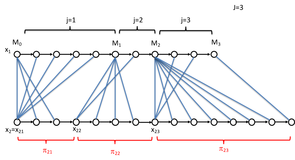
Figure 14: Example of schema for the Proof of Theorem 6.1, for $J=3$. Relation $B$ is shown as blue segments.

Let $M_{0}=0$, $x_{21}=x_{2}$. Now let $M_{1}$ be the greatest $m_{1}$ such that $m_{1}\leq\mathtt{len}(\pi_{1})$ and $(\pi_{1}(i_{1}),x_{21})\in B$ for all $i_{1}\in\{\iota\,|\,M_{0}\leq\iota<m_{1}\}$, recalling that $(\pi_{1}(M_{0}),x_{21})\in B$ by hypothesis. Moreover, since $(\pi_{1}(M_{0}),x_{21})\in B$ and $B$ is a CoPa-bisimulation, by Condition 2 of Definition 23, there exists $\pi_{21}\in\mathtt{BPaths^{F}}(x_{21})$ such that $(\pi_{1}(M_{0}),\pi_{21}(i_{2}))\in B$ for all $i_{2}\in\{\iota\,|\,0\leq\iota<\mathtt{len}(\pi_{21})\}$ and $(\pi_{1}(M_{1}),\pi_{21}(x_{22}))\in B$, where $x_{22}=\pi_{21}(\mathtt{len}(\pi_{21}))$. Furthermore, since $\mathcal{M},\pi_{1}(M_{0})\models\Phi_{2}$, by the I.H. we get that also $\mathcal{M},\pi_{21}(i_{2})\models\Phi_{2}$ for all $i_{2}\in\{\iota\,|\,0\leq\iota<\mathtt{len}(\pi_{21})\}$.

For $j>1$, let $M_{j}$ be the greatest $m_{j}$ such that $m_{j}\leq\mathtt{len}(\pi_{1})$ and $(\pi_{1}(i_{1}),x_{2j})$ $\in$ $B$ for all $i_{1}\in\{\iota\,|\,Z_{j-1}\leq\iota<z_{j}\}$ recalling that $(\pi_{1}(M_{j-1}),x_{2j})\in B$ by definition of $\pi_{2j-1}$. Moreover, since $(\pi_{1}(M_{j-1}),x_{2j})\in B$ and $B$ is a CoPa-bisimulation, by Condition 2 of Definition 23, there exists $\pi_{2j}\in\mathtt{BPaths^{F}}(x_{2j})$ such that $(\pi_{1}(M_{j-1}),\pi_{2j}(i_{2}))\in B$ for all $i_{2}\in\{\iota\,|\,0\leq\iota<\mathtt{len}(\pi_{2j})\}$ and $(\pi_{1}(M_{j}),\pi_{2j}(x_{2(j+1)}))\in B$, where $x_{2(j+1)}=\pi_{2j}(\mathtt{len}(\pi_{2j}))$. Furthermore, since $\mathcal{M},\pi_{1}(M_{j-1})\models\Phi_{2}$, by the I.H. we get that also $\mathcal{M},\pi_{2j}(i_{2})\models\Phi_{2}$ for all $i_{2}\in\{\iota\,|\,0\leq\iota<\mathtt{len}(\pi_{2j})\}$.

Finally, letting $J$ be the greatest $j$ as above, since $\mathcal{M},\pi_{1}(M_{J})\models\Phi_{1}$, by the I.H. we get that also $\mathcal{M},\pi_{2J}(\mathtt{len}(\pi_{2J}))\models\Phi_{1}$.

We note that $\pi_{2j}(0)=\pi_{2(j-1)}(\mathtt{len}(\pi_{2(j-1)}))$ for $j=1\ldots J$. Thus we can build the following path $\pi_{2}$:

$$\pi_{2}(n)=\left\{\begin{array}[]{l}\pi_{21}(n),\mbox{ if }n\in[0,\mathtt{len}(\pi_{21})),\\ \vdots\\ \pi_{2j}(n-\sum_{i=1}^{j-1}\mathtt{len}(\pi_{2i})),\mbox{ if }n\in\left[\sum_{i=1}^{j-1}\mathtt{len}(\pi_{2i}),\sum_{i=1}^{j}\mathtt{len}(\pi_{2i})\right),\\ \vdots\\ \pi_{2J}(n-\sum_{i=1}^{J-1}\mathtt{len}(\pi_{2i})),\mbox{ if }n\geq\sum_{i=1}^{j}\mathtt{len}(\pi_{2i}).\end{array}\right.$$

Clearly, $\pi_{2}\in\mathtt{BPaths^{F}}(x_{2})$ since $\pi_{2}(0)=\pi_{2,1}(0)=x_{2}$ because $\pi_{21}\in\mathtt{BPaths^{F}}(x_{2})$ and $\pi_{2J}$ is bounded. Moreover, by construction, $\mathcal{M},\pi_{2}(i_{2})\models\Phi_{2}$ for all $i_{2}\in\{\iota\,|\,0\leq\iota<\mathtt{len}(\pi_{2})\}$ and $\mathcal{M},\pi_{2}(\mathtt{len}(\pi_{2}))\models\Phi_{1}$. Thus $\mathcal{M},x_{2}\models\stackrel{{\scriptstyle\rightarrow}}{{\zeta}}\Phi_{1}[\Phi_{2}]$.

0.E.4 Proof of Theorem 6.2

We have to prove that Conditions 1-5 of the Definition 23 are fullfilled. We consider only Condition 2, since the proof for Conditions 3-5 is similar and that of Condition 1 is trivial. We proceed by contradition. Suppose Condition 2 is not satisfied; this means that there exists $\bar{\pi}\in\mathtt{BPaths^{F}}(x_{1})$ such that $(\bar{\pi}(i),x_{2})\in\simeq_{{\tt ICRL}}$ for all $i\in\{\iota\,|\,0\leq\iota<\mathtt{len}(\bar{\pi})\}$ and, for all $\pi\in\mathtt{BPaths^{F}}(x_{2})$, having considered that $\pi(0)=x_{2}\,\simeq_{{\tt ICRL}}\,x_{1}$, the following holds:
$(\bar{\pi}(\mathtt{len}(\bar{\pi})),\pi(\mathtt{len}(\pi)))\not\in\simeq_{{\tt ICRL}}$ or there exists $h_{\pi}$ such that $0<h_{\pi}<\mathtt{len}(\pi)$ and $(x_{1},\pi(h_{\pi}))\not\in\simeq_{{\tt ICRL}}$. Let set $I$ be defined as

$I=\{\pi\in\mathtt{BPaths^{F}}(x_{2})\,|\,\mbox{there exists }h_{\pi}\mbox{ such that }0<h_{\pi}<\mathtt{len}(\pi)$
                                                                  $\mbox{ and }(x_{1},\pi(h_{\pi}))\not\in\simeq_{{\tt ICRL}}\}$

and, for each $\pi\in I$, let $\Omega^{I}_{\pi}$ be a formula such that $\mathcal{M},x_{1}\models\Omega^{I}_{\pi}$ and $\mathcal{M},\pi(h_{\pi})\not\models\Omega^{I}_{\pi}$—such a formula exists because $(x_{1},\pi(h_{\pi}))\not\in\simeq_{{\tt ICRL}}$.

Let furthermore set $L$ be defined as

$$L=\{\pi\in\mathtt{BPaths^{F}}(x_{2})\,|\,(\bar{\pi}(\mathtt{len}(\bar{\pi})),\pi(\mathtt{len}(\pi)))\not\in\simeq_{{\tt ICRL}}\}$$

and, for each $\pi\in L$, let $\Omega^{L}_{\pi}$ be a formula such that $\mathcal{M},\bar{\pi}(\mathtt{len}(\bar{\pi}))\models\Omega^{L}_{\pi}$ and $\mathcal{M},\pi(\mathtt{len}(\pi))\not\models\Omega^{L}_{\pi}$—such a formula exists because $(\bar{\pi}(\mathtt{len}(\bar{\pi})),\pi(\mathtt{len}(\pi)))\not\in\simeq_{{\tt ICRL}}$. Note that $I\cup L=\mathtt{BPaths^{F}}(x_{2})$ by hypothesis. Clearly, $\mathcal{M},x_{1}\models\bigwedge_{\pi\in I}\Omega^{I}_{\pi}$ and, since $(\bar{\pi}(i),x_{2})\in\simeq_{{\tt ICRL}}$ for all $i\in\{\iota\,|\,0\leq\iota<\mathtt{len}(\bar{\pi})\}$, we also get $\mathcal{M},\bar{\pi}(i)\models\bigwedge_{\pi\in I}\Omega^{I}_{\pi}$ for all $i\in\{\iota\,|\,0\leq\iota<\mathtt{len}(\bar{\pi})\}$—recall that $\bar{\pi}(0)=x_{1}$. Also, $\mathcal{M},\bar{\pi}(\mathtt{len}(\bar{\pi}))\models\bigwedge_{\pi\in L}\Omega^{L}_{\pi}$

Thus, we get $\mathcal{M},x_{1}\models\Psi$, where $\Psi$ is the formula $\stackrel{{\scriptstyle\rightarrow}}{{\zeta}}(\bigwedge_{\pi\in L}\Omega^{L}_{\pi})[\bigwedge_{\pi\in I}\Omega^{I}_{\pi}]$. On the other hand, $\mathcal{M},x_{2}\not\models\Psi$, since, for every path $\pi\in\mathtt{BPaths^{F}}(x_{2})$, $\pi(h_{\pi})$ does not satisfy $\bigwedge_{\pi\in I}\Omega^{I}_{\pi}$ for some $h_{\pi}$ with $0<h_{\pi}<\mathtt{len}(\pi)$—by construction of $\bigwedge_{\pi\in I}\Omega^{I}_{\pi}$—or $\pi(\mathtt{len}(\pi))$ does not satisfy $\bigwedge_{\pi\in L}\Omega^{L}_{\pi}$—by construction of $\bigwedge_{\pi\in L}\Omega^{L}_{\pi}$. In conclusion, we have found a formula, $\Psi$, such that $\mathcal{M},x_{1}\models\Psi$ whereas $\mathcal{M},x_{2}\not\models\Psi$ and this contradicts $x_{1}\,\simeq_{{\tt ICRL}}\,x_{2}$.

References

- [1] Bartocci, E., Bortolussi, L., Loreti, M., Nenzi, L.: Monitoring mobile and spatially distributed cyber-physical systems. In: MEMOCODE. pp. 146–155. ACM (2017)
- [2] Belmonte, G., Broccia, G., Ciancia, V., Latella, D., Massink, M.: Using spatial logic and model checking for nevus segmentation. CoRR abs/2012.13289 (2020), https://arxiv.org/abs/2012.13289, “(to appear in the Proceedings of FormaliSE 2021 with title Feasibility of Spatial Model Checking for Nevus Segmentation)”
- [3] Belmonte, G., Ciancia, V., Latella, D., Massink, M.: Innovating medical image analysis via spatial logics. In: ter Beek, M.H., Fantechi, A., Semini, L. (eds.) From Software Engineering to Formal Methods and Tools, and Back - Essays Dedicated to Stefania Gnesi on the Occasion of Her 65th Birthday. Lecture Notes in Computer Science, vol. 11865, pp. 85–109. Springer (2019), https://doi.org/10.1007/978-3-030-30985-5_7
- [4] Belmonte, G., Ciancia, V., Latella, D., Massink, M.: Voxlogica: A spatial model checker for declarative image analysis. In: Vojnar, T., Zhang, L. (eds.) Tools and Algorithms for the Construction and Analysis of Systems - 25th International Conference, TACAS 2019, Held as Part of the European Joint Conferences on Theory and Practice of Software, ETAPS 2019, Prague, Czech Republic, April 6-11, 2019, Proceedings, Part I. Lecture Notes in Computer Science, vol. 11427, pp. 281–298. Springer (2019), https://doi.org/10.1007/978-3-030-17462-0_16
- [5] van Benthem, J., Bezhanishvili, G.: Modal logics of space. In: Aiello, M., Pratt-Hartmann, I., van Benthem, J. (eds.) Handbook of Spatial Logics, pp. 217–298. Springer (2007), https://doi.org/10.1007/978-1-4020-5587-4_5
- [6] van Benthem, J., Bezhanishvili, N., Enqvist, S., Yu, J.: Instantial neighbourhood logic. Rev. Symb. Log. 10(1), 116–144 (2017), https://doi.org/10.1017/S1755020316000447
- [7] Browne, M.C., Clarke, E.M., Grumberg, O.: Characterizing finite kripke structures in propositional temporal logic. Theor. Comput. Sci. 59, 115–131 (1988), https://doi.org/10.1016/0304-3975(88)90098-9
- [8] Buonamici, F.B., Belmonte, G., Ciancia, V., Latella, D., Massink, M.: Spatial logics and model checking for medical imaging. Int. J. Softw. Tools Technol. Transf. 22(2), 195–217 (2020), https://doi.org/10.1007/s10009-019-00511-9
- [9] Ciancia, V., Gilmore, S., Grilletti, G., Latella, D., Loreti, M., Massink, M.: Spatio-temporal model checking of vehicular movement in public transport systems. Int. J. Softw. Tools Technol. Transf. 20(3), 289–311 (2018), https://doi.org/10.1007/s10009-018-0483-8
- [10] Ciancia, V., Grilletti, G., Latella, D., Loreti, M., Massink, M.: An experimental spatio-temporal model checker. In: Bianculli, D., Calinescu, R., Rumpe, B. (eds.) Software Engineering and Formal Methods - SEFM 2015 Collocated Workshops: ATSE, HOFM, MoKMaSD, and VERY*SCART, York, UK, September 7-8, 2015, Revised Selected Papers. Lecture Notes in Computer Science, vol. 9509, pp. 297–311. Springer (2015), https://doi.org/10.1007/978-3-662-49224-6_24
- [11] Ciancia, V., Latella, D., Loreti, M., Massink, M.: Specifying and verifying properties of space. In: Díaz, J., Lanese, I., Sangiorgi, D. (eds.) Theoretical Computer Science - 8th IFIP TC 1/WG 2.2 International Conference, TCS 2014, Rome, Italy, September 1-3, 2014. Proceedings. Lecture Notes in Computer Science, vol. 8705, pp. 222–235. Springer (2014), https://doi.org/10.1007/978-3-662-44602-7_18
- [12] Ciancia, V., Latella, D., Loreti, M., Massink, M.: Model checking spatial logics for closure spaces. Log. Methods Comput. Sci. 12(4) (2016), https://doi.org/10.2168/LMCS-12(4:2)2016
- [13] Ciancia, V., Latella, D., Massink, M.: Embedding RCC8D in the collective spatial logic CSLCS. In: Boreale, M., Corradini, F., Loreti, M., Pugliese, R. (eds.) Models, Languages, and Tools for Concurrent and Distributed Programming - Essays Dedicated to Rocco De Nicola on the Occasion of His 65th Birthday. Lecture Notes in Computer Science, vol. 11665, pp. 260–277. Springer (2019), https://doi.org/10.1007/978-3-030-21485-2_15
- [14] Ciancia, V., Latella, D., Massink, M., de Vink, E.: Towards spatial bisimilarity for closure models: Logical and coalgebraic characterisations (2020), https://arxiv.org/pdf/2005.05578.pdf
- [15] De Nicola, R., Montanari, U., Vaandrager, F.W.: Back and forth bisimulations. In: Baeten, J.C.M., Klop, J.W. (eds.) CONCUR ’90, Theories of Concurrency: Unification and Extension, Amsterdam, The Netherlands, August 27-30, 1990, Proceedings. Lecture Notes in Computer Science, vol. 458, pp. 152–165. Springer (1990), https://doi.org/10.1007/BFb0039058
- [16] Galton, A.: A generalized topological view of motion in discrete space. Theoretical Computer Science. Elsevier. 305((1-3)), 111–134 (2003)
- [17] Groote, J.F., Jansen, D.N., Keiren, J.J.A., Wijs, A.: An O(mlogn) algorithm for computing stuttering equivalence and branching bisimulation. ACM Trans. Comput. Log. 18(2), 13:1–13:34 (2017), https://doi.org/10.1145/3060140
- [18] Hansen, H.: Monotonic Modal Logics (2003), Master’s Thesis, ILLC, University of Amsterdam.
- [19] Linker, S., Papacchini, F., Sevegnani, M.: Analysing spatial properties on neighbourhood spaces. In: Esparza, J., Král’, D. (eds.) 45th International Symposium on Mathematical Foundations of Computer Science, MFCS 2020, August 24-28, 2020, Prague, Czech Republic. LIPIcs, vol. 170, pp. 66:1–66:14. Schloss Dagstuhl - Leibniz-Zentrum für Informatik (2020), https://doi.org/10.4230/LIPIcs.MFCS.2020.66
- [20] Morris, S.: Topology Without Tears (2020), https://www.topologywithouttears.net accessed on Mar. 2, 2021
- [21] Nenzi, L., Bortolussi, L., Ciancia, V., Loreti, M., Massink, M.: Qualitative and quantitative monitoring of spatio-temporal properties with SSTL. Logical Methods in Computer Science 14(4) (2018)
- [22] Randell, D.A., Landini, G., Galton, A.: Discrete mereotopology for spatial reasoning in automated histological image analysis. IEEE Trans. Pattern Anal. Mach. Intell. 35(3), 568–581 (2013), https://doi.org/10.1109/TPAMI.2012.128
- [23] Tsigkanos, C., Kehrer, T., Ghezzi, C.: Modeling and verification of evolving cyber-physical spaces. In: ESEC/SIGSOFT FSE. pp. 38–48. ACM (2017)