One colorful resolution to the neutrino mass generation, three lepton flavor universality anomalies, and the Cabibbo angle anomaly

Abstract

We propose a simple model to simultaneously explain four observed flavor anomalies while generating the neutrino mass at the one-loop level. Specifically, we address the measured anomalous magnetic dipole moments of the muon, $\Delta a_{\mu}$ , and electron, $\Delta a_{e}$, the observed anomaly of $b\rightarrow sl^{+}l^{-}$ in the $B$-meson decays, and the Cabibbo-angle anomaly. The model consists of four colorful new degrees of freedom: three scalar leptoquarks with the Standard Model quantum numbers $(3,3,-1/3),(3,2,1/6)$, and $(3,1,2/3)$, and one pair of down-quark-like vector fermion in $(3,1,-1/3)$. The baryon number is assumed to be conserved for simplicity.

Phenomenologically viable solutions with the minimal number of real parameters can be found to accommodate all the above-mentioned anomalies and produce the approximate, close to $1\sigma$, neutrino oscillation pattern at the same time. From general consideration, the model robustly predicts: (1) neutrino mass is of the normal hierarchy type, and (2) ${\cal M}^{\nu}_{ee}\lesssim 3\times 10^{-4}\mathrm{eV}$.

The possible UV origin to explain the flavor pattern of the found viable parameter space is briefly discussed. The parameter space can be well reproduced within a simple split fermion toy model.

I Introduction

Despite of the amazing success of the Standard Model (SM) of particle physics, new physics (NP) beyond the SM is ineluctable because compelling evidence showing that at least two active neutrinos are massive[1]. In addition to the nonzero neutrino masses, several recent experimental measurements prominently deviated from the SM predictions are also suggestive to NP. In particular,

• The measured anomalous magnetic moment of muon $(g-2)_{\mu}$[1, 2] differs from the most recent SM prediction[3, 4] by an amount of $\sim 3.7\sigma$:

  $$\triangle a_{\mu}=a_{\mu}^{exp}-a_{\mu}^{SM}\simeq(27.4\pm 7.3)\times 10^{-10}\,,$$ (1)

  where the uncertainty is the quadratic combination of the experimental and theoretical ones. The most recent $0.46ppm$ measurement conducted at Fermilab[5] gives

  $$a_{\mu}^{exp}=116592040(54)\times 10^{-11}\,,$$ (2)

  which agrees with the previous measurements. And the new experimental average of $a_{\mu}^{exp}=116592061(41)\times 10^{-11}$ drives the deviation to $4.2\sigma$ with

  $$\triangle a_{\mu}\simeq(25.1\pm 5.9)\times 10^{-10}\,.$$ (3)

  Another new measurement at the J-PARC[6] is also expected to improve the experimental uncertainty in the near future.

• With the determination of the fine-structure constant by using the cesium atom[7], the measured electron $(g-2)_{e}$ [8] shows a $\sim 2.4\sigma$ discrepancy from the SM prediction[9]:

  $$\triangle a_{e}^{Cs}=a_{e}^{exp}-a_{e}^{SM}\simeq(-8.7\pm 3.6)\times 10^{-13}\,.$$ (4)

  Note that $\triangle a_{e}^{Cs}$ and $\triangle a_{\mu}$ have opposite signs. New models[10, 11, 12, 13, 14, 15, 16, 17, 18, 19, 20, 21, 22, 23, 24, 25, 26, 27, 28, 29, 30] have been constructed to accommodate both $\triangle a_{e}^{Cs}$ and $\triangle a_{\mu}$. Moreover, [31, 32, 33] also attempt to incorporate the neutrino mass generation with the observed $\triangle a_{e,\mu}$.

  However, the most recent $\alpha$ determination by using the rubidium atom[34] yields a different outcome

  $$\triangle a_{e}^{Rb}\simeq(+4.8\pm 3.0)\times 10^{-13}\,,$$ (5)

  whose sign is different from the one of $\triangle a_{e}^{Cs}$. These two highly precise values of $\alpha$ differ by a tantalizing $\sim 5\sigma$. More independent investigations or measurements are required to resolve this tension. At this moment, we should consider both cases in this work.

• From the global fits[35, 36, 37, 38, 39, 40, 41, 42, 43, 44, 45, 46] to various $b\rightarrow sl^{+}l^{-}$ data[47, 48, 49, 50, 51, 52, 53, 54, 55, 56, 57, 58, 59, 60, 61], the discrepancy is more than $5\sigma$ from the SM predictions. The new result[62] further strengthens the lepton flavor universality violation[63, 64]. This anomaly alone convincingly indicates NP, and stimulates many investigations to address this deviation. For example, a new gauge sector was introduced in [65, 66, 67], leptoquark has been employed in [68, 69, 70, 71, 72, 73, 74, 75, 76], assisted by the 1-loop contributions from exotic particles in [77, 78, 79, 80, 81], and more references can be found in [35, 82, 83].

• The so-called Cabibbo angle anomaly refers to the unexpected shortfall in the first row Cabibbo-Kobayashi-Maskawa(CKM) unitarity[1],

  $$|V_{ud}|^{2}+|V_{us}|^{2}+|V_{ub}|^{2}=0.9985\pm 0.0005\,.$$ (6)

  The above value is smaller than one, and the inconsistence is now at the level of $\simeq 2-4\sigma$ level[84, 85]. There are tensions among different determinations of the Cabibbo angle from tau decays[86], kaon decays[87], and super-allowed $\beta$ decay (by using CKM unitarity and the theoretical input[88, 89]). The potential NP involving vector quarks or the origins of lepton flavor universality violation have been discussed in [90, 91, 92, 93, 94, 95, 96, 97, 98].

Whether these $2-5\,\sigma$ anomalies will persist is not predictable; the future improvement on the theoretical predictions and the experimental measurements will be the ultimate arbiters. However, at this moment, it is interesting to speculate whether all the above-mentioned anomalies and the neutrino mass can be explained simultaneously. In this paper, we point out one of such resolutions. With the addition of three scalar leptoquarks, $T(3,3,-1/3)$, $D(3,2,1/6)$, and $S(3,1,2/3)$, and a pair of vector fermion, $b^{\prime}_{L,R}(3,1,-1/3)$, the plethoric new parameters ( mostly the Yukawa couplings) allow one to reconcile all data contemporarily. Parts of the particle content of this model had been employed in the past to accommodate some of the anomalies. However, to our best knowledge, this model as whole is new to comprehensively interpret all the observed deviations from the SM.

The paper is laid out as follows: in Sec.II we spell out the model and the relevant ingredients. Following that in Sec.III we explain how each anomaly and the neutrino mass generation works in our model. Next we discuss the various phenomenological constraint and provide some model parameter samples in Sec.IV . In Sec.V we discuss some phenomenological consequences, and the UV origin of the flavor pattern of the parameter space. Then comes our conclusion in Sec.VI. Some details of our notation and the low energy effective Hamiltonian are collected in the Appendix.

II The Model

In this model, three scalar leptoquarks, $T(3,3,-1/3)$, $D(3,2,1/6)$, and $S(3,1,2/3)$. , and a pair of down-quark-like vector fermion, $b^{\prime}_{L,R}(3,1,-1/3)$, are augmented on top of the SM. Our notation for the SM particle content and the exotics are listed in Tab.1 and Tab.2, respectively.

	SM Fermion					SM Scalar
Fields	$Q_{L}=\begin{pmatrix}u_{L}\\ d_{L}\end{pmatrix}$	$u_{R}$	$d_{R}$	$L_{L}=\begin{pmatrix}\nu_{L}\\ e_{L}\end{pmatrix}$	$e_{R}$	$H=\begin{pmatrix}H^{+}\\ H^{0}\end{pmatrix}$
$SU(3)_{c}$	$3$	$3$	$3$	$1$	$1$	$1$
$SU(2)_{L}$	$2$	$1$	$1$	$2$	$1$	$2$
$U(1)_{Y}$	$\frac{1}{6}$	$\frac{2}{3}$	$-\frac{1}{3}$	$-\frac{1}{2}$	$-1$	$\frac{1}{2}$

Table 1: The SM field content and quantum number assignment under the SM gauge symmetries $SU(3)_{c}\otimes SU(2)_{L}\otimes U(1)_{Y}$, where $L,R$ stand for the chirality of the fermion. For simplicity, all the generation indices associated with the fermions are suppressed.

	New Fermion	New Scalar
Fields	$b^{\prime}_{L,R}$	$T=\begin{pmatrix}T^{\frac{2}{3}}\\ T^{-\frac{1}{3}}\\ T^{-\frac{4}{3}}\end{pmatrix}$	$D=\begin{pmatrix}D^{\frac{2}{3}}\\ D^{-\frac{1}{3}}\end{pmatrix}$	$S^{\frac{2}{3}}$
$SU(3)_{c}$	$3$	$3$	$3$	$3$
$SU(2)_{L}$	$1$	$3$	$2$	$1$
$U(1)_{Y}$	$-\frac{1}{3}$	$-\frac{1}{3}$	$\frac{1}{6}$	$\frac{2}{3}$
lepton number	$0$	$1$	$-1$	$-1$
baryon number	$\frac{1}{3}$	$\frac{1}{3}$	$\frac{1}{3}$	$\frac{1}{3}$

Table 2: New field content and quantum number assignment under the SM gauge symmetries $SU(3)_{c}\otimes SU(2)_{L}\otimes U(1)_{Y}$, and the global lepton/baryon numbers.

Like most models beyond the SM, the complete Lagrangian is lengthy, and not illuminating. In this work, we only focus on the new gauge invariant interactions relevant to addressing the flavor anomalies. For simplicity, we also assume the model Lagrangian respects the global baryon number symmetry, and both $T$ and $S$ carry one third of baryon-number to avoid their possible di-quark couplings. Moreover, we do not consider the possible CP violating signals in this model.

For the scalar couplings, we have

$${\cal L} \supset \mu_{3}\left\{H,\tilde{D}\right\}\odot T+\mu_{1}\left[H,D\right]S^{-\frac{2}{3}}+H.c.$$ (8)

$$= \mu_{3}\left[H^{+}D^{\frac{1}{3}}T^{-\frac{4}{3}}-\frac{1}{\sqrt{2}}\left(H^{0}D^{\frac{1}{3}}-H^{+}D^{-\frac{2}{3}}\right)T^{-\frac{1}{3}}-H^{0}D^{-\frac{2}{3}}T^{\frac{2}{3}}\right]$$

$$-\mu_{1}\frac{1}{\sqrt{2}}\left(H^{0}D^{\frac{2}{3}}-H^{+}D^{-\frac{1}{3}}\right)S^{-\frac{2}{3}}+H.c.$$

The couplings $\mu_{1}$ and $\mu_{3}$ are unknown dimensionful parameters. Note that the $\mu_{3}$ coupling softly breaks the global lepton number by two units, which is crucial for the neutrino mass generation. On the other hand, the lepton-number conserving $\mu_{1}$ triple scalar interaction is essential for explaining $\triangle a_{e}$ and $\triangle a_{\mu}$ ( to be discussed in the following sections). As it will be clear later, to fit all the data, $\mu_{3}$ turns out to be very small, $\sim{\cal O}(0.5\mathrm{keV})$, and $\mu_{1}\sim{\cal O}(\mathrm{TeV})$.

After electroweak spontaneous symmetry breaking (SSB), $\langle H^{0}\rangle=v_{0}/\sqrt{2}$ and the Goldstone $H^{\pm}$ are eaten by the $W^{\pm}$ bosons. Below the electroweak scale, it becomes:

$$-\frac{\mu_{3}v_{0}}{2}D^{\frac{1}{3}}T^{-\frac{1}{3}}-\frac{\mu_{3}v_{0}}{\sqrt{2}}D^{-\frac{2}{3}}T^{\frac{2}{3}}-\frac{\mu_{1}v_{0}}{2}D^{\frac{2}{3}}S^{-\frac{2}{3}}+H.c.$$ (9)

Comparing to their tree-level masses, $\widetilde{M}_{T,D,S}\simeq M_{LQ}$, we expect the mixings are small and suppressed by the factor of ${\cal O}(\mu_{LQ}v_{0}/M_{LQ}^{2})$. However, these mixings break the isospin multiplet mass degeneracy of $T$ and $D$. After the mass diagonalization, we have two charge-$\frac{1}{3}$, three charge-$\frac{2}{3}$, and one charge-$\frac{4}{3}$ physical scalar leptoquarks.

In addition to the SM Yukawa interactions in the form of $\bar{Q}d_{R}H$, $\bar{Q}u_{R}\tilde{H}$, and $\bar{L}e_{R}H$, this model has the following new Yukawa couplings ( in the interaction basis):

$${\cal L} \supset -\widetilde{\lambda}_{T}T^{\dagger}\cdot\left\{\bar{L}^{c},Q\right\}-\widetilde{\lambda}_{D}\bar{d}_{R}\left[L,D\right]-\widetilde{\lambda}^{\prime}_{D}\bar{b^{\prime}}_{R}\left[L,D\right]-\widetilde{\lambda}_{S}\bar{e}_{R}b^{\prime}_{L}S^{-\frac{2}{3}}-\widetilde{Y}_{d}^{\prime}\bar{Q}b^{\prime}_{R}H+H.c.$$ (11)

$$= -\widetilde{\lambda}_{T}\left[\bar{\nu}^{c}u_{L}T^{-\frac{2}{3}}+\left(\bar{\nu}^{c}d_{L}+\bar{e}^{c}u_{L}\right)\frac{T^{\frac{1}{3}}}{\sqrt{2}}+\bar{e}^{c}d_{L}T^{\frac{4}{3}}\right]-\widetilde{Y}_{d}^{\prime}(\bar{u}_{L}H^{+}+\bar{d}_{L}H^{0})b^{\prime}_{R}$$

$$-\widetilde{\lambda}_{D}\frac{\bar{d}_{R}}{\sqrt{2}}\left(\nu_{L}D^{-\frac{1}{3}}-e_{L}D^{\frac{2}{3}}\right)-\widetilde{\lambda}^{\prime}_{D}\frac{\bar{b^{\prime}}_{R}}{\sqrt{2}}\left(\nu_{L}D^{-\frac{1}{3}}-e_{L}D^{\frac{2}{3}}\right)-\widetilde{\lambda}_{S}\bar{e}_{R}b^{\prime}_{L}S^{-\frac{2}{3}}+H.c.\,,$$

where all the generation indices are suppressed to keep the notation simple and it should be understood that all the Yukawa couplings are matrices. Moreover, the model allows two kinds of tree-level Dirac mass term:

$${\cal L}\supset M_{1}\bar{b}^{\prime}_{R}b^{\prime}_{L}+M_{2}\bar{d}_{R}b^{\prime}_{L}+H.c.$$ (12)

With the introduction of $b^{\prime}$, the mass matrix for down-quark-like fermions after the electroweak SSB becomes:

$${\cal L}\supset-(\bar{d_{R}},\bar{b^{\prime}_{R}}){\cal M}^{d}\left(\begin{array}[]{c}d_{L}\\ b^{\prime}_{L}\end{array}\right)+H.c.\,,\,\,{\cal M}^{d}=\left(\begin{array}[]{cc}\frac{\widetilde{Y}_{d}v_{0}}{\sqrt{2}}&M_{2}\\ \frac{\widetilde{Y}^{\prime}_{d}v_{0}}{\sqrt{2}}&M_{1}\\ \end{array}\right)\,,$$ (13)

where $\widetilde{Y}_{d}$ is the SM down-quark three-by-three Yukawa coupling matrix in the interaction basis. Note that ${\cal M}^{d}$ is now a four-by-four matrix. This matrix can be diagonalized by the bi-unitary transformation, ${\cal M}^{d}_{diag}=U^{d}_{R}{\cal M}^{d}(U^{d}_{L})^{\dagger}=\mbox{diag}(m_{d},m_{s},m_{b},M_{b^{\prime}})$, and

$$U^{d}_{R}{\cal M}^{d}({\cal M}^{d})^{\dagger}(U^{d}_{R})^{\dagger}=U^{d}_{L}({\cal M}^{d})^{\dagger}{\cal M}^{d}(U^{d}_{L})^{\dagger}=({\cal M}_{diag}^{d})^{2}\,,$$ (14)

$$(d_{1},d_{2},d_{3},d_{4})_{L/R}=(d,s,b,b^{\prime})_{L/R}(U^{d}_{L/R})^{*}\,,$$ (15)

where $(d_{1},d_{2},d_{3},d_{4})$ and $(d,s,b,b^{\prime})$ stand for the interaction and mass eigenstates, respectively. The new notation, $d_{4}$, is designated for the interaction basis of the singlet $b^{\prime}_{L,R}$, and $b^{\prime}$ is recycled to represent the heaviest mass eigenstate of down-type quark. One will see that the mass and interaction eigenstates of $b^{\prime}$ are very close to each other from the later phenomenology study.

Similarly, the SM up-type quarks and the charged leptons can be brought to their mass eigenstates by $U^{u}_{L/R}$ and $U^{e}_{L/R}$, respectively. Since $\widetilde{\lambda}$’s are unknown in the first place, one can focus on the couplings in the charged fermion mass basis, denoted as $\lambda^{T,D,S}$, which are more phenomenologically useful. However, note that the mass diagonalization matrices are in general different for the left-handed (LH) up- and LH down-quark sectors. If we pick the flavor indices of $\lambda^{T}$ to label the charged lepton and down quark mass states, the up-type quark in the triplet leptoquark coupling will receive an extra factor to compensate the difference between $U^{d}_{L}$ and $U^{u}_{L}$. Explicitly,

$${\cal L}\supset - \sum_{l=e,\mu,\tau}\sum_{p=d,s,b,b^{\prime}}(\lambda^{T})_{lp}\sum_{r=u,c,t}\tilde{A}^{\dagger}_{pr}\left[\bar{\nu}_{l}^{c}T^{-\frac{2}{3}}+\bar{e}_{l}^{c}\frac{T^{\frac{1}{3}}}{\sqrt{2}}\right]u_{L,r}$$ (16)

$$- \sum_{l=e,\mu,\tau}\sum_{p=d,s,b,b^{\prime}}(\lambda^{T})_{lp}\left[\bar{e}_{l}^{c}T^{\frac{4}{3}}+\bar{\nu}_{l}^{c}\frac{T^{\frac{1}{3}}}{\sqrt{2}}\right]d_{L,p}+H.c.$$

with the four-by-three matrix

$$\tilde{A}^{\dagger}_{pr}=\sum_{j=1}^{4}(U^{d}_{L})_{pj}(U^{u}_{L})^{\dagger}_{jr}\,.$$ (17)

As will be discussed in below, $\tilde{A}$ is the extended CKM rotation matrix, $\tilde{V}$, and $\tilde{A}\rightarrow(V_{CKM})$ if $b^{\prime}_{L}$ decouples. Now, all $\lambda^{T}$, $\lambda^{D}$, and $\lambda^{S}$ are three-by-four matrices.

In the interaction basis, only the LH doublets participate in the charged-current(CC) interaction. Thus, the SM $W^{\pm}$ interaction for the quark sector is

$${\cal L}\supset\frac{g_{2}}{\sqrt{2}}\sum_{i=1}^{3}\left(\bar{u}_{i}\gamma^{\alpha}\hat{L}d_{i}\right)W^{+}_{\alpha}+H.c.$$ (18)

However, the singlet $b^{\prime}_{L}$ mixes with other LH down-type-quarks and change the SM CC interaction. In the mass basis, it becomes

$${\cal L}\supset\frac{g_{2}}{\sqrt{2}}(\bar{u},\bar{c},\bar{t})\gamma^{\alpha}\hat{L}\widetilde{V}\left(\begin{array}[]{c}d\\ s\\ b\\ b^{\prime}\end{array}\right)W^{+}_{\alpha}+H.c.$$ (19)

where

$$\widetilde{V}=\left(\begin{array}[]{cccc}\widetilde{V}_{ud}&\widetilde{V}_{us}&\widetilde{V}_{ub}&\widetilde{V}_{ub^{\prime}}\\ \widetilde{V}_{cd}&\widetilde{V}_{cs}&\widetilde{V}_{cb}&\widetilde{V}_{cb^{\prime}}\\ \widetilde{V}_{td}&\widetilde{V}_{ts}&\widetilde{V}_{tb}&\widetilde{V}_{tb^{\prime}}\\ \end{array}\right)\,,\;\mbox{ and }\,\,\widetilde{V}_{pq}\equiv\sum_{i=1}^{3}(U^{u}_{L})_{pi}(U^{d}_{L})^{\dagger}_{iq}\,.$$ (20)

Therefore, the SM three-by-three unitary CKM matrix changes into a three-by-four matrix in our model. When the $b^{\prime}_{L}$ decouples, the coupling matrix $\widetilde{V}$ reduces to the SM $V_{CKM}$.

Instead of dealing with a three-by-four matrix, it is helpful to consider an auxiliary unitary four-by-four matrix

$$\widetilde{V}_{4}\equiv\left(\begin{array}[]{cc}U^{u}_{L}&0\\ 0&1\end{array}\right)\cdot(U^{d}_{L})^{\dagger}=\left(\begin{array}[]{cccc}\widetilde{V}_{ud}&\widetilde{V}_{us}&\widetilde{V}_{ub}&\widetilde{V}_{ub^{\prime}}\\ \widetilde{V}_{cd}&\widetilde{V}_{cs}&\widetilde{V}_{cb}&\widetilde{V}_{cb^{\prime}}\\ \widetilde{V}_{td}&\widetilde{V}_{ts}&\widetilde{V}_{tb}&\widetilde{V}_{tb^{\prime}}\\ (U^{d}_{L})_{d4}^{*}&(U^{d}_{L})_{s4}^{*}&(U^{d}_{L})_{b4}^{*}&(U^{d}_{L})_{b^{\prime}4}^{*}\\ \end{array}\right)\,.$$ (21)

To quantify the NP effect, one can parameterize the four-by-four unitary matrix $U^{d}_{L}$ by a unitary three-by-three sub-matrix, $U^{d}_{L3}$, and three rotations as:

$$(U^{d}_{L})^{\dagger}=\left(\begin{array}[]{cc}(U^{d}_{L3})^{\dagger}&0\\ 0&1\\ \end{array}\right)\cdot R_{4}\,,\;\;\mbox{where}\;\;R_{4}=\left(\begin{array}[]{cccc}c_{1}&0&0&s_{1}\\ -s_{1}s_{2}&c_{2}&0&c_{1}s_{2}\\ -s_{1}c_{2}s_{3}&-s_{2}s_{3}&c_{3}&c_{1}c_{2}s_{3}\\ -s_{1}c_{2}c_{3}&-s_{2}c_{3}&-s_{3}&c_{1}c_{2}c_{3}\\ \end{array}\right)\,,$$ (22)

where $s_{i}(c_{i})$ stands for $\sin\theta_{i}(\cos\theta_{i})$, and $\theta_{i}$ is the mixing angle between $d_{iL}$ and $b^{\prime}_{L}$. In this work, we assume there is no new CP violation phase beyond the SM CKM phase for simplicity. Now, Eq.(21) can be parameterized as

$$\widetilde{V}_{4}=\left(\begin{array}[]{cc}V_{CKM}&0\\ 0&1\\ \end{array}\right)\cdot R_{4}\,.$$ (23)

Again, we use $d,s,b,b^{\prime}$ to denote the mass eigenstates with $m_{d}\simeq 4.7\mathrm{MeV}$, $m_{s}\simeq 96\mathrm{MeV}$, $m_{b}\simeq 4.18\mathrm{GeV}$, and $M_{b^{\prime}}$, the mass of $b^{\prime}$, unknown. The null result of direct searching for the singlet $b^{\prime}$ at ATLAS sets a limit that $M_{b^{\prime}}>1.22TeV$ [101] (by assuming only three 2-body decays: $b^{\prime}\rightarrow Wt,bZ,bH$ ), and similar limits have obtained by CMS[102, 103]. We take $M_{b^{\prime}}=1.5\mathrm{TeV}$ as a reference in this paper. Moreover, all the direct searches for the scalar leptoquarks at the colliders strongly depend on the assumption of their decay modes. Depending on the working assumptions, the exclusion limits range from $\sim 0.5\mathrm{TeV}$ to $\sim 1.6\mathrm{TeV}$[1]. Instead of making simple assumptions, it will be more motivated to associate the leptoquark branching ratios to neutrino mass generation[104] or the $b$-anomalies [105, 106]. In this paper, we take $m_{T,D,S}\sim M_{LQ}=1\mathrm{TeV}$ as the reference point. And the constraint we obtained can be easily scaled for a different $M_{LQ}$ or $M_{b^{\prime}}$.

Since all the new color degrees of freedom are heavier than $\gtrsim TeV$, it is straightforward to integrate them out and perform the Fierz transformation to get the low energy effective Hamiltonian, see Appendix B.

III Explaining the anomalies

Anomaly $\backslash$ Field	$T(3,3,-\frac{1}{3})$	$D(3,2,\frac{1}{6})$	$S(3,1,\frac{2}{3})$	$b^{\prime}(3,1,-\frac{1}{3})$	Remark
Neutrino mass	$\checkmark$	$\checkmark$	-	$\checkmark$	1-loop
Cabibbo angle anomaly	-	-	-	$\checkmark$	extended CKM
$\triangle a_{e}$	$\times$	$\checkmark$	$\checkmark$	$\checkmark$	1-loop
$\triangle a_{\mu}$	$\backslash\!\!\!\!\checkmark$	$\checkmark$	$\checkmark$	$\checkmark$	1-loop
$b\rightarrow sl^{+}l^{-}$	$\checkmark$	-	-	$\checkmark$	box diagram

Table 3: The anomalies and the fields to accommodate them in this model. The meaning of the legends: $\checkmark$: essential, $\backslash\!\!\!\!\checkmark$: helpful but not important or required, $\times$: negative effect, $-$: irrelevant.

III.1 Neutrino mass

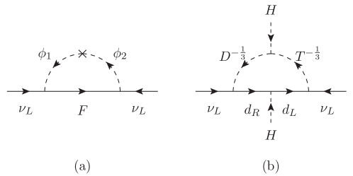
Figure 1: The Feynman diagrams for the neutrino mass generation. (a) General case, where $\phi_{1,2}$ are in their interaction basis, and $F$ is in its mass eigenstate, and (b) for this model, where the fields are in the interaction basis. Here all the flavor indices are omitted.

Instead of using the bi-lepton $SU(2)$ singlet and a charged scalar without lepton number as first proposed in Ref.[107], we employ two leptoquarks which carry different lepton numbers to break the lepton number and generate the neutrino mass radiactively. We start with a general discussion on the 1-loop neutrino mass generation. If there are two scalars $\phi_{1,2}$ which interact with fermion $F_{k}$ and the neutrino via a general Yukawa coupling parameterized as

$${\cal L}\supset\lambda_{ij}\bar{F}_{j}\nu_{Li}\phi_{1}+\kappa_{ij}\bar{F}_{j}\nu^{c}_{i}\phi_{2}+H.c.\,,$$ (24)

where the fermion $F$ can carry arbitrary lepton number and baryon number $(L_{F},B_{F})$. If the two scalars do not mix, $\phi_{1}/\phi_{2}$ can be assigned with the lepton-number and baryon number $(L_{F}-1,L_{B})/(L_{F}+1,L_{B})$ and the Lagrangian enjoys both the global lepton-number $U(1)_{L}$ and the global baryon-number $U(1)_{B}$ symmetries. Without losing the generality, $F_{k}$ is assumed to be in its mass eigenstate with a mass $m_{k}$. If $\phi_{1,2}$ can mix with each other, the lepton number is broken by two units, and the Weinberg operator[113] can be generated radiatively. Let’s denote $\phi_{h(l)}$ as the heavier(lighter) mass state with mass $m_{h}(m_{l})$, and parameterize their mixing as $\phi_{1}=c_{\alpha}\phi_{l}+s_{\alpha}\phi_{h}$ and $\phi_{2}=-s_{\alpha}\phi_{l}+c_{\alpha}\phi_{h}$, where $s_{\alpha}(c_{\alpha})$ is the shorthand notation for $\sin\alpha(\cos\alpha)$ and $\alpha$ is the mixing angle. The resultant neutrino mass from Fig.1(a) can be calculated as

$$M^{\nu}_{ij}=\sum_{k}{N^{F}_{c}m_{k}\over 16\pi^{2}}s_{\alpha}c_{\alpha}(\kappa_{ik}\lambda_{jk}+\kappa_{jk}\lambda_{ik})\left[{m_{h}^{2}\over m_{h}^{2}-m_{k}^{2}}\ln\frac{m_{h}^{2}}{m_{k}^{2}}-{m_{l}^{2}\over m_{l}^{2}-m_{k}^{2}}\ln\frac{m_{l}^{2}}{m_{k}^{2}}\right]\,,$$ (25)

which is exact and free of divergence. Note that for the diagonal element, the combination in the bracket should be replaced by $2\mbox{Re}(\kappa_{ik}\lambda_{ik})$. When the mixing is small, this result can also be approximately calculated in the interaction basis of $\phi_{1}$ and $\phi_{2}$.

In our model, the mass eigenstate $F$ can be the SM down-type quark or the exotic $b^{\prime}$, and $D^{\frac{1}{3}}/T^{\frac{1}{3}}$ plays the role of $\phi_{1}/\phi_{2}$, as depicted in Fig.1(b). Assume the $D\mathchar 45\relax T$ mixing is small, then

$$M^{\nu}_{ij}\simeq\sum_{k=d,s,b,b^{\prime}}{3m_{k}\over 32\pi^{2}}(\lambda^{T}_{ik}\lambda^{D}_{jk}+\lambda^{T}_{jk}\lambda^{D}_{ik}){\mu_{3}v_{0}\over M_{D}^{2}-M_{T}^{2}}\ln\frac{M_{T}^{2}}{M_{D}^{2}}$$ (26)

for $i\neq j$, and $2\mbox{Re}(\lambda^{T}_{ik}\lambda^{D}_{ik})$ should be used in the bracket for the diagonal elements. To have sub-eV neutrino masses, we need roughly

$$\mu_{3}m_{b}\lambda^{D}\lambda^{T}\,,\,\mu_{3}M_{b^{\prime}}\lambda^{D}\lambda^{T}\simeq{\cal O}(10^{-5})\times\left(\frac{M_{LQ}}{\mbox{TeV}}\right)^{2}(\mathrm{GeV})^{2}$$ (27)

if $b^{(^{\prime})}$-quark contribution dominates. More comprehensive numerical consideration with other phenomenology will be given in section IV.

III.2 $(g-2)$ of charged leptons

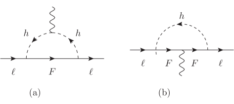
Figure 2: The Feynman diagrams in the mass basis for the anomalous magnetic dipole moment of charged lepton in general cases.

We also start with a general discussion on the 1-loop contribution to $(g-2)_{\ell}$ by adding a fermion, $F$, and a charged scalar, $h$. The $F\mathchar 45\relax\ell\mathchar 45\relax h$ Yukawa interaction can be parameterized as

$${\cal L}\supset\bar{F}(y^{l}_{R}\hat{R}+y^{l}_{L}\hat{L})\ell h+H.c.$$ (28)

where both $F$ and $\ell$ are in their mass eigenstates. Here, we have suppressed the flavor indices but it should be understood that both $y_{R}$ and $y_{L}$ are in general flavor dependent. Then, the resulting 1-loop anomalous magnetic moment depicted in Fig.2(a,b) can be calculated as

$$\triangle a^{h}_{l} = \frac{-N^{F}_{c}(1+Q_{F})m_{l}^{2}}{8\pi^{2}}\int^{1}_{0}dx\,x(1-x){x\frac{|y^{l}_{L}|^{2}+|y^{l}_{R}|^{2}}{2}+\frac{m_{F}}{m_{l}}\Re[(y^{l}_{R})^{*}y^{l}_{L}]\over x^{2}m_{l}^{2}+x(m_{h}^{2}-m_{l}^{2})+(1-x)m_{F}^{2}}\,,$$ (29)

$$\triangle a^{F}_{l} = \frac{-N^{F}_{c}Q_{F}m_{l}^{2}}{8\pi^{2}}\int^{1}_{0}dx\,x^{2}{(1-x)\frac{|y^{l}_{L}|^{2}+|y^{l}_{R}|^{2}}{2}+\frac{m_{F}}{m_{l}}\Re[(y^{l}_{R})^{*}y^{l}_{L}]\over x^{2}m_{l}^{2}+x(m_{F}^{2}-m_{l}^{2})+(1-x)m_{h}^{2}}\,,$$ (30)

where $Q_{F}$ is the electric charge of $F$, and $\triangle a_{l}^{F}(\triangle a_{l}^{h})$ is the contribution with the external photon attached to the fermion (scalar) inside the loop. We keep $\triangle a_{l}^{F}(\triangle a_{l}^{h})$ in the integral form since the analytic expression of resulting integration is not illuminating at all. The physics is also clear from the above expression that one needs $m_{F}\gg m_{l}$ also both $y^{l}_{R}$ and $y^{l}_{L}$ nonzero to make $\triangle a_{e}$ and $\triangle a_{\mu}$ of opposite sign. For $m_{F}\gg m_{l}$, we have

$$\triangle a_{l}^{h} \simeq \Re[(y^{l}_{R})^{*}y^{l}_{L}]\left(\frac{m_{l}}{m_{F}}\right)\frac{-N^{F}_{c}(1+Q_{F})}{8\pi^{2}}\int^{1}_{0}dx\,{x(1-x)\over x+(1-x)\frac{m_{h}^{2}}{m_{F}^{2}}}\,,$$ (31)

$$\triangle a_{l}^{F} \simeq \Re[(y^{l}_{R})^{*}y_{L}]\left(\frac{m_{l}}{m_{F}}\right)\frac{-N^{F}_{c}Q_{F}}{8\pi^{2}}\int^{1}_{0}dx\,{x^{2}\over x+(1-x)\frac{m_{h}^{2}}{m_{F}^{2}}}\,.$$ (32)

Namely,

$$\triangle a_{l}=\triangle a_{l}^{F}+\triangle a_{l}^{h}\simeq-\frac{N^{F}_{c}\Re[(y^{l}_{R})^{*}y_{L}]}{8\pi^{2}}\left(\frac{m_{l}}{m_{F}}\right){\cal J}_{Q_{F}}\left(\frac{m_{h}^{2}}{m_{F}^{2}}\right)\,,$$ (33)

where

$${\cal J}_{Q}(\alpha) = \int^{1}_{0}dx\,{x(1-x)+x\,Q\over x+(1-x)\alpha}$$ (34)

$$= {2Q(1-\alpha)(1-\alpha+\alpha\ln\alpha)+(1-\alpha^{2}+2\alpha\ln\alpha)\over 2(1-\alpha)^{3}}\,.$$

From Eq.(34), it is clear that ${\cal J}_{Q}(0)=(1+2Q)/2$, ${\cal J}_{Q}(1)=(1+3Q)/6$, and ${\cal J}_{Q}(\alpha)\rightarrow(Q\ln\alpha-1/2)/\alpha$ for $\alpha\gg 1$.

Similar calculation leads to a $l\rightarrow l^{\prime}\gamma$ transition amplitude:

$$i{\cal M}\simeq ie\frac{m_{l}N_{c}^{F}}{16\pi^{2}m_{F}}{\cal J}_{Q_{F}}(\beta_{h})\times\overline{u_{l^{\prime}}}(p-k)\left[\frac{i\sigma^{\alpha\beta}k_{\beta}\epsilon^{*}_{\alpha}}{m_{l}}\left(A^{ll^{\prime}}_{M}+A^{ll^{\prime}}_{E}\gamma^{5}\right)\right]u_{l}(p)\,,$$ (35)

where $\beta_{h}=(m_{h}/m_{F})^{2}$, $\epsilon$ is the polarization of the photon, and

$$A^{ll^{\prime}}_{M}=\frac{1}{2}\left[(y^{l^{\prime}}_{R})^{*}y^{l}_{L}+(y^{l^{\prime}}_{L})^{*}y^{l}_{R}\right]\,,\;A^{ll^{\prime}}_{E}=\frac{1}{2}\left[(y^{l^{\prime}}_{R})^{*}y^{l}_{L}-(y^{l^{\prime}}_{L})^{*}y^{l}_{R}\right]\,.$$ (36)

For $l=\mu$ and $l^{\prime}=e$, the above transition amplitude results in the $\mu\rightarrow e\gamma$ branching ratio[114]

$$Br(\mu\rightarrow e\gamma)={3\alpha(N^{F}_{c})^{2}\over 8\pi G_{F}^{2}m_{F}^{2}m_{\mu}^{2}}\left(\left|A^{\mu e}_{M}\right|^{2}+\left|A^{\mu e}_{E}\right|^{2}\right)\,,$$ (37)

and it must complies with the current experimental limit, $Br(\mu\rightarrow e\gamma)<4.2\times 10^{-13}$[115], or $|A^{\mu e}_{E,M}|\lesssim{\cal O}(10^{-8})$. Moreover, if the dipole transition is dominate, then

$${Br(\mu\rightarrow 3e)\over Br(\mu\rightarrow e\gamma)}=\frac{2\alpha}{3\pi}\left[\ln\frac{m_{\mu}}{m_{e}}-\frac{11}{8}\right]\simeq 6.12\times 10^{-3}\,,$$ (38)

thus can be ignored.

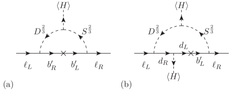
Figure 3: The Feynman diagrams, in the interaction basis, for the anomalous magnetic dipole moment of charged lepton in this model. Here all the flavor indices are omitted. The external photon (not shown ) can be attached to any charged particle in the loop.

In our model, the vector fermion $b^{\prime}_{L,R}(3,1,-1/3)$, Fig.3(a), and/or the SM b-quark, Fig.3(b), can play the role of $F$ both carrying an electric charge $-\frac{1}{3}$. The function ${\cal J}_{-\frac{1}{3}}(\alpha)$ takes a value in the range from $-0.022$ to $0.087$ for $\alpha\in[0.1,10.0]$. In the interaction basis, $T(3,3,-1/3)$ does not couple to $b^{\prime}$, $D(3,2,1/6)$ only couples to left-handed charged lepton, and $S(3,1,2/3)$ only couples to the right-handed charged lepton. Due to the $D\mathchar 45\relax S$ and $D\mathchar 45\relax T$ mixings, the three charge-$2/3$ physical mass states acquire both the LH and RH Yukawa couplings as shown in Eq.(28). However, the physical state dominated by the $T$ component gets double suppression form $D\mathchar 45\relax T$ and $d\mathchar 45\relax b^{\prime}$ mixings, thus not important here. Assuming small $D\mathchar 45\relax S$ mixing in our model, the anomalous magnetic moment of charged lepton becomes

$$\triangle a_{l} \simeq (\lambda^{D}_{lb^{\prime}}\lambda^{S}_{lb^{\prime}}){3\mu_{1}v_{0}\over 16\sqrt{2}\pi^{2}}\frac{m_{l}}{M^{3}_{b^{\prime}}}\times{\cal K}\left(\frac{M_{D}^{2}}{M^{2}_{b^{\prime}}},\frac{M_{S}^{2}}{M^{2}_{b^{\prime}}}\right)$$ (39)

$$+ (\lambda^{D}_{lb}\lambda^{S}_{lb}){3\mu_{1}v_{0}\over 16\sqrt{2}\pi^{2}}\frac{m_{l}}{m^{3}_{b}}\times{\cal K}\left(\frac{M_{D}^{2}}{m^{2}_{b}},\frac{M_{S}^{2}}{m^{2}_{b}}\right)\,,$$

where

$${\cal K}(a,b)\equiv{{\cal J}_{-\frac{1}{3}}(a)-{\cal J}_{-\frac{1}{3}}(b)\over b-a}\,.$$ (40)

When $a\simeq b$, the function ${\cal K}$ takes a limit

$${\cal K}(a,b)\stackrel{{\scriptstyle b\rightarrow a}}{{\Rightarrow}}-\left.\frac{d}{d\alpha}{\cal J}_{-\frac{1}{3}}(\alpha)\right|_{\alpha=a}=-{11-4a-7a^{2}+2[2+a(6+a)]\ln a\over 6(1-a)^{4}}\,.$$ (41)

For $a\simeq b\simeq 1$, it can be approximated by ${\cal K}(a,b)\simeq 1/36-(a+b-2)/45$, and ${\cal K}(a,b)\simeq-\ln a/(3a^{2})$ for $a\simeq b\gg 1$.

If factoring out the $M_{F}=M_{b^{\prime}}$, the dipole transition coefficients in Eq.(37) are given by

$$A^{\mu e}_{M/E}\simeq-{\mu_{1}v_{0}\over 4\sqrt{2}M_{b^{\prime}}^{2}}\left\{\left[(\lambda^{S}_{eb^{\prime}})^{*}\lambda^{D}_{\mu b^{\prime}}\pm(\lambda^{D}_{eb^{\prime}})^{*}\lambda^{S}_{\mu b^{\prime}}\right]{\cal K}(\beta_{D},\beta_{S})+\frac{M_{b^{\prime}}^{3}}{m_{b}^{3}}\left[(\lambda^{S}_{eb})^{*}\lambda^{D}_{\mu b}\pm(\lambda^{D}_{eb})^{*}\lambda^{S}_{\mu b}\right]{\cal K}(b_{D},b_{S})\right\}\,,$$ (42)

where $b_{D,S}\equiv(M_{D,S}/m_{b})^{2}$, and $\beta_{D,S}=(M_{D,S}/M_{b^{\prime}})^{2}$. The current upper bound of $Br(\mu\rightarrow e\gamma)$ amounts to a stringent limit that the relevant $|\lambda^{S}\lambda^{D}|\lesssim 10^{-5}$. Instead of making the product of Yukawa couplings small, the $\mu\rightarrow e\gamma$ transition from $D\mathchar 45\relax S$ mixing, Fig.3, can be simply arranged to vanish if muon/electron only couples to $b^{\prime}/b$ or the other way around.

Modulating by the leptoquark masses, numerically we have either

Sol-1 $$:$$

$$\triangle a_{e} \simeq 2.28\times 10^{-5}\times[\lambda^{D}_{eb}\lambda^{S}_{eb}]\times\left(\frac{\mu_{1}}{\mbox{GeV}}\right)\times{\cal K}(b_{D},b_{S})\,,$$

$$\triangle a_{\mu} \simeq 1.03\times 10^{-10}\times[\lambda^{D}_{\mu b^{\prime}}\lambda^{S}_{\mu b^{\prime}}]\times\left(\frac{\mu_{1}}{\mbox{GeV}}\right)\left(\frac{1.5\mathrm{TeV}}{M_{b^{\prime}}}\right)^{3}\times{\cal K}(\beta_{D},\beta_{S})\,,$$ (43)

or

Sol-2 $$:$$

$$\triangle a_{e} \simeq 5.00\times 10^{-13}\times[\lambda^{D}_{eb^{\prime}}\lambda^{S}_{eb^{\prime}}]\times\left(\frac{\mu_{1}}{\mbox{GeV}}\right)\left(\frac{1.5\mathrm{TeV}}{M_{b^{\prime}}}\right)^{3}\times{\cal K}(\beta_{D},\beta_{S})\,,$$

$$\triangle a_{\mu} \simeq 4.71\times 10^{-3}\times[\lambda^{D}_{\mu b}\lambda^{S}_{\mu b}]\times\left(\frac{\mu_{1}}{\mbox{GeV}}\right)\times{\cal K}(b_{D},b_{S})\,.$$ (44)

For $M_{b^{\prime}}=1.5\mathrm{TeV}$ and $M_{LQ}\simeq 1\mathrm{TeV}$, then either $\left\{\mu_{1}\lambda^{D}_{eb}\lambda^{S}_{eb}\,,\;\mu_{1}\lambda^{D}_{\mu b^{\prime}}\lambda^{S}_{\mu b^{\prime}}\right\}\simeq\{49.4[-27.3],279.9\}\mathrm{GeV}$ for (Sol-1), or $\left\{\mu_{1}\lambda^{D}_{eb^{\prime}}\lambda^{S}_{eb^{\prime}}\,,\;\mu_{1}\lambda^{D}_{\mu b}\lambda^{S}_{\mu b}\right\}\simeq\{-20.1[11.1],-689.5\}\mbox{GeV}$ for (Sol-2) can accommodate the observed central values of $\triangle a_{e}^{Cs}[\triangle a_{e}^{Rb}]$ and $\triangle a_{\mu}$ simultaneously with vanishing $Br(\mu\rightarrow e\gamma)$. However, as will be discussed later, only Sol-2 is viable to simultaneously accommodate the neutrino data.

III.3 $b\rightarrow sl^{+}l^{-}$

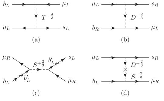
Figure 4: The potential tree-level Feynman diagrams for $b\rightarrow s\mu\bar{\mu}$ transition.

The $b\rightarrow s\mu\bar{\mu}$ transition can be generated by tree-level diagrams mediated by $T^{\frac{4}{3}}$, $D^{\frac{2}{3}}$, $S^{\frac{2}{3}}$, and the one from $D\mathchar 45\relax S$ mixing, see Fig.4. In Fig.4(c), the crosses represent the mixing between the $b^{\prime}_{L}$ and the physical $b$ and $s$ quarks, because $S$ only couples to $b^{\prime}_{L}$ in the interaction basis. From Eq.(139), we see that this model can yield $b\rightarrow s\mu\bar{\mu}$ operators in the vector, scalar, and tensor forms. However, we failed to find a viable parameter space to explain the $b\rightarrow sl^{+}l^{-}$ anomaly and simultaneously comply with other experimental constraints, see Sec.IV.1.

Instead, to bypass the stringent experimental bounds and the fine-tuning of the parameters, we go for the 1-loop box diagram contribution, as shown in Fig.5, which requires only four nonzero triplet Yukawa couplings $\lambda^{T}_{\tau s},\lambda^{T}_{\tau b},\lambda^{T}_{\mu b},\lambda^{T}_{\mu b^{\prime}}$.

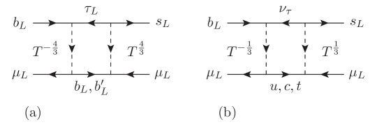
Figure 5: The Feynman diagram for $b\rightarrow s\mu\bar{\mu}$ transition.

In the usual convention, the transition is described by a low energy effective Hamiltonian

$${\cal H}^{b\rightarrow s\mu\mu}_{eff}=-\frac{G_{F}}{\sqrt{2}}\widetilde{V}_{tb}\widetilde{V}_{ts}^{*}\frac{\alpha}{\pi}\sum_{i}{\cal C}_{i}{\cal O}_{i}+H.c.$$ (45)

with

$${\cal O}_{9}=\left(\bar{s}\gamma^{\alpha}\hat{L}b\right)\left(\bar{\mu}\gamma_{\alpha}\mu\right)\,,\,\,{\cal O}_{10}=\left(\bar{s}\gamma^{\alpha}\hat{L}b\right)\left(\bar{\mu}\gamma_{\alpha}\gamma^{5}\mu\right)\,,$$ (46)

$${\cal O}^{\prime}_{9}=\left(\bar{s}\gamma^{\alpha}\hat{R}b\right)\left(\bar{\mu}\gamma_{\alpha}\mu\right)\,,\,\,{\cal O}^{\prime}_{10}=\left(\bar{s}\gamma^{\alpha}\hat{R}b\right)\left(\bar{\mu}\gamma_{\alpha}\gamma^{5}\mu\right)\,.$$ (47)

Ignoring the tau mass in the loop, Fig.5(a), the effective Hamiltonian generated by the box-diagram can be easily calculated as

$${\cal H}^{b\rightarrow s\mu\mu}_{eff(a)}\simeq-{\lambda^{T}_{\tau b}(\lambda^{T}_{\tau s})^{*}\over 64\pi^{2}}\left(\frac{|\lambda^{T}_{\mu b^{\prime}}|^{2}}{M_{b^{\prime}}^{2}}{\cal G}(\beta^{\prime}_{T})+\frac{|\lambda^{T}_{\mu b}|^{2}}{m_{b}^{2}}{\cal G}(\beta_{T})\right)\left(\bar{s}\gamma^{\alpha}\hat{L}b\right)\left(\bar{\mu}\gamma_{\alpha}\hat{L}\mu\right)+H.c.\,,$$ (48)

where $\beta^{\prime}_{T}\equiv(M_{T}/M_{b^{\prime}})^{2}$, $\beta_{T}\equiv(M_{T}/m_{b})^{2}$, and

$${\cal G}(x)=\left[\frac{1}{1-x}+\frac{\ln x}{(1-x)^{2}}\right]\,.$$ (49)

The function has a limit ${\cal G}(x=1)=-1/2$, and ${\cal G}\rightarrow-1/x$ when $x\gg 1$.

The second contribution from the box diagram with $T^{\pm\frac{1}{3}}$ and up-type quark running in the loop yields

$${\cal H}^{b\rightarrow s\mu\mu}_{eff(b)}\simeq{\lambda^{T}_{\tau b}(\lambda^{T}_{\tau s})^{*}\over 64\pi^{2}}\frac{1}{4M_{T}^{2}}\left[|\lambda^{T}_{\mu b^{\prime}}|^{2}(s_{1}^{2}+s_{2}^{2}+s_{3}^{2})+|\lambda^{T}_{\mu b}|^{2}\right]\left(\bar{s}\gamma^{\alpha}\hat{L}b\right)\left(\bar{\mu}\gamma_{\alpha}\hat{L}\mu\right)+H.c.\,.$$ (50)

In arriving the above expression, we have made use of the unitarity of $\widetilde{V}$, namely,

$$|\widetilde{V}_{ub^{\prime}}|^{2}+|\widetilde{V}_{cb^{\prime}}|^{2}+|\widetilde{V}_{tb^{\prime}}|^{2}=1-c_{1}^{2}c_{2}^{2}c_{3}^{2}\simeq s_{1}^{2}+s_{2}^{2}+s_{3}^{2}\ll 1\,,$$ (51)

and

$$|\widetilde{V}_{ub}|^{2}+|\widetilde{V}_{cb}|^{2}+|\widetilde{V}_{tb}|^{2}\simeq 1\,.$$ (52)

It is clear that the contribution from Fig.5(b) is dominated by $\lambda^{T}_{\mu b}$.

And the relevant Wilson coefficients are determined to be

$${\cal C}_{9} = -{\cal C}_{10}\simeq\frac{\sqrt{2}}{128\pi\alpha}{\lambda^{T}_{\tau b}(\lambda^{T}_{\tau s})^{*}\over V_{tb}V_{ts}^{*}G_{F}M_{T}^{2}}\left[|\lambda^{T}_{\mu b^{\prime}}|^{2}\beta^{\prime}_{T}{\cal G}(\beta^{\prime}_{T})-\frac{5}{4}|\lambda^{T}_{\mu b}|^{2}\right]\,,$$

$${\cal C}^{\prime}_{9} = -{\cal C}^{\prime}_{10}=0\,.$$ (53)

For a typical value of $\beta^{\prime}_{T}=(1.0\mbox{TeV}/1.5\mbox{TeV})^{2}$, $\beta^{\prime}_{T}{\cal G}(\beta^{\prime}_{T})=-0.3677$.

We use the following values,

$$({\cal C}_{9})^{\mu}=-({\cal C}_{10})^{\mu}\simeq-0.41\pm 0.07\,,$$ (54)

for muon, and

$$({\cal C}_{9})^{e}\simeq({\cal C}_{10})^{e}\simeq({\cal C}^{\prime}_{9})^{e}\simeq({\cal C}^{\prime}_{10})^{e}\simeq 0$$ (55)

for the electron counter part, from the global fit to the $b\rightarrow sl^{+}l^{-}$ data [63] .

If we take $\widetilde{V}_{tb}\widetilde{V}_{ts}^{*}=-0.03975$, then it amounts to

$$\lambda^{T}_{\tau b}(\lambda^{T}_{\tau s})^{*}\left[-|\lambda^{T}_{\mu b^{\prime}}|^{2}\beta^{\prime}_{T}{\cal G}(\beta^{\prime}_{T})+\frac{5}{4}|\lambda^{T}_{\mu b}|^{2}\right]\simeq-(0.394\pm 0.067)\left(\frac{M_{T}}{\mbox{TeV}}\right)^{2}\,.$$ (56)

Since the combination in the squared bracket is positive, the product $\lambda^{T}_{\tau b}(\lambda^{T}_{\tau s})^{*}$ has to be negative. The constraints from $B_{s}\mathchar 45\relax\overline{B}_{s}$ mixing and $b\rightarrow s\gamma$ will be carefully discussed in Sec.IV.

III.4 Cabibbo-angle anomaly

From the unitarity of $\widetilde{V}_{4}$, it is clear that

$$|\widetilde{V}_{ud}|^{2}+|\widetilde{V}_{us}|^{2}+|\widetilde{V}_{ub}|^{2}=1-|\widetilde{V}_{ub^{\prime}}|^{2}\leq 1\,,$$ (57)

and the Cabibbo-angle anomaly(CAA) is naturally embedded in this model. Moreover, the most commonly discussed unitarity triangle becomes

$$\widetilde{V}_{ud}\widetilde{V}_{ub}^{*}+\widetilde{V}_{cd}\widetilde{V}_{cb}^{*}+\widetilde{V}_{td}\widetilde{V}_{tb}^{*}=-(U^{d}_{L})_{d4}^{*}(U^{d}_{L})_{b4}\,.$$ (58)

Similarly, this model also predicts that

$$|\widetilde{V}_{cd}|^{2}+|\widetilde{V}_{cs}|^{2}+|\widetilde{V}_{cb}|^{2}=1-|\widetilde{V}_{cb^{\prime}}|^{2}\,,$$ (59)

$$|\widetilde{V}_{td}|^{2}+|\widetilde{V}_{ts}|^{2}+|\widetilde{V}_{tb}|^{2}=1-|\widetilde{V}_{tb^{\prime}}|^{2}\,,$$ (60)

$$|\widetilde{V}_{ud}|^{2}+|\widetilde{V}_{cd}|^{2}+|\widetilde{V}_{td}|^{2}=1-|(U^{d}_{L})_{d4}|^{2}\,,$$ (61)

$$|\widetilde{V}_{us}|^{2}+|\widetilde{V}_{cs}|^{2}+|\widetilde{V}_{ts}|^{2}=1-|(U^{d}_{L})_{s4}|^{2}\,,$$ (62)

$$|\widetilde{V}_{ub}|^{2}+|\widetilde{V}_{cb}|^{2}+|\widetilde{V}_{tb}|^{2}=1-|(U^{d}_{L})_{b4}|^{2}\,,$$ (63)

and all the other SM CKM unitary triangles are no more closed in general.

The matrix elements are easy to read. For example, we have

$$\widetilde{V}_{us}=c_{2}V_{us}-s_{2}s_{3}V_{ub}\,,\;\widetilde{V}_{ub^{\prime}}=s_{1}V_{ud}+c_{1}s_{2}V_{us}+c_{1}c_{2}s_{3}V_{ub}\,,$$ (64)

$$\left\{(U^{d}_{L})_{d4},(U^{d}_{L})_{s4},(U^{d}_{L})_{b4},(U^{d}_{L})_{b^{\prime}4}\right\}=\left\{-s_{1}c_{2}c_{3},-s_{2}c_{3},-s_{3},c_{1}c_{2}c_{3}\right\}\,.$$ (65)

The mixing $\theta_{i}$ is expected to be small, so a smaller universal

$$\left|\widetilde{V}_{us}\right|\simeq\left|V_{us}\right|\left(1-\frac{\theta_{2}^{2}}{2}\right)$$ (66)

to leading order is expected as well. By using the Wolfenstein parameterization and the central values from global fit[1], we have

$$\widetilde{V}_{ub^{\prime}}\simeq 0.9740s_{1}+0.2265c_{1}s_{2}+0.0036c_{1}c_{2}s_{3}e^{1.196i}\,.$$ (67)

Therefore, to accommodate the deficit of 1st row CKM unitarity (Eq.(6) and Eq.(57)) we have

$$\left|s_{1}+0.233s_{2}\right|\simeq 0.039(7)\,.$$ (68)

IV Constraints and parameter space

As discussed in the previous section, this model is capable to address neutrino mass generation, $\triangle a_{e,\mu}$, $b\rightarrow s\mu\mu$, and the CAA. For readers’ convenience, all the requirements are collected and displayed in Table 4.

Anomaly	Requirement	Remark
$m_{\nu}$	$\mu_{3}m_{b^{(^{\prime})}}\lambda^{D}\lambda^{T}\simeq{\cal O}(10^{-5})(\mathrm{GeV})^{2}$	Eq.(26)
$\triangle a_{e}^{Cs[Rb]},\triangle a_{\mu}$ ( Sol-1 )	$\left\{\mu_{1}\lambda^{D}_{eb}\lambda^{S}_{eb}\,,\;\mu_{1}\lambda^{D}_{\mu b^{\prime}}\lambda^{S}_{\mu b^{\prime}}\right\}\simeq\{(49\pm 20)[-27\pm 17],(280\pm 66)\}\mbox{GeV}$	Eq.(43)
$\triangle a_{e}^{Cs[Rb]},\triangle a_{\mu}$ ( Sol-2 )	$\left\{\mu_{1}\lambda^{D}_{eb^{\prime}}\lambda^{S}_{eb^{\prime}}\,,\;\mu_{1}\lambda^{D}_{\mu b}\lambda^{S}_{\mu b}\right\}\simeq\{-(20.1\pm 8.3)[+11.1\pm 6.9],-(689\pm 162)\}\mbox{GeV}$	Eq.(44)
$b\rightarrow sl^{+}l^{-}$	$\lambda^{T}_{\tau b}(\lambda^{T}_{\tau s})^{*}(|\lambda^{T}_{\mu b^{\prime}}|^{2}+3.39|\lambda^{T}_{\mu b}|^{2})\simeq-(1.07\pm 0.18)$	Eq.(53)
Cabibbo angle anomaly	$\left|s_{1}+0.233s_{2}\right|\simeq 0.039(7)$	Eq.(57)

Table 4: The requirement for explaining each mechanism/anomaly. For illustration, we take the following values: $\widetilde{V}_{tb}\widetilde{V}_{ts}^{*}=-0.03975$, $M_{LQ}=1.0$ TeV, and $M_{b^{\prime}}=1.5$ TeV.

In this section, we should carefully scrutinize all the existing experimental limits and try to identify the viable model parameter at the end.

IV.1 Low energy $2q2l$ effective Hamiltonian

${(\bar{q}_{k}\gamma^{\mu}\hat{L}q_{l})(\bar{e}_{i}\gamma_{\mu}\hat{L}e_{j})\over 4M_{T}^{2}}$	Wilson Coef.	Constraint	Model
$bb\mu\mu$	$2|\lambda^{T}_{\mu b}|^{2}$	$211.1$[116]	$1.06$
$sb\tau\tau$	$2\lambda^{T}_{\tau b}(\lambda^{T}_{\tau s})^{*}$	-	$-0.14$
$sb\mu\mu$	$0$	-	$0$
$sb\mu\tau$	$0$	-	$0$
$sb\tau\mu$	$2\lambda^{T}_{\mu b}(\lambda^{T}_{\tau s})^{*}$	$0.199$[116]	$0.11$
$uu\tau\mu$	$\left(\widetilde{V}_{ub}(\lambda^{T}_{\tau b})^{*}+\widetilde{V}_{ub^{\prime}}(\lambda^{T}_{\tau b^{\prime}})^{*}+\widetilde{V}_{us}(\lambda^{T}_{\tau s})^{*}\right)\times\left(\widetilde{V}^{*}_{ub}\lambda^{T}_{\mu b}+\widetilde{V}^{*}_{ub^{\prime}}\lambda^{T}_{\mu b^{\prime}}\right]$	$0.13$[116]	$0.0043$
$uu\mu\mu$	$\left|\widetilde{V}_{ub}(\lambda^{T}_{\mu b})^{*}+\widetilde{V}_{ub^{\prime}}(\lambda^{T}_{\mu b^{\prime}})^{*}\right|^{2}$	$1.03$[116]	$0.017$
$uc\mu\mu$	$\left(\widetilde{V}_{ub}(\lambda^{T}_{\mu b})^{*}+\widetilde{V}_{ub^{\prime}}(\lambda^{T}_{\mu b^{\prime}})^{*}\right)\times\left(\widetilde{V}^{*}_{cb}\lambda^{T}_{\mu b}+\widetilde{V}^{*}_{cb^{\prime}}\lambda^{T}_{\mu b^{\prime}}\right)$	$0.11$[116]	$0^{*}$
$cc\mu\mu$	$\left|\widetilde{V}_{cb}(\lambda^{T}_{\mu b})^{*}+\widetilde{V}_{cb^{\prime}}(\lambda^{T}_{\mu b^{\prime}})^{*}\right|^{2}$	$52.8$[116]	$0^{*}$
$cc\tau\mu$	$\left(\widetilde{V}_{cb}(\lambda^{T}_{\tau b})^{*}+\widetilde{V}_{cb^{\prime}}(\lambda^{T}_{\tau b^{\prime}})^{*}+\widetilde{V}_{cs}(\lambda^{T}_{\tau s})^{*}\right)\times\left(\widetilde{V}^{*}_{cb}\lambda^{T}_{\mu b}+\widetilde{V}^{*}_{cb^{\prime}}\lambda^{T}_{\mu b^{\prime}}\right)$	$211.1$[116]	$0^{*}$
$tc\mu\mu$	$\left(\widetilde{V}_{tb}(\lambda^{T}_{\mu b})^{*}+\widetilde{V}_{tb^{\prime}}(\lambda^{T}_{\mu b^{\prime}})^{*}\right)\times\left(\widetilde{V}^{*}_{cb}\lambda^{T}_{\mu b}+\widetilde{V}^{*}_{cb^{\prime}}\lambda^{T}_{\mu b^{\prime}}\right)$	-	$0^{*}$
$tc\tau\tau$	$\left(\widetilde{V}_{tb}(\lambda^{T}_{\tau b})^{*}+\widetilde{V}_{tb^{\prime}}(\lambda^{T}_{\tau b^{\prime}})^{*}+\widetilde{V}_{ts}(\lambda^{T}_{\tau s})^{*}\right)\times\left(\widetilde{V}^{*}_{cb}\lambda^{T}_{\tau b}+\widetilde{V}^{*}_{cb^{\prime}}\lambda^{T}_{\tau b^{\prime}}+\widetilde{V}^{*}_{cs}\lambda^{T}_{\tau s}\right)$	-	$-0.030$
$tc\tau\mu$	$\left(\widetilde{V}_{tb}(\lambda^{T}_{\tau b})^{*}+\widetilde{V}_{tb^{\prime}}(\lambda^{T}_{\tau b^{\prime}})^{*}+\widetilde{V}_{ts}(\lambda^{T}_{\tau s})^{*}\right)\times\left(\widetilde{V}^{*}_{cb}\lambda^{T}_{\mu b}+\widetilde{V}^{*}_{cb^{\prime}}\lambda^{T}_{\mu b^{\prime}}\right)$	$11.35$	$0^{*}$
$tc\mu\tau$	$\left(\widetilde{V}_{tb}(\lambda^{T}_{\mu b})^{*}+\widetilde{V}_{tb^{\prime}}(\lambda^{T}_{\mu b^{\prime}})^{*}\right)\times\left(\widetilde{V}^{*}_{cb}\lambda^{T}_{\tau b}+\widetilde{V}^{*}_{cb^{\prime}}\lambda^{T}_{\tau b^{\prime}}+\widetilde{V}^{*}_{cs}\lambda^{T}_{\tau s}\right)$	$11.35$	$0.02$
$tu\mu\mu$	$\left(\widetilde{V}_{tb}(\lambda^{T}_{\mu b})^{*}+\widetilde{V}_{tb^{\prime}}(\lambda^{T}_{\mu b^{\prime}})^{*}\right)\times\left(\widetilde{V}^{*}_{ub}\lambda^{T}_{\mu b}+\widetilde{V}^{*}_{ub^{\prime}}\lambda^{T}_{\mu b^{\prime}}\right)$	-	$0.09$
$tu\tau\tau$	$\left(\widetilde{V}_{tb}(\lambda^{T}_{\tau b})^{*}+\widetilde{V}_{tb^{\prime}}(\lambda^{T}_{\tau b^{\prime}})^{*}+\widetilde{V}_{ts}(\lambda^{T}_{\tau s})^{*}\right)\times\left(\widetilde{V}^{*}_{ub}\lambda^{T}_{\tau b}+\widetilde{V}^{*}_{ub^{\prime}}\lambda^{T}_{\tau b^{\prime}}+\widetilde{V}^{*}_{us}\lambda^{T}_{\tau s}\right)$	-	$-0.03$
$tu\tau\mu$	$\left(\widetilde{V}_{tb}(\lambda^{T}_{\tau b})^{*}+\widetilde{V}_{tb^{\prime}}(\lambda^{T}_{\tau b^{\prime}})^{*}+\widetilde{V}_{ts}(\lambda^{T}_{\tau s})^{*}\right)\times\left(\widetilde{V}^{*}_{ub}\lambda^{T}_{\mu b}+\widetilde{V}^{*}_{ub^{\prime}}\lambda^{T}_{\mu b^{\prime}}\right)$	$11.35$	$-0.12$
$tu\mu\tau$	$\left(\widetilde{V}_{tb}(\lambda^{T}_{\mu b})^{*}+\widetilde{V}_{tb^{\prime}}(\lambda^{T}_{\mu b^{\prime}})^{*}\right)\times\left(\widetilde{V}^{*}_{ub}\lambda^{T}_{\tau b}+\widetilde{V}^{*}_{ub^{\prime}}\lambda^{T}_{\tau b^{\prime}}+\widetilde{V}^{*}_{us}\lambda^{T}_{\tau s}\right)$	$11.35$	$0.02$

Table 5: The tree-level NC operators and their Wilson coefficients. We take $M_{T}=1\mathrm{TeV}$ for illustration, and the values in last two columns scale as $(M_{T}/1\mathrm{TeV})^{2}$. By using the parameter set example of Eq.(109), the model predictions, with the signs kept, are displayed in the last column. In the table, $0^{*}$ stems from choosing $\widetilde{V}^{*}_{cb}\lambda^{T}_{\mu b}+\widetilde{V}^{*}_{cb^{\prime}}\lambda^{T}_{\mu b^{\prime}}=0$ to retain the $\mu\mathchar 45\relax e$ universality in $b\rightarrow cl\nu$ transition as discussed in the text.

${(\bar{d}_{k}\gamma^{\mu}\hat{L}u_{l})(\bar{\nu}_{i}\gamma_{\mu}\hat{L}e_{j})\over 4M_{T}^{2}}$	Wilson Coef.	Constraint	Model
$su\nu_{\mu}\mu$	$0$		$0$
$su\nu_{\tau}\mu$	$(\lambda^{T}_{\tau s})^{*}\left(\widetilde{V}^{*}_{ub}\lambda^{T}_{\mu b}+\widetilde{V}^{*}_{ub^{\prime}}\lambda^{T}_{\mu b^{\prime}}\right)$	$3.96$	$0.010$
$su\nu_{\tau}\tau$	$(\lambda^{T}_{\tau s})^{*}\left(\widetilde{V}^{*}_{ub}\lambda^{T}_{\tau b}+\widetilde{V}^{*}_{ub^{\prime}}\lambda^{T}_{\tau b^{\prime}}+\widetilde{V}^{*}_{us}\lambda^{T}_{\tau s}\right)$	$0.79$	$0.003$
$su\nu_{\mu}\tau$	$0$		$0$
$sc\nu_{\mu}\mu$	$0$		$0$
$sc\nu_{\tau}\mu$	$(\lambda^{T}_{\tau s})^{*}\left(\widetilde{V}^{*}_{cb}\lambda^{T}_{\mu b}+\widetilde{V}^{*}_{cb^{\prime}}\lambda^{T}_{\mu b^{\prime}}\right)$	$31.7$	$0^{*}$
$sc\nu_{\tau}\tau$	$(\lambda^{T}_{\tau s})^{*}\left(\widetilde{V}^{*}_{cb}\lambda^{T}_{\tau b}+\widetilde{V}^{*}_{cb^{\prime}}\lambda^{T}_{\tau b^{\prime}}+\widetilde{V}^{*}_{cs}\lambda^{T}_{\tau s}\right)$	$15.8$	$0.002$
$sc\nu_{\mu}\tau$	$0$		$0$
$bu\nu_{\mu}\mu$	$(\lambda^{T}_{\mu b})^{*}\left(\widetilde{V}^{*}_{ub}\lambda^{T}_{\mu b}+\widetilde{V}^{*}_{ub^{\prime}}\lambda^{T}_{\mu b^{\prime}}\right)$	$0.51$	$0.09$
$bu\nu_{\tau}\mu$	$(\lambda^{T}_{\tau b})^{*}\left(\widetilde{V}^{*}_{ub}\lambda^{T}_{\mu b}+\widetilde{V}^{*}_{ub^{\prime}}\lambda^{T}_{\mu b^{\prime}}\right)$	$0.51$	$-0.12$
$bu\nu_{\tau}\tau$	$(\lambda^{T}_{\tau b})^{*}\left(\widetilde{V}^{*}_{ub}\lambda^{T}_{\tau b}+\widetilde{V}^{*}_{ub^{\prime}}\lambda^{T}_{\tau b^{\prime}}+\widetilde{V}^{*}_{us}\lambda^{T}_{\tau s}\right)$	$0.51$	$-0.03$
$bu\nu_{\mu}\tau$	$(\lambda^{T}_{\mu b})^{*}\left(\widetilde{V}^{*}_{ub}\lambda^{T}_{\tau b}+\widetilde{V}^{*}_{ub^{\prime}}\lambda^{T}_{\tau b^{\prime}}+\widetilde{V}^{*}_{us}\lambda^{T}_{\tau s}\right)$	$0.51$	$0.02$
$bc\nu_{\mu}\mu$	$(\lambda^{T}_{\mu b})^{*}\left(\widetilde{V}^{*}_{cb}\lambda^{T}_{\mu b}+\widetilde{V}^{*}_{cb^{\prime}}\lambda^{T}_{\mu b^{\prime}}\right)$	$5.41$	$0^{*}$
$bc\nu_{\tau}\mu$	$(\lambda^{T}_{\tau b})^{*}\left(\widetilde{V}^{*}_{cb}\lambda^{T}_{\mu b}+\widetilde{V}^{*}_{cb^{\prime}}\lambda^{T}_{\mu b^{\prime}}\right)$	$5.41$	$0^{*}$
$bc\nu_{\tau}\tau$	$(\lambda^{T}_{\tau b})^{*}\left(\widetilde{V}^{*}_{cb}\lambda^{T}_{\tau b}+\widetilde{V}^{*}_{cb^{\prime}}\lambda^{T}_{\tau b^{\prime}}+\widetilde{V}^{*}_{cs}\lambda^{T}_{\tau s}\right)$	$5.41$	$-0.03$
$bc\nu_{\mu}\tau$	$(\lambda^{T}_{\mu b})^{*}\left(\widetilde{V}^{*}_{cb}\lambda^{T}_{\tau b}+\widetilde{V}^{*}_{cb^{\prime}}\lambda^{T}_{\tau b^{\prime}}+\widetilde{V}^{*}_{cs}\lambda^{T}_{\tau s}\right)$	$5.41$	$0.02$

Table 6: The tree-level CC operators and their Wilson coefficients. All the constraints are taken and derived from[116]. By using the parameter set example of Eq.(109), the model predictions, with the signs kept, are displayed in the last column. We take $M_{T}=1\mathrm{TeV}$ for illustration, and the values in last two columns scale as $(M_{T}/1\mathrm{TeV})^{2}$. Note that the coefficients for $su(c)\nu_{\mu}\tau$ and $su(c)\nu_{\mu}\mu$ are zero at tree-level. In the table, $0^{*}$ stems from choosing $\widetilde{V}^{*}_{cb}\lambda^{T}_{\mu b}+\widetilde{V}^{*}_{cb^{\prime}}\lambda^{T}_{\mu b^{\prime}}=0$ to retain the $\mu\mathchar 45\relax e$ universality in $b\rightarrow cl\nu$ transition as discussed in the text.

In this model, the minimal set ($\mbox{MinS}_{T}$) of $\lambda^{T}$ parameters for addressing all the anomalies and neutrino mass consists of five elements:

$$\mbox{MinS}_{T}=\{\lambda^{T}_{\tau b}\,,\;\lambda^{T}_{\tau s}\,,\;\lambda^{T}_{\tau b^{\prime}}\,,\;\lambda^{T}_{\mu b^{\prime}}\,,\;\lambda^{T}_{\mu b}\}\,.$$ (69)

The following are the consequences of adding other Triplet Yukawa couplings outside the $\mbox{MinS}_{T}$ : (1) At tree-level, $\lambda^{T}_{ed}$ leads to $B^{+}\rightarrow\pi^{+}e\mu$, $B^{0}\rightarrow\bar{e}\tau$, $\tau\rightarrow eK$, and $\mu\mathchar 45\relax e$ conversion. Then $\lambda^{T}_{ed}\lesssim 10^{-2}$ must be satisfied if all other $\lambda^{T}$’s are around ${\cal O}(1)$. (2) At tree-level, $\lambda^{T}_{es}$ leads to $B^{+}\rightarrow K^{+}e\mu$ and $\mu\mathchar 45\relax e$ conversion. Then $\lambda^{T}_{ed}\lesssim 10^{-2}$ is also required if all other $\lambda^{T}$’s are around ${\cal O}(1)$. (3) At tree-level $\lambda^{T}_{eb}$ also leads to $\mu\mathchar 45\relax e$ conversion, but the constraint is weak due to the $|\widetilde{V}_{ub}|^{2}$ suppression. On the other hand, at 1-loop level, it generates the unfavored $b\rightarrow see$ transition. Also, note that $\lambda^{T}_{eb}\neq 0$ is not helpful for generating $M^{\nu}_{ee}$, which is crucial for the neutrinoless double beta decay. (4) Together with $\lambda^{T}_{\tau s}$, required for $b\rightarrow s\mu\mu$, any nonzero $\lambda^{T}_{\ell_{i}d}(i=e,\mu,\tau)$ gives rise to $K^{+}\rightarrow\pi^{+}\nu\nu$ at the tree-level, and thus strongly constrained. Moreover, $\lambda^{T}_{\tau s}$ and $\lambda^{T}_{\tau d}$ generate the $K\mathchar 45\relax\bar{K}$ mixing via the 1-loop box diagram, and thus stringently limited. (5) Together with $\mbox{MinS}_{T}$, the presence of any of $\lambda^{T}_{ed_{i}},(i=d,s,b,b^{\prime})$ leads to $l\rightarrow l^{\prime}\gamma$ transition at the one-loop level. (6) On the other hand, the introduction of $\lambda^{T}_{\tau d}$ generates $s\rightarrow d\mu\mu$ transition via the box-diagram which is severely constraint by the $K_{L}\rightarrow\mu\mu$ data. So it has to be small too. (7) In general, adding $\lambda^{T}_{\mu s}$ will cause conflict with the precision Kaon data.

From the above discussion, adding any $\lambda^{T}\not\in\mbox{MinS}_{T}$ requires fine tuning the parameters. For simplicity, we set any triplet Yukawa couplings outside the $\mbox{MinS}_{T}$ to zero. However, we still need to scrutinize all the phenomenological constraint on the minimal set of parameters. All the potential detectable effective operators from tree-level contribution of $\mbox{MinS}_{T}$ are listed in Table 5 and Table 6. And one has to make sure all the constraints have to be met.

In addition to the limits considered in Ref[116], one needs to take into account the constraint from the lepton universality tests in B decays[83]. In particular, the $\mu\mathchar 45\relax e$ universality in the $b\rightarrow cl_{i}\nu(i=e,\mu)$ transition has been tested to $\simeq 1\%$ level[118]. The $\mbox{MinS}_{T}$ of $\lambda^{T}$ introduces two operators, $(\bar{b}\gamma^{\alpha}\hat{L}c)(\bar{\nu}_{\mu}\gamma_{\alpha}\hat{L}\mu)$ and $(\bar{b}\gamma^{\alpha}\hat{L}c)(\bar{\nu}_{\tau}\gamma_{\alpha}\hat{L}\mu)$, where the first one interferes with the SM CC interaction while the second one does not. On the other hand, there are no electron counter parts. Therefore, it is required that the modification to the $b\rightarrow c\mu\nu_{j}$ transition rate due to the two new operators is less than $\sim 2\%$. Their Wilson coefficients, the third and the fourth entities from the end in Table 6, are both proportional to $\left(\widetilde{V}^{*}_{cb}\lambda^{T}_{\mu b}+\widetilde{V}^{*}_{cb^{\prime}}\lambda^{T}_{\mu b^{\prime}}\right)$. For simplicity, we artificially set this combination to zero to make sure the perfect $\mu\mathchar 45\relax e$ universality in $b\rightarrow cl\nu$ at tree level, such that the ratio of $\lambda^{T}_{\mu b}/\lambda^{T}_{\mu b^{\prime}}$ is fixed as well. However, if more parameter space is wanted, this strict relationship can be relaxed as long as the amount of $\mu\mathchar 45\relax e$ universality violation is below the experimental precision.

Finally, due to the QCD corrections, the semi-leptonic effective vector operator for addressing the $b\rightarrow s\mu\mu$ anomaly gets about $\sim+10\%$ enhancement at low energy[119]. However, all the tree-level $2q2l$ vectors operators listed in Table 5 and Table 6, as the constraint, also get roughly the same enhancement factor. Therefore, we do not consider this RGE running factor at this moment.

Next, we move on to consider the tree-level effects from the doublet leptoquark. The non-zero $\lambda^{D}_{\tau b}$ and $\lambda^{D}_{\mu b}$, required for addressing $\triangle a_{e,\mu}$ and neutrino data, lead to the following relevant low energy effective Hamiltonian,

$${\cal H}^{D}_{eff}\supset\frac{[\bar{b}\gamma^{\alpha}\hat{R}b]}{4M_{D}^{2}}\left[|\lambda^{D}_{\tau b}|^{2}(\bar{\tau}\gamma_{\alpha}\hat{L}\tau)+|\lambda^{D}_{\mu b}|^{2}(\bar{\mu}\gamma_{\alpha}\hat{L}\mu)+\lambda^{D}_{\mu b}(\lambda^{D}_{\tau b})^{*}(\bar{\tau}\gamma_{\alpha}\hat{L}\mu)+\lambda^{D}_{\tau b}(\lambda^{D}_{\mu b})^{*}(\bar{\mu}\gamma_{\alpha}\hat{L}\tau)\right]\,,$$ (70)

and its neutrino counter part as well, see Eq.(139). However, the constraint on these operators are rather weak[116] and can be ignored.

IV.2 SM $Z^{0}$ couplings

Because $b^{\prime}_{L,R}$ are charged under $U(1)_{Y}$ hypercharge, they interact with the $Z^{0}$ boson. In the interaction basis, the SM $Z^{0}$ interaction for the down quark sector is

$${\cal L}\supset\frac{g_{2}}{c_{W}}\left[g_{L}^{SM}\sum_{i=1}^{3}\bar{d}_{Li}\gamma^{\alpha}d_{Li}+g_{R}^{SM}\sum_{i=1}^{3}\bar{d}_{Ri}\gamma^{\alpha}d_{Ri}+g_{R}^{SM}(\bar{b}^{\prime}_{L}\gamma^{\alpha}b^{\prime}_{L}+\bar{b}^{\prime}_{R}\gamma^{\alpha}b^{\prime}_{R})\right]Z_{\alpha}\,,$$ (71)

where $g_{R}^{SM}=\frac{s_{W}^{2}}{3}\simeq 0.077$, $g_{L}^{SM}=(-\frac{1}{2}+\frac{s_{W}^{2}}{3})\simeq-0.423$, $s_{W}=\sin\theta_{W}$, and $\theta_{W}$ is the Weinberg angle. If we denote $b^{\prime}$ as $d_{4}$, then the above expression can be neatly written as

$$\frac{g_{2}}{c_{W}}\left[g_{L}^{SM}\sum_{i=1}^{4}\bar{d}_{Li}\gamma^{\alpha}d_{Li}+g_{R}^{SM}\sum_{i=1}^{4}\bar{d}_{Ri}\gamma^{\alpha}d_{Ri}+\frac{1}{2}(\bar{b}^{\prime}_{L}\gamma^{\alpha}b^{\prime}_{L})\right]Z_{\alpha}\,.$$ (72)

When rotating into the mass basis, due to the unitarity of the four-by-four $U^{d}_{L,R}$, it becomes

$$\frac{g_{2}}{c_{W}}\left[\sum_{\alpha=s,d,b,b^{\prime}}\bar{d}_{\alpha}\gamma^{\alpha}(g_{L}^{SM}\hat{L}+g_{R}^{SM}\hat{R})d_{\alpha}\right]Z_{\mu}+\frac{g_{2}}{2c_{W}}\sum_{\alpha,\beta=s,d,b,b^{\prime}}\kappa_{\alpha\beta}\left[(\bar{d}_{\alpha}\gamma^{\alpha}\hat{L}d_{\beta})\right]Z_{\alpha}\,,$$ (73)

where $\hat{L}=(1-\gamma^{5})/2$, $\hat{R}=(1+\gamma^{5})/2$, and

$$\kappa_{\alpha\beta}\equiv(U^{d}_{L})_{\alpha 4}[(U^{d}_{L})_{\beta 4}]^{*}\,.$$ (74)

Using the CP-conserving parametrization introduced in Eq.(22), we have

$$\kappa_{sd}=\kappa_{ds}=s_{1}s_{2}c_{2}c_{3}^{2}\,,\;\kappa_{sb}=\kappa_{bs}=s_{2}s_{3}c_{3}\,,\;\kappa_{bd}=\kappa_{db}=s_{1}s_{3}c_{2}c_{3}\,.$$ (75)

It is clear that, with the presence of $b^{\prime}_{L}$, the tree-level Flavor-Changing-Neutral-Current (FCNC) in the down sector is inevitable unless at most one of $\theta_{1,2,3}$ being sizable. For simplicity, we assume one nonvanishing $(U^{d}_{L})_{4d_{F}}$, where $F$ could be one of $d,s,b$, and all the others are zero.

Let’s focus on that specific non-zero flavor diagonal $Z\mathchar 45\relax d_{F}\mathchar 45\relax\bar{d_{F}}$ coupling. The mixing with $b^{\prime}$ leads to

$$g^{SM}_{d_{F},R}\Rightarrow g^{SM}_{d_{i},R}\,,\,\,g^{SM}_{d_{F},L}\Rightarrow g^{SM}_{d_{i}L}+\frac{1}{2}\left|(U^{d}_{L})_{4d_{F}}\right|^{2}\,,$$ (76)

The introduction of $b^{\prime}_{L,R}$ leads to a robust prediction that $(g_{d_{F}L})^{2}<(g^{SM}_{d_{F}L})^{2}$ and $(g_{d_{F}R})^{2}=(g^{SM}_{d_{F}R})^{2}$ for that down-type quark at the tree-level. Namely, in this model, $A_{F}$ and $A_{F}^{FB}$ ( both $\propto[(g_{d_{F}L})^{2}-(g_{d_{F}R})^{2}]$ ), and $\Gamma_{d_{F}}$ ($\propto[(g_{d_{F}L})^{2}+(g_{d_{F}R})^{2}]$) are smaller than the SM prediction. This remind us the long standing puzzle of the bottom-quark forward-backward asymmetry, $A^{b}_{FB}$, which is $2.3\sigma$ below the SM value[1]. However, if we pick $\theta_{3}$ to be nonzero, then the CAA cannot be addressed, see Eq.(68). Moreover, from our numerical study, only $\theta_{1}\neq 0$ is viable to satisfy all experimental limits. Thus we set $\theta_{2}=\theta_{3}=0$. From Eq.(68 ), we have

$$|s_{1}|\simeq 0.039(7)\,,$$ (77)

and

$$\widetilde{V}_{ub^{\prime}}=s_{1}\widetilde{V}_{ud}\simeq 0.03798\,,\,\widetilde{V}_{cb^{\prime}}=s_{1}\widetilde{V}_{cd}\simeq-0.00883\,,\,\widetilde{V}_{tb^{\prime}}=s_{1}\widetilde{V}_{td}\simeq 0.00033\,,$$ (78)

if we take $\theta_{1}$ to be positive. This predicts $g_{dL}=g_{dL}^{SM}+s_{1}^{2}/2$ at tree-level, but with negligible effect.

On the other hand, one may wonder whether the introduction of $\lambda^{T}_{\tau b},\lambda^{T}_{\mu b}$ and $\lambda^{D}_{\tau b}$ can lead to sizable non-oblique radiactive $Z\mathchar 45\relax b\mathchar 45\relax\bar{b}$ vertex corrections and address both the $A^{b}_{FB}$ anomaly and $R_{b}$ with the later one agrees with the SM prediction. To address the $A^{FB}_{b}$ anomaly and $R_{b}$ simultaneously, one needs to increase $g_{bR}^{2}$ and decrease $g_{bL}^{2}$ at the same time. We perform the 1-loop calculation in the $\overline{MS}$ scheme and the on-shell renormalization, and obtain the UV-finite result:

$$\delta g^{b}_{L} \simeq {|\lambda^{T}_{\tau b}|^{2}+|\lambda^{T}_{\mu b}|^{2}\over 64\pi^{2}}\left[\left(-1+\frac{5}{3}s_{W}^{2}\right)\frac{1}{9\beta_{Z}}-s_{W}^{2}{2\ln\beta_{Z}+\frac{1}{3}+i\pi/2\over 3\beta_{Z}}\right]\,,$$

$$\delta g^{b}_{R} \simeq {|\lambda^{D}_{\tau b}|^{2}\over 64\pi^{2}}\left[\left(-\frac{1}{3}s_{W}^{2}\right)\frac{1}{9\beta_{Z}}+s_{W}^{2}{2\ln\beta_{Z}+\frac{1}{3}+i\pi/2\over 3\beta_{Z}}\right]\,,$$ (79)

where $\beta_{Z}=(M_{LQ}/m_{Z})^{2}$. Note the diagrams with $Z$ attached to the lepton in the loop have imaginary parts, and this is due to that the lepton pair can go on-shell. Unfortunately, these loop corrections are too small, $|\delta g^{b}_{L,R}|\sim{\cal O}(10^{-5})\times|\lambda^{T,D}|^{2}$, to be detectable. From the above, we conclude that, barring the tree-level FCNC $Z$ coupling, both $A_{FB}^{b}$ and $R_{b}$ receive no significant modification in this model. Of course, future Z-pole electroweak precision measurements[120, 121, 122] will remain the ultimate judge. If the $A_{FB}^{b}$ deviation endures, one must go beyond this model. We note by passing that more complicated model constructions are possible to address the $A^{b}_{FB}$ anomaly. For example, this anomaly can be addressed by adding an anomaly-free set of chiral exotic quarks and leptons[123, 124], or the vector-like quarks[125, 91, 92] to the SM.

IV.3 $B_{s}-\overline{B_{s}}$ mixing

One important constraint on the parameters related to $b\rightarrow s\mu\mu$ transition comes from the $B_{s}\mathchar 45\relax\overline{B}_{s}$ mixing. In our model, the box diagrams with leptoquark $T$ and lepton running in the loop give a sole effective Hamiltonian

$${\cal H}^{B\bar{B}}_{eff}={\cal C}_{B\bar{B}}\left(\bar{s}\gamma^{\alpha}\hat{L}b\right)\left(\bar{s}\gamma_{\alpha}\hat{L}b\right)\,+H.c.$$ (80)

The Wilson coefficient can be easily calculated to be

$${\cal C}_{B\bar{B}}\simeq{|\lambda^{T}_{\tau b}|^{2}|\lambda^{T}_{\tau s}|^{2}\over 128\pi^{2}M_{T}^{2}}\left(1+\frac{1}{4}\right)\,,$$ (81)

where the one-forth in the parenthesis is the contribution from $T^{\pm\frac{1}{3}}$. Note that this ${\cal C}_{B\bar{B}}$ and the SM one are of the same sign, and it increases $\triangle M_{s}$, the mass difference between $B_{s}$ and $\bar{B}_{s}$. But, the central value of the precisely measured $\triangle M_{s}=17.757(21)\mbox{ps}^{-1}$[86] is smaller than the SM one. On the other hand, the SM prediction has relatively large, $\sim 10\%$[126, 127], uncertainties arising from the hadronic matrix elements. If putting aside the hadronic uncertainty, this tension could be alleviated in this model by the extended CKM, $V^{*}_{ts}V_{tb}\Rightarrow\widetilde{V}^{*}_{ts}\widetilde{V}_{tb}=(V^{*}_{ts}c_{2}-V^{*}_{tb}s_{2}s_{3})V_{tb}c_{3}$, which reduces the SM prediction. However, it does not work because we set $\theta_{3}=\theta_{2}=0$ as discussed in Sec.IV.2. Instead, we use the 2$\sigma$ range to constraint the model parameters. Following Refs.[81, 128], the NP contribution can be constrained to be

$$\left|1+\frac{0.8{\cal C}_{B\bar{B}}(\mu_{LQ})}{{\cal C}^{SM}_{B\bar{B}}(\mu_{b})}\right|-1=-0.09\pm 0.08\,,\;\mbox{at 1 $\sigma$ C.L.}\,,$$ (82)

where the factor $0.8$ is the RGE running effect from $\mu_{LQ}\simeq 1\mathrm{TeV}$ to $\mu_{b}$, and ${\cal C}^{SM}_{B\bar{B}}(\mu_{b})\simeq 7.2\times 10^{-11}\mathrm{GeV}^{-2}$ is the SM value at the scale $\mu_{b}$. From the above, we obtain

$$|\lambda^{T}_{\tau b}(\lambda^{T}_{\tau s})^{*}|<0.0798\left(M_{T}\over\mbox{TeV}\right)\,,$$ (83)

so that Eq.(82) can be inside the $2\sigma$ confidence interval.

Together with Eq.(56) and assuming that $\left(\widetilde{V}^{*}_{cb}\lambda^{T}_{\mu b}+\widetilde{V}^{*}_{cb^{\prime}}\lambda^{T}_{\mu b^{\prime}}\right)=0$, the requirement of the tree-level $\mu\mathchar 45\relax e$ universality in $b\rightarrow cl\nu$, one sees that

$$|\lambda^{T}_{\mu b^{\prime}}|>3.401\left[{C_{10}^{\mu}(=-C_{9}^{\mu})\over 0.41}\right]^{\frac{1}{2}}\left({M_{T}\over\mathrm{TeV}}\right)\,.$$ (84)

From this inequality, $M_{T}$ must be around or smaller than $\mathrm{TeV}$ for this model parameter to stay in the perturbative region. However, this statement strongly relies on the SM prediction of $\triangle M_{s}$ and the values of $C^{\mu}_{9,10}$.

IV.4 $B\rightarrow K^{(*)}\nu\bar{\nu}$

In this model, the $B\rightarrow K^{(*)}\nu\bar{\nu}$ transition can be mediated by $T$ at tree-level and described by an effective Hamiltonian

$${\cal H}_{eff}^{NP}\supset-\frac{\alpha G_{F}}{\sqrt{2}\pi}\widetilde{V}_{tb}\widetilde{V}_{ts}^{*}C^{\nu}_{ij}\left[\bar{s}\gamma^{\alpha}\hat{L}b\right]\left[\bar{\nu}_{i}\gamma_{\alpha}\left(1-\gamma^{5}\right)\nu_{j}\right]+H.c\,,$$ (85)

where

$$C^{\nu}_{\tau\mu}={\pi\over\alpha G_{F}\widetilde{V}_{tb}\widetilde{V}_{ts}^{*}}{\lambda^{T}_{\mu b}(\lambda^{T}_{\tau s})^{*}\over 4\sqrt{2}M_{T}^{2}}\,,\;C^{\nu}_{\tau\tau}={\pi\over\alpha G_{F}\widetilde{V}_{tb}\widetilde{V}_{ts}^{*}}{\lambda^{T}_{\tau b}(\lambda^{T}_{\tau s})^{*}\over 4\sqrt{2}M_{T}^{2}}\,,$$ (86)

and all other Wilson coefficients are zero. Following [129], the normalized branching ratio for $B\rightarrow K^{(*)}\nu\bar{\nu}$ is given by

$$R^{\nu}_{K^{(*)}}={|C^{\nu}_{SM}+C^{\nu}_{\tau\tau}|^{2}+2|C^{\nu}_{SM}|^{2}+|C^{\nu}_{\tau\mu}|^{2}\over 3|C^{\nu}_{SM}|^{2}}\,,$$ (87)

where the SM contribution $C^{\nu}_{SM}\simeq-6.35$ and it is dominated by the Z-penguin. Using $\widetilde{V}_{tb}\widetilde{V}_{ts}^{*}=-0.03975$ and the current 90%C.L. limits $R_{K}^{\nu}<3.9$ and $R_{K^{*}}^{\nu}<2.7$ given by [130], we obtain a constraint

$$\left|\lambda^{T}_{\tau b}(\lambda^{T}_{\tau s})^{*}+0.03868\right|^{2}+\left|\lambda^{T}_{\mu b}(\lambda^{T}_{\tau s})^{*}\right|^{2}<9.127\times 10^{-3}\times\left({M_{T}\over\mathrm{TeV}}\right)^{2}\,.$$ (88)

This inequality alone implies $|\lambda^{T}_{\mu b}(\lambda^{T}_{\tau s})^{*}|<0.0955$, which is slightly stronger than the constraint derived from ${\cal B}(B^{+}\rightarrow K^{+}\mu^{+}\tau^{-})<4.5\times 10^{-5}$, see Table 5.

IV.5 $\tau\rightarrow\mu(e)\gamma$

Since we also set $\lambda^{T}_{ed_{i}}=0(d_{i}=d,s,b,b^{\prime})$, there is no $\mu\rightarrow e\gamma$ transition at 1-loop level by default. Therefore, we only focus on the constraint from $\tau\rightarrow\mu\gamma$ and $\tau\rightarrow e\gamma$.

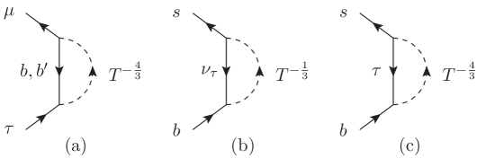
Figure 6: The Feynman diagram for (a) $\tau\rightarrow\mu\gamma$, and (b,c) $b\rightarrow s\gamma(g)$ transition. The external photon (gluon), which is not shown in the illustration, can attach to any charged(color) line in the loop.

The rare $\tau\rightarrow\mu\gamma$ transition can be induced when both $\lambda^{T}_{\tau b^{\prime}}$ and $\lambda^{T}_{\mu b^{\prime}}$ are nonzero. The 1-loop diagram are shown in Fig.6(a).

The dipole $\tau\rightarrow\mu\gamma$ amplitude can be parameterized as

$$i{\cal M}^{\mu}=i\,\left[\bar{\mu}\left(i\sigma^{\mu\nu}k_{\nu}\right)(d^{\tau\mu}_{R}\hat{R}+d^{\tau\mu}_{L}\hat{L})\tau\right]\,,$$ (89)

where $k$ is the photon momentum transfer. If ignoring the muon mass, the partial decay width is given as[114]

$$\Gamma(\tau\rightarrow\mu\gamma)\simeq\frac{m_{\tau}^{3}}{16\pi}(|d^{\tau\mu}_{R}|^{2}+|d^{\tau\mu}_{L}|^{2})\,.$$ (90)

Since the leptoquark $T(D)$ only couples to the LH(RH) charged leptons, it contributes solely to $d^{\tau\mu}_{R(L)}$.

If ignoring the charged lepton masses in the loop, the dipole transition coefficient can be easily calculated to be

$$d^{\tau\mu}_{R}={eN_{c}m_{\tau}\over 16\pi^{2}M_{T}^{2}}\{ \lambda^{T}_{\tau b^{\prime}}(\lambda^{T}_{\mu b^{\prime}})^{*}\beta^{\prime}_{T}[-Q_{T}R_{S}(\beta^{\prime}_{T})+Q_{(b^{\prime})^{c}}R_{F}(\beta^{\prime}_{T})]$$ (91)

$$+ \lambda^{T}_{\tau b}(\lambda^{T}_{\mu b})^{*}\beta_{T}[-Q_{T}R_{S}(\beta_{T})+Q_{(b)^{c}}R_{F}(\beta_{T})]\;\}\,.$$

In the above, $\beta^{\prime}_{T}\equiv(M_{T}/M_{b^{\prime}})^{2}$, $\beta_{T}\equiv(M_{T}/m_{b})^{2}$, $Q_{T}$($Q_{(b^{(^{\prime})})^{c}}$) is the electric charge of the scalar(fermion) in the loop, and the loop functions,

$$R_{S}(x) = {2+3x-6x^{2}+x^{3}+6x\ln x\over 12(1-x)^{4}}\,,\;\mbox{and}$$

$$R_{F}(x) = \frac{R_{S}(1/x)}{x}={1-6x+3x^{2}+2x^{3}-6x^{2}\ln x\over 12(1-x)^{4}}\,,$$ (92)

correspond to the contributions where the external photon attached to the scalar and fermion line in the loop, respectively. Both functions have the same limit $1/24$ when $x\rightarrow 1$. When $x\gg 1$, $R_{S}(x)\rightarrow 1/12x$ and $R_{F}(x)\rightarrow 1/6x$. Note the fermionic and bosonic contributions have opposite signs, and the charged fermion in the loop is the anti-$b^{(^{\prime})}$.

Similarly, the contribution from the diagram with leptoquark $D^{-\frac{2}{3}}$ and $b^{(^{\prime})}$ running in the loop yields

$$d^{\tau\mu}_{L}={eN_{c}m_{\tau}\over 32\pi^{2}M_{D}^{2}} \left\{\lambda^{D}_{\tau b^{\prime}}(\lambda^{D}_{\mu b^{\prime}})^{*}\beta^{\prime}_{D}\left[+\frac{2}{3}R_{S}(\beta^{\prime}_{D})-\frac{1}{3}R_{F}(\beta^{\prime}_{D})\right]\right.$$ (93)

$$+ \left.\lambda^{D}_{\tau b}(\lambda^{D}_{\mu b})^{*}\beta_{D}\left[+\frac{2}{3}R_{S}(\beta_{D})-\frac{1}{3}R_{F}(\beta_{D})\right]\;\right\}\,.$$

As discussed in Sec.III.2, we set $\lambda^{D}_{\mu b^{\prime}}=0$ in ( Sol-2) to avoid the dangerous $\mu\rightarrow e\gamma$ transition. Then, we obtain

$$d^{\tau\mu}_{L}\simeq{eN_{c}m_{\tau}\over 32\pi^{2}M_{D}^{2}}\lambda^{D}_{\tau b}(\lambda^{D}_{\mu b})^{*}\beta_{D}\left[\frac{2}{3}R_{S}(\beta_{D})-\frac{1}{3}R_{F}(\beta_{D})\right]\simeq 0\,,$$ (94)

and due to the accidental cancellation in the squared bracket, it vanishes in the limit of $m_{b}\ll m_{D}$ in this case. Therefore, only $d^{\tau\mu}_{R}$ needs to be taken into account. From $\tau_{\tau}=(290.3\pm 0.5)\times 10^{-15}s$[1], the branching ratio of this rare process is

$${\cal B}(\tau\rightarrow\mu\gamma) = \Gamma(\tau\rightarrow\mu\gamma)/\Gamma_{\tau}$$ (95)

$$\simeq 5.14\times 10^{-6}\left|\lambda^{T}_{\tau b^{\prime}}(\lambda^{T}_{\mu b^{\prime}})^{*}\frac{\beta^{\prime}_{T}}{3}[4R_{S}(\beta^{\prime}_{T})+R_{F}(\beta^{\prime}_{T})]+\frac{\lambda^{T}_{\tau b}(\lambda^{T}_{\mu b})^{*}}{6}\right|^{2}\times\left({\mbox{TeV}\over M_{T}}\right)^{4}\,.$$

The current experimental bound, ${\cal B}(\tau\rightarrow\mu\gamma)<4.4\times 10^{-8}$[131], sets an upper bound

$$\left|\lambda^{T}_{\tau b^{\prime}}(\lambda^{T}_{\mu b^{\prime}})^{*}\frac{4\beta^{\prime}_{T}}{3}[R_{S}(\beta^{\prime}_{T})+R_{F}(\beta^{\prime}_{T})]+\frac{\lambda^{T}_{\tau b}(\lambda^{T}_{\mu b})^{*}}{6}\right|<0.092\times\left({M_{T}\over\mbox{TeV}}\right)^{2}\,.$$ (96)

On the other hand, if both $\lambda^{D}_{\tau b^{\prime}}$ and $\lambda^{D}_{eb^{\prime}}$ present, we have

$$d^{\tau e}_{L}\simeq{eN_{c}m_{\tau}\over 16\pi^{2}M_{D}^{2}}{\lambda^{D}_{\tau b^{\prime}}(\lambda^{D}_{\mu b^{\prime}})^{*}\beta^{\prime}_{D}\over 6}\left[2R_{S}(\beta^{\prime}_{D})-R_{F}(\beta^{\prime}_{D})\right]$$ (97)

for $\tau\rightarrow e\gamma$ transition. From ${\cal B}(\tau\rightarrow e\gamma)<3.3\times 10^{-8}$ [131], it gives a weak bound

$$\left|\lambda^{D}_{\tau b^{\prime}}(\lambda^{D}_{eb^{\prime}})^{*}\right|<16.93\times\left({M_{D}\over\mathrm{TeV}}\right)^{2}$$ (98)

for $\beta^{\prime}_{D}=(1.0/1.5)^{2}$.

IV.6 $b\rightarrow s\gamma$

Similar to the previous discussion on $\tau\rightarrow\mu\gamma$, the $b\rightarrow s\gamma(g)$ transition can be induced when both $\lambda^{T}_{\tau b}$ and $\lambda^{T}_{\tau s}$ are nonzero, see Fig.6(b,c). Moreover, the fermion masses, $m_{\tau}$ or $m_{\nu_{\tau}}$, can be ignored, which corresponds to the $\beta_{T}\gg 1$ limit. From Eq.(92), it is easy to see that $R_{S}(x)\rightarrow 1/(12x)$ and $R_{F}(x)\rightarrow 1/(6x)$ when $x\gg 1$. Therefore, by plugging in the electric charges in the loop, the $b\rightarrow s\gamma$ transition amplitude can readily read as

$$i{\cal M}^{\mu}(b\rightarrow s\gamma)\simeq i{em_{b}\over 16\pi^{2}}{\lambda^{T}_{\tau b}(\lambda^{T}_{\tau s})^{*}\over 12m_{T}^{2}}\left[-\frac{1}{2}\left(-\frac{1}{3}\right)-\left(-\frac{1}{4}\right)+2(1)\right]\left[\bar{s}\left(i\sigma^{\mu\nu}k_{\nu}\right)\hat{R}b\right]\,.$$ (99)

The first one-half factor comes from the $T^{-\frac{1}{3}}$ Yukawa couplings which associate with the $(1/\sqrt{2})$ normalization, see Eq.(11), and the factor 2 in the last term comes from the anti-tau contribution. We also need to consider $b\rightarrow sg$ transition because the RGE running will generate the $b\rightarrow s\gamma$ operator at the low energy. Because the gluon can only couple to the leptoquark, the amplitude reads

$$i{\cal M}^{\mu}(b\rightarrow sg)\simeq i{g_{s}m_{b}\over 16\pi^{2}}{\lambda^{T}_{\tau b}(\lambda^{T}_{\tau s})^{*}\over 12m_{T}^{2}}\left[-\frac{1}{2}-\left(1\right)\right]\left[\bar{s}\left(iT^{(a)}\sigma^{\mu\nu}k_{\nu}\right)\hat{R}b\right]\,.$$ (100)

where $T^{(a)}$ is the $SU(3)_{c}$ generator.

Conventionally, the relevant effective Hamiltonian is given as

$${\cal H}^{b\rightarrow s\gamma}_{eff}=-\frac{4G_{F}}{\sqrt{2}}V_{tb}V_{ts}^{*}({\cal C}_{7}{\cal O}_{7}+{\cal C}_{8}{\cal O}_{8})\,,$$ (101)

with

$${\cal O}_{7} = \frac{e}{16\pi^{2}}m_{b}\bar{s}\sigma^{\mu\nu}\hat{R}bF_{\mu\nu}\,,$$

$${\cal O}_{8} = \frac{g_{s}}{16\pi^{2}}m_{b}\bar{s}_{\alpha}\sigma^{\mu\nu}\hat{R}T^{(a)}_{\alpha\beta}b_{\beta}G^{(a)}_{\mu\nu}\,,$$ (102)

In our model, the Wilson coefficients for ${\cal O}_{7}$ and ${\cal O}_{8}$ can be identified as

$${\cal C}_{7}\simeq{1\over 2\sqrt{2}G_{F}V_{tb}V_{ts}^{*}}{7\lambda^{T}_{\tau b}(\lambda^{T}_{\tau s})^{*}\over 48M_{T}^{2}}\,,$$

$${\cal C}_{8}\simeq-{1\over 2\sqrt{2}G_{F}V_{tb}V_{ts}^{*}}{\lambda^{T}_{\tau b}(\lambda^{T}_{\tau s})^{*}\over 8M_{T}^{2}}\,.$$ (103)

The current experimental measurement, $Br^{Exp}(b\rightarrow s\gamma)=(3.32\pm 0.15)\times 10^{-4}$[132], and the SM prediction, $Br^{SM}(b\rightarrow s\gamma)=(3.36\pm 0.23)\times 10^{-4}$[133, 134], agree with each other and set constraints on the NP contribution. Following Refs.[78, 81, 128], we adopt the $2\sigma$ bound for the NP that $|{\cal C}_{7}+0.19{\cal C}_{8}|\lesssim 0.06$, which leads to $|\lambda^{T}_{\tau b}(\lambda^{T}_{\tau s})^{*}|<0.55$. This limit is much weaker than the one obtained from $\triangle M_{s}$.

IV.7 Neutrino oscillation data

As discussed before, the vanishing $\lambda^{T}_{ed_{i}}$ are preferred by phenomenological consideration. It is then followed by a robust prediction that ${\cal M}_{ee}=0$, and the neutrinoless double beta decay mediated by ${\cal M}_{ee}$ vanishes as well. Therefore, the neutrino mass is predicted to be the normal hierarchical(NH). Later we should discuss the consequence if this vanishing-$\lambda^{T}_{ed_{i}}$ assumption is relaxed.

A comprehensive numerical fit to the neutrino data is unnecessary to understand the physics, and it is beyond the scope of this paper as well. For simplicity, we assume all the Yukawa couplings are real, and thus all the CP phases in the neutrino mixings vanish. However, this model has no problem to fit the CP violation phases of any values once the requirement of all the Yukawa couplings being real is lifted. Moreover, to adhere to the philosophy of using the least number of real parameters, only two more Yukawa couplings, $\lambda^{D}_{\tau b^{\prime}}$ and $\lambda^{D}_{\tau b}$, are introduced to fit the neutrino data. Together with $\mbox{MinS}_{T}$, we make use of eleven Yukawa couplings, and the complete minimal set of parameter is

$$\mbox{MinS}=\mbox{MinS}_{T}\cup\left\{\lambda^{D}_{eb^{\prime}},\lambda^{D}_{\tau b^{\prime}},\lambda^{D}_{\mu b},\lambda^{D}_{\tau b},\lambda^{S}_{eb^{\prime}},\lambda^{S}_{\mu b}\right\}\,.$$ (104)

Assuming that $M_{D}\simeq M_{T}\simeq M_{LQ}$, the neutrino mass matrix takes the form

$${\cal M}^{\nu}\simeq N^{\nu}\left(\begin{array}[]{ccc}0&\lambda^{D}_{eb^{\prime}}\lambda^{T}_{\mu b^{\prime}}&\lambda^{D}_{eb^{\prime}}\lambda^{T}_{\tau b^{\prime}}\\ \lambda^{D}_{eb^{\prime}}\lambda^{T}_{\mu b^{\prime}}&2\rho_{b}\lambda^{D}_{\mu b}\lambda^{T}_{\mu b}&\rho_{b}(\lambda^{D}_{\mu b}\lambda^{T}_{\tau b}+\lambda^{D}_{\tau b}\lambda^{T}_{\mu b})+\lambda^{D}_{\mu b^{\prime}}\lambda^{T}_{\tau b^{\prime}}\\ \lambda^{D}_{eb^{\prime}}\lambda^{T}_{\tau b^{\prime}}&\rho_{b}(\lambda^{D}_{\mu b}\lambda^{T}_{\tau b}+\lambda^{D}_{\tau b}\lambda^{T}_{\mu b})+\lambda^{D}_{\mu b^{\prime}}\lambda^{T}_{\tau b^{\prime}}&2\rho_{b}\lambda^{D}_{\tau b}\lambda^{T}_{\tau b}+2\lambda^{D}_{\tau b^{\prime}}\lambda^{T}_{\tau b^{\prime}}\\ \end{array}\right)\,,$$ (105)

where $\rho_{b}=m_{b}/M_{b^{\prime}}$ and $N^{\nu}={3\mu_{3}v_{0}M_{b^{\prime}}\over 32\pi^{2}M^{2}_{LQ}}$. Note that the leptoquark Yukawa couplings are tightly entangled with the neutrino mass matrix. For instance, $\lambda^{T}_{\tau b^{\prime}}/\lambda^{T}_{\mu b^{\prime}}={\cal M}^{\nu}_{e\tau}/{\cal M}^{\nu}_{e\mu}$ is required by this minimal assumption.

For illustration, we consider an approximate neutrino mass matrix

$${\cal M}^{\nu}\simeq\left(\begin{array}[]{ccc}0&0.90792&0.13812\\ 0.90792&-2.4923&-2.7643\\ 0.13812&-2.7643&-1.9353\\ \end{array}\right)\times 10^{-2}\mathrm{eV}\,,$$ (106)

with all elements being real. It leads to the following mixing angles and mass squared differences

$$\theta_{12}\simeq 33.0^{\circ}\,,\;\theta_{23}\simeq 48.7^{\circ}\,,\;\theta_{13}\simeq 8.6^{\circ}\,,\;\delta_{CP}=0^{\circ}\,,$$

$$\triangle m_{21}^{2}\sim 7.47\times 10^{-5}\mbox{eV}^{2}\,,\;\triangle m_{31}^{2}\sim 2.53\times 10^{-3}\mbox{eV}^{2}\,.$$ (107)

Note all of the above values, except $\delta_{CP}$, are inside the $1\sigma$ best fit (with SK atmospheric data) range for the normal ordering given by [135],

$$\theta_{12}\in(32.7-34.21)^{\circ}\,,\;\theta_{23}\in(48.0-50.1)^{\circ}\,,\;\theta_{13}\in(8.45-8.69)^{\circ}\,,\;\delta_{CP}\in(173-224)^{\circ}\,,$$

$$\triangle m_{21}^{2}\in(7.22-7.63)\times 10^{-5}\mbox{eV}^{2}\,,\;\triangle m_{31}^{2}\in(2.489-2.543)\times 10^{-3}\mbox{eV}^{2}\,.$$ (108)

This example neutrino mass matrix captures the essential features of the current neutrino data. A better fitting to the neutrino oscillation data, including the phase, by using more(complex) model parameters is expected.

In order to reproduce the neutrino mass matrix, the second solution to $\triangle a_{e,\mu}$, Eq.(44), must be adopted. Because the first solution $\triangle a_{e,\mu}$, Eq.(43), requires $\mu_{1}\gg M_{LQ}$ to render mass matrix elements of about the same order, as shown in Eq.(106). All the best fit central values for $b\rightarrow s\mu\mu$, $\triangle a_{e,\mu}$, CAA, and the approximate neutrino mass matrix shown in Eq.(106) can be easily accommodated with the specified non-vanishing parameters in the model. Since $(M_{b^{\prime}}/m_{b})\gg 1$, $\lambda^{D}_{\mu b},\lambda^{S}_{eb^{\prime}}>\sqrt{4\pi}$ are required if aiming for explaining the central values of $\triangle a_{e,\mu}$. However, reliable nonperturbative treatment is beyond the scope of this paper. Instead, we consider the $1\sigma$ ranges of best fit for $b\rightarrow s\mu\bar{\mu}$ and $\triangle a_{e}$. As an example, below is one of the viable sets of model parameters for $\triangle a_{e}=-5.1[1.8]\times 10^{-13}$ and $C_{9}=-C_{10}=-0.351$,

$$M_{LQ}=1.0\,\mathrm{TeV}\,,\,M_{b^{\prime}}=1.5\,\mathrm{TeV}\,,\,\mu_{1}=2.298[-0.818]\,\mathrm{TeV}\,,\,\mu_{3}=0.513\,\mathrm{keV}\,,s_{1}=0.039$$

$$\lambda^{T}_{\mu b^{\prime}}=-3.34514\,,\,\lambda^{T}_{\tau b^{\prime}}=-0.508902\,,\,\lambda^{T}_{\mu b}=-0.728492\,,$$

$$\lambda^{T}_{\tau b}=0.929742\,,\,\,\lambda^{T}_{\tau s}=-0.076018\,,$$

$$\lambda^{D}_{eb^{\prime}}=-0.00151\,,\,\lambda^{D}_{\mu b}=3.4\,,\,\lambda^{D}_{\tau b^{\prime}}=0.00760\,,\,\lambda^{D}_{\tau b}=-0.58293\,,$$

$$\lambda^{S}_{eb^{\prime}}=3.4\,,\,\lambda^{S}_{\mu b}=-0.088264[0.24798]\,,\,$$ (109)

and all the other Yukawa couplings are set to zero. This specific set of model parameters also predicts $\triangle M_{s}\simeq 1.06\,\triangle M_{s}^{SM}$, $R^{\nu}_{K^{(*)}}=1.21$,

$${\cal B}(\tau\rightarrow\mu\gamma)=6.0\times 10^{-9}\,,\;{\cal B}(\tau\rightarrow e\gamma)=1.5\times 10^{-20}\,,\;{\cal B}(B^{+}\rightarrow K^{+}\mu^{+}\tau^{-})=1.4\times 10^{-5}\,,$$ (110)

and pass all experimental limits we have considered, the last column in Tables 5 and 6.

Note that $\lambda^{T}_{\mu b^{\prime}}$, $\lambda^{D}_{\mu b}$, and $\lambda^{S}_{eb^{\prime}}$ in Eq.(109) are close to but below the nonperturbative limit $\sqrt{4\pi}$. However, this is because we want to use the minimal number of model parameters. For instance, if the complex Yukawa is allowed, the degrees of freedom are doubled. Lowering $M_{b^{\prime}}$ and increasing $\mu_{1}$ can both make $\lambda^{D}_{\mu b}$ and $\lambda^{S}_{eb^{\prime}}$ smaller as well. We have no doubt that a better fitting can be achieved in this model by using more (complex) free parameters. But we are content with the demonstration about the ability of this model to accommodate all the observed anomalies and explain the pattern of the observed neutrino data with minimal number of real parameters.

IV.8 $0\nu\beta\beta$ decay

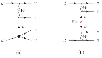
Figure 7: The Feynman diagrams for $0\nu\beta\beta$ decay (a) mediated by the $T\mathchar 45\relax D$ mixing, and (b) mediated by the neutrino Majorana mass.

The mixing between $T$ and $D$ breaks the global lepton number, see Appendix B. Here, we consider whether the neutrinoless double beta decay can be generated beyond the contribution from the neutrino Majorana mass. From the low energy effective Hamiltonian, together with the SM CC interaction, the lepton number violating charged current operators can induce the $0\nu\beta\beta$ process via the diagram, see Fig.7(a). By order of magnitude estimation, the absolute value of the amplitude strength relative to the usual one mediated by the neutrino Majorana mass, Fig.7(b), is given by

$$\left|{{\cal M}_{TD}\over{\cal M}_{m_{\nu}}}\right|\simeq{\lambda_{T}\lambda_{D}\mu_{3}v_{0}\over M_{T}^{2}M_{D}^{2}}\frac{M_{W}^{2}\langle p\rangle}{g_{2}^{2}{\cal M}^{\nu}_{ee}}\simeq 10^{-5}\left(\frac{1\,\mbox{TeV}}{M_{LQ}}\right)^{4}\ll 1\,.$$ (111)

In arriving the above value, we take $\mu_{3}=0.5\mathrm{keV}$, $\langle p\rangle\sim 1\,\mathrm{MeV}$ for the typical average momentum transfer in the $0\nu\beta\beta$ process and assume ${\cal M}^{\nu}_{ee}\sim 0.01\mathrm{eV}$ for comparison. Thus, this tree-level process mediated by $T$ and $D$ can be ignored.

IV.9 A recap

After taking into account all the phenomenological limits, we found the following simple assignment with minimal number of real parameters,

$$M_{LQ}\simeq 1.0\,\mathrm{TeV}\,,\,M_{b^{\prime}}=1.5\,\mathrm{TeV}\,,\,\mu_{1}=2.3[-0.82]\,\mathrm{TeV}\,,\,\mu_{3}\simeq 0.5\,\mathrm{keV}\,,$$

$$\mu_{1}\lambda^{S}_{eb^{\prime}}\lambda^{D}_{eb^{\prime}}=-12[4]\mathrm{GeV}\,,\;\mu_{1}\lambda^{S}_{\mu b}\lambda^{D}_{\mu b}=-690\mathrm{GeV}\,,$$

$$\theta_{2}=\theta_{3}=0\,,\;\sin\theta_{1}=0.039\,,$$

$$\lambda^{T}_{\mu b^{\prime}}\simeq-3.3\,,\,\lambda^{T}_{\tau b^{\prime}}\simeq-0.51\,,\,\lambda^{T}_{\mu b}\simeq-0.72\,,\,\lambda^{T}_{\tau b}\simeq 0.93\,,\,\lambda^{T}_{\tau s}\simeq-0.08\,,$$

$$\lambda^{D}_{eb^{\prime}}\simeq-0.002\,,\,\lambda^{D}_{\mu b}\simeq 3.4\,,\,\lambda^{D}_{\tau b^{\prime}}\simeq 0.008\,,\,\lambda^{D}_{\tau b}\simeq-0.58\,,$$ (112)

is able to accommodate $\triangle a_{e}^{Cs}[\triangle a_{e}^{Rb}]$, $\triangle a_{\mu}$, the Cabibbo angle, and $b\rightarrow s\mu\mu$ anomalies simultaneously. Moreover, the resulting neutrino mass pattern is very close to the observed one.

V Discussion

V.1 Neutrino mass hierarchy and neutrinoless double beta decay

Because we set $\lambda^{T}_{ed_{i}}=0(i=d,s,b,b^{\prime})$, the neutrino mass element $M^{\nu}_{ee}$ vanishes and the neutrino mass is of the NH type. Since we have used $\lambda^{S}_{eb^{\prime}}$ to explain the observed $\triangle a_{e}$, adding $\lambda^{T}_{eb^{\prime}}$ is the minimal extension to yield a non-zero $M^{\nu}_{ee}$. Together with $\lambda^{T}_{\mu b}$ and $\lambda^{T}_{\mu b^{\prime}}$, the augmentation of $\lambda^{T}_{eb^{\prime}}$ leads to an effective Hamiltonian,

$$H\supset\frac{{\cal C}_{\mu e}}{4M_{T}^{2}}(\bar{u}\gamma^{\mu}\hat{L}u)(\bar{\mu}\gamma_{\mu}\hat{L}e)+H.c.\,,$$ (113)

where

$${\cal C}_{\mu e}=\lambda^{T}_{eb^{\prime}}(\widetilde{V}_{ub^{\prime}})^{*}\left[\widetilde{V}_{ub}(\lambda^{T}_{\mu b})^{*}+\widetilde{V}_{ub^{\prime}}(\lambda^{T}_{\mu b^{\prime}})^{*}\right]\,.$$ (114)

Numerically,

$${\cal C}_{\mu e}\simeq 1.44\times 10^{-3}\lambda^{T}_{eb^{\prime}}(\lambda^{T}_{\mu b^{\prime}})^{*}+1.37\times 10^{-4}\lambda^{T}_{eb^{\prime}}(\lambda^{T}_{\mu b})^{*}\,,$$ (115)

if we set $s_{1}=0.039$ and $\widetilde{V}_{ub}=0.00361$.

The Wilson coefficient is severely constrained, ${\cal C}_{\mu e}<9.61\times 10^{-5}$, from the experimental limit of $\mu\mathchar 45\relax e$ conversion rate[136, 116]. Namely, $\lambda^{T}_{eb^{\prime}}(\lambda^{T}_{\mu b^{\prime}})^{*}\lesssim 0.07$ unless the cancellation is arranged in Eq.(115). Moreover, in this model, the ratio of neutrino mass element $M^{\nu}_{ee}$ to $M^{\nu}_{e\mu}$, see Eq.(105),

$$\frac{M^{\nu}_{ee}}{M^{\nu}_{e\mu}}={2M_{b^{\prime}}\lambda^{D}_{eb^{\prime}}\lambda^{T}_{eb^{\prime}}\over M_{b^{\prime}}\lambda^{D}_{eb^{\prime}}\lambda^{T}_{\mu b^{\prime}}}=\frac{2\lambda^{T}_{eb^{\prime}}}{\lambda^{T}_{\mu b^{\prime}}}\,,$$ (116)

should be around $\sim{\cal O}(1)$ and $\sim{\cal O}(10)$ for the NH and Inverted Hierarchy (IH) type, respectively. Since we need $\lambda^{T}_{\mu b^{\prime}}\sim{\cal O}(1)$ to accommodate the b-anomalies, that implies $\frac{M^{\nu}_{ee}}{M^{\nu}_{e\mu}}\lesssim 0.07$. Thus, even if we include a non-zero $\lambda^{T}_{eb^{\prime}}$ to generate the $ee$-component of $M_{\nu}$, the neutrino mass is still of the NH type, and roughly $|M^{\nu}_{ee}|\lesssim 3\times 10^{-4}\mathrm{eV}$. The precision required is beyond the capabilities of the near future experiments[137].

V.2 Some phenomenological consequences at the colliders

The smoking gun signature of this model will be the discovery of $b^{\prime}$ and the three scalar leptoquarks. Once their quantum numbers are identified, the gauge invariant allowed Yukawa couplings and the mechanisms to address the anomalies discussed in the paper follow automatically. The collider physics of leptoquarks have been extensively studied before, and thus we do not have much to add. The readers interested in this topic are referred to the comprehensive review [138] and the references therein. In the paper, we should concentrate on the flavor physics at around or below the Z pole.

However, it is worthy to point out the nontrivial decay branching ratios of the exotic color states. If we assume the mixings among the leptoquarks are small, their isospin members should be approximately degenerate in mass. Then, the decays are dominated by 2-body decay with two SM fermions in the final states. From the Yukawa couplings shown in Eq.(109), the decay branching ratio of leptoquarks can be easily read. For $T^{-\frac{1}{3}}$, its decay branching ratios are

$${\cal B}(T^{-\frac{1}{3}}\rightarrow b\nu_{\mu})\simeq 18.9\%\,,\;{\cal B}(T^{-\frac{1}{3}}\rightarrow b\nu_{\tau})\simeq 30.9\%\,,\;{\cal B}(T^{-\frac{1}{3}}\rightarrow s\nu_{\tau})\simeq 2.1\times 10^{-3}\,,$$

$${\cal B}(T^{-\frac{1}{3}}\rightarrow\tau t)\simeq 30.8\%\,,\;{\cal B}(T^{-\frac{1}{3}}\rightarrow\mu t)\simeq 18.9\%\,,\;{\cal B}(T^{-\frac{1}{3}}\rightarrow\tau c)\simeq 2.0\times 10^{-3}\,.$$ (117)

For $T^{\frac{2}{3}}$ and $T^{\frac{4}{3}}$, the corresponding decay branching ratios are

$${\cal B}(T^{\frac{2}{3}}\rightarrow t\nu_{\mu})\simeq 37.9\%\,,\;{\cal B}(T^{\frac{2}{3}}\rightarrow t\nu_{\tau})\simeq 61.7\%\,,\;{\cal B}(T^{\frac{2}{3}}\rightarrow c\nu_{\tau})\simeq 0.4\%\,,$$

$${\cal B}(T^{-\frac{4}{3}}\rightarrow b\mu^{-})\simeq 37.9\%\,,\;{\cal B}(T^{-\frac{4}{3}}\rightarrow b\tau^{-})\simeq 61.7\%\,,\;{\cal B}(T^{-\frac{4}{3}}\rightarrow s\tau^{-})\simeq 0.4\%\,.$$ (118)

Finally, we have

$${\cal B}(D^{-\frac{1}{3}}\rightarrow b\bar{\nu}_{\mu})\simeq 97.1\%\,,\;{\cal B}(D^{-\frac{1}{3}}\rightarrow b\bar{\nu}_{\tau})\simeq 2.9\%\,,$$

$${\cal B}(D^{\frac{2}{3}}\rightarrow b\mu^{+})\simeq 97.1\%\,,\;{\cal B}(D^{\frac{2}{3}}\rightarrow b\tau^{+})\simeq 2.9\%\,,$$

$${\cal B}(S^{\frac{2}{3}}\rightarrow b\mu^{+})\simeq 100\%\,,$$ (119)

for $D$ and $S$ leptoquarks.

The dominate decay modes of $b^{\prime}$ are $b^{\prime}\rightarrow LQ+l$, and $b^{\prime}\rightarrow W^{-}u_{i}(u_{i}=u,c,t)$ through the mixing of $\widetilde{V}_{u_{i}b^{\prime}}$. Comparing to $M_{b^{\prime}}$, the masses of final state particles can be ignored. The width for $b^{\prime}\rightarrow Wu_{i}$ is simply given by

$$\Gamma(b^{\prime}\rightarrow u_{i}W^{-})\simeq\frac{G_{F}|\widetilde{V}_{u_{i}b^{\prime}}|^{2}M_{b^{\prime}}^{3}}{8\sqrt{2}\pi}\,,$$ (120)

and

$$\Gamma(b^{\prime}\rightarrow\bar{\nu_{i}}T^{-\frac{1}{3}})\simeq\frac{|\lambda^{T}_{l_{i}b^{\prime}}|^{2}}{64\pi}M_{b^{\prime}}\left(1-\frac{M_{T}^{2}}{M_{b^{\prime}}^{2}}\right)^{2}\,,\;\Gamma(b^{\prime}\rightarrow\ell^{+}_{i}T^{-\frac{4}{3}})\simeq\frac{|\lambda^{T}_{l_{i}b^{\prime}}|^{2}}{32\pi}M_{b^{\prime}}\left(1-\frac{M_{T}^{2}}{M_{b^{\prime}}^{2}}\right)^{2}\,,$$

$$\Gamma(b^{\prime}\rightarrow\nu_{i}D^{-\frac{1}{3}})\simeq\Gamma(b^{\prime}\rightarrow\ell^{-}_{i}D^{\frac{2}{3}})\simeq\frac{|\lambda^{D}_{l_{i}b^{\prime}}|^{2}}{64\pi}M_{b^{\prime}}\left(1-\frac{M_{D}^{2}}{M_{b^{\prime}}^{2}}\right)^{2}\,,$$

$$\Gamma(b^{\prime}\rightarrow\ell_{i}S^{\frac{2}{3}})\simeq\frac{|\lambda^{S}_{l_{i}b^{\prime}}|^{2}}{32\pi}M_{b^{\prime}}\left(1-\frac{M_{S}^{2}}{M_{b^{\prime}}^{2}}\right)^{2}\,.\;$$ (121)

The Yukawa coupling between $b^{\prime}$ and the SM Higgs is through the $b^{\prime}\mathchar 45\relax d$ mixing. So the resulting Yukawa coupling gets double suppression from the small $\theta_{1}$ and the ratio of $m_{d}/v_{0}$, and so the $b^{\prime}\rightarrow Hd$ decay can be ignored. Similarly the decays of $b^{\prime}\rightarrow Z^{0}d_{i}$ can be ignored as well. By plugging in the parameters we found, the total decay width of $b^{\prime}$ is $\Gamma_{b^{\prime}}\simeq 134.0\mathrm{GeV}$, and the branching ratios are

$${\cal B}(b^{\prime}\rightarrow uW^{-})\simeq 1.2\%\,,\;{\cal B}(b^{\prime}\rightarrow cW^{-})\simeq 6\times 10^{-4}\,,\;{\cal B}(b^{\prime}\rightarrow tW^{-})\simeq 9\times 10^{-7}\,,$$

$${\cal B}(b^{\prime}\rightarrow\bar{\nu}T^{-\frac{1}{3}})\simeq 19.7\%\,,\;{\cal B}(b^{\prime}\rightarrow\mu^{+}T^{-\frac{4}{3}})\simeq 38.5\%\,,$$

$${\cal B}(b^{\prime}\rightarrow\tau^{+}T^{-\frac{4}{3}})\simeq 0.9\%\,,\;{\cal B}(b^{\prime}\rightarrow eS^{\frac{2}{3}})\simeq 39.7\%\,,$$ (122)

for $M_{LQ}=1\mathrm{TeV}$ and $M_{b^{\prime}}=1.5\mathrm{TeV}$.

We stress that the above decay branching ratios are the result of using the example parameter set given in Eq.(109). The decay branching ratios depend strongly on the model parameters, and the branching ratio pattern varies dramatically from one neutrino mass matrix to another. However, one can see that the decay pattern of the heavy exotic color states in this example solution is very different from the working assumption of 100% $b^{\prime}\rightarrow tW,Zb,Hb$ used for singlet $b^{\prime}$ and other assumption used for the leptoquark searches at the colliders.

Before closing this section, we want to point out some potentially interesting FCNC top 3-body decays in this framework. From the example solution, we have

$${\cal B}(t\rightarrow u\tau^{+}\mu^{-})\simeq{\cal B}(t\rightarrow u\mu^{+}\mu^{-})\simeq 2\times 10^{-9}\,.$$ (123)

With an integrated luminosity of $3\mbox{ab}^{-1}$ and CM energy at $13\mathrm{TeV}$, about $2.5\times 10^{9}$ top quark pair events will be produced at the LHC. Therefore, only $\sim 5$ events which include at least one top decaying in these 3-body FCNC are expected. However, the 3-body FCNC $t\rightarrow cl_{i}l_{j}$ branching ratios change if adopting a different solution. During our numerical study, we observe that in some cases there are one or two of them at the ${\cal O}(10^{-7})$ level, which might be detectable at the LHC. See [139] for the prospect of studying these potentially interesting 3-body top decay modes at the LHC.

V.3 Flavor violating neutral current processes

A few comments on the data fitting are in order: From Table 5, one sees that the fit almost saturates, $\sim 80\%$, of the current limit on decay branching ratio $B^{+}\rightarrow K^{+}\mu^{+}\tau^{-}$. Moreover, the fit is very close to the $2\sigma$ limit from $B_{s}-\overline{B}_{s}$ mixing. The solution seems to be stretched to the limit, and the discovery of lepton flavor violating signals are around the corners. However, this is the trade-off of using minimal number of parameters to reproduce all the central values. If instead aiming for the $1\sigma$ values, both can be reduced by half. In addition, the Yukawa couplings are tightly connected with the neutrino mass matrix. During our numerical study, we observe that $D^{+}\rightarrow\pi^{+}\mu^{+}\mu^{-}$ and $B^{+}\rightarrow K^{+}\mu^{+}\tau^{-}$ can be far below their experimental upper bounds while $\tau\rightarrow\mu\gamma$ close to the current experimental limit if using some different neutrino mass matrix or relaxing the strict relationship that $\widetilde{V}^{*}_{cb}\lambda^{T}_{\mu b}+\widetilde{V}^{*}_{cb^{\prime}}\lambda^{T}_{\mu b^{\prime}}=0$. Therefore, the model has vast parameter space to accommodate the anomalies with diversified predictions, and we cannot conclusively predict the pattern of the rare process rates at the moment.

However, because we need $\lambda^{T}_{\tau b}\lambda^{T}_{\tau s}\neq 0$ to explain the $b\rightarrow s\mu\mu$ anomaly, the $b\rightarrow s\tau\tau$ transition will be always generated at the tree-level. From the example solution, we have

$${\cal H}^{b\rightarrow s\tau\tau}_{eff} \simeq -\frac{G_{F}}{\sqrt{2}}\widetilde{V}_{tb}\widetilde{V}_{ts}^{*}\frac{\alpha}{\pi}{\cal C}^{bs\tau\tau}\left[\bar{s}\gamma^{\alpha}\hat{L}b\right]\left[\bar{\tau}\gamma_{\alpha}(1-\gamma^{5})\tau\right]+H.c.\,,$$

$${\cal C}^{bs\tau\tau} \simeq \frac{\sqrt{2}\pi}{4\alpha}{\lambda^{T}_{\tau b}(\lambda^{T}_{\tau s})^{*}\over\widetilde{V}_{tb}\widetilde{V}_{ts}^{*}G_{F}M_{T}^{2}}=23.2\times\left({\mathrm{TeV}\over M_{T}}\right)^{2}\,,$$ (124)

if taking $\widetilde{V}_{tb}\widetilde{V}_{ts}^{*}=-0.03975$. The additional 1-loop contribution via the box diagram similar to that of $b\rightarrow s\mu\mu$ can be ignored. This Wilson coefficient is roughly six times larger than the SM prediction that ${\cal C}^{bs\tau\tau}_{SM}\sim-4.3$[140, 141, 142], and push the decay branching ratio to $Br(B_{s}\rightarrow\tau^{+}\tau^{-})\simeq 1.6\times 10^{-5}$. Although the above value is still two orders below the relevant experimental upper limit, $\sim{\cal O}(10^{-3})$, for $B_{s}\rightarrow\tau^{+}\tau^{-}$ at LHCb[143] and $B^{+}\rightarrow K^{+}\tau^{+}\tau^{-}$ at BaBar[144], this interesting $b\rightarrow s\tau\tau$ transition could be potentially studied at the LHCb and Belle II[145], or at the Z-pole[146].

V.4 $B\rightarrow D^{(*)}\tau\bar{\nu}$

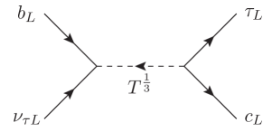
Figure 8: The Feynman diagram for $b\rightarrow c\tau\nu$ transition.

Alongside the $b\rightarrow sl^{+}l^{-}$ anomaly, the global analysis[132, 147, 148, 149, 150] of the $R(D^{(*)})={\cal B}(B\rightarrow D^{(*)}\tau\nu)/{\cal B}(B\rightarrow D^{(*)}\mu\nu)$ data [151, 152, 153, 154, 155, 156] also point to the $\tau\mathchar 45\relax\mu$ lepton flavor universality violation with a significance of $\geq 3\sigma$. In this mode, the $\mbox{MinS}_{T}$ of $\lambda^{T}$ contains the needed tree-level $b\rightarrow c\tau\nu$ operator, Fig.8, to address the $R(D^{(*)})$ problem, and

$${\cal H}^{CC}_{eff}\supset-\left[{\lambda^{T}_{\tau s}(\lambda^{T}_{\tau b})^{*}\widetilde{V}_{cs}+\lambda^{T}_{\tau b}(\lambda^{T}_{\tau b^{\prime}})^{*}\widetilde{V}_{cb^{\prime}}+|\lambda^{T}_{\tau b}|^{2}\widetilde{V}_{cb}\over 4M_{T}^{2}}\right]\left(\bar{c}\gamma^{\alpha}\hat{L}b\right)\left(\bar{\tau}\gamma_{\alpha}\hat{L}\nu_{\tau}\right)+H.c.$$ (125)

This is to compare with the standard effective Hamiltonian

$${\cal H}_{eff}^{b\rightarrow cl\nu}=\frac{4G_{F}}{\sqrt{2}}V_{cb}[(1+{\cal C}_{V_{L}}){\cal O}_{V_{L}}+{\cal C}_{V_{R}}{\cal O}_{V_{R}}+{\cal C}_{S_{L}}{\cal O}_{S_{L}}+{\cal C}_{S_{R}}{\cal O}_{S_{R}}+{\cal C}_{T}{\cal O}_{T}]+H.c.$$ (126)

where

$${\cal O}_{V_{L,R}} = (\bar{c}\gamma^{\mu}b_{L,R})(\bar{l}_{L}\gamma_{\mu}\nu_{lL})\,,$$

$${\cal O}_{S_{L,R}} = (\bar{c}b_{L,R})(\bar{l}_{R}\nu_{lL})\,,\;{\cal O}_{T}=(\bar{c}\sigma^{\mu\nu}b_{L})(\bar{l}_{R}\sigma_{\mu\nu}\nu_{lL})\,.$$ (127)

In this model, the only CC operator can be generated at tree-level is ${\cal O}_{V_{L}}$, thus ${\cal C}_{V_{R}}=0$, ${\cal C}_{S_{R,L}}=0$, and ${\cal C}_{T}=0$. From the global fit with single operator[147], the $R(D^{(*)})$ anomaly can be well addressed if ${\cal C}_{V_{L}}\simeq 0.08$. However, the requirement to retain the $\mu\mathchar 45\relax e$ universality in $b\rightarrow cl\nu$ strictly limits the parameter space. By using the real MinS of parameters, we found the model can render at most ${\cal C}^{NP}_{V_{L}}\lesssim 0.01$. On the other hand, we cannot rule out the possibility that the model has the viable complex number parameter space to accommodate this anomaly with others simultaneously.

On the other hand, this model predicts the lepton universality violation in the $b\rightarrow ul_{i}\nu_{j}(i,j=\mu,\tau)$ transition, see the relevant Wilson coefficients in Table 6. Again, there is no electron counter parts if we use the $\mbox{MinS}_{T}$. From our example solution, the rate of $b\rightarrow u\mu\nu$ could deviate from the SM one by $\sim 40\%$ due to the smallness of $\widetilde{V}_{ub}$ and the interference between the NP and the SM weak interaction. More insights of the intriguing flavor problem are expected if the better experimental measurements on the $b\rightarrow ul\nu$ transitions are available[157].

V.5 Origin of the flavor structure

Not only the subset of parameters are required to explain the anomalies, the nearly vanishing entities in the Yukawa matrices play vital roles to bypass the strong flavor-changing experimental constraints. The next question is how to understand the origin of this staggering flavor pattern. Usually, the flavor pattern is considered within the framework of flavor symmetries. It is highly nontrivial to embed the flavor pattern we found into a flavor symmetry, and it is beyond the scope of this paper. Alternatively, we discuss the possible geometric origin of the flavor pattern in the extra-dimensional theories[158, 159, 160, 161].

A comprehensive fitting, including all the SM fermion masses and mixings, like [162, 163, 164, 165] is also beyond the scope of this paper. Instead, here we only consider how to generate the required flavor pattern of the leptoquark Yukawa coupling shown in Eq.(112). To illustrate, we consider a simple split fermion toy model[161]. We assume all the chiral fermion wave functions are Gaussian locating in a small region, but at different positions, in the fifth dimension. Moreover, all the 5-dim Gaussian distributions are assumed to share a universal width, $\sigma_{SF}$. As for the three leptoquarks, we assume they do not have the zero mode such that their first Kaluza-Klein(KK) mode are naturally heavy. More importantly, this setup forbids the leptoquark to develop VEV and break the $SU(3)_{c}$ symmetry. In addition, the wavefunctions of the first leptoquark KK mode are assumed to be slowly varying in the vicinity of the fermion cluster, and can be approximated as constants. On the other hand, the SM Higgs must acquires the zero mode so that it can develop $v_{0}$ and breaks the SM electroweak symmetry. Then, the 4-dim effective theory is obtained after integrating out the fifth dimension. The effective $\lambda^{s}_{ij}(s=T,D,S)$ Yukawa couplings is determined by the overlapping of two chiral fermions’ 5-dim wave functions times the product of the scalar-specific 5-dim Yukawa coupling and the scalar’s 5-dim wavefunction, denoted as $N_{s}$, in the vicinity where the fermions locate. The 4-dim Yukawa coupling is given by

$$\lambda^{s}_{ij}=N_{s}\,\mbox{Exp}\left[-\frac{(z_{i}-z_{j})^{2}}{2\sigma_{SF}^{2}}\right]\,,\;(s=T,D,S)\,,$$ (128)

where $z_{i}$ is the center location in the fifth dimension of the Gaussian wave function of particle$-i$. It is clear that only the relative distances matter, so we arbitrarily set $z_{\tau_{L}}=0$ for the LH tau. Note that different fermion chiralities are involved for different scalar leptoquark Yukawa couplings. For example, $\lambda^{T}_{ij}$ is determined by the separation between the corresponding LH down-quark($z_{d_{jL}}$) and the LH lepton($z_{\ell_{iL}}$), but $z_{l_{iR}}$ and $z_{d_{jL}}$ are involved for $\lambda^{S}_{ij}$.

For simplicity, we assume the mass and interaction eigenstates coincide for the down-type quarks and the SM charged leptons. We found the flavor structure can be excellently reproduced if the chiral fermion locations in the fifth dimension are

$$\{z_{\tau_{L}},z_{\mu_{L}},z_{e_{L}},z_{\mu_{R}},z_{e_{R}}\} = \{0,\;-0.49,\;7.75[7.80],\;-4.99[-4.72],\;-0.89[-0.97]\}\,,$$

$$\{z_{d_{L}},z_{s_{L}},z_{b_{L}},z_{b^{\prime}_{L}},z_{b_{R}},z_{b^{\prime}_{R}}\} = \{-5.27[-5.53],\;2.86[2.90],\;-2.14[-2.13],$$ (129)

$$-1.90[-1.95],\;-2.06[-2.09],\;3.66[3.74]\}\,,$$

in the unit of $\sigma_{SF}$, and $\{N_{T},N_{D},N_{S}\}=\{4.5,6.2,5.5\}$. The above configuration of split fermion locations results in

$$|\lambda^{T}_{\mu b^{\prime}}|=1.66[1.56]\,,\,|\lambda^{T}_{\tau b^{\prime}}|=0.74[0.68]\,,\,|\lambda^{T}_{\mu b}|=1.15[1.17]\,,\,|\lambda^{T}_{\tau b}|=0.46[0.46]\,,\,|\lambda^{T}_{\tau s}|=7.5[6.8]\times 10^{-2}\,,\,$$

$$|\lambda^{D}_{eb^{\prime}}|=1.5[1.6]\times 10^{-3}\,,\,|\lambda^{D}_{\mu b}|=1.78[1.71]\,,\,|\lambda^{D}_{\tau b^{\prime}}|=7.5[5.8]\times 10^{-3}\,,\,|\lambda^{D}_{\tau b}|=0.74[0.69]\,,\,$$

$$|\lambda^{S}_{eb^{\prime}}|=3.31[3.42]\,,\,|\lambda^{S}_{\mu b}|=9.4[19.2]\times 10^{-2}\,.$$

Comparing to Eq.(109), one can see that all the Yukawa coupling magnitudes agree with the fitted values within $\lesssim 60\%$. Moreover, the parameters we set to zero to evade the stringent constraints from Koan and muon data are indeed very small,

$$|\lambda^{D}_{eb}|=7.5[3.6]\times 10^{-21}\,,\,|\lambda^{D}_{\mu b^{\prime}}|=1.1[0.8]\times 10^{-3}\,,$$

$$|\lambda^{T}_{ed}|=7.0[0.13]\times 10^{-37}\,,\,|\lambda^{T}_{es}|=2.9[2.8]\times 10^{-5}\,,\,|\lambda^{T}_{eb}|=2.6[1.8]\times 10^{-21}\,,\,$$

$$|\lambda^{T}_{eb^{\prime}}|=2.7[1.1]\times 10^{-20}\,,\,|\lambda^{T}_{\mu d}|=4.8[1.4]\times 10^{-5}\,,\,|\lambda^{T}_{\tau d}|=4.2[1.0]\times 10^{-6}\,,$$ (130)

in this given split fermion location configuration.

Finally, the lepton number symmetry is broken if $\mu_{3}\neq 0$. The phenomenological solution we found only calls for a very tiny $\mu_{3}\sim{\cal O}(0.5)\mathrm{keV}$. The smallness of $\mu_{3}$ can be arranged by assigning different orbiforlding parities to $T$ and $D$ such that their 5-D wave functions are almost orthogonal to each other and leads to the tiny 4D effective mixing. Contrarily, $S$ and $D$ should share the same orbifolding parities such that the maximal mixing yields a large effective 4D mixing $\mu_{1}\sim{\cal O}(\mathrm{TeV})$. On the other hand, in terms of flavor symmetry, the smallness of $\mu_{3}$ seems to indicate the global/gauged lepton number symmetry is well preserved and only broken very softly or radiatively.

VI Conclusion

We proposed a simple scenario with the addition of three scalar leptoquarks $T(3,3,-1/3)$, $D(3,2,1/6)$, $S(3,1,2/3)$, and one pair of down-quark-like vector fermion $b^{\prime}_{L,R}(3,1,-1/3)$ to the SM particle content. The global baryon number $U(1)_{B}$ is assumed for simplicity. This model is able to accommodate the observed $\triangle a_{e}^{Cs[Rb]}$, $a_{\mu}$, $R(K)$, Cabibbo angle anomalies, and pass all experimental limits simultaneously. Moreover, the right pattern of neutrino oscillation data can be reproduced as well. We have shown the existence of phenomenologically viable model parameter set by furnishing one example configuration with the minimal number of real Yukawa couplings. For the possible UV origin, we provided a split fermion toy model to explain the flavor structure embedded in the viable model parameter set. It will be interesting to reproduce the flavor pattern by nontrivial flavor symmetry. However, the tiny lepton number violating parameter, $\mu_{3}\sim{\cal O}(0.5)\mathrm{keV}$, seems to indicate the possible link of global/gauged lepton number and the unknown underling flavor symmetry.

In addition to the smoking gun signatures, the discovery of these new color states, this model robustly predicts the neutrino mass is of the normal hierarchy type with ${\cal M}^{\nu}_{ee}\lesssim 3\times 10^{-4}\mathrm{eV}$. The $R(D^{(*)})$ anomaly can only be partially addressed in this model if one employs the minimal number of real Yukawa couplings. However, we cannot rule out the possibility that could be achieved by using more (complex) parameters. From the parameter set example, more motivated heavy color state decay branching ratios should be taken into account in their collider searches.

Appendix A some properties of the $SU(2)$ triplet

It is well-known that the Pauli matrices can serve as the generators for the 2-dimensional $SU(2)$ representations. Namely, $t^{(2)}_{i}=\frac{\sigma_{i}}{2}\,,(i=1,2,3)$, and they satisfy the relationship $[t^{(2)}_{i},t^{(2)}_{j}]=i\epsilon_{ijk}t^{(2)}_{k}$ ( $i,j,k=1,2,3$ ). Any $SU(2)$ doublet $R^{(2)}$ transforms as $R^{(2)}\rightarrow U^{(2)}(\vec{\theta})R^{(2)}$, where $U^{(2)}(\vec{\theta})=\exp(i\vec{\theta}\cdot\vec{t^{(2)}})$ and $\vec{\theta}=(\theta_{1},\theta_{2},\theta_{3})$ is the transformation angle vector. It is popular to represent the triplet by a bi-doublet, and the 3-dimensional representation is less discussed in the literature. Equivalently, one can also construct the $SU(2)$ invariants intuitively using the 3-dimensional representation. This is the notation adopted in this paper, and we think it might be useful to collect some facts here for the reader.

It can be checked the following 3-dimensional representation,

$$t^{(3)}_{1}=\frac{1}{\sqrt{2}}\left(\begin{array}[]{ccc}0&1&0\\ 1&0&1\\ 0&1&0\\ \end{array}\right)\,,\,\,t^{(3)}_{2}=\frac{1}{\sqrt{2}}\left(\begin{array}[]{ccc}0&-i&0\\ i&0&-i\\ 0&i&0\\ \end{array}\right)\,,\,\,t^{(3)}_{3}=\left(\begin{array}[]{ccc}1&0&0\\ 0&0&0\\ 0&0&-1\\ \end{array}\right)\,,$$ (131)

also satisfy the algebra $[t^{(3)}_{i},t^{(3)}_{j}]=i\epsilon_{ijk}t^{(3)}_{k}$, and serve as the group generators. Therefore, any $SU(2)$ triplet $R^{(3)}$ transforms as $R^{(3)}\rightarrow U^{(3)}(\vec{\theta})R^{(3)}$, where $U^{(3)}(\vec{\theta})=\exp(i\vec{\theta}\cdot\vec{t^{(3)}})$. Because $U^{(3)}(\vec{\theta})$ is unitary, $(R^{(3)})^{\dagger}\cdot R^{(3)}$ is $SU(2)$ invariant. For two given $SU(2)$ doublet $R^{(2)}_{1}=\begin{pmatrix}u_{1}\\ d_{1}\end{pmatrix}$ and $R^{(2)}_{2}=\begin{pmatrix}u_{2}\\ d_{2}\end{pmatrix}$, it can be shown that $\{R^{(2)}_{1},R^{(2)}_{2}\}\equiv(u_{1}u_{2},(u_{1}d_{2}+u_{2}d_{1})/\sqrt{2},d_{1}d_{2})^{T}$ is a triplet which transforms according to $U^{(3)}(\vec{\theta})$, and $[R^{(2)}_{1},R^{(2)}_{2}]\equiv(u_{1}d_{2}-u_{2}d_{1})/\sqrt{2}$ is a singlet.

In order to construct an $SU(2)$ singlet from any two $SU(2)$ triplets, $R_{1}^{(3)}$ and $R_{2}^{(3)}$, we define

$$t^{(3)}_{4}=\left(\begin{array}[]{ccc}0&0&1\\ 0&-1&0\\ 1&0&0\\ \end{array}\right)\,,\,\,\mbox{ and }\,\left(t^{(3)}_{4}\right)^{2}=\mathrm{1}\,.$$ (132)

It is easy to verify that

$$t^{(3)}_{4}t^{(3)}_{j}=(-)^{j}t^{(3)}_{j}t^{(3)}_{4}\,\,\,(j=1,2,3)\,.$$ (133)

Therefore,

$$t^{(3)}_{4}\left(t^{(3)}_{i}\right)^{*}t^{(3)}_{4}=-t^{(3)}_{i}\,,\,\,t^{(3)}_{4}\left(t^{(3)}_{i}\right)^{T}t^{(3)}_{4}=-t^{(3)}_{i}\,.$$ (134)

One can prove that

$$R_{1}^{(3)}\odot R_{2}^{(3)}\equiv(R_{1}^{(3)})^{T}\cdot t^{(3)}_{4}\cdot R_{2}^{(3)}$$ (135)

is an $SU(2)$ singlet.

Finally, similar to $\widetilde{R^{(2)}}\equiv i\sigma_{2}(R^{(2)})^{*}$ in the doublet cases, the object

$$\widetilde{R^{(3)}}\equiv t^{(3)}_{4}(R^{(3)})^{*}$$ (136)

transforms as a triplet but it carries the opposite $U(1)$ charge(s) of $R^{(3)}$.

Appendix B low energy effective Hamiltonian

After the electroweak SSB and the mass diagonalization, see Sec., the leptoquark coupling matrix $\lambda$’s are in the charged fermion mass basis. The relevant lagrangian is:

$${\cal L} \supset -\lambda_{T}\left[\bar{\nu}^{c}u_{L}T^{-\frac{2}{3}}+\left(\bar{\nu}^{c}d_{L}+\bar{e}^{c}u_{L}\right)\frac{T^{\frac{1}{3}}}{\sqrt{2}}+\bar{e}^{c}d_{L}T^{\frac{4}{3}}\right]-\lambda_{D}\frac{\bar{d}_{R}}{\sqrt{2}}\left(\nu_{L}D^{-\frac{1}{3}}-e_{L}D^{\frac{2}{3}}\right)$$ (137)

$$-\lambda_{S}\bar{e}_{R}d_{L}S^{-\frac{2}{3}}-\frac{\mu_{3}v_{0}}{2}D^{\frac{1}{3}}T^{-\frac{1}{3}}-\frac{\mu_{3}v_{0}}{\sqrt{2}}D^{-\frac{2}{3}}T^{\frac{2}{3}}-\frac{\mu_{1}v_{0}}{2}D^{\frac{2}{3}}S^{-\frac{2}{3}}+H.c.$$

In the above expression, the fields should be understood as the vectors in the flavor space: $u=\widetilde{V}^{\dagger}\cdot(u,c,t)^{T}$, $d=(d,s,b,b^{\prime})^{T}$, $e=(e,\mu,\tau)^{T}$, and $\nu=(\nu_{e},\nu_{\mu},\nu_{\tau})^{T}$.

If the mixings among the leptoquarks are small, it can be treated by the triple scalar interaction vertices to the leading approximation. Moreover, masses are nearly degenerated within the leptoquark $SU(2)$ multiplets. After integrating out the heavy leptoquarks, we arrive the following low energy effective Hamiltonian:

$${\cal H}_{eff}\simeq - \frac{1}{M_{T}^{2}}\lambda_{T}\lambda_{T}^{\dagger}\left[(\bar{\nu}^{c}u_{L})(\bar{u}_{L}\nu^{c})+\frac{1}{2}(\bar{\nu}^{c}d_{L}+\bar{e}^{c}u_{L})(\bar{d}_{L}\nu^{c}+\bar{u}_{L}e^{c})+(\bar{e}^{c}d_{L})(\bar{d}_{L}e^{c})\right]$$ (138)

$$- \frac{1}{2M_{D}^{2}}\lambda_{D}\lambda_{D}^{\dagger}\left[(\bar{d}_{R}\nu_{L})(\bar{\nu}_{L}d_{R})+(\bar{d}_{R}e_{L})(\bar{e}_{L}d_{R})\right]-\frac{1}{M_{S}^{2}}\lambda_{S}\lambda_{S}^{\dagger}(\bar{e}_{R}d_{L})(\bar{d}_{L}e_{R})$$

$$- \left\{\frac{\mu_{1}v_{0}}{2\sqrt{2}M_{S}^{2}M_{D}^{2}}\lambda_{S}\lambda_{D}(\bar{e}_{R}d_{L})(\bar{d}_{R}e_{L})+H.c.\right\}$$

$$- \left\{\frac{\mu_{3}v_{0}}{2M_{T}^{2}M_{D}^{2}}\lambda_{T}\lambda_{D}\left[(\bar{\nu}^{c}u_{L})(\bar{d}_{R}e_{L})-\frac{1}{2}(\bar{\nu}^{c}d_{L}+\bar{e}^{c}u_{L})(\bar{d}_{R}\nu_{L})\right]+H.c.\right\}$$

After performing the Fierz transformation and applying the identities associated with charge conjugation, the effective Hamiltonian takes a more familiar form:

$${\cal H}_{eff}\simeq - \frac{1}{2M_{T}^{2}}\lambda_{T}\lambda_{T}^{\dagger}\left[(\bar{u}\gamma^{\alpha}\hat{L}u)\left(\bar{\nu}\gamma_{\alpha}\hat{L}\nu+\frac{1}{2}\bar{e}\gamma_{\alpha}\hat{L}e\right)+(\bar{d}\gamma^{\alpha}\hat{L}d)\left(\bar{e}\gamma_{\alpha}\hat{L}e+\frac{1}{2}\bar{\nu}\gamma_{\alpha}\hat{L}\nu\right)\right]$$ (139)

$$- \frac{1}{4M_{T}^{2}}\lambda_{T}\lambda_{T}^{\dagger}\left[(\bar{u}\gamma^{\alpha}\hat{L}d)(\bar{e}\gamma_{\alpha}\hat{L}\nu)+(\bar{d}\gamma^{\alpha}\hat{L}u)(\bar{\nu}\gamma_{\alpha}\hat{L}e)\right]$$

$$+ \frac{1}{4M_{D}^{2}}\lambda_{D}\lambda_{D}^{\dagger}\left[(\bar{d}\gamma^{\alpha}\hat{R}d)(\bar{\nu}\gamma_{\alpha}\hat{L}\nu+\bar{e}\gamma_{\alpha}\hat{L}e)\right]+\frac{1}{2M_{S}^{2}}\lambda_{S}\lambda_{S}^{\dagger}(\bar{d}\gamma^{\alpha}\hat{L}d)(\bar{e}\gamma_{\alpha}\hat{R}e)$$

$$+ \left\{\frac{\mu_{1}v_{0}}{4\sqrt{2}M_{S}^{2}M_{D}^{2}}\lambda_{S}\lambda_{D}\left[(\bar{d}\hat{L}d)(\bar{e}\hat{L}e)+\frac{1}{4}(\bar{d}\sigma^{\alpha\beta}\hat{L}d)(\bar{e}\sigma_{\alpha\beta}\hat{L}e)\right]+H.c.\right\}$$

$$+ \left\{\frac{\mu_{3}v_{0}}{4M_{T}^{2}M_{D}^{2}}\lambda_{T}\lambda_{D}\left[(\bar{d}\hat{L}u)(\bar{\nu}^{c}\hat{L}e)-(\bar{d}\hat{L}d)(\bar{\nu}^{c}\hat{L}\nu)\right]+H.c.\right\}$$

$$+ \left\{\frac{\mu_{3}v_{0}}{32M_{T}^{2}M_{D}^{2}}\lambda_{T}\lambda_{D}\left[3(\bar{d}\sigma^{\alpha\beta}\hat{L}u)(\bar{\nu}^{c}\sigma_{\alpha\beta}\hat{L}e)-(\bar{d}\sigma^{\alpha\beta}\hat{L}d)(\bar{\nu}^{c}\sigma_{\alpha\beta}\hat{L}\nu)\right]+H.c.\right\}$$

where $\hat{L}=(1-\gamma^{5})/2$ and $\hat{R}=(1+\gamma^{5})/2$. From the last three terms in the above, it is clear that: (1) the $SU(2)$ symmetry is broken after the electroweak SSB, (2) the mixing of leptoquarks with different lepton number breaks the global lepton number, as has been discussed in Sec.II.

So far, we have suppressed the flavor indices to avoid the unnecessary notational burden, but it is easy to trace and put them back in when needed. For example, the effective Hamiltonian generated by the pair of triplet Yukawa couplings, $\lambda^{T}_{id}$ and $\lambda^{T}_{jD}$, is given by

$${\cal H}_{eff} \supset -{\lambda^{T}_{id}(\lambda^{T}_{jD})^{*}\over 2M_{T}^{2}}\sum_{u,U=u,c,t}\left[\left(\overline{D}\gamma^{\alpha}\hat{L}d\right)\left(\bar{e}_{j}\gamma_{\alpha}\hat{L}e_{i}+\frac{1}{2}\bar{\nu}_{j}\gamma_{\alpha}\hat{L}\nu_{i}\right)\right.$$ (140)

$$+\frac{1}{2}\widetilde{V}_{UD}\left(\overline{U}\gamma^{\alpha}\hat{L}d\right)\left(\bar{e}_{j}\gamma_{\alpha}\hat{L}\nu_{i}\right)+\frac{1}{2}\widetilde{V}^{*}_{ud}\left(\bar{D}\gamma^{\alpha}\hat{L}u\right)\left(\bar{\nu}_{j}\gamma_{\alpha}\hat{L}e_{i}\right)$$

$$\left.+\widetilde{V}^{*}_{ud}\widetilde{V}_{UD}\left(\overline{U}\gamma^{\alpha}\hat{L}u\right)\left(\bar{\nu}_{j}\gamma_{\alpha}\hat{L}\nu_{i}+\frac{1}{2}\bar{e}_{j}\gamma_{\alpha}\hat{L}e_{i}\right)\right]+H.c.$$

References

- Zyla et al. [2020] P. A. Zyla et al. (Particle Data Group), Review of Particle Physics, PTEP 2020, 083C01 (2020).
- Bennett et al. [2006] G. W. Bennett et al. (Muon g-2), Final Report of the Muon E821 Anomalous Magnetic Moment Measurement at BNL, Phys. Rev. D 73, 072003 (2006), arXiv:hep-ex/0602035 .
- Blum et al. [2018] T. Blum, P. A. Boyle, V. Gülpers, T. Izubuchi, L. Jin, C. Jung, A. Jüttner, C. Lehner, A. Portelli, and J. T. Tsang (RBC, UKQCD), Calculation of the hadronic vacuum polarization contribution to the muon anomalous magnetic moment, Phys. Rev. Lett. 121, 022003 (2018), arXiv:1801.07224 [hep-lat] .
- Davier et al. [2020] M. Davier, A. Hoecker, B. Malaescu, and Z. Zhang, A new evaluation of the hadronic vacuum polarisation contributions to the muon anomalous magnetic moment and to , Eur. Phys. J. C 80, 241 (2020), [Erratum: Eur.Phys.J.C 80, 410 (2020)], arXiv:1908.00921 [hep-ph] .
- Abi et al. [2021] B. Abi et al. (Muon g-2), Measurement of the Positive Muon Anomalous Magnetic Moment to 0.46 ppm, Phys. Rev. Lett. 126, 141801 (2021), arXiv:2104.03281 [hep-ex] .
- Saito [2012] N. Saito (J-PARC g-’2/EDM), A novel precision measurement of muon g-2 and EDM at J-PARC, AIP Conf. Proc. 1467, 45 (2012).
- Parker et al. [2018] R. H. Parker, C. Yu, W. Zhong, B. Estey, and H. Müller, Measurement of the fine-structure constant as a test of the Standard Model, Science 360, 191 (2018), arXiv:1812.04130 [physics.atom-ph] .
- Hanneke et al. [2011] D. Hanneke, S. F. Hoogerheide, and G. Gabrielse, Cavity Control of a Single-Electron Quantum Cyclotron: Measuring the Electron Magnetic Moment, Phys. Rev. A 83, 052122 (2011), arXiv:1009.4831 [physics.atom-ph] .
- Aoyama et al. [2018] T. Aoyama, T. Kinoshita, and M. Nio, Revised and Improved Value of the QED Tenth-Order Electron Anomalous Magnetic Moment, Phys. Rev. D 97, 036001 (2018), arXiv:1712.06060 [hep-ph] .
- Liu et al. [2019] J. Liu, C. E. M. Wagner, and X.-P. Wang, A light complex scalar for the electron and muon anomalous magnetic moments, JHEP 03, 008, arXiv:1810.11028 [hep-ph] .
- Crivellin et al. [2018] A. Crivellin, M. Hoferichter, and P. Schmidt-Wellenburg, Combined explanations of and implications for a large muon EDM, Phys. Rev. D 98, 113002 (2018), arXiv:1807.11484 [hep-ph] .
- Endo and Yin [2019] M. Endo and W. Yin, Explaining electron and muon anomaly in SUSY without lepton-flavor mixings, JHEP 08, 122, arXiv:1906.08768 [hep-ph] .
- Bauer et al. [2020] M. Bauer, M. Neubert, S. Renner, M. Schnubel, and A. Thamm, Axionlike Particles, Lepton-Flavor Violation, and a New Explanation of and , Phys. Rev. Lett. 124, 211803 (2020), arXiv:1908.00008 [hep-ph] .
- Badziak and Sakurai [2019] M. Badziak and K. Sakurai, Explanation of electron and muon g 2 anomalies in the MSSM, JHEP 10, 024, arXiv:1908.03607 [hep-ph] .
- Abdullah et al. [2019] M. Abdullah, B. Dutta, S. Ghosh, and T. Li, and the ANITA anomalous events in a three-loop neutrino mass model, Phys. Rev. D 100, 115006 (2019), arXiv:1907.08109 [hep-ph] .
- Hiller et al. [2020] G. Hiller, C. Hormigos-Feliu, D. F. Litim, and T. Steudtner, Anomalous magnetic moments from asymptotic safety, Phys. Rev. D 102, 071901 (2020), arXiv:1910.14062 [hep-ph] .
- Cornella et al. [2020] C. Cornella, P. Paradisi, and O. Sumensari, Hunting for ALPs with Lepton Flavor Violation, JHEP 01, 158, arXiv:1911.06279 [hep-ph] .
- Haba et al. [2020] N. Haba, Y. Shimizu, and T. Yamada, Muon and electron and the origin of the fermion mass hierarchy, PTEP 2020, 093B05 (2020), arXiv:2002.10230 [hep-ph] .
- Bigaran and Volkas [2020] I. Bigaran and R. R. Volkas, Getting chirality right: Single scalar leptoquark solutions to the puzzle, Phys. Rev. D 102, 075037 (2020), arXiv:2002.12544 [hep-ph] .
- Jana et al. [2020a] S. Jana, V. P. K., and S. Saad, Resolving electron and muon within the 2HDM, Phys. Rev. D 101, 115037 (2020a), arXiv:2003.03386 [hep-ph] .
- Calibbi et al. [2020] L. Calibbi, M. L. López-Ibáñez, A. Melis, and O. Vives, Muon and electron and lepton masses in flavor models, JHEP 06, 087, arXiv:2003.06633 [hep-ph] .
- Yang et al. [2020] J.-L. Yang, T.-F. Feng, and H.-B. Zhang, Electron and muon in the B-LSSM, J. Phys. G 47, 055004 (2020), arXiv:2003.09781 [hep-ph] .
- Chen and Nomura [2021] C.-H. Chen and T. Nomura, Electron and muon , radiative neutrino mass, and in a model, Nucl. Phys. B 964, 115314 (2021), arXiv:2003.07638 [hep-ph] .
- Hati et al. [2020] C. Hati, J. Kriewald, J. Orloff, and A. M. Teixeira, Anomalies in 8Be nuclear transitions and : towards a minimal combined explanation, JHEP 07, 235, arXiv:2005.00028 [hep-ph] .
- Dutta et al. [2020] B. Dutta, S. Ghosh, and T. Li, Explaining , the KOTO anomaly and the MiniBooNE excess in an extended Higgs model with sterile neutrinos, Phys. Rev. D 102, 055017 (2020), arXiv:2006.01319 [hep-ph] .
- Chen et al. [2020] K.-F. Chen, C.-W. Chiang, and K. Yagyu, An explanation for the muon and electron anomalies and dark matter, JHEP 09, 119, arXiv:2006.07929 [hep-ph] .
- Chun and Mondal [2020] E. J. Chun and T. Mondal, Explaining anomalies in two Higgs doublet model with vector-like leptons, JHEP 11, 077, arXiv:2009.08314 [hep-ph] .
- Li et al. [2021] S.-P. Li, X.-Q. Li, Y.-Y. Li, Y.-D. Yang, and X. Zhang, Power-aligned 2HDM: a correlative perspective on , JHEP 01, 034, arXiv:2010.02799 [hep-ph] .
- Doršner et al. [2020] I. Doršner, S. Fajfer, and S. Saad, selecting scalar leptoquark solutions for the puzzles, Phys. Rev. D 102, 075007 (2020), arXiv:2006.11624 [hep-ph] .
- Keung et al. [2021] W.-Y. Keung, D. Marfatia, and P.-Y. Tseng, Axion-like particles, two-Higgs-doublet models, leptoquarks, and the electron and muon , (2021), arXiv:2104.03341 [hep-ph] .
- Arbeláez et al. [2020] C. Arbeláez, R. Cepedello, R. M. Fonseca, and M. Hirsch, anomalies and neutrino mass, Phys. Rev. D 102, 075005 (2020), arXiv:2007.11007 [hep-ph] .
- Jana et al. [2020b] S. Jana, P. K. Vishnu, W. Rodejohann, and S. Saad, Dark matter assisted lepton anomalous magnetic moments and neutrino masses, Phys. Rev. D 102, 075003 (2020b), arXiv:2008.02377 [hep-ph] .
- Escribano et al. [2021] P. Escribano, J. Terol-Calvo, and A. Vicente, in an extended inverse type-III seesaw, (2021), arXiv:2104.03705 [hep-ph] .
- Morel et al. [2020] L. Morel, Z. Yao, P. Cladé, and S. Guellati-Khélifa, Determination of the fine-structure constant with an accuracy of 81 parts per trillion, Nature 588, 61 (2020).
- Capdevila et al. [2018a] B. Capdevila, A. Crivellin, S. Descotes-Genon, J. Matias, and J. Virto, Patterns of New Physics in transitions in the light of recent data, JHEP 01, 093, arXiv:1704.05340 [hep-ph] .
- Altmannshofer et al. [2017] W. Altmannshofer, P. Stangl, and D. M. Straub, Interpreting Hints for Lepton Flavor Universality Violation, Phys. Rev. D 96, 055008 (2017), arXiv:1704.05435 [hep-ph] .
- D’Amico et al. [2017] G. D’Amico, M. Nardecchia, P. Panci, F. Sannino, A. Strumia, R. Torre, and A. Urbano, Flavour anomalies after the measurement, JHEP 09, 010, arXiv:1704.05438 [hep-ph] .
- Hiller and Nisandzic [2017] G. Hiller and I. Nisandzic, and beyond the standard model, Phys. Rev. D 96, 035003 (2017), arXiv:1704.05444 [hep-ph] .
- Ciuchini et al. [2017] M. Ciuchini, A. M. Coutinho, M. Fedele, E. Franco, A. Paul, L. Silvestrini, and M. Valli, On Flavourful Easter eggs for New Physics hunger and Lepton Flavour Universality violation, Eur. Phys. J. C 77, 688 (2017), arXiv:1704.05447 [hep-ph] .
- Geng et al. [2017] L.-S. Geng, B. Grinstein, S. Jäger, J. Martin Camalich, X.-L. Ren, and R.-X. Shi, Towards the discovery of new physics with lepton-universality ratios of decays, Phys. Rev. D 96, 093006 (2017), arXiv:1704.05446 [hep-ph] .
- Hurth et al. [2017] T. Hurth, F. Mahmoudi, D. Martinez Santos, and S. Neshatpour, Lepton nonuniversality in exclusive decays, Phys. Rev. D 96, 095034 (2017), arXiv:1705.06274 [hep-ph] .
- Alok et al. [2017] A. K. Alok, B. Bhattacharya, A. Datta, D. Kumar, J. Kumar, and D. London, New Physics in after the Measurement of , Phys. Rev. D 96, 095009 (2017), arXiv:1704.07397 [hep-ph] .
- Algueró et al. [2019] M. Algueró, B. Capdevila, A. Crivellin, S. Descotes-Genon, P. Masjuan, J. Matias, M. Novoa Brunet, and J. Virto, Emerging patterns of New Physics with and without Lepton Flavour Universal contributions, Eur. Phys. J. C 79, 714 (2019), [Addendum: Eur.Phys.J.C 80, 511 (2020)], arXiv:1903.09578 [hep-ph] .
- Aebischer et al. [2020] J. Aebischer, W. Altmannshofer, D. Guadagnoli, M. Reboud, P. Stangl, and D. M. Straub, -decay discrepancies after Moriond 2019, Eur. Phys. J. C 80, 252 (2020), arXiv:1903.10434 [hep-ph] .
- Ciuchini et al. [2019] M. Ciuchini, A. M. Coutinho, M. Fedele, E. Franco, A. Paul, L. Silvestrini, and M. Valli, New Physics in confronts new data on Lepton Universality, Eur. Phys. J. C 79, 719 (2019), arXiv:1903.09632 [hep-ph] .
- Datta et al. [2019] A. Datta, J. Kumar, and D. London, The anomalies and new physics in , Phys. Lett. B 797, 134858 (2019), arXiv:1903.10086 [hep-ph] .
- Aaij et al. [2019] R. Aaij et al. (LHCb), Search for lepton-universality violation in decays, Phys. Rev. Lett. 122, 191801 (2019), arXiv:1903.09252 [hep-ex] .
- Aaij et al. [2017a] R. Aaij et al. (LHCb), Test of lepton universality with decays, JHEP 08, 055, arXiv:1705.05802 [hep-ex] .
- Abdesselam et al. [2019a] A. Abdesselam et al. (Belle), Test of lepton flavor universality in decays at Belle, (2019a), arXiv:1904.02440 [hep-ex] .
- Abdesselam et al. [2019b] A. Abdesselam et al. (Belle), Test of lepton flavor universality in decays, (2019b), arXiv:1908.01848 [hep-ex] .
- Aad et al. [2014] G. Aad et al. (ATLAS), Comprehensive measurements of -channel single top-quark production cross sections at TeV with the ATLAS detector, Phys. Rev. D 90, 112006 (2014), arXiv:1406.7844 [hep-ex] .
- Aaij et al. [2015a] R. Aaij et al. (LHCb), Angular analysis and differential branching fraction of the decay , JHEP 09, 179, arXiv:1506.08777 [hep-ex] .
- Wei et al. [2009] J. T. Wei et al. (Belle), Measurement of the Differential Branching Fraction and Forward-Backword Asymmetry for , Phys. Rev. Lett. 103, 171801 (2009), arXiv:0904.0770 [hep-ex] .
- Aaltonen et al. [2012] T. Aaltonen et al. (CDF), Measurements of the Angular Distributions in the Decays at CDF, Phys. Rev. Lett. 108, 081807 (2012), arXiv:1108.0695 [hep-ex] .
- Khachatryan et al. [2016] V. Khachatryan et al. (CMS), Angular analysis of the decay from pp collisions at TeV, Phys. Lett. B 753, 424 (2016), arXiv:1507.08126 [hep-ex] .
- Abdesselam et al. [2016] A. Abdesselam et al. (Belle), Angular analysis of , in LHC Ski 2016: A First Discussion of 13 TeV Results (2016) arXiv:1604.04042 [hep-ex] .
- Aaij et al. [2016] R. Aaij et al. (LHCb), Angular analysis of the decay using 3 fb-1 of integrated luminosity, JHEP 02, 104, arXiv:1512.04442 [hep-ex] .
- Wehle et al. [2017] S. Wehle et al. (Belle), Lepton-Flavor-Dependent Angular Analysis of , Phys. Rev. Lett. 118, 111801 (2017), arXiv:1612.05014 [hep-ex] .
- Sirunyan et al. [2018] A. M. Sirunyan et al. (CMS), Measurement of angular parameters from the decay in proton-proton collisions at 8 TeV, Phys. Lett. B 781, 517 (2018), arXiv:1710.02846 [hep-ex] .
- Aaboud et al. [2018a] M. Aaboud et al. (ATLAS), Angular analysis of decays in collisions at TeV with the ATLAS detector, JHEP 10, 047, arXiv:1805.04000 [hep-ex] .
- Lees et al. [2016] J. P. Lees et al. (BaBar), Measurement of angular asymmetries in the decays , Phys. Rev. D 93, 052015 (2016), arXiv:1508.07960 [hep-ex] .
- Aaij et al. [2021] R. Aaij et al. (LHCb), Test of lepton universality in beauty-quark decays, (2021), arXiv:2103.11769 [hep-ex] .
- Altmannshofer and Stangl [2021] W. Altmannshofer and P. Stangl, New Physics in Rare B Decays after Moriond 2021, (2021), arXiv:2103.13370 [hep-ph] .
- Geng et al. [2021] L.-S. Geng, B. Grinstein, S. Jäger, S.-Y. Li, J. Martin Camalich, and R.-X. Shi, Implications of new evidence for lepton-universality violation in decays, (2021), arXiv:2103.12738 [hep-ph] .
- Capdevila et al. [2021] B. Capdevila, A. Crivellin, C. A. Manzari, and M. Montull, Explaining and the Cabibbo angle anomaly with a vector triplet, Phys. Rev. D 103, 015032 (2021), arXiv:2005.13542 [hep-ph] .
- Altmannshofer et al. [2020a] W. Altmannshofer, J. Davighi, and M. Nardecchia, Gauging the accidental symmetries of the standard model, and implications for the flavor anomalies, Phys. Rev. D 101, 015004 (2020a), arXiv:1909.02021 [hep-ph] .
- Gauld et al. [2014] R. Gauld, F. Goertz, and U. Haisch, An explicit Z’-boson explanation of the anomaly, JHEP 01, 069, arXiv:1310.1082 [hep-ph] .
- Bauer and Neubert [2016] M. Bauer and M. Neubert, Minimal Leptoquark Explanation for the R , RK , and Anomalies, Phys. Rev. Lett. 116, 141802 (2016), arXiv:1511.01900 [hep-ph] .
- Coluccio Leskow et al. [2017] E. Coluccio Leskow, G. D’Ambrosio, A. Crivellin, and D. Müller, , lepton flavor violation, and decays with leptoquarks: Correlations and future prospects, Phys. Rev. D 95, 055018 (2017), arXiv:1612.06858 [hep-ph] .
- Angelescu et al. [2018] A. Angelescu, D. Bečirević, D. A. Faroughy, and O. Sumensari, Closing the window on single leptoquark solutions to the -physics anomalies, JHEP 10, 183, arXiv:1808.08179 [hep-ph] .
- Crivellin et al. [2020a] A. Crivellin, D. Müller, and F. Saturnino, Flavor Phenomenology of the Leptoquark Singlet-Triplet Model, JHEP 06, 020, arXiv:1912.04224 [hep-ph] .
- Fuentes-Martín and Stangl [2020] J. Fuentes-Martín and P. Stangl, Third-family quark-lepton unification with a fundamental composite Higgs, Phys. Lett. B 811, 135953 (2020), arXiv:2004.11376 [hep-ph] .
- Saad and Thapa [2020] S. Saad and A. Thapa, Common origin of neutrino masses and , anomalies, Phys. Rev. D 102, 015014 (2020), arXiv:2004.07880 [hep-ph] .
- Balaji and Schmidt [2020] S. Balaji and M. A. Schmidt, Unified SU(4) theory for the and anomalies, Phys. Rev. D 101, 015026 (2020), arXiv:1911.08873 [hep-ph] .
- Babu et al. [2021] K. S. Babu, P. S. B. Dev, S. Jana, and A. Thapa, Unified framework for -anomalies, muon and neutrino masses, JHEP 03, 179, arXiv:2009.01771 [hep-ph] .
- Bhupal Dev et al. [2020] P. S. Bhupal Dev, R. Mohanta, S. Patra, and S. Sahoo, Unified explanation of flavor anomalies, radiative neutrino masses, and ANITA anomalous events in a vector leptoquark model, Phys. Rev. D 102, 095012 (2020), arXiv:2004.09464 [hep-ph] .
- Gripaios et al. [2016] B. Gripaios, M. Nardecchia, and S. A. Renner, Linear flavour violation and anomalies in B physics, JHEP 06, 083, arXiv:1509.05020 [hep-ph] .
- Arnan et al. [2017] P. Arnan, L. Hofer, F. Mescia, and A. Crivellin, Loop effects of heavy new scalars and fermions in , JHEP 04, 043, arXiv:1608.07832 [hep-ph] .
- Li et al. [2018] S.-P. Li, X.-Q. Li, Y.-D. Yang, and X. Zhang, and neutrino mass in the 2HDM-III with right-handed neutrinos, JHEP 09, 149, arXiv:1807.08530 [hep-ph] .
- Hu and Huang [2020] Q.-Y. Hu and L.-L. Huang, Explaining data by sneutrinos in the -parity violating MSSM, Phys. Rev. D 101, 035030 (2020), arXiv:1912.03676 [hep-ph] .
- Arnan et al. [2019] P. Arnan, A. Crivellin, M. Fedele, and F. Mescia, Generic loop effects of new scalars and fermions in and a vector-like generation, JHEP 06, 118, arXiv:1904.05890 [hep-ph] .
- Li and Lü [2018] Y. Li and C.-D. Lü, Recent Anomalies in B Physics, Sci. Bull. 63, 267 (2018), arXiv:1808.02990 [hep-ph] .
- Bifani et al. [2019] S. Bifani, S. Descotes-Genon, A. Romero Vidal, and M.-H. Schune, Review of Lepton Universality tests in decays, J. Phys. G 46, 023001 (2019), arXiv:1809.06229 [hep-ex] .
- Grossman et al. [2020] Y. Grossman, E. Passemar, and S. Schacht, On the Statistical Treatment of the Cabibbo Angle Anomaly, JHEP 07, 068, arXiv:1911.07821 [hep-ph] .
- Seng et al. [2020] C.-Y. Seng, X. Feng, M. Gorchtein, and L.-C. Jin, Joint lattice QCD–dispersion theory analysis confirms the quark-mixing top-row unitarity deficit, Phys. Rev. D 101, 111301 (2020), arXiv:2003.11264 [hep-ph] .
- Amhis et al. [2019] Y. S. Amhis et al. (HFLAV), Averages of -hadron, -hadron, and -lepton properties as of 2018, (2019), arXiv:1909.12524 [hep-ex] .
- Aoki et al. [2020] S. Aoki et al. (Flavour Lattice Averaging Group), FLAG Review 2019: Flavour Lattice Averaging Group (FLAG), Eur. Phys. J. C 80, 113 (2020), arXiv:1902.08191 [hep-lat] .
- Seng et al. [2018] C.-Y. Seng, M. Gorchtein, H. H. Patel, and M. J. Ramsey-Musolf, Reduced Hadronic Uncertainty in the Determination of , Phys. Rev. Lett. 121, 241804 (2018), arXiv:1807.10197 [hep-ph] .
- Czarnecki et al. [2019] A. Czarnecki, W. J. Marciano, and A. Sirlin, Radiative Corrections to Neutron and Nuclear Beta Decays Revisited, Phys. Rev. D 100, 073008 (2019), arXiv:1907.06737 [hep-ph] .
- Belfatto et al. [2020] B. Belfatto, R. Beradze, and Z. Berezhiani, The CKM unitarity problem: A trace of new physics at the TeV scale?, Eur. Phys. J. C 80, 149 (2020), arXiv:1906.02714 [hep-ph] .
- Cheung et al. [2020] K. Cheung, W.-Y. Keung, C.-T. Lu, and P.-Y. Tseng, Vector-like Quark Interpretation for the CKM Unitarity Violation, Excess in Higgs Signal Strength, and Bottom Quark Forward-Backward Asymmetry, JHEP 05, 117, arXiv:2001.02853 [hep-ph] .
- Crivellin et al. [2020b] A. Crivellin, C. A. Manzari, M. Alguero, and J. Matias, Combined Explanation of the Forward-Backward Asymmetry, the Cabibbo Angle Anomaly, and Data, (2020b), arXiv:2010.14504 [hep-ph] .
- Coutinho et al. [2020] A. M. Coutinho, A. Crivellin, and C. A. Manzari, Global Fit to Modified Neutrino Couplings and the Cabibbo-Angle Anomaly, Phys. Rev. Lett. 125, 071802 (2020), arXiv:1912.08823 [hep-ph] .
- Crivellin and Hoferichter [2020] A. Crivellin and M. Hoferichter, Decays as Sensitive Probes of Lepton Flavor Universality, Phys. Rev. Lett. 125, 111801 (2020), arXiv:2002.07184 [hep-ph] .
- Crivellin et al. [2020c] A. Crivellin, F. Kirk, C. A. Manzari, and M. Montull, Global Electroweak Fit and Vector-Like Leptons in Light of the Cabibbo Angle Anomaly 10.1007/JHEP12(2020)166 (2020c), arXiv:2008.01113 [hep-ph] .
- Kirk [2021] M. Kirk, Cabibbo anomaly versus electroweak precision tests: An exploration of extensions of the standard model, Phys. Rev. D 103, 035004 (2021), arXiv:2008.03261 [hep-ph] .
- Alok et al. [2020] A. K. Alok, A. Dighe, S. Gangal, and J. Kumar, The role of non-universal couplings in explaining the anomaly, (2020), arXiv:2010.12009 [hep-ph] .
- Belfatto and Berezhiani [2021] B. Belfatto and Z. Berezhiani, Are the CKM anomalies induced by vector-like quarks? Limits from flavor changing and Standard Model precision tests, (2021), arXiv:2103.05549 [hep-ph] .
- Borsanyi et al. [2021] S. Borsanyi et al., Leading hadronic contribution to the muon magnetic moment from lattice QCD, Nature 593, 51 (2021), arXiv:2002.12347 [hep-lat] .
- Buchmuller et al. [1987] W. Buchmuller, R. Ruckl, and D. Wyler, Leptoquarks in Lepton - Quark Collisions, Phys. Lett. B 191, 442 (1987), [Erratum: Phys.Lett.B 448, 320–320 (1999)].
- Aaboud et al. [2018b] M. Aaboud et al. (ATLAS), Combination of the searches for pair-produced vector-like partners of the third-generation quarks at 13 TeV with the ATLAS detector, Phys. Rev. Lett. 121, 211801 (2018b), arXiv:1808.02343 [hep-ex] .
- Sirunyan et al. [2019a] A. M. Sirunyan et al. (CMS), Search for vector-like quarks in events with two oppositely charged leptons and jets in proton-proton collisions at 13 TeV, Eur. Phys. J. C 79, 364 (2019a), arXiv:1812.09768 [hep-ex] .
- Sirunyan et al. [2019b] A. M. Sirunyan et al. (CMS), Search for pair production of vectorlike quarks in the fully hadronic final state, Phys. Rev. D 100, 072001 (2019b), arXiv:1906.11903 [hep-ex] .
- Chang et al. [2016] W.-F. Chang, S.-C. Liou, C.-F. Wong, and F. Xu, Charged Lepton Flavor Violating Processes and Scalar Leptoquark Decay Branching Ratios in the Colored Zee-Babu Model, JHEP 10, 106, arXiv:1608.05511 [hep-ph] .
- Diaz et al. [2017] B. Diaz, M. Schmaltz, and Y.-M. Zhong, The leptoquark Hunter’s guide: Pair production, JHEP 10, 097, arXiv:1706.05033 [hep-ph] .
- Schmaltz and Zhong [2019] M. Schmaltz and Y.-M. Zhong, The leptoquark Hunter’s guide: large coupling, JHEP 01, 132, arXiv:1810.10017 [hep-ph] .
- Zee [1980] A. Zee, A Theory of Lepton Number Violation, Neutrino Majorana Mass, and Oscillation, Phys. Lett. B 93, 389 (1980), [Erratum: Phys.Lett.B 95, 461 (1980)].
- Schwaller et al. [2013] P. Schwaller, T. M. P. Tait, and R. Vega-Morales, Dark Matter and Vectorlike Leptons from Gauged Lepton Number, Phys. Rev. D 88, 035001 (2013), arXiv:1305.1108 [hep-ph] .
- Chao [2011] W. Chao, Pure Leptonic Gauge Symmetry, Neutrino Masses and Dark Matter, Phys. Lett. B 695, 157 (2011), arXiv:1005.1024 [hep-ph] .
- Chang and Ng [2019] W.-F. Chang and J. N. Ng, Alternative Perspective on Gauged Lepton Number and Implications for Collider Physics, Phys. Rev. D 99, 075025 (2019), arXiv:1808.08188 [hep-ph] .
- Chang and Ng [2018a] W.-F. Chang and J. N. Ng, Neutrino masses and gauged lepton number, JHEP 10, 015, arXiv:1807.09439 [hep-ph] .
- Chang and Ng [2018b] W.-F. Chang and J. N. Ng, Study of Gauged Lepton Symmetry Signatures at Colliders, Phys. Rev. D 98, 035015 (2018b), arXiv:1805.10382 [hep-ph] .
- Weinberg [1979] S. Weinberg, Baryon and Lepton Nonconserving Processes, Phys. Rev. Lett. 43, 1566 (1979).
- Chang and Ng [2005] W.-F. Chang and J. N. Ng, Lepton flavor violation in extra dimension models, Phys. Rev. D 71, 053003 (2005), arXiv:hep-ph/0501161 .
- Baldini et al. [2016] A. M. Baldini et al. (MEG), Search for the lepton flavour violating decay with the full dataset of the MEG experiment, Eur. Phys. J. C 76, 434 (2016), arXiv:1605.05081 [hep-ex] .
- Carpentier and Davidson [2010] M. Carpentier and S. Davidson, Constraints on two-lepton, two quark operators, Eur. Phys. J. C 70, 1071 (2010), arXiv:1008.0280 [hep-ph] .
- ATL [2018] Search for charged lepton-flavour violation in top-quark decays at the LHC with the ATLAS detector, (2018).
- Jung and Straub [2019] M. Jung and D. M. Straub, Constraining new physics in transitions, JHEP 01, 009, arXiv:1801.01112 [hep-ph] .
- Aebischer et al. [2019] J. Aebischer, A. Crivellin, and C. Greub, QCD improved matching for semileptonic B decays with leptoquarks, Phys. Rev. D 99, 055002 (2019), arXiv:1811.08907 [hep-ph] .
- Abada et al. [2019] A. Abada et al. (FCC), FCC-ee: The Lepton Collider: Future Circular Collider Conceptual Design Report Volume 2, Eur. Phys. J. ST 228, 261 (2019).
- Bae [2013] The International Linear Collider Technical Design Report - Volume 2: Physics, (2013), arXiv:1306.6352 [hep-ph] .
- Dong et al. [2018] M. Dong et al. (CEPC Study Group), CEPC Conceptual Design Report: Volume 2 - Physics & Detector, (2018), arXiv:1811.10545 [hep-ex] .
- Chang et al. [2000] D. Chang, W.-F. Chang, and E. Ma, Fitting precision electroweak data with exotic heavy quarks, Phys. Rev. D 61, 037301 (2000), arXiv:hep-ph/9909537 .
- Chang et al. [1999] D. Chang, W.-F. Chang, and E. Ma, Alternative interpretation of the Tevatron top events, Phys. Rev. D 59, 091503 (1999), arXiv:hep-ph/9810531 .
- Choudhury et al. [2002] D. Choudhury, T. M. P. Tait, and C. E. M. Wagner, Beautiful mirrors and precision electroweak data, Phys. Rev. D 65, 053002 (2002), arXiv:hep-ph/0109097 .
- Bona et al. [2006] M. Bona et al. (UTfit), Constraints on new physics from the quark mixing unitarity triangle, Phys. Rev. Lett. 97, 151803 (2006), arXiv:hep-ph/0605213 .
- Altmannshofer et al. [2020b] W. Altmannshofer, P. S. B. Dev, A. Soni, and Y. Sui, Addressing R, R, muon and ANITA anomalies in a minimal -parity violating supersymmetric framework, Phys. Rev. D 102, 015031 (2020b), arXiv:2002.12910 [hep-ph] .
- Huang et al. [2020] D. Huang, A. P. Morais, and R. Santos, Anomalies in -meson decays and the muon from dark loops, Phys. Rev. D 102, 075009 (2020), arXiv:2007.05082 [hep-ph] .
- Buras et al. [2015] A. J. Buras, J. Girrbach-Noe, C. Niehoff, and D. M. Straub, decays in the Standard Model and beyond, JHEP 02, 184, arXiv:1409.4557 [hep-ph] .
- Grygier et al. [2017] J. Grygier et al. (Belle), Search for decays with semileptonic tagging at Belle, Phys. Rev. D 96, 091101 (2017), [Addendum: Phys.Rev.D 97, 099902 (2018)], arXiv:1702.03224 [hep-ex] .
- Aubert et al. [2010] B. Aubert et al. (BaBar), Searches for Lepton Flavor Violation in the Decays tau+- — e+- gamma and tau+- — mu+- gamma, Phys. Rev. Lett. 104, 021802 (2010), arXiv:0908.2381 [hep-ex] .
- Amhis et al. [2017] Y. Amhis et al. (HFLAV), Averages of -hadron, -hadron, and -lepton properties as of summer 2016, Eur. Phys. J. C 77, 895 (2017), arXiv:1612.07233 [hep-ex] .
- Misiak et al. [2015] M. Misiak et al., Updated NNLO QCD predictions for the weak radiative B-meson decays, Phys. Rev. Lett. 114, 221801 (2015), arXiv:1503.01789 [hep-ph] .
- Misiak et al. [2017] M. Misiak, A. Rehman, and M. Steinhauser, NNLO QCD counterterm contributions to for the physical value of , Phys. Lett. B 770, 431 (2017), arXiv:1702.07674 [hep-ph] .
- Esteban et al. [2020] I. Esteban, M. C. Gonzalez-Garcia, M. Maltoni, T. Schwetz, and A. Zhou, The fate of hints: updated global analysis of three-flavor neutrino oscillations, JHEP 09, 178, arXiv:2007.14792 [hep-ph] .
- Dohmen et al. [1993] C. Dohmen et al. (SINDRUM II), Test of lepton flavor conservation in mu — e conversion on titanium, Phys. Lett. B 317, 631 (1993).
- Tornow [2014] W. Tornow (KamLAND-Zen), Search for Neutrinoless Double-Beta Decay, in 34th International Symposium on Physics in Collision (2014) arXiv:1412.0734 [nucl-ex] .
- Doršner et al. [2016] I. Doršner, S. Fajfer, A. Greljo, J. F. Kamenik, and N. Košnik, Physics of leptoquarks in precision experiments and at particle colliders, Phys. Rept. 641, 1 (2016), arXiv:1603.04993 [hep-ph] .
- Kim et al. [2019] T. J. Kim, P. Ko, J. Li, J. Park, and P. Wu, Correlation between and top quark FCNC decays in leptoquark models, JHEP 07, 025, arXiv:1812.08484 [hep-ph] .
- Bobeth et al. [2000] C. Bobeth, M. Misiak, and J. Urban, Photonic penguins at two loops and dependence of , Nucl. Phys. B 574, 291 (2000), arXiv:hep-ph/9910220 .
- Huber et al. [2006] T. Huber, E. Lunghi, M. Misiak, and D. Wyler, Electromagnetic logarithms in , Nucl. Phys. B 740, 105 (2006), arXiv:hep-ph/0512066 .
- Descotes-Genon et al. [2011] S. Descotes-Genon, D. Ghosh, J. Matias, and M. Ramon, Exploring New Physics in the C7-C7’ plane, JHEP 06, 099, arXiv:1104.3342 [hep-ph] .
- Aaij et al. [2017b] R. Aaij et al. (LHCb), Search for the decays and , Phys. Rev. Lett. 118, 251802 (2017b), arXiv:1703.02508 [hep-ex] .
- Lees et al. [2017] J. P. Lees et al. (BaBar), Search for at the BaBar experiment, Phys. Rev. Lett. 118, 031802 (2017), arXiv:1605.09637 [hep-ex] .
- Capdevila et al. [2018b] B. Capdevila, A. Crivellin, S. Descotes-Genon, L. Hofer, and J. Matias, Searching for New Physics with processes, Phys. Rev. Lett. 120, 181802 (2018b), arXiv:1712.01919 [hep-ph] .
- Li and Liu [2020] L. Li and T. Liu, Physics at Future Factories, (2020), arXiv:2012.00665 [hep-ph] .
- Murgui et al. [2019] C. Murgui, A. Peñuelas, M. Jung, and A. Pich, Global fit to transitions, JHEP 09, 103, arXiv:1904.09311 [hep-ph] .
- Shi et al. [2019] R.-X. Shi, L.-S. Geng, B. Grinstein, S. Jäger, and J. Martin Camalich, Revisiting the new-physics interpretation of the data, JHEP 12, 065, arXiv:1905.08498 [hep-ph] .
- Blanke et al. [2019] M. Blanke, A. Crivellin, T. Kitahara, M. Moscati, U. Nierste, and I. Nišandžić, Addendum to “Impact of polarization observables and on new physics explanations of the anomaly” 10.1103/PhysRevD.100.035035 (2019), [Addendum: Phys.Rev.D 100, 035035 (2019)], arXiv:1905.08253 [hep-ph] .
- Kumbhakar et al. [2020] S. Kumbhakar, A. K. Alok, D. Kumar, and S. U. Sankar, A global fit to anomalies after Moriond 2019, PoS EPS-HEP2019, 272 (2020), arXiv:1909.02840 [hep-ph] .
- Lees et al. [2012] J. P. Lees et al. (BaBar), Evidence for an excess of decays, Phys. Rev. Lett. 109, 101802 (2012), arXiv:1205.5442 [hep-ex] .
- Lees et al. [2013] J. P. Lees et al. (BaBar), Measurement of an Excess of Decays and Implications for Charged Higgs Bosons, Phys. Rev. D 88, 072012 (2013), arXiv:1303.0571 [hep-ex] .
- Aaij et al. [2015b] R. Aaij et al. (LHCb), Measurement of the ratio of branching fractions , Phys. Rev. Lett. 115, 111803 (2015b), [Erratum: Phys.Rev.Lett. 115, 159901 (2015)], arXiv:1506.08614 [hep-ex] .
- Aaij et al. [2018a] R. Aaij et al. (LHCb), Test of Lepton Flavor Universality by the measurement of the branching fraction using three-prong decays, Phys. Rev. D 97, 072013 (2018a), arXiv:1711.02505 [hep-ex] .
- Aaij et al. [2018b] R. Aaij et al. (LHCb), Measurement of the ratio of the and branching fractions using three-prong -lepton decays, Phys. Rev. Lett. 120, 171802 (2018b), arXiv:1708.08856 [hep-ex] .
- Abdesselam et al. [2019c] A. Abdesselam et al. (Belle), Measurement of and with a semileptonic tagging method, (2019c), arXiv:1904.08794 [hep-ex] .
- Colangelo et al. [2020] P. Colangelo, F. De Fazio, and F. Loparco, Probes of Lepton Flavor Universality in Transitions, Particles 3, 145 (2020).
- Arkani-Hamed et al. [1998] N. Arkani-Hamed, S. Dimopoulos, and G. R. Dvali, The Hierarchy problem and new dimensions at a millimeter, Phys. Lett. B 429, 263 (1998), arXiv:hep-ph/9803315 .
- Antoniadis et al. [1998] I. Antoniadis, N. Arkani-Hamed, S. Dimopoulos, and G. R. Dvali, New dimensions at a millimeter to a Fermi and superstrings at a TeV, Phys. Lett. B 436, 257 (1998), arXiv:hep-ph/9804398 .
- Randall and Sundrum [1999] L. Randall and R. Sundrum, A Large mass hierarchy from a small extra dimension, Phys. Rev. Lett. 83, 3370 (1999), arXiv:hep-ph/9905221 .
- Arkani-Hamed and Schmaltz [2000] N. Arkani-Hamed and M. Schmaltz, Hierarchies without symmetries from extra dimensions, Phys. Rev. D 61, 033005 (2000), arXiv:hep-ph/9903417 .
- Chang and Ng [2002] W.-F. Chang and J. N. Ng, CP violation in 5-D split fermions scenario, JHEP 12, 077, arXiv:hep-ph/0210414 .
- Chang et al. [2009] W.-F. Chang, J. N. Ng, and J. M. S. Wu, Flavour Changing Neutral Current Constraints from Kaluza-Klein Gluons and Quark Mass Matrices in RS1, Phys. Rev. D 79, 056007 (2009), arXiv:0809.1390 [hep-ph] .
- Chang et al. [2008] W.-F. Chang, J. N. Ng, and J. M. S. Wu, Testing Realistic Quark Mass Matrices in the Custodial Randall-Sundrum Model with Flavor Changing Top Decays, Phys. Rev. D 78, 096003 (2008), arXiv:0806.0667 [hep-ph] .
- Chang et al. [2011] W.-F. Chang, I.-T. Chen, and S.-C. Liou, Neutrino Masses via the Zee Mechanism in 5D split fermions model, Phys. Rev. D 83, 025017 (2011), arXiv:1008.5095 [hep-ph] .