Precision measurement of the electron energy-loss function in tritium and deuterium gas for the KATRIN experiment

Abstract

The KATRIN experiment is designed for a direct and model-independent determination of the effective electron anti-neutrino mass via a high-precision measurement of the tritium $\upbeta$-decay endpoint region with a sensitivity on $m_{\nu}$ of $0.2\text{\,}\mathrm{eV}\text{/}{\mathrm{c}}^{2}$ (90% CL). For this purpose, the $\upbeta$-electrons from a high-luminosity windowless gaseous tritium source traversing an electrostatic retarding spectrometer are counted to obtain an integral spectrum around the endpoint energy of $18.6\text{\,}\mathrm{keV}$. A dominant systematic effect of the response of the experimental setup is the energy loss of $\upbeta$-electrons from elastic and inelastic scattering off tritium molecules within the source. We determined the energy-loss function in-situ with a pulsed angular-selective and monoenergetic photoelectron source at various tritium-source densities. The data was recorded in integral and differential modes; the latter was achieved by using a novel time-of-flight technique.

We developed a semi-empirical parametrization for the energy-loss function for the scattering of $18.6$-$\mathrm{keV}$ electrons from hydrogen isotopologs. This model was fit to measurement data with a $95\text{\,}\mathrm{\char 37\relax}$ T₂ gas mixture at $30\text{\,}\mathrm{K}$, as used in the first KATRIN neutrino mass analyses, as well as a D₂ gas mixture of $96\text{\,}\mathrm{\char 37\relax}$ purity used in KATRIN commissioning runs. The achieved precision on the energy-loss function has abated the corresponding uncertainty of $\sigma(m_{\nu}^{2})<${10}^{-2}\text{\,}{\mathrm{eV}}^{2}$$ Aker2021 in the KATRIN neutrino-mass measurement to a subdominant level.

1 Introduction

The KArlsruhe TRItium Neutrino (KATRIN) experimentaims to determine the effective electron anti-neutrino mass in a model-independent way by examining the kinematics of tritium $\upbeta$-decays. The observable $m^{2}_{\nu}=\sum_{i}{\left|U_{\mathrm{e}i}\right|^{2}m^{2}_{i}}$ is the squared incoherent sum of neutrino-mass eigenstates $m_{i}$weighted by their contribution $U_{\mathrm{e}i}$ to the electron anti-neutrino. The target sensitivity for the neutrino-mass measurement in KATRIN is 0.2 eV/c² (at 90% CL) with three live-years of data KAT04 . The $5\sigma$ discovery potential is 0.35 eV/c². This requires a precise control of all systematic effects. The experiment is designed for a high-precision spectral shape measurement of T₂ $\upbeta$-decay electrons around the endpoint of 18.6 keV. An overview of the KATRIN experiment is shown in Fig. 1. The setup Aker2021design includes a high-activity Windowless Gaseous Tritium Source (WGTS) and a high-resolution electrostatic retarding spectrometer of the MAC-E (Magnetic Adiabatic Collimation with an Electrostatic filter) type Beamson1980 ; LOBASHEV1985 ; Pic92 . Molecular tritium gas at 30 K is continuously injected through the capillaries at the center of the WGTS and pumped out at both ends. This allows a nominal steady-state column density (i.e. the integrated nominal source density $\rho_{0}(z)$ along the length $d$ of the source cryostat) $\rho_{0}d=$5\text{\times}{10}^{17}\text{\,}{\mathrm{cm}}^{-2}$$ resulting in an activity of $1.7\text{\times}{10}^{11}\text{\,}\mathrm{Bq}$ with a stability better than $0.1\text{\,}\mathrm{\char 37\relax}\text{\,}{\mathrm{h}}^{-1}$ Aker2021design .

In order to prevent tritium from entering the spectrometer section which would induce background in the measurement, the transport section reduces the tritium flow by at least 14 orders of magnitude Friedel2019 . This is achieved with a differential pumping section Aker2021design ; Marsteller2021 , which comprises turbo-molecular pumps followed by a cryogenic pumping section that makes use of an argon frost layer to adsorb tritium cryogenically Aker2021design ; Roettele2017 . The spectrometer section consists of the pre- and the main spectrometer. The pre-spectrometer rejectslow-energy electrons, which reduces the electron flux into the main spectrometer. The final precision discrimination of the electron energy is performed in the analyzing plane at the center of the main spectrometer with a resolution of $2.77\text{\,}\mathrm{eV}$ Aker2021design for $18.6$-$\mathrm{keV}$ electrons with isotropic angular distribution.

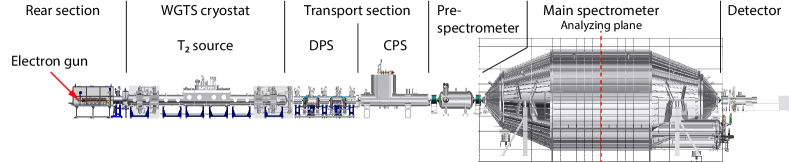
Figure 1: Overview of the KATRIN experiment. The main components are from left to right: The rear section containing calibration and monitoring systems as well as the electron gun (see Fig. 2) used in this work; the $10$-$\mathrm{m}$-long windowless gaseous tritium source (WGTS) with differential pumps on both sides; the transport section consisting of a differential (DPS) and cryogenic pumping section (CPS); the spectrometer and detector section with the pre- and main spectrometer, and the silicon detector. The overall length of the experimental setup is more than $70\text{\,}\mathrm{m}$.

The pre- and main spectrometer are MAC-E type high-pass filters, which can only be traversed by electrons with longitudinal kinetic energy higher than the preset potential. The isotropically emitted $\upbeta$-electrons are adiabatically collimated to a longitudinal motion inside the spectrometer. This is achieved by a gradual decrease of the magnetic field strength $B$ from the entrance of the spectrometer towards its center, conserving the magnitude of the $\upbeta$-electron’s magnetic moment in the cyclotron motion $\mu=E_{\perp}/B$ Beamson1980 , with $E_{\perp}$ being the transverse component of the electron’s kinetic energy with respect to the magnetic field lines. Varying the electric potential of the spectrometer allows the energy region around the endpoint of the tritium $\upbeta$-decay to be scanned as an integral spectrum, i.e. the rate of electrons with kinetic energy above the set filter potential Aker2021 .

Electrons passing the main spectrometer are re-accelerated by the main spectrometer potential and a post-acceleration of $10\text{\,}\mathrm{kV}$ at the focal-plane detector (FPD) system and are then counted by a 148-pixel silicon PIN detector Ams15 shown at the far right in Fig. 1. An $18$-$\mathrm{keV}$-wide selection window ($14\text{\,}\mathrm{keV}$ to $32\text{\,}\mathrm{keV}$) around the $28$-$\mathrm{keV}$ electron energy peak is chosen to minimize systematic effects in counting efficiencies Aker2021 .

The observable $m_{\nu}^{2}$ is determined by fitting the recorded integral spectrum with a model that comprises four parameters: the normalization, the endpoint energy, the background rate, and $m_{\nu}^{2}$ Kleesiek2019 . The model is constructed from the shape of the $\upbeta$-decay spectrum and the response of the experimental setup. The main components of the response are the transmission function of the main spectrometer and the energy loss of electrons from elastic and inelastic scatterings in the T₂ source. The latter is the focus of this work.

At the nominal source density, approximately $60\text{\,}\mathrm{\char 37\relax}$ of all electrons scatter inelastically and lose energies between $\approx\,$$11\text{\,}\mathrm{eV}$ and $9.3\text{\,}\mathrm{keV}$. The upper limit of this energy transfer arises due to the fact that the primary and secondary electrons from the ionization process are indistinguishable in the measurement and always the higher energetic electron is measured. Minuscule energy losses can result in electrons with energies close to the endpoint downgraded to lower energies in the spectrum fit window. Therefore, the energy-loss function needs to be known with high precision in order to meet the systematic uncertainty budget of$\sigma(m_{\nu}^{2})<$7.5\text{\times}{10}^{-3}\text{\,}{\mathrm{eV}}^{2}$$ KAT04 reserved for this individual systematic.

Theoretical differential cross sections for $18.6$-$\mathrm{keV}$ electrons scattering off molecular tritium are not available at the required precision for the $m_{\nu}^{2}$ measurements. While data from energy-loss measurements for gaseous tritium or deuterium from the former neutrino mass experiments in Troitsk and Mainz Ase00 ; Abd17 exist, the precision is not sufficient to achieve the KATRIN design sensitivities. Other more precise experimental data on the energy losses of electrons with energies near the tritium $\upbeta$-decay endpoint energy are only available for molecular hydrogen as the target gas Abd17 ; Gei64 ; Uls72 . In this paper we report the results of the in-situ measurements of the energy-loss function in the KATRIN experiment.

We used a monoenergetic and angular-selective electron gun, of the type described in Beh16 , mounted in the rear section (far left in Fig. 1), which allowed us to probe the response of the entire KATRIN setup, including the energy loss in tritium gas.

We begin this paper in Sec. 2 with a brief introduction to existing energy-loss function models and continue with the description of the novel semi-empirical parametrization developed in this work. In Sec. 3, the measurement approaches of the integral as well as the novel differential time-of-flight measurements are explained, including a description of the working principle of the electron gun used for these measurements. The analysis of the tritium data using a combined fit is presented in Sec. 4 including a detailed discussion of the systematic uncertainties of the measurements. Additional measurement results for the energy-loss function in deuterium gas are provided in Sec. 4.3. We conclude this paper in Sec. 5 by summarizing and discussing our results in the context of the neutrino-mass-sensitivity goal of KATRIN.

2 Energy-loss function

Multiple processes contribute to the energy loss of electrons traversing molecular tritium gas. The median energy loss from elastic scattering amounts to $\overline{\Delta E}_{\mathrm{el}}=$2.3\text{\,}\mathrm{meV}$$ Kleesiek2019 , which is negligible in the KATRIN measurement. The predominant processes for the KATRIN experiment are inelastic scatterings, resulting in electronic excitations in combination with rotational and vibrational excitations of the molecule, ionization, and molecular dissociation.

Data from detailed measurements is only available for the scattering of $25$-$\mathrm{keV}$ electrons on molecular hydrogen gas Gei64 ; Uls72 ; these direct measurements of the energy-loss function were made with energy resolutions down to 40 meV. In these measurements, the contribution of three different groups of lines can be discerned, which are created from the excitations of the $(\mathrm{2p}\sigma\ ^{1}\Sigma^{+}_{\mathrm{u}})$, $(\mathrm{2p}\pi\ ^{1}\Pi_{\mathrm{u}})$, and $(\mathrm{3p}\pi\ ^{1}\Pi_{\mathrm{u}})$ molecular states around $12.6\text{\,}\mathrm{eV}$ and $15\text{\,}\mathrm{eV}$, respectively.

Aseev et al. Ase00 and Abdurashitov et al. Abd17 report on the measurements of energy losses of electrons in gaseous molecular hydrogen, deuterium, and tritium. The shape of the energy-loss function was evaluated by fitting an empirical model to the integral energy spectra obtained with a mono-energetic electron source which generated a beam of electrons with kinetic energies near the endpoint energy of the tritium $\upbeta$-decay. Because of the low energy resolution of several eV, the shape of the energy-loss function was coarsely approximated by a Gaussian to represent electronic excitations and dissociation, and a one-sided Lorentzian to represent the continuum caused by ionization of the molecules Ase00 .

2.1 New Parametrization

The high-quality data from the first KATRIN energy-loss measurements described in Sec. 3 allows us to improve the parametrization used in Aseev et al. Ase00 and Abdurashitov et al. Abd17 . While the experimental energy resolution is not sufficient to resolve individual molecular states, the combined contribution of each of the three groups of states can clearly be discerned in the KATRIN data.

A new parametrization of the energy-loss function was developed to describe the inelastic scattering region between about 11 eV and 15 eV using three Gaussians, each of which is approximating one group of molecular states. The ionization continuum beyond this energy region is described by the relativistic binary-encounter-dipole (BED) model developed by Kim et al. Kim2000 . While the parameters required by this model are only available for the ionization of H₂-molecules Kim94 , by taking into account the ionization thresholds for the different isotopologs Wec99

$$\begin{split}E_{\mathrm{i}}(\mathrm{H}_{2})&=$15.433\text{\,}\mathrm{e}\mathrm{V}$\\ E_{\mathrm{i}}(\mathrm{D}_{2})&=$15.470\text{\,}\mathrm{e}\mathrm{V}$\\ E_{\mathrm{i}}(\mathrm{T}_{2})&=$15.486\text{\,}\mathrm{e}\mathrm{V}$\,,\end{split}$$ (1)

the shape of the BED model is a good representation for the tritium data, as can be seen from the fit result in Sec. 4.1. The new parametrization of the full energy-loss function is written as:

$$f(\Delta E)=\begin{cases}\sum_{j=1}^{3}a_{j}\exp\left(-\frac{(\Delta E-m_{j})^{2}}{2\sigma_{j}^{2}}\right)&:\Delta E\leq E_{\mathrm{i}}\\ \frac{f(E_{\mathrm{i}})}{f_{\rm BED}(E_{\mathrm{i}})}\cdot f_{\rm BED}(\Delta E)&:\Delta E>E_{\mathrm{i}},\end{cases}$$ (2)

where $\Delta E$ is the energy loss and $a_{j}$, $m_{j}$, and $\sigma_{j}$ are the amplitude, the mean, and the width of the three Gaussians, respectively. $f_{\rm BED}(\Delta E)$ is the functional form of the BED model as given in Kim2000 and $E_{\mathrm{i}}$ is the junction point between the two regions given by the ionization threshold. For a smooth continuation of the model at the junction, the BED function $f_{\rm BED}(\Delta E)$ is normalized to the local value $f(E_{\mathrm{i}})$ of the Gaussian components at that position.

3 Measurements

The energy-loss function $f(\Delta E)$ (Eq. 2) describes the electron energy losses $\Delta E$ from scattering inside the source, which distort the shape of the response function. By measuring the response function, it is possible to determine $f(\Delta E)$. For this, a quasi-monoenergetic and angular-selective photoelectron source (“electron gun”), located at the end of the rear section (see Fig. 1), is used. Guiding the quasi-monoenergetic beam — at a pitch angle of approx. $\theta=$0\text{\,}\mathrm{\SIUnitSymbolDegree}$$ between the magnetic field lines and the electrons’ momentum vector — through the WGTS allows the investigation of the energy loss from scatterings with the source gas molecules stabilized at $30\text{\,}\mathrm{K}$. Measuring the electron rate at the focal-plane detector as a function of the electron surplus energy $E_{\mathrm{s}}$ at the analyzing plane (see Eq.  3) yields the response function of the setup.

The working principle of the electron gun and a general description of the measurement strategy are provided in the following. This is followed by a discussion of the measurement data taken in the two different measurement modes (integral and differential) as well as two important systematic effects in the measurements (pile-up and background).

Electron gun

A schematic drawing of the electron gun is provided in Fig. 2. The electrons are generated by photoelectric emission when ultraviolet light is shone through an approximately $30$-$\mathrm{nm}$-thick gold photocathode, which is installed inside two electrically charged parallel plates. The photoelectrons are accelerated by a potential difference of $4\text{\,}\mathrm{kV}$ between the plates separated by $10\text{\,}\mathrm{mm}$; the electrons exit the setup through a hole in the front plate (see Fig. 2). This first non-adiabatic acceleration collimates the beam of photoelectrons in a cosine distribution Pei_2002 initially. By tilting the plates by the angle $\alpha$, well-defined pitch angles $\theta$ can be obtained. A pitch angle of $\theta=$0\text{\,}\mathrm{\SIUnitSymbolDegree}$$, which is reached by aligning the plates with the magnetic field lines, is used in the measurements. The generated electrons are further accelerated by a cascade of cylinder electrodes to the desired kinetic energy. The working principle is explained in more detail in Beh16 . The energy profile of the generated beam depends on the work function $\Phi$ of the photocathode and the wavelength $\lambda$ of the light source.

For the measurements in this work, a $266\text{\,}\mathrm{nm}$ pulsed UV laser with pulse widths of less than $18\text{\,}\mathrm{ns}$ (FWHM) is used. The Q-switch of the laser can be externally triggered, which allows the synchronization of the creation time of the electron pulses with the detector system. This allows the time-of-flight (TOF) of the signal electrons to be measured. The TOF is used for a differential analysis of the data (see Sec. 3.2).

The photon energy of the monochromatic laser light(${h\nu=$4.66\text{\,}\mathrm{eV}$}$) is only $0.22\text{\,}\mathrm{eV}$ above the work function $\Phi=$4.44\text{\,}\mathrm{eV}$$ PhDSack2020 of the gold photocathode, which results in a measured energy spread of $\sigma_{\mathrm{E}}<$90\text{\,}\mathrm{meV}$$.

To generate electrons with well defined kinetic energies close to the tritium endpoint, voltages down to $-21\text{\,}\mathrm{kV}$ can be applied to the photocathode and cylinder electrodes. The photocathode potential $U_{\mathrm{ph}}$ is varied to produce electrons with different surplus energies $E_{\mathrm{s}}$ with respect to the negative main spectrometer retarding potential $U_{0}$:

$$E_{\mathrm{s}} =q\cdot U_{\mathrm{s}}+h\nu-\Phi_{i}=q\cdot\left(U_{\mathrm{ph}}-U_{0}\right)+h\nu-\Phi_{i}\,,$$ (3)

taking into account the additional initial energy of the electrons given by the difference of the photon energy $h\nu$ and the work function $\Phi_{i}$ of the electrons populating different energy levels in the solid (neglecting further solid-state effects). The total initial kinetic energy of the electrons is given as $E_{\mathrm{kin}}=q\cdot U_{\mathrm{ph}}$.

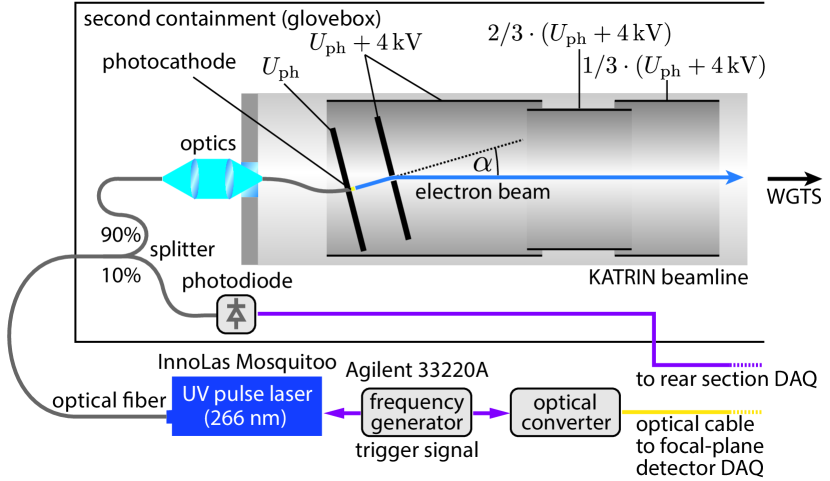
Figure 2: A simplified schematic drawing of the electron gun, including the acceleration electrodes as well as the optical setup used to generate the photoelectrons.

Measurement approach

To resolve the fine structures of the response function, small voltage steps on the order of $0.1\text{\,}\mathrm{eV}$ are required over the analysis interval of $E_{\mathrm{s}}=$$-5\text{\,}\mathrm{eV}60\text{\,}\mathrm{eV}$. Multiple fast voltage sweeps in alternating directions are preferred to compensate for systematic uncertainties associated with the scan direction and long-term instabilities of the setup. A single high-voltage setpoint adjustment of the main spectrometer requires more than $10\text{\,}\mathrm{s}$ to stabilize, which does not allow repeated measurements within a reasonable time. For faster measurements, the surplus energy of the electron beam is modified by performing voltage sweeps of $U_{\mathrm{ph}}$ while the filter potential of the main spectrometer is kept fixed at $U_{0}=-$18575\text{\,}\mathrm{V}$$. The electron energy is chosen to be slightly above the tritium endpoint energy to avoid $\upbeta$-electron backgrounds but close to the region of interest to minimize effects from the energy dependence of the scattering cross section.

Changing the kinetic energy of the electrons results in a small change of the total inelastic scattering cross section $\sigma^{\mathrm{tot}}_{\mathrm{inel}}$ of up to $0.27\text{\,}\mathrm{\char 37\relax}$ over the scanned energy range. This is considered later in the data analysis.

Each sweep (called “scan” in the following) took $30\text{\,}\mathrm{min}$ and was repeated in alternating scanning directions for approximately $12\text{\,}\mathrm{h}$. The obtained rates as a function of the continuous voltage ramp were binned to obtain discrete energy values for the analysis. The data taking was performed in integral and differential modes, which are described in more detail in the following.

3.1 Integral measurements

In the standard KATRIN measurement mode, only electrons with high enough surplus energies to overcome the main spectrometer retarding potential reach the detector. By changing the kinetic energy of the electrons and keeping the retarding potential at a fixed value, the integral response function was measured. A set of integral measurements at three different non-zero column densities as well as one reference measurement at zero column density (see Tab. 1) were performed. The pulse frequency of the laser was set to $100\text{\,}\mathrm{kHz}$, which results in an estimated mean value of 0.05 generated electrons per light pulse.

Table 1: A summary of the number of scans $\Sigma$ performed at different column densities relative to the nominal value $\rho_{0}d$. The corresponding scattering probability $\mu$ is also shown. The average number of counts $<N_{0}>$ per $50$-$\mathrm{mV}$ bin for the unscattered electrons at $E_{s}\in\left[$2\text{\,}\mathrm{eV}$,$10\text{\,}\mathrm{eV}$\right]$ is provided for the integral dataset, as well as the sum of all unscattered electrons $N_{0}$ at $E_{s}\in\left[$-1\text{\,}\mathrm{eV}$,$1\text{\,}\mathrm{eV}$\right]$ for the differential dataset.

Integral
Column density / $\rho_{0}d$	$\mu$	$\Sigma$	$<N_{0}>$
$0\text{\,}\mathrm{\char 37\relax}$	0.00	28	204806
$14\text{\,}\mathrm{\char 37\relax}$	0.25	14	88002
$41\text{\,}\mathrm{\char 37\relax}$	0.75	26	112655
$86\text{\,}\mathrm{\char 37\relax}$	1.56	31	62191
Differential
Column density / $\rho_{0}d$	$\mu$	$\Sigma$	$N_{0}$
$15\text{\,}\mathrm{\char 37\relax}$	0.27	33	565316
$22\text{\,}\mathrm{\char 37\relax}$	0.41	23	380633
$39\text{\,}\mathrm{\char 37\relax}$	0.72	23	267829
$84\text{\,}\mathrm{\char 37\relax}$	1.52	28	154460

The individual scans were both corrected for rate intensity fluctuations and detector pile-up (see Sec. 3.3). The former are caused by fluctuations of the laser intensity, which is stable to $1.2\text{\,}\mathrm{\char 37\relax}\text{\,}{\mathrm{h}}^{-1}$. The light intensity is continuously monitored by a photodiode connected to a fiber splitter, which is installed just before the light is coupled into the vacuum system of the electron gun (see Fig. 2). The light intensity correction is done by dividing the measured FPD rate by the relative deviation of the light intensity to its mean intensity. The precision of the measured light intensity with this monitoring system is $0.4\text{\,}\mathrm{\char 37\relax}$ and is propagated into the uncertainties of the correction. Data from scans at the same column density are accumulated (Fig.  3). The resulting integral response functions are superpositions of $n$-fold scattering functions, as indicated in the figure by arrows above the measurement data.

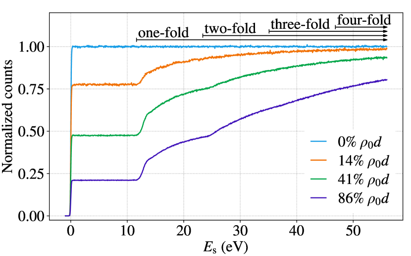
Figure 3: The measured response functions in integral mode at different fractions of the nominal column density $\rho_{0}d$. The response functions are normalized by the electron rate of the reference measurement with an empty source (blue curve). The arrows indicate the energy region where $n$-fold scattering takes place.

3.2 Differential (time-of-flight) measurements

The time of each trigger pulse for the laser is saved in the detector data stream and used to define the electron-emission time at the electron gun. For each event at the detector, its time difference to the laser pulse is calculated. The time difference corresponds to the time-of-flight (TOF) of the electron through the KATRIN beamline from the electron gun to the detector, including delays for the signal propagation and processing on the order of $1\text{\,}\mathrm{\SIUnitSymbolMicro s}$. The knowledge of the electron’s time-of-flight can be used as additional information on its kinetic energy.

The negative retarding potential in the main spectrometer $U_{0}$ acts as a barrier for the electrons, slowing them down and only allowing electrons with surplus energies $E_{\mathrm{s}}>0$ to pass through (high-pass filter). The higher the electrons’ surplus energy, the less they are slowed down inside the main spectrometer; connecting their flight time through the main spectrometer $\tau$ to their surplus energy by $\tau\sim\frac{1}{\sqrt{E_{\mathrm{s}}}}$ Steinbrink2013 .

Selecting only electrons with $\tau>\tau_{\mathrm{cut}}$ is equivalent to a low-pass filter on $E_{\mathrm{s}}$ Bonn1999 . Applying this TOF selection, the high-pass filter main spectrometer is transformed into a narrow band-pass filter for measuring the differential energy spectrum.

For the differential measurements, the laser was pulsed at $20\text{\,}\mathrm{kHz}$ to be able to distinguish flight times up to $50\text{\,}\mathrm{\SIUnitSymbolMicro s}$ between the pulses (see Fig. 4). In this mode, an estimated 0.35 electron per pulse are emitted. Measurements at four different column densities were performed, which are listed in Tab. 1. Figure 4 shows the measurements at $86\text{\,}\mathrm{\char 37\relax}$ nominal column density $\rho_{0}d$ as an example. The top panel shows the time-of-flight versus surplus energy. Here the unscattered electrons as well as one-fold and two-fold scattered electrons are prominently visible as hyperbolic structures.

A TOF selection of events with flight times longer than $\tau_{\mathrm{cut}}=$35\text{\,}\mathrm{\SIUnitSymbolMicro s}$$ is applied to obtain a differential spectrum, which is projected on $E_{\mathrm{s}}$ and shown in the bottom panel. $\tau_{\mathrm{cut}}$ is chosen such that an energy resolution of $\approx\,$$0.02\text{\,}\mathrm{eV}$ is achieved. Higher $\tau_{\mathrm{cut}}$ allows for a higher energy resolution but results in significantly lower statistics. The vertical features — at $0\text{\,}\mathrm{eV}12.5\text{\,}\mathrm{eV}25\text{\,}\mathrm{eV}$ — for ${\tau<$25\text{\,}\mathrm{\SIUnitSymbolMicro s}$}$ are electrons with flight times $>\,$$50\text{\,}\mathrm{\SIUnitSymbolMicro s}$ from a previous laser pulse. These events are neglected in the analysis.

All events with $\tau$ in the range of $35\text{\,}\mathrm{\SIUnitSymbolMicro s}$ to $50\text{\,}\mathrm{\SIUnitSymbolMicro s}$ are selected and corrected for laser intensity fluctuations analogous to the integral analysis. The energy scale for each measurement is constructed using the measured ramping speed of the high voltage and the position of the peak of unscattered electrons set to $E_{\mathrm{s}}=0$.

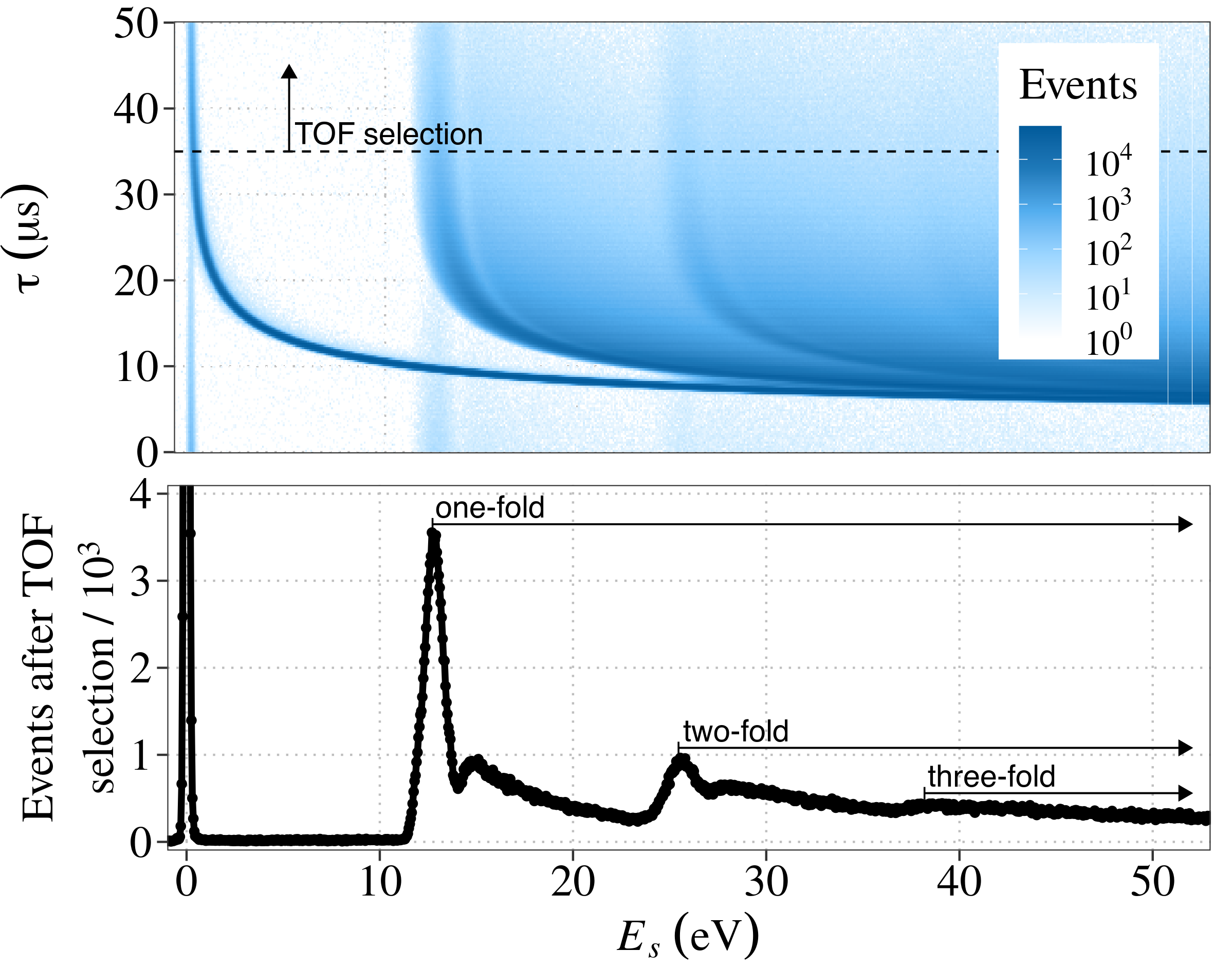
Figure 4: The differential measurements of the time of flight $\tau$ (top) and its one-dimensional projection on the electron surplus energy $E_{\mathrm{s}}$ axis (bottom) at $86\text{\,}\mathrm{\char 37\relax}$ of nominal column density. The dashed line marks the lower boundary of the TOF selection at $\tau_{\mathrm{cut}}=$35\text{\,}\mathrm{\SIUnitSymbolMicro s}$$. The bottom panel shows all events in the TOF selection.

3.3 Pile-up correction

The focal-plane detector is optimized to count single-electron events with an energy resolution of $\Delta E_{\mathrm{FPD}}\approx$2\text{\,}\mathrm{keV}$$. Due to the high electron rate of the electron gun ($\approx\,$${10}^{4}\text{\,}\mathrm{c}\mathrm{p}\mathrm{s}$) and the use of a single detector pixel, pile-up effects become relevant. Furthermore, the pulsed electron beam with $<\,$$18\text{\,}\mathrm{ns}$ FWHM windows creates a non-Poisson time distribution compared to a constant wave light source.

The electron flight time depends on the retarding potential and the energy loss from scatterings inside the WGTS. The time difference of the electrons from the same pulse arriving at the detector is thus modified as a function of the surplus energy. For arrival-time differences shorter than the shaping time ($L=$1.6\text{\,}\mathrm{\SIUnitSymbolMicro s}$$) of the trapezoidal filter used for pulse shaping of the detector signal, the electrons are counted as one single event with correspondingly higher event energy $E_{\mathrm{FPD}}$ (Fig. 5). The number of electrons within the same detector event is denoted as event multiplicity $\mathcal{M}$. As the peaks for different multiplicity $\mathcal{M}$ events overlap in the $E_{\mathrm{FPD}}$ histogram, a simple estimation of $\mathcal{M}$ based on $E_{\mathrm{FPD}}$ is not possible. Processing the event signal with two additional stages of trapezoidal filters allows more information on the signal shape, such as the bipolar width $\mathcal{W}$ (i.e. the time difference of two consecutive zero crossings of the third trapezoidal-filter output), to be obtained Aker2021design . Electrons with arrival-time differences close to the shaping time distort the trapezoidal output of the first filter stage and thus change the determined bipolar width as a function of the arrival-time difference. With the additional information on the pulse shape, these ambiguities can be resolved and $\mathcal{M}$ can be estimated. The multiplicity estimate $\bm{\hat{}}{\mathcal{M}}(E_{\mathrm{FPD}},\mathcal{W})$ is obtained from Monte Carlo simulations of the detector response for random combinations of $\mathcal{M}$ electrons arriving within the shaping time $L$. The estimate $\bm{\hat{}}{\mathcal{M}}(E_{\mathrm{FPD}},\mathcal{W})$ is not necessarily identical to $\mathcal{M}$ as there are still remaining ambiguities, which are considered in the uncertainty propagation (see Sec. 4.2). In the case of the integral measurement data, the correction is made by weighting each event with the estimator value. For the differential measurements, no pile-up correction is required, but a $\bm{\hat{}}{\mathcal{M}}(E_{\mathrm{FPD}},\mathcal{W})>1$ cut is applied for background suppression (see Sec. 3.4).

A comparison of the integral response function before and after pile-up correction is provided in Fig. 6 to demonstrate its dependence on the surplus energy at two different values of $\rho d$. The dependence of $\bm{\hat{}}{\mathcal{M}}(E_{\mathrm{FPD}},\mathcal{W})$ on the kinetic energy of the electrons over the measurement range of $60\text{\,}\mathrm{eV}$ is neglected in the correction and an average estimate is used instead. The uncertainty due to the correction method was evaluated with a full simulation of the detector response for each of the response functions measured in integral mode. This yields a correction stability at $5\text{\times}{10}^{-4}$, which is considered as a systematic uncertainty for the energy-loss function determination.

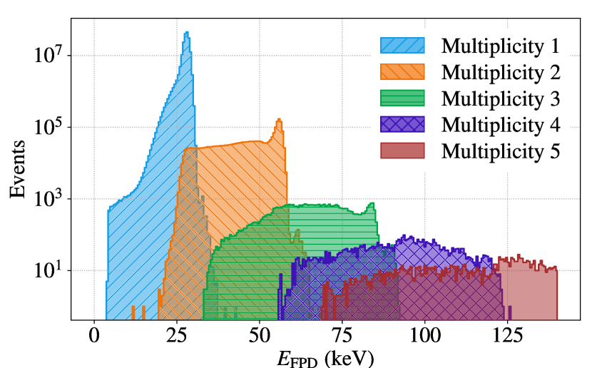
Figure 5: Reconstructed event energy in the focal-plane Si-detector for all events accumulated during the integral response function measurements at $86\text{\,}\mathrm{\char 37\relax}$ nominal column density $\rho_{0}d$. The decomposition with the dedicated pile-up correction method shows that the different multiplicity regions overlap. This effect does not allow for a simple pile-up correction based on event energy alone.

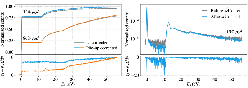
Figure 6: Left: Selection of measured response functions in integral mode before (grey line) and after (colored line) pile-up correction. The correction removes spectral shape distortions up to ten times larger than the statistical uncertainties. Right: Differential response function before and after applying the $\bm{\hat{}}{\mathcal{M}}>1$ cut. The cut reduces the background component by up to a factor of two without significantly influencing the shape of the signal component. Bottom: The difference between the uncorrected/uncut (uc) data and the corrected/cut data normalized to the data point uncertainties $dy$.

3.4 Backgrounds

As the rear section is directly connected to the WGTS, tritium migration upstream towards the electron gun cannot be completely prevented. Tritium can decay within the acceleration fields of the electron gun. Ions created from the $\upbeta$-decays are accelerated towards the photocathode, where their impact can generate multiple secondary electrons simultaneously. Those electrons are accelerated to the same energy as the signal photoelectrons. The kinetic energy of the background electrons changes along with the change of the photocathode voltage $U_{\mathrm{ph}}$ in a scan. This results in a background spectrum following the shape of an integral response function, as it is shown in Fig. 7. The background electrons only differ in their initial energy distribution and the emission multiplicity (i.e. the number of electrons generated from an ion impact). The mean energy $m_{\mathrm{Bg}}$ and the Gaussian width $w_{\mathrm{Bg}}$ of the initial energy distribution of the secondary electrons can be obtained by performing a combined fit to the three background measurements using the same integral response-function model as described in Sec. 4. The initial energy distribution dominates the spectral shape of the transmission function $T(E_{\mathrm{s}})$, which describes the transmission probability of the electrons inside the main spectrometer as a function of the surplus energy $E_{\mathrm{s}}$. The transmission function can be approximated with an error function using $m_{\mathrm{Bg}}$ and $w_{\mathrm{Bg}}$ as free parameters. The nine energy-loss function parameters were fixed to preliminary evaluated values during the fit. The best-fit result yields

$$m_{\mathrm{Bg}}=$2.42(3)\text{\,}\mathrm{eV}$\quad\text{and}\quad w_{\mathrm{Bg}}=$2.05(4)\text{\,}\mathrm{eV}$\,.$$ (4)

The electron multiplicity distribution of the ion-induced events follows a Poisson distribution (including ion-induced events with no electrons being emitted) with the mean value

$$\bm{\hat{}}S=$1.3(4)\text{\,}$\,.$$ (5)

Background events cause a larger detector pile-up effect compared to the signal electrons generated by the pulsed laser, especially in the differential data. The remaining events after the TOF selection are nearly unaffected by detector pile-up, since only the scattered electrons survive. As the arrival time of scattered electrons is delayed compared to other unscattered electrons from the same light pulse, they do not arrive at the detector in time coincidence with other electrons. This allows the multiplicity estimator $\bm{\hat{}}{\mathcal{M}}(E_{\mathrm{FPD}},\mathcal{W})$ to discriminate background events from signal electrons. By excluding events with $\bm{\hat{}}{\mathcal{M}}>1$ in the analysis, the background component can be reduced by about a factor of two without any significant distortion of the signal component. A comparison of the differential response function (at 15% $\rho_{0}d$) before and after applying the multiplicity cut is provided in Fig. 6, showing the reduction of the background component. However, the multiplicity $\bm{\hat{}}{\mathcal{M}}>1$ cut causes a distortion of the shape of the background component, which is determined from simulations. The resulting response functions of the background component after an event multiplicity cut are displayed in Fig. 8. The four simulated spectra of the background components for the individual column densities are included in the fit model.

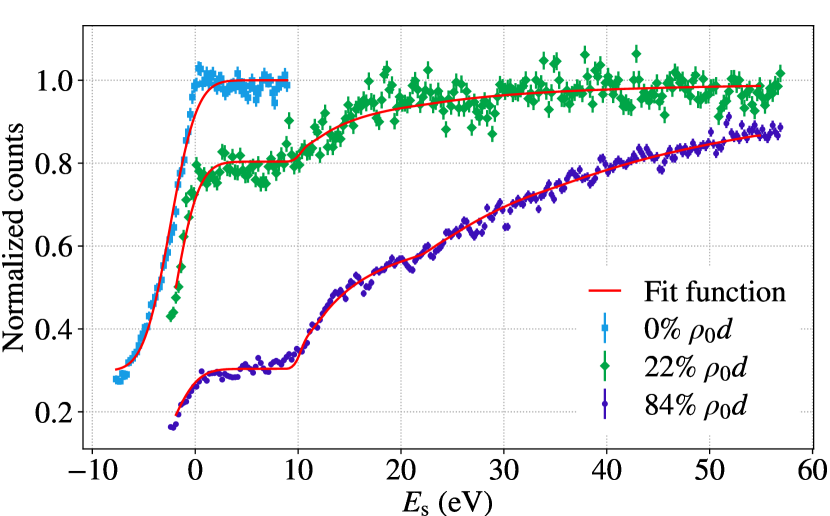
Figure 7: Background measurements of the electron gun with the light source turned off at different fractions of the nominal column density $\rho_{0}d$. Background electrons generated on the emission electrode of the electron gun show similar energy and column density dependencies as signal electrons. Compared to signal electrons, the background energy distribution is broader and shifted towards higher initial values. A combined fit to the data (red line) is used to determine the mean position $m_{\mathrm{Bg}}$ and the width $w_{\mathrm{Bg}}$ of the initial energy distribution. For better illustration, the shown data is normalized such that the region of unscattered electrons in the plateau at $E_{\mathrm{s}}\in\left[$0\text{\,}\mathrm{eV}$,$8\text{\,}\mathrm{eV}$\right]$ equals $P_{0}(\mu)$.

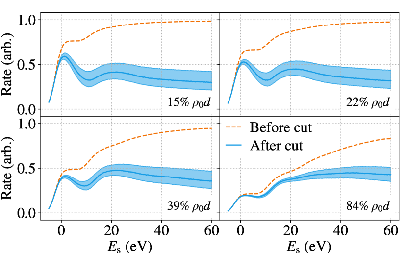
Figure 8: Simulated background spectra with and without multiplicity $\bm{\hat{}}\mathcal{M}>1$ cut for the differential mode after applying the TOF selection. The background spectra without multiplicity cut (orange) show the shape of an integral response function (cf. Fig. 3). The TOF selection (not shown) does not affect this shape of background electrons. The background spectra after multiplicity cut (blue) are strongly reduced but are deformed in shape. The shaded areas show the $1\sigma$ intervals resulting from the uncertainty on the mean emission multiplicity $\bm{\hat{}}S$ of the ion events provided in Eq. (5).

4 Analysis

The energy-loss parameters in Eq. (2) are extracted with a $\chi^{2}$-fit to multiple datasets in integral and differential mode at different column densities. The systematic uncertainties in the energy-loss function (for example, those due to the measurement conditions, pile-up and background effects) are determined with Monte Carlo simulations (cf. Sec. 4.2). Results are given for molecular tritium and deuterium source gases below.

4.1 Combined fit of the datasets

The fit model is constructed with the energy-loss function, effects of multiple scatterings in the source, energy smearing in the experimental setup, and the described background component. The energy-loss function describes a single electron scattering. The probability for $n$-fold scattering follows a Poisson distribution and is given by

$$P_{n}(\mu)=\frac{\mu^{n}}{n!}\exp\left(-\mu\right)\,,$$ (6)

with the expected mean number of scatterings $\mu$ given by

$$\mu=\rho d\cdot\sigma^{\mathrm{tot}}_{\mathrm{inel}}(qU_{0}).$$ (7)

$\rho d$ is the column density during the individual measurements and $\sigma^{\mathrm{tot}}_{\mathrm{inel}}$ is the total inelastic scattering cross section. To correct for the inelastic scattering cross section at different kinetic energies, the parameter $\mu$ is scaled by the ratio ${\sigma^{\mathrm{tot}}_{\mathrm{inel}}(E_{\mathrm{kin}})/\sigma^{\mathrm{tot}}_{\mathrm{inel}}(qU_{0})}$, which gives $P_{n}(\mu,E_{\mathrm{s}})$. The effects of elastic scattering off tritium can be neglected since the amount of energy transferred in these scattering processes (${\overline{\Delta E}_{\mathrm{el}}=$2.3\text{\,}\mathrm{meV}$}$ Kleesiek2019 ) is negligible compared to the energy smearing caused, among others, by the width of the kinetic energy distribution of the electrons produced with the electron gun or the finite energy resolution of the KATRIN main spectrometer. The experimental response to electrons that have been scattered $n$ times in the source gas is given by the $n$-fold convolution of the energy-loss function $f(\Delta E)$ with itself and convolved one time with the experimental transmission function $T(E_{\mathrm{s}})$, leading to the following definition of the corresponding scattering functions $\epsilon_{n}(E_{\mathrm{s}})$

$$\epsilon_{0}(E_{\mathrm{s}})=\; T(E_{\mathrm{s}})\;,$$

$$\epsilon_{1}(E_{\mathrm{s}})=\; T(E_{\mathrm{s}})\otimes f(\Delta E)\;,$$

$$\epsilon_{2}(E_{\mathrm{s}})=\; T(E_{\mathrm{s}})\otimes f(\Delta E)\otimes f(\Delta E)\;,\;...\;,$$ (8)

with $E_{\mathrm{s}}$ being the surplus energy of the electrons (see Eq. (3)) and $\Delta E$ being the energy loss resulting from an inelastic scattering. The shape of the ionization tail of the energy-loss function is corrected for the shape distortion ($<\,$${10}^{-2}\text{\,}\mathrm{\char 37\relax}$) caused by the change of the kinetic energy.

The model $R(E_{\mathrm{s}},\mu)$, which is fit to data, is the sum of the scattering functions $\epsilon_{n}(E_{\mathrm{s}})$ weighted by the corresponding Poissonian probabilities

$$R(E_{\mathrm{s}},\mu)=\sum_{n=0}^{4}P_{n}(\mu,E_{\mathrm{s}})\cdot\epsilon_{n}(E_{\mathrm{s}}).$$ (9)

Given that the surplus energies considered in the energy-loss analysis are limited to ${E_{\mathrm{s}}\leq$56\text{\,}\mathrm{eV}$}$, the highest scattering order that needs to be considered is $n=4$.

In the integral measurement, the shape of the experimental transmission function $T_{\rm int}(E_{\mathrm{s}})$ is obtained from the response function with an empty source volume; Eq. (9) collapses to $R(E_{\mathrm{s}},0)=T(E_{\mathrm{s}})$. $T(E_{\mathrm{s}})$ is modeled with an error function. Similarly, the transmission function for the differential data $T_{\rm dif}(E_{\mathrm{s}})$ could be obtained from a TOF measurement with an empty source. However, it is simply given by the shape of the peak of unscattered electrons observed at non-zero column densities; no additional measurement is required in this case. Thus, we directly use the measurement data to construct the fit model. Figure 9 shows the scattering functions constructed for the differential ($\epsilon_{n}^{\rm dif}(E_{\mathrm{s}})$) and the integral ($\epsilon_{n}^{\rm int}(E_{\mathrm{s}})$) measurement modes for the first four scattering orders.

In addition to the nine parameters in the energy-loss model in Eq. (2) (amplitude, mean and width of the three Gaussians contained in the model), several nuisance parameters are included in the combined fit to differential and integral datasets taken at different column densities. These nuisance parameters include normalization factors $c^{\rm{dif(int)}}_{i}$, mean scattering probabilities $\mu^{{\rm dif(int)}}_{i}$, and background amplitudes $b^{{\rm dif(int)}}_{i}$ for each differential (integral) dataset that is added to the fit. In the fit, we minimize the following $\chi^{2}$ function for the vector of free fit parameters $\vec{\mathcal{P}}$

 

$$\chi^{2}\left(\vec{\mathcal{P}}\right)= \sum_{i}^{N_{\rm dif}}\sum_{j}\left(\frac{c^{{\rm dif}}_{i}\,R^{\rm dif}(E_{\mathrm{s},j},\mu^{{\rm dif}}_{i})+b^{{\rm dif}}_{i}\,B^{\rm dif}(E_{\mathrm{s},j},\mu^{{\rm dif}}_{i})-y^{{\rm dif}}_{i,j}}{dy^{{\rm dif}}_{i,j}}\right)^{2}$$

$$+ \sum_{i}^{N_{\rm int}}\sum_{j}\left(\frac{c^{{\rm int}}_{i}\,R^{\rm int}(E_{\mathrm{s},j},\mu^{{\rm int}}_{i})+b^{{\rm int}}_{i}\,B^{\rm int}(E_{\mathrm{s},j},\mu^{{\rm int}}_{i})-y^{{\rm int}}_{i,j}}{dy^{{\rm int}}_{i,j}}\right)^{2}$$

$$+ \left(\frac{\int^{E_{\mathrm{max}}}_{0}f(\Delta E)d(\Delta E)-1}{\delta}\right)^{2}\;,$$ (10)

 

where $N_{\rm dif(int)}$ are the number of differential (integral) datasets considered. $y^{{\rm dif(int)}}$ and $dy^{{\rm dif(int)}}$ represent the individual data points and their uncertainties. The index of summation $j$ denotes the data points of the individual datasets. The first summand of Eq. (4.1) describes the contribution of the differential datasets to the $\chi^{2}$ value. The fit range for the differential datasets extends from $10\text{\,}\mathrm{eV}$ to $56\text{\,}\mathrm{eV}$, excluding the zero-scatter peak and the adjacent background region, which do not contain information on the energy-loss function. The second summand describes the contribution of integral datasets with the fit range of $-1\text{\,}\mathrm{eV}$ to $56\text{\,}\mathrm{eV}$ . The ion-induced background component (see Sec. 3.4) is considered in both summands. For the integral measurements, the shape of the background component $B^{\rm int}(E_{\mathrm{s},j},\mu^{{\rm int}}_{i})$ is described by an integral response function (see Fig. 7), but with a different initial energy distribution than the signal electrons. For the differential measurement, $B^{\rm dif}(E_{\mathrm{s},j},\mu^{{\rm dif}}_{i})$ is more complex and is obtained from simulations described in Sec. 3.4 and depicted in Fig. 8. The third summand is a pull term that ensures a proper normalization of the fitted energy-loss function up to $E_{\mathrm{max}}=(E-E_{\mathrm{i}})/2$ with a desired precision of $\delta=10^{-4}$.

With the definition of the $\chi^{2}$ given in Eq. (4.1), a combined fit to four differential datasets and three integral datasets taken at different column densities (see Tab. 1) was performed. The results are displayed in Fig. 10 for each of the differential and integral datasets included in the fit.

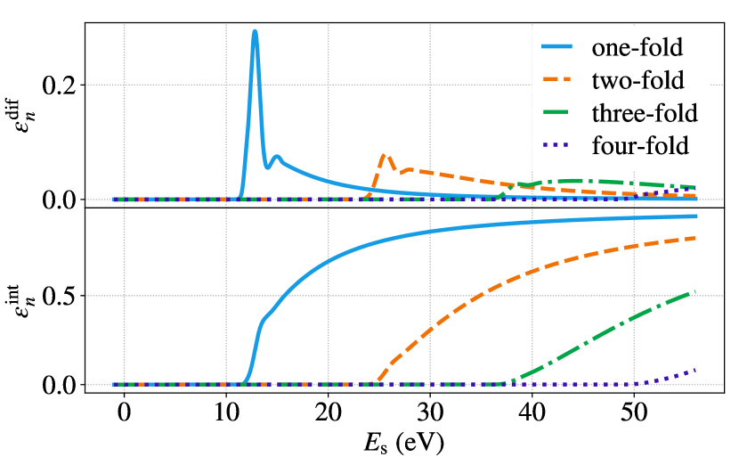
Figure 9: Differential ($\epsilon_{n}^{\mathrm{dif}}(E_{\mathrm{s}})$) and integral ($\epsilon_{n}^{\mathrm{int}}(E_{\mathrm{s}})$) scattering functions for up to four-fold scattering.

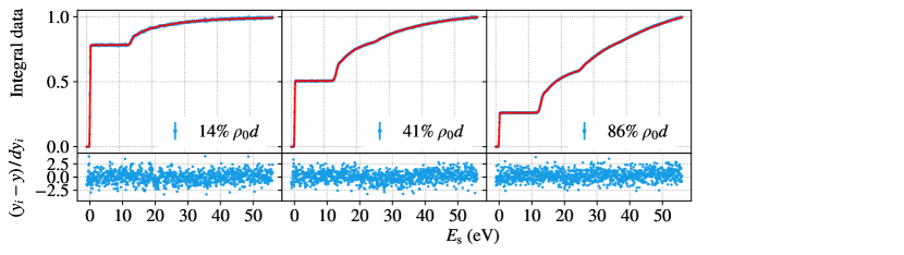
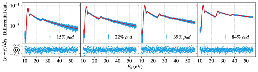
Figure 10: Results of the combined fit to the differential and integral datasets at different column densities. Each panel shows the data points (blue) and the best-fit result (red) in the upper part and the corresponding residuals in the lower part. A normalization is applied to each of the differential and integral response functions. The differential data is normalized by the total number of counts within the fit range and the integral data by the number of counts in the last bin.

The corresponding best-fit parameters of the energy-loss function are given in Tab. 2. The fit has a reduced $\chi^{2}$ value of $1.13(2)\text{\,}$. A deviation from $\chi^{2}/N_{\mathrm{dof}}=1$ can arise from an imperfect semi-empirical parametrization of the energy-loss function or an underestimation of uncertainties. We do not observe significant structures in the fit residuals in Fig. 10 and thus inflate the uncertainties of the data points by $\sqrt{\chi^{2}/N_{\mathrm{dof}}}$ to achieve a $\chi^{2}/N_{\mathrm{dof}}=1$ PDG2020 . The statistical uncertainties from the fit are included in the third column of Tab. 2 with the covariance matrix shown in Tab. 5 in the Appendix. Compared to the empirical energy-loss models of Aseev et al. and Abdurashitov et al. superimposed on our results in Fig. 3, the KATRIN result provides a better energy resolution and reduced uncertainties. As a consistency check, we extrapolate the energy-loss function (fitted up to $56\text{\,}\mathrm{eV}$) to ${E_{\mathrm{max}}=$9.280\text{\,}\mathrm{keV}$}$ yielding a mean energy loss of $\overline{\Delta E}(\mathrm{T}_{2})=30.79(1)_{\mathrm{fit}}$ eV, which agrees well with the value of $29.9(10)\text{\,}\mathrm{eV}$ reported by Aseev et al. Ase00 .

Table 2: Best-fit parameters for the energy-loss function in molecular tritium as described in Eq. (2). Parameter correlations are provided as a covariance matrix in Tab. 5 in the Appendix.

Parameter	Unit	Value
$m_{1}$	$\mathrm{eV}$	$11.9189(83)$
$m_{2}$	$\mathrm{eV}$	$12.8046(21)$
$m_{3}$	$\mathrm{eV}$	$14.9677(41)$
$\sigma_{1}$	$\mathrm{eV}$	$0.1836(70)$
$\sigma_{2}$	$\mathrm{eV}$	$0.4677(22)$
$\sigma_{3}$	$\mathrm{eV}$	$0.907(13)$
$a_{1}$	${\mathrm{eV}}^{-1}$	$0.0328(12)$
$a_{2}$	${\mathrm{eV}}^{-1}$	$0.29570(68)$
$a_{3}$	${\mathrm{eV}}^{-1}$	$0.07575(37)$

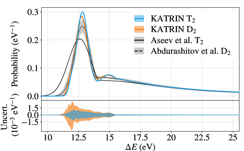
Figure 11: A comparison of the energy-loss functions in D₂ and T₂ from this work and previous measurements of Aseev et al. Ase00 and Abdurashitov et al. Abd17 . The y-axis indicates the probability density normalized in $\Delta E\in\left[0,E_{\mathrm{max}}\right]$ for energy losses $\Delta E$ due to inelastic scattering. The Gaussian $1\sigma$ uncertainty bands are indicated by the shaded areas. Since the uncertainty of the KATRIN T₂ and D₂ results are too small to be visible in the top plot, the uncertainties are additionally shown in absolute values in the bottom plot.

4.2 Systematic uncertainties

Systematic uncertainties are not included in the combined fit; they are determined separately by a Monte Carlo (MC) simulation framework. The framework generates many MC samples, each composed of a detailed simulation of all integral and differential datasets. The systematic effects under investigations can be folded into these MC sets individually, or combined, with or without statistical fluctuation of the count rates included. The underlying response function, on which the MC generation is based, is taken from the best-fit values given in Tab. 2.

The considered systematic uncertainties cover known effects that arise from the measurement conditions and effects specific to the integral or differential analysis. All systematic effects are shown in Tab. 3. Their implementation in MC generation is described in the following.

Table 3: A list of systematic uncertainties. The listed systematics are investigated by MC simulations yielding the contribution to the total parameter uncertainties and the parameter shifts, which are displayed in Fig. 12. The area of the uncertainty band of the energy-loss function caused by the individual systematic effects relative to that of all systematic effects is provided in the second to last column. The resulting parameter shifts due to each systematic effect are quantified in the last column as the area of the absolute deviations of the nominal function and the function given by the parameter means of the systematic variation. See text for more details.

Systematic effect	Source of input	Input values	$\frac{\int|\sigma_{\mathrm{sys}}|}{\int|\sigma_{\mathrm{all}}|}$	$\frac{\int|f_{0}-f_{\mathrm{sys}}|}{\int|\sigma_{\mathrm{all}}|}$
Transmission-function model	error function fit to reference measurement	${m_{\mathrm{E}}=$-0.2(22)\text{\,}\mathrm{meV}$}$ ${w_{\mathrm{E}}=$90(1)\text{\,}\mathrm{meV}$}$	$0.94$	$0.260$
Column-density drift	throughput sensor	$<0.2\text{\,}\mathrm{\char 37\relax}\mathrm{/}\mathrm{h}$ modeling according to sensor data	$0.015$	$0.023$
Rate drift	measurement data	$<0.15\text{\,}\mathrm{\char 37\relax}\mathrm{/}\mathrm{h}$	$0.002$	$0.004$
Background	bg measurement	${m_{\mathrm{Bg}}=$2.42(3)\text{\,}\mathrm{eV}$}$ ${w_{\mathrm{Bg}}=$2.05(4)\text{\,}\mathrm{eV}$}$	$0.032$	$0.008$
Multiplicity cut	bg measurement and simulation	${\bm{\hat{}}S=$1.3(4)\text{\,}$}$	$0.153$	$0.327$
Pile-up correction	simulation	max. $0.05\text{\,}\mathrm{\char 37\relax}$	$0.166$	$0.271$
Binning	HV sweep	bin width of $0.05\text{\,}\mathrm{eV}$	$0.0$	$0.110$
All systematics			$1.0$	$0.395$

• Transmission-function model In order to obtain an analytical description of the integral transmission function $T(E_{\mathrm{s}})$ for the construction of the integral response-function model, an error function is fit to a reference measurement with an empty WGTS. The error function models the electron’s surplus energy threshold needed for transmission in the main spectrometer $m_{\mathrm{E}}=$-0.2(29)\text{\,}\mathrm{meV}$$ and the energy spread $w_{\mathrm{E}}=$90(2)\text{\,}{\mathrm{m}\mathrm{eV}}$$ due to the angular and energy distribution of the electron gun and the energy resolution of the main spectrometer. To investigate the uncertainty of this analytical model, MC samples of the measurements at different column densities were generated with $m_{\mathrm{E}}$ and $w_{\mathrm{E}}$ drawn from a multivariate normal distribution according to the best-fit values above with the correlation between them taken into account. No uncertainty on the transmission-function model was considered for the differential data, since the peak of the unscattered electrons from the measurement data is directly used as the transmission function.

• Column-density drift As the scattering probability $P_{n}$ depends on the column density, drifts in the column density during the measurements can cause a distortion of the response function. During the measurements at $41\text{\,}\mathrm{\char 37\relax}$ of the nominal column density, drifts on the order of $0.2\text{\,}\mathrm{\char 37\relax}\mathrm{/}\mathrm{h}$ were visible. The reduced stability was caused by CO and tritiated methane freezing inside the injection capillaries. The CO and the methane were generated from radiochemical reactions with the stainless-steel surface during the burn-in period of the first tritium operation Aker2021 . The column density is constantly monitored with a throughput sensor, which allows the drift to be modeled precisely in the simulations. To do so, a linear function $\rho(t)$ is fit to the sensor data, yielding the slope of the drift and the corresponding parameter uncertainty. This linear function is used to model the rate drift due to the column density drift with the slope sampled according to its uncertainty.

• Rate drift The electron-production rate of the electron gun can drift due to changes in the work function or a possible degradation of the photocathode (e.g. by ion impacts). The number of unscattered electrons is analyzed for each run after correcting for drifts in the light intensity and the column density to monitor for intrinsic long-term rate drifts. Although the rate drift is very small at $\mathcal{O}($0.1\text{\,}\mathrm{\char 37\relax}\text{\,}{\mathrm{h}}^{-1}$)$, the resulting drift is used to modulate the response functions accordingly.

• Background A background component created from secondary electrons by ion impact on the photocathode (cf. Sec. 3.4) adds to the response functions. In the MC simulations, a background component is added with the parameters of the initial energy distribution of the background electrons (see Eq. (4)) sampled according to their uncertainties.

• Multiplicity cut The event multiplicity ${\bm{\hat{}}{\mathcal{M}}(E_{\mathrm{FPD}},w)>1}$ cut distorts the background shape in the differential measurements (see Fig. 8) depending on the initial electron multiplicity $\bm{\hat{}}S$ (see Eq. (5)) of the ion impact. In the MC simulations, the value of $\bm{\hat{}}S$ is sampled according to its Gaussian uncertainty determined from the measurement and the resulting background component is added to the differential data. Distortions on the signal component from the photoelectrons due to the multiplicity cut were investigated by dedicated detector simulations and added to the differential response functions.

• Pile-up correction Detector pile-up is a dominant systematic effect for the integral measurements and is corrected with the pile-up reconstruction method described in Sec. 3.3. The efficiency $\zeta(E_{s})$ of this pile-up correction method is determined with detector simulations for each data point. The simulated response functions are multiplied by $\zeta(E_{s})$ to include the remaining distortions after applying the pile-up correction. The efficiency $\zeta(E_{s})$ is varied according to the Gaussian uncertainty determined in detector simulations.

• Binning The response functions are measured by continuously ramping the emission energy of the electron gun. For the data analysis, the continuous data stream is binned into $50$-$\mathrm{meV}$ bins. This binning effect is included in the MC simulations.

A total of 10000 MC datasets are generated from the distributions of the systematic effects. Every MC dataset is fit and the best-fit values are taken to construct the probability distribution for each of the nine parameters of interest. From these distributions, the parameter uncertainties are determined from the standard deviations. In addition, systematic parameter shifts are determined from the difference between the median of the distribution and the initial input value from the underlying energy-loss function. The results of this evaluation are shown in Fig. 12. The total uncertainty is dominated by the statistics in the data and the widths of the distributions agree well with the parameter uncertainties of the best-fit result provided in Tab. 2. In order to condense the information of the nine parameter uncertainties for easier interpretation, two metrics are defined. They are shown in the last two columns of Tab. 3. The first metric, $\int|\sigma_{\mathrm{sys}}|/\int|\sigma_{\mathrm{all}}|$, is the area of the error band in the energy-loss function caused by the specific systematic ($\int|\sigma_{\mathrm{sys}}|$) with respect to the area of the error band caused by all systematic effects ($\int|\sigma_{\mathrm{all}}|$). The error bands originate from the combination of all nine parameter uncertainties. The areas of the error bands are estimates for the uncertainty of the scattering probability over the whole energy range. The second metric, $\int|f_{0}-f_{\mathrm{sys}}|/\int|\sigma_{\mathrm{all}}|$, is the area of the difference between the nominal energy-loss function ($f_{0}$) and the energy-loss function ($f_{\mathrm{sys}}$) obtained from the simulations including the individual systematic uncertainties. This difference is normalized to $\int|\sigma_{\mathrm{all}}|$. A difference can be created by shifts of the nine parameter values caused by a given systematic effect. The impact of parameter shifts on the functional form of the energy loss is found to be smaller than the impact of the parameter uncertainties. The dominant contribution to the systematic uncertainty originates from the transmission-function model. Since the total uncertainty of the energy-loss function is dominated by statistical uncertainties in the data and no significant parameter shifts are found, the considered systematic effects are negligible and not further considered in this study.

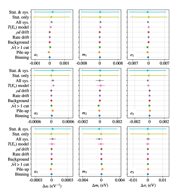
Figure 12: A breakdown of systematic uncertainties for all nine individual energy loss parameters as obtained from Monte Carlo simulations. Shown are the total uncertainty (stat. & sys.), the statistical uncertainty (stat. only) as well as the total systematic uncertainty (all sys.). The data points indicate the difference between the fit to data without any systematic effects and the median of the parameter distribution obtained from the fits to 10000 MC samples with systematic effects. The bars indicate the standard deviation of the distributions. The measurement is strongly dominated by the statistical uncertainty. The investigated systematic effects do not significantly contribute to a broadening of the parameter uncertainties nor to a significant shift of their mean values.

4.3 Deuterium results

Measurements, similar to the ones described in Sec. 3, were performed with molecular deuterium as source gas in an early commissioning run of the KATRIN experiment. Four integral measurements at $0\text{\,}\mathrm{\char 37\relax}5\text{\,}\mathrm{\char 37\relax}35\text{\,}\mathrm{\char 37\relax}87\text{\,}\mathrm{\char 37\relax}$ of the nominal source density and a single differential measurement at $5\text{\,}\mathrm{\char 37\relax}$ were made. The data were processed and fit in the same manner as described in Secs. 3 and 4. For the combined $\chi^{2}$-fit of the deuterium measurements, the best-fit result is obtained at a reduced $\chi^{2}=$1.57(2)\text{\,}$$. Similar to the tritium data, the uncertainties of the data points are rescaled by $\sqrt{\chi^{2}/N_{\mathrm{dof}}}$ to obtain a reduced $\chi^{2}=1$. The parameter values as well as the covariance matrix are provided in Tabs. 4 and 6. The slightly increased $\chi^{2}$ value and the larger model uncertainties (cf. Fig. 3) can be explained by the presence of a stronger detector pile-up in the integral data due to an electron rate that was twice as high as that of the tritium measurements combined with the availability of only one differential dataset. A full propagation of the systematic uncertainties was not performed for the deuterium measurements as the simulations for tritium showed that the measurements are strongly dominated by the statistical uncertainty. Furthermore, neither the systematic uncertainty due to methane freezing causing column-density drift nor the background generated from tritium ions is present in the absence of tritium.

Figure 3 shows the minor differences of the energy-loss models for deuterium and tritium, as the electronic excitation states are shifted to lower energies on the order of $100\text{\,}\mathrm{meV}$ . Extrapolating again to $E_{\mathrm{max}}$ the energy loss function results in a mean energy loss of$\overline{\Delta E}(\mathrm{D}_{2})=30.64(1)_{\mathrm{fit}}$ eV, for the dominant deuterium isotopologs. This mean energy-loss value is $0.15\text{\,}\mathrm{eV}$ smaller than for tritium isotopologs, but we should not forget that we extrapolate the energy-loss function in energy by a factor 200 and we do not account for systematic uncertainties here for this consistency check.

Table 4: Best-fit parameter values for the energy-loss function in molecular deuterium as described in Eq. (2). Parameter correlations are provided as a covariance matrix in Tab. 6.

Parameter	Unit	Value
$m_{1}$	eV	$11.793(20)$
$m_{2}$	eV	$12.7300(46)$
$m_{3}$	eV	$14.875(11)$
$\sigma_{1}$	eV	$0.166(17)$
$\sigma_{2}$	eV	$0.4828(53)$
$\sigma_{3}$	eV	$1.073(32)$
$a_{1}$	${\mathrm{eV}}^{-1}$	$0.0344(28)$
$a_{2}$	${\mathrm{eV}}^{-1}$	$0.2737(15)$
$a_{3}$	${\mathrm{eV}}^{-1}$	$0.07466(47)$

5 Summary and Outlook

A series of precision measurements of the energy-loss function of $18.6$-$\mathrm{keV}$ electrons scattering off molecular tritium and deuterium gas was performed. The measurements were carried out in the KATRIN setup by using a pulsed beam of monoenergetic and angular selected electrons from a photoelectron source. The measurements were made in integral and differential time-of-flight measurement modes.

A new semi-empirical parametrization of the energy-loss function was developed, which describes the set of electronic states in combination with molecular excitations, dissociation, and ionization better than previous models. This new model is described by nine parameters, which were determined by performing a combined $\chi^{2}$-fit to both integral and differential measurement data. The measurements and analyses performed in this work achieved a significant improvement over existing empirical energy-loss models in terms of energy resolution and uncertainties. A detailed investigation of the systematic effects shows that the parameter uncertainties are dominated by statistical uncertainties. This allows further improvement in precision in future measurements.

The obtained electron energy-loss function in tritium was used in the analysis of the first KATRIN dataset, which led to an improved upper limit of the effective neutrino mass ${m_{\nu}<$1.1\text{\,}\mathrm{eV}$}$ (90% C.L.) Aker2019 . For this dataset, recorded at reduced source strength, the uncertainty of the energy-loss model contributes to the systematic uncertainty of the observable $m_{\nu}^{2}$ with $\sigma(m_{\nu}^{2})<${10}^{-2}\text{\,}\mathrm{eV}^{2}$$ and is inconsequential compared to other effects Aker2021 . The achieved precision of the energy-loss function is close to the target effect of ${\sigma(m_{\nu}^{2})<$7.5\text{\times}{10}^{-3}\text{\,}\mathrm{eV}^{2}$}$ KAT04 that is necessary for reaching the final KATRIN sensitivity of ${m_{\nu}=$0.2\text{\,}\mathrm{eV}$}$ (90% CL).

Appendix

Table 5: Covariance matrix for the parametrization of the energy-loss function for molecular tritium, as provided in Tab. 2.

	$m_{1}$	$m_{2}$	$m_{3}$	$\sigma_{1}$	$\sigma_{2}$	$\sigma_{3}$	$a_{1}$	$a_{2}$	$a_{3}$
$m_{1}$	6.941$\cdot$10${}^{\text{-5}}$	1.034$\cdot$10${}^{\text{-5}}$	-3.388$\cdot$10${}^{\text{-6}}$	4.537$\cdot$10${}^{\text{-5}}$	-7.980$\cdot$10${}^{\text{-6}}$	8.094$\cdot$10${}^{\text{-6}}$	4.529$\cdot$10${}^{\text{-6}}$	-6.505$\cdot$10${}^{\text{-7}}$	-6.581$\cdot$10${}^{\text{-8}}$
$m_{2}$	1.034$\cdot$10${}^{\text{-5}}$	4.503$\cdot$10${}^{\text{-6}}$	7.403$\cdot$10${}^{\text{-7}}$	8.265$\cdot$10${}^{\text{-6}}$	-1.206$\cdot$10${}^{\text{-6}}$	-8.627$\cdot$10${}^{\text{-6}}$	1.342$\cdot$10${}^{\text{-6}}$	2.262$\cdot$10${}^{\text{-7}}$	1.893$\cdot$10${}^{\text{-7}}$
$m_{3}$	-3.388$\cdot$10${}^{\text{-6}}$	7.403$\cdot$10${}^{\text{-7}}$	1.641$\cdot$10${}^{\text{-5}}$	-4.727$\cdot$10${}^{\text{-6}}$	3.464$\cdot$10${}^{\text{-6}}$	-2.255$\cdot$10${}^{\text{-6}}$	-1.004$\cdot$10${}^{\text{-6}}$	-1.272$\cdot$10${}^{\text{-7}}$	-6.165$\cdot$10${}^{\text{-7}}$
$\sigma_{1}$	4.537$\cdot$10${}^{\text{-5}}$	8.265$\cdot$10${}^{\text{-6}}$	-4.727$\cdot$10${}^{\text{-6}}$	4.858$\cdot$10${}^{\text{-5}}$	-8.929$\cdot$10${}^{\text{-6}}$	1.503$\cdot$10${}^{\text{-5}}$	2.481$\cdot$10${}^{\text{-6}}$	-9.888$\cdot$10${}^{\text{-9}}$	-1.840$\cdot$10${}^{\text{-7}}$
$\sigma_{2}$	-7.980$\cdot$10${}^{\text{-6}}$	-1.206$\cdot$10${}^{\text{-6}}$	3.464$\cdot$10${}^{\text{-6}}$	-8.929$\cdot$10${}^{\text{-6}}$	4.746$\cdot$10${}^{\text{-6}}$	-1.521$\cdot$10${}^{\text{-5}}$	-1.755$\cdot$10${}^{\text{-6}}$	-5.149$\cdot$10${}^{\text{-7}}$	2.435$\cdot$10${}^{\text{-7}}$
$\sigma_{3}$	8.094$\cdot$10${}^{\text{-6}}$	-8.627$\cdot$10${}^{\text{-6}}$	-2.255$\cdot$10${}^{\text{-6}}$	1.503$\cdot$10${}^{\text{-5}}$	-1.521$\cdot$10${}^{\text{-5}}$	1.632$\cdot$10${}^{\text{-4}}$	3.346$\cdot$10${}^{\text{-6}}$	-2.017$\cdot$10${}^{\text{-6}}$	-4.154$\cdot$10${}^{\text{-6}}$
$a_{1}$	4.529$\cdot$10${}^{\text{-6}}$	1.342$\cdot$10${}^{\text{-6}}$	-1.004$\cdot$10${}^{\text{-6}}$	2.481$\cdot$10${}^{\text{-6}}$	-1.755$\cdot$10${}^{\text{-6}}$	3.346$\cdot$10${}^{\text{-6}}$	1.462$\cdot$10${}^{\text{-6}}$	9.769$\cdot$10${}^{\text{-8}}$	-4.513$\cdot$10${}^{\text{-8}}$
$a_{2}$	-6.505$\cdot$10${}^{\text{-7}}$	2.262$\cdot$10${}^{\text{-7}}$	-1.272$\cdot$10${}^{\text{-7}}$	-9.888$\cdot$10${}^{\text{-9}}$	-5.149$\cdot$10${}^{\text{-7}}$	-2.017$\cdot$10${}^{\text{-6}}$	9.769$\cdot$10${}^{\text{-8}}$	4.581$\cdot$10${}^{\text{-7}}$	4.877$\cdot$10${}^{\text{-8}}$
$a_{3}$	-6.581$\cdot$10${}^{\text{-8}}$	1.893$\cdot$10${}^{\text{-7}}$	-6.165$\cdot$10${}^{\text{-7}}$	-1.840$\cdot$10${}^{\text{-7}}$	2.435$\cdot$10${}^{\text{-7}}$	-4.154$\cdot$10${}^{\text{-6}}$	-4.513$\cdot$10${}^{\text{-8}}$	4.877$\cdot$10${}^{\text{-8}}$	1.354$\cdot$10${}^{\text{-7}}$

Table 6: Covariance matrix for the parametrization of the energy-loss function for molecular deuterium, as provided in Tab. 4.

	$m_{1}$	$m_{2}$	$m_{3}$	$\sigma_{1}$	$\sigma_{2}$	$\sigma_{3}$	$a_{1}$	$a_{2}$	$a_{3}$
$m_{1}$	3.883$\cdot$10${}^{\text{-4}}$	5.087$\cdot$10${}^{\text{-5}}$	-2.607$\cdot$10${}^{\text{-5}}$	2.487$\cdot$10${}^{\text{-4}}$	-4.157$\cdot$10${}^{\text{-5}}$	6.592$\cdot$10${}^{\text{-5}}$	1.214$\cdot$10${}^{\text{-5}}$	-4.525$\cdot$10${}^{\text{-6}}$	-3.856$\cdot$10${}^{\text{-7}}$
$m_{2}$	5.087$\cdot$10${}^{\text{-5}}$	2.093$\cdot$10${}^{\text{-5}}$	1.873$\cdot$10${}^{\text{-5}}$	4.040$\cdot$10${}^{\text{-5}}$	-2.989$\cdot$10${}^{\text{-6}}$	-5.680$\cdot$10${}^{\text{-5}}$	4.437$\cdot$10${}^{\text{-6}}$	2.116$\cdot$10${}^{\text{-6}}$	4.871$\cdot$10${}^{\text{-7}}$
$m_{3}$	-2.607$\cdot$10${}^{\text{-5}}$	1.873$\cdot$10${}^{\text{-5}}$	1.144$\cdot$10${}^{\text{-4}}$	-3.436$\cdot$10${}^{\text{-5}}$	4.237$\cdot$10${}^{\text{-5}}$	-2.466$\cdot$10${}^{\text{-4}}$	-8.612$\cdot$10${}^{\text{-6}}$	5.337$\cdot$10${}^{\text{-6}}$	9.459$\cdot$10${}^{\text{-7}}$
$\sigma_{1}$	2.487$\cdot$10${}^{\text{-4}}$	4.040$\cdot$10${}^{\text{-5}}$	-3.436$\cdot$10${}^{\text{-5}}$	2.793$\cdot$10${}^{\text{-4}}$	-4.330$\cdot$10${}^{\text{-5}}$	6.404$\cdot$10${}^{\text{-5}}$	-4.041$\cdot$10${}^{\text{-6}}$	-7.999$\cdot$10${}^{\text{-7}}$	-5.273$\cdot$10${}^{\text{-8}}$
$\sigma_{2}$	-4.157$\cdot$10${}^{\text{-5}}$	-2.989$\cdot$10${}^{\text{-6}}$	4.237$\cdot$10${}^{\text{-5}}$	-4.330$\cdot$10${}^{\text{-5}}$	2.798$\cdot$10${}^{\text{-5}}$	-1.050$\cdot$10${}^{\text{-4}}$	-7.907$\cdot$10${}^{\text{-6}}$	-2.660$\cdot$10${}^{\text{-7}}$	6.033$\cdot$10${}^{\text{-7}}$
$\sigma_{3}$	6.592$\cdot$10${}^{\text{-5}}$	-5.680$\cdot$10${}^{\text{-5}}$	-2.466$\cdot$10${}^{\text{-4}}$	6.404$\cdot$10${}^{\text{-5}}$	-1.050$\cdot$10${}^{\text{-4}}$	1.033$\cdot$10${}^{\text{-3}}$	1.829$\cdot$10${}^{\text{-5}}$	-2.974$\cdot$10${}^{\text{-5}}$	-1.231$\cdot$10${}^{\text{-5}}$
$a_{1}$	1.214$\cdot$10${}^{\text{-5}}$	4.437$\cdot$10${}^{\text{-6}}$	-8.612$\cdot$10${}^{\text{-6}}$	-4.041$\cdot$10${}^{\text{-6}}$	-7.907$\cdot$10${}^{\text{-6}}$	1.829$\cdot$10${}^{\text{-5}}$	7.761$\cdot$10${}^{\text{-6}}$	2.777$\cdot$10${}^{\text{-7}}$	-6.118$\cdot$10${}^{\text{-8}}$
$a_{2}$	-4.525$\cdot$10${}^{\text{-6}}$	2.116$\cdot$10${}^{\text{-6}}$	5.337$\cdot$10${}^{\text{-6}}$	-7.999$\cdot$10${}^{\text{-7}}$	-2.660$\cdot$10${}^{\text{-7}}$	-2.974$\cdot$10${}^{\text{-5}}$	2.777$\cdot$10${}^{\text{-7}}$	2.173$\cdot$10${}^{\text{-6}}$	4.225$\cdot$10${}^{\text{-7}}$
$a_{3}$	-3.856$\cdot$10${}^{\text{-7}}$	4.871$\cdot$10${}^{\text{-7}}$	9.459$\cdot$10${}^{\text{-7}}$	-5.273$\cdot$10${}^{\text{-8}}$	6.033$\cdot$10${}^{\text{-7}}$	-1.231$\cdot$10${}^{\text{-5}}$	-6.118$\cdot$10${}^{\text{-8}}$	4.225$\cdot$10${}^{\text{-7}}$	2.193$\cdot$10${}^{\text{-7}}$

References

- (1) M. Aker, et al. Analysis methods for the first KATRIN neutrino-mass measurement (2021)
- (2) The KATRIN collaboration, KATRIN design report. FZKA scientific report 7090 (2005). DOI 10.5445/IR/270060419
- (3) M. Aker, et al. The design, construction, and commissioning of the KATRIN experiment (2021). URL https://arxiv.org/abs/2103.04755
- (4) G. Beamson, H. Porter, D. Turner, J. Phys. E: Sci. Instrum. 13(1), 64 (1980). DOI 10.1088/0022-3735/13/1/018
- (5) V. Lobashev, P. Spivak, Nucl. Instrum. Meth. A 240(2), 305 (1985). DOI 10.1016/0168-9002(85)90640-0
- (6) A. Picard, et al., Nucl. Instrum. Meth. B 63(3), 345 (1992). DOI 10.1016/0168-583x(92)95119-c
- (7) F. Friedel, et al., Vacuum 159, 161 (2019). DOI 10.1016/j.vacuum.2018.10.002
- (8) A. Marsteller, B. Bornschein, et al., Vacuum 184, 109979 (2021). DOI 10.1016/j.vacuum.2020.109979
- (9) C. Röttele, J. Phys. Conf. Ser. 888, 012228 (2017). DOI 10.1088/1742-6596/888/1/012228
- (10) J. Amsbaugh, et al., Nucl. Instrum. Meth. A 778, 40 (2015). DOI 10.1016/j.nima.2014.12.116
- (11) M. Kleesiek, et al., Eur. Phys. J. C 79(3) (2019). DOI 10.1140/epjc/s10052-019-6686-7
- (12) V.N. Aseev, et al., Eur. Phys. J. D 10(1), 39 (2000). DOI 10.1007/s100530050525
- (13) D.N. Abdurashitov, et al., Phys. Part. Nuclei Lett. 14(6), 892 (2017). DOI 10.1134/s1547477117060024
- (14) J. Geiger, Z. Physik 181(4), 413 (1964). DOI 10.1007/bf01380873
- (15) R.C. Ulsh, et al., J. Chem. Phys. 60(1), 103 (1974). DOI 10.1063/1.1680755
- (16) J. Behrens, et al., Eur. Phys. J. C 77(6) (2017). DOI 10.1140/epjc/s10052-017-4972-9
- (17) Y.K. Kim, et al., Phys. Rev. A 62(5) (2000). DOI 10.1103/physreva.62.052710
- (18) Y.K. Kim, M.E. Rudd, Phys. Rev. A 50(5), 3954 (1994). DOI 10.1103/PhysRevA.50.3954
- (19) P. Weck, et al., Phys. Rev. A 60(4), 3013 (1999). DOI 10.1103/PhysRevA.60.3013
- (20) Z. Pei, C.N. Berglund, Jpn. J. Appl. Phys. 41(Part 2, No. 1A/B), L52 (2002). DOI 10.1143/jjap.41.l52
- (21) R. Sack, Measurement of the energy loss of 18.6 keV electrons on deuterium gas and determination of the tritium Q-value at the KATRIN experiment. Ph.D. thesis, Westfälische Wilhelms-Universität Münster (2020). URL http://nbn-resolving.de/urn:nbn:de:hbz:6-59069498754
- (22) N. Steinbrink, et al., New J. Phys. 15(11), 113020 (2013). DOI 10.1088/1367-2630/15/11/113020
- (23) J. Bonn, et al., Nucl. Instrum. Meth. A 421(1), 256 (1999). DOI 10.1016/S0168-9002(98)01263-7
- (24) P. Zyla, et al., Prog. Theor. Exp. Phys. 2020(8) (2020). DOI 10.1093/ptep/ptaa104
- (25) A. El Miniawy, A. Saenz. private communication; to be published in the Bachelor thesis of A. El Miniawy (2021)
- (26) M. Aker, et al., Phys. Rev. Lett. 123(22) (2019). DOI 10.1103/physrevlett.123.221802