Massless Preheating and Electroweak Vacuum Metastability

Abstract

Current measurements of Standard Model parameters suggest that the electroweak vacuum is metastable. This metastability has important cosmological implications because large fluctuations in the Higgs field could trigger vacuum decay in the early universe. For the false vacuum to survive, interactions which stabilize the Higgs during inflation—e.g., inflaton-Higgs interactions or non-minimal couplings to gravity—are typically necessary. However, the post-inflationary preheating dynamics of these same interactions could also trigger vacuum decay, thereby recreating the problem we sought to avoid. This dynamics is often assumed catastrophic for models exhibiting scale invariance, since these generically allow for unimpeded growth of fluctuations. In this paper, we examine the dynamics of such “massless preheating” scenarios and show that the competing threats to metastability can nonetheless be balanced to ensure viability. We find that fully accounting for both the backreaction from particle production and the effects of perturbative decays reveals a large number of disjoint “islands of (meta)stability” over the parameter space of couplings. Ultimately, the interplay among Higgs-stabilizing interactions plays a significant role, leading to a sequence of dynamical phases that effectively extend the metastable regions to large Higgs-curvature couplings.

I Introduction

A remarkable implication of the currently measured Standard Model (SM) parameters is that the electroweak vacuum is metastable. Specifically, given the measured Higgs boson and top quark masses Zyla et al. (2020), one finds that at energy scales exceeding $\mu\approx 10^{10}\,\text{GeV}$ the Higgs four-point coupling runs to negative values $\lambda_{h}(\mu)<0$, signifying the existence of a lower-energy vacuum Degrassi et al. (2012); Bezrukov et al. (2012); Alekhin et al. (2012); Buttazzo et al. (2013); Bednyakov et al. (2015). Although today the timescale for vacuum decay is much longer than the age of the universe Andreassen et al. (2018); Chigusa et al. (2018), dynamics earlier in the cosmological history could have significantly threatened destabilization. That the false vacuum has persisted until the present day may thus provide a window into early-universe dynamics involving the Higgs Markkanen et al. (2018).

In this respect, the evolution of the Higgs field during inflation is especially relevant. During inflation, light scalar fields develop fluctuations proportional to the Hubble scale $H$. Without some additional stabilizing interactions, the fluctuations of the Higgs would likewise grow and inevitably trigger decay of the false vacuum, unless the energy scale of inflation is sufficiently small East et al. (2017); Markkanen et al. (2018); Fumagalli et al. (2020).

Metastability thus provides a strong motivation for investigating non-SM interactions that could stabilize the Higgs during inflation—e.g., non-minimal gravitational couplings Espinosa et al. (2008), direct Higgs-inflaton interactions Lebedev and Westphal (2013), etc. However, the situation is actually more delicate, as one must also ensure metastability throughout the remaining cosmological history. While interactions such as those listed above may stabilize the vacuum during inflation, they often proceed to destabilize it during the post-inflationary preheating epoch, thereby recreating the problem we sought to avoid. Indeed, a balancing is typically necessary between the destabilizing effects of inflationary and post-inflationary dynamics.

To this end, a detailed understanding of the field dynamics after inflation is essential in determining which interactions and couplings are well motivated overall. A decisive component of this analysis is the form of the inflaton potential $V(\phi)$ during preheating. After inflation, the inflaton field $\phi$ oscillates coherently about the minimum of its potential. These oscillations determine the properties of the background cosmology, but they also furnish the quantum fluctuations of the Higgs field with time-dependent, oscillatory effective masses. These modulations are the underlying mechanism for Higgs particle production, as they ultimately give rise to non-perturbative processes such as tachyonic instabilities Felder et al. (2001a, b); Dufaux et al. (2006) and parametric resonances Kofman et al. (1994, 1997); Greene et al. (1997). These processes can enormously amplify the field fluctuations over the course of merely a few inflaton oscillations.

For most inflaton potentials—such as those which are quadratic after inflation—particles are produced within bands of comoving momentum, and these bands evolve non-trivially as the universe expands. The rates of particle production for these bands also evolve and generally weaken as preheating unfolds. As a rule, the particle production terminates after some relatively short time, and one can classify a model that remains metastable over the full duration as phenomenologically viable Herranen et al. (2015); Ema et al. (2016); Kohri and Matsui (2016); Enqvist et al. (2016); Ema et al. (2017).

However, there is a notable exception to this rule: models which exhibit scale invariance. Under a minimal set of assumptions, in which the inflaton is the only non-SM field, the scalar potential during preheating is restricted to the following interactions:

$$V(\phi,h)~{}=~{}\frac{1}{4}\lambda_{\phi}\phi^{4}+\frac{1}{2}g^{2}\phi^{2}h^{2}+\frac{1}{4}\lambda_{h}h^{4}\ ,$$ (1)

and the epoch is termed “massless preheating.” Note that even if the inflaton-Higgs interaction does not appear as a direct coupling, it should be generated radiatively since inflaton-SM interactions are generally necessary to reheat the universe Gross et al. (2016). Additionally, we emphasize that we have made no assumptions regarding the potential in the inflationary regime, except that it smoothly interpolates to Eq. (1) at the end of inflation.

Above all, the scale invariance implies that the system’s dynamical properties are independent of the cosmological expansion, in stark contrast to other preheating scenarios. As a result, the salient features for vacuum metastability, in general, do not evolve: particles are produced within momentum bands that are fixed with time, and the production rates for the modes do not change. The field fluctuations grow steadily and unimpeded Greene et al. (1997).

At first glance, the unimpeded growth in massless preheating appears catastrophic for electroweak vacuum metastability. That said, several considerations should be evaluated more carefully before reaching this conclusion. First, the Higgs particles produced during preheating have an effective mass proportional to the inflaton background value $m_{h}\simeq g|\phi|$. This dependence can significantly enhance the perturbative decay rate of the Higgs to SM particles. For large enough coupling, the decay rate and the production rate could be comparable, thereby checking the growth of Higgs fluctuations and effectively stabilizing the vacuum. Second, as particles are produced, their backreaction modifies the effective masses of the field fluctuations. If the vacuum does not decay first, the energy density of the produced particles inevitably grows enough to disrupt the inflaton oscillations, terminating the parametric resonance and ushering in the non-linear phase of dynamics that follows.

In this paper, we assess the viability of massless preheating in the context of electroweak vacuum metastability and address each of the above questions. But our analysis includes an important generalization: we allow non-minimal gravitational couplings for both the inflaton and the Higgs. In some sense, these couplings are unavoidable since if we ignore them in the tree-level action, they are generated at loop level Buchbinder et al. (1992); even so, we are inclined to include them for several other reasons. First, a non-minimal Higgs-curvature coupling provides an additional stabilizing interaction for the Higgs during inflation without introducing additional non-SM field content. Second, a non-minimal inflaton-curvature coupling allows us to present a complete and self-contained model. The effect of the curvature coupling is to flatten the inflaton potential in the large-field region, restoring viability to the quartic inflaton potential in the inflationary regime, which is otherwise excluded by observations of the cosmic microwave background (CMB) Akrami et al. (2020). Furthermore, during inflation, the non-minimal gravitational interaction is effectively scale invariant, so such couplings fit naturally within the purview of scale-invariant theories of inflation Spokoiny (1984); Futamase and Maeda (1989); Salopek et al. (1989); Fakir and Unruh (1990); Bezrukov and Shaposhnikov (2008); Salvio and Strumia (2014); Csaki et al. (2014); Kannike et al. (2015). In this way, our study provides an analysis of the preheating dynamics that emerges from this well-motivated class of inflationary models.

Along with the generalization of non-minimal gravitational couplings, we shall consider a generalization of the gravity formulation. That is, in addition to the conventional metric formulation, we consider the so-called Palatini formulation, in which the connection and metric are independent degrees of freedom Palatini (1919); Einstein (1925). In a minimally coupled theory, such a distinction is not pertinent, but with non-minimal curvature couplings, there is a physical distinction between these formulations Bauer and Demir (2008); we shall consider certain facets of both in this paper.

Undoubtedly, the presence of non-minimal curvature couplings can have a substantial impact on the preheating dynamics. Because the curvature interactions break scale invariance during preheating, particle production from these terms dissipates over time and terminates, unassisted by backreaction effects. Consequently, if the initial curvature contribution is at least comparable to the quartic contribution, the system experiences a sequence of dynamical phases: particle production is dominated by the former immediately after inflation and transitions to the latter after some relatively short duration. Moreover, even if the curvature coupling is small, it can play a significant role. The curvature interaction contributes either constructively or destructively to the effective mass of the Higgs modes, depending on the sign of the coupling. As a result, the generated Higgs fluctuations can have an orders-of-magnitude sensitivity to this sign, which is ultimately reflected in the range of curvature couplings that are most vacuum-stable.

By broadly considering the dynamics of such massless preheating models, we place constraints on the space of Higgs couplings for which the metastability of the electroweak vacuum survives. And contrary to constraints that arise in other scenarios, we do not find a simply connected region. Instead, we find a large number of disjoint “islands of (meta)stability” over the parameter space, which merge into a contiguous metastable region at large quartic coupling. Accordingly, unlike other preheating scenarios—which typically lead to an upper bound on the Higgs-inflaton coupling—we find that massless preheating requires a more complex constraint, and a lower bound ultimately describes the most favorable region of metastability. In this way, the constraints necessary to stabilize the Higgs during inflation and stabilize it during preheating work in concert rather than in opposition.

This paper is organized as follows. We begin Sec. II with an overview of the class of models we consider for our study of massless preheating and our assumptions therein. We show how the inclusion of non-minimal gravitational couplings allows for a self-contained model with a viable inflationary regime in the large-field region. The post-inflationary evolution of the inflaton and other background quantities is also discussed. In Sec. III, we examine the production of Higgs and inflaton particles in this background without yet considering the backreaction from these processes. At the close of the section, we analyze the effect of perturbative decays on the growth of Higgs fluctuations. In the penultimate Sec. IV, we investigate backreaction and the destabilization of the electroweak vacuum. We delineate the resulting metastability constraints on models in which massless preheating emerges. Finally, in Sec. V, we summarize our main results and possible directions for future work.

This paper also includes three appendixes. In Appendix A, we provide an overview of vacuum metastability in the context of “massive preheating,” where the inflaton potential is approximately quadratic after inflation and the scale invariance of the inflaton potential broken. These scenarios have been studied in the literature Herranen et al. (2015); Ema et al. (2016); Enqvist et al. (2016); Ema et al. (2017), and we reproduce their findings for the purpose of comparing and contrasting to our results. Meanwhile, in Appendix B, we include the analytical calculations for the tachyonic resonance which are not given in the main body of the paper, and in Appendix C, we provide the relevant details of our numerical methods.

II The Model

Let us consider a model in which the Higgs doublet $H$ is coupled to a real scalar inflaton $\phi$, and both of these fields have a non-minimal coupling to the Ricci scalar curvature $R$. The model is described most succinctly in the Jordan frame by the Lagrangian

$$\mathcal{L}_{\rm J}~{}=~{}- \frac{1}{2}(\partial^{\mu}\phi)^{2}-\frac{1}{2}(\partial^{\mu}h)^{2}-V_{\rm J}(\phi,h)$$

$$\qquad+\frac{1}{2}\big{(}1-\xi_{\phi}\phi^{2}-\xi_{h}h^{2}\big{)}R_{\rm J}\ ,$$ (2)

where we have used that $H=\begin{pmatrix}0&h/\sqrt{2}\end{pmatrix}^{\rm T}$ in the unitary gauge. The potential is restricted to the scale-invariant interactions motivated in Sec. I:

$$V_{\rm J}(\phi,h)~{}=~{}\frac{1}{4}\lambda_{\phi}\phi^{4}+\frac{1}{2}g^{2}\phi^{2}h^{2}+\frac{1}{4}\lambda_{h}h^{4}$$ (3)

and now interpreted in the Jordan frame. The first term in Eq. (3) determines the evolution of the cosmological background, while the second term is meant to stabilize the electroweak vacuum during inflation. The last term is the source of electroweak instability, with $\lambda_{h}$ running to negative values at energy scales exceeding $\sim 10^{10}\,\text{GeV}$.

Let us make some ancillary remarks on the gravitational formulation used in what follows. In principle, one can formulate general relativity in two ways: (i) using the metric $g_{\mu\nu}$ and taking the connection $\Gamma^{\alpha}_{\beta\mu}$ to be given by the Christoffel symbols (the “metric formulation”) or (ii) using the metric and the connection as independent degrees of freedom (the “Palatini formulation”). Of course, these formulations are physically equivalent for a minimally coupled theory, but this distinction carries weight given the non-minimal couplings in our theory. Not favoring one formulation over the other, we address both of these possibilities by introducing a parameter

$$\theta~{}\equiv~{}\begin{cases}0\ ,&\text{Palatini formulation}\\ 1\ ,&\text{metric formulation}\end{cases}\ ,$$ (4)

and when relevant, we shall state our results as functions of $\theta$. Although the distinctions between these formulations can be realized in both the preheating and inflationary dynamics, they figure most prominently in the large-field region of the potential, including the inflationary regime; let us now focus our discussion on this regime.

II.1 The Inflationary Regime

In principle, the model we have stated in Eq. (II) is agnostic to the specific form of the inflaton potential in the inflationary regime. As long as basic criteria are satisfied—e.g., the vacuum remains stable during inflation, isocurvature perturbations are negligible, etc.—our study of the preheating epoch is insensitive to details of the inflation model. Even so, we are motivated to examine whether Eq. (II) could consist of a phenomenologically viable inflation potential in the large-field region, as this would furnish a complete and self-contained model.

On the one hand, a minimal coupling $\xi_{\phi}=0$ would be the simplest possible scenario. Unfortunately, this yields the standard quartic inflation, which is known to predict too large a tensor-to-scalar ratio to satisfy observations of the CMB Akrami et al. (2020). On the other hand, a finite $\xi_{\phi}<0$ allows for a range of other possibilities Spokoiny (1984); Futamase and Maeda (1989); Salopek et al. (1989); Fakir and Unruh (1990); Bezrukov and Shaposhnikov (2008). In considering these, it is beneficial to transform to the Einstein frame, defined by the Weyl transformation $g_{\mu\nu}\!\longrightarrow\Omega g_{\mu\nu}$ in which

$$\Omega~{}\equiv~{}1-\xi_{\phi}\phi^{2}-\xi_{h}h^{2}\ .$$ (5)

While this restores the canonical graviton normalization, it also transforms the potential to $V_{\rm E}(\phi,h)=V_{\rm J}(\phi,h)/\Omega^{2}$ and generates non-canonical kinetic terms for our scalar fields $X=\{\phi,h\}$ such that the Lagrangian becomes

$$\mathcal{L}_{\rm E}~{}=~{}\frac{1}{2}R_{\rm E}-\frac{1}{2}\sum_{ij}(\partial^{\mu}X_{i})\mathbf{K}_{ij}(\partial_{\mu}X_{j})-V_{\rm E}(\phi,h)$$ (6)

with a kinetic mixing matrix

$$\mathbf{K}~{}\equiv~{}\frac{1}{\Omega^{2}}\begin{bmatrix}\Omega+\frac{3}{2}\theta(\partial_{\phi}\Omega)^{2}&\frac{3}{2}\theta\partial_{\phi}\Omega\partial_{h}\Omega\\ \frac{3}{2}\theta\partial_{\phi}\Omega\partial_{h}\Omega&\Omega+\frac{3}{2}\theta(\partial_{h}\Omega)^{2}\end{bmatrix}\ .$$ (7)

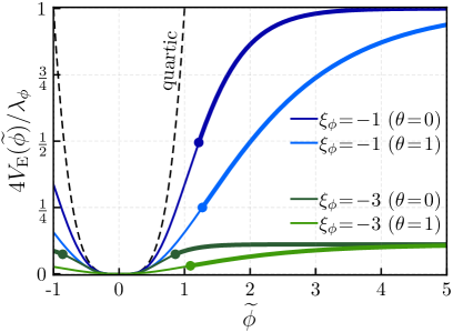
Figure 1: The inflaton potential for different curvature couplings $\xi_{\phi}$ and gravity formulations $\theta$, all of which are approximately quartic during preheating but vary substantially in the large-field region. The thick segment of each curve shows the inflationary regime of the potential, with each point marker indicating the end of inflation [coincident with Eq. (12)]. The quartic potential in the absence of a non-minimal gravitational coupling is shown (black-dashed curve) for reference.

In the large-field region $\phi\gg 1/\sqrt{-\xi_{\phi}}$, the inflaton potential then takes the form

$$V_{\rm E}(\widetilde{\phi})~{}=~{}\frac{\lambda_{\phi}}{4\xi_{\phi}^{2}}\left\{\begin{array}[]{lll}\displaystyle{\tanh^{4}\!\big{(}\sqrt{-\xi_{\phi}}\widetilde{\phi}\big{)}}&\text{for}&\theta=0\\[2.5pt] \displaystyle{\big{(}1-e^{-\sqrt{\frac{2}{3}}\widetilde{\phi}}\big{)}^{\!2}}&\text{for}&\theta=1\end{array}\right.\ ,$$ (8)

where $\widetilde{\phi}$ is the canonically normalized inflaton field. In this region, the theory acquires an approximate scale invariance and effectively approaches so-called “attractor models” which are phenomenologically viable Kallosh et al. (2013); Galante et al. (2015); Carrasco et al. (2015). In particular, for an inflationary epoch of $N$ $e$-folds, one finds a spectral index $n_{\text{s}}=1-2/N$ and tensor-to-scalar ratio $r=12\alpha/N^{2}$, where we have defined $\alpha\equiv\theta-1/(6\xi_{\phi})$.

A plot which illustrates the inflaton potential $V_{\rm E}(\widetilde{\phi})$ for a number of possible curvature couplings $\xi_{\phi}$ and gravity formulations $\theta$, all of which lead to massless preheating after inflation, is shown in Fig. 1. The inflationary trajectory is shown by the thick part of each curve, and inflation ends at the location of the point marker.

There are several constraints on our model parameters necessary to achieve viability. First, matching the observed amplitude of primordial curvature perturbations Akrami et al. (2020) fixes the relationship between $\lambda_{\phi}$ and $\xi_{\phi}$:

$$\lambda_{\phi}~{}=~{}4.9\times 10^{-10}\left(\frac{55}{N}\right)^{2}\alpha\xi_{\phi}^{2}\ .$$ (9)

Second, we must ensure that the electroweak vacuum remains stable throughout inflation. This requirement bounds the effective mass squared of the Higgs as

$$\left.\frac{\partial^{2}V_{\rm E}}{\partial\widetilde{h}^{2}}\right|_{\widetilde{h}=0}\!\!\simeq~{}\frac{g^{2}\phi^{2}}{1-\xi_{\phi}\phi^{2}}+\frac{\xi_{h}\lambda_{\phi}\phi^{4}}{(1-\xi_{\phi}\phi^{2})^{2}}~{}>~{}0$$ (10)

under the slow-roll approximation, where $\widetilde{h}$ is the canonically normalized Higgs field. The slow-roll-suppressed contributions to the Higgs mass neglected above can become more important toward the end of inflation, so the precise condition may be modified. In some inflation models, this causes inflation to end prematurely Renaux-Petel and Turzyński (2016); this may happen for $\xi_{\phi}\ll-1$ in the Palatini formalism, which is outside the scope of this paper. The constraint in Eq. (10) is simplified if we consider that during inflation $1\ll-\xi_{\phi}\phi^{2}$ and thus Eq. (10) reduces to $\lambda_{\phi}\xi_{h}-g^{2}\xi_{\phi}>0$. We shall assume that this constraint is satisfied to the extent that the Higgs is stabilized strongly at the origin during inflation. In other words, we assume that the Higgs mass is larger than the Hubble scale $H$ during inflation, and imposing this assumption, we obtain

$$\xi_{h}-\frac{g^{2}}{\lambda_{\phi}}\xi_{\phi}~{}\gg~{}\frac{1}{12}\ .$$ (11)

Third, we must also ensure that quantum corrections to the scalar potential from Higgs loops are controlled and do not ruin the above predictions for inflationary observables. To this end, if we require that $g^{2}\ll\sqrt{\lambda_{\phi}}$, then the Higgs-loop contribution is subdominant. Taking a value $\lambda_{\phi}=10^{-10}$ [based on Eq. (9)] gives the constraint explicitly as $g^{2}/\lambda_{\phi}\ll 10^{5}$, which is well within the parameter space that we shall consider.

Finally, the accelerated expansion of the universe ends once the energy density of the inflaton background falls below $\rho_{\phi}=3V(\phi)/2$, i.e., when the field falls below

$$\phi_{\rm end}~{}\equiv~{}\frac{4}{\sqrt{1+\sqrt{1-32\xi_{\phi}(1-6\theta\xi_{\phi})}}}\ .$$ (12)

Afterward, $\phi$ begins to oscillate about the minimum of the potential and we identify this point in time as the beginning of the preheating era; we focus our discussion throughout the rest of the paper on this epoch.

II.2 Cosmological Background After Inflation

Let us now discuss the evolution of the cosmological background after the end of inflation. Assuming the vacuum has been sufficiently stabilized, the Higgs field is negligible, and the cosmological background is determined solely by the dynamics of the inflaton and its potential $V_{\rm E}(\phi)\simeq V(\phi)$ in the region $\phi<\phi_{\rm end}$, where the notation $V(\phi)$ is introduced for the inflaton potential approximated in the small-field region.

The form of the inflaton potential in this region may still be sensitive to $\xi_{\phi}$. Notably, for $|\xi_{\phi}|\gg 1$ an interesting distinction appears between metric and Palatini gravity. For metric gravity, the potential is quartic at sufficiently small $\phi\ll 1/\smash{|\xi_{\phi}|}$ but becomes quadratic in the intermediate region $1/|\xi_{\phi}|\ll\phi\ll 1/\smash{\sqrt{|\xi_{\phi}|}}$. It follows that Higgs fluctuations are amplified by two different types of parametric resonance depending on the field region. By contrast, in Palatini gravity the potential is purely quartic and has no quadratic region Fu et al. (2017); Karam et al. (2021). Our model therefore offers an explicit example of purely massless preheating that is consistent with inflation, even for a large non-minimal coupling $\xi_{\phi}$. Furthermore, we can achieve the same effect with $\xi_{\phi}=\mathcal{O}(1)$, as the intermediate quadratic region vanishes. Given that the study of massless preheating is our main interest and that this occurs in the small-field region, we shall henceforth assume that $|\xi_{\phi}|\lesssim 1$ (with $\xi_{\phi}<0$).

After the end of inflation, the evolution of the background inflaton field is then well approximated by

$$\ddot{\phi}+3H\dot{\phi}+\lambda_{\phi}\phi^{3}~{}=~{}0\ ,$$ (13)

in which the dots correspond to time derivatives and $H\equiv\dot{a}/a$ is the Hubble parameter given in terms of the scale factor $a=a(t)$. As discussed in Sec. I, the approximate scale invariance of the system makes its field dynamics and resonance structure rather unique. These features have been studied extensively Greene et al. (1997) and here we briefly review them. The scale invariance is made transparent by writing Eq. (13) in terms of the conformal time $\eta\equiv\int^{t}dt^{\prime}/a(t^{\prime})$ and conformal inflaton field $\varphi\equiv a\phi$:

$$\varphi^{\prime\prime}+\lambda_{\phi}\varphi^{3}~{}=~{}0\ ,$$ (14)

where the prime notation corresponds to $\eta$ derivatives. Note that we have ignored a term proportional to $\phi^{2}R$, as this term negligibly impacts the inflaton evolution.

The approximate scale invariance of the theory is manifested by the fact that the inflaton equation of motion in Eq. (14) is independent of the cosmological expansion. The solutions carry a constant amplitude $\overline{\varphi}$ of oscillations and are given in terms of a Jacobi elliptic function

$$\varphi(x)~{}=~{}\overline{\varphi}\operatorname{cn}\left(x-x_{0},\frac{1}{\sqrt{2}}\right),$$ (16)

in which $x\equiv\smash{\sqrt{\lambda_{\phi}}}\overline{\varphi}\eta$ is the conformal time measured in units of the effective inflaton mass $\sqrt{\lambda_{\phi}}\overline{\varphi}$. The constant $x_{0}$ is used to match to the inflaton configuration at the end of inflation, and the period of oscillations in $x$ is

$$T~{}\equiv~{}4K\left(\frac{1}{\sqrt{2}}\right)~{}\approx~{}7.42\ ,$$ (17)

with $\smash{K(X)\equiv\int_{0}^{\pi/2}\!d\theta(1-X^{2}\sin^{2}\!\theta)^{-1/2}}$ defined as the complete elliptic integral of the first kind.

A cosmological energy density which is dominated by the coherent oscillations of a scalar field may behave in a variety of ways depending on the scalar potential. For example, the class of potentials $V(\phi)\propto\phi^{2n}$ (for integer $n>0$) yield a cosmological background that behaves as a fluid with the equation-of-state parameter Turner (1983)

$$w~{}\equiv~{}\frac{P}{\rho}~{}=~{}\frac{n-1}{n+1}\ ,$$ (18)

in which $P$ is the pressure and $\rho$ is the energy density, averaged over several oscillations. For the quadratic ($n=1$) and quartic ($n=2$) potentials this demonstrates the well-known result that scalar-field oscillations in these potentials correspond to perfect fluids with matter-like ($w=0$) and radiation-like ($w=1/3$) equations of state, respectively. This behavior reflects our observation in Eq. (14) that $\varphi$ evolves independently of the cosmological expansion. Namely, since the inflaton energy density scales like radiation $\rho_{\phi}\propto 1/a^{4}$, the amplitude of inflaton oscillations scale as $\overline{\phi}\propto 1/a$. Therefore, the corresponding conformal amplitude $\overline{\varphi}$ is fixed.

It also follows that in a radiation-like background the scale factor is proportional to $x$ and grows according to

$$a(x)~{}=~{}\frac{\overline{\varphi}\,x}{\sqrt{12}}\ .$$ (19)

Inflation ends once the kinetic energy grows sufficiently to have $3V(\phi)/2\leq\rho_{\phi}$, which corresponds to the time $x_{\rm end}\equiv\sqrt{12}/\phi_{\rm end}$. Note that chronologically one always has $x_{0}<x_{\rm end}$ and these are related explicitly by

$$x_{\rm end}-x_{0}~{}=~{}\text{arccn}\!\left(\!\left(\frac{2}{3}\right)^{\!\!\frac{1}{4}}\!\!,\frac{1}{2}\right)~{}\approx~{}0.45\ ;$$ (20)

for simplicity we have used $\xi_{\phi}=0$ in this expression.

Finally, in addition to the inflaton background, it is important that we examine the scalar curvature after inflation. In general, the curvature is a frame-dependent quantity with $\Omega R_{\text{J}}=4V_{\rm J}(\phi)-\dot{\phi}^{2}$ in the Jordan frame. Nevertheless, at sufficiently small $\phi$ we have $\Omega\approx 1$ and

$$a^{4}R~{} =~{}\lambda_{\phi}\varphi^{4}-\varphi^{\prime 2}$$

$$=~{}\frac{\lambda_{\phi}}{2}\overline{\varphi}{}^{4}\left[3\left(\frac{\varphi}{\overline{\varphi}}\right)^{\!\!4}-1\right]\ ,$$ (21)

where we have employed the solution in Eq. (16). The scalar curvature thus oscillates about zero and over several oscillations averages to $\langle R\rangle=3H(1-3w)=0$. However, as we shall find upon examining particle production, neither the curvature terms nor their time dependence can be neglected, as they can impart a significant contribution to the preheating dynamics.

III Production of Higgs Particles

Having established the evolution of the classical inflaton field in Sec. II.2, we can now discuss Higgs particle production in this background. We write the quantized Higgs field $\widehat{h}$ in the Heisenberg picture as a function of the fluctuations $h_{k}(t)$ of comoving momenta $k$:

$$\widehat{h}(\bm{x},t)=\!\int\!\frac{d^{3}k}{(2\pi)^{\frac{3}{2}}}\!\Big{[}\widehat{a}_{k}h_{k}(t)e^{+i\mathbf{k}\cdot\mathbf{x}}+\widehat{a}_{k}^{\dagger}h_{k}^{\!*}(t)e^{-i\mathbf{k}\cdot\mathbf{x}}\Big{]}\ ,$$ (22)

where $\widehat{a}^{\dagger}_{k}$ and $\widehat{a}_{k}$ are creation and annihilation operators, respectively. For a given comoving momentum, these fluctuations follow equations of motion

$$\ddot{h}_{k}+(3H+\Gamma_{h_{k}})\dot{h}_{k}+\omega^{2}_{h_{k}}h_{k}~{}=~{}0$$ (23)

where $\Gamma_{h_{k}}$ is a phenomenological term accounting for perturbative decays of the Higgs Kofman et al. (1997); Garcia-Bellido et al. (2009); Repond and Rubio (2016) and $\omega_{h_{k}}$ is the energy of the mode. These modes are coupled to both the oscillating inflaton background and the scalar curvature $R$, and therefore their effective masses carry an implicit time dependence. In the Jordan frame,

$$\omega_{h_{k}}^{2}~{}=~{}\frac{k^{2}}{a^{2}}+g^{2}\phi^{2}+\xi_{h}R\ .$$ (24)

However, in the Einstein frame, $\xi_{\phi}\neq 0$ generates a kinetic mixing between the inflaton field and the Higgs modes, thereby producing an inflaton-dependent friction term. We can absorb this friction into the effective mass term by the field redefinition $\mathcal{H}_{k}\equiv a\Omega^{-1/2}|_{h=0}h_{k}$ Rusak (2020), yielding the equations of motion

$$\mathcal{H}^{\prime\prime}_{k}+a\Gamma_{h_{k}}\mathcal{H}^{\prime}_{k}+\omega^{2}_{\mathcal{H}_{k}}\mathcal{H}_{k}=0,$$ (25)

in which the transformed modes are given by

$$\omega^{2}_{\mathcal{H}_{k}}=~{}k^{2}+g^{2}\varphi^{2}\!\left(\!1+\xi_{\phi}\frac{\varphi^{2}}{a^{2}}\right)+\xi a^{2}R-a^{2}\Gamma_{h_{k}}H$$ (26)

and we have defined the effective non-minimal coupling

$$\xi~{}\equiv~{}\xi_{h}+\xi_{\phi}-6\theta\xi_{h}\xi_{\phi}-\frac{1}{6}\ .$$ (27)

Note that we have neglected terms which are higher order in $a^{-1}$, such that the scalar curvature is given by $a^{4}R=\lambda_{\phi}\varphi^{4}-(\varphi^{\prime})^{2}$. In this way, we have absorbed most $\xi_{\phi}$ effects and dependence on the gravity formulation into the single effective parameter $\xi$. Finally, we confirm that if we take $\xi_{\phi}=0$, the scale invariance is restored for the conformal value $\xi_{h}=1/6$, as one would expect.

Solving the equations of motion in Eq. (25), we can track the production of Higgs particles. In particular, the comoving phase-space density of particles associated with a mode of comoving momentum $k$ is given by

$$n_{h_{k}}~{}=~{}\frac{\omega_{\mathcal{H}_{k}}}{2}\left(\frac{\left|\mathcal{H}^{\prime}\right|^{2}}{\omega_{\mathcal{H}_{k}}^{2}}+\left|\mathcal{H}_{k}\right|^{2}\right)-\frac{1}{2}\ .$$ (28)

The physical mechanism that drives this production differs considerably between the $\xi a^{2}R$ and $g^{2}\varphi^{2}$ terms. For the former, when the inflaton field passes through the minimum of its potential, one may find that a range of Higgs modes become tachyonic $\omega_{\mathcal{H}_{k}}^{2}<0$. The tachyonic instability is strongest for the smaller-momentum modes, and these modes produce particles for longer durations. By contrast, oscillations in $\varphi$ drive particle production from the latter. The resulting time-dependent modulations of $\omega_{\mathcal{H}_{k}}$ give rise to parametric resonances for Higgs modes within certain momentum bands.

Another crucial distinction between these mechanisms is found by evaluating their overall scaling under the cosmological expansion. The main term in Eq. (26) responsible for tachyonic production redshifts as $\xi a^{2}R\propto 1/a^{2}$, while the term responsible for the parametric resonance $g^{2}\varphi^{2}$ does not dissipate at all. Tachyonic production therefore always terminates after some finite time, even for the zero-momentum mode. On the other hand, production from the parametric instability continues unimpeded and ceases only once the evolution is disrupted by backreaction effects, as we cover in Sec. IV. Indeed, this distinction is ultimately traced to the Higgs-curvature interaction breaking the scale invariance that is preserved by all of the other relevant terms.

We first break our analysis into two limiting cases: one in which the quartic inflaton-Higgs interaction is dominant and the other in which the curvature interaction is dominant. Then, we explore the interplay between these interactions and finally begin to analyze the impact of perturbative Higgs decays on the field dynamics.

III.1 Production from Parametric Instability

Let us first consider the case that the curvature coupling $\xi$ is negligible and thus ignore the tachyonic production. Then, Higgs particles are produced purely from the parametric resonance associated with the $g^{2}\varphi^{2}$ term in Eq. (26). The dominant production in this case arises from the fact that as the inflaton passes through the origin, the effective masses may evolve non-adiabatically:

$$\frac{|\dot{\omega}_{\mathcal{H}_{k}}|}{\omega_{\mathcal{H}_{k}}^{2}}~{}\gtrsim~{}1\ ,$$ (29)

which triggers a burst of particle production.

The growth of the number density for a given mode is exponential and follows $\log n_{k}\simeq 2\mu_{k}x$ over several oscillations, where $\mu_{k}$ is the characteristic exponent. Note the distinction between this regular exponential growth and the stochastic growth one finds for theories without an approximate scale invariance, e.g., those with a quadratic inflaton potential Kofman et al. (1997); Greene et al. (1997). The stochastic nature of the resonance appears in these scenarios because the accumulated phase of each mode evolves with the cosmic expansion, destroying the phase coherence. In the scale-invariant theory, no such time dependence may arise and phase coherence is maintained among the modes. A more in-depth comparison of the quadratic and quartic theories, with an emphasis on the results of this paper, is provided in Appendix A.

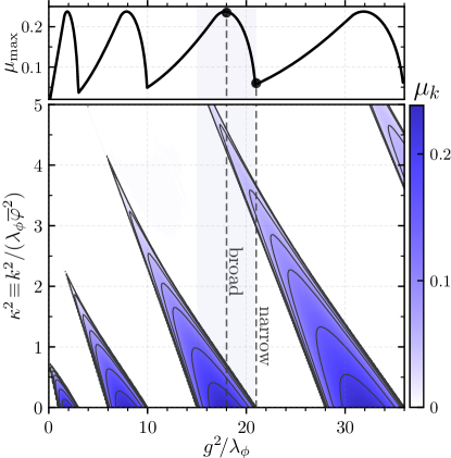
Figure 2: The instability bands of the parametric resonance arising from the inflaton-Higgs interaction (bottom panel) and the corresponding maximum characteristic exponents $\mu_{\rm max}\equiv\max_{k}\mu_{k}$ for each coupling (top panel). The contours in the bottom panel show the value of the exponent $\mu_{k}$ such that a given occupation number grows as $n_{h_{k}}\propto e^{2\mu_{k}x}$. The couplings which lead to the strongest growth are found at the center of bands which have an unstable zero mode, i.e., for $g^{2}/\lambda_{\phi}=2,8,\ldots,2n^{2}$ for $n\in\mathbb{N}$, while the weakest are found at the edge of these bands $g^{2}/\lambda_{\phi}=3,10,\ldots,2n^{2}+n$—we refer to these as the “broad” and “narrow” regimes, respectively. There is a universal $\mu_{\rm max}\approx 0.24$ for the former, while for the latter $\mu_{\rm max}$ is a non-trivial function of $g^{2}/\lambda_{\phi}$, given in Eq. (30) and plotted over an extended range in Fig. 3.

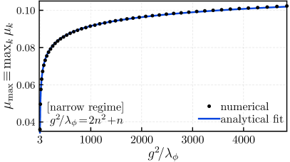
Figure 3: The maximum exponents $\mu_{\rm max}\equiv\max_{k}\mu_{k}$ for the narrow-resonance couplings $g^{2}/\lambda_{\phi}=2n^{2}+n$ (for $n\in\mathbb{N}$). These are computed numerically (point markers) and compared to the analytical fitting formula in Eq. (30) (solid curve). Note that the analytical function is evaluated only at the same discrete values $g^{2}/\lambda_{\phi}=2n^{2}+n$ in this figure, i.e., the minima of the top panel of Fig. 2. In the $g^{2}/\lambda_{\phi}\rightarrow\infty$ limit the broad/narrow regimes become degenerate with $\mu_{\rm max}\approx 0.24$, but this asymptote is approached slowly.

The size of a particular growth exponent $\mu_{k}$ is determined by a combination of the comoving momentum $k$ and the quotient $g^{2}/\lambda_{\phi}$. In Fig. 2, we have numerically solved the mode equations and plotted contours of $\mu_{k}$ in the space of these two quantities, rescaling the momentum as $\kappa\equiv k/(\sqrt{\lambda_{\phi}}\overline{\varphi})$. It is natural to separate the resonances into two different classes. The couplings with instability bands that include the zero-momentum mode, i.e., those between $2n^{2}-n<g^{2}/\lambda_{\phi}<2n^{2}+n$, for $n\in\mathbb{N}$, contain the broadest resonances and generally give the most copious particle production—we refer to these collectively as the “broad regime.” Meanwhile, those couplings with only finite-momentum bands contain the most narrow resonances and give generally weaker production, and we refer to these as the “narrow regime.” The most weak and narrow bands occur at the boundaries $g^{2}/\lambda_{\phi}=2n^{2}+n$. The distinctions between these two coupling regimes have important dynamical implications and play a major role in this paper.

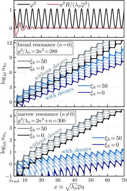
Figure 4: The evolution of background quantities $\varphi$, $a^{2}\!R$ (top panel) and Higgs phase-space density $n_{h_{k}}$ (center/bottom panels) during the early stage of preheating. The latter two panels show the broad/narrow regimes: taking $n=12$, the center panel uses a coupling $g^{2}/\lambda_{\phi}=2n^{2}$ and has a broad range of resonant modes, while the bottom panel uses the adjacent $g^{2}/\lambda_{\phi}=2n^{2}+n$ and has only a narrow range of resonant modes; the mode with the largest growth exponent is shown in each case. Additionally, these two panels show the effect of allowing for perturbative Higgs decays (first discussed in Sec. III.4, shown in blue) and non-minimal gravitational couplings $\xi_{h}$, evenly spaced over the range $0\leq\xi_{h}\leq 50$.

Although, in principle, each mode with $\mu_{k}>0$ contributes to particle production, in practice the maximum exponent of the band $\mu_{\rm max}\equiv\max_{k}\mu_{k}$ dominates. In the broad regime, the maximum exponent is $\mu_{\rm max}\approx 0.24$, found at the central values $g^{2}/\lambda_{\phi}=2n^{2}$, and this value is universal over the entire range of couplings. Conversely, the $\mu_{\rm max}$ values in the narrow regime are not universal. These features are most easily observed in the top panel of Fig. 2, where $\mu_{\rm max}$ is seen to oscillate back and forth between the broad and narrow regimes. Indeed, the growth rate of particle production is highly non-monotonic as one dials the inflaton-Higgs coupling. In fact, the narrow resonances grow to join the broad resonance at $\mu_{\rm max}\approx 0.24$ in the formal limit $g^{2}/\lambda_{\phi}\rightarrow\infty$. The non-monotonicity of $\mu_{\rm max}$ thus diminishes as a function of $g^{2}/\lambda_{\phi}$, albeit at an extremely slow pace. In what follows it proves useful to quantify this observation, so we have numerically computed $\mu_{\rm max}$ for the discrete minima of $\mu_{\rm max}$ in the narrow regime $g^{2}/\lambda_{\phi}=2n^{2}+n$ and found that they are well approximated by the function

$${\frac{\mu_{\rm max}}{0.24}~{}\approx~{}\frac{\log(Ag^{2}/\lambda_{\phi})}{1+\log(Bg^{2}/\lambda_{\phi})}}\ .$$ (30)

The constants $A=2.82$ and $B=3.34\times 10^{5}$ reproduce the numerical results to better than $1\%$ accuracy over the range $3\lesssim g^{2}/\lambda_{\phi}\lesssim 10^{4}$, which spans the full range of narrow resonances relevant to this paper. We display the function in Eq. (30) and the numerical results together in Fig. 3 for comparison. Note that the weakest resonances globally are found in the limit $g^{2}/\lambda_{\phi}\rightarrow 0$, where the bands become increasingly narrow and follow $\mu_{\rm max}\approx 0.15g^{2}/\lambda_{\phi}$ Greene et al. (1997); we shall discuss this small-coupling limit further in Sec. III.3.3.

We have plotted numerical solutions of the phase-space density $n_{h_{k}}$ in the broad and narrow regimes, for adjacent coupling bands, shown by the black curve in the top and bottom panels of Fig. 4, respectively. The mode corresponding to the most rapid growth is shown in both cases: for the broad regime this is the $\kappa=0$ mode, but for the narrow regime $\mu_{\rm max}$ corresponds to a finite momentum. We neglect the blue curves for the moment, as these first enter our discussion in Sec. III.4.

For our purposes, the non-monotonic nature of $\mu_{\rm max}$ as a function of $g^{2}/\lambda_{\phi}$ has extensive implications. In contrast to many other preheating scenarios, the magnitude of our coupling has no bearing on the growth rate of a given fluctuation—only the associated band within the repeating resonance structure is important. That said, since the width of the momentum bands increases with $g^{2}/\lambda_{\phi}$, the total number density $n_{h}$ does, in fact, depend on this coupling. We obtain the total comoving number density of the produced Higgs particles by using the saddlepoint approximation to integrate over each band:

$$n_{h}~{}\simeq~{}\frac{1}{2}\left(\!\frac{\sqrt{\lambda_{\phi}}\overline{\varphi}}{2\pi}\!\right)^{\!\!3}\left(\frac{g^{2}}{2\lambda_{\phi}}\right)^{\!\!3/4}\!\frac{e^{2\mu_{\rm max}x}}{\sqrt{\mu_{\rm max}x}}\ .$$ (31)

As this density partly determines the variance of the Higgs fluctuations, it plays a major role in assessing the metastability of the electroweak vacuum. Accordingly, we shall continue to calculate $n_{h}$ in all of the regimes.

III.2 Production from Tachyonic Instability

Let us now consider the opposite coupling limit $g\rightarrow 0$, i.e., the limit in which particle production is driven not by parametric resonance but by a tachyonic instability. The effective masses $\omega_{\mathcal{H}_{k}}$ are given by

$$\frac{\omega_{\mathcal{H}_{k}}^{2}}{\lambda_{\phi}\overline{\varphi}{}^{2}}~{}=~{}\kappa^{2}+r_{h}\left[3\left(\frac{\varphi}{\overline{\varphi}}\right)^{\!\!4}-1\right]\ ,$$ (32)

where we have defined a quantity $r_{h}\equiv\xi\overline{\varphi}{}^{2}/(2a^{2})$ that indicates the strength of the curvature term at a given time and utilized Eq. (21). We recall from Sec. II.1 that vacuum stability during inflation requires $\lambda_{\phi}\xi_{h}>\xi_{\phi}g^{2}$, and, therefore, we consider only $\xi_{h}>0$ for the moment. Indeed, for sufficiently small momenta, one finds modes that cross the tachyonic threshold $\omega_{\mathcal{H}_{k}}^{2}<0$ when the inflaton is near the minimum of its potential, triggering an exponential growth in the corresponding Higgs fluctuations. Although this growth is typically short-lived due to the redshifting of the curvature term $a^{2}\xi R\propto 1/a^{2}$, these may still be a source of copious particle production soon after inflation and thus serve as a legitimate threat to destabilize the electroweak vacuum.

There have been a number of studies devoted to calculating the rate of tachyonic particle production in different settings Felder et al. (2001b); Dufaux et al. (2006), and we employ several of those techniques in this section. Similar to Sec. III.1, near the turning points $\omega_{\mathcal{H}_{k}}^{2}=0$ the masses may change non-adiabatically and one must then compute the Bogoliubov coefficients to proceed. However, unlike in the previous section, the $\omega_{\mathcal{H}_{k}}^{2}$ may experience two distinct adiabatic segments of evolution. As long as $r_{h}\gtrsim 1$, the effective masses change adiabatically away from the turning points in both the tachyonic and non-tachyonic segments. Under this assumption, we can apply the WKB approximation by calculating the phase accumulated by modes both during the tachyonic $X_{k}\equiv\int dt\,\Omega_{h_{k}}$ (for $\smash{\Omega^{2}_{k}\equiv-\omega_{h_{k}}^{2}>0}$) and non-tachyonic $\Theta_{k}\equiv\int dt\,\omega_{h_{k}}$ segments of evolution.

Applying these methods, one finds that after passing through a tachyonic region $j$ times, the phase-space density for a given mode is written generally as Dufaux et al. (2006)

$$n_{h_{k}}~{}=~{}e^{2jX_{k}}\left(2\cos\Theta_{k}\right)^{2(j-1)}\ .$$ (33)

Hence, employing Eq. (32) we can compute the accumulated quantities $X_{k}$ and $\Theta_{k}$ for $g=0$. The details of this calculation appear in Appendix B and give

$$X_{k}~{} \simeq~{}\frac{\sqrt{2\pi}\,\Gamma(\frac{5}{4})(r_{h}-\kappa^{2})^{3/4}}{\Gamma(\frac{7}{4})(3r_{h})^{1/4}}$$

$$\Theta_{k}~{} \simeq~{}\frac{4\pi^{3/2}\sqrt{2r_{h}+\kappa^{2}}}{\Gamma(\frac{1}{4})^{2}}\ .$$ (34)

After successive bursts of tachyonic production, the growth exponent in Eq. (33) accumulates a value $\sum_{j}2jX_{k}\simeq 4\int dxX_{k}/T$, with the zero mode receiving the greatest share of the number density. The accumulated phases $\Theta_{k}$ supply only oscillatory behavior or modify the distribution over momenta. Given that our primary concern is the overall growth of the Higgs number density, we shall neglect these quantities. Then, we can estimate that

$$n_{h_{k}}~{}\simeq~{}\left(\frac{x}{x_{0}}\right)^{\!\!4\sqrt{\!\frac{2\xi}{3\sqrt{3}}}}\!\exp\left[-\frac{2(x^{2}-x_{0}^{2})\kappa^{2}}{3^{9/4}\sqrt{\xi}}\right]\ ,$$ (35)

which holds for the duration of the tachyonic instability.

Let us focus on the $\kappa=0$ mode, which experiences the strongest growth in the tachyonic regime. At first glance, the growth may actually appear weak in comparison to the parametric resonance [in Eq. (31)] since it is not exponential in time—it merely obeys a power law. The difference is that the power scales with $\sqrt{\xi}$ and has no upper bound, in line with studies of the tachyonic instability in other settings Dufaux et al. (2006); Ema et al. (2016). This feature sharply contrasts with the parametric resonance, in which the $\mu_{\rm max}$ growth rate is bounded universally from above (as we observed in Fig. 2), regardless of the coupling.

Of course, as the universe expands the tachyonic production soon terminates. In particular, as $r_{h}$ redshifts to values below unity, the tachyonic masses $\Omega_{h_{k}}$ are suppressed and the adiabatic assumption breaks down. Using $|\dot{\Omega}_{h_{k}}|\gtrsim\Omega_{h_{k}}^{2}$ as the threshold for where this breakdown occurs, we find $r_{h}^{2}\gtrsim(r_{h}-\kappa^{2})^{3}$. This condition implies that the span of modes exposed to the instability is bounded above by $\kappa\lesssim\sqrt{r_{h}}$ and that a given mode is active for $x\lesssim\sqrt{6\xi}/\!\max(1,\kappa)$. The modes shut down successively, starting with the largest-momentum modes, such that tachyonic production ends at the time

$$x_{\xi}~{}\simeq~{}\sqrt{6\xi}\ .$$ (36)

The total number density of Higgs particles is given by integrating Eq. (35) over the phase space, but a cutoff $\kappa\lesssim r_{h}^{2}$ should be imposed on each momentum band per the discussion above. We again use the saddlepoint approximation to perform the integration and obtain a comoving number density

$$n_{h}~{}\simeq~{}\frac{1}{8}\Big{(}\sqrt{\lambda_{\phi}}\overline{\varphi}\Big{)}^{3}\left(\frac{3^{9/4}\!\sqrt{\xi}}{2\pi x^{2}}\right)^{\!\!3/2}\!\!\left(\frac{x}{x_{0}}\right)^{\!\!4\sqrt{\frac{2\xi}{3\sqrt{3}}}}\ ,$$ (37)

which is applicable for $x\lesssim x_{\xi}$. Although there is a brief transient phase of non-adiabatic production for $x\gtrsim x_{\xi}$, particle production from the curvature term proceeds only through the substantially weaker narrow resonance, which shuts down entirely soon thereafter. We cover the details of this regime in Sec. III.3.3 below.

III.3 Production in the Mixed Case

Let us now promote our discussion to the mixed case, in which both couplings $g^{2}/\lambda_{\phi}$ and $\xi$ are non-zero. As such, the Higgs modes evolve with the effective masses

$$\frac{\omega_{\mathcal{H}_{k}}^{2}}{\lambda_{\phi}\overline{\varphi}{}^{2}}=\kappa^{2}+\frac{g^{2}}{\lambda_{\phi}}\left(\frac{\varphi}{\overline{\varphi}}\right)^{\!\!2}\!\left[1\!-\!2r_{\phi}\!\left(\frac{\varphi}{\overline{\varphi}}\right)^{\!\!2}\right]\!+r_{h}\!\left[3\left(\frac{\varphi}{\overline{\varphi}}\right)^{\!\!4}\!-\!1\right]$$ (38)

that follow directly from Eq. (26), and by analogy to $r_{h}$ we have defined $r_{\phi}\equiv-\xi_{\phi}\overline{\varphi}{}^{2}/(2a^{2})$.

There are several immediate implications; let us discuss these with a focus on the effect of the Higgs-curvature coupling. First, since only the curvature term dissipates with the cosmological expansion, the dynamics may progress through several distinct phases, most noticeably if $r_{h}\gg g^{2}/\lambda_{\phi}$ at early times. Second, the reintroduction of the $g^{2}\varphi^{2}$ term lifts the effective masses and thereby opens the $\xi<0$ region to viability. Indeed, the $\xi<0$ region was excluded in Sec. III.2 only because the inflationary constraints [in Eq. (10) and Eq. (11)] would have been violated, but for mixed couplings this half of parameter space can be reincorporated. Third, the small-coupling regime ($g^{2}/\lambda_{\phi}\lesssim 1$ and $r_{h}\lesssim 1$) stands apart from most of our discussion thus far. The particle production in this regime is driven entirely by narrow parametric resonances arising from two different types of modulations $(\varphi/\overline{\varphi})^{2}$ and $(\varphi/\overline{\varphi})^{4}$. If these modulations can be approximated as sinusoidal, then a perturbative treatment is likely effective. We investigate all of these possible scenarios below.

III.3.1 Dominant $g^{2}\phi^{2}$ (with $g^{2}/\lambda_{\phi}\gg 1$)

The simplest possibility is an initially small curvature term $|r_{h}|\lesssim g^{2}/\lambda_{\phi}$, since this does not allow a tachyonic instability to develop during preheating. (We confine our discussion to $g^{2}/\lambda_{\phi}\gg 1$ for the moment and cover the small-coupling regime separately.)

Nonetheless, the curvature term in this case has an impact on the Higgs dynamics. Depending on the sign of $\xi$, these terms may add constructively or destructively, enhancing or suppressing the effective masses $\omega_{\mathcal{H}_{k}}$, respectively. For $\xi>0$, the effect is constructive and the resonance bands are widened; e.g., the broad instability bands are extended to $\kappa^{2}\leq\sqrt{2g^{2}/(\pi^{2}\lambda_{\phi})+r_{h}}$. We have seen that Fig. 4 falls within this category, and this extension explains the variation among different $\xi$. Conversely, for $\xi<0$ the effect is destructive: not only do the bands narrow, but the non-adiabaticity that drives the parametric resonance is weakened. Explicitly, the maximum characteristic exponent is reduced to

$$\max_{g^{2}/\lambda_{\phi}}\mu_{\rm max}~{}=~{}\frac{2}{T}\log\!\left(\!e^{-\frac{\pi r_{h}^{2}}{g^{2}/\lambda_{\phi}}}\!+\sqrt{1+e^{-\frac{2\pi r_{h}^{2}}{g^{2}/\lambda_{\phi}}}}\hskip 1.99168pt\right)\ .$$ (39)

Surely, after a sufficient duration one has $r_{h}\lesssim\sqrt{g^{2}/\lambda_{\phi}}$ and the exponent $\mu_{\rm max}\approx 0.24$ is restored. In other words, the full capacity of the parametric resonance is delayed until a time $x_{g}$, which is given approximately by

$$x_{g}~{}\simeq~{}\sqrt{-6\xi}\left(2\pi\frac{\lambda_{\phi}}{g^{2}}\right)^{\!\!1/4}\ .$$ (40)

After this time the curvature term continues to dissipate and has an increasingly negligible influence. The growth of fluctuations then proceeds according to Sec. III.1.

III.3.2 Dominant $\xi Rh^{2}$ (with $g^{2}/\lambda_{\phi}\gg 1$)

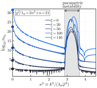
Figure 5: The phase-space density of Higgs particles $n_{h_{k}}$ produced during preheating, computed numerically and evaluated at the time $x=400$. The point markers along the vertical axis show our analytical result for $n_{h_{0}}$, found by evaluating Eq. (42) at zero momentum. The Higgs-inflaton coupling chosen $g^{2}/\lambda_{\phi}=21$ corresponds to a narrow resonance, and the different curves show various choices for the curvature coupling $\xi$. The only production from the quartic interaction occurs at finite momenta (gray region) and the curvature interaction dominates the production at small momenta.

An initially large $r_{h}\gg g^{2}/\lambda_{\phi}\gg 1$ ensures the Higgs dynamics are dominated by tachyonic production until a time $x_{\xi}$. Unlike the converse situation above, where we could ignore the curvature interaction after some duration, there is no regime in which we can ignore the $g^{2}\phi^{2}$ interaction entirely. Aside from the fact that the parametric resonance from this term will always play a role, its presence also alters the size of the tachyonic masses. We can incorporate this effect by performing an analysis along the lines of Sec. III.2 with $g^{2}/\lambda_{\phi}\neq 0$. Then, for a given mode, we find that when $\sqrt{g^{2}/\lambda_{\phi}}\lesssim r_{h}\lesssim g^{2}/\lambda_{\phi}+\kappa^{2}$ is satisfied the tachyonic instability is active and proceeds adiabatically. In order to compute the integral analytically, we assume that $(g^{2}/\lambda_{\phi})^{2}\gg(r_{h}-\kappa^{2})(3r_{h}-2r_{\phi}g^{2}/\lambda_{\phi})$. Then, the accumulated quantities [from Eq. (33)] are found to be

$$X_{k}\simeq\frac{\pi(r_{h}-\kappa^{2})}{\sqrt{2g^{2}/\lambda_{\phi}}}\ ,\quad\ \Theta_{k}\simeq\frac{\pi\sqrt{g^{2}/\lambda_{\phi}-r_{h}+\kappa^{2}}}{\sqrt{2}}\ .$$ (41)

As expected, Eq. (41) shows that tachyonic production is still concentrated in the small-momentum modes. However, the evolution of $n_{h_{k}}$ in the presence of $g^{2}/\lambda_{\phi}\neq 0$ is markedly different. Rather than a power law, the phase-space density rapidly asymptotes to a constant as

$$\log n_{h_{k}}~{}\simeq~{}\frac{12\sqrt{2}\pi\xi}{T\sqrt{g^{2}/\lambda_{\phi}}}\left[\frac{1}{x_{0}}-\frac{1}{x}-\frac{(x-x_{0})\kappa^{2}}{6\xi}\right]\ ,$$ (42)

again neglecting the oscillatory component $\cos\Theta_{k}$. The termination of the tachyonic resonance is pushed to an earlier time depending on the quartic couplings:

$$x_{\xi}~{}\simeq~{}\sqrt{\!\frac{6\xi}{\sqrt{g^{2}/\lambda_{\phi}}}}\ .$$ (43)

Afterward, the modes grow as $n_{h_{k}}\propto e^{2\mu_{k}x}$, driven by the parametric resonance. The phase-space density can be found at these times by matching to Eq. (42) at $x_{\xi}$.

Finally, the number density of Higgs particles produced during this tachyonic phase is found by integrating Eq. (42). Using the saddlepoint approximation we find

$$n_{h}~{}\simeq~{}\frac{(\!\sqrt{\lambda_{\phi}}\overline{\varphi})^{3}}{8\pi^{3}}\!\left(\!\frac{T}{2x}\sqrt{\frac{g^{2}}{2\lambda_{\phi}}}\right)^{\!\!\!3/2}\!\!\!e^{\frac{12\sqrt{2}\pi\xi}{T\sqrt{g^{2}/\lambda_{\phi}}}\left(\frac{1}{x_{0}}-\frac{1}{x}\right)}\ .$$ (44)

In Fig. 5 we have plotted the phase-space density $n_{h_{k}}$, calculated numerically over the momentum space of the Higgs modes. The quartic coupling chosen $g^{2}/\lambda_{\phi}=21$ sits on a narrow resonance and therefore produces particles only at finite momenta (highlighted by the gray region). Meanwhile, the different curves show various non-minimal couplings $\xi$. Because the parametric resonance yields unimpeded particle production, the finite-momentum peak in $n_{h_{k}}$ continues to grow with time, while production for the other modes ceases once $x\gtrsim x_{\xi}$. The large point markers along the vertical axis show agreement with our analytical result for $n_{h_{0}}$ where the tachyonic production is dominant, found by evaluating Eq. (42) at zero momentum.

The same logic as above may be applied to the $\xi<0$ region of parameter space. As this region is dominated by tachyonic particle production, we may again employ Eq. (33) to calculate the generated Higgs spectrum. While this calculation is straightforward in principle, it requires some additional technical details that we include in Appendix B, but we summarize the results here. The phase-space density for the Higgs is given by

$$\log n_{h_{k}}\simeq\frac{4H_{1}(3,0)}{T}\!\!\int\!dx\,\frac{\kappa^{2}\!-2r_{h}+\frac{g^{2}}{\lambda_{\phi}}\!\left(2r_{\phi}\!-\!1\right)}{\sqrt{\kappa^{2}-r_{h}}}\ ,$$ (45)

where $H_{1}(3,0)\approx 0.76$ corresponds to the function defined in Eq. (91) of Appendix B. The small-momentum modes provide the largest contribution, and we can approximate

$$\log n_{h_{0}}~{}\simeq~{} \frac{8H_{1}(3,0)}{T}\!\left(\!1+\frac{g^{2}}{\lambda_{\phi}}\frac{\xi_{\phi}}{\xi}\!\right)\!\sqrt{6|\xi|}\log\!\left(\frac{x}{x_{0}}\right)$$

$$-\frac{H_{1}(3,0)}{T}\sqrt{\frac{2}{-3\xi}}\frac{g^{2}}{\lambda_{\phi}}(x^{2}-x_{0}^{2})$$ (46)

in this limit. Compared to $\xi>0$, the power indices are a similar magnitude if we neglect the effect of $\xi_{\phi}$.

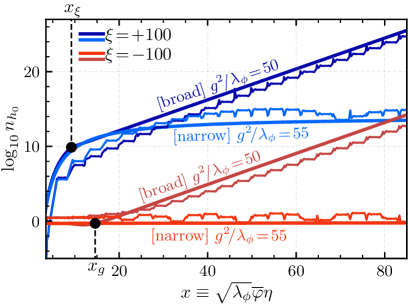
Figure 6: The growth of the zero-mode phase-space density in the mixed-coupling case, exploring both signs $\xi=\pm 100$ and the broad and narrow regimes of the parametric resonance. The thin (thick) curves show our numerical (analytical) results, respectively. For $\xi>0$, the tachyonic instability drives particle production early on [following Eq. (42)], but once $x\gtrsim x_{\xi}$ it is driven by the parametric resonance $n_{k}\propto e^{2\mu_{k}x}$. The quartic and curvature contributions add constructively and enhance the instability. Meanwhile, for $\xi<0$, these contributions add destructively, and the growth exponent $\mu_{k}$ is effectively shut off [following Eq. (39)] until the time $x_{g}$.

In Fig. 6, we demonstrate the growth of the zero-mode $n_{h_{0}}$ in the mixed-coupling case, showing both our numerical (thin curves) and analytical (thick curves) results. For comparison, we have included both the positive (blue curves) and negative (red curves) $\xi$ regimes, as well as the narrow and broad resonance regimes. The destructive effect of $\xi<0$ is evident, as changing the sign of $\xi$ induces a gap of many orders of magnitude in the zero-mode density. As a result, we should expect that electroweak vacuum metastability shows a preference for the $\xi<0$ half of parameter space. We shall return to this topic when we examine Higgs destabilization in Sec. IV.

III.3.3 Small-Coupling Regime

Let us now focus on the small-coupling regime, i.e., where both $g^{2}/\lambda_{\phi}\lesssim 1$ and $|r_{h}|\lesssim 1$. The latter inequality is always imminent, so we are free to also interpret this regime as the late-time behavior of a model with $g^{2}/\lambda_{\phi}\lesssim 1$ and an arbitrary curvature coupling. Indeed, as soon as $|r_{h}|\lesssim 1$ the tachyonic instability transitions into a narrow resonance. In fact, both of the instabilities in this regime experience a narrow parametric resonance, and our analysis should follow a different approach. Namely, the oscillatory terms in Eq. (38) act as small modulations to $\omega_{\mathcal{H}_{k}}^{2}$, and we can treat these terms perturbatively Greene et al. (1997). We expand the elliptic functions as

$$\left(\frac{\varphi}{\overline{\varphi}}\right)^{\!2}\!\!~{} =~{}\sum_{\ell=0}^{\infty}F_{\ell}\cos\frac{4\pi\ell(x-x_{0})}{T}$$

$$\left(\frac{\varphi}{\overline{\varphi}}\right)^{\!4}\!\!~{} =~{}\sum_{\ell=0}^{\infty}G_{\ell}\cos\frac{4\pi\ell(x-x_{0})}{T}\ ,$$ (47)

with the leading five coefficients given in Table 1. Noting that the series converges quickly after the first three terms, we truncate at order $\ell=2$ and the expansion serves as a good approximation. Moreover, given that $r_{h}$ are slowly varying compared to the timescale of inflaton oscillations, the Higgs mode equations take the form of the Whittaker-Hill equation:

$$\frac{d^{2}\mathcal{H}_{k}}{dz^{2}}+\left(A_{k}+2p\cos 2z+2q\cos 4z\right)\mathcal{H}_{k}~{}=~{}0\ ,$$ (48)

where we have defined $z\equiv 2\pi(x-x_{0})/T$. The coefficients of the frequency terms are given by

$$A_{k}=\left(\frac{T}{2\pi}\right)^{\!2}\!\Big{[}\kappa^{2}+\frac{g^{2}}{\lambda_{\phi}}(F_{0}-2r_{\phi}G_{0})+r_{h}(3G_{0}-1)\Big{]}$$ (49)

in which we have defined the quantities

$$p~{} =~{}-\frac{1}{2}\left(\frac{T}{2\pi}\right)^{\!2}\left[\frac{g^{2}}{\lambda_{\phi}}(F_{1}-2r_{\phi}G_{1})+3r_{h}G_{1}\right]$$

$$q~{} =~{}+\frac{1}{2}\left(\frac{T}{2\pi}\right)^{\!2}\left[\frac{g^{2}}{\lambda_{\phi}}(F_{2}-2r_{\phi}G_{2})+3r_{h}G_{2}\right]\ .$$ (50)

Using Floquet theory it is relatively straightforward to calculate the characteristic exponents $\mu_{k}$ for the unstable modes Whittaker and Watson (1996); Lachapelle and Brandenberger (2009). We can therefore find the maximum exponents $\mu_{\rm max}\equiv\max_{k}\mu_{k}$ over the small-coupling parameter space. These results are displayed in Fig. 7.

Table 1: Coefficients for the expansions in Eq. (47).

$\ell$	$0$	$1$	$2$	$3$	$4$
$F_{\ell}$	$0.457$	$0.497$	$4.29\times 10^{-2}$	$2.78\times 10^{-3}$	$1.60\times 10^{-4}$
$G_{\ell}$	$0.333$	$0.476$	$0.164$	$2.39\times 10^{-2}$	$2.45\times 10^{-3}$

An interesting feature of Fig. 7 is that, given the scale-factor dependence of $r_{h}$, we can interpret the figure as showing the flow of $\mu_{\rm max}$ as a function of time. For some initial $r_{h}\neq 0$ value, $\mu_{\rm max}$ flows along contours of constant $g^{2}/\lambda_{\phi}$ (e.g., the gray arrows) until it reaches the $r_{h}=0$ axis. Notably, for $\xi<0$ the evolution of $\mu_{\rm max}$ over this time is not necessarily monotonic. For larger quartic couplings, one may enter the $\mu_{\rm max}=0$ region (enclosed by red curves) and then exit it while approaching $r_{h}=0$.

Note that in the regime of negligible curvature couplings, Eq. (48) reduces to the form of the Mathieu equation. The Mathieu equation is familiar from models of massive preheating, but unlike such models the parametric instability from the $g^{2}\phi^{2}$ interaction does not terminate due to the approximate scale invariance of the theory. The fact that the curvature contributions are neither long-lived nor tachyonic means that the quartic contribution becomes the most salient in the small-coupling regime. Even for couplings as large as $r_{h}=\mathcal{O}(g^{2}/\lambda_{\phi})$, the resonance bands are widened, but their influence only induces a logarithmic correction to the growth rates.

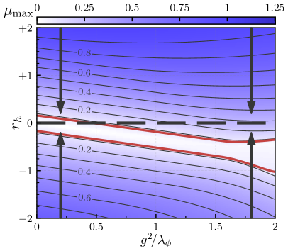
Figure 7: Contours of the maximum characteristic exponent $\mu_{\rm max}\equiv\max_{k}\mu_{k}$ shown over the space of small couplings $\{g^{2}/\lambda_{\phi},r_{h}\}$ with $\xi_{\phi}=0$ for simplicity. Because the curvature parameter redshifts as $|r_{h}|\propto 1/a^{2}$, this figure may be interpreted in a time-dependent way. From some initial point, the $\mu_{\rm max}$ value flows along lines of fixed $g^{2}/\lambda_{\phi}$ toward $|r_{h}|\rightarrow 0$ (illustrated by gray arrows) before finally landing along the narrow quartic resonance $\mu_{\rm max}\approx 0.15g^{2}/\lambda_{\phi}$ (gray-dashed line).

For these reasons, the $r_{h}\rightarrow 0$ limit is usually the most pertinent in the context of vacuum metastability. Here, the modes grow as $n_{h_{k}}\approx e^{2\mu_{k}x}/2$ for momenta around the narrow bands. The primary resonance is centered at $\kappa^{2}=2\pi/T$, and one finds the maximum exponent $\mu_{\rm max}=F_{1}Tg^{2}\!/(8\pi\lambda_{\phi})\approx 0.15g^{2}/\lambda_{\phi}$ Greene et al. (1997). Using the saddlepoint approximation, we integrate to find

$$n_{h}~{}\simeq~{}\frac{\pi\lambda_{\phi}\overline{\varphi}{}^{3}}{T^{2}}\sqrt{\frac{2\lambda_{\phi}\mu_{\rm max}}{Tx}}e^{2\mu_{\rm max}x}\ .$$ (51)

III.4 Perturbative Higgs Decays

Thus far, for simplicity we have neglected the perturbative decay of Higgs particles after their production. These decays may not appear important when considering the substantial rates of steady non-perturbative particle production. After all, perturbative decays are known to have only a minor effect in preheating with massive inflaton potentials (see Appendix A). However, given the unique properties that appear for massless preheating, it is worth examining the Higgs decays in closer detail.

Before continuing on this path, let us briefly address the other ways in which the Higgs may transfer its energy density, most notably the non-perturbative production of gauge bosons. Even though the Higgs mass term oscillates coherently due to the inflaton-field motion, the gauge-field mass terms do not oscillate uniformly. Therefore, in the early stages of preheating, we expect that resonant production of $W$ and $Z$ gauge bosons from the Higgs evolution is less significant than resonant production of the Higgs field itself. Still, the averaged value of the gauge-boson mass terms are modulated by the time dependence of $\langle h^{2}\rangle$, so a substantial amount of gauge bosons could be produced. As long as the Higgs field is much smaller than the critical value in Eq. (52), a simple analysis shows that the gauge-field production from fast oscillations of $\langle h^{2}\rangle$ is in the narrow regime. More precise estimation of gauge-field production requires a dedicated study (see also footnote 3). In the following, we shall therefore assume that non-perturbative gauge-field production induced by the Higgs field can be ignored and that perturbative decays are the dominant mechanism through which energy is transferred out of the Higgs field.

In the early stages of preheating, we expect that perturbative decay channels for the Higgs are kinematically accessible since the homogeneous background value for $h$ is negligible. Even if a background value is generated, the masses of SM particles are lighter than the Higgs during preheating as long as $h\ll h_{\rm crit}$, in which

$$h_{\rm crit}~{}=~{}\sqrt{\frac{g^{2}\phi^{2}+\xi_{h}R}{\left|\lambda_{h}\right|}}$$ (52)

is the Higgs value at the barrier separating the false and true vacua, i.e., the local maximum of the potential.

Therefore, the dominant decay channel of the Higgs is into top quarks at a rate

$$\Gamma_{h}~{}\simeq~{}\frac{3y_{t}^{2}m_{h}}{16\pi}$$ (53)

in the rest frame, where $y_{t}$ is the top Yukawa coupling, evaluated at the Higgs mass scale, and we have denoted

$$m_{h}~{}=~{}\sqrt{g^{2}\phi^{2}+\xi_{h}R}$$ (54)

as the effective Higgs mass. In general, we should include a Lorentz factor $\gamma=\omega_{h_{k}}/m_{h}$ which suppresses the decay rate for relativistic particles. The tachyonic instability produces particles with physical momenta $k/a\lesssim\overline{\phi}{}^{2}\sqrt{\xi\lambda_{\phi}/2}$, which translates to $\gamma\simeq\mathcal{O}(1)$ and does not appreciably suppress the rate. Likewise, the parametric instability with $g^{2}/\lambda_{\phi}\gg 1$ produces particles with $k/a\lesssim[\lambda_{\phi}\overline{\phi}{}^{2}\sqrt{g^{2}/\lambda_{\phi}}]^{1/2}$, which is non-relativistic. The exception is small couplings $g^{2}/\lambda_{\phi}\ll 1$, for which Higgs production is dominated by particles with a Lorentz factor $\gamma\simeq k/(am_{h})\simeq\sqrt{\lambda_{\phi}/g^{2}}$. While we include the full effect of this time-dilation on the decay rate in our numerical computations, our analytical calculations are performed assuming that $\gamma\simeq\max(1,\sqrt{\lambda_{\phi}/g^{2}})$.

Naturally, as perturbative decays exponentially suppress the number density, they work against the non-perturbative production processes above. The field dependence of the effective Higgs mass $m_{h}$ implies an interesting chronology of events. If the parametric resonance is the dominant production mechanism, then a burst of particles is produced as $\phi$ passes through the origin. Meanwhile, decays are strongest when $\phi$ is maximally displaced. The result is that rather than $n_{h_{k}}$ maintaining a constant value during its adiabatic evolution, it is exponentially suppressed at the rate $\Gamma_{h}$. However, due to its dependence on evolving background quantities, the decay rate is a non-trivial function of time. The effect on the number density is to dissipate it as

$$\log n_{h_{k}}~{}\propto~{}-\int dt\,\frac{\Gamma_{h}}{\gamma}~{}=~{}-\int dx\,\frac{a\Gamma_{h}}{\gamma\sqrt{\lambda_{\phi}}\overline{\varphi}}$$ (55)

where the integration is performed over times when decays are kinematically possible.

An important limit is that in which the non-minimal couplings $\xi_{h},\xi_{\phi}$ are negligible, as this also represents the system for times $x\gtrsim x_{\xi}$. The pivotal observation is that the effective decay rate scales as $a\Gamma_{h}\propto|\varphi|$ and thus has no overall scale-factor dependence, allowing a direct competition between the production and decay rates to determine the fate of the electroweak vacuum; this contrasts with massive preheating, in which the decay exponent carries a logarithmic time dependence. (We refer to Appendix A for a more thorough comparison.) Explicitly, the time-averaged conformal decay rate $\langle a\Gamma_{h}\rangle$ is given by

$$\frac{\left\langle a\Gamma_{h}\right\rangle}{\sqrt{\lambda_{\phi}}\overline{\varphi}}~{}=~{}\frac{3y_{t}^{2}}{16\pi}\sqrt{\frac{g^{2}}{\lambda_{\phi}}}\left\langle\frac{\left|\varphi\right|}{\overline{\varphi}}\right\rangle~{}\approx~{}0.036y_{t}^{2}\sqrt{\frac{g^{2}}{\lambda_{\phi}}}\ ,$$ (56)

where we have assumed the regime $g^{2}/\lambda_{\phi}\gtrsim 1$. Indeed, we find that the number density of Higgs particles does not grow for couplings exceeding

$$\frac{g^{2}}{\lambda_{\phi}}~{}\gtrsim~{}2.8\times 10^{3}\left(\frac{\mu_{\rm max}}{0.24}\right)^{\!2}\!\left(\frac{y_{t}}{0.5}\right)^{\!-4}\ .$$ (57)

Remarkably, this result suggests that electroweak vacuum metastability can be achieved in massless preheating. Moreover, metastability is given not by an upper bound but by a lower bound on the quartic coupling (see also Refs. Choi et al. (2019); Lebedev and Yoon (2021)).

In the opposite limit, where $g$ is negligible and the curvature term dominates, neither the production or perturbative decays evolve exponentially. In particular, we have $\left\langle a\Gamma_{h}\right\rangle\propto\log a$ and a growth rate that is dominant at early times. The result is that perturbative decays do not quell the early phase of tachyonic production, but if the vacuum survives, decays increasingly dissipate the fluctuations as the system evolves.

Looking back to Fig. 4, we have demonstrated the effect of the perturbative decays on particle production by plotting $n_{h_{k}}$ both with (blue curves) and without (grayscale curves) the decays incorporated. Clearly, in the absence of decays, the phase-space density remains constant when the inflaton is away from $\phi\approx 0$, as the $n_{h_{k}}$ correspond to an adiabatic invariant. However, when the Higgs decays are turned on, the curves show a dissipation during the adiabatic evolution. The dissipation does not always appear to be at a constant rate, reflecting that in our numerical computations, the decay rates are not averaged as in Eq. (56) but are given instantaneously as a function of the effective Higgs mass $m_{h}$.

Before concluding this section, we put aside the Higgs for a moment and make some remarks regarding the quantum fluctuations of the inflaton field. An extensive part of the discussion in this section can be applied by analogy to the production of inflaton particles. These particles are generated through the inflaton self-coupling, so that the effective masses [analogous to Eq. (24)] are

$$\omega_{\phi_{k}}^{2}~{}=~{}\frac{k^{2}}{a^{2}}+3\lambda_{\phi}\phi^{2},$$ (58)

in the Jordan frame, or also in the Einstein frame after neglecting higher-order terms in $\mathcal{O}(a^{-2})$. In fact, production via this inflaton “self-resonance” is understood by the simple replacement $g^{2}/\lambda_{\phi}=3$ in the analysis of Sec. III.1 Greene et al. (1997). For example, from our result for the Higgs number density $n_{h}$ in Eq. (31), we can estimate the inflaton number density $n_{\phi}$ with appropriate replacements. Interestingly, the characteristic growth exponent $\mu_{\rm max}\approx 0.036$ for inflaton production corresponds to the weakest of the $g^{2}/\lambda_{\phi}\geq 1$ regime. In Sec. IV below, we shall find that this self-resonance and its properties are extremely material to the discussion of vacuum destabilization and the end of preheating.

IV Backreaction and Vacuum Destabilization

While Sec. III provides the groundwork for our study of electroweak vacuum metastability, an essential ingredient is still absent from our analysis. In particular, recalling our assumption that the Higgs field has a negligible background value $h\approx 0$, the term in the potential which threatens to destabilize the vacuum (the self-interaction $\lambda_{h}h^{4}/4$) has not yet entered our analysis. In order to incorporate the unstable vacuum, we must consider not only the growth of Higgs fluctuations but also the backreaction that these fluctuations have on the system. As discussed in Sec. I, although the fluctuations in massless preheating appear to grow unimpeded, they will inevitably grow large enough to either trigger vacuum decay or disrupt the background inflaton evolution through backreaction.

A complete treatment of the backreaction and non-linearities that appear, especially in the later stages of preheating, requires numerical lattice simulations. However, we find that, in order to probe the Higgs stability, or estimate the onset of the non-linear stage, the one-loop Hartree approximation Boyanovsky et al. (1995) is sufficient. That is, we assume the factorization $h^{4}\rightarrow 6\langle h^{2}\rangle h^{2}-3\langle h^{2}\rangle^{2}$ for the quartic term in the Lagrangian (and an analogous expression for the inflaton), where the expectation values are given by

$$\langle h^{2}\rangle~{} =~{}\frac{1}{(2\pi)^{3}}\int d^{3}k\left|h_{k}\right|^{2}$$ (59)

$$\langle\phi^{2}\rangle~{} =~{}\frac{1}{(2\pi)^{3}}\int d^{3}k\left|\phi_{k}\right|^{2}\ .$$ (60)

In turn, the effective masses for the Higgs and inflaton modes—from Eq. (24) and Eq. (58), respectively—are modified as the variance of the fluctuations grows:

$$\omega_{h_{k}}^{2}~{} =~{}\frac{k^{2}}{a^{2}}+g^{2}\phi^{2}+\xi_{h}R+g^{2}\langle\phi^{2}\rangle+3\lambda_{h}\langle h^{2}\rangle$$ (61)

$$\omega_{\phi_{k}}^{2}~{} =~{}\frac{k^{2}}{a^{2}}+3\lambda_{\phi}\phi^{2}+g^{2}\langle h^{2}\rangle+3\lambda_{\phi}\langle\phi^{2}\rangle\ .$$ (62)

The fluctuations also couple to the inflaton background, modifying the equation of motion as

$$\ddot{\phi}+3H\dot{\phi}+\lambda_{\phi}\phi^{3}+\left(3\lambda_{\phi}\langle\phi^{2}\rangle+g^{2}\langle h^{2}\rangle\right)\phi~{}=~{}0\ .$$ (63)

Given that the motion of $\phi$ drives the particle-production processes, once these oscillations are disrupted the dynamics of the type discussed in Sec. III is shut down. The termination of these processes generally coincides with the energy density of the fluctuations growing comparable to that of the inflaton background and thus corresponds to the end of the linear stage of preheating.

We shall include all of the Hartree terms in our numerical calculations (as detailed in Appendix C), but the corrections from the self-interactions $3\lambda_{h}\langle h^{2}\rangle$ and $3\lambda_{\phi}\langle\phi^{2}\rangle$ will tend to carry the most weight for our analytical calculations. We find that from simple analytic estimates we can reproduce the salient lattice simulation results in the literature. For further validation, our numerical analyses are also compared to the literature on models for which the inflaton potential is quadratic in Appendix A. For further discussion on the non-linear dynamics and backreaction in preheating, we refer the reader to Refs. Kofman et al. (1997); Greene et al. (1997).

The main results of Sec. III consist of the produced number density $n_{h}$, so it is necessary to translate between these quantities and the variance $\langle h^{2}\rangle$. While one can fully express $\langle h^{2}\rangle$ in terms of Bogoliubov coefficients, the result is a sum of two terms, one of which is rapidly oscillating and not important for our purpose of producing order-of-magnitude estimates Kofman et al. (1997). As long as the produced Higgs particles are non-relativistic one can write $\langle h^{2}\rangle\simeq n_{h}/(a^{3}\omega_{h})$, with a similar expression applying to the inflaton or any other relevant fields. Note that the number density is well defined only when evolving adiabatically, so the points at which we evaluate $\omega_{h_{k}}$ must remain consistent with this assumption.

IV.1 Onset of Non-Linear Stage

In the context of vacuum metastability, a natural concern is that particle-production processes arising from scale-invariant terms do not terminate in the linear stage of preheating. That is, these processes terminate only once field fluctuations become so large that they significantly backreact on the system at some time $x_{\rm NL}$. The longer the linear stage lasts, the more concern for vacuum destabilization since the Higgs fluctuations must remain sufficiently controlled over this entire duration.

In our model, either the Higgs or inflaton fluctuations may bring about an end to the linear stage, but a spectator field could potentially play this role as well (see Sec. V for further discussion along these lines). Let us first examine the necessary conditions for the Higgs to play this role. There are two competing effects that influence the background inflaton field Greene et al. (1997). On the one hand, as the inflaton loses energy to particle production, $\overline{\varphi}$ falls and thereby decreases the effective frequency of oscillations $\sqrt{\lambda_{\phi}}\,\overline{\phi}$. On the other hand, as the Higgs variance grows the inflaton obtains an effective mass $\sqrt{g^{2}\langle h^{2}\rangle}$, increasing the oscillation frequency. The inflaton oscillations are disrupted once these two quantities are similar in magnitude, i.e., once $g^{2}\!\langle h^{2}\rangle\!/(\lambda_{\phi}\overline{\phi}{}^{2})$ approaches unity. Of course, throughout this process the size of $\langle h^{2}\rangle$ must remain controlled $\langle h^{2}\rangle\lesssim h_{\rm crit}^{2}$ so that we do not destabilize the Higgs. According to Eq. (52), this requirement leads to a rather tight constraint on the couplings:

$$\frac{g^{2}}{\lambda_{\phi}}~{}\gtrsim~{}\sqrt{\frac{\left|\lambda_{h}\right|}{\lambda_{\phi}}}\ ,$$ (64)

which is approximately $g^{2}/\lambda_{\phi}\gtrsim 10^{4}$ for our benchmark parameter choice $\lambda_{\phi}=10^{-10}$. However, we have already found that in this regime the rate of perturbative decays dominates over that of particle production [see previous discussion regarding Eq. (57)]. We can thus conclude that, in the absence of backreaction sourced by any other fields, the linear stage of preheating must be terminated by the inflaton fluctuations and not the Higgs.

Unfortunately, the inflaton fluctuations grow slowly with the weak characteristic exponent $\mu_{\rm max}\approx 0.036$ (refer to the end of Sec. III.4), so this can take a significant amount of time. The analysis above applies just as well to the inflaton variance $\langle\phi^{2}\rangle$ with the replacements $g^{2}\to 3\lambda_{\phi}$ and $\Gamma_{h}\rightarrow\Gamma_{\phi}$, where $\Gamma_{\phi}$ is the model-dependent inflaton decay rate. Then, the onset of the non-linear (NL) stage occurs at

$$x_{\rm NL}~{}\simeq~{}-\frac{1}{4\mu_{\rm max}}W_{-1}\left[-\sqrt{\frac{3}{8}}\frac{9\lambda_{\phi}^{2}}{(2\pi)^{6}}\right]\ ,$$ (65)

where $W_{-1}$ denotes the negative branch of the Lambert $W$-function and we have neglected $\Gamma_{\phi}$. Using the parameters above we find $x_{\rm NL}\approx 413$. Remarkably, this figure is consistent to less than $2\%$ error with lattice-simulation results Khlebnikov and Tkachev (1996) that give $x_{\rm NL}=76-14.3\log\lambda_{\phi}\approx 405$.

IV.2 Vacuum Destabilization

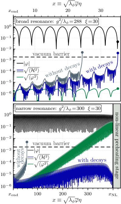
Figure 8: Evolution of the conformal variance for the Higgs $\langle\mathcal{H}^{2}\rangle$ and inflaton $\langle\varphi^{2}\rangle$, with their backreaction on the system included through the one-loop Hartree approximation. If the variance grows to the extent that $\omega_{\mathcal{H}_{k}}^{2}$ is dominated by the (negative) $3\lambda_{h}\langle\mathcal{H}^{2}\rangle$ term, the Higgs experiences a runaway tachyonic growth that rapidly destabilizes the electroweak vacuum, causing the sharp divergence in the curves. A point marker at the end of a curve indicates destabilization, and the gray curves show $\langle\mathcal{H}^{2}\rangle$ in the absence of decays. Identically to Fig. 4, the top (bottom) panels correspond to broad (narrow) parametric resonance, respectively. In the latter, $\langle\varphi^{2}\rangle$ grows sufficiently to end the linear preheating stage at $x_{\rm NL}\approx 400$, consistent with lattice results in the literature Khlebnikov and Tkachev (1996).

In the above, we have established a clear criterion for model viability: for a given choice of couplings, if the electroweak vacuum survives for a duration longer than $x_{\rm NL}$, then it survives the linear stage of preheating. The transient non-linear stage that follows tends to asymptote to thermal equilibrium, during which resonant particle production stops and the energy density is redistributed among the modes to approach a thermal distribution. We expect that if metastability is maintained until $x_{\rm NL}$ then it also survives the non-linear stage; we briefly discuss these issues and how massless preheating contrasts with other scenarios in the conclusions in Sec. V.

Our task then shifts to calculating the vacuum decay times $x_{\rm dec}$ as a function of the model parameters. A robust method to conservatively estimate $x_{\rm dec}$ is as follows Ema et al. (2016); Enqvist et al. (2016). As the Higgs fluctuations grow, the effective mass term associated with the Higgs self-interaction $3\lambda_{h}\langle h^{2}\rangle$ becomes negative and large enough to make some Higgs modes tachyonic over a time interval $\Delta t$. These modes grow exponentially in this interval at a rate $\sqrt{3|\lambda_{h}|\langle h^{2}\rangle}$. In turn, this amplifies $\langle h^{2}\rangle$, which then makes the tachyonic masses even larger—i.e., the system enters a positive feedback loop which rapidly destabilizes the vacuum. We can estimate $x_{\rm dec}$ as the time at which the growth exponent becomes larger than $\mathcal{O}(1)$:

$$\sqrt{\frac{3\langle h^{2}\rangle}{\overline{\phi}{}^{2}}\frac{|\lambda_{h}|}{\lambda_{\phi}}}\,\Delta x~{}\gtrsim~{}1\ ,$$ (66)

and we have used that $\Delta t=\Delta x/(\sqrt{\lambda_{\phi}}\,\overline{\phi})$.

Alternatively, in situations where the Higgs modes oscillate slowly relative to the background inflaton field, the simpler condition $3\lambda_{h}\langle h^{2}\rangle\gtrsim m_{h}^{2}$ is appropriate, in which we evaluate the effective Higgs mass $m_{h}$ [of Eq. (54)] at the amplitude of the inflaton oscillations $\phi=\overline{\phi}$.

The process of vacuum destabilization as it unfolds is illustrated in Fig. 8 by including backreaction in our numerical calculations. The panels reflect the same parameter choices made for Fig. 4 in the previous section, where we focus on the broad $g^{2}/\lambda_{\phi}=2n^{2}$ and narrow $g^{2}/\lambda_{\phi}=2n^{2}+n$ parametric resonances within the same coupling band (with $n=12$). The curvature coupling $\xi=30$ is subdominant but non-negligible. Both the Higgs and inflaton variance are shown, and the former shows the results both with (blue) and without (gray) Higgs decays. In the top panel, the perturbative decays delay destabilization but it ultimately occurs at $x_{\rm dec}\approx 35$. The runaway growth of the Higgs fluctuations is observed toward the endpoint of each curve, as they finally cross the vacuum barrier $\langle\mathcal{H}^{2}\rangle\geq(ah_{\rm crit})^{2}$. By contrast, in the lower panel we see that the narrow resonance would lead to destabilization in the absence of decays, after not much longer $x_{\rm dec}\approx 55$. However, we see that accounting for perturbative decays prevents vacuum destabilization. Moreover, we observe the onset of the non-linear stage at $x_{\rm NL}$ induced by the growth of inflaton fluctuations, as $\langle\varphi^{2}\rangle$ grows sufficiently large. As expected, this stage occurs at $x_{\rm NL}\approx 400$.

Let us now survey $x_{\rm dec}$ over the parameter space of couplings and produce analytical estimates in each region. We shall work largely in parallel to Sec. III and employ the results from that section. That is, we shall first cover the $\xi=0$ and $g=0$ limits separately and then progress to the mixed case, providing a general picture of vacuum metastability at the end of the section.

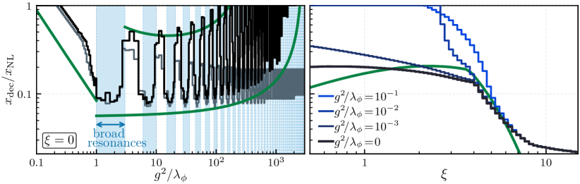
Figure 9: The decay time $x_{\rm dec}$ of the electroweak vacuum as a function of $g^{2}/\lambda_{\phi}$ (left panel) and $\xi$ (right panel), normalized by the onset time $x_{\rm NL}$ of the non-linear stage. The vacuum survives preheating for $x_{\rm dec}\geq x_{\rm NL}$. In the left panel, the results are shown both with (black curve) and without (gray curve) perturbative Higgs decays. Our analytical estimates in this panel (green curves) correspond to the different regimes of Eq. (69). In particular, the two green curves for $g^{2}/\lambda_{\phi}\gtrsim 1$ show the broad and narrow regimes, evaluated using $\mu_{\rm max}\approx 0.24$ and Eq. (30), respectively. As these $\mu_{\rm max}$ correspond to the minimum and maximum growth exponents, they estimate the envelope of the highly non-monotonic $x_{\rm dec}$. In the right panel, the analytical estimates are also shown by green curves and correspond to Eq. (71) and Eq. (72), plotted over their regions of validity.

IV.2.1 From Parametric Instability

Let us first consider destabilization of the vacuum from the parametric resonance. The effective mass of a Higgs mode $\omega^{2}_{h_{k}}\approx k^{2}/a^{2}+g^{2}\phi^{2}+3\lambda_{h}\langle h^{2}\rangle$ may first become tachyonic once the inflaton field passes through $\phi=0$. We can estimate $x_{\rm dec}$ by following the discussion surrounding Eq. (66), but we must first calculate the Higgs variance. Using that $\langle h^{2}\rangle\simeq n_{h}/(a^{3}\omega_{h})$, with Eq. (31) and Eq. (51) for the different coupling regimes, we find

$$\langle h^{2}\rangle~{}\simeq~{}\begin{cases}\displaystyle{\frac{\lambda_{\phi}\overline{\phi}{}^{2}}{T^{3/2}}\sqrt{\frac{\mu_{\rm max}}{2x}}e^{2\mu_{h}x}}&\text{for }g^{2}/\lambda_{\phi}\lesssim 1\\[6.0pt] \displaystyle{\frac{\lambda_{\phi}\overline{\phi}{}^{3}}{16\pi^{3}\left|\phi\right|}\left(\frac{g^{2}}{8\lambda_{\phi}}\right)^{\!\!\frac{1}{4}}\!\frac{e^{2\mu_{h}x}}{\sqrt{\mu_{\rm max}x}}}&\text{for }g^{2}/\lambda_{\phi}\gtrsim 1\end{cases}\ ,$$ (67)

where we have defined the effective rate

$$\mu_{h}~{}\equiv~{}\mu_{\rm max}-\frac{1}{2\gamma}\frac{\left\langle a\Gamma_{h}\right\rangle}{\sqrt{\lambda_{\phi}}\overline{\varphi}}$$ (68)

in terms of the conformal decay rate of Eq. (56). The Lorentz factor $\gamma\simeq\max(1,\sqrt{\lambda_{\phi}/g^{2}})$ accounts for the dilation of relativistic Higgs decays, which is negligible in the $g^{2}/\lambda_{\phi}\gtrsim 1$ regime but important for $g^{2}/\lambda_{\phi}\lesssim 1$. Finally, the vacuum decay time is found in both regimes:

$$x_{\rm dec}\simeq\hskip 0.85358pt\begin{cases}\displaystyle{\frac{-1}{4\mu_{h}}W_{-1}\left[\frac{-9\lambda_{h}^{2}}{32\pi^{2}}\frac{F_{1}^{2}\mu_{h}}{T\mu_{\rm max}}\right]}&\!\!\!\text{for }g^{2}/\lambda_{\phi}\lesssim 1\\[9.0pt] \displaystyle{\frac{-1}{4\mu_{h}}W_{-1}\left[\frac{-9\lambda_{h}^{2}}{(2\pi)^{6}}\frac{\mu_{h}}{\mu_{\rm max}}\right]}&\!\!\!\text{for }g^{2}/\lambda_{\phi}\gtrsim 1\end{cases}\,.$$ (69)

The $g^{2}/\lambda_{\phi}\gtrsim 1$ result is based on the destabilization condition in Eq. (66). Meanwhile, for $g^{2}/\lambda_{\phi}\lesssim 1$ the Higgs modes oscillate slowly relative to the inflaton background, so that $3\lambda_{h}\langle h^{2}\rangle\gtrsim g^{2}\overline{\phi}{}^{2}$ is an appropriate condition. Additionally, note that $\mu_{\rm max}$ depends on the regime of the resonance, as given explicitly in Sec. III.1.

Manifestly, the effective rate $\mu_{h}$ shows the competition between particle production and decays. For large enough coupling, the decays can eventually dominate, because $\mu_{\rm max}$ is globally bounded from above; the decay rate of produced Higgs particles scales with the coupling, but the rate of particle production does not.

Let us compute the critical value of the coupling for which $x_{\rm dec}\geq x_{\rm NL}$, i.e., the smallest coupling for which the metastable vacuum survives preheating. We shall separately consider the couplings corresponding to the broad and narrow resonances. In the broad regime, we find $g^{2}/\lambda_{\phi}\gtrsim 2.4\times 10^{3}$. Likewise, using Eq. (30) for $\mu_{\rm max}$, for the narrow resonances we find $g^{2}/\lambda_{\phi}\gtrsim 213$. The dramatic gap between these thresholds reflects the difference in the strength of the resonance between these two regimes. Indeed, confirming our earlier observations in Eq. (57), we find that perturbative decays of the Higgs stabilize the electroweak vacuum for sufficiently large quartic couplings, and these couplings significantly differ based on the regime of the parametric resonance.

To paint a more complete picture and confirm our analytical results, we solve the mode equations numerically within the one-loop Hartree approximation and scan continuously over the range of couplings $g^{2}/\lambda_{\phi}$; this is shown in the left-hand panel of Fig. 9. The black and gray curves show the numerical results with and without perturbative decays, respectively. In line with our calculations in Eq. (69), we find that $x_{\rm dec}$ is highly non-monotonic with respect to the quartic coupling. Indeed, this behavior originates from the structure of the resonance bands (in Fig. 2), in which the minima (maxima) of the oscillations correspond to the broad (narrow) resonance regimes, respectively. Therefore, evaluating our analytical result in Eq. (69) at the broad and narrow $\mu_{\rm max}$ values estimates the envelope of the $x_{\rm dec}$ oscillations. This envelope is shown by the thick green curves at $g^{2}/\lambda_{\phi}\geq 1$ in Fig. 9. We also show our analytical estimate for the $g^{2}/\lambda_{\phi}\leq 1$ region. Meanwhile, the pivotal role of the perturbative decays is highlighted by the gray curve, which shows the numerical $x_{\rm dec}$ with perturbative decays turned off. Indeed, in the absence of decays, the vacuum is stabilized only for very small coupling $g^{2}/\lambda_{\phi}\lesssim 0.25$.

IV.2.2 From Tachyonic Instability

Likewise, let us consider the pure curvature coupling limit, in which $g=0$. We once again confine our discussion to $\xi>0$ since otherwise the vacuum decays. From Sec. III, we know that the growth of fluctuations from this tachyonic source is very different from the parametric instability. Most notably, the tachyonic production ceases once $x\gtrsim x_{\xi}$, even for the zero mode. We estimate the variance again using $\langle h^{2}\rangle\simeq n_{h}/(a^{3}\omega_{h})$, and since the effective mass is curvature dominated we have $\omega_{h_{k}}^{2}\simeq\xi R\simeq\xi\lambda_{\phi}\overline{\phi}{}^{4}$. Using Eq. (37) then yields

$$\langle h^{2}\rangle~{}\simeq~{}\frac{3^{15/8}}{8}\frac{\xi^{1/4}\lambda_{\phi}\overline{\phi}{}^{4}}{(8\pi)^{3/2}}\left(\frac{x}{x_{0}}\right)^{\!\!4\sqrt{\frac{2\xi}{3\sqrt{3}}}}$$ (70)

for $x<x_{\xi}$. Afterward, there is no particle production, so $n_{h}$ is fixed and $\omega_{h}\propto\overline{\phi}{}^{2}\propto 1/a^{2}$. The variance then redshifts as $\langle h^{2}\rangle\approx n_{h}/(a^{3}\omega_{h})\propto 1/a$, which is slower than the scaling one would find in the quartic-dominated case.

The fact that $\langle h^{2}\rangle$ redshifts in this way is a crucial observation. If the ratio $\langle h^{2}\rangle/h_{\rm crit}^{2}$ grows at times $x\gtrsim x_{\xi}$ due to its redshifting behavior, the vacuum may decay even after particle production shuts down. For the quartic interaction, this ratio would be fixed. However, for the curvature interaction, the variance redshifts more slowly $\langle h^{2}\rangle\propto 1/a$, and the barrier redshifts more rapidly $h_{\rm crit}^{2}\simeq\xi_{h}R/|\lambda_{h}|\propto 1/a^{4}$. Consequently, the ratio redshifts as $\langle h^{2}\rangle/h_{\rm crit}^{2}\propto a^{3}$ and grows. Even if the Higgs remains stable throughout the tachyonic phase, it destabilizes once the fluctuations grow beyond the extent of the barrier $\langle h^{2}\rangle\gtrsim h_{\rm crit}^{2}$; this leads to a vacuum decay at

$$x_{\rm dec}~{}\simeq~{}\frac{8\sqrt{\pi}\xi^{3/4}}{3^{1/8}|\lambda_{h}|^{1/3}}\left(\frac{x_{0}}{x_{\xi}}\right)^{\!\!\frac{4}{3}\!\sqrt{\!\frac{2\xi}{3\sqrt{3}}}}\ ,$$ (71)

which is valid for $x_{\rm dec}>x_{\xi}$, or equivalently $\xi\lesssim 16$. Note that the presence of even a small quartic coupling may shield the vacuum from this effect, since the quartic term will eventually dominate $g^{2}\phi^{2}\gtrsim\xi R$ and halt the growth of $\langle h^{2}\rangle/h_{\rm crit}^{2}$, which happens once $x\gtrsim\sqrt{12\xi\lambda_{\phi}/g^{2}}$.

Otherwise, destabilization occurs during the tachyonic phase and the condition in Eq. (66) can be used again to produce an estimate. This task is now more complicated since backreaction is not the only source of tachyonicity. The vacuum could decay in one of two ways: (i) by the $3\lambda_{h}\langle h^{2}\rangle$ term or (ii) directly by the tachyonic mass of the curvature term. A coupling of order $\xi\gtrsim\mathcal{O}(10)$ is sufficient to produce the latter, and in this case the vacuum decays rapidly. For smaller $\xi$, however, the false vacuum can survive much longer. Using Eq. (66) with the approximation that $\Delta x\simeq T/2$ leads to

$$x_{\rm dec}~{}\simeq~{}\frac{256\sqrt{2}\pi^{3/2}\xi^{3/4}}{9\cdot 3^{7/8}|\lambda_{h}|T^{2}}\left(\frac{x_{\xi}}{x_{0}}\right)^{\!\!1-4\sqrt{\!\frac{2\xi}{3\sqrt{3}}}}\ .$$ (72)

We consider this result consistent with our assumptions only if Eq. (72) gives an earlier decay time than Eq. (71); in terms of the curvature coupling, this implies a region of validity $\xi\gtrsim 4$ for Eq. (72).

Our numerical computations of the vacuum decay time $x_{\rm dec}$ are shown in the right panel in Fig. 9. The pure curvature coupling case corresponds to the black curve and the analytical estimates constitute the thick green curve. We have also included the numerical results for several small quartic couplings in the range $10^{-3}\lesssim g^{2}/\lambda_{\phi}\lesssim 10^{-1}$. These results are in line with our rough estimates and confirm that the presence even of a small quartic coupling can prevent decay of the false vacuum. We have neglected $\xi\gtrsim\mathcal{O}(10)$ in our analytical estimates since these correspond to rapid destabilization, for which the precise values of $x_{\rm dec}$ are not essential.

IV.2.3 The Mixed Case

Let us finally consider the general mixed case in which both couplings $\xi$ and $g^{2}/\lambda_{\phi}$ are non-zero. As we have observed in Sec. III.3, if the strength of the curvature coupling is at least comparable to $g^{2}/\lambda_{\phi}$ the system undergoes a sequence of distinct phases of particle production. In the context of vacuum stability, this means that the electroweak vacuum must initially survive a phase of tachyonic production until $x_{\xi}\simeq[6\xi/\sqrt{g^{2}/\lambda_{\phi}}]^{1/2}$ and then survive the parametric instability until non-linear dynamics set in at $x_{\rm NL}$. In what follows below, we shall assume such a scenario for our analytical calculations.

Rather than concern ourselves directly with $x_{\rm dec}$, we produce an estimate of the constraint for vacuum metastability by examining where $\langle h^{2}\rangle\gtrsim h_{\rm crit}^{2}$. In the $\xi>0$ region we can write $\langle h^{2}\rangle$ using Eq. (44) together with $\langle h^{2}\rangle\simeq n_{h}/(a^{3}\omega_{h})$. We arrive at the expression

$$\langle h^{2}\rangle~{}\simeq~{}\frac{\lambda_{\phi}\overline{\varphi}}{8\pi^{3}\sqrt{\xi}}\left(\frac{T}{2x}\sqrt{\frac{g^{2}}{2\lambda_{\phi}}}\right)^{\!\!\!3/2}\!\!e^{\frac{12\sqrt{2}\pi\xi}{T\sqrt{\!g^{2}/\lambda_{\phi}}}\left(\!\frac{1}{x_{0}}-\frac{1}{x}\!\right)}\ .$$ (73)

Owing to the exponential growth of $\langle h^{2}\rangle$, the constraint on our parameter space has only a logarithmic sensitivity to $h_{\rm crit}^{2}$ and the coefficient in Eq. (73). That said, the constraint is sensitive to the rate of perturbative decays, and we should reintroduce this rate as we calculate our result. Along these lines, we find

$$\xi~{} \lesssim~{}\frac{x_{0}T}{12\sqrt{2}\pi}\sqrt{\frac{g^{2}}{\lambda_{\phi}}}\left[\log\mathcal{C}_{+}+\frac{\left\langle a\Gamma_{h}\right\rangle}{\sqrt{\lambda_{\phi}}\overline{\varphi}}x_{\rm dec}\right]\ ,$$ (74)

where all of the logarithmic terms have been collected into the quantity $\log\mathcal{C}_{+}$. The dependence on $x_{\rm dec}$ and $\langle a\Gamma_{h}\rangle$ are important. To manage $x_{\rm dec}$, a natural assumption is that $x_{\rm dec}\lesssim x_{\xi}$ in the region we are evaluating, since otherwise the tachyonic effect is not strong enough to destabilize the vacuum. We therefore have at most $x_{\rm dec}\simeq(6\xi/\sqrt{g^{2}/\lambda_{\phi}})^{1/2}$. We can solve the more complicated inequality that results for $\xi$ (and we shall do this numerically below), but based on our observations of the tachyonic effect in this section $x_{\rm dec}=\mathcal{O}(10)$ serves as an appropriate simplifying approximation. As discussed in Sec. III.4, the perturbative decays arising from the quartic interaction are generally more relevant, and these scale parametrically as $\Gamma_{h}\propto\sqrt{g^{2}/\lambda_{\phi}}$. These considerations lead to a constraint of roughly $\xi\lesssim\mathcal{O}(0.1)g^{2}/\lambda_{\phi}$ to ensure metastability.

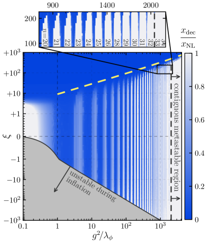
Figure 10: The decay time $x_{\rm dec}$ of the electroweak vacuum computed numerically and normalized by $x_{\rm NL}$. The gray region is excluded due to violating Eq. (11). The white regions show “islands of (meta)stability” in which the false vacuum survives preheating. Along the $g^{2}/\lambda_{\phi}$ direction, the pattern reflects the band structure in Sec. III.1, with the least stable regions centered around $g^{2}/\lambda_{\phi}=2n^{2}$ (for $n\in\mathbb{N}$). For larger $g^{2}/\lambda_{\phi}$, perturbative Higgs decays enlarge the metastable regions until they become contiguous at $g^{2}/\lambda_{\phi}\gtrsim 2\times 10^{3}$ [in agreement with Eq. (69)]. The effect of the curvature interaction is to form an envelope over the metastable regions, and the yellow curve shows our estimate [from Eq. (74)] for $\xi>0$.

An interesting feature of the mixed-coupling scenario is that it opens the possibility of metastability in the $\xi<0$ region, which is ruled out if $g^{2}/\lambda_{\phi}=0$. A similar procedure to the above is followed to produce a bound on the $\xi<0$ region, the details of which are included in Appendix B. The constraint is expressed as

$$\hskip-9.10509pt-\xi-\xi_{\phi}\frac{g^{2}}{\lambda_{\phi}}\lesssim\frac{\small\log\mathcal{C}_{-}-\frac{\sqrt{6}H_{1}(3,0)}{3T\sqrt{-\xi}}\frac{g^{2}}{\lambda_{\phi}}(x_{\rm dec}^{2}-x_{0}^{2})+(x_{\rm dec}-x_{0})\frac{\langle a\Gamma_{h}\rangle}{\sqrt{\lambda_{\phi}}\overline{\varphi}}}{\frac{8}{T}\sqrt{\frac{6}{-\xi}}H_{1}(3,0)\log\!\big{(}\frac{x_{\rm dec}}{x_{0}}\big{)}},$$

(75)

and we have again taken $x_{\rm dec}=\mathcal{O}(10)$ and packaged the logarithmic terms in a quantity $\mathcal{C}_{-}$. The function giving $H_{1}(3,0)\approx 0.76$ is defined in Appendix B. Note that for $\xi\gg 1$ the term proportional to $g^{2}/\lambda_{\phi}$ on the left-hand side is subdominant and the remaining terms balance for $|\xi|\sim g^{2}/\lambda_{\phi}$. Therefore, neglecting numerical coefficients, the constraint becomes $\xi\lesssim\mathcal{O}(g^{2}/\lambda_{\phi})$. The negative curvature coupling thus yields a weaker bound, which is expected based on our observations from Sec. III.3. Note that the inflation constraint $\xi_{h}-\xi_{\phi}g^{2}/\lambda_{\phi}\gg 1/12$ in Eq. (11) yields a bound that is roughly coincident.

A more complete picture of the constraints is achieved by numerical calculations, and we display these in Fig. 10. For this figure, we have calculated the time of vacuum decay $x_{\rm dec}$ over the $\{g^{2}/\lambda_{\phi},\xi\}$ parameter space, making the simplifying assumption that $\xi_{\phi}=0$. Note that the gray region excludes the subset of couplings that destabilizes the vacuum during inflation. Additionally, note that the curvature coupling is shown on a log scale over the negative and positive axes, with the exception of the range $-1\leq\xi\leq+1$ where the scale is linear. The numerics run until a time $x_{\rm NL}$ so that the white regions effectively show where $x_{\rm dec}/x_{\rm NL}\geq 1$ and thus where the vacuum remains metastable throughout preheating.

Echoing the behavior observed in Fig. 9, we find that over the vast majority of parameter space, the metastable regions are not connected. Instead, we find a large number of disjoint “islands of (meta)stability” scattered throughout. Indeed, the constraint for metastability cannot be fully expressed as a simple bound on the couplings—the fate of the electroweak vacuum depends on $g^{2}/\lambda_{\phi}$ in a highly monotonic way. Naturally, the most unstable regions appear where the characteristic exponent $\mu_{\rm max}$ is maximized—i.e., around the broad resonances $g^{2}/\lambda_{\phi}=2n^{2}$ (for $n\in\mathbb{N}$). Conversely, the most stable regions appear around the narrow resonances, where $\mu_{\rm max}$ is minimized [see Eq. (30)]. As $g^{2}/\lambda_{\phi}$ is taken to larger values, the metastable regions grow and start to merge, as shown by the magnified inset panel. The integers written over the metastable regions correspond to the couplings of the narrow resonances written in the form $g^{2}/\lambda_{\phi}=2n^{2}+n$. The couplings eventually become large enough for perturbative decays to stabilize the Higgs, regardless of the resonance regime, forming a contiguous metastable region for $g^{2}/\lambda_{\phi}\gtrsim 2\times 10^{3}$. This observation agrees with our analytical estimates in Eq. (57) and Eq. (69) for the broad regime. In principle, the only limitation in taking larger couplings is that we do not ruin the flatness of the inflaton potential, which (as briefly discussed in Sec. II.1) roughly requires $g^{2}/\lambda_{\phi}\ll 10^{5}$.

Beyond these observations, we notice that the interplay of the couplings is also clarified in Fig. 10. In particular, the figure shows that the Higgs-curvature interaction has the effect of cutting off the metastable regions and imposing an envelope that scales with the couplings. This envelope is what we have analytically estimated in Eq. (74) and Eq. (75). We have plotted the numerical solution to the inequality in Eq. (74) using a yellow-dashed curve. This curve is indeed consistent with the approximate bound that we estimated $\xi\lesssim\mathcal{O}(0.1)g^{2}/\lambda_{\phi}$. We have not included the analogous curve for the $\xi<0$ region since this closely coincides with the constraint (the gray region) on the stability of the vacuum during inflation. On the whole, the interplay between the two interactions effectively extends the range of metastability for the Higgs-curvature coupling, shielded by the presence of a similarly large Higgs-inflaton coupling.

V Conclusions and Discussion

Some amount of degeneracy often exists in inflationary models in the sense that observational constraints may be satisfied over a degenerate subspace of the model parameters. Undoubtedly, one reason that studies of post-inflationary dynamics are essential is that this dynamics may break such degeneracies by leading to qualitatively different preheating histories, subject to a qualitatively different set of possible constraints. For example, as we have encountered in this paper, the stability of the Higgs during inflation can be ensured by either a direct coupling to the inflaton or a non-minimal coupling to gravity. The dynamical roles played by these interactions are similar during inflation but differ dramatically during preheating, in which the non-trivial interplay between these interactions implies a rich structure of metastable regions and associated constraints on the Higgs couplings. Indeed, the broader motivation for this work is to explore dynamics that may reveal independent probes for models of early-universe cosmology.

In this paper, we have examined the massless preheating dynamics that arises in models composed of scale-invariant interactions, in which the inflaton potential is effectively quartic after inflation. Most notably, we have focused on the implications these models have for electroweak vacuum metastability. We have provided constraints on the couplings for which the Higgs remains stabilized during and after inflation. Among these couplings, we have included the possibility that the Higgs and the inflaton have non-minimal couplings to gravity. While our study is motivated by addressing the metastability of the vacuum, our results are readily generalized to other approximately scale-invariant models.

Several comments are in order. First, while we have considered non-minimal gravitational couplings for both the Higgs and inflaton fields, the Higgs coupling $\xi_{h}$ has received the bulk of our attention. And while the effects of $\xi_{\phi}$ have been included in our analysis through the effective curvature coupling $\xi$ [in Eq. (27)], our treatment can be extended in several ways. For example, we have not taken into account the higher-order effects on the field fluctuations that appear as a result of $\xi_{\phi}\neq 0$ corrections to the background-field solutions. For this reason, our results are applicable only for $|\xi_{\phi}|\lesssim 1$, which is the scope assumed for this paper. These higher-order effects are challenging to incorporate analytically in massless preheating. Notably, even the zeroth-order background solution [the elliptic function in Eq. (16)] is considerably more complicated than the sinusoidal form found in massive preheating. It would be worthwhile to study the effects of $\xi_{\phi}\approx-\mathcal{O}(1)$ without resorting to such approximations for the background equations of motion.

Second, our study is performed under the assumption that there is no new physics beyond the SM that significantly alters the renormalization-group evolution of the Higgs quartic coupling. This assumption could be reasonable, as there are no hints of new physics in collider or weakly interacting massive particle dark-matter searches. Either way, the cosmological history following the preheating stage—i.e., the reheating epoch and, more precisely, the inflaton decay channels—should be consistent with this assumption. The reheating epoch could then be realized in a number of ways. For instance, the inflaton could couple to the right-handed neutrino, which is responsible for neutrino masses and leptogenesis Fukugita and Yanagida (1986). In this case, reheating could be completed by the decay of inflaton to right-handed neutrinos and their subsequent decay to SM particles. Alternatively, if the inflaton is stable, it also opens the possibility that the inflaton is a candidate for dark matter Almeida et al. (2019); Lebedev and Yoon (2021) or dark radiation Babichev et al. (2020), provided that preheating converts most of the inflaton energy density into SM degrees of freedom. Indeed, the details and variations on these possibilities ultimately depend on the sign and size of the inflaton mass-squared term.

Along another direction, some comments are in order regarding the stage of preheating that occurs after $x_{\rm NL}$ in our study. After entering the non-linear stage of preheating, the energy density held in fluctuations is redistributed among the modes by rescattering processes. In general, the Higgs can destabilize during this time, and this possibility has been addressed for massive preheating in Ref. Ema et al. (2016), based on the results of Refs. Harigaya and Mukaida (2014); Mukaida and Yamada (2016). In massive preheating, this destabilization arises because the effective Higgs mass induced by the inflaton-Higgs coupling redshifts as $g^{2}\phi^{2}\propto 1/a^{3}$, while that induced by the Higgs self-coupling redshifts as $3\lambda_{h}\langle h^{2}\rangle\propto 1/a^{2}$. In other words, the tachyonic contribution continues to grow relative to the stabilizing mass term and can eventually trigger decay of the vacuum, even though it was stabilized at the end of the linear preheating stage. The details of the thermal Higgs mass after preheating and the evolution of the background temperature thus become important to ensure metastability as thermalization begins. That said, in massless preheating, these two mass contributions redshift at the same rate $g^{2}\phi^{2}\sim 3\lambda_{h}\langle h^{2}\rangle\sim 1/a^{2}$, so these same concerns over destabilization are not as relevant. Nevertheless, the stages of evolution leading to thermalization are, of course, interesting in the context of massless preheating for a host of other reasons. Furthermore, other considerations such as the thermal corrections to the vacuum tunneling probability become important during the reheating epoch, such as those studied in Ref. Delle Rose et al. (2016).

Thermal effects could be important even before $x_{\rm NL}$, through direct decay channels (if any) of the inflaton into SM particles or through the Higgs decay products. Whether the Higgs decay products become quickly thermalized is a nontrivial issue, since the particle-production rate can greatly exceed the thermalization rate. In this case, one may not necessarily assume that the Higgs decay products form a thermal plasma, even if the thermal relaxation time is much shorter than the age of the Universe at that moment. Nevertheless, if instant thermalization of the decay products is assumed, we can discuss thermal backreaction on the Higgs dynamics. If the thermal mass of the Higgs becomes comparable to the zero-temperature effective mass, our analysis would be modified, and we would expect broader regions in Fig. 10 to become (meta)stable. Our preliminary study shows that the effect of the Higgs thermal mass is insignificant over a wide range of the parameter space. However, it is important to correctly account for the full evolution of the decay products without the thermalization assumption, which we leave for future work.

As we recall from Sec. IV.1, the time $x_{\rm NL}$ at which the non-linear stage of preheating begins is central to our results. We concluded, in our minimal model realization, that the inflaton self-resonance is responsible for the onset of the non-linear stage, as its fluctuations grow from the quartic self-resonance. However, a natural extension is to consider the presence of a spectator field that does not couple to the Higgs. If such a spectator field is likewise subject to particle production, then $x_{\rm NL}$ could be triggered by the growth of the spectator fluctuations instead; this is not difficult to arrange, considering that the characteristic exponent for the inflaton self-resonance is rather small at $\mu_{\rm max}\approx 0.036$. A reduction in $x_{\rm NL}$ would imply that our metastable regions, such as those that appear in Fig. 10, grow in extent. This enhancement could be substantial. For example, taking a quartic coupling between the spectator and the inflaton, with the maximal exponent $\mu_{\rm max}\approx 0.24$, we find that $x_{\rm NL}\approx 63$, roughly a factor of 6 smaller than the inflaton self-resonance.

Moreover, the possibility of spectator fields opens other avenues of exploration. For instance, such fields could generate important cosmological observables such as non-Gaussianities in the density perturbations Chambers and Rajantie (2008). Additionally, spectator fields could naturally serve as dark-matter candidates. The corresponding relic abundance generated from preheating would depend non-trivially on the couplings and spins of the spectator fields. It is worth noting that such dark-matter production from the thermal bath with a generic equation of state—including the radiation-like equation of state relevant to our study—has been a topic of recent interest Garcia et al. (2020, 2021).

There are also a number of possible extensions that would be interesting to explore in the context of multi-field inflation. For instance, in models which allow for a sizeable angular inflaton velocity at the end of inflation Cline et al. (2020); Kawasaki and Ueda (2021), the inflaton-dependent modulation of the effective Higgs masses could be suppressed. As a result, the rate of particle production could be suppressed as well. On the other hand, the onset of the non-linear stage of preheating would also occur at a later time $x_{\rm NL}$. The end result of the competition between these two effects, and the more complicated preheating dynamics altogether, requires a dedicated study Kost et al. . An alternative multi-field extension could involve hybrid inflation Linde (1994). In this case, vacuum stability during inflation is ensured by the inflaton-Higgs coupling as usual, but this coupling will not oscillate much during the preheating phase since most of the energy is transferred to the so-called waterfall fields Garcia-Bellido and Linde (1998). These features imply that the electroweak vacuum would be relatively stable during both inflation and preheating.

It would also be interesting to consider the presence of additional terms that break the scale invariance of the theory, as these can have rich dynamical implications. While the breaking of the scale invariance due to the non-minimal coupling terms are relevant only around the end of inflation, effects of lower-dimensional terms become more and more important at a later time. For instance, a non-vanishing inflaton mass $m_{\phi}$ might alter the parametric resonance once the inflaton oscillations reach a sufficiently small amplitude Greene et al. (1997). In particular, for couplings $g^{2}/\lambda_{\phi}\gtrsim\lambda_{\phi}/m_{\phi}^{2}$ the resonance becomes stochastic once $\overline{\phi}\lesssim m_{\phi}/\!\sqrt{\lambda_{\phi}}$. The parametric resonance then increasingly behaves as in massive preheating (see Appendix A), with the stochastic resonance giving way to the narrow resonance once $\bar{\phi}\lesssim m_{\phi}/g$. Not only does this evolution change the spectrum of produced particles and the production rates, the introduction of $m_{\phi}\neq 0$ also allows the resonance to terminate at some time before $x_{\rm end}$. A small inflaton mass can thus modify our constraints for electroweak metastability in a non-trivial way.

Yet another possible extension of our work concerns the gravity formulation. In this paper, given the non-minimal couplings of our scalar fields to gravity, we have observed some of the physical distinctions that may appear between the metric and Palatini formulations. Still, a more general extension could be explored along the lines of the Einstein-Cartan formulation in the presence of Holst and Nieh-Yan terms Shaposhnikov et al. (2021a, 2020, b). The Einstein-Cartan theory generalizes our treatment, reproducing the metric and Palatini formulations in certain limits and allowing for a continuous interpolation between them.

All in all, if the metastability of the electroweak vacuum may be ensured in models from which massless preheating emerges, we may adopt a renewed interest in observables that are sensitive to the details of preheating. A well-suited example consists of gravitational waves (GWs) produced during this epoch Figueroa and Torrenti (2017). Massless preheating is distinctive in this sense because the amplitude of the produced gravitational radiation does not dissipate and the frequency of the waves does not redshift. While these properties may present challenges for the observational prospects of GWs from such scenarios, several methods show promise Aggarwal et al. (2020). For example, radio telescopes may be used to examine the distortion in the CMB from by-products of high-frequency GWs interacting with background magnetic fields Domcke and Garcia-Cely (2021). Indeed, such observations could even be used to probe broader early-universe properties, such as the energy scale for inflation Cai et al. (2022).

Appendix A Comparison to Massive Preheating

In this appendix, we provide a brief overview of the “massive preheating” dynamics, in which our Lagrangian takes the same form as Eq. (II), but the potential is instead given in the Jordan frame by

$$V_{\rm J}(\phi,h)~{}=~{}\frac{1}{2}m_{\phi}^{2}\phi^{2}+\frac{1}{2}g^{2}\phi^{2}h^{2}+\frac{1}{4}\lambda_{h}h^{4}\ ,$$ (76)

where $m_{\phi}$ is the inflaton mass. Note that previous studies in the literature have examined electroweak vacuum metastability for this model in the $\xi_{\phi}=0$ limit Ema et al. (2016, 2017), and we refer the reader to those papers for details beyond the scope of our summary.

All other features of the model beyond the mass term are assumed to remain the same. After the end of inflation, when $|\xi_{\phi}|\phi^{2}\ll 1$ the inflaton potential is approximately quadratic and the field evolves according to

$$\ddot{\phi}+3H\dot{\phi}+m_{\phi}^{2}\phi~{}=~{}0\ .$$ (77)

The inflaton amplitude then redshifts as $\overline{\phi}\propto 1/a^{3/2}$ and [in line with Eq. (18)] the cosmological equation of state is matter-like. The inflaton field evolution is sinusoidal:

$$\varphi(x)~{}=~{}\overline{\varphi}\cos(x-x_{0})\ ,$$ (78)

where in analogy to Sec. II.2 we have defined $\varphi=a^{3/2}\phi$ and the dimensionless time $x\equiv mt$. The constant $x_{0}$ is fixed by the conditions at the end of inflation, and we shall assume $\phi_{\rm end}=\mathcal{O}(1)$. The scale factor evolves as

$$a(x)~{}=~{}\frac{1}{2}\big{(}\sqrt{3}\overline{\varphi}x\big{)}^{\!2/3}$$ (79)

and thus for consistency $x_{\rm end}=2\sqrt{2/3}\phi_{\rm end}^{-3/2}$.

To compute the growth of fluctuations we write the equations of motion for the Higgs modes in the Einstein frame. By defining $\mathcal{H}_{k}\equiv a^{3/2}\Omega^{-1/2}|_{h=0}h_{k}$, we can remove the damping terms, and up to $\mathcal{O}(a^{-3})$ we have

$$\mathcal{H}_{k}^{\prime\prime}+\omega_{\mathcal{H}_{k}}^{2}\mathcal{H}_{k}~{}=~{}0\ ,$$ (80)

in which the effective masses are

$$\omega_{\mathcal{H}_{k}}^{2}~{} =~{}\frac{\kappa^{2}}{a^{2}}+\Big{(}\frac{g^{2}}{m_{\phi}^{2}}+\xi_{h}\Big{)}\frac{\varphi^{2}}{a^{3}}+\xi\Big{(}\frac{\varphi^{2}}{a^{3}}-\frac{\varphi^{\prime 2}}{a^{3}}\Big{)}$$

$$=~{}\frac{\kappa^{2}}{a^{2}}+\frac{\overline{\varphi}{}^{2}}{a^{3}}\Big{[}\xi\sin^{2}(x-x_{0})$$ (81)

$$\hskip 62.59605pt+\Big{(}\frac{g^{2}}{m_{\phi}^{2}}+\xi+\xi_{h}\Big{)}\cos^{2}(x-x_{0})\Big{]}\ .$$

We have defined the rescaled momenta $\kappa\equiv k/m$, and in the second line we have employed Eq. (78). Additionally, in analogy to Eq. (27) we have defined the effective curvature coupling

$$\xi\equiv\xi_{h}+\xi_{\phi}-6\theta\xi_{h}\xi_{\phi}-\frac{3}{8}\ .$$ (82)

The rate of cosmological expansion is much smaller than that of the inflaton oscillations, so that the mode equations in Eq. (80) approximately take the Mathieu form $\mathcal{H}_{k}^{\prime\prime}+\{A_{k}-2q\cos[2(x-x_{0})]\}\mathcal{H}_{k}=0$, with the slowly varying parameters given by

$$A_{k}~{} \equiv~{}\frac{\kappa^{2}}{a^{2}}+\frac{\overline{\phi}{}^{2}}{2}\!\left(\frac{g^{2}}{m_{\phi}^{2}}+\xi_{h}\right)$$

$$q~{} \equiv-\frac{\overline{\phi}{}^{2}}{4}\!\left(\frac{g^{2}}{m_{\phi}^{2}}+2\xi+\xi_{h}\right)\ .$$ (83)

An important observation is that the contributions to the effective Higgs mass from the quartic interaction $g^{2}\phi^{2}\propto 1/a^{3}$ and non-minimal coupling $\xi_{h}R\propto 1/a^{3}$ redshift identically in the massive preheating scenario. Because much of the complexity we found in our study of massless preheating arose from the mismatch between these two terms, the massive preheating scenario is simpler in this respect. For example, whether particle production for a given mode occurs through the tachyonic or parametric instability is determined by the sign of $A_{k}-2|q|$. Namely, $A_{k}-2|q|>0$ yields the parametric instability, and $A_{k}-2|q|<0$ yields the tachyonic instability. We can write these explicitly as

$$A_{k}-2|q|~{}=~{}\frac{\kappa^{2}}{2}+\overline{\phi}{}^{2}\begin{cases}\left(-\xi\right)&\text{for }q<0\\ \left(\frac{g^{2}}{m_{\phi}^{2}}+\xi+\xi_{h}\right)&\text{for }q>0\end{cases}\ .$$ (84)

Therefore, unlike in the massless preheating scenario, the type of particle production that drives the zero mode is a fixed time-independent property based on the couplings. Notably, in the $g,\xi_{\phi}\rightarrow 0$ limit we recover the well-known result that $3/16<\xi_{h}<3/8$ is necessary for the complete absence of tachyonic production Ema et al. (2016).

Another crucial distinction between the massless and massive preheating dynamics is found by reexamining the perturbative Higgs decays. In particular, using the rest-frame decay rate $\Gamma_{h}$ in Eq. (53), the decays introduce a dissipative exponent $-\int dx\,\Gamma_{h}/\gamma$ that suppresses the growth of the Higgs number density. In terms of the Mathieu parameters the effective Higgs mass is given by $m_{h}^{2}=A_{0}-2q\cos[2(x-x_{0})]$ so that

$$-\int dx\,\Gamma_{h}~{}\propto~{}\int dx\sqrt{A_{0}-2q\cos{[2(x-x_{0})]}}\ ,$$ (85)

where the integration region is over the preheating times $x\geq x_{\rm end}$ for which $m_{h}^{2}\geq 0$ and we have taken $\gamma=1$. Because this integral has an identical form to the accumulated phase of the zero mode $\Theta_{0}$ [refer to the general quantity defined in Eq. (33)], we can employ previous calculations for $\Theta_{k}$ available in the literature Dufaux et al. (2006). The decay exponent amounts to a sum over each non-tachyonic oscillation period $-\int dx\Gamma_{h}\propto\int dx\,\Theta_{0}$, and we can extract the time dependence by noting that the integrand scales approximately as $\Theta_{0}\propto\smash{\sqrt{|q|}}\propto 1/x$ so that

$$-\int dx\,\Gamma_{h}~{}\propto~{}\sqrt{2|q|_{\rm end}}\log\left(\frac{x}{x_{\rm end}}\right)\ .$$ (86)

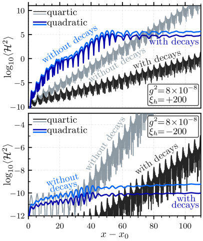
Figure 11: A comparison of the Higgs variance $\langle\mathcal{H}^{2}\rangle$ between massless and massive preheating, i.e., between the quartic and quadratic inflaton potentials, respectively, taking $m_{\phi}=10^{-5}$ and $\lambda_{\phi}=10^{-10}$. The backreaction effect is not included in this figure. The top and bottom panels show a difference in sign for the curvature coupling $\xi_{h}$. We have also included curves that show the result if perturbative decays are turned off. Notably, this effect is minimal in massive preheating but significant in the massless case. The contrast between the preheating scenarios is also evident in the short-lived growth of fluctuations for the massive case which ceases for $|q|\ll\frac{1}{4}$. Note that although $x$ and $\mathcal{H}$ have the same qualitative meaning in both preheating scenarios their explicit definitions differ due to the difference in background cosmology.

The logarithmic time-dependence of the decay exponent in Eq. (86) demonstrates a critical distinction between the massive and massless preheating scenarios. For the latter, the time-dependence of the decay exponent was found [in Eq. (55) and Eq. (56)] to be linear, making it possible for the perturbative decays to efficiently counter the growth of Higgs fluctuations, even shutting them down for sufficiently large quartic coupling. By contrast, the logarithmic time-dependence in massive preheating shows that the capacity for perturbative decays to stabilize the electroweak vacuum is relatively negligible. This distinction makes the features of the massless preheating dynamics somewhat unique.

In order to further illustrate this comparison, we have plotted the evolution of the Higgs variance $\langle\mathcal{H}^{2}\rangle$ in Fig. 11 for both the quadratic and quartic scenarios, using the quartic coupling $g^{2}/m_{\phi}^{2}=g^{2}/\lambda_{\phi}=800$ and curvature couplings $\xi_{h}=\pm 200$. The inflaton mass $m_{\phi}=10^{-5}$ and coupling $\lambda_{\phi}=10^{-10}$ are taken in the respective cases. In contrast to the unimpeded growth that arises from the quartic potential, we observe the end of particle production that occurs in the quadratic case once $|q|\lesssim 1/4$. And comparing the curves, which show the results with perturbative decays both included and not included, we see manifestly the relative importance of perturbative decays in these scenarios. Indeed, although the couplings are the same for each of the comparisons in Fig. 11, the results for vacuum stability can greatly differ. For instance, upon including backreaction one finds that, for the couplings in the bottom panel, the false vacuum survives in the quadratic case, but it decays in the quartic case. Notwithstanding, owing to the complex pattern of metastability regions for the quartic case, we can change this outcome with only a small change in the coupling.

An analytical study of the preheating dynamics and vacuum decay times is found in the literature for the unmixed case Ema et al. (2016), while the mixed case is studied mostly numerically in Ref. Ema et al. (2017). For the purpose of our comparison we shall focus on numerical results for $x_{\rm dec}$. Along these lines, we provide an analog to Fig. 10 for the massive preheating scenario in Fig. 12. Note that in order to make a clear comparison between this result and the massless preheating result in Fig. 10, we have constructed Fig. 12 using the same axes and axis scales. The gray exclusion regions correspond either to the Higgs destabilizing during inflation $\xi_{h}\lesssim-g^{2}\!/(2m_{\phi}^{2})$ or the flatness of the inflaton potential being ruined by quantum corrections $\xi_{h}\gtrsim\frac{1}{2}(10^{-6}-g^{2})/m_{\phi}^{2}$. The line showing $q=0$ is significant since along it the effective masses of the Higgs modes do not oscillate in time and the resonant particle production vanishes.

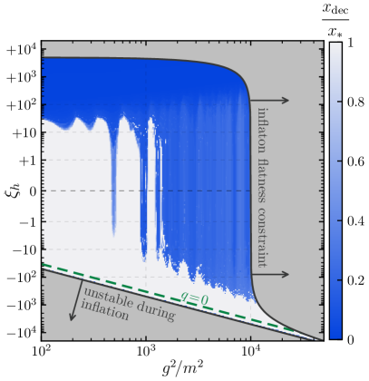
Figure 12: The decay time $x_{\rm dec}$ of the electroweak vacuum in the massive preheating scenario (for comparison with Fig. 10). The results are given relative to a fiducial time $x_{*}\approx 2\times 10^{3}$ for which the resonance is deep in the narrow regime over the parameter space shown. Our most immediate observation is that the metastable region is connected, which contrasts with the more complex disjoint regions found in the massless preheating scenario. The features appear consistent with the bounds found in previous studies in the literature Ema et al. (2016, 2017).

The most immediate observation we make in Fig. 12 is that the structure of the metastable region is relatively simple in comparison to Fig. 10. For $g^{2}/m_{\phi}^{2}\gtrsim 10^{3}$, the upper bound of the metastable region is roughly linear but flattens for smaller values of $g^{2}/m_{\phi}^{2}$. These results appear consistent with both Ref. Ema et al. (2016) and Ref. Ema et al. (2017). In particular, in Ref. Ema et al. (2016), bounds on the unmixed couplings were given approximately as $g^{2}/m^{2}\lesssim 10^{3}$ and $\xi\lesssim 10$, as reflected in our figure.

Appendix B Details for Tachyonic Production

In this appendix, we provide details of our calculations for which the non-minimal curvature couplings are dominant. Let us restate for convenience the general form given in Eq. (33) for the tachyonic growth in phase-space density $n_{h_{k}}$ for a given mode after passing through a tachyonic phase $j$ times Dufaux et al. (2006):

$$n_{h_{k}}~{}=~{}e^{2jX_{k}}\left(2\cos\Theta_{k}\right)^{2(j-1)}\ .$$ (87)

We recall that $X_{k}\equiv\int dt\,\Omega_{h_{k}}$ denotes the accumulated exponent when the effective mass of the mode is tachyonic and $\Theta_{k}\equiv\int dt\,\omega_{h_{k}}$ denotes the accumulated phase during the non-tachyonic intervals. Our primary objective is to evaluate these factors so that we may compute the variance of fluctuations $\langle h^{2}\rangle$ and, hence, the vacuum destabilization time for a given parameter set. In what follows, although the curvature terms have an overall time dependence, we neglect this within a single tachyonic interval.

Let us define functions $H_{1}(\alpha,\beta)$ and $H_{2}(\alpha,\beta)$ that will hold the oscillatory part of $X_{k}$ and $\Theta_{k}$. The way these functions are paired depends on the sign of the coupling. Namely, for the accumulated phase we have

$$\Theta_{k}=\begin{cases}2\sqrt{+r_{h}-\kappa^{2}}H_{1}(\alpha,\beta)&\text{for }\xi>0\\ 2\sqrt{-r_{h}+\kappa^{2}}H_{2}(\alpha,\beta)&\text{for }\xi<0\end{cases}\ ,$$ (88)

and for the growth exponent we have

$$X_{k}=\begin{cases}2\sqrt{+r_{h}-\kappa^{2}}H_{2}(\alpha,\beta)&\text{for }\xi>0\\ 2\sqrt{-r_{h}+\kappa^{2}}H_{1}(\alpha,\beta)&\text{for }\xi<0\end{cases}$$ (89)

and we have introduced the parameter combinations

$$\alpha~{}\equiv~{}\frac{3r_{h}}{r_{h}-\kappa^{2}}-2r_{\phi}\beta\ ,\qquad\ \beta~{}\equiv~{}\frac{g^{2}/\lambda_{\phi}}{r_{h}-\kappa^{2}}\ .$$ (90)

Meanwhile, the oscillatory functions are defined as

$$H_{1}(\alpha,\beta) \equiv\int_{0}^{x_{\times}}dx\sqrt{\beta\left(\frac{\varphi}{\overline{\varphi}}\right)^{\!\!2}+\alpha\left(\frac{\varphi}{\overline{\varphi}}\right)^{\!\!4}-1}$$

$$H_{2}(\alpha,\beta) \equiv\int_{x_{\times}}^{T\!/4}dx\sqrt{1-\beta\left(\frac{\varphi}{\overline{\varphi}}\right)^{\!\!2}-\alpha\left(\frac{\varphi}{\overline{\varphi}}\right)^{\!\!4}}$$ (91)

where $\varphi$ refers to the analytical solution for the background inflaton field in Eq. (16). Note that for our purposes here we take $x_{0}=0$. The quantity $x_{\times}$ is the crossing time that separates tachyonic and non-tachyonic phases of evolution for the mode, which can be expressed in terms of the inverse elliptic function as

$$x_{\times}(\alpha,\beta)~{}\equiv~{}\text{arccn}\!\left(\!\sqrt{\frac{\!-\beta+\sqrt{4\alpha+\beta^{2}}}{2\alpha}},\!\frac{1}{\sqrt{2}}\!\right)\ .$$ (92)

For the remainder of this appendix we shall focus solely on the accumulated exponent $X_{k}$ rather than the phase $\Theta_{k}$. While the latter is relevant for the detailed distribution of $n_{h_{k}}$, it is irrelevant to the overall growth. For clarity, we divide the following analysis in a manner parallel to Sec. III and Sec. IV in the paper, giving additional support to our derivation of results in the main text.

B.1 Pure Curvature Coupling ($g=0$)

In the limit of pure curvature coupling, our parameters in Eq. (90) reduce to $\alpha=3r_{h}/(r_{h}-\kappa^{2})$ and $\beta=0$, and the tachyonic phase appears only for $\alpha>1$. As in the main body of the paper, we ignore the $\xi<0$ region, since the vacuum is not stable. Identifying the limits $H_{1}(1,0)=0$ and $H_{2}(1,0)=\sqrt{2}$ along with

$$H_{1}(\alpha\rightarrow\infty,0)~{} \simeq~{}\frac{2\pi^{3/2}\sqrt{\alpha}}{\Gamma(\frac{1}{4})^{2}}$$

$$H_{2}(\alpha\rightarrow\infty,0)~{} \simeq~{}\sqrt{\frac{\pi}{2\sqrt{\alpha}}}\frac{\Gamma(\frac{5}{4})}{\Gamma(\frac{7}{4})}\ ,$$ (93)

we can construct the approximate fits

$$H_{1}(\alpha,0)~{} \simeq~{}\frac{2\pi^{3/2}\sqrt{\alpha-1}}{\Gamma(\frac{1}{4})^{2}}-\frac{0.59(\alpha-1)^{1/3}}{1+0.23\alpha}$$

$$H_{2}(\alpha,0)~{} \simeq~{}\sqrt{\frac{\pi}{2\sqrt{\alpha}}}\frac{\Gamma(\frac{5}{4})}{\Gamma(\frac{7}{4})}\left(1+\frac{\frac{2}{\sqrt{\pi}}\frac{\Gamma(7/4)}{\Gamma(5/4)}-1}{\alpha^{2}}\right)\ .$$ (94)

In the left panel in Fig. 13 we have plotted these fits (shown by solid curves) and the numerically integrated functions (shown by point markers) for comparison. By inspection of Eq. (90), we see that for $\xi>0$ we are confined to the range $\alpha\in[3,\infty)$. Likewise, for the $\xi<0$ region $\alpha\in(0,3]$ is required. The result in Eq. (34) for the tachyonic Higgs spectrum is then found directly using the leading terms in Eq. (94).

B.2 Mixed Case

As the mixed case with $\xi>0$ is fully addressed in Sec. III.3, let us address the $\xi<0$ region in this appendix, i.e., the derivation of the comoving number density Eq. (46). Note that given Eq. (90), this region corresponds to $\beta<0$. Additionally, the range of $\alpha$ is extended in the mixed-coupling case [according to Eq. (90)]. The dependence on both $\alpha$ and $\beta$ is important in what follows, so the fits above are not sufficient. But as we are interested in only the growth exponent $X_{k}$, we require only the $H_{1}(\alpha,\beta)$ function in this regime. This function has the approximate forms

$$H_{1}(\alpha,\beta)~{} \simeq~{}\frac{H_{1}(3,0)}{\sqrt{3}-1}\frac{\beta+\alpha-1}{\sqrt{\alpha}+1}$$

$$\simeq~{}\frac{H_{1}(3,0)}{2}\left(\beta+\alpha-1\right)\ .$$ (95)

While the first approximation gives a more accurate fit, the second is linear in both $\alpha$ and $\beta$ and useful for our estimates. We have plotted the latter approximation using solid curves in the right panel of Fig. 13, with point markers indicating the numerically integrated result.

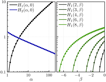
Figure 13: The functions $H_{1}(\alpha,\beta)$ and $H_{2}(\alpha,\beta)$ in Eq. (91) computed numerically (point markers) for comparison to our analytical approximations (shown by solid curves). The left panel shows the $\beta\rightarrow 0$ approximation for both functions from Eq. (94), and the right panel shows the approximation for $H_{1}(\alpha,\beta)$ derived in Eq. (95) for several values of $\alpha$.

Using this approximation, we find that the growth exponent is given up to $\mathcal{O}(\kappa^{2})$ by

$$2jX_{k}~{}\simeq~{}\frac{4H_{1}(3,0)}{T}\!\!\int\!dx\, \frac{\kappa^{2}-2r_{h}+\frac{g^{2}}{\lambda_{\phi}}\left(2r_{\phi}-1\right)}{\sqrt{\kappa^{2}-r_{h}}}\!$$ (96)

$$\simeq~{}\frac{-4H_{1}(3,0)}{T\sqrt{-6\xi}}\Bigg{\{}\!\Big{(}\xi_{\phi}\frac{g^{2}}{\lambda_{\phi}}+ \xi\Big{)}\Bigg{[}12\log\!\left(\frac{x}{x_{0}}\right)\!+\!\frac{\kappa^{2}(x^{2}\!-\!x_{0}^{2})}{2\xi}\Bigg{]}$$

$$\quad\ -\frac{1}{2}\!\Big{(}\frac{g^{2}}{\lambda_{\phi}}+ \kappa^{2}\Big{)}\!\Bigg{[}(x^{2}\!-x_{0}^{2})\!+\!\frac{\kappa^{2}(x^{4}\!-\!x_{0}^{4})}{24\xi}\Bigg{]}\Bigg{\}}$$

where $j$ is the number of times the effective Higgs mass has passed through the tachyonic region. Note that Eq. (46) is recovered in the $\kappa\rightarrow 0$ limit. The growth exponent readily gives the phase-space density $n_{h_{k}}$ via Eq. (87) if we neglect the oscillatory component $\Theta_{k}$.

Using the saddlepoint method to integrate over the momenta, we obtain the Higgs comoving number density

$$n_{h}\hskip 4.2679pt\simeq\hskip 4.2679pt \left(\!\!\frac{\sqrt{\lambda_{\phi}}\overline{\varphi}}{x}\!\right)^{\!\!\!3}\!\left[\!\frac{\frac{T}{4\pi H_{1}(3,0)}(-6\xi)^{3/2}}{-24\left(\xi_{\phi}\frac{g^{2}}{2\lambda_{\phi}}+\xi\right)-\frac{g^{2}}{2\lambda_{\phi}}x^{2}}\!\right]^{\!3/2}$$ (97)

$$\times\left(\frac{x}{x_{0}}\right)^{\!\!-\frac{8\sqrt{6}H_{1}(3,0)}{T\sqrt{-\xi}}\left(\xi_{\phi}\frac{g^{2}}{\lambda_{\phi}}+\xi\right)}e^{\frac{\sqrt{6}H_{1}(3,0)}{3T\sqrt{-\xi}}\frac{g^{2}}{\lambda_{\phi}}(x^{2}-x_{0}^{2})}\ ,$$

which is valid for times $x\lesssim x_{\xi}$. Using that the Higgs variance is $\langle h^{2}\rangle\simeq n_{h}/(a^{3}\omega_{h})$, we are finally in a position where we can produce the constraint in Eq. (75).

Appendix C Numerical Methods

In this appendix, we summarize the numerical methods used to compute the evolution of dynamical quantities in this paper. Note that analogous methods are applied for the comparison to massive preheating in Appendix A.

We perform our computations in the cosmological time $t$ and establish our initial conditions at the end of inflation. According to the analysis in Sec. II.1, the initial conditions at $t_{\rm end}$ are given by

$$\phi(t_{\rm end})~{} =~{}+\phi_{\rm end}$$

$$\dot{\phi}(t_{\rm end})~{} =~{}-\sqrt{V(\phi_{\rm end})}\ ,$$ (98)

where $\phi_{\rm end}=1$ is assumed. Furthermore, we assume for our numerics that the inflaton potential is given by a purely quartic potential $V(\phi)=\lambda_{\phi}\phi^{4}/4$, and we have neglected the difference between the canonical and non-canonical inflaton field. While this affects the initial velocity by an $\mathcal{O}(1)$ factor, we have checked that such changes have a negligible impact on our results.

The inflationary constraint in Eq. (11) is assumed so that the homogeneous value $h$ for the Higgs field is stabilized strongly at the origin. Even after the end of inflation, accounting for $h$ has a negligible influence on our results, so we ignore its equation of motion overall. We solve the equations of motion for the background inflaton field $\phi$, inflaton fluctuations $\phi_{k}$, and Higgs fluctuations $h_{k}$. As discussed in Sec. IV, the backreaction is accounted for using the Hartree approximation $h^{4}\rightarrow 6\langle h^{2}\rangle h^{2}-3\langle h^{2}\rangle^{2}$ for the Higgs self-interaction and using an analogous substitution for the quartic inflaton potential $\phi^{4}\rightarrow 6\langle\phi^{2}\rangle\phi^{2}-3\langle\phi^{2}\rangle^{2}$ Boyanovsky et al. (1995).

We discretize the momenta linearly over the range $k\in[0,\Lambda]$ with $N=300$ lattice points. The momentum cutoff $\Lambda$ is chosen based on the structure of the parametric and tachyonic instabilities; i.e., we use the maximal momentum of each unstable band. For example, with $\xi_{h}=0$ and $g^{2}/\lambda_{\phi}\gg 1$ our numerics use a cutoff near the maximum of the resonance band $\Lambda=\sqrt{\lambda_{\phi}}\overline{\varphi}(g^{2}/\lambda_{\phi})^{1/4}$.

The equations of motion are then given by

$$\ddot{\phi}+3H\dot{\phi}+\lambda_{\phi}\phi^{3}+3\lambda_{\phi}\langle\phi^{2}\rangle\phi+g^{2}\langle h^{2}\rangle\phi~{} =~{}0$$ (99)

$$\ddot{\phi}_{k}+3H\dot{\phi}_{k}+\omega_{\phi_{k}}^{2}\phi_{k}~{} =~{}0$$ (100)

$$\ddot{h}_{k}+(3H+\Gamma_{h_{k}})\dot{h}_{k}+\omega_{h_{k}}^{2}h_{k}~{} =~{}0\ ,$$ (101)

where the mode energies are

$$\omega_{\phi_{k}}^{2}~{} =~{}\frac{k^{2}}{a^{2}}+3\lambda_{\phi}\phi^{2}+3\lambda_{\phi}\langle\phi^{2}\rangle+g^{2}\langle h^{2}\rangle$$

$$\omega_{h_{k}}^{2}~{} =~{}\frac{k^{2}}{a^{2}}+g^{2}\phi^{2}+\xi_{h}R+g^{2}\langle\phi^{2}\rangle+3\lambda_{h}\langle h^{2}\rangle\ .$$ (102)

The Hubble parameter is computed using the first Friedmann equation $H^{2}=\rho_{\rm tot}/3$ for the total energy density $\rho_{\rm tot}$. Note that $\rho_{\rm tot}$ includes both the energy density of the inflaton background $\rho_{\phi}=\dot{\phi}^{2}/2+V(\phi)$ and that of the field fluctuations, although the latter do not provide a significant contribution until the system approaches the non-linear stage of preheating. We evolve these equations of motion until the Higgs destabilizes or the onset of non-linear dynamics is reached at $x_{\rm NL}\approx 400$.

The decay rates $\Gamma_{h_{k}}$ for the Higgs modes are calculated in the same way as Eq. (53), except in our numerical calculations we generally write $\Gamma_{h_{k}}=\Gamma_{h}/\gamma$, where the Lorentz factor $\gamma$ carries some momentum dependence.

The initial conditions for the field fluctuations in Eq. (100) and Eq. (101) are taken as Gaussian such that $\phi_{k}=1/\sqrt{2\omega_{\phi_{k}}}$ and $h_{k}=1/\sqrt{2\omega_{h_{k}}}$ at the initial time. However, this initial condition is UV divergent and sensitive to the cutoff scale $\Lambda$ introduced in our discretization. Employing adiabatic renormalization Postma and van de Vis (2017), we calculate the variance so that it is initially vanishing:

$$\langle h^{2}\rangle~{}\equiv~{}\frac{1}{2\pi^{2}}\int_{0}^{\Lambda}\!dk\,k^{2}\Big{[}\left|h_{k}(t)\right|^{2}-\frac{1}{a^{2}}\left|h_{k}(t_{\rm end})\right|^{2}\Big{]}\ .$$ (103)

The scaling of the counterterm with $a$ is chosen so that it scales with the physical momentum $k/a$.

Finally, we incorporate the running of the Higgs four-point coupling $\lambda_{h}(\mu)$ by evaluating the renormalization scale at $\smash{\mu=\sqrt{\langle h^{2}\rangle}}$. The effect of the backreaction is most relevant at energies near $h_{\rm SM}\approx 10^{10}\,\text{GeV}$ where, based on SM measurements, the coupling changes sign. Therefore, in our numerics we take the approximate

$$\lambda_{h}~{}=~{}0.01\,\text{sgn}\left(h_{\rm SM}-\sqrt{\langle h^{2}\rangle}\right)\ ,$$ (104)

which is similar to that used in other numerical studies Ema et al. (2016); Enqvist et al. (2016) of electroweak vacuum metastability.

References

- Zyla et al. (2020) P. A. Zyla et al. (Particle Data Group), PTEP 2020, 083C01 (2020).
- Degrassi et al. (2012) G. Degrassi, S. Di Vita, J. Elias-Miro, J. R. Espinosa, G. F. Giudice, G. Isidori, and A. Strumia, JHEP 08, 098 (2012), arXiv:1205.6497 [hep-ph] .
- Bezrukov et al. (2012) F. Bezrukov, M. Y. Kalmykov, B. A. Kniehl, and M. Shaposhnikov, JHEP 10, 140 (2012), arXiv:1205.2893 [hep-ph] .
- Alekhin et al. (2012) S. Alekhin, A. Djouadi, and S. Moch, Phys. Lett. B 716, 214 (2012), arXiv:1207.0980 [hep-ph] .
- Buttazzo et al. (2013) D. Buttazzo, G. Degrassi, P. P. Giardino, G. F. Giudice, F. Sala, A. Salvio, and A. Strumia, JHEP 12, 089 (2013), arXiv:1307.3536 [hep-ph] .
- Bednyakov et al. (2015) A. V. Bednyakov, B. A. Kniehl, A. F. Pikelner, and O. L. Veretin, Phys. Rev. Lett. 115, 201802 (2015), arXiv:1507.08833 [hep-ph] .
- Andreassen et al. (2018) A. Andreassen, W. Frost, and M. D. Schwartz, Phys. Rev. D 97, 056006 (2018), arXiv:1707.08124 [hep-ph] .
- Chigusa et al. (2018) S. Chigusa, T. Moroi, and Y. Shoji, Phys. Rev. D 97, 116012 (2018), arXiv:1803.03902 [hep-ph] .
- Markkanen et al. (2018) T. Markkanen, A. Rajantie, and S. Stopyra, Front. Astron. Space Sci. 5, 40 (2018), arXiv:1809.06923 [astro-ph.CO] .
- East et al. (2017) W. E. East, J. Kearney, B. Shakya, H. Yoo, and K. M. Zurek, Phys. Rev. D 95, 023526 (2017), arXiv:1607.00381 [hep-ph] .
- Fumagalli et al. (2020) J. Fumagalli, S. Renaux-Petel, and J. W. Ronayne, JHEP 02, 142 (2020), arXiv:1910.13430 [hep-ph] .
- Espinosa et al. (2008) J. R. Espinosa, G. F. Giudice, and A. Riotto, JCAP 05, 002 (2008), arXiv:0710.2484 [hep-ph] .
- Lebedev and Westphal (2013) O. Lebedev and A. Westphal, Phys. Lett. B 719, 415 (2013), arXiv:1210.6987 [hep-ph] .
- Felder et al. (2001a) G. N. Felder, J. Garcia-Bellido, P. B. Greene, L. Kofman, A. D. Linde, and I. Tkachev, Phys. Rev. Lett. 87, 011601 (2001a), arXiv:hep-ph/0012142 .
- Felder et al. (2001b) G. N. Felder, L. Kofman, and A. D. Linde, Phys. Rev. D 64, 123517 (2001b), arXiv:hep-th/0106179 .
- Dufaux et al. (2006) J. F. Dufaux, G. N. Felder, L. Kofman, M. Peloso, and D. Podolsky, JCAP 07, 006 (2006), arXiv:hep-ph/0602144 .
- Kofman et al. (1994) L. Kofman, A. D. Linde, and A. A. Starobinsky, Phys. Rev. Lett. 73, 3195 (1994), arXiv:hep-th/9405187 .
- Kofman et al. (1997) L. Kofman, A. D. Linde, and A. A. Starobinsky, Phys. Rev. D 56, 3258 (1997), arXiv:hep-ph/9704452 .
- Greene et al. (1997) P. B. Greene, L. Kofman, A. D. Linde, and A. A. Starobinsky, Phys. Rev. D 56, 6175 (1997), arXiv:hep-ph/9705347 .
- Herranen et al. (2015) M. Herranen, T. Markkanen, S. Nurmi, and A. Rajantie, Phys. Rev. Lett. 115, 241301 (2015), arXiv:1506.04065 [hep-ph] .
- Ema et al. (2016) Y. Ema, K. Mukaida, and K. Nakayama, JCAP 10, 043 (2016), arXiv:1602.00483 [hep-ph] .
- Kohri and Matsui (2016) K. Kohri and H. Matsui, Phys. Rev. D 94, 103509 (2016), arXiv:1602.02100 [hep-ph] .
- Enqvist et al. (2016) K. Enqvist, M. Karciauskas, O. Lebedev, S. Rusak, and M. Zatta, JCAP 11, 025 (2016), arXiv:1608.08848 [hep-ph] .
- Ema et al. (2017) Y. Ema, M. Karciauskas, O. Lebedev, and M. Zatta, JCAP 06, 054 (2017), arXiv:1703.04681 [hep-ph] .
- Gross et al. (2016) C. Gross, O. Lebedev, and M. Zatta, Phys. Lett. B 753, 178 (2016), arXiv:1506.05106 [hep-ph] .
- Kasuya and Kawasaki (1996) S. Kasuya and M. Kawasaki, Phys. Lett. B 388, 686 (1996), arXiv:hep-ph/9603317 .
- Felder et al. (1999) G. N. Felder, L. Kofman, and A. D. Linde, Phys. Rev. D 59, 123523 (1999), arXiv:hep-ph/9812289 .
- Bezrukov et al. (2009) F. Bezrukov, D. Gorbunov, and M. Shaposhnikov, JCAP 06, 029 (2009), arXiv:0812.3622 [hep-ph] .
- Garcia-Bellido et al. (2009) J. Garcia-Bellido, D. G. Figueroa, and J. Rubio, Phys. Rev. D 79, 063531 (2009), arXiv:0812.4624 [hep-ph] .
- Mukaida and Nakayama (2013) K. Mukaida and K. Nakayama, JCAP 03, 002 (2013), arXiv:1212.4985 [hep-ph] .
- Repond and Rubio (2016) J. Repond and J. Rubio, JCAP 07, 043 (2016), arXiv:1604.08238 [astro-ph.CO] .
- Fan et al. (2021) J. Fan, K. D. Lozanov, and Q. Lu, JHEP 05, 069 (2021), arXiv:2101.11008 [hep-ph] .
- Buchbinder et al. (1992) I. L. Buchbinder, S. D. Odintsov, and I. L. Shapiro, Effective action in quantum gravity (1992).
- Akrami et al. (2020) Y. Akrami et al. (Planck), Astron. Astrophys. 641, A10 (2020), arXiv:1807.06211 [astro-ph.CO] .
- Spokoiny (1984) B. L. Spokoiny, Phys. Lett. B 147, 39 (1984).
- Futamase and Maeda (1989) T. Futamase and K.-i. Maeda, Phys. Rev. D 39, 399 (1989).
- Salopek et al. (1989) D. S. Salopek, J. R. Bond, and J. M. Bardeen, Phys. Rev. D 40, 1753 (1989).
- Fakir and Unruh (1990) R. Fakir and W. G. Unruh, Phys. Rev. D 41, 1783 (1990).
- Bezrukov and Shaposhnikov (2008) F. L. Bezrukov and M. Shaposhnikov, Phys. Lett. B 659, 703 (2008), arXiv:0710.3755 [hep-th] .
- Salvio and Strumia (2014) A. Salvio and A. Strumia, JHEP 06, 080 (2014), arXiv:1403.4226 [hep-ph] .
- Csaki et al. (2014) C. Csaki, N. Kaloper, J. Serra, and J. Terning, Phys. Rev. Lett. 113, 161302 (2014), arXiv:1406.5192 [hep-th] .
- Kannike et al. (2015) K. Kannike, G. Hütsi, L. Pizza, A. Racioppi, M. Raidal, A. Salvio, and A. Strumia, JHEP 05, 065 (2015), arXiv:1502.01334 [astro-ph.CO] .
- Palatini (1919) A. Palatini, Rendiconti del Circolo Matematico di Palermo (1884-1940) 43, 203 (1919).
- Einstein (1925) A. Einstein, Sitzungsber. K. Preuss. Akad. Wiss. 43, 414 (1925).
- Bauer and Demir (2008) F. Bauer and D. A. Demir, Phys. Lett. B 665, 222 (2008), arXiv:0803.2664 [hep-ph] .
- Misner et al. (1973) C. W. Misner, K. S. Thorne, and J. A. Wheeler, Gravitation (W. H. Freeman, San Francisco, 1973).
- Dufaux et al. (2010) J.-F. Dufaux, D. G. Figueroa, and J. Garcia-Bellido, Phys. Rev. D 82, 083518 (2010), arXiv:1006.0217 [astro-ph.CO] .
- Karamitsos and Pilaftsis (2018) S. Karamitsos and A. Pilaftsis, Nucl. Phys. B 927, 219 (2018), arXiv:1706.07011 [hep-ph] .
- Kallosh et al. (2013) R. Kallosh, A. Linde, and D. Roest, JHEP 11, 198 (2013), arXiv:1311.0472 [hep-th] .
- Galante et al. (2015) M. Galante, R. Kallosh, A. Linde, and D. Roest, Phys. Rev. Lett. 114, 141302 (2015), arXiv:1412.3797 [hep-th] .
- Carrasco et al. (2015) J. J. M. Carrasco, R. Kallosh, and A. Linde, JHEP 10, 147 (2015), arXiv:1506.01708 [hep-th] .
- Renaux-Petel and Turzyński (2016) S. Renaux-Petel and K. Turzyński, Phys. Rev. Lett. 117, 141301 (2016), arXiv:1510.01281 [astro-ph.CO] .
- Bond et al. (2009) J. R. Bond, A. V. Frolov, Z. Huang, and L. Kofman, Phys. Rev. Lett. 103, 071301 (2009), arXiv:0903.3407 [astro-ph.CO] .
- Rusak (2020) S. Rusak, JCAP 05, 020 (2020), arXiv:1811.10569 [hep-ph] .
- Fu et al. (2017) C. Fu, P. Wu, and H. Yu, Phys. Rev. D 96, 103542 (2017), arXiv:1801.04089 [gr-qc] .
- Karam et al. (2021) A. Karam, M. Raidal, and E. Tomberg, JCAP 03, 064 (2021), arXiv:2007.03484 [astro-ph.CO] .
- Turner (1983) M. S. Turner, Phys. Rev. D 28, 1243 (1983).
- Whittaker and Watson (1996) E. T. Whittaker and G. N. Watson, A Course of Modern Analysis, 4th ed., Cambridge Mathematical Library (Cambridge University Press, 1996).
- Lachapelle and Brandenberger (2009) J. Lachapelle and R. H. Brandenberger, JCAP 04, 020 (2009), arXiv:0808.0936 [hep-th] .
- Choi et al. (2019) S.-M. Choi, Y.-J. Kang, H. M. Lee, and K. Yamashita, JHEP 05, 060 (2019), arXiv:1902.03781 [hep-ph] .
- Lebedev and Yoon (2021) O. Lebedev and J.-H. Yoon, (2021), arXiv:2105.05860 [hep-ph] .
- Boyanovsky et al. (1995) D. Boyanovsky, H. J. de Vega, R. Holman, D. S. Lee, and A. Singh, Phys. Rev. D 51, 4419 (1995), arXiv:hep-ph/9408214 .
- Khlebnikov and Tkachev (1996) S. Y. Khlebnikov and I. I. Tkachev, Phys. Rev. Lett. 77, 219 (1996), arXiv:hep-ph/9603378 .
- Fukugita and Yanagida (1986) M. Fukugita and T. Yanagida, Phys. Lett. B 174, 45 (1986).
- Almeida et al. (2019) J. P. B. Almeida, N. Bernal, J. Rubio, and T. Tenkanen, JCAP 03, 012 (2019), arXiv:1811.09640 [hep-ph] .
- Babichev et al. (2020) E. Babichev, D. Gorbunov, S. Ramazanov, and L. Reverberi, JCAP 09, 059 (2020), arXiv:2006.02225 [hep-ph] .
- Harigaya and Mukaida (2014) K. Harigaya and K. Mukaida, JHEP 05, 006 (2014), arXiv:1312.3097 [hep-ph] .
- Mukaida and Yamada (2016) K. Mukaida and M. Yamada, JCAP 02, 003 (2016), arXiv:1506.07661 [hep-ph] .
- Delle Rose et al. (2016) L. Delle Rose, C. Marzo, and A. Urbano, JHEP 05, 050 (2016), arXiv:1507.06912 [hep-ph] .
- Chambers and Rajantie (2008) A. Chambers and A. Rajantie, JCAP 08, 002 (2008), arXiv:0805.4795 [astro-ph] .
- Garcia et al. (2020) M. A. G. Garcia, K. Kaneta, Y. Mambrini, and K. A. Olive, Phys. Rev. D 101, 123507 (2020), arXiv:2004.08404 [hep-ph] .
- Garcia et al. (2021) M. A. G. Garcia, K. Kaneta, Y. Mambrini, and K. A. Olive, JCAP 04, 012 (2021), arXiv:2012.10756 [hep-ph] .
- Cline et al. (2020) J. M. Cline, M. Puel, and T. Toma, Phys. Rev. D 101, 043014 (2020), arXiv:1909.12300 [hep-ph] .
- Kawasaki and Ueda (2021) M. Kawasaki and S. Ueda, JCAP 04, 049 (2021), arXiv:2011.10397 [hep-ph] .
- (75) J. Kost, C. S. Shin, and T. Terada, in preparation.
- Linde (1994) A. D. Linde, Phys. Rev. D 49, 748 (1994), arXiv:astro-ph/9307002 .
- Garcia-Bellido and Linde (1998) J. Garcia-Bellido and A. D. Linde, Phys. Rev. D 57, 6075 (1998), arXiv:hep-ph/9711360 .
- Shaposhnikov et al. (2021a) M. Shaposhnikov, A. Shkerin, I. Timiryasov, and S. Zell, JCAP 02, 008 (2021a), arXiv:2007.14978 [hep-ph] .
- Shaposhnikov et al. (2020) M. Shaposhnikov, A. Shkerin, I. Timiryasov, and S. Zell, JHEP 10, 177 (2020), arXiv:2007.16158 [hep-th] .
- Shaposhnikov et al. (2021b) M. Shaposhnikov, A. Shkerin, I. Timiryasov, and S. Zell, Phys. Rev. Lett. 126, 161301 (2021b), [Erratum: Phys.Rev.Lett. 127, 169901 (2021)], arXiv:2008.11686 [hep-ph] .
- Figueroa and Torrenti (2017) D. G. Figueroa and F. Torrenti, JCAP 10, 057 (2017), arXiv:1707.04533 [astro-ph.CO] .
- Aggarwal et al. (2020) N. Aggarwal et al., (2020), arXiv:2011.12414 [gr-qc] .
- Domcke and Garcia-Cely (2021) V. Domcke and C. Garcia-Cely, Phys. Rev. Lett. 126, 021104 (2021), arXiv:2006.01161 [astro-ph.CO] .
- Cai et al. (2022) R.-G. Cai, Z.-K. Guo, P.-Z. Ding, C.-J. Fu, and J. Liu, Phys. Rev. D 105, 023507 (2022), arXiv:2105.00427 [astro-ph.CO] .
- Postma and van de Vis (2017) M. Postma and J. van de Vis, JCAP 05, 004 (2017), arXiv:1702.07636 [hep-ph] .