Holographic phonons by gauge-axion coupling

Abstract

In this paper, we show that a simple generalization of the holographic axion model can realize spontaneous breaking of translational symmetry by considering a special gauge-axion higher derivative term. The finite real part and imaginary part of the stress tensor imply that the dual boundary system is a viscoelastic solid. By calculating quasi-normal modes and making a comparison with predictions from the elasticity theory, we verify the existence of phonons and pseudo-phonons, where the latter is realized by introducing a weak explicit breaking of translational symmetry, in the transverse channel. Finally, we discuss how the phonon dynamics affects the charge transport.

I Introduction

It is widely unveiled that the hydrodynamic formulation, which is based upon a small amount of conserved quantities as well as the constitutive relations, can provide a universal description for the low energy collective excitations in exotic quantum matter Teaney (2010); O’Hara et al. (2002); Levitov and Falkovich (2016); Bandurin and et al (2016). In relativistic hydrodynamics Kovtun (2012), the most fundamental conserved quantity is the stress tensor. Despite the Poincaré symmetry is fundamental for particles in the high energy region, the spatial translations are ubiquitously broken at low energy scales in condensed matter physics, especially in solids where there commonly exist periodic lattice, impurities, defects, etc. If the breaking of translations is weak, we are still allowed to formulate the so-called quasi-hydrodynamics to address the problems approximately. However, this framework might break down when the translational symmetry is strongly violated.

On the contrary, the holographic duality provides a purely geometric approach to understand universal behaviors in strongly coupled systems, regardless of whether quantities are conserved or not Hartnoll (2009); Natsuume (2015); McGreevy ; Hartnoll et al. (2016a). In holography, all the physics of a many-body system (which is described by some quantum field theories) is encoded in a dual gravity theory with one extra dimension. Moreover, in the strong coupling limit of the field theory, the quantum effects on the gravity side are significantly suppressed. As a result, complicated problems on the field theory side are simplified into solving classical equations in a curved spacetime. Consequently, this duality has nowadays become a widely used tool for exploring strongly coupled many-body systems.

Despite the earlier holographic studies focused more on translation invariant systems, some recent work attempts to make setups closer to realistic materials without translations Horowitz et al. (2012a, b); Donos and Hartnoll (2013); Vegh (2013); Horowitz and Santos (2013); Blake and Tong (2013); Ling et al. (2013); Donos and Gauntlett (2014a); Andrade and Withers (2014); Donos and Gauntlett (2014b); Goutéraux (2014); Ling et al. (2015); Davison and Goutéraux (2015a); Donos and Pantelidou (2019). One of the simplest ways to capture the key features of the symmetry breaking patterns of translations but allow fast calculations is to consider homogeneous massive gravity models. Based on the perturbative calculations, it has also been explicitly shown that gravitons always have a non-zero mass in any holographic system with an inhomogeneous lattice Blake et al. (2014). For this reason, massive gravity provides a universal low energy description for strongly coupled systems with broken translations. A generally and widely used way of modeling massive gravity is to consider the axions in the bulk Baggioli and Pujolas (2015); Alberte and Khmelnitsky (2015); Alberte et al. (2016a); Baggioli and Pujolas (2016); Alberte et al. (2018a). These are massless scalars enjoying a internal shift symmetry, linearly depending on spatial coordinates. As a result, the background configuration of the axions contributes a non-zero mass to gravitons, breaking the translations in the boundary system but retaining the homogeneity of the background. Better yet, one can easily realize explicit breaking (ESB) or spontaneous breaking (SSB) of translations differently by slightly changing the kinetic term of the axions in the bulk Alberte et al. (2018b); Ammon et al. (2019a, b); Baggioli and Grieninger (2019) . For a comprehensive review on the holographic axion models, one refers to Baggioli et al. (2021).

In this work, we consider a new way of spontaneously breaking translations by directly coupling the axions to the $U(1)$ gauge field at finite density. Note that such types of gauge-axion higher derivative terms have previously introduced in Goutéraux et al. (2016); Baggioli et al. (2017) in the holographic studies on the metal-insulator transition (MIT). Here, we consider the simplest one of them and reveal the fact that this term just introduces a spontaneous breaking of translations and the pinning effect in presence of external sources leads to the MIT. Moreover, different from the fluid model discussed in Li and Wu (2019), the gravity system under consideration is dual to some solid states on boundary where there exist propagating/pinned modes in the transverse channel. The paper is organized as follows: In Section II, we introduce the holographic setup, solve the background solution and analyze the viscoelasticity of the dual system. In Section III, the spectrum of transverse phonons is systematically investigated by computing quasi-normal modes (QNMs) of the black hole. In Section IV, we study how the phononic dynamics impacts the charge transport. In Section V, we conclude.

II An elastic black hole

II.1 Spontaneous breaking of translations

In this paper, we consider the following action which can break translational symmetry of dual field theories (Goutéraux et al., 2016)

$$S=\int d^{4}x\sqrt{-g}\left[R-2\Lambda-\lambda X-\frac{1}{4}\left(1+\mathcal{K}X\right)F^{2}\right],$$ (1)

where $X$ is the kinetic term of the axions $\phi^{I}$ and $F_{\mu\nu}$ is $U(1)$ gauge field which are described by

$$X=\frac{1}{2}\sum_{I=x,y}\partial^{\mu}\phi^{I}\partial_{\mu}\phi^{I},\qquad F_{\mu\nu}=\nabla_{\mu}A_{\nu}-\nabla_{\nu}A_{\mu}.$$ (2)

And, $\Lambda$ is the cosmological constant that will be set $\Lambda=-3$ for simplicity. $\lambda$ and $\mathcal{K}$ are dimensionless couplings. If we set $\mathcal{K}=0$, this action simply reduces to the simple linear axion model Andrade and Withers (2014). In our model, we should require that $\lambda\geq 0$ for avoiding the ghost problem and $-1/6\leq\mathcal{K}\leq 0$ for causality and stability Baggioli and Pujolas (2017); Goutéraux et al. (2016) .

Varying the bulk fields, their equations of motion are given by

$$R_{\mu\nu}-\frac{1}{2}g_{\mu\nu}R-\frac{1}{2}(\lambda+\frac{\mathcal{K}}{4}F_{\sigma\rho}F^{\sigma\rho})\nabla_{\mu}\phi^{I}\nabla_{\nu}\phi^{I}-\frac{1}{2}\left(6-\frac{\lambda}{2}\nabla_{\sigma}\phi^{I}\nabla^{\sigma}\phi^{I}\right)g_{\mu\nu}$$ (3)

$$=\frac{1}{2}\left(1+\frac{\mathcal{K}}{2}\nabla_{\sigma}\phi^{I}\nabla^{\sigma}\phi^{I}\right)\Big{(}{F_{\mu}}^{\sigma}F_{\nu\sigma}-\frac{1}{4}g_{\mu\nu}F_{\rho\sigma}F^{\rho\sigma}\Big{)},$$

$$\nabla_{\mu}\left[\left(1+\frac{\mathcal{K}}{2}\nabla_{\sigma}\phi^{I}\nabla^{\sigma}\phi^{I}\right)F^{\mu\nu}\right]=0,$$ (4)

and

$$\nabla_{\mu}\Big{[}\lambda\nabla^{\mu}\phi^{I}-\frac{1}{4}\left(\mathcal{K}(\nabla^{\mu}\phi^{I})F^{2}\right)\Big{]}=0.$$ (5)

Note that in holographic axion models, we have the following isotropic and homogeneous background metric,

$$ds^{2}=\frac{1}{u^{2}}\left[-f(u)dt^{2}+\frac{1}{f(u)}du^{2}+dx^{2}+dy^{2}\right],$$ (6)

$$A=A_{t}(u)dt,\qquad\phi^{I}=\alpha\delta^{I}_{i}x^{i},$$ (7)

where $\alpha$ is a constant characterizing the breaking of translations, and $x^{i}$ denotes the boundary spatial coordinates. AdS boundary is located at $u=0$ and horizon is determined by $f(u=u_{h})=0$ in this convention. For our model, we can solve the black hole solution analytically

$$f(u)=1-\frac{1}{2}\alpha^{2}\lambda u^{2}+\frac{\rho^{2}u^{3}ArcTanh\left(\alpha\sqrt{-\mathcal{K}}u\right)}{4\alpha\sqrt{-\mathcal{K}}}-\frac{\rho^{2}u^{3}ArcTanh\left(\alpha\sqrt{-\mathcal{K}}u_{h}\right)}{4\alpha\sqrt{-\mathcal{K}}}-\frac{u^{3}}{u_{h}^{3}}+\frac{\alpha^{2}\lambda u^{3}}{2u_{h}},$$ (8)

$$A_{t}(u)=\mu-\frac{\rho ArcTanh\left(\alpha\sqrt{-\mathcal{K}}u\right)}{\alpha\sqrt{-\mathcal{K}}}.$$ (9)

Here, $\mu$ and $\rho$ are two integration constants which are interpreted as chemical potential and charge density in the dual field theory. The regularity for gauge field $A_{\mu}$ on the horizon requires

$$\mu=\frac{\rho ArcTanh\left(\alpha\sqrt{-\mathcal{K}}u_{h}\right)}{\alpha\sqrt{-\mathcal{K}}}.$$ (10)

According to the holographic dictionary, entropy density, energy density, momentum susceptibility and temperature are respectively given by

$$s=\frac{4\pi}{u_{h}^{2}},\qquad\epsilon=2\left(\frac{1}{u_{h}^{3}}-\frac{\lambda\alpha^{2}}{2u_{h}}+\frac{\rho^{2}ArcTanh\left(\alpha\sqrt{-\mathcal{K}}u_{h}\right)}{4\alpha\sqrt{-\mathcal{K}}}\right),$$ (11)

$$\chi_{PP}=\epsilon+P=\frac{3}{2}\epsilon,\qquad T=\frac{3}{4\pi u_{h}}-\frac{\lambda\alpha^{2}u_{h}}{8\pi}-\frac{\rho^{2}u_{h}^{3}}{16\pi(1+\mathcal{K}\alpha^{2}u_{h}^{2})},$$ (12)

where $\chi_{PP}=\epsilon+P=3/2\epsilon$ comes from conformal invariance.

Next, we will explain the two different manners of breaking translations by analyzing the asymptotic behavior of scalar field $\phi^{I}$ close to the AdS boundary $(u\rightarrow 0)$. The story is very similar as in Amoretti et al. (2017); Alberte et al. (2018b); Amoretti et al. (2018a, b); Li and Wu (2019); Amoretti et al. (2019a).

• If we set $\lambda\neq 0$ and $\mathcal{K}=0$ in (5), the asymptotic expansion of $\phi^{I}$ near the UV boundary is

  $$\phi^{I}=\phi_{(0)}^{I}(t,x^{i})+\phi_{(3)}^{I}(t,x^{i})u^{3}+\cdots.$$ (13)

  According to the holographic dictionary and standard quantization, the leading order $\phi_{(0)}^{I}(t,x^{i})=\alpha x^{I}\neq 0$ plays the role of external source that breaks translations explicitly, relaxing the momentum on the field theory side. Further properties and applications in holography have been widely investigated in Andrade and Withers (2014); Davison and Goutéraux (2015a); Kim et al. (2014, 2015); Davison and Goutéraux (2015b); Blake et al. (2018); Zhou et al. (2020).

• If we instead set $\lambda=0$ and $\mathcal{K}\neq 0$, the asymptotic expansion of scalar field will be changed by

  $$\phi^{I}=\frac{\phi_{(-1)}^{I}(t,x^{i})}{u}+\phi_{(0)}^{I}(t,x^{i})+\cdots.$$ (14)

  In this case, the background solution of $\phi^{I}$ means that the leading $\phi_{(-1)}^{I}(t,x^{i})$-term associated to the source should be turned off while existing a non-zero expectation value $<\mathcal{O}^{I}>$ $\sim$ $\phi_{(0)}^{I}(t,x^{i})=\alpha x^{I}$. This implies the pattern of spontaneous breaking of translational symmetry.

Note that if the translations are broken spontaneously, there should exist gapless excitations in the low energy description which are called Goldstone modes. In solid state physics, these Goldstone modes are called phonons, the propagating sound modes in elastic media. The dynamics of Goldstone modes has already been studied in holography Alberte et al. (2018b); Ammon et al. (2019a, b); Baggioli and Grieninger (2019); Amoretti et al. (2019a); Donos et al. (2020); Amoretti et al. (2020a); Baggioli et al. (2020a) and field theory Leutwyler (1997); Dubovsky et al. (2006); Nicolis et al. (2015); Delacrétaz et al. (2017); Alberte et al. (2019); Musso (2019).

II.2 Shear viscoelasticity

One of the most distinctions of a solid and a fluid is that the former is resistant to shear deformations while the latter one is not. To show that the black hole solution under consideration is dual to a solid system, we shall compute the Green function of the stress tensor, which in the hydrodynamic regime can be expressed as

$$\mathcal{G}^{R}_{T_{xy}T_{xy}}(\omega,k=0)=G\,-i\,\omega\,\eta+\cdots,$$ (15)

where $G$ is the shear elastic modulus and $\eta$ is the shear viscosity. In the rest of this subsection, we focus on the purely SSB pattern by turning off the external source, i.e, setting $\lambda=0$ and remaining $\mathcal{K}\neq 0$. One can calculate $G$ and $\eta$ via retarded Green functions of stress tensor operator $T_{xy}$ numerically and read them by Ammon et al. (2019a)

$$G=Re\left[\mathcal{G}_{T_{xy}T_{xy}}^{R}(\omega=k=0)\right],\qquad\eta=-\lim_{\omega\rightarrow 0}\frac{1}{\omega}Im\left[\mathcal{G}_{T_{xy}T_{xy}}^{R}(\omega,k=0)\right].$$ (16)

The numeric results have been shown in Fig.1. And we find that the ratio of shear viscosity $\eta$ to entropy density $s$ always breaks Kovtun-Son-Starinets (KSS) bound Kovtun et al. (2005) due to the breaking of translations. Moreover, there is a non-trivial shear modulus which implies the dual system is in a solid state. To have it positive, i.e avoiding dynamical instability, we should always require that $\mathcal{K}<0$ in our model.

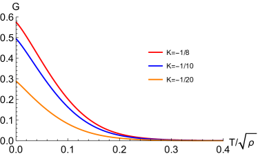
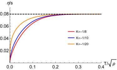
Figure 1: The dependence of the shear elastic modulus $G$ and the ratio of $\eta/s$ on $T/\sqrt{\rho}$ for different $\mathcal{K}$. The black dashed line is KSS bound $1/4\pi$ Kovtun et al. (2005). We have fixed coupling $\lambda=0$.

Now, we analyze the Green function $\mathcal{G}_{T_{xy}T_{xy}}^{R}$ analytically in the high and low temperature limits. Let us focus on the former first. The details of the calculation are shown in the Appendix A. In the high temperature limit, the analytical results of shear modulus and viscosity are respectively given by

$$G=-\frac{9\mathcal{K}\alpha^{2}T}{128\pi^{3}}\left(\frac{\sqrt{\rho}}{T}\right)^{4}+\cdots,$$ (17)

$$\frac{\eta}{s}=\frac{1}{4\pi}+\frac{81\mathcal{K}\alpha^{2}}{16384\pi^{7}T^{2}}\left(\frac{\sqrt{\rho}}{T}\right)^{4}+\cdots.$$ (18)

Note that the positive shear modulus again requires the coupling constant $\mathcal{K}<0$.

In the low temperature limit, we only find the analytical result for $\eta$ that is given by

$$\frac{\eta}{s}\sim\left(\frac{T}{\sqrt{\rho}}\right)^{2\xi-1},\qquad\xi=\frac{1}{2}\sqrt{1-\frac{8\sqrt{3}\mathcal{K}}{\sqrt{3\mathcal{K}^{2}+1}}}.$$ (19)

This result is slightly different from the massive gravity without charge density Baggioli (2019), which shows that the ratio is proportional to $T^{2}$. The author of Hartnoll et al. (2016b) have claimed that $T^{2}$ was the fastest decay for the models whose IR geometry has an $AdS_{2}$ factor. In our case, the maximum of exponent is $T^{2}$ that is corresponding to $\mathcal{K}\rightarrow-\infty$, which satisfies this bound. However, this claim is not true anymore if one consider more complicated IR fixed points (see Ling et al. (2016)). Note that for $\mathcal{K}=0$ the $\eta/s$ ratio is a constant which should be KSS bound.

III Holographic transverse phonons

III.1 Gapless phonons

The dispersion relation of transverse phonons at low energy is

$$\omega=\pm c_{T}k-iD_{T}k^{2}+\cdots,$$ (20)

where $c_{T}$ is the propagation velocity of phonons, which is related to the shear elastic modulus of material given by

$$c_{T}^{2}=\frac{G}{\chi_{PP}}.$$ (21)

$D_{T}$ is the attenuation constant that is related to the shear viscosity $\eta$ by $D_{T}=\eta/\chi_{PP}$ Amoretti et al. (2019a). In order to confirm the presence of transverse phonons, we compute the quasi-normal modes (QNMs) numerically at zero and finite momenta in the infalling Eddington-Finkelstein coordinates (74) by using the pseudo-spectral method. It shows that the Goldstone modes induced by SSB of translations can be confirmed as transverse phonons in this holographic model (1). One can see more numerical details in Jansen (2017).

In Fig.2, we show the real and imaginary parts of the lowest order QNMs for different temperatures. These Goldstone modes are phonons we expected. The spectrums of QNMs for different couplings are shown in Fig.3. One can calculate the sound speed of the transverse phonons in terms of (21) by holography and compare them to the numeric results extracted from QNMs. We find that they are in perfect agreement with each other, as is shown in Fig.4.

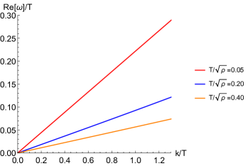
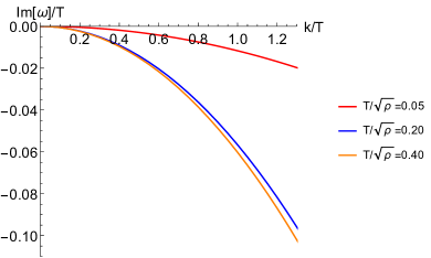
Figure 2: Real and imaginary parts of the lowest QNMs for different temperatures. We have fixed coupling $\mathcal{K}=-1/8$ and $\lambda=0$. We try to use the generalized dispersion relation $\omega=c_{1}k^{a}+ic_{2}k^{b}$ to fit the QNMs data. In our numerical cases, we get $a=1.00003\pm 0.00002$ and $b=2.00003\pm 0.00003$, which satisfies the dispersion relation (20).

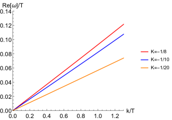
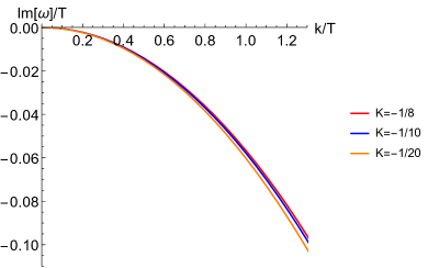
Figure 3: Real and imaginary parts of the lowest QNMs for different couplings $\mathcal{K}$. We have fixed $T/\sqrt{\rho}=0.2$ and $\lambda=0$.

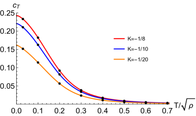
Figure 4: Comparison of the sound velocity extracted from QNMs (black dots) and the result from the elasticity formula (21) (solid lines) for various values of $\mathcal{K}$.

III.2 Pinned phonons

In this section, we further introduce slow relaxation on momentum into the SSB pattern. Physically, this makes the momentum operator no longer exactly conserved and the would be massless Goldstones get slightly gapped (which is now called pseudo-Goldstones or pinned phonons). In our model it can be easily realized by including the canonical kinetic term of the axions as follows,

$$\mathcal{L}_{\phi} =-\lambda X-\frac{1}{4}\mathcal{K}XF^{2}.$$ (22)

In order not to change the SSB pattern significantly, we assume that the value of $\lambda$ is small comparing to $\mathcal{K}$.

In presence of slow momentum relaxation, the relaxation rate $\Gamma$ is controlled in the manner of Andrade and Withers (2014); Davison (2013)

$$\Gamma\propto\lambda\,\alpha^{2}.$$ (23)

Therefore we can define a ESB scale which depicts the strength of explicit breaking of symmetry

$$\langle\textsl{ESB}\rangle\equiv\sqrt{\lambda}\,\alpha.$$ (24)

Heuristically, we define the SSB scale as follows

$$\langle\textsl{SSB}\rangle\equiv\sqrt{\frac{-\mathcal{K}}{4}}\,\alpha.$$ (25)

Then, the competition of SSB and ESB should be described by a dimensionless parameter that is defined by

$$\beta\equiv\frac{\langle\textsl{SSB}\rangle}{\langle\textsl{ESB}\rangle}=\sqrt{\frac{-\mathcal{K}}{4\,\lambda}}.$$ (26)

That is to say that at $\beta=0$ the breaking of translations is totally explicit while at $\beta=\infty$ purely spontaneous. Then, the pinned phonons are expected to appear when $\beta\gg 1$ (pseudo-spontaneous). In this case, the hydrodynamic formulation predicts the following universal result for zero momentum Delacrétaz et al. (2017)

$$\left(\Omega-i\omega)(\Gamma-i\omega\right)+\omega_{0}^{2}=0,$$ (27)

where $\Gamma$ is the momentum relaxation rate (charactering how fast the total momentum is dissipated), $\Omega$ is the phase relaxation rate (measuring the lifetime of the pinned phonons) and $\omega_{0}$ is the so-called pinning frequency (the mass of the pinned phonons). Solving the equation (27) we obtain a pair of modes

$$\omega_{\pm}=-\frac{i}{2}\left(\Omega+\Gamma\right)\pm\frac{1}{2}\sqrt{4\omega_{0}^{2}-\left(\Gamma-\Omega\right)^{2}}.$$ (28)

Note that this formula is valid only when the two modes enter in the hydrodynamic limit $|\omega_{\pm}|/T\ll 1$.

Next we show the QNMs and see how these two modes move. For this purpose we fix $\mathcal{K}$ and $\lambda$ and tune the temperature $T/\sqrt{\rho}$. The results are shown in the left panel of Fig.5. We find that at high temperatures (i.e, small values of $\langle ESB\rangle/T$) the two modes lie on the imaginary axes. In this case, we have $4\omega_{0}^{2}<\left(\Gamma-\Omega\right)^{2}$. When decreasing temperature $4\omega_{0}^{2}$ grows faster than $(\Gamma-\Omega)^{2}$, the two modes get closer, collide and finally become off-axis.

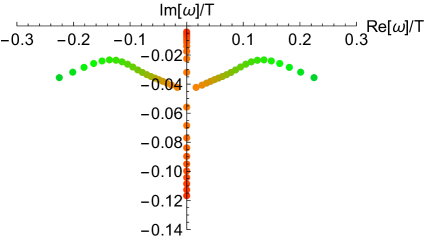
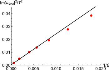
Figure 5: Left: The lowest two QNMs at zero momentum for $\mathcal{K}=-1/8$. We have fixed $\lambda=1\times 10^{-8}$ and $T/\sqrt{\rho}$ $\in$ [0.1, 0.4](green-red). Right: Collision frequency $Im\,\omega_{coll}$ as the function of $\beta=\langle SSB\rangle/\langle ESB\rangle$. We have fixed $\mathcal{K}=-1/8$, $\lambda$ $\in$ $[1\times 10^{-8},1\times 10^{-5}]$ and $\alpha/\sqrt{\rho}=1$. The black line indicates linear scaling.

In condensed matter systems, the presence of the phase relaxation could be attributed to either the proliferation of dislocations Delacrétaz et al. (2017) or the disorder effects Fukuyama (1978); Huse and Fogler (2000). And in holographic models, it is associated with the collision mechanism of the two lowest-lying quasi-normal modes Ammon et al. (2019a). It is worth studying the relationship between collision frequency $\omega_{coll}$ and characteristic parameter $\beta$. We can fix $\mathcal{K}$, choose one specific $\lambda$ and show the QNMs spectrum. Then identify the collision frequency at the collision point. The final results are shown in the right panel of Fig.5. For $\beta\gg 1$ the collision happens towards the origin so that very close to the origin, which can be described effectively by hydrodynamics. When $\beta=\infty$ (purely SSB case), the two modes are all located at the origin. As shown in the right panel of Fig.5, the collision frequency $\omega_{coll}$ shows proportional to the characteristic parameter $1/\beta$ approximately, that is

$$\frac{Im\,\omega_{coll}}{T}\sim\sqrt{\frac{\langle ESB\rangle}{\langle SSB\rangle}}.$$ (29)

Next we check Gell-Mann-Oakes-Renner (GMOR) relation which was originally found in QCD Gell-Mann et al. (1968) and later was also checked in holographic studies Kruczenski et al. (2004); Erlich et al. (2005); Filev et al. (2009); Argurio et al. (2016); Amoretti et al. (2017); Ammon et al. (2019a); Baggioli and Grieninger (2019). In the pseudo-spontaneous limit, the momentum relaxation rate can be neglected in (28). By reading QNMs data, phase relaxation rate $\Omega$ and pinning frequency $\omega_{0}$ can be identified. We show the dependence of the pinning frequency $\omega_{0}$ on the ESB and SSB scales in Fig.6. We find that the pinning frequency $\omega^{2}_{0}$ is proportional to the square root of the explicit breaking scale (24) and to the half to the third power of the spontaneous breaking scale (25). That said, in the pseudo-spontaneous limit, the results indicate the following scaling behavior

$$\omega^{2}_{0}\sim\sqrt{\langle ESB\rangle\langle SSB\rangle^{3}},$$ (30)

which is different from the original GMOR relation for Pion. Similarly in Andrade et al. (2018); Andrade and Krikun (2019); Andrade et al. (2021), they also obtained the results which is different from GMOR relation in holography. However in a simple holographic axion model, the authors proved this conclusion Ammon et al. (2019a).

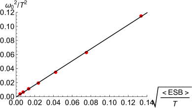
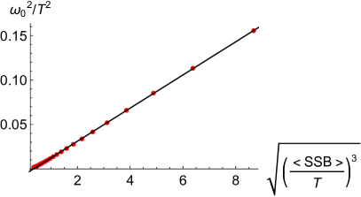
Figure 6: The dependence of the pinning frequency $\omega_{0}$ on the ESB and SSB scales. Left: We have fixed $\lambda$ $\in$ $[1\times 10^{-11},1\times 10^{-5}]$, $T/\sqrt{\rho}=0.15$, $\alpha/\sqrt{\rho}=1$ and $\mathcal{K}=-1/8$. Right: We have fixed $T/\sqrt{\rho}\in[0.06,0.30]$, $\alpha/\sqrt{\rho}=1$, $\lambda=1\times 10^{-8}$ and $\mathcal{K}=-1/8$. The black lines indicate linear scalings.

IV Electric conductivity

When the charge sector strongly couples with phonons, the combined system will reach local equilibrium extremally fast. Then, total momentum of the charge-phonon system should be conserved, resulting an infinite DC conductivity. Such a divergency of the conductivity can again be removed by introducing an ESB of translations which relaxes the momentum. However, unlike the picture without phonons, the AC conductivity now displays a finite peak at finite frequency. In this section, we turn to check how (pseudo-)phonons in our holographic model affect the charge transport in the purely SSB case and in the presence of weakly and explicitly broken translations, respectively.

IV.1 Purely SSB pattern

In the presence of purely SSB case, the AC conductivity at low frequency obeys the following hydrodynamic formula Hartnoll et al. (2016a)

$$\sigma(\omega)=\sigma_{Q}+\frac{\rho^{2}}{\chi_{PP}}\left(\delta(\omega)+\frac{i}{\omega}\right),$$ (31)

where $\sigma_{Q}$ is the so-called incoherent conductivity and $\rho^{2}/\chi_{PP}$ is Drude weight. Note that the DC conductivity is infinite in the SSB case because of the absence momentum relaxation mechanism. In this holographic model, the incoherent conductivity can be computed directly via the membrane paradigm (see Davison et al. (2015) for more details)

$$\sigma_{Q}=\left(1+\mathcal{K}\frac{4\pi\alpha^{2}}{s}\right)\left(\frac{sT}{sT+\mu\rho}\right)^{2}.$$ (32)

Here, the first law of thermodynamics $\epsilon+p=sT+\mu\rho$ has been applied.

We follow the procedure in Andrade and Withers (2014) to calculate AC conductivity at zero momentum by holographic method. Introduce the time-dependent perturbations around the background (6)

$$\delta g_{tx}=\frac{1}{u^{2}}h_{tx}(u)e^{-i\omega t},\quad\delta A_{x}=a_{x}(u)e^{-i\omega t},\quad\delta\phi_{x}=\phi_{x}(u)e^{-i\omega t},$$ (33)

and choose radial gauge $\delta g_{ux}=0$. The linearized equations of motion are given by

$$0=2f(\alpha^{2}u^{2}\mathcal{K}+1)^{2}(\rho u^{3}a_{x}^{\prime}-uh_{tx}^{\prime\prime}+2h_{tx}^{\prime})+\alpha^{2}uh_{tx}(2\lambda(\alpha^{2}u^{2}\mathcal{K}+1)^{2}-\rho^{2}u^{4}\mathcal{K})$$

$$+i\alpha u\phi_{x}\omega(2\lambda(\alpha^{2}u^{2}\mathcal{K}+1)^{2}-\rho^{2}u^{4}\mathcal{K}),$$ (34)

$$0=2i\rho\omega a_{x}(\alpha^{2}u^{3}\mathcal{K}+u)^{2}+\alpha f\phi_{x}^{\prime}(2\lambda(\alpha^{2}u^{2}\mathcal{K}+1)^{2}-\rho^{2}u^{4}\mathcal{K})-2i\omega h_{tx}^{\prime}(\alpha^{2}u^{2}\mathcal{K}+1)^{2},$$ (35)

$$0=\omega^{2}a_{x}(-(\alpha^{2}u^{2}\mathcal{K}+1))-f(a_{x}^{\prime}(\alpha^{2}u\mathcal{K}(uf^{\prime}+2f)+f^{\prime})+fa_{x}^{\prime\prime}(\alpha^{2}u^{2}\mathcal{K}+1)-\rho h_{tx}^{\prime}),$$ (36)

$$0=f(\phi_{x}^{\prime}(2f(2\lambda(\alpha^{2}u^{2}\mathcal{K}+1)^{3}+\rho^{2}u^{4}\mathcal{K}(1-\alpha^{2}u^{2}\mathcal{K}))-uf^{\prime}(\alpha^{2}u^{2}\mathcal{K}+1)(2\lambda(\alpha^{2}u^{2}\mathcal{K}+1)^{2}$$

$$-\rho^{2}u^{4}\mathcal{K}))-fu\phi_{x}^{\prime\prime}(\alpha^{2}u^{2}\mathcal{K}+1)(2\lambda(\alpha^{2}u^{2}\mathcal{K}+1)^{2}-\rho^{2}u^{4}\mathcal{K}))-u\phi_{x}\omega^{2}(\alpha^{2}u^{2}\mathcal{K}+1)(2\lambda(\alpha^{2}u^{2}\mathcal{K}+1)^{2}$$

$$-\rho^{2}u^{4}\mathcal{K})+i\alpha u\omega h_{tx}(\alpha^{2}u^{2}\mathcal{K}+1)(2\lambda(\alpha^{2}u^{2}\mathcal{K}+1)^{2}-\rho^{2}u^{4}\mathcal{K}).$$ (37)

It is easy to check there are three independent equations above. One can reduce them to two equations (see Wang et al. (2019) for analogous simplification method). The AC conductivity can be computed by solving (34-37) numerically via Kubo formula Ammon et al. (2019a)

$$\sigma(\omega)=\frac{1}{i\omega}\mathcal{G}_{JJ}^{R}(\omega,k=0).$$ (38)

We show that the numerical results of AC and incoherent conductivities in Fig.7. These results imply that the background solution of scalar field $\phi^{I}=\alpha x^{I}$ should be interpreted as the SSB nature. Moreover, the incoherent conductivity is also controlled by $\alpha$ and coupling $\mathcal{K}$, which can be viewed as the effect from phonons. Note that this can never happen if we neglect the direct coupling the gauge field and the axions in the bulk theory. It is obvious to see in Fig.7 that our numerical results from (38) are in agreement with analytical results from (31-32) .

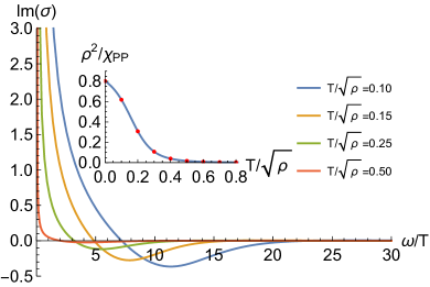
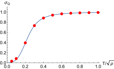
Figure 7: Left: The imaginary parts of AC conductivity for different temperatures. The inset plot shows the Drude weight $\rho^{2}/\chi_{PP}$. Blue line is the analytical result obtained from (31) and red dots are the numerical results from (38). Right: The incoherent conductivity $\sigma_{Q}$ as the function of temperature. Blue line is the analytical result obtained from (32) and red dots are the numerical results from (38) . We have fixed $\mathcal{K}=-1/8$ and $\lambda=0$.

IV.2 Pinned structure

In section III.2, we study the pinned phonons by turning on small external source. In this case, the DC conductivity can be computed anatically by the membrane paradigm Donos and Gauntlett (2014c); Baggioli et al. (2017)

$$\sigma_{DC}=1+\mathcal{K}\alpha^{2}u_{h}^{2}+\frac{\rho^{2}u_{h}^{2}}{\alpha^{2}\left(\lambda-\frac{\mathcal{K}\rho^{2}u_{h}^{4}}{2\left(1+\mathcal{K}\alpha^{2}u_{h}^{2}\right)^{2}}\right)}.$$ (39)

The structure of the pinned phonons are also captured by the AC conductivity in the low frequency. AC conductivity (31) from hydrodynamics should be modified in the presence of both ESB and SSB, which is given by Amoretti et al. (2020a, 2019b)

$$\sigma(\omega)=\sigma_{Q}+\frac{\gamma_{1}^{2}\chi_{PP}^{2}\omega_{0}^{2}(\Gamma-i\omega)+2\gamma_{1}\rho\chi_{PP}\omega_{0}^{2}+\rho^{2}(\Omega-i\omega)}{\chi_{PP}^{2}(\left(\Omega-i\omega)(\Gamma-i\omega\right)+\omega_{0}^{2})}.$$ (40)

where $\gamma_{1}$ is the coefficient which is extracted from the correlator between the electric current and Goldstone operator. When the momentum relaxation is slow, relaxation rate $\Gamma$ can be ignored. Based on our calculation, $\omega_{0}^{2}$ is the very small quantity. Thus we can omit the contribution of the $\gamma_{1}$ term. We identify $\Omega$ and $\omega_{0}$ by extracting QNMs data, which will fix all the parameters (40), to fit the AC conductivity by holography. The results are shown in Fig.8. We observe that the numerical AC conductivities are fitted by the hydrodynamic predictions well. As the authors point out Baggioli and Pujolas (2017); Goutéraux et al. (2016); An et al. (2020), the pinning effect introduces the metal-insulator transition. From the perspective of the shear viscosity, there is no specific behaviour at both sides of the transition point (see Appendix C for more details).

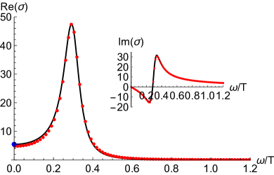
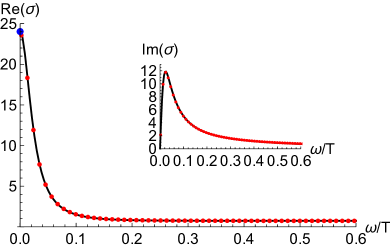
Figure 8: Comparisons between numerical AC conductivities (black solid lines) and hydrodynamic predictions (red dots) for different temperatures. The blue dots are the DC conductivity results from (39). Left: $T/\sqrt{\rho}=0.1$ and $\omega_{0}^{2}\approx 0.0017$. Here, one should distinguish $\omega_{0}$-the mass of pinned phonons and $\omega_{\text{peak}}$, the peak of the conductivity in IR region. Right: $T/\sqrt{\rho}=0.3$. We have fixed $\lambda=1\times 10^{-7}$ and $\mathcal{K}=-1/8$.

V Conclusions

In this work, we consider a holographic model that can break translational invariance in the dual field theory. We confirm the explicit breaking by turning on the linear axion term $\lambda X$ and spontaneous breaking by a gauge-axion coupling $\mathcal{K}XF^{2}$ via the UV analysis.

When turning off the external source, we compute shear modulus and viscosity by holography. The non-trivial results imply that the dual boundary system is an elastic solid. By calculating quasi-normal modes and making a comparison with the hydrodynamics predictions, we verify the existence of the gapless transverse phonons in the low energy spectrum. Then we turn on the slow momentum relaxation to see pinned phonons and check GMOR relation. It is found that the pinning frequency is proportional to the square root of the explicit breaking scale and to the half to the third power of the spontaneous breaking scale. This implies that it is different from the “standard” GMOR relation in our model.

We then study the charge transport. Firstly in the purely SSB pattern, the AC conductivity is in perfect agreement with the hydrodynamics expectations. This allows us to claim that the background solution of scalar field should be interpreted as the SSB contribution. Meanwhile in the presence of weakly explicit breaking, we show that the numerical AC conductivity can also be fitted by the hydrodynamic predictions well.

In the small frequency and momentum regime, our model shares the same hydrodynamic formulas with other holographic axion models Baggioli et al. (2021) or the homogeneous models with more complicated setups Amoretti et al. (2019b); Andrade et al. (2018) (even though the coefficients and parameters in the hydrodynamic formulation depend on the setup). This again verifies the statement that hydrodynamics provides a universal description for strongly coupled systems.

In this paper we only focus on the transverse channel of the system. The spectra of the longitudinal channel are also worth analyzing. This channel contains a pair of sound modes and one crystal diffusion mode in the low momentum limit, which is more complicated Ammon et al. (2019b); Baggioli et al. (2019); Baggioli and Grieninger (2019). We can study how charge density affects speed of longitudinal sounds, crystal diffusion and check the universality of its lower Baggioli and Li (2020); Wu et al. (2021) and upper Baggioli and Li (2020); Arean et al. (2020); Wu et al. (2021) bounds proposed previously. In addition, one can also investigate the magnetic effect with the current model and compare the result with that from the magneto-hydrodynamics Amoretti et al. (2020b); Delacrétaz et al. (2019) and other holographic models with magnetic effects Baggioli et al. (2020a); Amoretti et al. (2020c, 2021); Donos et al. (2021). We will leave these for future work.

Appendix A Derivation details for analytical Green’s functions

In this appendix, we show the details for the analytical calculations of Green’s functions $\mathcal{G}_{T_{xy}T_{xy}}^{R}$ at high and zero temperature limits.

A.1 High temperature limit

Let us focus on the high temperature limit first, i.e. $\sqrt{\rho}/T\ll 1$ that is equivalent to small charge density limit. We use Poincaré coordinates (6) this time and turn on shear perturbation $\delta g_{xy}=e^{-i\omega t}h(u)/u^{2}$. The perturbation equation is given by

$$h^{\prime\prime}+\left(\frac{f^{\prime}}{f}-\frac{2}{u}\right)h^{\prime}+\left(\frac{\omega^{2}}{f^{2}}+\frac{\alpha^{2}\hat{\rho}^{2}T^{4}u^{4}\mathcal{K}}{2f\left(\alpha^{2}u^{2}\mathcal{K}+1\right)^{2}}\right)h=0,$$ (41)

where we have introduced a dimensionless parameter which is defined by

$$\hat{\rho}=\left(\frac{\sqrt{\rho}}{T}\right)^{2}.$$ (42)

First, we show the analytical procedure for the correlator (16). To solve the equation of motion (41), one should implement the infalling boundary condition at the horizon and require field $h(u=0)=h_{0}$ at the AdS boundary in zero frequency limit. The on-shell action can be obtained Alberte et al. (2016b)

$$S_{bdy}=\int d^{2}x\int\frac{d\omega}{2\pi}h_{0}\mathcal{F}(\omega,u)h_{0}\bigg{|}_{u=\epsilon},$$ (43)

where $\epsilon$ is the UV cut-off and $h_{0}$ is the value of the bulk field $h$ at the boundary, which is equivalent to the source $h_{0}\equiv h(u=0).$ As illustrated in Son and Starinets (2002), the retarded Green’s function $\mathcal{G}^{R}_{T_{ij}{T_{ij}}}$ can be computed by taking two functional derivative of the above on-shell action with respect to the source $h_{0}$

$$\mathcal{G}^{R}_{T_{ij}{T_{ij}}}=-\lim_{\epsilon\rightarrow 0}2\mathcal{F}(\omega,u)\bigg{|}_{u=\epsilon}.$$ (44)

The equation (41) can be solved by imposing the follow ansatz

$$h(u)=h_{0}\,e^{-\frac{i\omega}{4\pi T}logf}\left(\Phi_{0}(u)+\frac{i\omega}{4\pi T}\Phi_{1}(u)+\cdots\right),$$ (45)

where exponential prefactor represents infalling behaviour and ellipsis denotes higher frequency contributions which are neglected. The functions $\Phi_{0}$ and $\Phi_{1}$ are required to be regular. We set

$$\Phi_{0}(0)=1,\qquad\Phi_{1}(0)=0,$$ (46)

near the boundary.

One can use perturbative method to solve the equation (41) with the ansatz (45). The equations for $\Phi_{0}$ and $\Phi_{1}$ can be obtained order by order in the frequency

$$0=\left(\frac{f}{u^{2}}\Phi_{0}^{\prime}(u)\right)^{\prime}+\frac{\alpha^{2}\hat{\rho}^{2}T^{4}u^{2}\mathcal{K}}{2\left(\alpha^{2}u^{2}\mathcal{K}+1\right)^{2}}\Phi_{0}(u),$$

$$0=\left(\frac{f}{u^{2}}\Phi_{1}^{\prime}(u)\right)^{\prime}+\frac{\alpha^{2}\hat{\rho}^{2}T^{4}u^{2}\mathcal{K}}{2\left(\alpha^{2}u^{2}\mathcal{K}+1\right)^{2}}\Phi_{1}(u)-\frac{2f^{\prime}}{u^{2}}\Phi_{0}^{\prime}(u)+\left(\frac{2f^{\prime}}{u^{3}}-\frac{f^{\prime\prime}}{u^{2}}\right)\Phi_{0}(u).$$ (47)

Since we consider small charge density limit, the emblackening factor $f$ can be simplified to Schwarzchild-AdS geometry $f(u)=1-u^{3}/u_{h}^{3}$ and the Hawking temperature is $T=3/(4\pi u_{h})$. Meanwhile, we adopt the following series expansions for the ansatz (45) in $\hat{\rho}^{2}$

$$\Phi_{0}=\sum_{n=0}^{\infty}\hat{\rho}^{2n}\phi_{n},\qquad\Phi_{1}=\sum_{n=0}^{\infty}\hat{\rho}^{2n}\psi_{n},$$ (48)

where the requirements (46) for $\Phi_{0}$ and $\Phi_{1}$ make $\phi_{0}=1$ and $\psi_{0}=0$. Substitute the above expansions into (47), and one can obtain

$$\left(\frac{f}{u^{2}}\phi_{1}^{\prime}\right)^{\prime}=-\frac{\alpha^{2}u^{2}\mathcal{K}T^{4}}{2\left(\alpha^{2}u^{2}\mathcal{K}+1\right)^{2}}\approx-\frac{1}{2}\alpha^{2}u^{2}\mathcal{K}T^{4},$$ (49)

$$\left(\frac{f}{u^{2}}\psi_{1}^{\prime}\right)^{\prime}=2\frac{f^{\prime}}{u^{2}}\phi_{1}^{\prime}.$$ (50)

By dimensional analysis, the dimension of $\alpha$ is the same as $\sqrt{\rho}$. We can expand $\alpha$ to get the leading order contribution, i.e. approximate term in (49).

The on-shell action is given by Alberte et al. (2016b)

$$S_{bdy}=-\frac{1}{2}\int d^{3}x\left(\frac{f}{u^{2}}h(u)h^{\prime}(u)\right)\bigg{|}_{u=\epsilon}^{u=uh},$$ (51)

where $\epsilon$ is the UV cut-off. Expand the above formula at leading order in the charge density and frequency

$$S_{bdy}=-\int d^{3}x\,\frac{h_{0}^{2}}{2}\left[\hat{\rho}^{2}\left(\frac{f}{\epsilon^{2}}\phi_{1}^{\prime}\right)+\frac{i\omega}{4\pi T}\left(\frac{3}{u_{h}^{3}}+\hat{\rho}^{2}\left(\frac{f}{\epsilon^{2}}\psi_{1}^{\prime}\right)-2\hat{\rho}^{2}log\,f\left(\frac{f}{\epsilon^{2}}\phi_{1}^{\prime}\right)\right)+\cdots\right].$$ (52)

The shear elastic modulus and viscosity can be calculated according to (43-44) and (52)

$$G=Re\mathcal{G}_{T_{xy}T_{xy}}^{R}=\lim_{\epsilon\rightarrow 0}\hat{\rho}^{2}\left(\frac{f}{\epsilon^{2}}\phi_{1}^{\prime}\right),$$ (53)

$$\eta=\lim_{\omega\rightarrow 0}\left[-\frac{1}{\omega}Im\mathcal{G}_{T_{xy}T_{xy}}^{R}(\omega)\right]=\lim_{\epsilon\rightarrow 0}\frac{1}{4\pi T}\left(\frac{3}{u_{h}^{3}}+\hat{\rho}^{2}\left(\frac{f}{\epsilon^{2}}\psi_{1}^{\prime}\right)\right).$$ (54)

Firstly, we compute the shear elastic modulus concretely by using (49)

$$G=\hat{\rho}^{2}\lim_{\epsilon\rightarrow 0}\int^{u_{h}}_{\epsilon}\left(-\frac{1}{2}\alpha^{2}u^{2}\mathcal{K}T^{4}\right)$$

$$\,\,\,\,\,=-\frac{1}{6}\alpha^{2}\hat{\rho}^{2}T^{4}\mathcal{K}u_{h}^{3}.$$ (55)

We recover the parameter $\rho$ and replace $u_{h}$ with $T$. Then one can re-write the above relation

$$G=-\frac{9\mathcal{K}\alpha^{2}T}{128\pi^{3}}\left(\frac{\sqrt{\rho}}{T}\right)^{4}+\cdots.$$ (56)

Secondly, we show the shear viscosity. In small charge density limit, the equation (49) for $\phi_{1}$ is solved by

$$\frac{f}{u^{2}}\phi_{1}^{\prime}=\frac{1}{6}\alpha^{2}T^{4}\mathcal{K}\left(u^{3}-u_{h}^{3}\right),$$ (57)

For (50) and (57),

$$\frac{f}{u^{2}}\psi_{1}^{\prime}=\int_{u}^{u_{h}}2\frac{f^{\prime}}{x^{2}}\phi_{1}^{\prime}dx=\int_{u}^{u_{h}}2\frac{f^{\prime}}{f}\left(\frac{f}{x^{2}}\phi_{1}^{\prime}\right)dx=\frac{1}{3}\alpha^{2}T^{4}\mathcal{K}\left(u_{h}^{3}-u^{3}\right).$$ (58)

Thus the ratio of shear viscosity $\eta$ to entropy density $s$ is

$$\frac{\eta}{s} =\lim_{\epsilon\rightarrow 0}\frac{1}{4\pi Ts}\left(\frac{3}{u_{h}^{3}}+\hat{\rho}^{2}\left(\frac{f}{\epsilon^{2}}\psi_{1}^{\prime}\right)\right)$$ (59)

$$=\frac{1}{4\pi}+\frac{81\mathcal{K}\alpha^{2}\rho^{2}}{16384\pi^{7}T^{6}},$$ (60)

where we have used simple emblackening factor $f(u)=1-u^{3}/u_{h}^{3}$, temperature $T=3/(4\pi u_{h})$ and entropy density $s=4\pi/u_{h}^{2}$. Thus the above formula can be re-written

$$\frac{\eta}{s}=\frac{1}{4\pi}+\frac{81\mathcal{K}\alpha^{2}}{16384\pi^{7}T^{2}}\left(\frac{\sqrt{\rho}}{T}\right)^{4}+\cdots.$$ (61)

The comparison between the numerical and analytical results for shear elastic modulus and viscosity is shown in Fig.9.

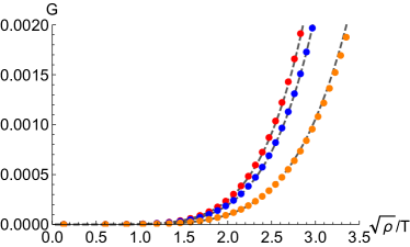
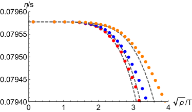
Figure 9: The comparison between the numerical and analytical results of shear elastic modulus and viscosity in the high temperature limit for $\mathcal{K}\in[-1/8,-1/20]$(red-orange). The dots are numerical results obtained by (16). The gray dashed lines are analytical results obtained by (56) and (61). We have fixed $\lambda=0$ and $\alpha/\sqrt{\rho}=1$.

A.2 Zero temperature limit

Next, we will consider $\eta/s$ ratio at zero temperature limit analytically. In this case (6), the black hole becomes extreme and the near-horizon geometry is $AdS_{2}\times R_{2}$ Baggioli (2019). The equation is given by

$$h^{\prime\prime}+\left(\frac{f^{\prime}}{f}-\frac{2}{u}\right)h^{\prime}+\left(\frac{\omega^{2}}{f^{2}}+\frac{\alpha^{2}\rho^{2}u^{4}\mathcal{K}}{2f\left(\alpha^{2}u^{2}\mathcal{K}+1\right)^{2}}\right)h=0,$$ (62)

where we have recovered the parameter $\rho$. We follow the method in Baggioli (2019). Assume a power-law ansatz for the field $h$

$$h(u)\sim(u-u_{h})^{\nu}.$$ (63)

The perturbation equation around the near-horizon geometry is

$$\nu\left((\nu-1)u_{h}+2u_{h}\right)f^{\prime\prime}\left(u_{h}\right)\left(\alpha^{2}\mathcal{K}u_{h}^{2}+1\right){}^{2}+\alpha^{2}\rho^{2}\mathcal{K}u_{h}^{5}=0.$$ (64)

One can get

$$\nu=-\frac{1}{2}\pm\xi,\qquad\xi\equiv\frac{1}{2}\sqrt{1-\frac{4\alpha^{2}\rho^{2}\mathcal{K}u_{h}^{4}}{\left(\alpha^{2}\mathcal{K}u_{h}^{2}+1\right)^{2}f^{\prime\prime}\left(u_{h}\right)}}.$$ (65)

Thus we can write the general solution

$$h(u)\sim u^{-1/2-\xi}+\mathcal{G}_{T_{xy}T_{xy}}(\omega)u^{-1/2+\xi}.$$ (66)

By dimensional analysis, frequency has the dimension of the temperature and the inverse of the radial coordinate ($\omega\sim T\sim u^{-1}$). This implies

$$\omega^{1/2+\xi}\sim\mathcal{G}_{T_{xy}T_{xy}}(\omega)\,\omega^{1/2-\xi},$$ (67)

and again

$$\mathcal{G}_{T_{xy}T_{xy}}(\omega)\sim\omega^{2\xi}.$$ (68)

Therefore

$$\eta\sim T^{2\xi-1}.$$ (69)

Finally we can obtain

$$\frac{\eta}{s}\sim T^{2\xi-1}.$$ (70)

Next we analyze $\xi$. In zero temperature limit, one can get

$$f^{\prime\prime}\left(u_{h}\right)=-\frac{6}{u_{h}^{2}}-\frac{\alpha^{2}\rho^{2}\mathcal{K}u_{h}^{4}}{2\left(\alpha^{2}\mathcal{K}u_{h}^{2}+1\right){}^{2}}+\frac{3\rho^{2}u_{h}^{2}}{2\left(\alpha^{2}\mathcal{K}u_{h}^{2}+1\right)}.$$ (71)

We set $u_{h}=1$ and $\alpha/\sqrt{\rho}=1$. Zero temperature limit gives another formula

$$\rho=2\sqrt{9\mathcal{K}^{2}+3}+6\mathcal{K}.$$ (72)

Substitute the above relations into (65), we can finally obtain the $\eta/s$ ratio at zero temperature limit

$$\frac{\eta}{s}\sim\left(\frac{T}{\sqrt{\rho}}\right)^{2\xi-1},\qquad\xi=\frac{1}{2}\sqrt{1-\frac{8\sqrt{3}\mathcal{K}}{\sqrt{3\mathcal{K}^{2}+1}}}.$$ (73)

We show the comparisons of the ratio obtained analytically and numerically in Fig.10.

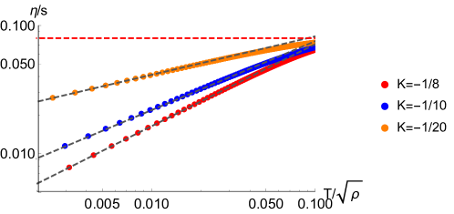
Figure 10: The $\eta/s$ ratio as the function of $T/\sqrt{\rho}$ for $\mathcal{K}\in[-1/8,-1/20]$(red-orange). The dots are numerical results obtained by (16). The black dashed lines are analytical results obtained by (73) in the low temperature limit. The red dashed line is the KSS bound. We have fixed coupling $\lambda=0$.

Appendix B Perturbation equations and Green’s functions

For convenience in numerical calculations of QNMs, we choose Eddington-Finkelstein (EF) coordinates

$$ds^{2}=\frac{1}{u^{2}}\left[-f(u)dt^{2}-2dtdu+dx^{2}+dy^{2}\right].$$ (74)

Since the boundary field theory is isotropic, we choose the momentum $k$ to be parallel to the $y$-axis. Take the following forms of the transverse perturbations

$$\delta g_{tx}=\frac{1}{u^{2}}h_{tx}(u)e^{-i\omega t+iky},\,\delta g_{xy}=\frac{1}{u^{2}}h_{xy}(u)e^{-i\omega t+iky},\,\delta A_{x}=a_{x}(u)e^{-i\omega t+iky},\,\delta\phi_{x}=\phi_{x}(u)e^{-i\omega t+iky},$$ (75)

and choose radial gauge $\delta g_{ux}=0$ for simplicity.

The equations are

$$0=u(2ikh_{xy}^{\prime}(\alpha^{2}u^{2}\mathcal{K}+1)^{2}-2h_{tx}^{\prime\prime}(\alpha^{2}u^{2}\mathcal{K}+1)^{2}+\alpha\phi_{x}^{\prime}(\rho^{2}u^{4}\mathcal{K}-2\lambda(\alpha^{2}u^{2}\mathcal{K}+1)^{2}))$$

$$+4h_{tx}^{\prime}(\alpha^{2}u^{2}\mathcal{K}+1)^{2}+2\rho u^{3}a_{x}^{\prime}(\alpha^{2}u^{2}\mathcal{K}+1)^{2},$$ (76)

$$0=2i\rho\omega a_{x}(\alpha^{2}u^{3}\mathcal{K}+u)^{2}+i(\alpha\phi_{x}\omega(2\lambda(\alpha^{2}u^{2}\mathcal{K}+1)^{2}-\rho^{2}u^{4}\mathcal{K})-2(\alpha^{2}u^{2}\mathcal{K}+1)^{2}(fkh_{xy}^{\prime}+\omega h_{tx}^{\prime}))$$

$$+\alpha f\phi_{x}^{\prime}(2\lambda(\alpha^{2}u^{2}\mathcal{K}+1)^{2}-\rho^{2}u^{4}\mathcal{K})+h_{tx}(2(\alpha^{2}\lambda+k^{2})(\alpha^{2}u^{2}\mathcal{K}+1)^{2}-\alpha^{2}\rho^{2}u^{4}\mathcal{K})$$

$$+2k\omega h_{xy}(\alpha^{2}u^{2}\mathcal{K}+1)^{2},$$ (77)

$$0=4ikh_{tx}(\alpha^{2}u^{2}\mathcal{K}+1)^{2}+h_{xy}(\alpha^{2}u(2\lambda(\alpha^{2}u^{2}\mathcal{K}+1)^{2}-\rho^{2}u^{4}\mathcal{K})+4i\omega(\alpha^{2}u^{2}\mathcal{K}+1)^{2})$$

$$-i(\alpha ku\phi_{x}(2\lambda(\alpha^{2}u^{2}\mathcal{K}+1)^{2}-\rho^{2}u^{4}\mathcal{K})+2(\alpha^{2}u^{2}\mathcal{K}+1)^{2}(h_{xy}^{\prime}(-iuf^{\prime}+2if+2u\omega)-ifuh_{xy}^{\prime\prime}+kuh_{tx}^{\prime})),$$ (78)

$$0=a_{x}^{\prime}(-2\alpha^{2}fu\mathcal{K}-i(2\omega-if^{\prime})(\alpha^{2}u^{2}\mathcal{K}+1))+a_{x}(k^{2}(\alpha^{2}u^{2}\mathcal{K}+1)-2i\alpha^{2}u\omega\mathcal{K})+\rho h_{tx}^{\prime}$$

$$-fa_{x}^{\prime\prime}(\alpha^{2}u^{2}\mathcal{K}+1),$$ (79)

$$0=-\phi_{x}(k^{2}u(\alpha^{2}u^{2}\mathcal{K}+1)(2\lambda(\alpha^{2}u^{2}\mathcal{K}+1)^{2}-\rho^{2}u^{4}\mathcal{K})+2i\omega(2\lambda(\alpha^{2}u^{2}\mathcal{K}+1)^{3}+\rho^{2}u^{4}\mathcal{K}(1-\alpha^{2}u^{2}\mathcal{K})))$$

$$+\phi_{x}^{\prime}(-2f(2\lambda(\alpha^{2}u^{2}\mathcal{K}+1)^{3}+\rho^{2}u^{4}\mathcal{K}(1-\alpha^{2}u^{2}\mathcal{K}))+u(f^{\prime}+2i\omega)(\alpha^{2}u^{2}\mathcal{K}+1)(2\lambda(\alpha^{2}u^{2}\mathcal{K}+1)^{2}-\rho^{2}u^{4}\mathcal{K}))$$

$$-2\alpha h_{tx}(2\lambda(\alpha^{2}u^{2}\mathcal{K}+1)^{3}+\rho^{2}u^{4}\mathcal{K}(1-\alpha^{2}u^{2}\mathcal{K}))-i\alpha kuh_{xy}(\alpha^{2}u^{2}\mathcal{K}+1)(2\lambda(\alpha^{2}u^{2}\mathcal{K}+1)^{2}-\rho^{2}u^{4}\mathcal{K})$$

$$+fu\phi_{x}^{\prime\prime}(\alpha^{2}u^{2}\mathcal{K}+1)(2\lambda(\alpha^{2}u^{2}\mathcal{K}+1)^{2}-\rho^{2}u^{4}\mathcal{K})+\alpha uh_{tx}^{\prime}(\alpha^{2}u^{2}\mathcal{K}+1)(2\lambda(\alpha^{2}u^{2}\mathcal{K}+1)^{2}-\rho^{2}u^{4}\mathcal{K}).$$ (80)

The asymptotic behaviour of the bulk fields near the boundary ($u=0$) are

$$h_{tx}=h_{tx(l)}(1+\dots)+h_{tx(s)}u^{3}(1+\dots),$$ (81)

$$h_{xy}=h_{xy(l)}(1+\dots)+h_{xy(s)}u^{3}(1+\dots),$$ (82)

$$a_{x}=a_{x(l)}(1+\dots)+a_{x(s)}u(1+\dots),$$ (83)

where $l$ and $s$ mark the leading and subleading orders. According to holographic dictionary and standard quantization, we can write the retarded Green’s functions as

$$\mathcal{G}^{R}_{T_{tx}T_{tx}}=\left(2\Delta-d\right)\frac{h_{tx(s)}}{h_{tx(l)}}=3\frac{h_{tx(s)}}{h_{tx(l)}},$$ (84)

$$\mathcal{G}^{R}_{T_{xy}T_{xy}}=\left(2\Delta-d\right)\frac{h_{xy(s)}}{h_{xy(l)}}=3\frac{h_{xy(s)}}{h_{xy(l)}},$$ (85)

$$\mathcal{G}^{R}_{JJ}=\frac{a_{x(s)}}{a_{x(l)}}.$$ (86)

The physical observables can be extracted from the retarded Green’s functions.

Appendix C DC conductivity and shear viscosity

We show the figures of DC conductivity and shear viscosity with temperature in Fig.11. As shown in the left figure, there exists the metal-insulator transition near the critical temperature $T/\sqrt{\rho}=0.265$. However there is no specific behaviour for the shear viscosity at both sides of the transition point.

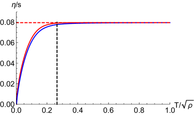
Figure 11: DC conductivity and $\eta/s$ as the function of the temperature. The black dashed line indicates the transition temperature. Left: $\mathcal{K}=-1/8$ and $\lambda=5\times 10^{-2}$. Right: $\mathcal{K}=-1/8$, $\lambda=0$ (red solid line) and $\lambda=5\times 10^{-2}$ (blue solid line).

References

- Teaney (2010) D. A. Teaney, “Viscous Hydrodynamics and the Quark Gluon Plasma,” in Quark-gluon plasma 4, edited by R. C. Hwa and X.-N. Wang (2010) arXiv:0905.2433 [nucl-th] .
- O’Hara et al. (2002) K. M. O’Hara, S. L. Hemmer, M. E. Gehm, S. R. Granade, and J. E. Thomas, Science 298, 2179 (2002), arXiv:0212463 [cond-mat] .
- Levitov and Falkovich (2016) L. Levitov and G. Falkovich, Nature Physics 12, 672 (2016), arXiv:1508.00836 [cond-mat] .
- Bandurin and et al (2016) D. A. Bandurin and et al, Science 351, 1055 (2016), arXiv:1509.04165 [cond-mat] .
- Kovtun (2012) P. Kovtun, J. Phys. A 45, 473001 (2012), arXiv:1205.5040 [hep-th] .
- Hartnoll (2009) S. A. Hartnoll, Class. Quant. Grav. 26, 224002 (2009), arXiv:0903.3246 [hep-th] .
- Natsuume (2015) M. Natsuume, AdS/CFT Duality User Guide, Vol. 903 (2015) arXiv:1409.3575 [hep-th] .
- (8) J. McGreevy, arXiv:1606.08953 [hep-th] .
- Hartnoll et al. (2016a) S. A. Hartnoll, A. Lucas, and S. Sachdev, (2016a), arXiv:1612.07324 [hep-th] .
- Horowitz et al. (2012a) G. T. Horowitz, J. E. Santos, and D. Tong, JHEP 07, 168 (2012a), arXiv:1204.0519 [hep-th] .
- Horowitz et al. (2012b) G. T. Horowitz, J. E. Santos, and D. Tong, JHEP 11, 102 (2012b), arXiv:1209.1098 [hep-th] .
- Donos and Hartnoll (2013) A. Donos and S. A. Hartnoll, Nature Phys. 9, 649 (2013), arXiv:1212.2998 [hep-th] .
- Vegh (2013) D. Vegh, (2013), arXiv:1301.0537 [hep-th] .
- Horowitz and Santos (2013) G. T. Horowitz and J. E. Santos, JHEP 06, 087 (2013), arXiv:1302.6586 [hep-th] .
- Blake and Tong (2013) M. Blake and D. Tong, Phys. Rev. D 88, 106004 (2013), arXiv:1308.4970 [hep-th] .
- Ling et al. (2013) Y. Ling, C. Niu, J.-P. Wu, and Z.-Y. Xian, JHEP 11, 006 (2013), arXiv:1309.4580 [hep-th] .
- Donos and Gauntlett (2014a) A. Donos and J. P. Gauntlett, JHEP 04, 040 (2014a), arXiv:1311.3292 [hep-th] .
- Andrade and Withers (2014) T. Andrade and B. Withers, JHEP 05, 101 (2014), arXiv:1311.5157 [hep-th] .
- Donos and Gauntlett (2014b) A. Donos and J. P. Gauntlett, JHEP 06, 007 (2014b), arXiv:1401.5077 [hep-th] .
- Goutéraux (2014) B. Goutéraux, JHEP 04, 181 (2014), arXiv:1401.5436 [hep-th] .
- Ling et al. (2015) Y. Ling, P. Liu, C. Niu, J.-P. Wu, and Z.-Y. Xian, JHEP 02, 059 (2015), arXiv:1410.6761 [hep-th] .
- Davison and Goutéraux (2015a) R. A. Davison and B. Goutéraux, JHEP 01, 039 (2015a), arXiv:1411.1062 [hep-th] .
- Donos and Pantelidou (2019) A. Donos and C. Pantelidou, JHEP 05, 079 (2019), arXiv:1903.05114 [hep-th] .
- Blake et al. (2014) M. Blake, D. Tong, and D. Vegh, Phys. Rev. Lett. 112, 071602 (2014), arXiv:1310.3832 [hep-th] .
- Baggioli and Pujolas (2015) M. Baggioli and O. Pujolas, Phys. Rev. Lett. 114, 251602 (2015), arXiv:1411.1003 [hep-th] .
- Alberte and Khmelnitsky (2015) L. Alberte and A. Khmelnitsky, Phys. Rev. D 91, 046006 (2015), arXiv:1411.3027 [hep-th] .
- Alberte et al. (2016a) L. Alberte, M. Baggioli, A. Khmelnitsky, and O. Pujolas, JHEP 02, 114 (2016a), arXiv:1510.09089 [hep-th] .
- Baggioli and Pujolas (2016) M. Baggioli and O. Pujolas, JHEP 12, 107 (2016), arXiv:1604.08915 [hep-th] .
- Alberte et al. (2018a) L. Alberte, M. Ammon, M. Baggioli, A. Jiménez, and O. Pujolàs, JHEP 01, 129 (2018a), arXiv:1708.08477 [hep-th] .
- Alberte et al. (2018b) L. Alberte, M. Ammon, A. Jiménez-Alba, M. Baggioli, and O. Pujolàs, Phys. Rev. Lett. 120, 171602 (2018b), arXiv:1711.03100 [hep-th] .
- Ammon et al. (2019a) M. Ammon, M. Baggioli, and A. Jiménez-Alba, JHEP 09, 124 (2019a), arXiv:1904.05785 [hep-th] .
- Ammon et al. (2019b) M. Ammon, M. Baggioli, S. Gray, and S. Grieninger, JHEP 10, 064 (2019b), arXiv:1905.09164 [hep-th] .
- Baggioli and Grieninger (2019) M. Baggioli and S. Grieninger, JHEP 10, 235 (2019), arXiv:1905.09488 [hep-th] .
- Baggioli et al. (2021) M. Baggioli, K.-Y. Kim, L. Li, and W.-J. Li, Sci. China Phys. Mech. Astron. 64, 270001 (2021), arXiv:2101.01892 [hep-th] .
- Goutéraux et al. (2016) B. Goutéraux, E. Kiritsis, and W.-J. Li, JHEP 04, 122 (2016), arXiv:1602.01067 [hep-th] .
- Baggioli et al. (2017) M. Baggioli, B. Goutéraux, E. Kiritsis, and W.-J. Li, JHEP 03, 170 (2017), arXiv:1612.05500 [hep-th] .
- Li and Wu (2019) W.-J. Li and J.-P. Wu, Eur. Phys. J. C 79, 243 (2019), arXiv:1808.03142 [hep-th] .
- Baggioli and Pujolas (2017) M. Baggioli and O. Pujolas, JHEP 01, 040 (2017), arXiv:1601.07897 [hep-th] .
- An et al. (2020) Y.-S. An, T. Ji, and L. Li, (2020), arXiv:2007.13918 [hep-th] .
- Amoretti et al. (2017) A. Amoretti, D. Areán, R. Argurio, D. Musso, and L. A. Pando Zayas, JHEP 05, 051 (2017), arXiv:1611.09344 [hep-th] .
- Amoretti et al. (2018a) A. Amoretti, D. Areán, B. Goutéraux, and D. Musso, Phys. Rev. D 97, 086017 (2018a), arXiv:1711.06610 [hep-th] .
- Amoretti et al. (2018b) A. Amoretti, D. Areán, B. Goutéraux, and D. Musso, Phys. Rev. Lett. 120, 171603 (2018b), arXiv:1712.07994 [hep-th] .
- Amoretti et al. (2019a) A. Amoretti, D. Areán, B. Goutéraux, and D. Musso, JHEP 10, 068 (2019a), arXiv:1904.11445 [hep-th] .
- Kim et al. (2014) K.-Y. Kim, K. K. Kim, Y. Seo, and S.-J. Sin, JHEP 12, 170 (2014), arXiv:1409.8346 [hep-th] .
- Kim et al. (2015) K.-Y. Kim, K. K. Kim, and M. Park, JHEP 04, 152 (2015), arXiv:1501.00446 [hep-th] .
- Davison and Goutéraux (2015b) R. A. Davison and B. Goutéraux, JHEP 09, 090 (2015b), arXiv:1505.05092 [hep-th] .
- Blake et al. (2018) M. Blake, R. A. Davison, S. Grozdanov, and H. Liu, JHEP 10, 035 (2018), arXiv:1809.01169 [hep-th] .
- Zhou et al. (2020) Y.-T. Zhou, X.-M. Kuang, Y.-Z. Li, and J.-P. Wu, Phys. Rev. D 101, 106024 (2020), arXiv:1912.03479 [hep-th] .
- Donos et al. (2020) A. Donos, D. Martin, C. Pantelidou, and V. Ziogas, Class. Quant. Grav. 37, 045005 (2020), arXiv:1906.03132 [hep-th] .
- Amoretti et al. (2020a) A. Amoretti, D. Areán, B. Goutéraux, and D. Musso, JHEP 01, 058 (2020a), arXiv:1910.11330 [hep-th] .
- Baggioli et al. (2020a) M. Baggioli, S. Grieninger, and L. Li, JHEP 09, 037 (2020a), arXiv:2005.01725 [hep-th] .
- Leutwyler (1997) H. Leutwyler, Helv. Phys. Acta 70, 275 (1997), arXiv:hep-ph/9609466 .
- Dubovsky et al. (2006) S. Dubovsky, T. Gregoire, A. Nicolis, and R. Rattazzi, JHEP 03, 025 (2006), arXiv:hep-th/0512260 .
- Nicolis et al. (2015) A. Nicolis, R. Penco, F. Piazza, and R. Rattazzi, JHEP 06, 155 (2015), arXiv:1501.03845 [hep-th] .
- Delacrétaz et al. (2017) L. V. Delacrétaz, B. Goutéraux, S. A. Hartnoll, and A. Karlsson, Phys. Rev. B 96, 195128 (2017), arXiv:1702.05104 [cond-mat.str-el] .
- Alberte et al. (2019) L. Alberte, M. Baggioli, V. C. Castillo, and O. Pujolas, Phys. Rev. D 100, 065015 (2019), arXiv:1807.07474 [hep-th] .
- Musso (2019) D. Musso, Eur. Phys. J. C 79, 986 (2019), arXiv:1810.01799 [hep-th] .
- Baggioli et al. (2020b) M. Baggioli, M. Vasin, V. V. Brazhkin, and K. Trachenko, Phys. Rept. 865, 1 (2020b), arXiv:1904.01419 [cond-mat.stat-mech] .
- Kovtun et al. (2005) P. Kovtun, D. T. Son, and A. O. Starinets, Phys. Rev. Lett. 94, 111601 (2005), arXiv:hep-th/0405231 .
- Baggioli (2019) M. Baggioli, Applied Holography: A Practical Mini-Course, SpringerBriefs in Physics (Springer, 2019) arXiv:1908.02667 [hep-th] .
- Hartnoll et al. (2016b) S. A. Hartnoll, D. M. Ramirez, and J. E. Santos, JHEP 03, 170 (2016b), arXiv:1601.02757 [hep-th] .
- Ling et al. (2016) Y. Ling, Z.-Y. Xian, and Z. Zhou, JHEP 11, 007 (2016), arXiv:1605.03879 [hep-th] .
- Jansen (2017) A. Jansen, Eur. Phys. J. Plus 132, 546 (2017), arXiv:1709.09178 [gr-qc] .
- Davison (2013) R. A. Davison, Phys. Rev. D 88, 086003 (2013), arXiv:1306.5792 [hep-th] .
- Fukuyama (1978) H. Fukuyama, Journal of the Physical Society of Japan 45, 1474 (1978).
- Huse and Fogler (2000) D. A. Huse and M. K. Fogler, Phys. Rev. B 62, 7553 (2000).
- Gell-Mann et al. (1968) M. Gell-Mann, R. J. Oakes, and B. Renner, Phys. Rev. 175, 2195 (1968).
- Kruczenski et al. (2004) M. Kruczenski, D. Mateos, R. C. Myers, and D. J. Winters, JHEP 05, 041 (2004), arXiv:hep-th/0311270 .
- Erlich et al. (2005) J. Erlich, E. Katz, D. T. Son, and M. A. Stephanov, Phys. Rev. Lett. 95, 261602 (2005), arXiv:hep-ph/0501128 .
- Filev et al. (2009) V. G. Filev, C. V. Johnson, and J. P. Shock, JHEP 08, 013 (2009), arXiv:0903.5345 [hep-th] .
- Argurio et al. (2016) R. Argurio, A. Marzolla, A. Mezzalira, and D. Musso, JHEP 03, 012 (2016), arXiv:1512.03750 [hep-th] .
- Andrade et al. (2018) T. Andrade, M. Baggioli, A. Krikun, and N. Poovuttikul, JHEP 02, 085 (2018), arXiv:1708.08306 [hep-th] .
- Andrade and Krikun (2019) T. Andrade and A. Krikun, JHEP 05, 119 (2019), arXiv:1812.08132 [hep-th] .
- Andrade et al. (2021) T. Andrade, M. Baggioli, and A. Krikun, JHEP 03, 292 (2021), arXiv:2009.05551 [hep-th] .
- Davison et al. (2015) R. A. Davison, B. Goutéraux, and S. A. Hartnoll, JHEP 10, 112 (2015), arXiv:1507.07137 [hep-th] .
- Wang et al. (2019) X.-J. Wang, H.-S. Liu, and W.-J. Li, Eur. Phys. J. C 79, 932 (2019), arXiv:1909.00224 [hep-th] .
- Donos and Gauntlett (2014c) A. Donos and J. P. Gauntlett, JHEP 11, 081 (2014c), arXiv:1406.4742 [hep-th] .
- Amoretti et al. (2019b) A. Amoretti, D. Areán, B. Goutéraux, and D. Musso, Phys. Rev. Lett. 123, 211602 (2019b), arXiv:1812.08118 [hep-th] .
- Baggioli et al. (2019) M. Baggioli, U. Gran, A. J. Alba, M. Tornsö, and T. Zingg, JHEP 09, 013 (2019), arXiv:1905.00804 [hep-th] .
- Baggioli and Li (2020) M. Baggioli and W.-J. Li, SciPost Phys. 9, 007 (2020), arXiv:2005.06482 [hep-th] .
- Wu et al. (2021) N. Wu, M. Baggioli, and W.-J. Li, JHEP 05, 014 (2021), arXiv:2102.05810 [hep-th] .
- Arean et al. (2020) D. Arean, R. A. Davison, B. Goutéraux, and K. Suzuki, (2020), arXiv:2011.12301 [hep-th] .
- Amoretti et al. (2020b) A. Amoretti, M. Meinero, D. K. Brattan, F. Caglieris, E. Giannini, M. Affronte, C. Hess, B. Buechner, N. Magnoli, and M. Putti, Phys. Rev. Res. 2, 023387 (2020b), arXiv:1909.07991 [cond-mat.str-el] .
- Delacrétaz et al. (2019) L. V. Delacrétaz, B. Goutéraux, S. A. Hartnoll, and A. Karlsson, Phys. Rev. B 100, 085140 (2019), arXiv:1904.04872 [cond-mat.mes-hall] .
- Amoretti et al. (2020c) A. Amoretti, D. K. Brattan, N. Magnoli, and M. Scanavino, JHEP 08, 097 (2020c), arXiv:2005.09662 [hep-th] .
- Amoretti et al. (2021) A. Amoretti, D. Arean, D. K. Brattan, and N. Magnoli, JHEP 05, 027 (2021), arXiv:2101.05343 [hep-th] .
- Donos et al. (2021) A. Donos, C. Pantelidou, and V. Ziogas, JHEP 05, 270 (2021), arXiv:2101.06230 [hep-th] .
- Alberte et al. (2016b) L. Alberte, M. Baggioli, and O. Pujolas, JHEP 07, 074 (2016b), arXiv:1601.03384 [hep-th] .
- Son and Starinets (2002) D. T. Son and A. O. Starinets, JHEP 09, 042 (2002), arXiv:hep-th/0205051 .