Bilevel Programs Meet Deep Learning:
A Unifying View on Inference Learning Methods

Abstract

In this work we unify a number of inference learning methods, that are proposed in the literature as alternative training algorithms to the ones based on regular error back-propagation. These inference learning methods were developed with very diverse motivations, mainly aiming to enhance the biological plausibility of deep neural networks and to improve the intrinsic parallelism of training methods. We show that these superficially very different methods can all be obtained by successively applying a particular reformulation of bilevel optimization programs. As a by-product it becomes also evident that all considered inference learning methods include back-propagation as a special case, and therefore at least approximate error back-propagation in typical settings. Finally, we propose Fenchel back-propagation, that replaces the propagation of infinitesimal corrections performed in standard back-propagation with finite targets as the learning signal. Fenchel back-propagation can therefore be seen as an instance of learning via explicit target propagation.

1 Introduction

In this work we analyze several instances of inference learning methods and how these approaches can be obtained as suitable reformulations of deeply nested minimization problems. We use inference learning [36] as an umbrella term for all learning methods based on explicit optimization (inference) of hidden unit activations. Inference learning includes methods such as layered contrastive Hebbian learning (CHL, xie2003equivalence [39]), equilibrium propagation [35], lifted neural networks [8, 14, 21], and predictive coding networks (PCN, whittington2017approximation [38, 36]). In a nutshell, all these methods can be interpreted as certain mathematical reformulations of deeply nested optimization problems. Specifically, learning in layered feed-forward neural network can be stated as the following nested optimization problem,

$$\min_{\theta_{0},\dotsc,\theta_{L-1}}\ell(z_{L}^{*})\;\;\text{s.t. }\qquad z_{1}^{*}=\arg\min_{z_{1}}E_{1},(x,z_{1};\theta_{0})\qquad z_{k+1}^{*}=\arg\min_{z_{k+1}}E_{k}(z_{k}^{*},z_{k+1};\theta_{k})$$ (1)

for $k=1,\dotsc,L$. The values $(z_{k}^{*})_{k=1}^{L}$ are usually refered to as the network activations determined in a forward pass, and the collection $(\theta_{0},\dotsc,\theta_{L-1})$ are the trainable network parameters. The conversion between a DNN architecture and Eq. 1 is not unique. E.g., for ReLU-based DNNs the choice for $E_{k}$ can be $E_{k}(z_{k},z_{k+1};\theta_{k})=\left\lVert z_{k+1}-[\theta_{k}z_{k}]_{+}\right\rVert^{2}$ [8] or $E_{k}(z_{k},z_{k+1};\theta_{k})=\left\lVert z_{k+1}-\theta_{k}z_{k}\right\rVert^{2}+\imath_{\geq 0}(z_{k+1})$ [42], where $[\cdot]_{+}:=\max\{0,\cdot\}$ and $\imath_{C}$ is the extended valued characteristic function of a set $C$. In our work it will become clear, that the differences between inference learning methods is largely induced by different (but equivalent) choices for the underlying nested optimization problems and by selected direction for processing the nesting levels (top-down or bottom-up). Since all these approaches yield the standard back-propagation (BP) method at least as a limit case, understanding the connections between the inference learning methods may also provide insights into regular back-propagation. In particular, some inference learning methods can be interpreted as instances of target propagation [5, 20, 6, 29, 25]—where desired neural activations instead of (infinitesimal) error signals are propagated through the network—and as the basis for learning methods using layer-local losses (including [12, 2]), hence this work may also shed new light on those methods.

Method	$E_{k}$	Direction	Linearized outer loss	Inference
CHL	Fenchel	Bottom-up	No	Layer-convex
Convex CHL	Proximal	Bottom-up	No	Convex
FLN & LPOM	Fenchel/Proximal	Top-down	No	Layer-Convex
MAC	Penalizer	Any	No	Non-convex
BP & PCN	Penalizer	Top-down	Yes	Closed-form
Fenchel BP	Fenchel/Proximal	Top-down	Yes	Closed-form

Table 1: A taxonomy of inference learning methods unified in this work: Contrastive Hebbian learning (CHL, xie2003equivalence [39]) and convex CHL [40], Fenchel lifted networks (FLN, gu2018fenchel [14]) and lifted proximal operator machines (LPOM, li2018lifted [21]), method of auxiliary coordinates (MAC, carreira2014distributed [8]), back-propagation (BP) and predictive coding networks (PCN, whittington2017approximation [38, 36]). Fenchel back-propagation (Fenchel BP) is a generalization of standard back-propagation discussed in Section 4.2.

Table 1 summarizes the relations between inference learning methods. As it can be seen, the methods differ in the choice of $E_{k}$, the direction of unravelling the nesting levels, and whether an additional linearization step is applied. Typical choices for $E_{k}$ are given in column $E_{k}$, which can be based on a penalizer of the forward model $z_{k+1}=f_{k}(z_{k};\theta_{k})$, using convex (Fenchel) conjugates, $G_{k+1}(z_{k+1})-z_{k+1}^{\top}W_{k}z_{k}$, or proximal mappings, $\tfrac{1}{2}\left\lVert z_{k+1}-W_{k}z_{k}\right\rVert^{2}+F_{k+1}(z_{k+1})$. The last column indicates the difficulty of the resulting inference task needed to determine the network activations/targets. The different realizations have also an impact on the required level of synchronization points: BP and PCN use a dedicated forward and backward pass (which is relaxed in song2020can [36]), whereas CHL requires two global (free and clamped) but non-directed phases for learning. Lifted neural networks such as the method of auxiliary coordinates (MAC) [8] and lifted proximal operator machines (LPOM) [21] (and the closely related lifted Fenchel networks [14]) need local synchronization between layers due to the non-convexity of the underlying objective function. Fenchel back-propagation is an algorithm similar to back-propagation and is presented in Section 4.2.

Not all instances of inference learning methods belong to this taxonomy. One aspect that the above methods have in common is, that they include back-propagation as a limit case, which is violated e.g. for the inference learning methods proposed in [42, 3] (as demonstrated in zach2019contrastive [40]).

Our main contribution is establishing connections between certain reformulations for deeply nested optimization tasks and inference learning methods. Singly nested i.e. bilevel optimization has been leveraged in the machine learning literature for parameter learning in variational and dictionary-based models (e.g. mairal2011task [24, 18, 43]) and for meta-learning (such as bennett2008bilevel [7, 11, 32, 22]). The resulting optimization methods are often based on surrogates for the original bilevel optimization tasks using KKT conditions [7, 18, 43]. Unrolling a minimization problem is a common technique in machine learning to replace the inner optimization task with a finite sequence of local minimization steps [10, 23, 28, 11] (which is similar but not identical to back-propagation through time [37]). If the inner problem is twice differentiable, implicit differentiation is applicable for gradient-based optimization of the outer objective [31, 1, 17, 4, 34], which has been more recently extended to allow constraints in the inner problem [13].

2 Surrogates for Bilevel Programs

Since the learning problem in deep networks in Eq. 1 is a nested minimization task, we first consider singly nested i.e. bilevel problems. For an outer loss $\ell(\cdot)$ and inner objective $E(\cdot;\cdot)$ we introduce the bilevel minimization problem

$$\mathcal{L}(\theta):=\ell(z^{*})\qquad\text{s.t. }z^{*}=\arg\min\nolimits_{z}E(z;\theta),$$ (2)

where we assume that $E$ has a unique minimizer for each feasible value $\theta$. We also require that the outer loss $\ell$ is differentiable, bounded from below and that $\ell(z)<\infty$ for all $z$. The first step is to rewrite Eq. 2 using an optimal value reformulation for bilevel programs [30] (and see dempe2013bilevel [9] for a discussion of several reformulations for bilevel programs),

$$\min\nolimits_{\theta,z}\ell(z)\qquad\text{s.t. }E(z;\theta)\leq\min\nolimits_{z^{\prime}}E(z^{\prime};\theta),$$ (3)

The corresponding Lagrangian relaxation is (using $\beta^{-1}$ to parametrize the non-negative multiplier),

$$\max\nolimits_{\beta>0}\min\nolimits_{\theta,z}\ell(z)+\tfrac{1}{\beta}\big{(}E(z;\theta)-\min\nolimits_{z^{\prime}}E(z^{\prime};\theta)\big{)}.$$ (4)

By fixing a multiplier $\beta>0$ we arrive at the main quantity of interest in this work:

Definition 1.

The contrastive surrogate for the bilevel minimization problem in Eq. 2 is defined as follows,

$$\mathcal{L}^{\beta}(\theta) :=\min_{z}\big{\{}\ell(z)+\tfrac{1}{\beta}E(z;\theta)\big{\}}-\min_{z}\tfrac{1}{\beta}E(z;\theta)$$

$$=\ell(\hat{z}(\beta))+\tfrac{1}{\beta}E(\hat{z}(\beta);\theta)-\tfrac{1}{\beta}E(z^{*};\theta),$$ (5)

where $\beta>0$ is the “spacing parameter.” The minimizers of the two sub-problems are denoted as

$$\hat{z}(\beta) :=\arg\min\nolimits_{z}\beta\ell(z)+E(z;\theta)$$

$$z^{*} :=\arg\min\nolimits_{z}E(z;\theta),$$ (6)

where the dependence on $\theta$ is implicit.

For brevity we will often write $\hat{z}_{\beta}$ instead of $\hat{z}(\beta)$. We call this surrogate contrastive in analogy with e.g. contrastive Hebbian learning [27, 39] that relies on solving two minimization tasks; one to obtain a loss-augmented “clamped” solution and one for the “free” solution not using any information from the outer loss $\ell$. The contrastive surrogate is a “min-min-max” instance, as one aims to minimize w.r.t. $\theta$, but the two subproblems in $z$ have opposing signs. Fortunately, in our setting solving $\min_{z}E(z;\theta)$ is typically (but not always) easy and often has a closed-form solution. If $E(z;\theta)$ is convex in $z$, then one can obtain a “min-min-min” problem using duality [41].

Naturally, we are most interested in the setting when $\beta\approx 0$, where the contrastive surrogates are good approximations of the optimal value reformulation (Eq. 3), and it is therefore important to better understand the finite difference $\tfrac{1}{\beta}(E(\hat{z}_{\beta};\theta)-E(z^{*};\theta))$ in the limit $\beta\to 0^{+}$, i.e. $\frac{dE(\hat{z}_{\beta};\theta)}{d\beta}|_{\beta=0^{+}}$. If $E$ is differentiable w.r.t. $z$, then (by the chain rule) the relevant quantity to analyze is $\frac{d\hat{z}_{\beta}}{d\beta}|_{\beta=0^{+}}=\frac{d\hat{z}_{\beta}}{d\beta}|_{\beta=0}$ (due to strong differentiability). The simplest setting is when $\ell$ and $E$ are sufficiently regular:

Proposition 1.

If $\ell$ is differentiable and $E$ is twice continuously differentiable, then

$$\tfrac{d}{d\beta}\hat{z}(\beta)\big{|}_{\beta=0}=-\big{(}\tfrac{\partial^{2}}{\partial z^{2}}E(z^{*};\theta)\big{)}^{-1}\ell^{\prime}(z^{*})$$ (7)

and

$$\tfrac{d}{d\beta}E(\hat{z}(\beta);\theta)\big{|}_{\beta=0}\!=\!-\tfrac{\partial}{\partial z}E(z^{*};\theta)\big{(}\tfrac{\partial^{2}}{\partial z^{2}}E(z^{*};\theta)\big{)}^{-1}\ell^{\prime}(z^{*}).$$ (8)

The proof is based on implicit differentiation and is detailed (together with all following results) in the appendix. By taking the partial derivative w.r.t. $\theta$, we arrive at a familiar expression for gradient back-propagation through minimization [31, 1, 17, 4, 34],

$$\tfrac{d}{d\theta}\mathcal{L}(\theta) =-\!\tfrac{\partial^{2}}{\partial\theta\partial z}E(z^{*};\theta)\left(\tfrac{\partial^{2}}{\partial z^{2}}E(z^{*}(\theta);\theta)\right)^{-1}\ell^{\prime}(z^{*})$$

$$=\lim_{\beta\to 0^{+}}\tfrac{1}{\beta}\tfrac{\partial}{\partial\theta}\big{(}E(\hat{z}_{\beta};\theta)-E(z^{*};\theta)\big{)}.$$ (9)

Hence, we may facilitate gradient-based minimization of $\theta$ e.g. by choosing $\beta\approx 0$ and updating $\theta$ according to

$$\theta^{(t+1)}\leftarrow\theta^{(t)}-\tfrac{\eta^{(t)}}{\beta}\tfrac{\partial}{\partial\theta}\big{(}E(\hat{z}_{\beta};\theta)-E(z^{*};\theta)\big{)},$$ (10)

where $\eta^{(t)}$ is the learning rate at iteration $t$. With the assumptions given in Prop. 1 we know that in the limit $\beta\to 0^{+}$ we obtain an exact gradient method. Implicit differentiation can be extended to allow (smooth) constraints on $z$ in $E(z;\theta)$ [13]. One advantage of the surrogates in Def. 1 over implicit differentiation is, that the former requires only the directional derivative $\frac{d\hat{z}(\beta)}{d\beta}|_{\beta=0^{+}}$ to exist, which is a weaker requirement than existence of a strong derivative $dz^{*}(\theta)/d\theta$ as it can be seen in the following simple, but important example.

Example 1 (ReLU activation).

Let $E(z;\theta)$ be given as $E(z;\theta)=\tfrac{1}{2}\lVert z-\theta x\rVert^{2}+\imath_{\geq 0}(z)$ and $\ell(z)=g^{\top}z$. Then $z^{*}=[\theta x]_{+}$ and $\hat{z}_{\beta}=[\theta x-\beta g]_{+}$, and therefore

$$\frac{d\hat{z}_{\beta}}{d\beta}\big{|}_{\beta=0^{+}} =\lim_{\beta\to 0^{+}}\frac{[\theta x-\beta g]_{+}-[\theta x]_{+}}{\beta}=\mathtt{D}\,g,$$ (11)

where $\mathtt{D}$ is a diagonal matrix with

$$\mathtt{D}_{jj}=\begin{cases}{-1}&\text{if }(\theta x)_{j}>0\lor\big{(}(\theta x)_{j}=0\land g_{j}\geq 0\big{)}\\ 0&\text{if }(\theta x)_{j}<0\lor\big{(}(\theta x)_{j}=0\land g_{j}<0\big{)}.\end{cases}$$ (12)

Thus, the gradient w.r.t. $\theta$ is given by

$$\tfrac{\partial}{\partial\theta}\lim\nolimits_{\beta\to 0^{+}}\mathcal{L}(\beta)=\tfrac{d\hat{z}_{\beta}}{d\beta}\big{|}_{\beta=0^{+}}x^{\top}=\mathtt{D}\,g\,x^{\top}.$$ (13)

This derivative always exists, which is in contrast to back-propagation and implicit differentiation [13], which have both undefined gradients at $(\theta x)_{j}=0$.

This example can be extended to the following result:

Proposition 2.

Let

$$E(z;\theta)=f(z;\theta)\qquad\text{s.t. }g_{i}(z)\geq 0,$$ (14)

where $f$ and every $g_{i}$ are twice continuously differentiable w.r.t. $z$. We assume all constraints are active at the solution $z^{*}=\arg\min_{z}E(z;\theta)$, i.e. $g_{i}(z^{*})=0$ for all $i$, and ignore inactive constraints with $g_{i}(z^{*})>0$. We also assume that $\tfrac{\partial^{2}f(z^{*};\theta)}{\partial z^{2}}$ is (strictly) positive definite and that a suitable constraint qualification holds (such as LICQ). Let $\mathcal{W}^{*}$ be the indices of weakly active contraints at $z^{*}$, and

$$\mathbf{c} :=\ell^{\prime}(z^{*}) \mathtt{A} :=\tfrac{\partial^{2}}{\partial z^{2}}f(z^{*};\theta)\!+\!\sum\nolimits_{i}\lambda_{i}^{*}\tfrac{\partial^{2}}{\partial z^{2}}g_{i}(z^{*}) \mathtt{B} :=\tfrac{\partial}{\partial z}\mathbf{g}(z^{*}).$$ (15)

If ${\mathtt{A}}$ is (strictly) p.d., then

$$\tfrac{d}{d\beta}\hat{z}(\beta)\big{|}_{\beta=0^{+}}=\dot{z},$$ (16)

where $\dot{z}$ is the unique solution of the following strictly convex quadratic program,

$$\tfrac{1}{2}\dot{z}^{\top}{\mathtt{A}}\dot{z}+\mathbf{c}^{\top}\dot{z}\;\;\;\text{s.t. }{\mathtt{B}}\dot{z}\geq 0\;\;\;\forall i\notin\mathcal{W}^{*}:{\mathtt{B}}_{i,:}\dot{z}=0.$$ (17)

Remark 1.

If we reparametrize $\dot{u}={\mathtt{A}}^{1/2}\dot{z}$, then (with $\mathtt{C}:={\mathtt{B}}{\mathtt{A}}^{-1/2}$) the QP in Eq. 17 is equivalent to

$$\tfrac{1}{2}\lVert\dot{u}+{\mathtt{A}}^{-1/2}\mathbf{c}\rVert^{2}\;\;\text{s.t. }\mathtt{C}\dot{u}\geq 0\;\;\forall i\notin\mathcal{W}^{*}:\mathtt{C}_{i,:}\dot{u}=0,$$ (18)

which projects the natural descent direction $-{\mathtt{A}}^{-1/2}\mathbf{c}$ to the feasible (convex) region induced by strongly and weakly active constraints.

Prop. 2 is slightly different to Prop. 4.6 in [13], which is not applicable when constraints are weakly active. It assigns a sensible derivative e.g. for DNN units with ReLU activations as seen in the above example (at this point this applies only to networks with a single layer, and we refer to Section 3 for a discussion of deep networks). Hard sigmoid and hard tanh activation functions are obtained by contraining $z$ to be inside the hyper-cubes $[0,1]^{n}$ and $[-1,1]^{n}$, respectively, where $n$ is the dimension of $z$. If we have only strongly active constraints, then (using the Woodbury matrix identity)

$$\frac{d\hat{z}(\beta)}{d\beta}\big{|}_{\beta=0^{+}} =-\lim_{\mu\to\infty}\left({\mathtt{A}}+\mu{\mathtt{B}}^{\top}{\mathtt{B}}\right)^{-1}\ell^{\prime}(z^{*})$$

$$=-\big{(}{\mathtt{I}}-\mathtt{A}^{-1}\mathtt{B}^{\top}(\mathtt{B}\mathtt{A}^{-1}\mathtt{B}^{\top})^{-1}\mathtt{B}\big{)}\mathtt{A}^{-1}\ell^{\prime}(z^{*})$$

as in [13]. When there are many weakly active constraints, then solving the QP in Eq. 17 is not straightforward. Fortunately, when modeling standard DNN layers, the subproblems typically decouple over units, and we have at most a single (strongly or weakly) active constraint (as in the ReLU example above), and closed-form expressions are often available. Once $d\hat{z}(\beta)/d\beta|_{\beta=0^{+}}$ is determined, gradient-based optimization of $\theta$ is straightforward:

Corollary 1.

In addition to the assumptions in Prop. 2, let $f(z,\theta)$ be differentiable in $\theta$. Then

$$\tfrac{\partial}{\partial\theta}\lim\nolimits_{\beta\to 0^{+}}\mathcal{L}^{\beta}(\theta)=\frac{\partial f(z^{*};\theta)}{\partial\theta}\cdot\frac{d\hat{z}(\beta)}{d\beta}\big{|}_{\beta=0^{+}}.$$ (19)

This result can be extended if the constraints depend on $\theta$ by incorporating the multipliers $\lambda^{*}$.

So far we focused on the limit case $\beta\to 0^{+}$, where the contrastive surrogates yield a generalized chain rule. In practice it is absolutely possible to use non-infinitesimal values for $\beta$ when optimizing $\mathcal{L}^{\beta}$. We obtain under convexity assumptions the following approximation property:

Proposition 3.

Let $\ell$ be convex and $E(\cdot;\theta)$ be strongly convex with parameter $\nu>0$ for all $\theta$. Then we obtain

$$\mathcal{L}^{\beta}(\theta)\leq\mathcal{L}(\theta)\leq\mathcal{L}^{\beta}(\theta)+\tfrac{\beta}{2\nu}\lVert\partial\ell(z^{*})\rVert^{2}$$ (20)

for all $\beta>0$, where $\partial\ell(z^{*})$ is any subgradient of $\ell$ at $z^{*}$.

This result immediately implies, that if $\ell$ has bounded (sub-)gradients (such as the $\ell_{1}$ loss), then $\mathcal{L}^{\beta}$ stays within a fixed band near $\mathcal{L}$ for all $\theta$.

3 Surrogates for Deeply Nested Minimization

The previous section has discussed single level surrogates for bilevel minimization tasks, and in this section we move towards deeply nested problems. A nested problem (with $L$ nesting levels) is given as follows (recall Eq. 1),

$$\mathcal{L}_{\mathrm{deep}}(\theta):=\ell(z_{L}^{*})\;\;\text{s.t. }z_{1}^{*} =\arg\min\nolimits_{z_{1}}\!E_{1}(z_{1};\theta)$$ (21)

$$z_{k}^{*} =\arg\min\nolimits_{z_{k}}\!E_{k}(z_{k},z_{k-1}^{*};\theta)$$

for $k=2,\dotsc,L$. We assume that each arg-min is unique and can be stated as a function,

$$z_{k}^{*}=\arg\min\nolimits_{z_{k}}E_{k}(z_{k},z_{k-1};\theta)=f_{k}(z_{k-1};\theta).$$

This is the case e.g. when $E_{k}$ is strictly convex in $z_{k}$. In order to avoid always handling $E_{1}$ specially, we formally introduce $z_{0}$ as argument to $E_{1}=E_{1}(z_{1},z_{0};\theta)$. $z_{0}$ could be a purely dummy argument or—in the case of DNNs—the input signal provided to the network.

Gradient-based optimization of Eq. 21 is usually relying on back-propagation, which can be seen as instance of the chain rule (e.g. rumelhart1986learning [33]) or as the adjoint equations from an optimal control perspective [19]. In contrast to these approaches, we proceed in this and in the next section by iteratively applying the contrastive surrogates introduced in Section 2. We have two natural ways to apply the contrastive surrogates to deeply nested problems: either top-down (outside-in) or bottom-up (inside-out), which are discussed separately below.

3.1 Bottom-Up Expansion

The first option is to expand recursively from the innermost (bottom) nesting level, i.e. replacing the subproblem

$$\min\nolimits_{z_{2}}E_{2}(z_{2},z_{1}^{*};\theta)\qquad\text{s.t. }z_{1}^{*}=\arg\min\nolimits_{z_{1}}E_{1}(z_{1};\theta)$$

with

$$\min_{z_{1},z_{2}}\left\{E_{2}(z_{2},z_{1};\theta)+\tfrac{1}{\beta_{1}}E_{1}(z_{1};\theta)\right\}-\min_{z_{1}}\tfrac{1}{\beta_{1}}E_{1}(z_{1};\theta),$$

which yields a problem with $L-1$ levels. Continuing this process yields the following proposition:

Proposition 4.

Let $\bm{\beta}=(\beta_{1},\dotsc,\beta_{L})$ be a vector of positive spacing parameters. Applying the contrastive surrogate in Def. 1 recursively on Eq. 21 from the innermost to the outermost level yields the following global contrastive objective,

$$\mathcal{L}^{\bm{\beta}}_{GC}(\theta):=\min_{z_{1},\dotsc,z_{L}}\left\{\ell(z_{L})+\sum\nolimits_{k=1}^{L}\tfrac{E_{k}(z_{k},z_{k-1};\theta)}{\prod_{l=k}^{L}\beta_{l}}\right\}-\min_{z_{1},\dotsc,z_{L}}\left\{\sum\nolimits_{k=1}^{L}\tfrac{E_{k}(z_{k},z_{k-1};\theta)}{\prod_{l=k}^{L}\beta_{l}}\right\}.$$ (22)

We also introduce the free “energy” $\mathcal{E}^{\bm{\beta}}$ and its loss-augmented (“clamped”) counterpart $\hat{}\mathcal{E}^{\bm{\beta}}$,

$$\mathcal{E}^{\bm{\beta}}(z;\theta) :=\sum\nolimits_{k=1}^{L}\tfrac{1}{\prod_{l=k}^{L}\beta_{l}}E_{k}(z_{k},z_{k-1};\theta)$$

$$\hat{}\mathcal{E}^{\bm{\beta}}(z;\theta) :=\ell(z_{L})+\mathcal{E}^{\bm{\beta}}(z;\theta).$$ (23)

Hence, $\mathcal{L}^{\bm{\beta}}(\theta)$ is the difference of the optimal clamped (loss-augmented) and free energies,

$$\mathcal{L}_{GC}^{\bm{\beta}}(\theta) =\min_{z}\hat{}\mathcal{E}^{\bm{\beta}}(z;\theta)-\min_{z}\mathcal{E}^{\bm{\beta}}(z;\theta)$$

$$=\min_{\hat{z}}\max_{\check{z}}\hat{}\mathcal{E}^{\bm{\beta}}(\hat{z};\theta)-\mathcal{E}^{\bm{\beta}}(\check{z};\theta).$$ (24)

The minimizers $\check{z}$ and $\hat{z}$ are called the free and clamped solution, respectively. We call $\mathcal{L}_{GC}^{\bm{\beta}}$ a globally contrastive loss, since it is the difference of two objectives involving all (nesting) layers. This bottom-up expansion requires (approximately) solving two minimization tasks to obtain the free and the clamped solution in order to form a gradient w.r.t. $\theta$. In analogy to learning in Boltzmann machines, these two minimization problems are referred to as free phase and the clamped phase [27, 39]. When $\mathcal{E}^{\bm{\beta}}$ is jointly convex in $z$ (which is sufficient to model general function approximation such as ReLU-based DNNs), the “min-max” problem structure can be converted to a “min-min” one using convex duality [40, 41]. By construction we also have $\mathcal{E}^{\bm{\beta}}(\hat{z};\theta)\geq\mathcal{E}^{\bm{\beta}}(\check{z};\theta)$, and if $\mathcal{E}^{\bm{\beta}}$ is strictly convex, then $\mathcal{E}^{\bm{\beta}}(\hat{z};\theta)=\mathcal{E}^{\bm{\beta}}(\check{z};\theta)$ iff $\hat{z}=\check{z}$. Hence, learning in this framework is achieved by reducing the gap between a clamped (loss-augmented) and a free energy that cover all layers. If we set all $\beta_{k}$ identical to a common feedback parameter $\beta>0$, then the free energy $\mathcal{E}^{\bm{\beta}}$ reduces to

$$\mathcal{E}^{\bm{\beta}}(z;\theta) :=\sum\nolimits_{k=1}^{L}\beta^{k-1-L}E_{k}(z_{k},z_{k-1};\theta).$$ (25)

Typically $\beta\in(0,1)$ and therefore later layers are discounted. Such contrastive loss between discounted terms is referred as contrastive Hebbian learning, and their relation to classical back-propagation for specific instances of $E_{k}$ is analysed in [39, 40].

One advantage of the global contrastive framework over the approach described in the next section is, that the free and the clamped energies, $\mathcal{E}^{\bm{\beta}}$ and $\hat{}\mathcal{E}^{\bm{\beta}}$, can be chosen to be jointly convex in all activations $z_{1},\dotsc,z_{L}$ while still approximating e.g. general purpose DNNs with ReLU activation functions to arbitrary precision. By modifying the terms $E_{k}$ connecting adjacent layers, one can also obtain Lipschitz continuous deep networks by design, that exhibit better robustness to adversarial perturbations [15].

3.2 Top-Down Expansion

Applying the analogous procedure described in Section 3.1 from the outermost (top) level successively to the inner nesting levels yields a different surrogate for deeply nested problems:

Proposition 5.

Let $\bm{\beta}=(\beta_{1},\dotsc,\beta_{L})$ with each $\beta_{k}>0$ and let $\check{E}_{k}$ and $\tilde{E}_{k}$ be given by

$$\check{E}_{k}(z_{k-1};\theta) :=\min\nolimits_{z_{k}^{\prime}}E_{k}(z_{k}^{\prime},z_{k-1};\theta)$$ (26)

$$\tilde{E}_{k}(z_{k},z_{k-1};\theta) :=E_{k}(z_{k},z_{k-1};\theta)-\check{E}_{k}(z_{k-1};\theta)$$ (27)

for each $k=1,\dotsc,L$. Applying the expansion in Def. 1 recursively on Eq. 21 from the outermost to the innermost level yields the following local (or layer-wise) contrastive objective,

$$\mathcal{L}_{\mathrm{LC}}^{\bm{\beta}}(\theta) =\!\!\min_{z_{1},\dotsc,z_{L}}\Big{\{}\ell(z_{L})+\sum\nolimits_{k=1}^{L}\tfrac{1}{\beta_{k}}\tilde{E}_{k}(z_{k},z_{k-1};\theta)\Big{\}}.$$ (28)

We also introduce

$$\tilde{}\mathcal{E}^{\bm{\beta}}(z;\theta):=\sum\nolimits_{k=1}^{L}\tfrac{1}{\beta_{k}}\tilde{E}_{k}(z_{k},z_{k-1};\theta).$$ (29)

Similar to the global contrastive setting, $\tilde{}\mathcal{E}^{\bm{\beta}}(z;\theta)\geq 0$ for all $z$; and if $E_{k}(z_{k},z_{k-1};\theta)$ is strictly convex, then $\tilde{}\mathcal{E}^{\bm{\beta}}(z;\theta)=0$ iff $z_{k}=\arg\min_{z_{k}^{\prime}}E_{k}(z_{k}^{\prime},z_{k-1})$ for all $k=1,\dotsc,L$. Learning the parameters $\theta$ aims to reduce the discrepancy measure $\tilde{}\mathcal{E}^{\bm{\beta}}$. In contrast to the global contrastive framework, the learning task is a pure min-min instance, and it requires only maintaining one set of network activations $z$. One downside of the local contrastive method is, that $\tilde{}\mathcal{E}^{\bm{\beta}}$ will be difficult to optimize in any interesting setting (i.e. with a non-linear activation function), even if $\ell$ and all $E_{k}$ are convex. This is due to the following reasoning: $\tilde{}\mathcal{E}^{\bm{\beta}}(z;\theta)=0$ iff $z_{k}=f_{k-1}(z_{k-1})$, which is a non-linear constraint in general (unless $f_{k-1}$ is linear). Hence, with at least one $f_{k}$ being nonlinear, the set $\{z:z_{k}=f_{k-1}(z_{k-1})\forall k\}$ is non-convex, and therefore $\tilde{}\mathcal{E}^{\bm{\beta}}$ cannot be jointly convex in $z_{1},\dotsc,z_{L}$. While joint convexity is out of reach, it is possible to obtain instances that are layer-wise convex (cf. Section 3.2.2).

3.2.1 Auxiliary coordinates and predictive coding networks

Starting from very different motivations, both predictive coding networks [38, 36] and the method of auxiliary coordinates [8] arrive at the same underlying objective,

$$\mathcal{E}_{\text{MAC}}(z;\theta)=\ell(z_{K})+\!\sum_{k}\tfrac{\mu_{k}}{2}\lVert z_{k}\!-\!f_{k-1}(z_{k-1};\theta)\rVert^{2},$$ (30)

which is essentially a quadratic penalizer for the (typically non-linear and non-convex) constraint $z_{k}=f_{k-1}(z_{k-1};\theta)$. By identifying $\mu_{k}=1/\beta_{k}$ and by using $E_{k}(z_{k},z_{k-1};\theta)=\tfrac{1}{2}\left\lVert z_{k}-f_{k-1}(z_{k-1};\theta)\right\rVert^{2}$, we identify $\mathcal{E}_{\text{MAC}}$ as an instance of a local contrastive objective (Eq. 28). At the same time it can be also interpreted as an instance of the global contrastive objective (Eq. 22), after equating $\mu_{k}^{-1}=\prod_{l=k}^{L}\beta_{l}$, since the optimal free energy satisfies $\min_{z}\mathcal{E}^{\bm{\beta}}(z;\theta)=0$. The two interpretations differ in the meaning of the multipliers $\mu_{k}$, depending on whether they encode discounting of later layers. In contrast to lifted proximal operator machines discussed in the next section (Section 3.2.2), inferring the activations $(z_{k})_{k=1}^{L}$ is usually not even layerwise convex.

3.2.2 Lifted Proximal Operator Machines

A different choice for $E_{k}$ is inspired by convex conjugates and the Fenchel-Young inequality: let $G_{k}(\cdot;\theta)$ be l.s.c. and convex for $k=1,\dotsc,L$, and define $E_{k}$ as follows,

$$E_{k}(z_{k},z_{k-1};\theta):=G_{k}(z_{k};\theta)-z_{k}^{\top}W_{k-1}z_{k-1},$$ (31)

where the trainable parameters $\theta=(W_{0},\dotsc,W_{L-1})$ are the weight matrices. Recall $\check{E}_{k}(z_{k-1};\theta)=\min_{z_{k}}E_{k}(z_{k},z_{k-1};\theta)$ (Prop. 5), and therefore we obtain

$$\check{E}_{k}(z_{k-1};\theta) =\min\nolimits_{z_{k}}E_{k}(z_{k},z_{k-1};\theta)$$

$$=\min\nolimits_{z_{k}}G_{k}(z_{k};\theta)-z_{k}^{\top}W_{k-1}z_{k-1}=-\max_{z_{k}}z_{k}^{\top}W_{k-1}z_{k-1}G_{k}(z_{k};\theta)$$

$$=-G_{k}^{*}(W_{k-1}z_{k-1}),$$ (32)

where $G_{k}^{*}$ is the convex conjugate of $G_{k}$. Thus, in this setting we read

$$\tilde{E}_{k}(z_{k},z_{k-1})=E_{k}(z_{k},z_{k-1})-\check{E}_{k}(z_{k-1})=G_{k}(z_{k})-z_{k}^{\top}W_{k-1}z_{k-1}+G_{k}^{*}(W_{k-1}z_{k-1}),$$ (33)

hence $\mathcal{L}_{\text{LC}}^{\bm{\beta}}$ specializes to the following lifted proximal operator machine objective,

$$\mathcal{L}_{\text{LPOM}}^{\bm{\beta}}(\theta)=\min_{z_{1},\dotsc,z_{L}}\ell(z_{L})+\sum\nolimits_{k=1}^{L}\tfrac{1}{\beta_{k}}\big{(}G_{k}(z_{k})-z_{k}^{\top}W_{k-1}z_{k-1}\!+\!G_{k}^{*}(W_{k-1}z_{k-1})\big{)}.$$ (34)

By collecting terms dependent only on $z_{k}$, minimizing over $z_{k}$ (for fixed $z_{k-1}$ and $z_{k+1}$) amounts to solving the following convex minimization problem,

$$\min\nolimits_{z_{k}}\tfrac{1}{\beta_{k}}\big{(}G_{k}(z_{k})-z_{k}^{\top}W_{k-1}z_{k-1}\big{)}+\tfrac{1}{\beta_{k+1}}\big{(}G_{k+1}^{*}(W_{k}z_{k})-z_{k}^{\top}W_{k}^{\top}z_{k+1}\big{)},$$ (35)

hence the minimization task in Eq. 34 is block-convex w.r.t. $z_{1},\dotsc,z_{L}$. The above choice for $E_{k}$ is a slight generalization of lifted proximal operator machines proposed by li2018lifted [21], where a similar block-convex cost is proposed for DNNs with element-wise activation functions $f_{k}$. In the notation of li2018lifted [21], $G_{k}$ corresponds to $\tilde{f}_{k}$ and its convex conjugate $G_{k}^{*}$ is represented by $\tilde{g}_{k}$. The ability to utilize general convex $G_{k}$ e.g. allows to model soft arg-max layers (often referred to as just soft-max layers) as LPOM-type objective by using the convex conjugate pair

$$G_{k}(z_{k}) =\sum\nolimits_{j}z_{k,j}\log z_{k,j} G_{k}^{*}(z_{k-1}) =\log\sum\nolimits_{j}e^{z_{k-1,j}}.$$

This activation function cannot be represented in the original LPOM framework, since it requires coupling between the elements in $z_{k-1}$.

4 Fenchel back-propagation

First, we observe that Props. 1 and 2 also hold if the outer loss $\ell$ in the respective reformulation is replaced by its first-order Taylor approximation at $z^{*}=\arg\min_{z}E(z;\theta)$,

$$\bar{\ell}(z;z^{*}):=\ell(z^{*})+(z-z^{*})^{\top}\ell^{\prime}(z^{*}),$$ (36)

since these results only make use of the derivative $\ell^{\prime}(z^{*})$. Hence, in this section we consider to replace $\ell$ by its linear approximation at $z^{*}$:

Definition 2.

For a differentiable outer loss $\ell$, an inner objective $E$ and $\beta>0$ the linearized contrastive surrogate is given by

$$\bar{}\mathcal{L}^{\beta}(\theta):=\min_{z}\big{\{}\bar{\ell}(z;z^{*})+\tfrac{1}{\beta}E(z;\theta)\big{\}}-\min_{z}\tfrac{1}{\beta}E(z;\theta).$$ (37)

Props. 1 and 2 remain valid with $\mathcal{L}^{\beta}$ replaced by $\bar{}\mathcal{L}^{\beta}$. It is now natural to ask what happens if we use $\bar{}\mathcal{L}^{\beta}$ as building block to convert deeply nested programs, Eq. 21. It can be shown (see the appendix) that the bottom-up traversal of the nesting levels (corresponding to $\mathcal{L}^{\bm{\beta}}_{\mathrm{GC}}$) yields non-promising reformulations and are therefore of no further interest. Thus, we focus on the top-down approach below.

In order to apply the linearized contrastive surrogate (Eq. 37) in the top-down direction, we need the following result in order to apply the surrogate recursively when the outer loss is itself a minimization task:

Proposition 6.

Let a bilevel problem be of the form

$$\min\nolimits_{y}h(y,z^{*})\qquad\text{s.t. }z^{*}=\arg\min\nolimits_{z}E(z;\theta),$$ (38)

where $h(y,z)$ is differentiable w.r.t. $z$ for all $y$. Then for a chosen $\beta>0$ the linearized contrastive reformulation is given by

$$\min\nolimits_{z} \left\{\bar{h}(y^{*},z;z^{*})+\tfrac{1}{\beta}E(z;\theta)\right\}-\tfrac{1}{\beta}\min\nolimits_{z}E(z;\theta),$$ (39)

where $y^{*}:=\arg\min_{y}h(y,z^{*})$ and

$$\bar{h}(y,z;z^{*}):=h(y,z^{*})+(z-z^{*})^{\top}\tfrac{\partial}{\partial z}h(y,z^{*}).$$ (40)

With this proposition we are able to apply the linearized contrastive surrogate in top-down direction:

Proposition 7.

Let $\bm{\beta}=(\beta_{1},\dotsc,\beta_{L})$ with each $\beta_{k}>0$. We recursively define the following quantities:

$$z_{1}^{*} :=\arg\min\nolimits_{z_{1}}E_{1}(z_{1};\theta) z_{k}^{*} :=\arg\min\nolimits_{z_{k}}E_{k}(z_{k};z_{k-1}^{*})$$ (41)

and

$$\tilde{E}_{k}(z_{k},z_{k-1}) :=E_{k}(z_{k},z_{k-1})-\min\nolimits_{z_{k}^{\prime}}E_{k}(z_{k}^{\prime},z_{k-1})$$

$$\bar{E}_{k}(z_{k},z_{k-1};z_{k-1}^{*}) :=\tilde{E}_{k}(z_{k},z_{k-1})+(z_{k-1}-z_{k-1}^{*})^{\top}\tfrac{\partial}{\partial z_{k-1}}\tilde{E}_{k}(z_{k},z_{k-1}^{*})$$ (42)

for $k=2,\dotsc,L$. We also introduce for $k=1,\dotsc,L-1$,

$$\bar{z}_{L} :=\arg\min_{z_{L}}\bar{\ell}(z_{L};z_{L}^{*})+\tfrac{1}{\beta_{L}}E_{L}(z_{L},z_{L-1}^{*})$$

$$\bar{z}_{k} :=\arg\min_{z_{k}}\tfrac{1}{\beta_{k+1}}\bar{E}_{k+1}(\bar{z}_{k+1},z_{k};z_{k}^{*})+\tfrac{1}{\beta_{k}}E_{k}(z_{k},z_{k-1}^{*}).$$ (43)

Then the linearized local contrastive surrogate $\bar{}\mathcal{L}^{\bm{\beta}}_{LC}$ for the deeply nested program Eq. 21 is given by

$$\bar{}\mathcal{L}^{\bm{\beta}}_{\text{LC}}(\theta)=\bar{\ell}(\bar{z}_{L};z_{L}^{*})+\sum_{k=1}^{L}\tfrac{1}{\beta_{k}}\bar{E}_{k}(\bar{z}_{k},\bar{z}_{k-1};z_{k-1}^{*}).$$ (44)

Observe that in $\bar{}\mathcal{L}^{\bm{\beta}}_{LC}$ is given in closed-form and does not require further inference (i.e. minimization) w.r.t. $z_{1},\dotsc,z_{L}$. The quantities $z_{1}^{*},\dotsc,z_{L}^{*}$ are determined in a forward pass, where as $\bar{z}_{L},\dotsc,\bar{z}_{1}$ are obtained in a respective backward pass by solving linearly perturbed forward problems.

4.1 Standard Error Back-propagation

In view of the forward and backward pass outlined in Prop. 7, it should not come as a surprise that standard error back-propagation can be obtained with a suitable choice for $E_{k}$. In particular, if we use $E_{k}(z_{k},z_{k-1})=\tfrac{1}{2}\left\lVert z_{k}-f_{k-1}(z_{k-1})\right\rVert^{2}$, where $f_{k-1}$ is the desired forward mapping between layers $k-1$ and $k$, then we obtain a family of back-propagation methods. Observe that with this choice we have $E_{k}(z_{k}^{*},z_{k-1}^{*})=0$, and

$$\tfrac{\partial}{\partial z_{k}}\tilde{E}_{k+1}(\bar{z}_{k+1},z_{k}^{*})=f_{k}^{\prime}(z_{k}^{*})^{\top}(f_{k}(z_{k}^{*})-\bar{z}_{k+1})=f_{k}^{\prime}(z_{k}^{*})^{\top}(z_{k+1}^{*}-\bar{z}_{k+1})$$ (45)

and therefore

$$\bar{z}_{L}=z_{L}^{*}-\beta_{L}\ell^{\prime}(z_{L}^{*}) \bar{z}_{k}=z_{k}^{*}-\tfrac{\beta_{k}}{\beta_{k+1}}f_{k}^{\prime}(z_{k}^{*})^{\top}(z_{k+1}^{*}\!-\!\bar{z}_{k+1}).$$ (46)

We introduce $\varepsilon_{k}:=\bar{z}_{k}-z_{k}^{*}$ to obtain the relations

$$\varepsilon_{L}=-\beta_{L}\ell^{\prime}(z_{L}^{*}) \varepsilon_{k}=\tfrac{\beta_{k}}{\beta_{k+1}}f_{k}^{\prime}(z_{k}^{*})^{\top}\varepsilon_{k+1}.$$ (47)

The recursion for $\varepsilon_{k}$ is essentially back-propagation (and equivalent to the proposed backward pass in predictive coding networks [26]). Standard back-propagation is obtained if $\beta_{1}=\ldots=\beta_{L}$, otherwise one obtains a descent (but not necessarily steepest descent) direction.

4.2 Fenchel Back-Propagation

In analogy to Section 3.2.2 we consider $E_{k+1}(z_{k+1},z_{k})=G_{k+1}(z_{k+1})-z_{k+1}^{\top}W_{k}z_{k}$, where $G_{k+1}$ is a strictly convex function for each $k$. $G_{k+1}$ is chosen such that $\arg\min_{z_{k+1}}E_{k+1}(z_{k+1},z_{k})=f_{k+1}(W_{k}z_{k})$ for a desired activation function $f_{k+1}$. We recall from Section 3.2.2 that

$$\tilde{E}_{k+1}(z_{k+1},z_{k})=G_{k+1}(z_{k+1})-z_{k+1}^{\top}W_{k}z_{k}+G_{k+1}^{*}(W_{k}z_{k})$$

(where $G_{k+1}^{*}$ is the convex conjugate of $G_{k+1}$) and therefore (using Prop. 6)

$$\tfrac{\partial}{\partial z_{k}}\tilde{E}_{k+1}(z_{k+1},z_{k}^{*})=W_{k}^{\top}\big{(}\partial G_{k+1}^{*}(W_{k}z_{k}^{*})-z_{k+1}\big{)}=W_{k}^{\top}\big{(}f_{k+1}(W_{k}z_{k}^{*})-z_{k+1}\big{)}.$$ (48)

Thus, the realization of $\bar{}\mathcal{L}^{\bm{\beta}}_{LC}$ in this setting is given by

$$\bar{}\mathcal{L}^{\bm{\beta}}_{\mathrm{FenBP}}(\theta)=\bar{\ell}(\bar{z}_{L};z_{L}^{*})+\sum\nolimits_{k=1}^{L}\tfrac{1}{\beta_{k}}\tilde{E}_{k}(\bar{z}_{k},z_{k-1}^{*})+\sum\nolimits_{k=1}^{L-1}\tfrac{1}{\beta_{k+1}}(\bar{z}_{k}-z_{k}^{*})^{\top}W_{k}^{\top}(z_{k+1}^{*}-\bar{z}_{k+1}),$$ (49)

where FenBP stands for Fenchel back-propagation. In contrast to standard back-propagation, non-infinitesimal target values are propagated backwards through the layers. It also combined the power to model non-differentiable activation functions with the efficiency of back-propagation. Specializing this further to ReLU activation functions (using $G_{k}(z_{k})=\tfrac{1}{2}\lVert z_{k}\rVert^{2}+\imath_{\geq 0}(z_{k})$ and thus $G_{k}^{*}(u)=\tfrac{1}{2}\lVert[u]_{+}\rVert^{2}$) yields the following relations,

$$\tilde{E}_{k}(z_{k},z_{k-1}) =\tfrac{1}{2}\lVert z_{k}\rVert^{2}+\imath_{\geq 0}(z_{k})-z_{k}^{\top}W_{k-1}z_{k-1}+\tfrac{1}{2}\lVert[W_{k-1}z_{k-1}]_{+}\rVert^{2},$$ (50)

and consequently $z_{k}^{*}=[W_{k-1}z_{k-1}^{*}]_{+}$, $z_{L}^{*}=W_{L-1}z_{L-1}^{*}$ for the forward pass, and

$$\bar{z}_{L} =\arg\min_{z_{L}}z_{L}^{\top}\ell^{\prime}(z_{L}^{*})+\tfrac{1}{\beta_{L}}\left(\tfrac{1}{2}\lVert z_{L}\rVert^{2}-z_{L}^{\top}W_{L-1}z_{L-1}^{*}\right)$$

$$=W_{L-1}z_{l-1}^{*}-\beta_{L}\ell^{\prime}(z_{L}^{*})$$

$$\bar{z}_{k} =\arg\min_{z_{k}\geq 0}\tfrac{1}{\beta_{k+1}}z_{k}^{\top}W_{k-1}^{\top}(z_{k+1}^{*}-\bar{z}_{k+1})+\tfrac{1}{\beta_{k}}\left(\tfrac{1}{2}\lVert z_{k}\rVert^{2}-z_{k}^{\top}W_{k-1}z_{k-1}^{*}\right)$$

$$=\big{[}W_{k-1}z_{k-1}^{*}+\tfrac{\beta_{k}}{\beta_{k+1}}W_{k}^{\top}(\bar{z}_{k+1}-z_{k+1}^{*})\big{]}_{+}$$ (51)

determine the backward pass. This means that the forward and backward passes in Fenchel BP are similar to back-propagation in terms of computation efficiency, as the only modification are the details of the back-propagated error signals. As seen in Ex. 1 the error signal $\tfrac{1}{\beta_{k}}(\bar{z}_{k}-z_{k}^{*})$ converges to a generalized derivative of the activation function in the limit case $\beta_{k}\to 0^{+}$.

Remark 2.

There is a subtle but important issue regarding the correct way of computing $\frac{\partial}{\partial W_{k}}\bar{}\mathcal{L}^{\bm{\beta}}_{\mathrm{FenBP}}$. In view of Eq. 49 it is easy to eventually obtain to an incorrect gradient

$$\tfrac{\partial}{\partial W_{k}}\bar{}\mathcal{L}^{\bm{\beta}}_{\mathrm{FenBP}}=\tfrac{1}{\beta_{k+1}}\left(z_{k+1}^{*}-\bar{z}_{k+1}\right)\bar{z}_{k}^{\top},$$ (52)

whereas the correct one is given by,

$$\tfrac{\partial}{\partial W_{k}}\bar{}\mathcal{L}^{\bm{\beta}}_{\mathrm{FenBP}}=\tfrac{1}{\beta_{k+1}}\left(z_{k+1}^{*}-\bar{z}_{k+1}\right)(z_{k}^{*})^{\top}.$$ (53)

The reason is, that we have to ignore the linearization terms $(\bar{z}_{k}-z_{k}^{*})^{\top}W_{k}^{\top}(z_{k+1}^{*}-\bar{z}_{k+1})$ in Eq. 49, since they only appear when linearizing $\tilde{E}_{k}$ with respect to a lower level variable $z_{k-1}$. Using only the $\tfrac{1}{\beta_{k+1}}\tilde{E}_{k+1}(\bar{z}_{k+1},z_{k}^{*})$ term to determine the gradient w.r.t. $W_{k}$ yields the correct answer in Eq. 53. This gradient is the contribution from a single training sample and is accumulated accordingly over the training set or a respective mini-batch for gradient-based learning.

5 Discussion

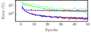
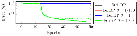
Figure 1: Training progress for 784-256-128-64-10 ReLU MLP trained on MNIST. (Left) Uniform Glorot weight initialization, (right) Negative weight initialization. Solid curves correspond to training errors (in %) and dashed ones are test errors.

In this work we show that several apparently unrelated inference learning methods can be unified via the framework of contrastive surrogates for deeply nested optimization problems. By applying Prop. 2 successively on each level we obtain the following corollary as one consequence of this framework:

Corollary 2.

Let $\ell$ be differentiable and $E_{k}$, $k=1,\dotsc,L$, satisfy the assumptions in Prop. 2, then we have

$$\tfrac{d}{d\theta}\mathcal{L}_{\mathrm{deep}}(\theta) =\tfrac{\partial}{\partial\theta}\lim_{\bm{\beta}\to\mathbf{0}^{+}}\mathcal{L}_{GC}^{\bm{\beta}}(\theta)=\tfrac{\partial}{\partial\theta}\lim_{\bm{\beta}\to\mathbf{0}^{+}}\mathcal{L}_{LC}^{\bm{\beta}}(\theta)=\tfrac{\partial}{\partial\theta}\lim_{\bm{\beta}\to\mathbf{0}^{+}}\bar{}\mathcal{L}_{LC}^{\bm{\beta}}(\theta).$$ (54)

Thus, the methods discussed in Sections 3 and 4.2 are equivalent to standard back-propagation in their respective limit case (and approximate back-propagation for sufficiently small values $\beta_{k}>0$). Hence, constructive arguments specific to a proposed method (such as the ones given in [39, 40]) are not strictly necessary. Additionally it follows, that back-propagation can be extended to rely solely on one-sided directional derivatives instead of regular (strong) derivatives of the activation function.

We conclude by pointing out that in practice the contrastive surrogates are valid objectives to train a DNN in their own right. While the analysis conducted in this paper is largely addressing the limit case $\beta_{k}\to 0^{+}$, when all the discussed methods converge essentially to back-propagation, even finite values for $\beta_{k}>0$ lead to valid learning losses. This is due to $\mathcal{L}^{\bm{\beta}}_{GC}$, $\mathcal{L}_{LC}^{\bm{\beta}}$ and $\bar{}\mathcal{L}_{LC}^{\bm{\beta}}$ attaining the minimal possible objective value only for a perfect predictor (leading also to a minimal target loss $\ell$). Empirical results of existing inference learning methods are given in the respective literature. At this point we illustrate the numerical behavior of Fenchel BP in Fig. 1 for a 4-layer multi-layer perceptron (MLP) trained on MNIST using ADAM [16] as stochastic optimization method (batch size 50, learning rate $0.001$, uniform Glorot or negative weight initialization). The training error (solid lines) and the test error (dashed lines) are depicted using standard and Fenchel back-propagation with different fixed values for $\beta_{k}=\beta\in\{0.01,1,1000\}$ for all $k$. It can be seen in Fig. 1(left), that Fenchel BP for small but non-vanishing choices of $\beta$ reduces the training error similarly well as standard back-propagation, and progress is slowed down only for a large value of $\beta=1000$. On the other hand, a value of $\beta\gg 0$ is able to escape the vanishing gradient problem (Fig. 1(right)). In particular, an all-negative weights initialization for the same ReLU-based MLP—which will not progress using back-propagation due to vanishing gradients—can be successfully trained by Fenchel BP using a sufficiently large value for $\beta$ (achieving 1.7%/2.79% training and test error compared to 88.66%/88.65% for standard BP and Fenchel BP with $\beta\in\{0.01,1\}$). Understanding and exploring this property and other variations of Fenchel BP is subject of future work.

Acknowledgements

We are grateful to Guillaume Bourmaud and to anonymous reviewers for helpful feedback. This work was partially supported by the Wallenberg AI, Autonomous Systems and Software Program (WASP) funded by the Knut and Alice Wallenberg Foundation.

Appendix A Proofs

Proof of Prop. 1.

In the differentiable setting $\hat{z}(\beta)$ satisfies

$$0 =\beta\ell(\hat{z}(\beta)+\frac{\partial E(\hat{z}(\beta);\theta)}{\partial z}$$ (55)

and total differentiation w.r.t. $\beta$ at 0 yields

$$0 =\ell^{\prime}(\hat{z}(\beta))+\frac{\partial^{2}E(\hat{z}(\beta);\theta)}{\partial z^{2}}\frac{d\hat{z}(\beta)}{d\beta}\iff\frac{d\hat{z}(\beta)}{d\beta}=-\left(\frac{\partial^{2}E(\hat{z}(\beta);\theta)}{\partial z^{2}}\right)^{-1}\ell^{\prime}(\hat{z}(\beta))$$ (56)

Letting $\beta\to 0$ and using that $\hat{z}(0)=z^{*}$ yields the claimed relation,

$$\frac{d\hat{z}(\beta)}{d\beta}\big{|}_{\beta=0}=-\!\left(\frac{\partial^{2}E(z^{*};\theta)}{\partial z^{2}}\right)^{-1}\ell^{\prime}(z^{*}).$$ (57)

The second relation in Prop. 1 is obtained by applying the chain rule. ∎

Proof of Prop. 2.

We restate Eq. 14 after introducing slack variables $s\geq 0$

$$E(z;\theta)=f(z;\theta)\qquad\text{s.t. }g_{i}(z)-s_{i}=0\qquad\forall i\notin\mathcal{W}^{*}:s_{i}=0.$$ (58)

The slack variables corresponding to strongly active constraints are forced to 0. Now $\hat{z}(\beta)$ satisfies (where we simply write $\hat{z}$ instead of $\hat{z}(\beta)$)

$$\beta\ell^{\prime}(\hat{z})+f^{\prime}(\hat{z})+\sum\nolimits_{i}\lambda_{i}g_{i}^{\prime}(\hat{z})=0,$$ (59)

where $\lambda_{i}\in\mathbb{R}$ is the Lagrange multipliers for $g_{i}(z)-s_{i}$, and $\ell^{\prime}$, $f^{\prime}$ and $g_{i}^{\prime}$ are derivatives w.r.t. $z$. Taking the total derivative w.r.t. $\beta$ yields

$$\ell^{\prime}(\hat{z})+\beta\ell^{\prime\prime}(\hat{z})\dot{z}+f^{\prime\prime}(\hat{z})\dot{z}+\sum\nolimits_{i}\lambda_{i}^{\top}g_{i}^{\prime\prime}(\hat{z})\dot{z}+g^{\prime}(\hat{z})^{\top}\dot{\lambda}=0,$$ (60)

where $\dot{z}$ and $\dot{\lambda}$ are shorthand notations for $d\hat{z}/d\beta$ and $d\lambda/d\beta$. We introduce

$$\mathtt{A}:=f^{\prime\prime}(z^{*})+\sum\nolimits_{i}\lambda_{i}^{\top}g_{i}^{\prime\prime}(z^{*}) \mathtt{B}:=g^{\prime}(z^{*}).$$ (61)

Thus, the above reads for $\beta\to 0^{+}$:

$$\ell^{\prime}(z^{*})+\mathtt{A}\dot{z}+\mathtt{B}^{\top}\dot{\lambda}=0,$$ (62)

Taking the derivative of the constraint $g(z)-s=0$ yields $\mathtt{B}\dot{z}=\dot{s}$. If the $i$-th constraint is an equality constraint, then $s_{i}$ is constant 0 and therefore $\dot{s}_{i}=0$. Otherwise $\dot{s}_{i}\geq 0$. Overall, we have a linear system of equations,

$$\begin{pmatrix}\mathtt{A}&\mathtt{B}^{\top}\\ \mathtt{B}&\mathtt{0}\end{pmatrix}\binom{\dot{z}}{\dot{\lambda}}=\binom{-\ell^{\prime}}{\dot{s}}.$$ (63)

This system together with $\dot{s}\geq 0$ corresponds to the KKT conditions of the following quadratic program,

$$\tfrac{1}{2}\dot{z}^{\top}{\mathtt{A}}\dot{z}+\mathbf{c}^{\top}\dot{z}\qquad\text{s.t. }{\mathtt{B}}\dot{z}=\dot{s}\qquad\dot{s}\geq 0\qquad\forall i\notin\mathcal{W}^{*}:\dot{s}_{i}=0,$$ (64)

which is equivalent to Eq. 17. ∎

Proof of Prop. 3.

Recall that

$$\mathcal{L}^{\beta}(\theta)=\min_{z}\ell(z)+\tfrac{1}{\beta}\big{(}E(z;\theta)-E(z^{*};\theta)\big{)}=\ell(\hat{z}_{\beta})+\tfrac{1}{\beta}\big{(}E(\hat{z}_{\beta};\theta)-E(z^{*};\theta)\big{)}.$$ (65)

By using the optimality of $\hat{z}_{\beta}$, in particular $\ell(\hat{z}_{\beta})+\beta^{-1}E(\hat{z}_{\beta};\theta)\leq\ell(z)+\beta^{-1}E(z)$ for all $z$, we obtain:

$$\ell(\hat{z}_{\beta})+\beta^{-1}E(\hat{z}_{\beta};\theta)\leq\ell(z^{*})+\beta^{-1}E(z^{*}) \iff\underbrace{\ell(\hat{z}_{\beta})+\beta^{-1}\big{(}E(\hat{z}_{\beta};\theta)-E(z^{*};\theta)\big{)}}_{=\,\mathcal{L}^{\beta}(\theta)}\leq\underbrace{\ell(z^{*})}_{=\,\mathcal{L}(\theta)}$$ (66)

$$\iff\mathcal{L}^{\beta}(\theta)\leq\mathcal{L}(\theta),$$ (67)

which shows the lower bound. Now let $E(z;\theta)$ be strongly convex in $z$ for all $\theta$ with parameter $\nu>0$. Thus,

$$E(z;\theta)\geq E(z^{\prime};\theta)+\nabla_{z}E(z^{\prime};\theta)^{\top}(z-z^{\prime})+\tfrac{\nu}{2}\lVert z-z^{\prime}\rVert^{2}\implies E(z;\theta)\geq E(z^{*};\theta)+\tfrac{\nu}{2}\lVert z-z^{*}\rVert^{2},$$ (68)

and therefore

$$\min_{z}\left\{\ell(z)-\ell(z^{*})+\beta^{-1}E(z;\theta)\right\} \geq\min_{z}\left\{\ell^{\prime}(z^{*})^{\top}(z-z^{*})+\tfrac{1}{\beta}E(z;\theta)\right\}$$ (69)

$$\geq\min_{z}\left\{\ell^{\prime}(z^{*})^{\top}(z-z^{*})+\tfrac{1}{\beta}E(z^{*};\theta)+\tfrac{\nu}{2\beta}\lVert z-z^{*}\rVert^{2}\right\}$$ (70)

$$=\tfrac{1}{\beta}E(z^{*})-\tfrac{\beta}{2\nu}\lVert\ell^{\prime}(z^{*})\rVert^{2},$$ (71)

where the first inequality uses the convexity of $\ell$ and the second one appies the strong convexity of $E$. The last line is obtained by closed form minimization over $z$. Rearranging the above yields

$$\ell(z^{*})\leq\ell(\hat{z})+\tfrac{1}{\beta}\big{(}E(\hat{z};\theta)-E(z^{*};\theta)\big{)}+\tfrac{\beta}{2\nu}\lVert\ell^{\prime}(z^{*})\rVert^{2},$$ (72)

Combining this with the lower bound finally provides

$$\ell(\hat{z})+\tfrac{1}{\beta}\big{(}E(\hat{z};\theta)-E(z^{*};\theta)\big{)}\leq\ell(z^{*})\leq\ell(\hat{z})+\tfrac{1}{\beta}\big{(}E(\hat{z};\theta)-E(z^{*};\theta)\big{)}+\tfrac{\beta}{2\nu}\lVert\ell^{\prime}(z^{*})\rVert^{2},$$ (73)

i.e. Eq. 20. ∎

Proof of Prop. 4.

We start at the innermost level and obtain

$$\min_{\theta}\ell(z_{L}^{*})\qquad\text{s.t. } z_{k}^{*}=\arg\min_{z_{k}}E_{k}(z_{k};z_{k-1}^{*};\theta)\qquad k=3,\dotsc,L$$

$$z_{2}^{*}=\arg\min_{z_{2}}\left\{\min_{z_{1}}\big{\{}E_{2}(z_{2},z_{1};\theta)+\tfrac{1}{\beta_{1}}E_{1}(z_{1};\theta)\big{\}}-\min_{z_{1}}\tfrac{1}{\beta_{1}}E_{1}(z_{1};\theta)\right\}.$$ (74)

We define $\check{E}_{1}(\theta):=\min_{z_{1}}E_{1}(z_{1};\theta)/\beta_{1}$. Hence the above reduces to

$$\min_{\theta}\ell(z_{L}^{*})\qquad\text{s.t. } z_{k}^{*}=\arg\min_{z_{k}}E_{k}(z_{k};z_{k-1}^{*};\theta)\qquad k=3,\dotsc,L$$

$$z_{2}^{*}=\arg\min_{z_{2}}\left\{\min_{z_{1}}\big{\{}E_{2}(z_{2},z_{1};\theta)+\tfrac{1}{\beta_{1}}E_{1}(z_{1};\theta)\big{\}}-\check{E}_{1}(\theta)\right\}.$$ (75)

Applying the expansion on $z_{3}^{*}$ yields

$$\min_{\theta}\ell(z_{L}^{*})\qquad\text{s.t. } z_{k}^{*}=\arg\min_{z_{k}}E_{k}(z_{k};z_{k-1}^{*};\theta)\qquad k=4,\dotsc,L$$

$$z_{3}^{*}=\arg\min_{z_{3}}\bigg{\{}\min_{z_{2}}\left\{E_{3}(z_{3},z_{2};\theta)+\tfrac{1}{\beta_{2}}\min_{z_{1}}\big{\{}E_{2}(z_{2},z_{1};\theta)+\tfrac{1}{\beta_{1}}E_{1}(z_{1};\theta)\big{\}}-\check{E}_{1}(\theta)\right\}$$

$$\hskip 54.00009pt-\tfrac{1}{\beta_{2}}\min_{z_{1},z_{2}}\big{\{}E_{2}(z_{2},z_{1};\theta)+\tfrac{1}{\beta_{1}}E_{1}(z_{1};\theta)-\check{E}_{1}(\theta)\big{\}}\bigg{\}}.$$ (76)

The $\check{E}_{1}(\theta)$ terms cancel, leaving us with

$$\min_{\theta}\ell(z_{L}^{*})\qquad\text{s.t. } z_{k}^{*}=\arg\min_{z_{k}}E_{k}(z_{k};z_{k-1}^{*};\theta)\qquad k=4,\dotsc,L$$

$$z_{3}^{*}=\arg\min_{z_{3}}\bigg{\{}\min_{z_{1},z_{2}}\left\{E_{3}(z_{3},z_{2};\theta)+\tfrac{1}{\beta_{2}}E_{2}(z_{2},z_{1};\theta)+\tfrac{1}{\beta_{1}\beta_{2}}E_{1}(z_{1};\theta)\right\}$$

$$\hskip 54.00009pt-\min_{z_{1},z_{2}}\big{\{}\tfrac{1}{\beta_{2}}E_{2}(z_{2},z_{1};\theta)+\tfrac{1}{\beta_{1}\beta_{2}}E_{1}(z_{1};\theta)\big{\}}\bigg{\}}.$$ (77)

We define

$$U_{2}(\theta):=\min_{z_{1},z_{2}}\big{\{}\tfrac{1}{\beta_{2}}E_{2}(z_{2},z_{1};\theta)+\tfrac{1}{\beta_{1}\beta_{2}}E_{1}(z_{1};\theta)\big{\}}$$ (78)

and generally

$$U_{k}(\theta):=\min_{z_{1},\dotsc,z_{k}}\left\{\sum_{l=1}^{k}\frac{1}{\prod_{j=l}^{k}\beta_{j}}E_{k}(z_{k},z_{k-1};\theta)\right\}.$$ (79)

Thus, we obtain

$$\min_{\theta}\ell(z_{L}^{*})\qquad\text{s.t. } z_{k}^{*}=\arg\min_{z_{k}}E_{k}(z_{k};z_{k-1}^{*};\theta)\qquad k=4,\dotsc,L$$

$$z_{3}^{*}=\arg\min_{z_{3}}\left\{\min_{z_{1},z_{2}}\left\{E_{3}(z_{3},z_{2};\theta)+\tfrac{1}{\beta_{2}}E_{2}(z_{2},z_{1};\theta)+\tfrac{1}{\beta_{1}\beta_{2}}E_{1}(z_{1};\theta)\right\}-U_{2}(\theta)\right\}.$$ (80)

Expanding until $z_{L-1}^{*}$ yields

$$\min_{\theta}\ell(z_{L}^{*})\qquad\text{s.t. }z_{L}^{*}=\arg\min_{z_{L}}\left\{\min_{z_{1},\dotsc,z_{L-1}}\left\{\sum_{k=1}^{L}\frac{1}{\prod_{l=k}^{L-1}\beta_{l}}E_{k}(z_{k},z_{k-1};\theta)\right\}-U_{L-1}(\theta)\right\}$$ (81)

A final expansion step finally results in

$$\min_{\theta}\left\{\min_{z_{1},\dotsc,z_{L}}\left\{\ell(z_{L})+\sum_{k=1}^{L}\frac{E_{k}(z_{k},z_{k-1};\theta)}{\prod_{l=k}^{L-1}\beta_{l}}\right\}-\min_{z_{1},\dotsc,z_{L}}\left\{\sum_{k=1}^{L}\frac{E_{k}(z_{k},z_{k-1};\theta)}{\prod_{l=k}^{L-1}\beta_{l}}\right\}\right\}=\min_{\theta}\,\mathcal{L}_{GC}^{\bm{\beta}}(\theta),$$ (82)

since the $U_{L-1}(\theta)$ terms cancel again. ∎

Proof of Prop. 5.

We start at the outermost level $L$ and obtain

$$\min_{\theta}\left(\min_{z_{L}}\big{\{}\ell(z_{L})+\tfrac{1}{\beta_{L}}E_{L}(z_{L},z_{L-1}^{*};\theta)\big{\}}-\min_{z_{L}}\tfrac{1}{\beta_{L}}E_{L}(z_{L},z_{L-1}^{*};\theta)\right)$$ (83)

subject to $z_{k}^{*}=\arg\min_{z_{k}}E_{k}(z_{k},z_{k-1}^{*};\theta)$ for $k=1,\dotsc,L-1$. Using $z_{L}^{*}=f_{L}(z_{k-1}^{*};\theta)$ and

$$E_{L}(z_{L}^{*},z_{L-1}^{*};\theta)=E_{L}(f_{L}(z_{L-1}^{*};\theta),z_{L-1}^{*};\theta)=:\check{E}_{L}(z_{L-1}^{*};\theta)$$ (84)

the above objective reduces to

$$\min_{\theta} \left(\min_{z_{L}}\big{\{}\ell(z_{L})+\tfrac{1}{\beta_{L}}E_{L}(z_{L},z_{L-1}^{*};\theta)\big{\}}-\tfrac{1}{\beta_{L}}\check{E}_{L}(z_{L-1}^{*};\theta)\right)$$

$$=\min_{\theta} \min_{z_{L}}\big{\{}\ell(z_{L})+\tfrac{1}{\beta_{L}}\big{(}E_{L}(z_{L},z_{L-1}^{*};\theta)-\check{E}_{L}(z_{L-1}^{*};\theta)\big{)}\big{\}}$$ (85)

subject to $z_{k}^{*}=\arg\min_{z_{k}}E_{k}(z_{k},z_{k-1}^{*};\theta)$ for $k=1,\dotsc,L-1$. We have a nested minimization with $L-1$ levels and a modified main objective. We apply the conversion a second time and obtain

$$\min_{\theta} \bigg{(}\min_{z_{L-1}}\left\{\min_{z_{L}}\left\{\ell(z_{L})+\tfrac{1}{\beta_{L}}\big{(}E_{L}(z_{L},z_{L-1};\theta)-\check{E}_{L}(z_{L-1};\theta)\big{)}\right\}+\tfrac{1}{\beta_{L-1}}E_{L-1}(z_{L-1},z_{L-2}^{*};\theta)\right\}$$

$$-\min_{z_{L-1}}\tfrac{1}{\beta_{L-1}}E_{L-1}(z_{L-1},z_{L-2}^{*};\theta)\bigg{)}$$ (86)

$$=\min_{\theta} \min_{z_{L-1},z_{L}}\left\{\ell(z_{L})+\tfrac{1}{\beta_{L}}\big{(}E_{L}(z_{L},z_{L-1};\theta)-\check{E}_{L}(z_{L-1};\theta)\big{)}+\tfrac{1}{\beta_{L-1}}\big{(}E_{L-1}(z_{L-1},z_{L-2}^{*};\theta)-\check{E}_{L-1}(z_{L-2}^{*};\theta)\big{)}\right\}$$ (87)

subject to the constraints on $z_{k}^{*}$ for $k=1,\dotsc,L-2$. By continuing this process we finally arrive at

$$\min_{\theta}\min_{z_{1},\dotsc,z_{L}}\left\{\ell(z_{L})+\sum\nolimits_{k=1}^{L}\frac{1}{\beta_{k}}\big{(}E_{k}(z_{k},z_{k-1};\theta)-\check{E}_{k}(z_{k-1};\theta)\big{)}\right\}$$ (88)

as claimed in the proposition. ∎

Prop. 6.

We introduce $g(z):=\min_{y}h(y,z)$ and $y^{*}(z)=\arg\min_{y}h(y,z)$, and observe that

$$\frac{dg(z)}{dz}=\frac{\partial h(y^{*}(z),z)}{\partial z}+\frac{\partial h(y^{*}(z),z)}{\partial y}\cdot\frac{dy^{*}(z)}{dz}=\frac{\partial h(y^{*}(z),z)}{\partial z},$$ (89)

since $\partial_{y}h(y^{*}(z),z)=0$ by construction. This together with the definition of the linearized surrogate (Eq. 37) yields the result. ∎

Proof of Prop. 7.

For brevity we omit the explicit dependence of $E$ on $\theta$ below. Applying the linearized contrastive surrogate on the outermost level of the deeply nested program in Eq. 21 yields

$$\min_{z_{L}}\left\{\ell(z_{L}^{*})+(z_{L}-z_{L}^{*})^{\top}\ell^{\prime}(z_{L}^{*})+\tfrac{1}{\beta_{L}}E_{L}(z_{L},z_{L-1}^{*})\right\}-\min_{z_{L}}\tfrac{1}{\beta_{L}}E_{L}(z_{L},z_{L-1}^{*})\qquad\text{s.t. }z_{k}^{*}=\arg\min_{z_{k}}E_{k}(z_{k},z_{k-1})$$ (90)

for $k=1,\dotsc,L-1$, where $\ell^{\prime}(z_{L})=\tfrac{d}{dz_{L}}\ell(z_{L})$. Now we apply Prop. 6 with

$$g_{L}^{+}(z_{L-1}) :=\min_{z_{L}}\left\{\ell(z_{L}^{*})+(z_{L}-z_{L}^{*})^{\top}\ell^{\prime}(z_{L}^{*})+\tfrac{1}{\beta_{L}}E_{L}(z_{L},z_{L-1})\right\} g_{L}^{-}(z_{L-1}) :=\min_{z_{L}}\tfrac{1}{\beta_{L}}E_{L}(z_{L},z_{L-1})$$ (91)

and therefore

$$\tfrac{\partial}{\partial z_{L-1}}g_{L}^{+}(z_{L-1})=\tfrac{1}{\beta_{L}}\tfrac{\partial}{\partial z_{L-1}}E_{L}(\bar{z}_{L},z_{L-1}) \tfrac{\partial}{\partial z_{L-1}}g_{L}^{-}(z_{L-1})=\tfrac{1}{\beta_{L}}\tfrac{\partial}{\partial z_{L-1}}E_{L}(z_{L}^{*},z_{L-1}),$$ (92)

where $\bar{z}_{L}$ and $z_{L}^{*}$ are the respective minimizers,

$$\bar{z}_{L}:=\min_{z_{L}}\left\{\ell(z_{L}^{*})+(z_{L}-z_{L}^{*})^{\top}\ell^{\prime}(z_{L}^{*})+\tfrac{1}{\beta_{L}}E_{L}(z_{L},z_{L-1})\right\} z_{L}^{*}:=\arg\min_{z_{L}}\tfrac{1}{\beta_{L}}E_{L}(z_{L},z_{L-1}).$$ (93)

Hence, the linearization of the outer loss in Eq. 90 at $z_{L-1}^{*}$ is given by

$$z_{L-1} \mapsto\min_{z_{L}}\left\{\ell(z_{L}^{*})+(z_{L}-z_{L}^{*})^{\top}\ell^{\prime}(z_{L}^{*})+\tfrac{1}{\beta_{L}}E_{L}(z_{L},z_{L-1}^{*})\right\}-\min_{z_{L}}\tfrac{1}{\beta_{L}}E_{L}(z_{L},z_{L-1}^{*})$$

$$+(z_{L-1}-z_{L-1}^{*})^{\top}\tfrac{1}{\beta_{L}}\tfrac{\partial}{\partial z_{L-1}}\big{(}E_{L}(\bar{z}_{L},z_{L-1}^{*})-E_{L}(z_{L}^{*},z_{L-1}^{*})\big{)}$$ (94)

$$=\ell(z_{L}^{*})+(\bar{z}_{L}-z_{L}^{*})^{\top}\ell^{\prime}(z_{L}^{*})+\tfrac{1}{\beta_{L}}E_{L}(\bar{z}_{L},z_{L-1}^{*})-\tfrac{1}{\beta_{L}}E_{L}(z_{L}^{*},z_{L-1}^{*})$$

$$+(z_{L-1}-z_{L-1}^{*})^{\top}\tfrac{1}{\beta_{L}}\tfrac{\partial}{\partial z_{L-1}}\big{(}E_{L}(\bar{z}_{L},z_{L-1}^{*})-E_{L}(z_{L}^{*},z_{L-1}^{*})\big{)}$$ (95)

$$=\ell(z_{L}^{*})+(\bar{z}_{L}-z_{L}^{*})^{\top}\ell^{\prime}(z_{L}^{*})+\tfrac{1}{\beta_{L}}h_{L}(\bar{z}_{L},z_{L-1}^{*})+(z_{L-1}-z_{L-1}^{*})^{\top}\tfrac{1}{\beta_{L}}\tfrac{\partial}{\partial z_{L-1}}h_{L}(\bar{z}_{L},z_{L-1}^{*})$$ (96)

using $h_{k}(z_{k},z_{k-1}):=E_{k}(z_{k},z_{k-1})-\min_{z_{k}^{\prime}}E_{k}(z_{k}^{\prime},z_{k-1})$. Thus, after the second step of applying the linearized contrastive surrogates we arrive at

$$\ell(z_{L}^{*})+(\bar{z}_{L}-z_{L}^{*})^{\top}\ell^{\prime}(z_{L}^{*})+\tfrac{1}{\beta_{L}}h_{L}(\bar{z}_{L},z_{L-1}^{*})$$

$$+\min_{z_{L-1}}\left\{(z_{L-1}-z_{L-1}^{*})^{\top}\tfrac{1}{\beta_{L}}\tfrac{\partial}{\partial z_{L-1}}h_{L}(\bar{z}_{L},z_{L-1}^{*})+\tfrac{1}{\beta_{L-1}}E_{L-1}(z_{L-1},z_{L-2}^{*})\right\}-\min_{z_{L-1}}\tfrac{1}{\beta_{L-1}}E_{L-1}(z_{L-1},z_{L-2}^{*})$$ (97)

$$=\ell(z_{L}^{*})+(\bar{z}_{L}-z_{L}^{*})^{\top}\ell^{\prime}(z_{L}^{*})+\tfrac{1}{\beta_{L}}h_{L}(\bar{z}_{L},z_{L-1}^{*})+(\bar{z}_{L-1}-z_{L-1}^{*})^{\top}\tfrac{1}{\beta_{L}}\tfrac{\partial}{\partial z_{L-1}}h_{L}(\bar{z}_{L},z_{L-1}^{*})+\tfrac{1}{\beta_{L-1}}h_{L-1}(\bar{z}_{L-1},z_{L-2}^{*})$$ (98)

subject to $z_{k}^{*}=\arg\min_{z_{k}}E_{k}(z_{k},z_{k-1})$ for $k=L-2,\dotsc,1$. Continuation of these steps until the innermost level yields the claim of Prop. 7. ∎

Appendix B Bottom-Up Traversal for Linearized Surrogates

Using the linearized surrogate (Eq. 37) is only possible if $\ell(\cdot)$ is differentiable and each $E_{k}(z_{k},z_{k-1})$ is differentiable in $z_{k-1}$. Recall that $z_{k}^{*}:=\arg\min_{z_{k}}E_{k}(z_{k},z_{k-1})$ (and $z_{1}^{*}=\arg\min_{z_{1}}E_{1}(z_{1};\theta)$). Proceeding analogously to Prop. 4 but using the linearized contrastive surrogates yields a modified global contrastive objective, where the clamped and free energies are suitable linearized versions of $\mathcal{E}^{\bm{\beta}}$ and $\hat{}\mathcal{E}^{\bm{\beta}}$:

Proposition 8.

Let $\bm{\beta}=(\beta_{1},\dotsc,\beta_{L})$ be positive spacing parameters. Applying the linearized contrastive surrogate (Eq. 37) recursively on Eq. 21 from the innermost to the outermost level yields the following linearized global contrastive objective,

$$\bar{}\mathcal{L}^{\bm{\beta}}_{GC}(\theta):=\min_{z_{1},\dotsc,z_{L}}\left\{\ell(z_{L}^{*})+(z_{L}-z_{L}^{*})^{\top}\ell^{\prime}(z_{L}^{*})+\bar{}\mathcal{E}^{\bm{\beta}}(z;\theta)\right\}-\min_{z_{1},\dotsc,z_{L}}\bar{}\mathcal{E}^{\bm{\beta}}(z;\theta),$$ (99)

where

$$\bar{}\mathcal{E}^{\bm{\beta}}(z;\theta):=\sum_{k=2}^{L}\frac{E_{k}(z_{k},z_{k-1}^{*};\theta)+(z_{k-1}-z_{k-1}^{*})^{\top}\partial_{z_{k-1}}E_{k}(z_{k},z_{k-1}^{*};\theta)}{\prod_{l=k}^{L}\beta_{l}}+\frac{E_{1}(z_{1};\theta)}{\prod_{l=1}^{L}\beta_{l}}.$$ (100)

In contrast to the global contrastive objective in Prop. 4, the resulting subproblem $\bar{}\mathcal{E}^{\bm{\beta}}(z;\theta)$ is generally not convex in $z$ even when $\mathcal{E}^{\bm{\beta}}$ is. $z_{k}$ depends on both $z_{k-1}$ and $z_{k+1}$ in $\bar{}\mathcal{E}^{\bm{\beta}}$, hence minimizing $\bar{}\mathcal{E}^{\bm{\beta}}$ (and its loss-augmented variant) poses usually a difficult, non-convex optimization problem in $z_{1},\dotsc,z_{L}$. Consequently, the resulting linearized global contrastive objective $\bar{}\mathcal{L}^{\bm{\beta}}_{GC}$ is of little further interest.

Appendix C Julia Source Code

The plots in Fig. 1 in the main text were obtained by running the Julia code below.

using Statistics, MLDatasets
using Flux, Flux.Optimise
using Flux: onehotbatch, onecold, crossentropy
using Base.Iterators: partition
using ChainRulesCore, Random

train_x, train_y = MNIST.traindata(); test_x, test_y  = MNIST.testdata()

train_X = Float32.(reshape(train_x, 28, 28, 1, :));
test_X = Float32.(reshape(test_x, 28, 28, 1, :));

train_Y = onehotbatch(train_y, 0:9); test_Y  = onehotbatch(test_y, 0:9)

########################################################################

# Configure settings
use_negative_init = false
use_FenBP = true

const beta = 0.01f0

########################################################################

my_relu(x) = relu(x)

function ChainRulesCore.rrule(::typeof(my_relu), x)
    z = my_relu(x)
    function pullback(dy)
        zz = my_relu(x - beta*dy)
        return NoTangent(), (z - zz) / beta
    end
    return z, pullback
end

# We use this definition to prevent Flux from optimizing away our custom AD rule.
function my_act(x; use_FenBP = use_FenBP)
    return use_FenBP ? map(my_relu, x) : relu.(x)
end

########################################################################

glorot_neg_uniform(rng::AbstractRNG, dims...) = (-abs.((rand(rng, Float32, dims...)
                                        .- 0.5f0) .* sqrt(24.0f0 / sum(Flux.nfan(dims...)))))
glorot_neg_uniform(dims...) = glorot_neg_uniform(Random.GLOBAL_RNG, dims...)

########################################################################

# Fix random seed for repeatability across runs
Random.seed!(42)

m = Chain(
    x -> reshape(x, :, size(x, 4)),
    Dense(28*28, 256, init = use_negative_init ? glorot_neg_uniform : Flux.glorot_uniform),
    my_act,
    Dense(256, 128), my_act,
    Dense(128, 64),  my_act,
    Dense(64, 10),   softmax
)

loss(x, y) = sum(crossentropy(m(x), y))
accuracy(x, y) = mean(onecold(m(x), 1:10) .== onecold(y, 1:10))

eta = 0.001f0; opt = ADAM(eta)

train = ([(train_X[:,:,:,i], train_Y[:,i]) for i in partition(1:50000, 50)])

epochs = 50
for epoch = 1:epochs
    iter = 1
    total_loss = 0.f0; train_accuracy = 0.f0

    for d in train
        ps = params(m)
        gs = gradient(ps) do
            l = loss(d...); total_loss += l; train_accuracy += accuracy(d...); l
        end
        update!(opt, ps, gs); iter += 1
    end

    total_loss /= iter; train_accuracy /= iter
    test_accuracy = accuracy(test_X, test_Y)

    println(epoch, " loss: ", total_loss,
            " (approx) train accuracy: ", 100*train_accuracy,
            " test accuracy: ", 100*test_accuracy,
            " (approx) train error: ", 100-100*train_accuracy,
            " test error: ", 100-100*test_accuracy)
end

References

• [1] Luis B Almeida. A learning rule for asynchronous perceptrons with feedback in a combinatorial environment. In Artificial neural networks: concept learning, pages 102–111. 1990.
• [2] Ehsan Amid, Rohan Anil, and Manfred K Warmuth. Locoprop: Enhancing backprop via local loss optimization. arXiv preprint arXiv:2106.06199, 2021.
• [3] Armin Askari, Geoffrey Negiar, Rajiv Sambharya, and Laurent El Ghaoui. Lifted neural networks. arXiv preprint arXiv:1805.01532, 2018.
• [4] Yoshua Bengio. Gradient-based optimization of hyperparameters. Neural computation, 12(8):1889–1900, 2000.
• [5] Yoshua Bengio. How auto-encoders could provide credit assignment in deep networks via target propagation. arXiv preprint arXiv:1407.7906, 2014.
• [6] Yoshua Bengio, Dong-Hyun Lee, Jorg Bornschein, Thomas Mesnard, and Zhouhan Lin. Towards biologically plausible deep learning. arXiv preprint arXiv:1502.04156, 2015.
• [7] Kristin P Bennett, Gautam Kunapuli, Jing Hu, and Jong-Shi Pang. Bilevel optimization and machine learning. In IEEE World Congress on Computational Intelligence, pages 25–47. Springer, 2008. Bilevel optimization to model minimizing test error subject to parameters are minimizing training error.
• [8] Miguel Carreira-Perpinan and Weiran Wang. Distributed optimization of deeply nested systems. In Artificial Intelligence and Statistics, pages 10–19, 2014.
• [9] Stephan Dempe and Alain B Zemkoho. The bilevel programming problem: reformulations, constraint qualifications and optimality conditions. Mathematical Programming, 138(1):447–473, 2013.
• [10] Justin Domke. Generic methods for optimization-based modeling. In Artificial Intelligence and Statistics, pages 318–326. PMLR, 2012.
• [11] Luca Franceschi, Paolo Frasconi, Saverio Salzo, Riccardo Grazzi, and Massimiliano Pontil. Bilevel programming for hyperparameter optimization and meta-learning. In International Conference on Machine Learning, pages 1568–1577. PMLR, 2018. Proves that unrolling converges to correct solution.
• [12] Thomas Frerix, Thomas Möllenhoff, Michael Moeller, and Daniel Cremers. Proximal backpropagation. arXiv preprint arXiv:1706.04638, 2017.
• [13] Stephen Gould, Richard Hartley, and Dylan Campbell. Deep declarative networks: A new hope. arXiv preprint arXiv:1909.04866, 2019.
• [14] Fangda Gu, Armin Askari, and Laurent El Ghaoui. Fenchel lifted networks: A lagrange relaxation of neural network training. arXiv preprint arXiv:1811.08039, 2018.
• [15] Rasmus Kjær Høier and Christopher Zach. Lifted regression/reconstruction networks. In British Machine Vision Conference, 2020.
• [16] Diederik P Kingma and Jimmy Ba. A method for stochastic optimization. In ICLR, 2015.
• [17] Charles D Kolstad and Leon S Lasdon. Derivative evaluation and computational experience with large bilevel mathematical programs. Journal of optimization theory and applications, 65(3):485–499, 1990.
• [18] Karl Kunisch and Thomas Pock. A bilevel optimization approach for parameter learning in variational models. SIAM Journal on Imaging Sciences, 6(2):938–983, 2013.
• [19] Yann LeCun. A theoretical framework for back-propagation. In Proceedings of the 1988 connectionist models summer school, volume 1, pages 21–28, 1988.
• [20] Dong-Hyun Lee, Saizheng Zhang, Asja Fischer, and Yoshua Bengio. Difference target propagation. In Joint european conference on machine learning and knowledge discovery in databases, pages 498–515. Springer, 2015.
• [21] Jia Li, Cong Fang, and Zhouchen Lin. Lifted proximal operator machines. arXiv preprint arXiv:1811.01501, 2018.
• [22] Jonathan Lorraine, Paul Vicol, and David Duvenaud. Optimizing millions of hyperparameters by implicit differentiation. In International Conference on Artificial Intelligence and Statistics, pages 1540–1552. PMLR, 2020.
• [23] Dougal Maclaurin, David Duvenaud, and Ryan Adams. Gradient-based hyperparameter optimization through reversible learning. In International conference on machine learning, pages 2113–2122. PMLR, 2015.
• [24] Julien Mairal, Francis Bach, and Jean Ponce. Task-driven dictionary learning. IEEE transactions on pattern analysis and machine intelligence, 34(4):791–804, 2011.
• [25] Alexander Meulemans, Francesco S Carzaniga, Johan AK Suykens, João Sacramento, and Benjamin F Grewe. A theoretical framework for target propagation. arXiv preprint arXiv:2006.14331, 2020.
• [26] Beren Millidge, Alexander Tschantz, and Christopher L Buckley. Predictive coding approximates backprop along arbitrary computation graphs. arXiv preprint arXiv:2006.04182, 2020.
• [27] Javier R Movellan. Contrastive hebbian learning in the continuous hopfield model. In Connectionist Models, pages 10–17. Elsevier, 1991.
• [28] Peter Ochs, René Ranftl, Thomas Brox, and Thomas Pock. Techniques for gradient-based bilevel optimization with non-smooth lower level problems. Journal of Mathematical Imaging and Vision, 56(2):175–194, 2016.
• [29] Alexander G Ororbia and Ankur Mali. Biologically motivated algorithms for propagating local target representations. In Proceedings of the aaai conference on artificial intelligence, volume 33, pages 4651–4658, 2019.
• [30] Ji$\mathbf{r}$í V Outrata. A note on the usage of nondifferentiable exact penalties in some special optimization problems. Kybernetika, 24(4):251–258, 1988.
• [31] Fernando J Pineda. Generalization of back-propagation to recurrent neural networks. Physical review letters, 59(19):2229, 1987.
• [32] Aravind Rajeswaran, Chelsea Finn, Sham Kakade, and Sergey Levine. Meta-learning with implicit gradients. arXiv preprint arXiv:1909.04630, 2019.
• [33] David E Rumelhart, Geoffrey E Hinton, and Ronald J Williams. Learning representations by back-propagating errors. Nature, 323(6088):533–536, 1986.
• [34] Franco Scarselli, Marco Gori, Ah Chung Tsoi, Markus Hagenbuchner, and Gabriele Monfardini. The graph neural network model. IEEE Transactions on Neural Networks, 20(1):61–80, 2008.
• [35] Benjamin Scellier and Yoshua Bengio. Equilibrium propagation: Bridging the gap between energy-based models and backpropagation. Frontiers in computational neuroscience, 11:24, 2017.
• [36] Yuhang Song, Thomas Lukasiewicz, Zhenghua Xu, and Rafal Bogacz. Can the brain do backpropagation?—exact implementation of backpropagation in predictive coding networks. NeuRIPS Proceedings 2020, 33(2020), 2020.
• [37] Paul J Werbos. Backpropagation through time: what it does and how to do it. Proceedings of the IEEE, 78(10):1550–1560, 1990.
• [38] James CR Whittington and Rafal Bogacz. An approximation of the error backpropagation algorithm in a predictive coding network with local hebbian synaptic plasticity. Neural computation, 29(5):1229–1262, 2017.
• [39] Xiaohui Xie and H Sebastian Seung. Equivalence of backpropagation and contrastive hebbian learning in a layered network. Neural computation, 15(2):441–454, 2003.
• [40] Christopher Zach and Virginia Estellers. Contrastive learning for lifted networks. In British Machine Vision Conference, 2019.
• [41] Christopher Zach and Huu Le. Truncated inference for latent variable optimization problems. In Proc. ECCV, 2020.
• [42] Ziming Zhang and Matthew Brand. Convergent block coordinate descent for training tikhonov regularized deep neural networks. In Advances in Neural Information Processing Systems, pages 1721–1730, 2017.
• [43] Pan Zhou, Chao Zhang, and Zhouchen Lin. Bilevel model-based discriminative dictionary learning for recognition. IEEE transactions on image processing, 26(3):1173–1187, 2016. Supervised dictionary learning using KKT conditions.