First direct neutrino-mass measurement with sub-eV sensitivity

Abstract

We report the results of the second measurement campaign of the Karlsruhe Tritium Neutrino (KATRIN) experiment. KATRIN probes the effective electron anti-neutrino mass, $m_{\nu}$, via a high-precision measurement of the tritium $\upbeta$-decay spectrum close to its endpoint at $18.6\text{\,}\mathrm{keV}$. In the second physics run presented here, the source activity was increased by a factor of 3.8 and the background was reduced by $25\,\%$ with respect to the first campaign. A sensitivity on $m_{\nu}$  of $0.7\text{\,}\mathrm{eV}\mathrm{/}\mathrm{c}\mathrm{{}^{2}}$ at $90\text{\,}\mathrm{\char 37\relax}$ confidence level (CL) was reached. This is the first sub-eV sensitivity from a direct neutrino-mass experiment. The best fit to the spectral data yields $\mbox{$m_{\nu}^{2}$}=$0.26\pm 0.34\text{\,}\mathrm{eV}\mathrm{{}^{2}}\mathrm{/}\mathrm{c}^{4}$$, resulting in an upper limit of $m_{\nu}<$0.9\text{\,}\mathrm{eV}\mathrm{/}\mathrm{c}\mathrm{{}^{2}}$$ ($90\text{\,}\mathrm{\char 37\relax}$ CL). By combining this result with the first neutrino mass campaign, we find an upper limit of $\mbox{$m_{\nu}$}<$0.8\text{\,}\mathrm{eV}\mathrm{/}\mathrm{c}\mathrm{{}^{2}}$$ ($90\text{\,}\mathrm{\char 37\relax}$ CL).

I Introduction

The discovery of neutrino flavour oscillations [1, 2] proves that neutrinos must have a mass, unlike originally assumed in the Standard Model (SM) of Particle Physics. Neutrino oscillation experiments have shown that the weakly interacting neutrino flavour eigenstates, $\nu_{f}$ with $f\in\{\text{e},\upmu,\uptau\}$, are admixtures of the three neutrino mass eigenstates $\nu_{i}$ with mass eigenvalues $m_{i}$. While neutrino-oscillation experiments can probe the differences of squared neutrino mass eigenvalues $\Delta m_{ij}^{2}$, the absolute neutrino-mass scale remains one of the most pressing open questions in the fields of nuclear, particle, and astroparticle physics today. In this paper we report a measurement of the effective electron anti-neutrino mass defined as $\mbox{$m_{\nu}^{2}$}=\sum_{i}|U_{\mathrm{e}i}|^{2}m_{i}^{2}$ where $U_{\mathrm{e}i}$ are elements of the Pontecorvo-Maki-Nakagawa-Sakata (PMNS) matrix, which describes the mixing of the neutrino states.

The neutrino masses are at least five orders of magnitude smaller than the mass of any other fermion of the SM, which may point to a different underlying mass-creation mechanism [3]. The determination of the neutrino mass would thus shed light on the fundamental open question of the origin of particle masses. Despite the smallness of their masses, neutrinos play a crucial role in the evolution of large-scale structures of our cosmos due to their high abundance in the universe [4, 5]. A direct measurement of the neutrino mass could hence provide a key input to cosmological structure-formation models. In this respect, cosmological observations themselves provide stringent limits on the sum of neutrino masses of $\sum m_{i}<$0.12\text{\,}\mathrm{eV}$$ ($95\text{\,}\mathrm{\char 37\relax}$ CL) [6, 7]. However, these limits strongly rely on the underlying cosmological assumptions [8, 9]. An independent measurement of the neutrino mass could help to break parameter degeneracies of the cosmological models. A powerful way to probe this neutrino property in the laboratory is via a search for neutrinoless double $\upbeta$-decay, providing limits at the level of $m_{\upbeta\upbeta}<$0.08\text{\,}\mathrm{-}$$0.18\text{\,}\mathrm{eV}$$ ($90\text{\,}\mathrm{\char 37\relax}$ CL) [10, 11], depending on the nuclear matrix element calculation. In contrast to $m_{\nu}$, the effective mass in double-beta decay is given by $m_{\upbeta\upbeta}=\left|\sum_{i}U_{\mathrm{e}i}^{2}m_{i}\right|$. The limit is only valid under the assumption that neutrinos are their own anti-particle (Majorana particle) and that light neutrinos mediate the decay.

The most direct way to assess the neutrino mass is via the kinematics of a single $\upbeta$-decay. This method is independent of any cosmological model and of the mass nature of the neutrino, i.e. it may be a lepton of Majorana or Dirac type. The neutrino masses $m_{\mathrm{i}}$ lead to a reduction of the maximal observed energy of the decay and a small spectral shape distortion close to the kinematic endpoint of the $\upbeta$-spectrum. In the quasi-degenerate mass regime, where $m_{i}>$0.2\text{\,}\mathrm{eV}$$, the mass splittings are negligible with respect to the masses, $m_{i}$, and the observable can be approximated as $\mbox{$m_{\nu}^{2}$}=\sum_{i}|U_{\mathrm{e}i}|^{2}m_{i}^{2}$.

The Karlsruhe Tritium Neutrino (KATRIN) experiment [12, 13] exploits the single $\upbeta$-decay of molecular tritium

$$\ce{T2}\to\ce{{}^{3}HeT+}+\mathrm{e}^{-}+\bar{\nu}_{e}$$ (1)

and currently provides the best neutrino mass sensitivity in the field of direct neutrino-mass measurements with its first published limit of $\mbox{$m_{\nu}$}<$1.1\text{\,}\mathrm{eV}$$ ($90\text{\,}\mathrm{\char 37\relax}$ CL) [14, 15]. KATRIN is designed to determine the neutrino mass with a sensitivity of close to $0.2\text{\,}\mathrm{eV}$ ($90\text{\,}\mathrm{\char 37\relax}$ CL) in a total measurement time of 1000 days [12]. In this work, we present the second neutrino-mass result of KATRIN, reaching an unprecedented sub-eV sensitivity and limit in $m_{\nu}$ from a direct measurement.

II Experimental setup

The design requirements to detect the small signature of a neutrino mass in the last few eV of a $\upbeta$-decay spectrum are: a high tritium activity ($1\text{\times}{10}^{11}\text{\,}\mathrm{Bq}$), a low background rate ($\lesssim$ 0.1 counts per second (cps)), an eV-scale energy resolution, and an accurate ($0.1\text{\,}\mathrm{\char 37\relax}$-level) theoretical prediction of the integral spectrum.

The KATRIN experiment tackles these challenges by combining a high-activity molecular tritium source with a high-resolution spectrometer of the Magnetic Adiabatic Collimation and Electrostatic (MAC-E)-Filter type [13]. The experiment is hosted by the Tritium Laboratory Karlsruhe (TLK) allowing the safe supply of tritium at the 10-gramme scale with continuous tritium reprocessing [16, 17]. Fig. 1 shows the 70-m long KATRIN beamline.

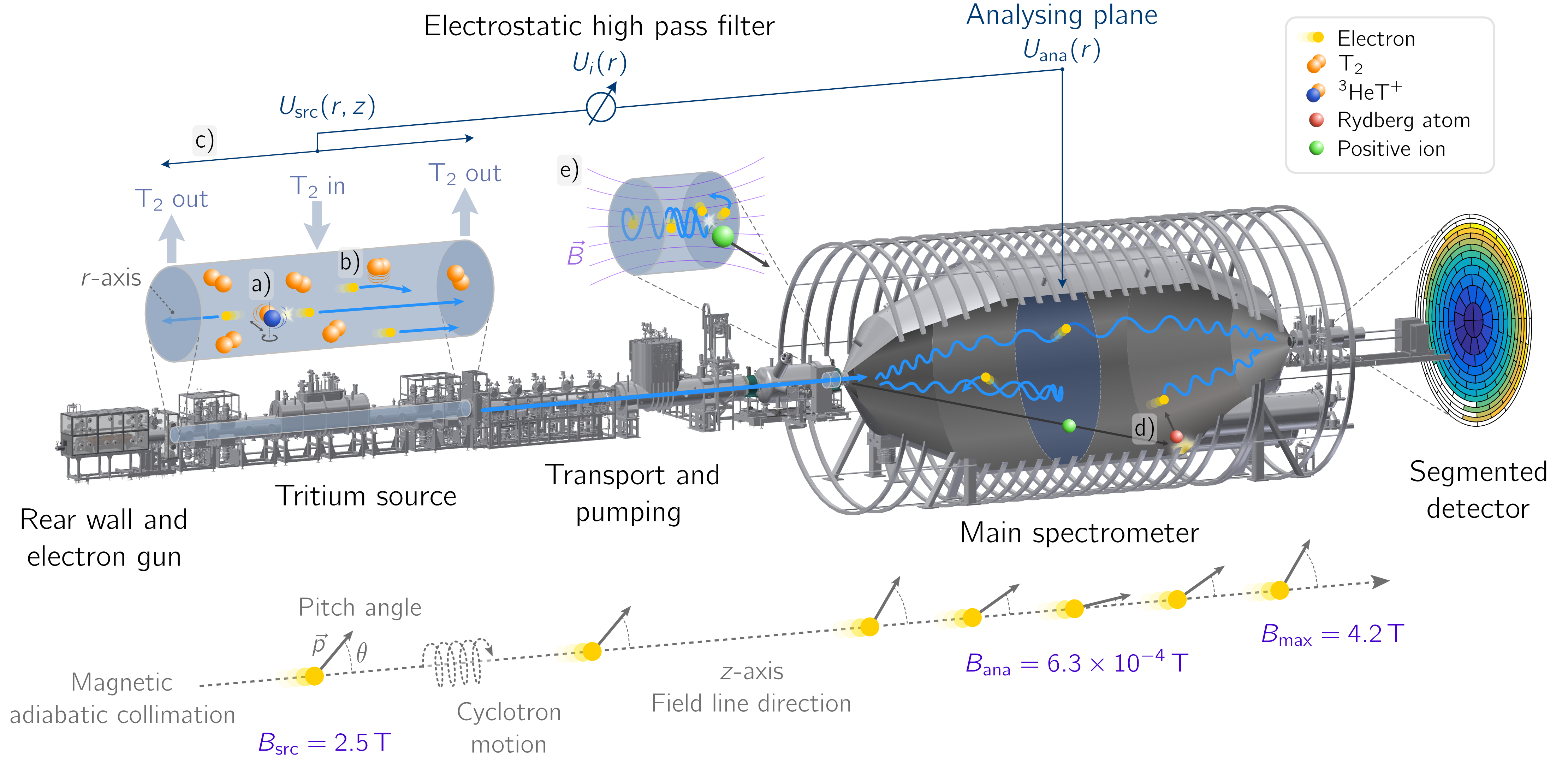
Figure 1: Working principle of the KATRIN experiment as explained in the main text. The view into the tritium source depicts three systematic effects: a) molecular excitations during $\upbeta$-decay, b) scattering of electrons off the gas molecules, and c) spatial distribution of the electric potential in the source $U_{\mathrm{src}}(r,z)$. The view into the spectrometer illustrates the main background processes. Generally, unstable neutral particles (d) can enter the large spectrometer volume and decay. The resulting electrons are accelerated by $qU_{\mathrm{ana}}$ towards the detector, making them indistinguishable from signal electrons [18, 14]. The unstable neutral particles are either ²¹⁹Rn and ²²⁰Rn emanated from the getter pumps [19, 20] or highly excited atoms sputtered off the inner spectrometer surfaces [21, 22, 23]. The sputtering mechanisms originate from both $\alpha$-decays of ²¹⁰Po in the structural material and a Penning trap (e), which gives rise to accelerated positive ions from the volume between the two spectrometers [24]. Note that the white pixels in the detector were excluded from analysis as they do not fulfil the ‘golden pixel’ quality criteria. The magnetic adiabatic collimation is only sketched for the case without electric field for illustration purposes.

The isotope tritium has a short half life of 12.3 years and a low endpoint of $18.6\text{\,}\mathrm{keV}$, both favourable properties to achieve high count rates near the endpoint. Moreover, the theoretical calculation of the super-allowed decay of tritium is well understood [25, 26, 27]. The strong gaseous tritium source (nominal activity $1\text{\times}{10}^{11}\text{\,}\mathrm{Bq}$) is established by the throughput of $40\text{\,}\mathrm{g}$/day of molecular tritium through the 10-m long source tube, which is cooled to $30\text{\,}\mathrm{K}$ to reduce thermal motion of the tritium molecules.

A system of 24 superconducting magnets [28] guides the electrons out of the source towards the spectrometer section and to the detector. Between the source and spectrometer, differential [29] and cryogenic [30] pumping systems reduce the flow of tritium by 14 orders of magnitude.

High-precision electron spectroscopy is achieved with the spectrometer of MAC-E-filter type [31, 32]. The spectrometer acts as a sharp electro-static high-pass filter, transmitting only electrons (of charge $q=-e$) above an adjustable energy threshold $qU$, where $U$ is the retarding potential applied at the spectrometer. A reduction of the magnetic field strength by about four orders of magnitudes from the entrance (exit) of the spectrometer $B_{\mathrm{source}}=$2.5\text{\,}\mathrm{T}$$ ($B_{\mathrm{max}}=$4.2\text{\,}\mathrm{T}$$) to its center, the analysing plane ($B_{\mathrm{ana}}=$6.3\text{\times}{10}^{-4}\text{\,}\mathrm{T}$$), collimates the electron momenta. This configuration creates a narrow filter width of $\Delta E=$18.6\text{\,}\mathrm{keV}$\cdot(B_{\mathrm{ana}}/B_{\mathrm{max}})=$2.8\text{\,}\mathrm{eV}$$ and allows for a large angular acceptance, with a maximum pitch-angle  for the $\upbeta$-decay electrons of $\theta_{\mathrm{max}}=\arcsin{\sqrt{(B_{\mathrm{source}}/B_{\mathrm{max}})}}=50.4^{\circ}$ in the source. A 12-m diameter magnetic coil system surrounding the spectrometer fine-shapes the magnetic field and compensates the Earth’s magnetic field [33, 34].

The transmitted electrons are detected by a 148-pixel silicon PIN-diode focal-plane detector installed at the exit of the spectrometer [35]. By measuring the count rate of transmitted electrons for a set of $qU$ values, the integral $\upbeta$-decay spectrum is obtained. The main spectrometer is preceded by a smaller pre-spectrometer, which operates on the same principle and transmits only electrons above $10\text{\,}\mathrm{keV}$, to reduce the flux of electrons into the main spectrometer. The up-stream end of the beamline is terminated with a gold-plated rear wall, which absorbs the non-transmitted $\upbeta$-electrons and defines the reference electric potential of the source. The rear wall is biased to a voltage ($\mathcal{O}($100\text{\,}\mathrm{mV}$)$) to minimise the difference of its surface potential to that of the beam tube, which minimises the inhomogeneity of the source electric potential.

The rear section is equipped with an angular- and energy-selective electron gun [36], which is used to precisely determine the scattering probability of electrons with the source gas, governed by the product of column density (number of molecules per cm² along the length of the source) and scattering cross section. Furthermore, we use the electron gun to measure the distribution of energy losses for $18.6\text{\,}\mathrm{keV}$ electrons scattering off the molecular tritium gas, providing the most precise energy loss function for this process to date  [37]. Another key calibration source is gaseous krypton, which can be co-circulated with the tritium gas [38]. Mono-energetic conversion electrons from the decay of the meta-stable state ^83mKr are used to determine spatial and temporal variations of the electric potential in the tritium source. The variations are caused by a weak cold-magnetised plasma, which arises from the high magnetic field ($2.5\text{\,}\mathrm{T}$) and a large number of ions and low-energy electrons ($\approx$1\text{\times}{10}^{12}\text{\,}{\mathrm{m}}^{-3}$$) in the tritium source. The methods of calibration are described in more detail in Sec. VII.

The beamline is equipped with multiple monitoring devices. A laser Raman system continuously monitors the gas composition, providing a measurement at the $0.1\text{\,}\mathrm{\char 37\relax}$-precision level each minute. A silicon drift detector system, installed in the transport section, as well as a beta-induced X-ray system at the rear section [39], continuously monitor the tritium activity, obtaining a result at the $0.1\text{\,}\mathrm{\char 37\relax}$-precision level each minute. The high voltage of the main spectrometer is continuously measured at the ppm level with a high-precision voltage divider system [40, 41] and an additional monitoring spectrometer [42]. The magnetic fields are determined with a high-precision magnetic field sensor system [43].

After the successful commissioning of the complete KATRIN beamline in summer 2017 [44], first tritium operation was demonstrated with a small tritium activity of ($5\text{\times}{10}^{8}\text{\,}\mathrm{Bq}$) in mid-2018 [45]. During the first neutrino mass campaign (KNM1) in 2019 [14], the source was operated in a ‘burn-in’ configuration at a reduced activity of $2.5\text{\times}{10}^{10}\text{\,}\mathrm{Bq}$, which is required when structural materials are exposed to high amounts of tritium for the first time. Major technical achievements of the second measurement campaign (KNM2) are the operation of the tritium source at its nominal activity of $9.5\text{\times}{10}^{10}\text{\,}\mathrm{Bq}$ and improved vacuum conditions in the spectrometer [46] that led to a reduction of the background by $25\text{\,}\mathrm{\char 37\relax}$ to $220\text{\,}\mathrm{m}\mathrm{c}\mathrm{p}\mathrm{s}$. We thus increased the $\upbeta$-electron-to-background ratio by a factor of 2.7 with respect to the first campaign. In the last $40\text{\,}\mathrm{eV}$ of the integral spectrum, we collected a total number of $3.7\text{\times}{10}^{6}\text{\,}$ $\upbeta$-electrons. Fig. 2 a) compares the spectra of both neutrino mass campaigns. A direct comparison of the experimental parameters is given in Tab. 1.

Table 1: Comparison of key numbers for KATRIN Neutrino Mass (KNM) campaigns. KNM1 refers to the first KATRIN results [14] and KNM2 to this work. The total number of $\upbeta$-electrons is counted in the last $40\text{\,}\mathrm{eV}$ interval of the integral spectrum, which is used for the spectral fit. The $\upbeta$-electron-to-background ratio is given by the ratio of this number and the background counts in the same energy range, i. e. $E_{0}-$40\text{\,}\mathrm{eV}$$ to $E_{0}$.

	KNM1	KNM2
Number of scans	274	361
Total scan time	$521.7\text{\,}\mathrm{h}$	$743.7\text{\,}\mathrm{h}$
Background rate	$290\text{\,}\mathrm{m}\mathrm{c}\mathrm{p}\mathrm{s}$	$220\text{\,}\mathrm{m}\mathrm{c}\mathrm{p}\mathrm{s}$
T2 column density	$1.11\text{\times}{10}^{17}\text{\,}{\mathrm{cm}}^{-2}$	$4.23\text{\times}{10}^{17}\text{\,}{\mathrm{cm}}^{-2}$
Source activity	$2.5\text{\times}{10}^{10}\text{\,}\mathrm{Bq}$	$9.5\text{\times}{10}^{10}\text{\,}\mathrm{Bq}$
Total number of $\upbeta$-electrons	$1.48\text{\times}{10}^{6}\text{\,}$	$3.68\text{\times}{10}^{6}\text{\,}$
$\upbeta$-electron-to-background ratio	3.7	9.9

Figure 2: a): Individual fits to both KATRIN measurement campaigns (KNM1 and KNM2). Here the 12 detector rings are combined to a single detector area (uniform fit). The graph illustrates the improvements in lower background rate, higher signal strength and overall better statistics (as indicated by smaller error bars). b) Normalised residuals for the uniform fit of the KNM2 data set. c) Simultaneous fit of the rates measured with 12 detector rings (note that most of the ring overlap) at 28 retarding energies in the KNM2 measurement campaign (see main text). d) Normalised residuals for the fit to the data of the (exemplary) third detector ring of the KNM2 data set. e) Measurement time distribution for KNM1 and KNM2.

III Measurement of the tritium beta spectrum

The integral $\upbeta$-spectrum is obtained by repeatedly measuring the count rate $R_{\mathrm{data}}(qU_{i})$ for a set of 39 non-equidistant high voltage (HV) settings $U_{i}$, creating a retarding energy $qU_{i}$ for the electrons of charge $q$. The retarding energy is adjusted in a range of $qU_{i}\in\left(E_{0}-$300\text{\,}\mathrm{eV}$,E_{0}+$135\text{\,}\mathrm{eV}$\right)$, where $E_{0}=$18\,574\text{\,}\mathrm{eV}$$ is the approximate spectral endpoint. Note that for the spectral fit, only 28 of those points in the range of $qU_{i}\in[E_{0}-$40\text{\,}\mathrm{eV}$,E_{0}+$135\text{\,}\mathrm{eV}$]$ are used. Data points further below the endpoint are used to monitor the activity stability, complementing the other monitoring devices mentioned above. The time spent at each HV set-point (called scan step) varies between $17\text{\,}\mathrm{s}$ and $576\text{\,}\mathrm{s}$ and is chosen to optimise the neutrino mass sensitivity. The total time to measure the rate at all 39 retarding energies (a so-called scan) is about $2\text{\,}\mathrm{h}$. As can be seen in Fig. 2 e), the measurement time distribution (MTD) compensates for the steeply falling count rate towards the endpoint and peaks at approximately $10\text{\,}\mathrm{eV}$ below the endpoint, where a neutrino-mass signal would be maximal. Based on pre-defined experimental conditions and data quality criteria, 361 golden scans were chosen for the presented analysis. Since the HV values can be set with a reproducibility at the sub-ppm-level, these scans are later combined to a single spectrum by adding the counts at a given set point.

The focal-plane detector, shown as magnified inset in Fig. 1, is segmented into 148 individual pixels to account for spatial variations of the electromagnetic fields inside the source and spectrometer, and of the background. Removing malfunctioning pixels and those shadowed by hardware upstream, 117 pixels have been selected. For the presented analysis these golden pixels are grouped into 12 concentric rings, resulting in 336 data points $R_{\mathrm{data}}(qU_{i},r_{j})$ for $i\in\{1,\ldots,n_{\text{qU}}=28\}$ and $j\in\{1,\ldots,n_{\text{rings}}=12\}$ per scan. Fig. 2 c) displays the spectra for each of the 12 detector rings, where all scans have been combined.

IV Data analysis

In order to infer the neutrino mass, we fit the spectral data with a spectrum prediction, given by an analytical description of the $\upbeta$-decay spectrum and the experimental response function, described in the following sections.

IV.1 Spectrum calculation

The prediction of the detection rate $R(qU_{i},r_{j})$ is given by a convolution of the differential $\upbeta$-decay spectrum $R_{\upbeta}(E)$ with the experimental response function $f(E,qU_{i},r_{j})$, and a background rate $R_{\mathrm{bg}}(qU_{i},r_{j})$:

$$R(qU_{i},r_{j}) =A_{\mathrm{s}}N_{\mathrm{T}}\int_{qU_{i}}^{E_{0}}R_{\upbeta}(E)f(E,qU_{i},r_{j})dE+R_{\mathrm{bg}}(qU_{i},r_{j}).$$ (2)

Here $N_{\mathrm{T}}$ is the signal normalisation calculated from the number of tritium atoms in the source, the maximum acceptance angle, and the detection efficiency. $A_{\mathrm{s}}\approx 1$ is an additional normalisation factor, which is used as a free parameter in the fit. The differential $\upbeta$-decay spectrum $R_{\upbeta}(E)$ is given by Fermi’s theory. In the analysis we include radiative corrections, and the molecular final-state distribution (FSD) [47, 48] in the differential $\upbeta$-decay spectrum. The Doppler broadening due to the finite thermal motion the tritium molecules in the source, as well as energy broadenings due to spatial and temporal variations of the spectrometer and source electric potential, are emulated by Gaussian broadenings of the FSD.

The response function $f(E,qU_{i},r_{j})$ includes the energy losses due to scattering and synchrotron radiation in the high $B$-field regions, as well as the transmission of electrons through the main spectrometer. Compared to previous KATRIN analyses, we now use a modified transmission function to account for the non-isotropy of the $\upbeta$-electrons leaving the source. A detailed description of the spectrum calculation can be found in Ref. [49] and in section VII.

IV.2 Unbiased parameter inference

We infer $m_{\nu}^{2}$ by fitting the experimental spectrum $R_{\mathrm{data}}(qU_{i},r_{j})$ with the prediction $R(qU_{i},r_{j})$ by minimising the standard $\chi^{2}=\vec{R}_{\mathrm{data}}C^{-1}\vec{R}$ function, where $C$ contains the variance and co-variance of the data points. In addition to the neutrino mass squared, $m_{\nu}^{2}$, the parameters $A_{\mathrm{s}}(r_{j})$, $R_{\mathrm{bg}}(r_{j})$, and the effective endpoint $E_{0}(r_{j})$ are treated as independent parameters for the 12 detector rings, leading to a total number of free parameters of $1+3\times 12=37$ in the fit. The introduction of ring-dependent parameters was chosen to allow for possible unaccounted radial effects. In particular, the effective endpoint $E_{0}(r_{j})$ could account for a possible radial dependence of electric potential in the source. However, the final fit revealed a negligible (<$100\text{\,}\mathrm{meV}$) radial variation of the endpoint. Another advantage of ring-dependent parameters is to avoid the averaging of the transmission function over all rings, which would introduce an energy broadening, and hence reduce the resolution.

The following analysis procedure was implemented to minimise the potential for human-induced biases. The full analysis is first performed on a Monte-Carlo copy of each scan, simulated based on the true experimental parameters and with the neutrino mass set to zero. After all systematic inputs (e.g. the magnetic field values and uncertainties) are quantified, the fit is performed on the experimental data set, but with a randomly broadened molecular final-state distribution, which imposes an unknown bias on the observable $m_{\nu}^{2}$. Only after three independent analysis teams, using different software and strategies, obtained consistent results would the analysis of the true data with unmodified final-state distribution be performed.

IV.3 Systematic effects

The analytical description $R(qU_{i},r_{j})$ of the integral $\upbeta$-spectrum contains various experimental and theoretical parameters, such as the magnetic fields, the column density, and the probability for given molecular excitations, which are known with a certain accuracy. Different techniques (based on covariance matrices, Monte-Carlo propagation, nuisance parameters, and Bayesian priors) are applied to propagate these systematic uncertainties in the final result. A detailed description of these methods can be found in Sec. VII.

The neutrino mass result presented here is dominated by the statistical uncertainty. The largest systematic uncertainties are related to background properties and the source electric potential. First, radon decays in the main spectrometer lead to a non-Poissonian background rate over-dispersion [20] of about $11\text{\,}\mathrm{\char 37\relax}$, effectively increasing the statistical uncertainty. Secondly, background generation mechanisms may show a retarding-potential dependence of the background, parametrize by a slope ($m^{qU}_{\mathrm{bg}}=$0\pm 4.74\text{\,}\mathrm{m}\mathrm{c}\mathrm{p}\mathrm{s}\mathrm{/}\mathrm{k}\mathrm{eV}$$.) . Thirdly, a removal of stored electrons from a known Penning trap between the spectrometers [24] after each scan step can lead to a slowly increasing background rate ($m^{\mathrm{t}_{\mathrm{scan}}}_{\mathrm{bg}}=$3\pm 3\text{\,}\mathrm{\SIUnitSymbolMicro}\mathrm{c}\mathrm{p}\mathrm{s}\mathrm{/}\mathrm{s}$$) and thus to a scan-step-duration-dependent background contribution. Finally, spatial and temporal variations of the source electric potential modify the spectral shape and therefore lead to a relevant systematic uncertainty for the neutrino mass measurement. The impact of all systematic effects on the neutrino mass is listed in Tab. 2 and described in detail in Sec. VII.

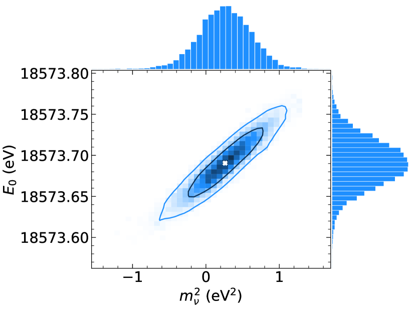
Figure 3: Distribution of fitted $m_{\nu}^{2}$ and $E_{0}$ values, obtained by the Monte-Carlo propagation technique (see section VII). The best fit is defined as the 1D weighted median of the distribution. The combined endpoint is calculated using the correlated mean of the 12 ring-wise endpoints per sample.

Table 2: Breakdown of uncertainties of the neutrino-mass-squared best fit, sorted by size. The uncertainties of the individual systematic effects are quoted in the main text.

Effect	$68.2\text{\,}\mathrm{\char 37\relax}$ CL uncertainty on $m_{\nu}^{2}$  ($\text{\,}{\mathrm{eV}}^{2}$)
Statistical	0.29
Non-Poissonian background	0.11
Source-potential variations	0.09
Scan-step-duration-dependent background	0.07
$qU$-dependent background	0.06
Magnetic fields	0.04
Molecular final-state distribution	0.02
Column density $\times$ inelastic scat. cross-section	0.01
Activity fluctuations	0.01
Energy-loss function	$<0.01$
Detector efficiency	$<0.01$
Theoretical corrections	$<0.01$
High voltage stability and reproducibility	$<0.01$
Total uncertainty	0.34

V Results and discussion

The $\chi^{2}$ minimisation reveals an excellent goodness of fit with a $\chi^{2}$ per degree of freedom of $0.9$, corresponding to a p-value of 0.8. For the best fit of the squared neutrino mass we find $\mbox{$m_{\nu}^{2}$}=0.26^{+0.34}_{-0.34}$\text{\,}{\mathrm{eV}}^{2}$$, see Fig. 3. The independent analysis methods agree within about $5\text{\,}\mathrm{\char 37\relax}$ percent of the total uncertainty. The total uncertainty on the fit is dominated by the statistical error followed by uncertainties of background parameters and the source electric potential. The full breakdown of uncertainties can be found in Tab. 2.

Based on the best-fit result we obtain an upper limit of $\mbox{$m_{\nu}$}<$0.9\text{\,}\mathrm{eV}$$ at $90\text{\,}\mathrm{\char 37\relax}$ CL, using the Lokhov-Tkachov method [50]. The Feldman-Cousins technique [51] yields the same limit for the obtained best fit. This result is slightly higher than the sensitivity of $0.7\text{\,}\mathrm{eV}$, due to the positive fit value, which is consistent with a $\approx 0.8\sigma$ statistical fluctuation assuming a true neutrino mass of zero. We also perform a Bayesian analysis of the data set, with a positive flat prior on $m_{\nu}^{2}$. The resulting Bayesian limit at $90\text{\,}\mathrm{\char 37\relax}$ credibility is $\mbox{$m_{\nu}$}<$0.85\text{\,}\mathrm{eV}$$.

The ring-averaged, fitted effective endpoint is $E_{0}=$18\,573.69\pm 0.03\text{\,}\mathrm{eV}$$. Taking into account the center-of-mass molecular recoil of $\ce{T2}$ ($1.72\text{\,}\mathrm{eV}$), as well as the absolute electric source potential $\phi_{\mathrm{WGTS}}$ ($\sigma(\phi_{\mathrm{WGTS}})=$0.6\text{\,}\mathrm{V}$$) and the work function of the main spectrometer $\phi_{\mathrm{MS}}$ ($\sigma(\phi_{\mathrm{MS}})=$0.06\text{\,}\mathrm{eV}$$), we find a $Q$-value of $18\,575.2\pm 0.6\text{\,}\mathrm{eV}$, which is consistent with the previous KATRIN neutrino-mass campaign ($18\,575.2\pm 0.5\text{\,}\mathrm{eV}$ [45]) and the calculated $Q$-value from the $\ce{{}^{3}He}-\ce{{}^{3}H}$ atomic mass difference of $18\,575.72\pm 0.07\text{\,}\mathrm{eV}$ [52]. The good agreement underlines the stability and accuracy of the absolute energy scale of the apparatus.

We combined the neutrino-mass results from this work with the previously published KATRIN (KNM1) result [45]. A simultaneous fit of both data sets yields $\mbox{$m_{\nu}^{2}$}=$0.1\pm 0.3\text{\,}{\mathrm{eV}}^{2}$$ and a corresponding upper limit of $\mbox{$m_{\nu}$}<$0.8\text{\,}\mathrm{eV}$$ at $90\text{\,}\mathrm{\char 37\relax}$ CL, based on Lokhov-Tkachov or the Feldman-Cousins technique. The same result is obtained when multiplying the $m_{\nu}^{2}$ distributions from Monte-Carlo propagation, or adding the $\chi^{2}$ profile of the individual fits. As both data sets are statistics-dominated, correlated systematic uncertainties between both campaigns are negligible. Furthermore, we investigated a Bayesian combination, where the KNM1 posterior distribution of $m_{\nu}^{2}$ is used as prior for the KNM2 analysis, yielding consistent results. More details on the combined analyses can be found in the supplementary material.

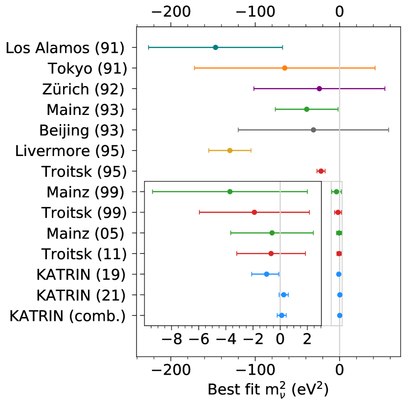
Figure 4: Comparison of best-fit values and uncertainties with previous neutrino mass experiments. References: Los Alamos 91 [53], Tokyo 91 [54], Zürich 92 [55], Mainz 93 [56], Beijing 93 [57], Livermore 95 [58], Troitsk 95 [59], Mainz 99 [60], Troitsk 99 [61], Mainz 05 [62], Troitsk 11 [63], KATRIN 19 [14, 15], KATRIN 21: this work, KATRIN combined: KATRIN 19 combined with KATRIN 21.

VI Conclusion and Outlook

The second neutrino-mass measurement campaign of KATRIN, presented here, is the first direct neutrino-mass measurement reaching sub-eV sensitivity ($0.7\text{\,}\mathrm{eV}$ at $90\text{\,}\mathrm{\char 37\relax}$ CL). Combined with the first campaign we set an improved upper limit of $\mbox{$m_{\nu}$}<$0.8\text{\,}\mathrm{eV}$$ ($90\text{\,}\mathrm{\char 37\relax}$ CL). We therefore have narrowed down the allowed range of quasi-degenerate neutrino-mass models and we have provided model-independent information about the neutrino mass, which allows the testing of non-standard cosmological models [64, 65]. Fig. 4 displays the evolution of best-fit $m_{\nu}^{2}$ results from historical neutrino-mass measurements up to the present day.

Compared to its previous measurement campaign, the KATRIN experiment has decreased the statistical and systematic uncertainties by about a factor of three and two, respectively. With the total planned measurement time of 1000 days, the total statistics of KATRIN will be increased by another factor of 50. A reduction of the background rate by a factor of two will be achieved by an optimised electromagnetic field design of the spectrometer section. Moreover, by eliminating the radon- and Penning-trap-induced background, the background-related systematic effects are expected to be significantly reduced. Together with a new high-rate krypton calibration scheme and a new method to improve the determination of the magnetic fields we will minimise the dominant systematic uncertainties to reach the target sensitivity of $m_{\nu}^{2}$ in the vicinity of $0.2\text{\,}\mathrm{eV}$.

High-precision $\upbeta$-spectroscopy with the KATRIN experiment has proven to be a powerful means to probe the neutrino mass with unprecedented sensitivity and to explore physics beyond the Standard Model, such as sterile neutrinos [66]. Together with cosmological probes and searches for neutrinoless double $\upbeta$-decay[67], the upcoming KATRIN data will play a key role in measuring the neutrino mass parameters.

VII Methods

In this section we describe the data analysis chain starting from the data processing to the high-level fit and limit setting. Moreover, we provide details on one of the key calibration campaigns, concerning the source electric potential. For a more extensive description of the KATRIN analysis procedure, the reader is referred to a recent publication [15].

VII.1 Data processing, selection, and combination

The first step of the analysis chain is the preparation of the data. Raw data are combined into integral spectral data points, which are then fitted with an analytical spectrum prediction including the response of the experiment.

Rate determination

The electrons which are transmitted through the main spectrometer are further accelerated by a post-acceleration electrode (PAE) with the potential $U_{\mathrm{PAE}}=$10\text{\,}\mathrm{keV}$$ before they are detected by the focal-plane detector [35]. The latter provides a high detection efficiency (>$95\text{\,}\mathrm{\char 37\relax}$) and a moderate energy resolution ($2.8\text{\,}\mathrm{keV}$ FWHM at $28\text{\,}\mathrm{keV}$). The total rate per pixel at a given retarding potential $qU_{i}$ is determined by integrating the rate in a wide and asymmetric region of interest (ROI) of $$14\text{\,}\mathrm{keV}$\leq E\leq$32\text{\,}\mathrm{keV}$$. The asymmetric ROI is chosen to account for energy losses in the deadlayer of the Si-PIN diodes [68], for partial energy deposition due to backscattering of electrons off the detector surface and due to charge sharing between pixels.

The detector efficiency slightly depends on $qU_{i}$. Three effects are considered: 1) The differential energy spectrum of the transmitted electrons at the FPD is shifted (and slightly scaled) according to $qU_{i}$. Since the same ROI is used for each $qU_{i}$, some electrons are no longer covered by the fixed ROI when lowering the potential, which effectively changes the detection efficiency. Based on reference measurements the relative reduction of detection efficiency at $E_{0}-$1\text{\,}\mathrm{keV}$$, with respect to the efficiency at $E_{0}$, is determined to be $\delta_{\mathrm{ROI}}=0.002$, with an uncertainty of $0.16\text{\,}\mathrm{\char 37\relax}$. The data is corrected according to the efficiency at the given $qU_{i}$ value. 2) As the counting rate at the focal plane detector depends on $qU_{i}$, so does the probability of pile-up. As the energy of most pile-up events is added, they are not covered by the ROI, thereby effectively changing the detector efficiency with $qU_{i}$. Based on a random-coincidence model assuming a Poisson-distributed signal, the relative reduction of efficiency at $E_{0}-$1\text{\,}\mathrm{keV}$$, with respect to the efficiency at $E_{0}$, is estimated to be $\delta_{\mathrm{PU}}=0.0002$, with an uncertainty of $18\text{\,}\mathrm{\char 37\relax}$. The data is corrected accordingly. 3) Finally, a significant fraction of about $20\text{\,}\mathrm{\char 37\relax}$ of all electrons impinging on the detector surface are backscattered. For low retarding potentials and small energy depositions in the detector, these backscattered electrons have a chance of remaining undetected by overcoming the retarding potential a second time in the direction towards the tritium source. The lower $qU_{i}$, the higher is the probability for lost electrons, effectively changing the detection efficiency. Based on Monte Carlo simulations, we estimate the efficiency reduction to be $\delta_{\mathrm{BS}}<0.001$ at $E_{0}-$1\text{\,}\mathrm{keV}$$. We neglect this effect in this analysis. Systematic uncertainties related to the efficiency corrections are negligibly small for the presented analysis, which only considers the last $40\text{\,}\mathrm{eV}$ of the tritium spectrum.

Selection of golden pixels and scans

The detector is segmented into 148 pixels of equal area. For the analysis 117 pixels have been chosen. The rejected pixels show undesirable characteristics such as broadened energy resolution, higher noise levels, or decreased rate due to misalignment of the beam-line with respect to the magnetic flux tube.

Out of the 397 scans recorded, 361 passed a strict quality assessment and were included in the neutrino mass analysis. The other runs were rejected for reasons of failed set-points of spectrometer electrodes and downtime of the Laser Raman system. The golden pixel and run selection is performed prior to the unblinding of the data.

Data combination

The 117 golden pixels are grouped into 12 detector rings and the detector counts recorded within each ring are summed to obtain 12 independent spectra. All golden scans are combined by adding the counts recorded at the same retarding energies. This method leads to a total number of data points of $n_{\mathrm{data}}=n_{qU}\times n_{\mathrm{rings}}=336$.

VII.2 Spectrum calculation

In order to infer the neutrino mass, the integral spectrum is fitted with the analytical spectrum calculation including the experimental response. As can be seen in Eq. (2), the theoretical spectrum is composed of the differential tritium spectrum $R_{\upbeta}(E)$ and the experimental response function $f(E,qU_{i})$. The differential spectrum is given by

$$\begin{split}R_{\mathrm{\upbeta}}(E)&=\frac{{G}_{\mathrm{F}}^{2}\cos^{2}{\Theta_{\mathrm{C}}}}{2\pi^{3}}|M_{\mathrm{nucl}}|^{2}F(E,Z^{\prime}=2)\\ &\cdot{(E+m_{e})}\sqrt{{(E+m_{e})}^{2}-m_{e}^{2}}\\ &\cdot\sum_{f}\zeta_{f}\,{\varepsilon_{f}(E)}\sqrt{{\varepsilon_{f}(E)}^{2}-m_{\nu}^{2}}\operatorname{\Theta}(\varepsilon_{f}(E)-m_{\nu}).\end{split}$$ (3)

with ${G}_{\mathrm{F}}$ denoting the Fermi constant, $\cos^{2}{\Theta_{\mathrm{C}}}$ the Cabibbo angle, $|M_{\mathrm{nucl}}|^{2}$ the energy-independent nuclear matrix element, and $F(E,Z^{\prime}=2)$ the Fermi function. While, $\varepsilon_{f}(E)={E_{0}}-V_{f}-E$, where ${E_{0}}$ denotes the maximum kinetic energy of the electron, in case of zero neutrino mass, and $V_{f}$ describe the molecular excitation energies, which are populated with the probabilities $\zeta_{f}$. $E$ and $m_{\mathrm{e}}$ denote the kinetic energy and mass of the $\upbeta$-electron, respectively.

Beyond the molecular effects, further theoretical corrections arise on the atomic and nuclear level [69]. Relevant for this analysis are only the radiative corrections to the differential spectrum, which are included in the analytical description, but not shown here. Furthermore, we emulate the effect of Doppler broadening as well as spatial and temporal source and spectrometer electric potential variations, by broadening the final state distribution with a Gaussian distribution.

The experimental response function

$$\begin{split}f(E-qU)&=\int_{\epsilon=0}^{E-qU}\!\int_{\theta=0}^{\theta_{\mathrm{max}}}\mathcal{T}(E-\epsilon,\theta,U)\sin\theta\\ &\cdot\sum_{s}P_{s}(\theta)\,f_{s}(\epsilon)\,d\theta\,d\epsilon~{}.\end{split}$$ (4)

depicts the probability of an electron with a starting energy $E$ to reach the detector. It combines the transmission function $\mathcal{T}(E-\epsilon,\theta,U)$ of the main spectrometer and the electron’s energy losses $\epsilon$ due to inelastic scattering with the tritium molecules in the source. The scattering energy losses are described by the product of the $s$-fold scattering probabilities $P_{s}(\theta)$, which depend on the path length through the source and hence on the pitch angle $\theta$, and the energy-loss function $f_{s}(\epsilon)$ for a given number of scatterings $s$. The energy-loss function is determined experimentally with the electron gun installed at the rear of the source. A typical response function and corresponding energy loss function is shown in Fig. 5.

The integrated transmission function for an isotropic source of electrons is given by

$$T (E,U)=\int_{\theta=0}^{\theta_{\text{max}}}\;\mathcal{T}(E,\theta,U)\cdot\sin\theta\,d\theta$$ (5)

$$=\left\{\begin{array}[]{ll}0&,\epsilon<0\\ 1-\sqrt{1-\frac{E-qU}{E}\frac{B_{\text{source}}}{B_{\mathrm{ana}}}\frac{2}{\gamma\!+\!1}}&,0\leq E-qU\leq\Delta E\\ 1-\sqrt{1-\frac{B_{\text{source}}}{B_{\text{max}}}}&,E-qU>\Delta E\end{array}\right.\,.$$ (9)

It is governed by the magnetic fields at the starting position $B_{\text{source}}$ of the electron, the maximum field $B_{\text{max}}$ in the beam line, and the magnetic field in the spectrometer’s analysing plane $B_{\mathrm{ana}}$. Synchrotron energy losses of $\upbeta$-electrons in the high magnetic field in the source and transport systems are included as an analytical correction to the transmission function (not shown here).

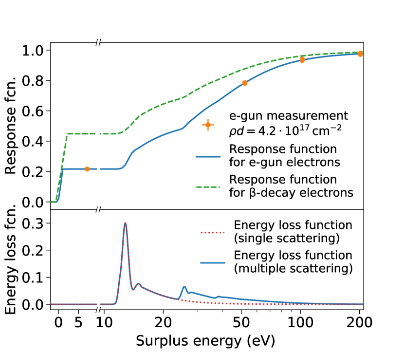
Figure 5: (Top) Electron-gun rate from multiple measurements at four surplus energies (yellow circles) and fitted response function of the electron-gun electrons (blue line) which start at the rear of the source for the best-fit column density of $\rho d=$4.2\text{\times}{10}^{17}\text{\,}{\mathrm{cm}}^{-2}$$ for that specific measurement. The green-dashed line illustrates the response function of the beta-decay electrons starting inside of the gaseous tritium source for the average column density during the neutrino mass measurement campaign of $\rho d=$4.2\text{\times}{10}^{17}\text{\,}{\mathrm{cm}}^{-2}$$. (Bottom) Energy-loss function for a single scattering process (red-dotted line) and multiple scatterings (blue line) as they occur for the measured $\rho d$ value.

Table 3: Overview of key figures for the second neutrino mass measurement campaign. When value and uncertainty are both given in %, then the statement is understood as $\left(\mathrm{value}\pm\mathrm{uncertainty}\right)\,\%$. ^∗The analysis interval refers to $qU_{i}\in\left(E_{0}-$40\text{\,}\mathrm{eV}$,E_{0}+$135\text{\,}\mathrm{eV}$\right)$.

	Value	Uncertainty
Average source parameters
Column density	$4.23\text{\times}{10}^{17}\text{\,}{\mathrm{cm}}^{-2}$	$0.25\text{\,}\mathrm{\char 37\relax}$
Source activity	$9.5\text{\times}{10}^{10}\text{\,}\mathrm{Bq}$	-
Relative activity variation within scan	$3.5\text{\times}{10}^{-4}\text{\,}$	-
Atomic tritium purity	0.987	0.003
Concentration T2	0.973	0.005
Concentration DT	0.0031	0.0004
Concentration HT	0.023	0.004
Source temperature	$30.065\text{\,}\mathrm{K}$	$0.001\text{\,}\mathrm{K}$
Final state distribution
Probability to decay to the ground state	$57\text{\,}\mathrm{\char 37\relax}$	$1\text{\,}\mathrm{\char 37\relax}$
Variance of ground state distribution	$0.2\text{\,}{\mathrm{eV}}^{2}$	$0.5\text{\,}\mathrm{\char 37\relax}$
Variance of FSD in analysis interval∗	$185.2\text{\,}{\mathrm{eV}}^{2}$	$1.2\text{\,}\mathrm{\char 37\relax}$
Source plasma parameters
Variance $\sigma_{\mathrm{P}}^{2}$	$12.4\text{\times}{10}^{-3}\text{\,}{\mathrm{eV}}^{2}$	$16.1\text{\times}{10}^{-3}\text{\,}{\mathrm{eV}}^{2}$
Rear-to-front asymmetry parameter $\Delta_{\mathrm{P}}$	$0\text{\,}\mathrm{meV}$	$61\text{\,}\mathrm{meV}$
Average magnetic fields
Source	$2.52\text{\,}\mathrm{T}$	$1.7\text{\,}\mathrm{\char 37\relax}$
Analysing plane	$6.308\text{\times}{10}^{-4}\text{\,}\mathrm{T}$	$1.0\text{\,}\mathrm{\char 37\relax}$
Maximum	$4.239\text{\,}\mathrm{T}$	$0.1\text{\,}\mathrm{\char 37\relax}$
Spectrometer parameters
Background	$220\text{\,}\mathrm{m}\mathrm{c}\mathrm{p}\mathrm{s}$	$0.8\text{\,}\mathrm{m}\mathrm{c}\mathrm{p}\mathrm{s}$
Background increase during scan step	$3\text{\,}\mathrm{\SIUnitSymbolMicro}\mathrm{c}\mathrm{p}\mathrm{s}\mathrm{/}\mathrm{s}$	$3\text{\,}\mathrm{\SIUnitSymbolMicro}\mathrm{c}\mathrm{p}\mathrm{s}\mathrm{/}\mathrm{s}$
Background qU linear dependence	$0\,\mathrm{mpcs/keV}$	$4.74\,\mathrm{mpcs/keV}$
Non-Poissonian background	$11.2\text{\,}\mathrm{\char 37\relax}$	-
High voltage stability and reproducibility	$13.5\text{\,}\mathrm{m}\mathrm{e}\mathrm{V}$	$0.8\text{\,}\mathrm{m}\mathrm{e}\mathrm{V}$
Detector parameters
Detector efficiency	$>$95\text{\,}\mathrm{\char 37\relax}$$	-
Region of Interest (ROI)	$14-$32\text{\,}\mathrm{keV}$$	-
Detector efficiency qU reduction (ROI)	$2\text{\times}{10}^{-3}\text{\,}$ ($1\text{\,}\mathrm{keV}$ below $E_{0}$)	$0.16\text{\,}\mathrm{\char 37\relax}$
Detector efficiency qU reduction (pile up)	$2\text{\times}{10}^{-4}\text{\,}$ ($1\text{\,}\mathrm{keV}$ below $E_{0}$)	$18\text{\,}\mathrm{\char 37\relax}$

VII.3 Systematic uncertainties

The analytical description $R(qU_{i},r_{j})$ of the integral $\upbeta$-spectrum, shown in Eq. (2), contains various signal- and background-related parameters, which are known with a certain accuracy. In the following we describe these parameters, their uncertainties, and their treatment in the neutrino mass analysis.

Signal-related systematic effects

The spectrum prediction includes uncertainties of the nine parameters of the empirical energy loss function (the individual relative uncertainties of the parameters $\sigma_{\mathrm{eloss},k}$ are between $0.016\text{\,}\mathrm{\char 37\relax}$ and $3.8\text{\,}\mathrm{\char 37\relax}$), a relative uncertainty of the product of column density and scattering cross-section ($\sigma_{\rho d\times\sigma}=$0.25\text{\,}\mathrm{\char 37\relax}$$), relative uncertainties of the theoretical description of the molecular final-state distribution ($\sigma_{\mathrm{FSD}}=\mathcal{O}($1\text{\,}\mathrm{\char 37\relax}$)$), and relative uncertainties of the magnetic field in the source ($\sigma_{B_{\mathrm{source}}}=$1.7\text{\,}\mathrm{\char 37\relax}$$), in the analysing plane ($\sigma_{B_{\mathrm{ana}}}=$1\text{\,}\mathrm{\char 37\relax}$$), and the maximal field ($\sigma_{B_{\mathrm{max}}}=$0.1\text{\,}\mathrm{\char 37\relax}$$). The variations of the $\upbeta$-decay activity during a scan ($\sigma_{\mathrm{scan}}=$0.03\text{\,}\mathrm{\char 37\relax}$$) were negligibly small.

The spatial and temporal variations of the source electric potential were not included in the first neutrino mass campaign. With the increase of the source column density from $1.11\text{\times}{10}^{17}\text{\,}{\mathrm{cm}}^{-2}$ to $4.23\text{\times}{10}^{17}\text{\,}{\mathrm{cm}}^{-2}$ in this campaign, the creation rates and densities of the charge carriers, as well as the fraction of scattered electrons, increased accordingly, which makes plasma effects more relevant [12, 70, 71]. A detailed description of the plasma calibration is given in Sec. VII.4.

Background-related systematic effects

Electrons created in a radon decay in the main spectrometer volume can initially be magnetically trapped. These trapped electrons can create a cluster of 10 - 100 secondary electrons [20] by scattering off the residual gas in the main spectrometer, which is operated at a pressure of $10^{-11}$ mbar. These secondary electrons arrive at the detector within a time window of about $1000\text{\,}\mathrm{s}$, hence leading to a non-Poissonian rate distribution. The observed background rate can be modelled by a Gaussian distribution, with a width $11.2\text{\,}\mathrm{\char 37\relax}$ wider than expected from a purely Poisson distribution. This overdispersion is treated as an increased statistical uncertainty in the analysis.

As the transmission conditions for the background electrons slightly depend on the retarding-potential setting, a small retarding-potential dependence of the background can occur. In the analysis, we allow for a linear dependence of the background on the retarding potential and use dedicated test measurements to constrain the possible slope to $m^{qU}_{\mathrm{bg}}=$0\pm 4.74\text{\,}\mathrm{m}\mathrm{c}\mathrm{p}\mathrm{s}\mathrm{/}\mathrm{k}\mathrm{eV}$$.

Finally, the pre- and main spectrometers, being both operated at high voltage, create a Penning trap between them. Stored electrons and the subsequently produced positive ions, which can escape the trap into the main spectrometer, are a source of background, as illustrated in Fig. 1. To mitigate this background, the trap is emptied with an electron-catcher system [72] after each scan step. However, a potentially small increase of the background rate within a scan step cannot be excluded, which could lead to a background dependence on the duration of the scan step. By fitting a linear increase to the rate evolution within all scan steps we find a slope of $m^{\mathrm{t}_{\mathrm{scan}}}_{\mathrm{bg}}=$3\pm 3\text{\,}\mathrm{\SIUnitSymbolMicro}\mathrm{c}\mathrm{p}\mathrm{s}\mathrm{/}\mathrm{s}$$, which is included in the $\upbeta$-spectrum fit .

VII.4 Source Potential Calibration

The absolute electric potential of the source does not affect the spectral shape of the measured spectrum. An unknown absolute source potential is largely absorbed by the effective endpoint, which is a free parameter in the fit. A change of the effective endpoint mostly leads to a shift of the spectrum and has a negligible effect on the spectral shape. Accordingly, an unknown radial variation of the electric potential is in good approximation absorbed by the ring-wise endpoint parameters. Consequently, these effect have a minor impact on the neutrino mass analysis. However, any temporal or longitudinal variations of the source potential can lead to spectral distortions, which are parameterised by a Gaussian broadening $\sigma_{\mathrm{P}}$ and the parameter $\Delta_{\mathrm{P}}$ which quantifies the longitudinal rear-to-front asymmetry of the electric potential of the source. This asymmetry of the potential results in a shift of the energy spectrum associated with scattered electrons (predominantly originating from the rear of the source tube) compared to the spectrum of the unscattered electrons (predominantly originating from the front of the source tube).

Both parameters are assessed with the help of co-circulating ${}^{83\mathrm{m}}\mathrm{Kr}$ gas. The spectroscopy of its mono-energetic conversion electron lines reveals information about the broadening $\sigma_{\mathrm{P}}$ of the line shape, from which an upper limit of $\Delta_{\mathrm{P}}$ is derived.

The calibration was performed at an elevated source temperature of $T=$80\text{\,}\mathrm{K}$$ to prevent condensation of the Kr gas (as compared to the $T=$30\text{\,}\mathrm{K}$$ set-point used during neutrino-mass measurements). The tritium circulation loop of the tritium source [73] can be operated in two modes, a) in a mode with direct-recycling of the krypton-tritium mixture which is limited to a maximum column density of $40\text{\,}\mathrm{\char 37\relax}$ ($2.08\text{\times}{10}^{17}\text{\,}{\mathrm{cm}}^{-2}$), but delivers a high krypton rate, and b) in a mode of fractional direct-recycling which can be operated up to $75\text{\,}\mathrm{\char 37\relax}$ ($3.75\text{\times}{10}^{17}\text{\,}{\mathrm{cm}}^{-2}$) of the nominal column density, but with only about $0.5\text{\,}\mathrm{\char 37\relax}$ of the maximum krypton activity as compared to mode a).

The plasma parameters are inferred by combining the measurements of the internal conversion lines N_2,3-32 and L₃-32. The energy of the conversion electrons, emitted from a particular subshell of the ${}^{83\mathrm{m}}\mathrm{Kr}$ atom, is $30\,472.6\text{\,}\mathrm{eV}$ for the L₃-32 singlet and $32\,137.1\text{\,}\mathrm{eV}$ ($32\,137.8\text{\,}\mathrm{eV}$) for the N_2,3-32 doublet [74]. The L₃-32-line, on the one hand, has a high intensity, but its natural line width is not known precisely [75]. The N_2,3-32-lines, on the other hand, have a low intensity, but their natural line width is negligible compared to a spectral broadening caused by variations of the electric potential. Thus, any broadening of the N_2,3-32-lines beyond the known spectrometer resolution and the thermal Doppler broadening can be assigned to variations of the electric potential within the source. Based on the N_2,3-32-line doublet measurement at $40\text{\,}\mathrm{\char 37\relax}$ of the nominal column density we find $\sigma_{\mathrm{P}}^{2}($40\text{\,}\mathrm{\char 37\relax}$)=\left(1.4\pm 0.3\right)10^{-3}$\text{\,}{\mathrm{eV}}^{2}$$ (See Fig. 6). Combined with L₃-32-line measurements both at $40\text{\,}\mathrm{\char 37\relax}$ and $75\text{\,}\mathrm{\char 37\relax}$ of the nominal column density, we assess the relative change of the broadening and find $\sigma_{\mathrm{P}}^{2}($75\text{\,}\mathrm{\char 37\relax}$)=\left(8.0\pm 8.2\right)10^{-3}$\text{\,}{\mathrm{eV}}^{2}$$. Finally, we conservatively extrapolate with exponential scaling this value to $84\text{\,}\mathrm{\char 37\relax}$ of the nominal column density, leading to $\sigma_{\mathrm{P}}^{2}($84\text{\,}\mathrm{\char 37\relax}$)=\left(12.4\pm 16.1\right)10^{-3}$\text{\,}{\mathrm{eV}}^{2}$$.

In the analysis, we limit the broadening $\sigma_{\mathrm{P}}$ to positive values. We construct the probability density function of the asymmetry parameter $\Delta_{\mathrm{P}}$ based on phenomenological considerations on the relation of both plasma parameters given by $|\Delta_{\text{P}}|\leq\sigma_{\mathrm{P}}/{1.3}$  [76]. For many samples of $\sigma_{\mathrm{P}}^{2}$ we draw a value for $\Delta_{\mathrm{P}}$ from a uniform distribution in the range $-\sigma_{\mathrm{P}}/1.3\leq\Delta_{\mathrm{P}}\leq\sigma_{\mathrm{P}}/1.3$. The resulting distribution can be approximated by a Gaussian distribution centred around $0\text{\,}\mathrm{meV}$ with a width of $61\text{\,}\mathrm{meV}$.

We expect to reduce the systematic uncertainties in future campaigns by operating the tritium source at the same temperature during the neutrino-mass and krypton measurements, and by using an ultra-high intensity krypton source (with about $10\text{\,}\mathrm{GBq}$ of the ⁸³Rb mother isotope), which will make the N_2,3-32-line measurement possible at nominal column density (mode b).

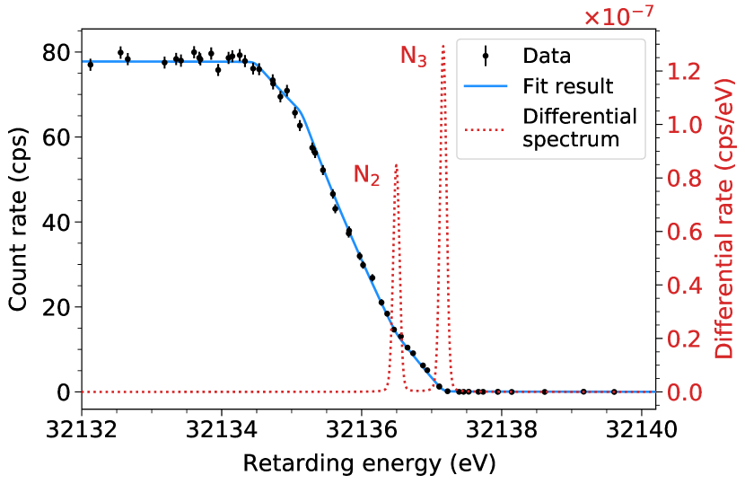
Figure 6: $N_{2}$/$N_{3}$ doublet (internal conversion lines of ^83mKr) at $40\text{\,}\mathrm{\char 37\relax}$ of the nominal column density for a sample data spectrum. The visible width of the integrated spectrum is dominated be the energy resolution. The differential line width represents the broadening by fitted $\sigma_{\mathrm{P}}^{2}$ only. The Doppler line width from the thermal movement of the Kr atoms is not displayed. The goodness-of-fit is $\chi^{2}/\mathrm{ndof}=68.2/52=1.3$ and the p-value is $6.6\times 10^{-2}$.

VII.5 Parameter inference

We infer the parameters of interest via a minimisation of the $\chi^{2}$ function

$$\begin{split}\chi^{2}=&\left(\vec{R}_{\mathrm{data}}(q\vec{U},\vec{r})-\vec{R}(q\vec{U},\vec{r}|\vec{\Theta},\vec{\eta})\right)^{T}\\ &\cdot C^{-1}\left(\vec{R}_{\mathrm{data}}(q\vec{U},\vec{r})-\vec{R}(q\vec{U},\vec{r}|\vec{\Theta},\vec{\eta})\right),\end{split}$$ (10)

where $\vec{R}_{\mathrm{data}}(q\vec{U},\vec{r})$ gives the measured count rates at a retarding potential $qU_{i}$ for the detector ring $r_{j}$, $\vec{R}(q\vec{U},\vec{r})$ gives the predictions of these rate, and $C$ is the covariance matrix that includes the statistical uncertainties and can be used to also describe systematic uncertainties. The usage of a $\chi^{2}$ minimisation is justified, as the numbers of electrons per scan-step $qU_{i}$ and detector ring $r_{j}$ are sufficiently large (> 700) to be described by a Gaussian distribution, instead of a Poisson distribution.

The fit has $1+3\times 12=37$ free parameters $\vec{\Theta}$, including a single parameter for the neutrino mass squared $m_{\nu}^{2}$, and 12 ring-wise values for each of the three spectral parameters: the normalisation factor $A_{\mathrm{s}}$, the background rate $R_{\mathrm{bg}}$, and the effective endpoint $E_{0}$. In addition, the spectrum depends on systematic parameters $\vec{\eta}$ (as found in Tab.  3), such as the column density, tritium isotopologue concentrations, magnetic fields, etc. These parameters are known with a certain accuracy and their uncertainty needs to be propagated to the final neutrino mass result. Four different methods are used for the KATRIN analysis:

Pull method

In the ‘pull method’ the systematic parameters $\eta_{i}$ are treated as free parameters in the fit and introduced as nuisance terms in the $\chi^{2}$ function

$$\chi^{2}(\vec{\Theta},\vec{\eta}) =\chi^{2}(\vec{\Theta},\vec{\eta})+\sum_{i}\left(\frac{\hat{\eta_{i}}-\eta_{i}}{\sigma_{\eta_{i}}}\right)^{2}~{}.$$ (11)

The nuisance terms allow the parameter to vary around its best estimation $\hat{\eta_{i}}$ according to its uncertainty $\sigma_{\eta_{i}}$ as determined from external measurements

This method is computationally intensive due to the complexity in calculating the tritium spectrum and the minimisation with respect to multiple free parameters. For example, it is not practical to treat the uncertainties of the molecular final state distribution, which is given as a discrete list of excitation energies and corresponding probabilities, with this method. The advantage of this method is that we make the maximum use of the data. If the spectral data contain information about the systematic parameters $\vec{\eta}$, it is automatically taken into account.

Covariance matrix method

As can be seen in Eq. (VII.5), the standard $\chi^{2}$ estimator includes a covariance matrix $C$ which can describe both the statistical and systematic model uncertainties. The diagonal entries describe the uncertainties which are uncorrelated for each $R(qU_{i},r_{j})$, while the off-diagonal terms describe the correlated uncertainties between the $R(qU_{i},r_{j})$. The covariance matrix $C$ is computed by simulating $\mathcal{O}(10^{4})$ $\upbeta$-spectra, with the systematic parameters $\eta_{i}$ varied according to their probability density functions in each spectrum. From the resulting set of spectra, the variance and covariance of the spectral points $R(qU_{i},r_{j})$ are determined.

As the covariance matrices for individual or combined systematic effects are computed before fitting, this method is efficient with respect to computational costs. The dimension of the covariance matrix is given by the number of data points. Therefore, the efforts for matrix calculation and inversion can be diminished by reducing the number of data points.

Monte-Carlo propagation method

Generally, in the Monte-Carlo (MC) propagation technique, the uncertainties of the parameters $\eta_{i}$ are propagated by repeating the fit about $10^{5}$ times, with the systematic parameters varied according to their probability density functions each time. The method then returns the distributions of the fit parameters $\vec{\Theta}$, which reflect the uncertainty of the systematic parameters.

More precisely, when assessing the systematic effects alone, a MC spectrum without statistical fluctuations is created (based on the best fit parameters), which is then fitted $10^{5}$ times with a model, which systematic parameters of interest are varied each time. Contrarily, when evaluating the statistical uncertainty alone, $10^{5}$ statistically randomized MC spectra are created and fitted with a constant model. Accordingly, for obtaining the total uncertainty, both steps are combined.

To extract information on the parameters $\vec{\eta}$ from the data itself, each entry in the resulting histogram of best fit parameters is weighted with the likelihood of the corresponding fit. The final distributions are then used to estimate the best-fit values (mode of the distribution) and uncertainty (integration of the distribution up to $16\text{\,}\mathrm{\char 37\relax}$ from both side).

The advantage of this method is that the number of free parameters is kept at a minimum, which facilitates the minimisation procedure. The larger number of fits, however, is time consuming and requires the usage of large computing clusters.

Bayesian Inference

In Bayesian inference one computes the posterior probability for the parameters of interest $\vec{\Theta}$ from a prior probability and a likelihood function according to Bayes’ theorem. For the KATRIN analysis, the Bayesian approach has the advantage that prior knowledge on the neutrino mass can naturally be applied via a corresponding informative prior. For example, the prior of $m_{\nu}^{2}$ can be chosen to be flat and positive, which restricts the posterior distribution to the physically allowed regime and changes the credibility interval accordingly.

Ideally, all systematic effects $\eta_{i}$ would be included as free parameters constrained with our prior knowledge on the parameter. However, due to the computationally expensive spectrum calculation and the fact that the Bayesian inference requires a large number of samples in the Markov chain for sampling the posterior distribution, only the $qU$-dependent background is currently treated in this way. All other systematic uncertainties are included with a covariance matrix in the likelihood or by model variation (MV). For the MV, a large set of Markov Chains is started with randomized but fixed model variations. The randomisations are drawn from the systematic uncertainty distributions. The resulting set of posterior distributions is averaged.

VII.6 Limit Setting

We present two frequentist methods and one Bayesian method for the construction of an upper limit of the neutrino mass. For the former we use the classical Feldman-Cousins [51] and the Lokhov-Tkachov [50] belt constructions depicted in Fig. 7. In the Feldman-Cousins technique the acceptance region for $\widehat{m}_{\nu}^{2}$ is determined by ordering this estimator according to the likelihood ratio $\frac{\mathcal{L}\left(\widehat{m}_{\nu}^{2}\,|\,m_{\nu}^{2}\right)}{\mathcal{L}\left(\widehat{m}_{\nu}^{2}\,|\,\mathrm{max}(0,\,\widehat{m}_{\nu}^{2})\right)}$ for a given best-fit neutrino mass squared $m_{\nu}^{2}$. This method leads to more stringent upper limits for increasingly negative best-fit values. The method of Lokhov-Tkachov avoids this feature by using the standard Neyman belt-construction for positive values of $\widehat{m}_{\nu}^{2}$ and defining the experimental sensitivity as the upper limit in the non-physical regime of $\widehat{m}_{\nu}^{2}<0$.

The Bayesian $90\text{\,}\mathrm{\char 37\relax}$ credibility interval is obtained by integrating the posterior distribution of $m_{\nu}^{2}$ from zero to $\mbox{$m_{\nu}^{2}$}^{\mathrm{limit}}$, such that the total probability is $90\text{\,}\mathrm{\char 37\relax}$ as demonstrated in Fig. 8. Note that the interpretation of the limit obtained in this way is different from the frequentist confidence limits and hence the numerical values may not coincide.

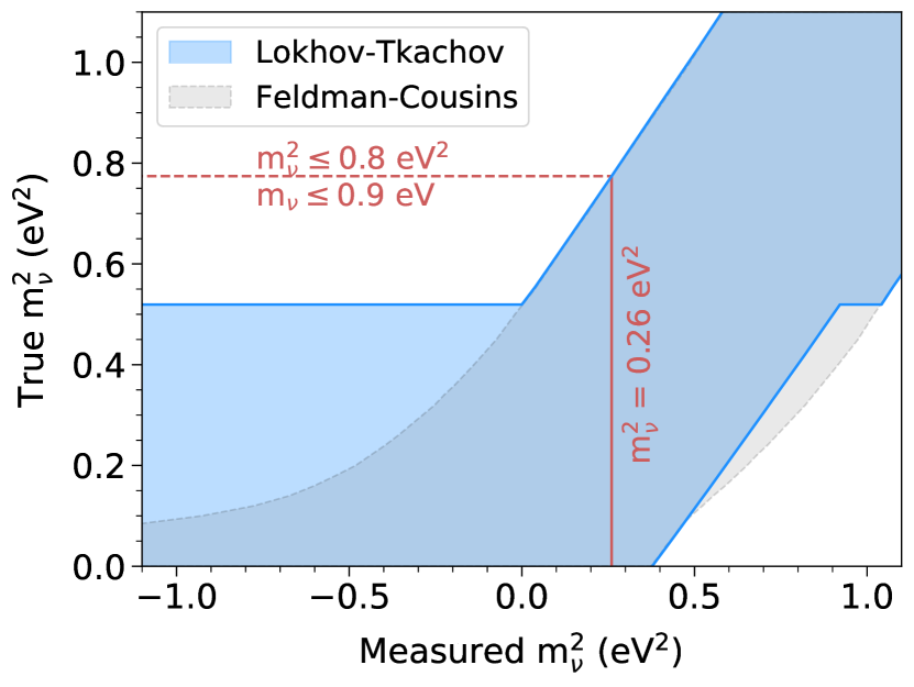
Figure 7: Frequentist bounds on the neutrino mass for the KNM2 dataset by using the constructions by Lokhov-Tkachov[50] and Feldman-Cousins [51].

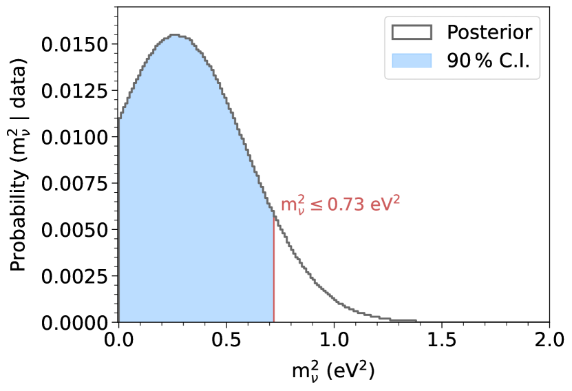
Figure 8: Posterior distribution of $m_{\nu}^{2}$ in the Bayesian analysis with a flat positive prior.

VII.7 Results of individual strategies

The frequentist analyses are performed by three independent teams, which use differing implementations of the spectral calculation and different strategies to propagate systematic uncertainties. A Bayesian analysis is performed, which interfaces to one of the spectrum calculation softwares. The analysis by independent teams is a powerful means to cross-check individual analyses. The following four data analysis strategies were applied to the second data set of KATRIN.

• Strategy 1 is based on a C++ framework [77] using the Minuit minimiser. It employs mainly the pull method for handling of systematics. We note that for the presented analysis, the input value for the ‘scan-step-duration-dependent background’ was corrected after the official unblinding of the data.

• Strategy 2 is implemented in a MATLAB framework and exclusively uses the covariance matrix approach to propagate systematic uncertainties [78]. We note that for the presented analysis, the ‘scan-step-duration-dependent background’ systematic was implemented only after the official unblinding of the data.

• Strategy 3 is based on a C++ framework using a custom-developed minimiser [79, 80]. In this strategy mostly the MC-propagation of uncertainties is applied.

• Strategy 4 performs a Bayesian interpretation of the data. For this approach the spectrum calculation software of ‘strategy 3’ is interfaced with the Bayesian Analysis Toolkit (BAT) [81]. Here, most of the systematic uncertainties are treated via the model variation (MV) technique.

An overview of the strategies is found in Tab.  4. The resulting best fit and systematic uncertainty breakdown are listed in Tab. 5.

Table 4: Overview of the analysis strategies. Abbreviations: pseudo-ring: combination of three detector rings; PT = Pull term method; MC = Monte-Carlo propagation method; CM = Covariance matrix method; MV = Model variation method; param. prior = using a Bayesian prior according to parameter uncertainties. The non-Poissionan background is included as an additional statistical (stat) error.

Item	Strategy
	1 (Pull term)	2 (Cov. matrix)	3 (MC prop.)	4 (Bayesian)
Minimisation	$\chi^{2}$	$\chi^{2}$	$\chi^{2}$	posterior
Detector pixel combination	12 rings	4 pseudo-rings	12 rings	4 pseudo-rings
Scan combination	stacking	stacking	stacking	stacking
Non-Poissonian background	stat	stat	stat	stat
Source potential variations	PT	CM	MC	MV
Scan step-duration-dependent background	PT	CM	MC	MV
$qU$-dependent background	PT	CM	MC	param. prior
Magnetic fields	PT	CM	MC	MV
Molecular final-state distribution	CM	CM	MC	CM
Column density $\times$ cross-section	PT	CM	MC	MV
Scan step fluctuations	CM	CM	CM	CM
Energy loss	PT	CM	MC	MV
Detector efficiency	-	CM	-	-
Theoretical corrections	-	CM	-	-
High voltage fluctuations	-	CM	-	-

Table 5: Breakdown of uncertainties of the neutrino mass best fit for each analysis. Strategy 1, 2, and 4 obtain the systematic uncertainty by quadratically subtracting the statistical error from the total uncertainty, while strategy 3 assesses the systematic uncertainty directly. Strategy 4 estimates the impact of individual systematic uncertainties in fits in which all detector pixels are combined, while the other strategies use a (pseudo-)ring-dependent fit (as explained in the main text). Differences in the second digit mainly arise from numerical effects.

	Strategies
	1 (Pull term)	2 (Cov. matrix)	3 (MC prop.)	4 (Bayesian)
$m_{\nu}^{2}$ best fit ($\text{\,}{\mathrm{eV}}^{2}$)	0.25	0.26	0.26	0.26
	$68.2\text{\,}\mathrm{\char 37\relax}$ CL uncertainties ($\text{\,}{\mathrm{eV}}^{2}$)
Statistical	0.28	0.28	0.29	0.31
Systematic	0.20	0.16	0.18	0.14
Total uncertainty	0.35	0.32	0.34	0.34
$\chi^{2}$ per degree of freedom	280.2/299 = 0.94	87.9/99 = 0.89	277.3/299 = 0.93	-
	breakdown of systematic uncertainties ($\text{\,}{\mathrm{eV}}^{2}$)
Non-Poissonian background	0.10	0.10	0.11	0.11
Source potential variations	0.09	0.07	0.07	0.07
Scan step-duration-dependent background	0.07	0.07	0.07	0.04
$qU$-dependent background	0.06	0.05	0.04	0.06
Magnetic fields	0.04	0.03	0.03	0.03
Molecular final-state distribution	0.02	0.01	0.01	0.01
Column density $\times$ inelastic scat. cross-section	0.01	0.01	0.01	0.01
Scan step fluctuations	< 0.01	< 0.01	0.01	< 0.03
Energy loss	< 0.01	< 0.01	< 0.01	0.02
Detector efficiency	neglected	< 0.01	neglected	neglected
Theoretical corrections	neglected	< 0.01	neglected	neglected
High voltage fluctuations	neglected	< 0.01	neglected	neglected

Supplementary information

VIII Combined analysis of first and second neutrino mass campaign

The 1000 days of total measurement time of the KATRIN experiment will be distributed within 15-20 individual measurement campaigns. The experimental parameters will not be constant over all these campaigns, as the systematic uncertainties are reduced and the experimental performance is improved (e.g. the background rate will be lowered) with time. Nevertheless, all individual campaigns need to be combined eventually to achieve the full statistical power.

VIII.1 Combination of individual results

One approach is to simply multiply the $m_{\nu}^{2}$ distributions obtained with MC-propagation of the individual measurement phases. As the uncertainties of the first and second neutrino mass campaigns are still largely statistically dominated and the main systematic uncertainties are uncorrelated, this method is well justified for the combination presented here. The best fit, obtained from the combined distribution is $\mbox{$m_{\nu}^{2}$}=$0.11\pm 0.34\text{\,}{\mathrm{eV}}^{2}$$. Assuming a symmetric Gaussian distribution of $m_{\nu}^{2}$, we derive an upper limit of $\mbox{$m_{\nu}$}<$0.81\text{\,}\mathrm{eV}$$ ( $90\text{\,}\mathrm{\char 37\relax}$ C.L). Adding the $\chi^{2}$-profiles of the individual fits leads to statistically consistent results.

VIII.2 Simultaneous fit of the both neutrino mass campaigns

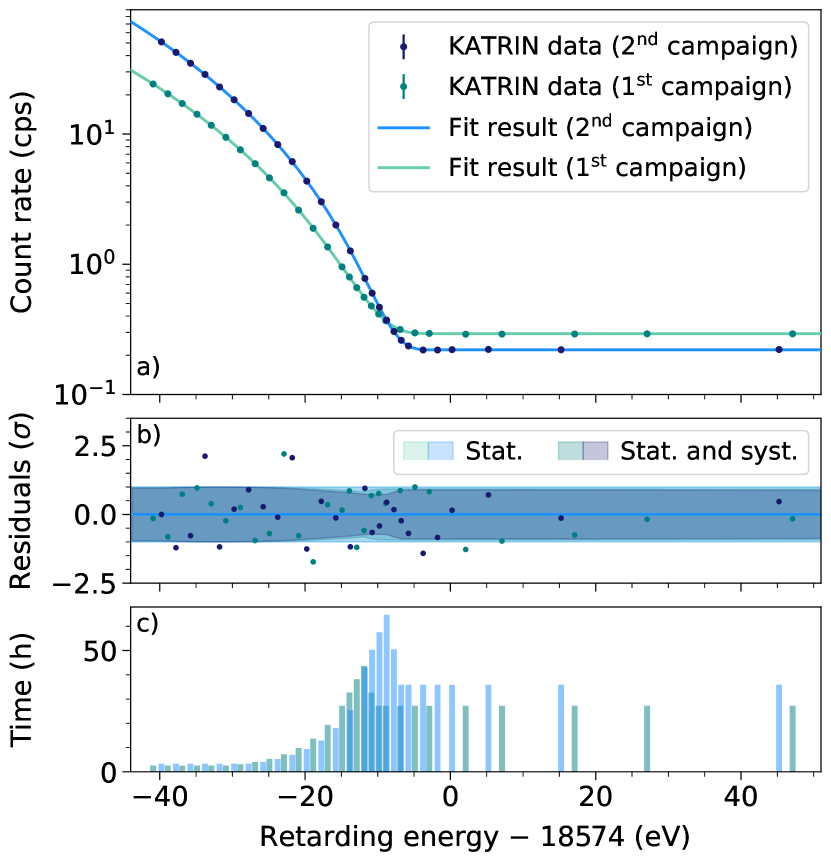
Figure 9: Simultaneous fit to the data of both the neutrino mass campaigns (KNM1 in green and KNM2 in blue) where the measured rates of the 12 detector rings are combined to a single detector area (uniform fit) in both campaigns. The combined best fit result is $\mbox{$m_{\nu}^{2}$}=$0.08\pm 0.32\text{\,}{\mathrm{eV}}^{2}$$. b) Normalised residuals for the fit to the data. c) Measurement time distribution for KNM1 and KNM2. Both have 28 scan steps with slightly differing retarding energies. The most sensitive region of the spectrum where most of the measurement time is spent is shifted slightly to higher energies in the KNM2 campaign due to the improved signal to background.

Another way, to combine both data sets, is by performing a simultaneous fit of both data sets with a common neutrino mass. The first and second neutrino mass campaigns were performed under different experimental conditions, e.g. the column density was increased by a factor of four and the background level was reduced by $25\text{\,}\mathrm{\char 37\relax}$ in the second campaign. Correspondingly, the systematic parameters and their uncertainties are partly different in the two campaigns. As a consequence, the data of the two campaigns cannot be described with a single effective spectrum prediction. Nevertheless, a simultaneous fit of both data sets can be performed by extending the $\chi^{2}$ function to

$$\begin{split}\chi^{2}&(\mbox{$m_{\nu}^{2}$},\vec{\Theta}_{p1},\vec{\Theta}_{p2},\vec{\eta}_{p1},\vec{\eta}_{p2},\vec{\eta}_{c})=\\ &\chi^{2}(\mbox{$m_{\nu}^{2}$},\vec{\Theta}_{p1},\vec{\eta}_{p1},\vec{\eta}_{c})+\chi^{2}(\mbox{$m_{\nu}^{2}$},\vec{\Theta}_{p2},\vec{\eta}_{p2},\vec{\eta}_{c})+\mathrm{pull\,terms}\end{split}$$ (12)

where $\vec{\Theta}_{p1}$ and $\vec{\Theta}_{p2}$ depict the endpoint, background, and normalisation of the first ($p1$) and second ($p2$) measurement period. These parameters can be different in the two measurement phases, as the experimental conditions are changed. $\vec{\eta}_{p1}$ and $\vec{\eta}_{p2}$ correspond to the two sets of systematic parameters, while $\vec{\eta}_{c}$ illustrates the set of common systematic parameters. The neutrino mass squared $m_{\nu}^{2}$  is a common parameter of both $\chi^{2}$ functions.

For a simultaneous fit the number of free parameters and data points increases by about a factor of two compared to the fit of a single measurement campaign, which makes the minimisation computationally challenging and prone to numerical noise. To simplify the problem, we choose for this analysis to group the detector rings to one effective detector area (uniform fit), reducing the number of free parameters to $n_{\mathrm{free}}=33$ and the number of data points to $n_{\mathrm{data}}=56$.

With respect to the stand-alone first neutrino mass analysis as presented in [15], the spectrum calculation has been slightly improved. It now includes the transmission function for non-isotropic electrons, an improved parametrisation of the energy loss function, and a reduced uncertainty on the magnetic fields and column density. Finally, a possible Penning-trap induced time-dependent background, as described in the main text, is included. A re-analysis of the first neutrino mass data with these new inputs reveals a best fit of $\mbox{$m_{\nu}^{2}$}=-1.0^{+0.9}_{-1.0}\,\mathrm{eV^{2}}$ and an upper limit of $\mbox{$m_{\nu}$}<$1.1\text{\,}\mathrm{eV}$$ at $90\text{\,}\mathrm{\char 37\relax}$ C.L. These values are in good ($10\text{\,}\mathrm{\char 37\relax}$) agreement with respect to the published result in [14].

The fit to both data sets is shown in Fig. 9. The $\chi^{2}/\mathrm{ndof}=51.7/49=1.1$ indicates excellent agreement of the model to the data. The final result of the combined fit reveals $\mbox{$m_{\nu}^{2}$}=$0.08\pm 0.32\text{\,}{\mathrm{eV}}^{2}$$ and a corresponding upper limit of $\mbox{$m_{\nu}$}<$0.76\text{\,}\mathrm{eV}$$ ($90\text{\,}\mathrm{\char 37\relax}$ CL).

In complement to the standard goodness-of-fit, we perform the Parameter-Goodness-of-Fit (PGoF) test [82] to assess the compatibility of KNM1 and KNM2 data sets. This test quantifies the penalty of combining the data sets compared to fitting them independently. We find a PGoF probability of $17\text{\,}\mathrm{\char 37\relax}$ reflecting a good agreement between the two statistically independent data sets.

VIII.3 Bayesian combination of both neutrino mass campaigns

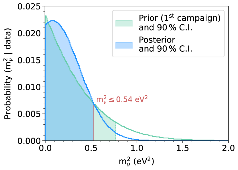
Figure 10: Posterior distributions of the observable $m_{\nu}^{2}$. The prior distribution for the KNM2 analysis (green) [15] is the posterior distribution from the KNM1 analysis. The resulting posterior distribution for the second campaign is shown in blue.

Another way of combining different neutrino mass measurement campaigns is by using the posterior distribution of one campaign as prior information for the other campaign. In this procedure, correlations between the data sets are neglected.

For the analysis of the first neutrino mass measurement campaign, we use the result published in [72], which includes the five major systematic effects. The resulting posterior distribution for $m_{\nu}^{2}$, displayed in Fig.  8, is then used as prior distribution of $m_{\nu}^{2}$ for the analysis of the second neutrino mass measurement campaign, which is otherwise performed with the same procedure as the stand-alone analysis.

The central value is found to be $\mbox{$m_{\nu}^{2}$}=$0.06\pm 0.32\text{\,}{\mathrm{eV}}^{2}$$. The corresponding $90\text{\,}\mathrm{\char 37\relax}$ credible interval from a positive prior on $m_{\nu}^{2}$ corresponds to a Bayesian limit of $\mbox{$m_{\nu}$}<$0.72\text{\,}\mathrm{eV}$$, as illustrated in Fig. 10.

References

- [1] Fukuda, Y. et al. Evidence for oscillation of atmospheric neutrinos. Phys. Rev. Lett. 81, 1562–1567, DOI: 10.1103/PhysRevLett.81.1562 (1998). eprint hep-ex/9807003.
- [2] Ahmad, Q. R. et al. Direct evidence for neutrino flavor transformation from neutral-current interactions in the Sudbury Neutrino Observatory. Phys. Rev. Lett. 89, 011301, DOI: 10.1103/PhysRevLett.89.011301 (2002). eprint nucl-ex/0204008.
- [3] Petcov, S. T. The Nature of Massive Neutrinos. Adv. High Energy Phys. 2013, 852987, DOI: 10.1155/2013/852987 (2013).
- [4] Agarwal, S. & Feldman, H. A. The effect of massive neutrinos on the matter power spectrum. Monthly Notices of the Royal Astronomical Society 410, 1647–1654, DOI: 10.1111/j.1365-2966.2010.17546.x (2011).
- [5] Lesgourgues, J. & Pastor, S. Massive neutrinos and cosmology. Physics Reports 429, 307 – 379, DOI: https://doi.org/10.1016/j.physrep.2006.04.001 (2006).
- [6] Alam, S. et al. Completed SDSS-IV extended Baryon Oscillation Spectroscopic Survey: Cosmological implications from two decades of spectroscopic surveys at the Apache Point Observatory. Phys. Rev. D 103, 083533, DOI: 10.1103/PhysRevD.103.083533 (2021). eprint 2007.08991.
- [7] Aghanim, N. et al. Planck 2018 results. VI. Cosmological parameters. Astron. Astrophys. DOI: 10.1051/0004-6361/201833910 (2020). eprint 1807.06209.
- [8] Di Valentino, E., Melchiorri, A. & Silk, J. Beyond six parameters: Extending cdm. Phys. Rev. D 92, 121302, DOI: 10.1103/PhysRevD.92.121302 (2015).
- [9] Boyle, A. & Komatsu, E. Deconstructing the neutrino mass constraint from galaxy redshift surveys. JCAP 03, 035, DOI: 10.1088/1475-7516/2018/03/035 (2018). eprint 1712.01857.
- [10] Agostini, M. et al. Final Results of GERDA on the Search for Neutrinoless Double- Decay. Phys. Rev. Lett. 125, 252502, DOI: 10.1103/PhysRevLett.125.252502 (2020). eprint 2009.06079.
- [11] Gando, A. et al. Search for Majorana Neutrinos Near the Inverted Mass Hierarchy Region with KamLAND-Zen. Phys. Rev. Lett. 117, 082503, DOI: 10.1103/PhysRevLett.117.082503 (2016).
- [12] Angrik, J. et al. KATRIN design report. Tech. Rep. 7090, FZKA (2005). DOI: 10.5445/IR/270060419.
- [13] Aker, M. et al. The Design, Construction, and Commissioning of the KATRIN Experiment (2021). eprint 2103.04755.
- [14] Aker, M. et al. Improved Upper Limit on the Neutrino Mass from a Direct Kinematic Method by KATRIN. Phys. Rev. Lett. 123, 221802, DOI: 10.1103/PhysRevLett.123.221802 (2019). eprint 1909.06048.
- [15] Aker, M. et al. Analysis methods for the first KATRIN neutrino-mass measurement (2021). eprint 2101.05253.
- [16] Priester, F., Sturm, M. & Bornschein, B. Commissioning and detailed results of KATRIN inner loop tritium processing system at Tritium Laboratory Karlsruhe. Vacuum 116, 42–47, DOI: 10.1016/j.vacuum.2015.02.030 (2015).
- [17] Priester, F., Hillesheimer, D., Marsteller, A., Röllig, M. & Sturm, M. Tritium processing systems and first tritium operation of the KATRIN experiment. Fusion Sci. Tech. 76, 600, DOI: 10.1080/15361055.2020.1730118 (2020).
- [18] Fränkle, F. M. Background processes in the KATRIN main spectrometer. J. Phys.: Conf. Ser. 888, 012070, DOI: 10.1088/1742-6596/888/1/012070 (2017).
- [19] Fränkle, F. M. et al. Radon induced background processes in the KATRIN pre-spectrometer. Astropart. Phys. 35, 128–134, DOI: 10.1016/j.astropartphys.2011.06.009 (2011). eprint 1103.6238.
- [20] Mertens, S. et al. Background due to stored electrons following nuclear decays in the KATRIN spectrometers and its impact on the neutrino mass sensitivity. Astropart. Phys. 41, 52–62, DOI: 10.1016/j.astropartphys.2012.10.005 (2013). eprint 1204.6213.
- [21] Trost, N. R.-M. Modeling and measurement of Rydberg-State mediated Background at the KATRIN Main Spectrometer. Ph.D. thesis, Karlsruhe Institute of Technology (2019). https://publikationen.bibliothek.kit.edu/1000090450.
- [22] Schaller, A. K. Characterization and mitigation of the background in KATRIN. Ph.D. thesis, Munich, Tech. U. (2020). http://nbn-resolving.de/urn/resolver.pl?urn:nbn:de:bvb:91-diss-20200828-1553598-1-6.
- [23] Fränkle, F. M. et al. KATRIN background due to surface radioimpurities (2020). eprint 2011.05107.
- [24] Aker, M. et al. Suppression of Penning discharges between the KATRIN spectrometers. Eur. Phys. J. C 80, 821, DOI: 10.1140/epjc/s10052-020-8278-y (2020).
- [25] Wilkinson, D. H. Small terms in the beta-decay spectrum of tritium. Nucl. Phys. A 526, 131–140, DOI: 10.1016/0375-9474(91)90301-L (1991).
- [26] Simkovic, F., Dvornicky, R. & Faessler, A. Exact relativistic tritium beta-decay endpoint spectrum in a hadron model. Phys. Rev. C 77, 055502, DOI: 10.1103/PhysRevC.77.055502 (2008). eprint 0712.3926.
- [27] Masood, S. S. et al. Exact relativistic beta decay endpoint spectrum. Phys. Rev. C 76, 045501, DOI: 10.1103/PhysRevC.76.045501 (2007). eprint 0706.0897.
- [28] Arenz, M. et al. The KATRIN Superconducting Magnets: Overview and First Performance Results. JINST 2018, T08005, DOI: 10.1088/1748-0221/13/08/T08005 (2018). eprint 1806.08312.
- [29] Marsteller, A. et al. Neutral tritium gas reduction in the KATRIN differential pumping sections. Vacuum 184, 109979, DOI: https://doi.org/10.1016/j.vacuum.2020.109979 (2021).
- [30] Gil, W. et al. The Cryogenic Pumping Section of the KATRIN Experiment. IEEE Transactions on Applied Superconductivity 20, 316–319, DOI: 10.1109/TASC.2009.2038581 (2010).
- [31] Lobashev, V. M. & Spivak, P. E. A method for measuring the electron antineutrino rest mass. Nucl. Instrum. Meth. A 240, 305–310, DOI: 10.1016/0168-9002(85)90640-0 (1985).
- [32] Picard, A. et al. A solenoid retarding spectrometer with high resolution and transmission for keV electrons. Nucl. Instrum. Meth. B 63, 345–358, DOI: 10.1016/0168-583X(92)95119-C (1992).
- [33] Glück, F. et al. Electromagnetic design of the large-volume air coil system of the KATRIN experiment. New J. Phys. 15, 083025, DOI: 10.1088/1367-2630/15/8/083025 (2013). eprint 1304.6569.
- [34] Erhard, M. et al. Technical design and commissioning of the KATRIN large-volume air coil system. JINST 2018, P02003, DOI: 10.1088/1748-0221/13/02/P02003 (2018). eprint 1712.01078.
- [35] Amsbaugh, J. F. et al. Focal-plane detector system for the KATRIN experiment. Nucl. Instrum. Meth. A 778, 40–60, DOI: 10.1016/j.nima.2014.12.116 (2015). eprint 1404.2925.
- [36] Behrens, J. et al. A pulsed, mono-energetic and angular-selective UV photo-electron source for the commissioning of the KATRIN experiment. Eur. Phys. J. C 77, 410, DOI: 10.1140/epjc/s10052-017-4972-9 (2017). eprint 1703.05272.
- [37] Aker, M. et al. Precision measurement of the electron energy-loss function in tritium and deuterium gas for the katrin experiment (2021). eprint 2105.06930.
- [38] Sentkerestiová, J. et al. Gaseous 83mKr generator for KATRIN. JINST 2018, P04018, DOI: 10.1088/1748-0221/13/04/P04018 (2018).
- [39] Röllig, M., Ebenhöch, S., Niemes, S., Priester, F. & Sturm, M. Development of a compact tritium activity monitor and first tritium measurements. Fusion Eng. Design 100, 177 – 180, DOI: https://doi.org/10.1016/j.fusengdes.2015.05.056 (2015).
- [40] Arenz, M. et al. Calibration of high voltages at the ppm level by the difference of 83mKr conversion electron lines at the KATRIN experiment. Eur. Phys. J. C 78, 368, DOI: 10.1140/epjc/s10052-018-5832-y (2018). eprint 1802.05227.
- [41] Thümmler, T., Marx, R. & Weinheimer, C. Precision high voltage divider for the KATRIN experiment. New J. Phys. 11, 103007, DOI: 10.1088/1367-2630/11/10/103007 (2009). eprint 0908.1523.
- [42] Erhard, M. et al. High-voltage monitoring with a solenoid retarding spectrometer at the KATRIN experiment. JINST 2014, P06022, DOI: 10.1088/1748-0221/9/06/P06022 (2014).
- [43] Letnev, J. et al. Technical design and commissioning of a sensor net for fine-meshed measuring of the magnetic field at the KATRIN spectrometer. JINST 13, T08010, DOI: 10.1088/1748-0221/13/08/T08010 (2018). eprint 1805.10819.
- [44] Arenz, M. et al. First transmission of electrons and ions through the KATRIN beamline. JINST 2018, P04020, DOI: 10.1088/1748-0221/13/04/P04020 (2018). eprint 1802.04167.
- [45] Aker, M. et al. First operation of the KATRIN experiment with tritium. Eur. Phys. J. C 80, 264, DOI: 10.1140/epjc/s10052-020-7718-z (2020). eprint 1909.06069.
- [46] Arenz, M. et al. Commissioning of the vacuum system of the KATRIN Main Spectrometer. JINST 2016, P04011, DOI: 10.1088/1748-0221/11/04/P04011 (2016). eprint 1603.01014.
- [47] Saenz, A., Jonsell, S. & Froelich, P. Improved molecular final-state distribution of HeT+ for the -decay process of T2. Phys. Rev. Lett. 84, 242–245, DOI: 10.1103/PhysRevLett.84.242 (2000).
- [48] Doss, N., Tennyson, J., Saenz, A. & Jonsell, S. Molecular effects in investigations of tritium molecule decay endpoint experiments. Phys. Rev. C 73, 025502, DOI: 10.1103/PhysRevC.73.025502 (2006).
- [49] Kleesiek, M. et al. -Decay Spectrum, Response Function and Statistical Model for Neutrino Mass Measurements with the KATRIN Experiment. Eur. Phys. J. C 79, 204, DOI: 10.1140/epjc/s10052-019-6686-7 (2019). eprint 1806.00369.
- [50] Lokhov, A. V. & Tkachov, F. V. Confidence intervals with a priori parameter bounds. Phys. Part. Nucl. 46, 347–365, DOI: 10.1134/S1063779615030089 (2015). eprint 1403.5429.
- [51] Feldman, G. J. & Cousins, R. D. A Unified approach to the classical statistical analysis of small signals. Phys. Rev. D 57, 3873–3889, DOI: 10.1103/PhysRevD.57.3873 (1998). eprint physics/9711021.
- [52] Myers, E. G., Wagner, A., Kracke, H. & Wesson, B. A. Atomic masses of tritium and helium-3. Phys. Rev. Lett. 114, 013003, DOI: 10.1103/PhysRevLett.114.013003 (2015).
- [53] Robertson, R. G. H. et al. Limit on anti-electron-neutrino mass from observation of the beta decay of molecular tritium. Phys. Rev. Lett. 67, 957–960, DOI: 10.1103/PhysRevLett.67.957 (1991).
- [54] Kawakami, H. et al. New upper bound on the electron anti-neutrino mass. Phys. Lett. B 256, 105 – 111, DOI: https://doi.org/10.1016/0370-2693(91)90226-G (1991).
- [55] Holzschuh, E., Fritschi, M. & Kündig, W. Measurement of the electron neutrino mass from tritium -decay. Phys. Lett. B 287, 381–88, DOI: https://doi.org/10.1016/0370-2693(92)91000-Y (1992).
- [56] Weinheimer, C. et al. Improved limit on the electron-antineutrino rest mass from tritium -decay. Phys. Lett. B 300, 210–216, DOI: https://doi.org/10.1016/0370-2693(93)90355-L (1993).
- [57] Sun, H. et al. An upper limit for the electron anti-neutrino mass. Chin. J. Nucl. Phys. 15, 261 (1993).
- [58] Stoeffl, W. & Decman, D. J. Anomalous structure in the beta decay of gaseous molecular tritium. Phys. Rev. Lett. 75, 3237–3240, DOI: 10.1103/PhysRevLett.75.3237 (1995).
- [59] Belesev, A. et al. Results of the Troitsk experiment on the search for the electron antineutrino rest mass in tritium beta-decay. Phys. Lett. B 350, 263 – 272, DOI: https://doi.org/10.1016/0370-2693(95)00335-I (1995).
- [60] Weinheimer, C. et al. High precision measurement of the tritium β spectrum near its endpoint and upper limit on the neutrino mass. Phys. Lett. B 460, 219 – 226, DOI: https://doi.org/10.1016/S0370-2693(99)00780-7 (1999).
- [61] Lobashev, V. M. et al. Direct search for mass of neutrino and anomaly in the tritium beta-spectrum. Phys. Lett. B 460, 227 – 235, DOI: https://doi.org/10.1016/S0370-2693(99)00781-9 (1999).
- [62] Kraus, C. et al. Final results from phase II of the Mainz neutrino mass search in tritium decay. Eur. Phys. J. C 40, 447–468, DOI: 10.1140/epjc/s2005-02139-7 (2005). eprint hep-ex/0412056.
- [63] Aseev, V. N. et al. Upper limit on the electron antineutrino mass from the Troitsk experiment. Phys. Rev. D 84, 112003, DOI: 10.1103/PhysRevD.84.112003 (2011). eprint 1108.5034.
- [64] Esteban, I. & Salvado, J. Long Range Interactions in Cosmology: Implications for Neutrinos. ArXiv (2021). eprint 2101.05804.
- [65] Renk, J. J. et al. CosmoBit: a GAMBIT module for computing cosmological observables and likelihoods. Journal of Cosmology and Astroparticle Physics 2021, 022–022, DOI: 10.1088/1475-7516/2021/02/022 (2021).
- [66] Aker, M. et al. Bound on Active-Sterile Neutrino Mixing from the First Four-Week Science Run of KATRIN. Phys. Rev. Lett. 126, 091803, DOI: 10.1103/PhysRevLett.126.091803 (2021).
- [67] Dolinski, M. J., Poon, A. W. & Rodejohann, W. Neutrinoless Double-Beta Decay: Status and Prospects. Annual Review of Nuclear and Particle Science 69, 219–251, DOI: 10.1146/annurev-nucl-101918-023407 (2019).
- [68] Wall, B. et al. Dead layer on silicon p–i–n diode charged-particle detectors. Nuclear Instruments and Methods in Physics Research Section A: Accelerators, Spectrometers, Detectors and Associated Equipment 744, 73–79, DOI: https://doi.org/10.1016/j.nima.2013.12.048 (2014).
- [69] Mertens, S. et al. Sensitivity of next-generation tritium beta-decay experiments for keV-scale sterile neutrinos. JCAP 2015, 020, DOI: 10.1088/1475-7516/2015/02/020 (2015). eprint 1409.0920.
- [70] Klein, M. Tritium ions in KATRIN: blocking, removal and detection. Ph.D. thesis, Karlsruhe Institute of Technology (2018). https://dx.doi.org/10.5445/IR/1000093526.
- [71] Nastoyashchii, A. F., Titov, N. A., Morozov, I. N., Glück, F. & Otten, E. W. Effects of plasma phenomena on neutrino mass measurements process using a gaseous tritium β-source. Fusion Sci. Tech. 48, 743–746, DOI: 10.13182/FST05-A1028 (2005).
- [72] Aker, M. et al. Suppression of Penning discharges between the KATRIN spectrometers. Eur. Phys. J. C 80, 821, DOI: 10.1140/epjc/s10052-020-8278-y (2020). eprint 1911.09633.
- [73] Sturm, M. et al. Kilogram scale throughput performance of the KATRIN tritium handling system. Fusion Engineering and Design 170, 112507, DOI: https://doi.org/10.1016/j.fusengdes.2021.112507 (2021).
- [74] Altenmüller, K. et al. High-resolution spectroscopy of gaseous 83mKr conversion electrons with the KATRIN experiment. J. Phys. G 47, 065002, DOI: 10.1088/1361-6471/ab8480 (2020). eprint 1903.06452.
- [75] Vénos, D. et al. Properties of 83mKr conversion electrons and their use in the KATRIN experiment. JINST 2018, T02012, DOI: 10.1088/1748-0221/13/02/T02012 (2018).
- [76] Machatschek, M. A Phenomenological Theory of KATRIN Source Potential Systematics and its Application in Krypton-83m Calibration Measurements. Ph.D. thesis, KIT (2020). https://publikationen.bibliothek.kit.edu/1000132391.
- [77] Kleesiek, M. A Data-Analysis and Sensitivity-Optimization Framework for the KATRIN Experiment. Ph.D. thesis, Karlsruhe Institute of Technology (2014). DOI: 10.5445/IR/1000043301.
- [78] Schlüter, L., Lasserre, T. et al. First neutrino mass measurement with the KATRIN experiment. Journal of Physics: Conference Series 1468, 012181, DOI: 10.1088/1742-6596/1468/1/012181 (2020).
- [79] Slezák, M. et al. Analysis strategies and treatment of systematic effects in the KATRIN experiment. Journal of Physics: Conference Series 1468, 012181, DOI: 10.1088/1742-6596/1468/1/012181 (2020).
- [80] Karl, C., Mertens, S. & Slezák, M. Analysis of First KATRIN Neutrino-Mass Data. In 8th International Pontecorvo Neutrino Physics School (JINR Publishing Department, 2020).
- [81] Caldwell, A., Kollár, D. & Kröninger, K. BAT – The Bayesian analysis toolkit. Comp. Phys. Comm. 180, 2197–2209, DOI: 10.1016/j.cpc.2009.06.026 (2009). eprint 0808.2552.
- [82] Maltoni, M. & Schwetz, T. Testing the statistical compatibility of independent data sets. Phys. Rev. D 68, 033020, DOI: 10.1103/PhysRevD.68.033020 (2003). eprint hep-ph/0304176.