SANM: A Symbolic Asymptotic Numerical Solver with Applications in Mesh Deformation

Abstract.

Solving nonlinear systems is an important problem. Numerical continuation methods efficiently solve certain nonlinear systems. The Asymptotic Numerical Method (ANM) is a powerful continuation method that usually converges faster than Newtonian methods. ANM explores the landscape of the function by following a parameterized solution curve approximated with a high-order power series. Although ANM has successfully solved a few graphics and engineering problems, prior to our work, applying ANM to new problems required significant effort because the standard ANM assumes quadratic functions, while manually deriving the power series expansion for nonquadratic systems is a tedious and challenging task.

This paper presents a novel solver, SANM, that applies ANM to solve symbolically represented nonlinear systems. SANM solves such systems in a fully automated manner. SANM also extends ANM to support many nonquadratic operators, including intricate ones such as singular value decomposition. Furthermore, SANM generalizes ANM to support the implicit homotopy form. Moreover, SANM achieves high computing performance via optimized system design and implementation.

We deploy SANM to solve forward and inverse elastic force equilibrium problems and controlled mesh deformation problems with a few constitutive models. Our results show that SANM converges faster than Newtonian solvers, requires little programming effort for new problems, and delivers comparable or better performance than a hand-coded, specialized ANM solver. While we demonstrate on mesh deformation problems, SANM is generic and potentially applicable to many tasks.

(a) Inverse gravity equilibrium with incompressible neo-Hookean material. This figure shows a rest shape that will deform to the original Armadillo under gravity.

(b) Gravity equilibrium with compressible neo-Hookean material. This figure shows the final shape to which an Armadillo will deform under gravity.

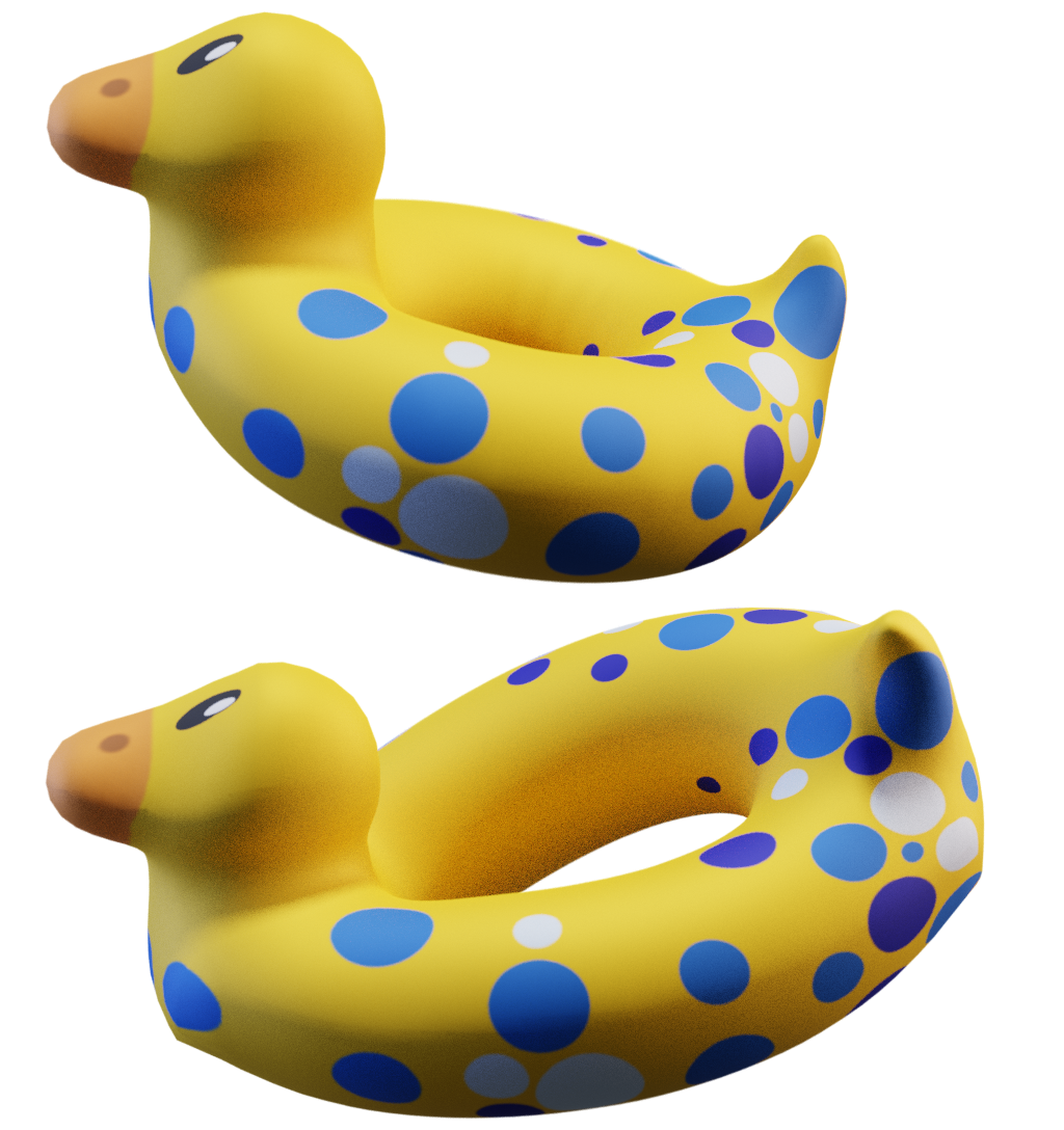
(c) Controlled deformation of the Bob model with incompressible neo-Hookean material by fixing the head and moving the tail. Top: rest shape. Bottom: deformed shape. Model created by Keenan Crane.

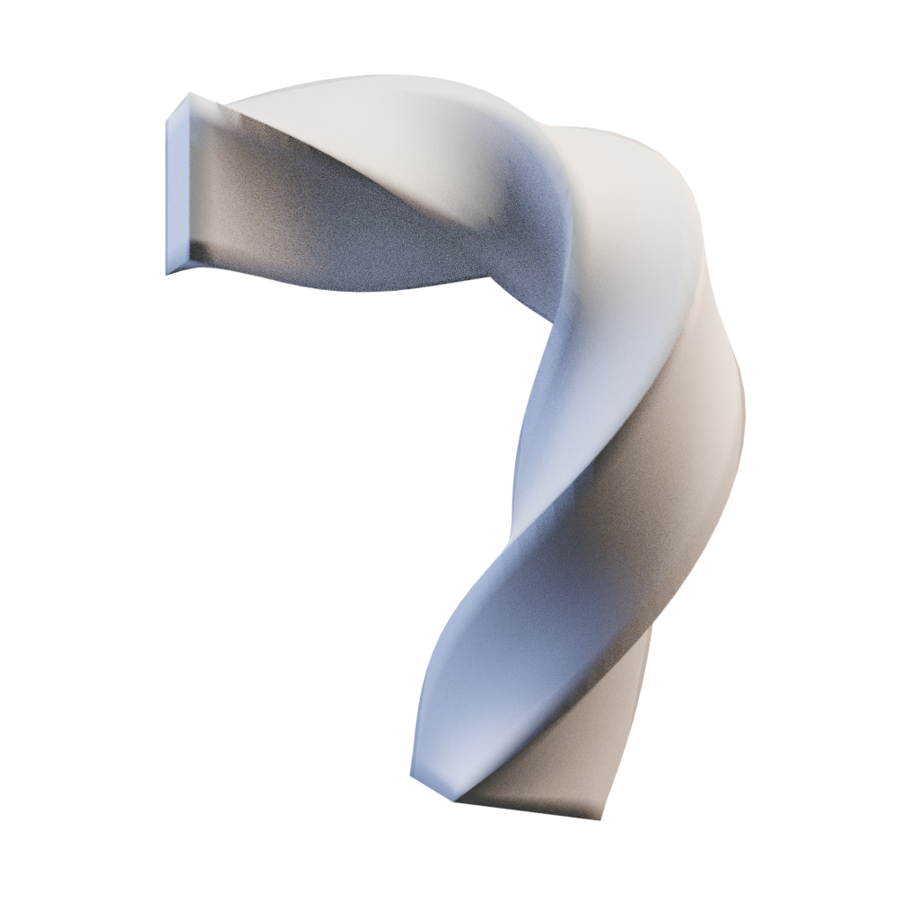
(d) Controlled deformation via twisting and bending a horozontal bar with the As-Rigid-As-Possible (ARAP) energy.

Figure 1. We present SANM, an open-source framework that automates and generalizes the Asymptotic Numerical Method (ANM) to solve symbolically represented nonlinear systems via numerical continuation and higher-order approximations. We apply SANM to static equilibrium problems via continuation on gravity (1(a) and 1(b)) and controlled mesh deformation problems with an implicit homotopy formulation via continuation on control handles (1(c) and 1(d)). SANM takes a symbolic representation of the nonlinear system from the user (Section 6) and automatically handles all the complexity of applying ANM.

1. Introduction

Solving nonlinear analytic systems (systems that can be locally described by a convergent power series) is at the core of many graphics and engineering applications. Such systems are traditionally solved with Newtonian methods that essentially use a first or second order local approximation. Newtonian methods converge quadratically fast when such an approximation is accurate enough, and the initial guess is sufficiently close. However, these assumptions are often violated in practice, and the convergence is thus much slower (Bonnans et al., 2006).

This paper considers solving the system $\bm{f}(\bm{x})+\bm{v}=\bm{0}$ under a numerical continuation framework (Allgower and Georg, 2003). Here $\bm{x}\in\mathbb{R}^{n}$ is an unknown vector, $\bm{f}:\mathbb{R}^{n}\mapsto\mathbb{R}^{n}$ is an analytic function, and $\bm{v}$ is a constant. Given an initial solution $\bm{x_{0}}$ such that $\bm{f}(\bm{x_{0}})=\bm{0}$, numerical continuation methods trace the final solution via solving $\bm{x}(\lambda)$ with $\lambda$ ranging from $0$ to $1$ subject to $\bm{f}(\bm{x}(\lambda))+\lambda\bm{v}=\bm{0}$. For example, in the static elasticity equilibrium problem, we encode the unknown node coordinates in $\bm{x}$, the mapping from node coordinates to node forces in $\bm{f}(\cdot)$, and the static external force in $\bm{v}$. By setting $\bm{x_{0}}$ as the rest shape, numerical continuation corresponds to gradually increasing the external force while simulating the deformation simultaneously. Figure 2 presents an example.

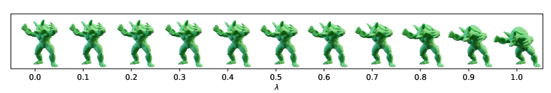
Figure 2. An example of solving gravity equilibrium with numerical continuation. Starting from an initial shape $\bm{x}(0)$, we solve $\bm{x}(\lambda)$ for $\lambda$ ranging from $0$ to $1$ subject to $\bm{f}(\bm{x}(\lambda))+\lambda\bm{g}=\bm{0}$ where $\bm{f}(\cdot)$ computes node elastic forces given node coordinates, and $\bm{g}$ is the per-node gravity vector. ANM parameterizes both $\bm{x}$ and $\lambda$ with $a$, and approximates $\bm{x}(a)$ and $\lambda(a)$ with power series. ANM allows easily computing the intermediate equilibrium states almost for free.

The Asymptotic Numerical Method (ANM) (Damil and Potier-Ferry, 1990) is a numerical continuation method that differs fundamentally from Newtonian approaches by exploring the landscape of the nonlinear system via higher-order approximations. The numerical continuation formulation $\bm{f}(\bm{x}(\lambda))+\lambda\bm{v}=\bm{0}$ defines a solution curve $(\bm{x}(\lambda),\,\lambda)$. However, parameterization of the curve using $\lambda$ can result in ill-conditioned behavior of $\bm{x}(\lambda)$. Instead, ANM parameterizes both $\bm{x}$ and $\lambda$ with $a$ such that $\bm{f}(\bm{x}(a))+\lambda(a)\bm{v}=\bm{0}$. ANM approximates the solution curve with a power series expansion at truncation order $N$: $\bm{x}(a)=\sum_{i=0}^{N}\bm{x_{i}}a^{i}$ and $\lambda(a)=\sum_{i=0}^{N}\lambda_{i}a^{i}$. Cochelin (1994) proposes a continuation technique to compute the final solution in a stepwise manner. Specifically, they estimate the valid range of the current approximation as $a_{r}$ and compute the final solution by iteratively recomputing the approximation at $\bm{x_{0}}=\bm{x}(a_{r})$ and $\lambda_{0}=\lambda(a_{r})$ until $\lambda(a_{r})$ reaches $1$.

Compared to the widely used Newtonian methods, ANM is able to determine a local representation of the solution curve with a larger range of validity in similar computing time (Cochelin et al., 1994b), and therefore solves the nonlinear system in fewer iterations and often less running time.

The core challenge in applying ANM is to solve the expansion coefficients $\{\bm{x_{i}}\}$ and $\{\lambda_{i}\}$. The original ANM framework (Damil and Potier-Ferry, 1990) analytically solves the coefficients for quadratic functions $\bm{f}(\bm{x})=\bm{x_{0}}+\bm{A}\bm{x}+\bm{x}^{\intercal}\bm{Q}\bm{x}$. Chen et al. (2014) deploys ANM on the inverse deformation problem for 3D fabrication by manually deriving the coefficient solution for the incompressible neo-Hookean elasticity (Bonet and Wood, 2008). They claim their Taylor coefficient derivation as a major contribution, which is a difficult and laborious task. They have also shown that ANM converges up to orders of magnitudes faster than Newtonian solvers.

To date, however, there is no scalable tool that automates the computation of Taylor coefficients in the general case. The lack of such tools severely limits the application of ANM to new problems. In this work, we show how to solve the coefficients $\{\bm{x_{i}}\}$ and $\{\lambda_{i}\}$ automatically and efficiently for a symbolically defined function $\bm{f}(\cdot)$. More specifically, we devise techniques to establish the connection of Taylor expansion coefficients between $\bm{x}(a)$ and $\quantity(\bm{f}\circ\bm{x})(a)$, which in fact conforms to an affine relationship for the highest-order term. We analyze a few operators important for graphics applications, including elementwise analytical functions (such as power and logarithm), matrix inverse, matrix determinant, and singular value decomposition. We speed up the system with batch computing that fits naturally into Finite Element Method (FEM) due to the same computation form shared by all quadrature points. We present a system, called SANM, as an implementation of our techniques.

We deploy SANM to solve the forward and inverse static force equilibrium problems similar to Chen et al. (2014). In contrast to their manual derivation that only works with incompressible neo-Hookean materials, our system allows easily solving more constitutive models by changing a few lines of code, including the compressible neo-Hookean model that has a logarithm term and the As-Rigid-As-Possible energy that involves a polar decomposition. Our experimental results show that SANM achieves comparable or better performance as the hand-coded, specialized ANM solver of Chen et al. (2014). We are unaware of efficient alternative methods for the inverse problem other than ANM. For the forward problem, an alternative is to minimize the total potential energy, and we show that SANM exhibits better performance than Newtonian energy minimizers.

We further extend the ANM framework to incorporate implicit homotopy $\bm{H}(\bm{x},\,\lambda)=\bm{0}$ where $\bm{H}:\mathbb{R}^{n+1}\mapsto\mathbb{R}^{n}$ admits a one-dimensional solution curve. For instance, we formulate the controlled mesh deformation as an implicit homotopy problem, defined as $\bm{H}(\bm{x},\,\lambda)=\bm{f}([\bm{x};\;\bm{x}_{c}+\lambda\bm{\Delta}_{x}])$, where $\bm{x}_{c}$ corresponds to the initial location of control handles, $\bm{\Delta}_{x}$ describes their user-specified movement, and $\bm{f}(\cdot)$ computes the internal elastic force. The coordinates of unconstrained nodes in the deformed equilibrium state, denoted by $\bm{x}^{*}$, are then governed by $\bm{H}(\bm{x}^{*},\,1)=\bm{0}$ and can be solved by continuation on $\lambda$. In our experiments, SANM runs 1.41 times faster by geometric mean than Newtonian energy minimization methods. We also demonstrate the robustness and versatility of SANM by twisting and bending a bar to extreme poses, as shown in Figure 1(d). Note that ANM and Newtonian minimization methods target different problems and can not replace each other. Section 7.3 further discusses their differences.

To summarize, this paper makes the following contributions:

1. We devise analytical solutions for Taylor coefficient propagation through a few nonlinear operators on which ANM has not been applied, including singular value decomposition as a challenging case (Section 5).

2. We present a system, SANM, that automatically solves the Taylor expansion coefficients for symbolically defined functions (Section 4). SANM greatly reduces programming effort for adopting ANM-based methods (Section 6.1). SANM adopts generic and FEM-specific optimizations to improve solving efficiency further.

3. We present a novel continuation algorithm to reduce accumulated numerical error and approximation error when solving the equational form $\bm{f}(\bm{x})+\bm{v}=\bm{0}$ (Section 4.3).

4. We extend ANM to handle implicit homotopy and apply it to controlled mesh deformation problems (Section 7.2). Our experiments show that SANM often converges faster than a state-of-the-art Newtonian energy minimizer. Moreover, the numerical continuation framework of SANM directly handles constitutive models that do not support inverted tetrahedrons, which would be challenging for energy minimization methods due to undefined elastic energy at the initial guess.

SANM is available at https://github.com/jia-kai/SANM.

2. Related Work

Numerical Optimization:

Numerical optimization has been extensively studied, and it is closely related to solving nonlinear systems. For example, we can recast solving $\bm{f}(\bm{x})=\bm{0}$ as minimizing $g(\bm{x})=\bm{f}(\bm{x})^{\intercal}\bm{f}(\bm{x})$ and apply generic minimization methods such as the Levenberg–Marquardt algorithm. On the other hand, minimizing $f(\bm{x})$ can often be approached via solving $\bm{\nabla}f(\bm{x})=\bm{0}$. For controlled mesh deformation problems, the internal elastic force corresponds to the gradient of the elastic potential energy with respect to node locations. Therefore, one can either directly solve a force equilibrium under Dirichlet boundary conditions (as done by SANM) or minimize the total potential energy to obtain the deformed state. We review the development of As-Rigid-As-Possible (ARAP) energy minimization as an example of improvements on numerical optimizers. Sorkine and Alexa (2007) devises a surface modeling technique by minimizing the ARAP energy via alternating between fitting the rotations and optimizing the locations. Chao et al. (2010) employs a Newton trust region solver to minimize the ARAP energy. Shtengel et al. (2017) accelerates the convergence by computing a positive semidefinite Hessian via constructing a convex majorizer for a specific class of convex-concave decomposable objectives, including the 2D ARAP energy. Smith et al. (2019) presents analytical solutions for the eigensystems of isotropic distortion energies to enable easily projecting the Hessians of 2D and 3D ARAP energies to be positive semidefinite to speed up the convergence. Most optimization methods inherently build on the classic idea of using first or second order approximations and exploit problem-specific optimization opportunities. This work targets generic nonlinear solving with numerical continuation and uses higher-order approximation.

Mesh Deformation:

Mesh deformation control is an important and widely studied problem in graphics. For animation production that only requires plausible but not physically accurate results, the simulation performance can be improved by a variety of approaches such as model analysis (Choi and Ko, 2005; Kim and James, 2009), skinning (Gilles et al., 2011), and constraint projection (Bender et al., 2014; Bouaziz et al., 2014). For physically predictive simulations, we need to stick to the formulation derived from continuum mechanics strictly, and the solver convergence rate is often improved by Hessian modification (Shtengel et al., 2017; Kim and Eberle, 2020). In this paper, we choose physically accurate elastic deformation as our target application. We approach the problem by solving a nonlinear system that encodes force equilibrium constraints.

Numerical Continuation Methods:

Classic numerical continuation methods include the predictor-corrector method and the piecewise-linear method. Allgower and Georg (2003) provides an introduction to this topic. The basic idea, which is to follow a solution trajectory by taking small steps, has become popular in many applications such as motion planning (Yin et al., 2008; Duenser et al., 2020), MRI reconstruction (Trzasko and Manduca, 2008), and drawing assistance (Limpaecher et al., 2013). These works typically choose a fixed step size or adopt a problem-specific step size schedule in the predictor and use classic first or second order solvers as the corrector. By contrast, asymptotic numerical methods use a higher-order approximation as the predictor without needing a corrector and adaptively choose the step size according to how well the predictor approximates the system.

Asymptotic Numerical Methods:

ANM has been applied to solve engineering problems in different domains, including buckling analysis (Azrar et al., 1993; Boutyour et al., 2004), vibration analysis (Azrar et al., 2002; Daya and Potier-Ferry, 2001), shell and rod simulation (Zahrouni et al., 1999; Lazarus et al., 2013), and inverse deformation problems (Chen et al., 2014). ANM assumes a quadratic system. An improvement over the standard ANM framework is to increase the range of validity of the approximation via imposing heuristics on the function behavior, such as replacing the power series with a Padé representation (Najah et al., 1998; Cochelin et al., 1994a; Elhage-Hussein et al., 2000). When adapting ANM to new problems, one typically needs to recast their specific problems into quadratic forms by introducing auxiliary variables and deriving the expansions manually (Guillot et al., 2019). Abichou et al. (2002) presents a review on adapting ANM for a few nonlinear functions.

Few attempts have been made to automate ANM to handle general nonlinearities. Notably, Charpentier et al. (2008) proposes an automatic differentiation framework, called Diamant, that computes the expansion coefficients by Taylor coefficient propagation via computing higher-order derivatives of the operators. Unfortunately, the Diamant approach is not readily applicable to mesh deformation problems due to the difficulty in computing higher-order derivatives of certain matrix functions such as matrix inverse or determinant used in the constitutive models. Moreover, Diamant is not designed with high-performance computing in mind. It only works with scalar variables, does not take advantage of the structural sparsity in FEM problems, and is only evaluated on small-sized problems. Lejeune et al. (2012) incorporates the Diamant approach into an object-oriented solver to automate ANM. By contrast, SANM natively works with multidimensional variables and is accelerated with batch computing for large-scale FEM problems. SANM also implements a generic framework for computing the expansion coefficients, which is not limited to the higher-order derivative approach of Diamant and is capable of handling challenging matrix functions.

3. ANM Background

This section introduces the asymptotic numerical method. We begin with a toy example of a geometry problem and then formally describe ANM. We first define the notations used in this paper in Table 1.

Table 1. Notation definition

$f$, $x$	Scalars or scalar-valued functions
$\bm{f}$, $\bm{x}$	Vectors or vector-valued functions
$f_{i}$, $x_{i}$	A scalar in the vector at given index. For a function $f(\cdot)$, we also use $f_{i}$ to represent its $i^{\text{th}}$ Taylor coefficient, and similarly for $\bm{f}(\cdot)$ vs $\bm{f_{i}}$ and $\bm{F}(\cdot)$ vs $\bm{F_{i}}$.
$\bm{f_{i}}$, $\bm{x_{i}}$	A vector in an array of vectors
$\bm{F}$, $\bm{X}$	Matrices or matrix-valued functions
$\bm{F_{i}}$, $\bm{X_{i}}$	A matrix in an array of matrices
$X_{ij}$	A coefficient in the matrix at given row and column
$\bm{X}_{\mathchoice{\mathbin{\vbox{\hbox{\scalebox{0.5}{$\displaystyle\bullet$}}}}}{\mathbin{\vbox{\hbox{\scalebox{0.5}{$\textstyle\bullet$}}}}}{\mathbin{\vbox{\hbox{\scalebox{0.5}{$\scriptstyle\bullet$}}}}}{\mathbin{\vbox{\hbox{\scalebox{0.5}{$\scriptscriptstyle\bullet$}}}}}i}$, $\bm{X}_{j\mathchoice{\mathbin{\vbox{\hbox{\scalebox{0.5}{$\displaystyle\bullet$}}}}}{\mathbin{\vbox{\hbox{\scalebox{0.5}{$\textstyle\bullet$}}}}}{\mathbin{\vbox{\hbox{\scalebox{0.5}{$\scriptstyle\bullet$}}}}}{\mathbin{\vbox{\hbox{\scalebox{0.5}{$\scriptscriptstyle\bullet$}}}}}}$	The vectors corresponding to the $i^{\text{th}}$ row or the $j^{\text{th}}$ column in matrix $\bm{X}$
$\operatorname{RMS}(\bm{x})$	Root-mean-square of $\bm{x}\in\mathbb{R}^{n}$: $\operatorname{RMS}(\bm{x})=\sqrt{\nicefrac{{\bm{x}^{\intercal}\bm{x}}}{{n}}}$
$\operatorname{vec}(\bm{X})$	Flatten a matrix $\bm{X}$ into a column vector by concatenating the columns in $\bm{X}$
$\norm{\bm{X}}$	Frobenius norm of the matrix $\bm{X}$, defined as $\sqrt{\operatorname{vec}(\bm{X})^{\intercal}{\operatorname{vec}(\bm{X})}}$
$\operatorname{diag}(\bm{X})$	A vector containing the diagonal coefficients of $\bm{X}$
$o(x)$	The little-o notation: $y=o(x)$ if $\nicefrac{{y}}{{x}}\to 0$.

3.1. A Circle-ellipse Intersection Problem

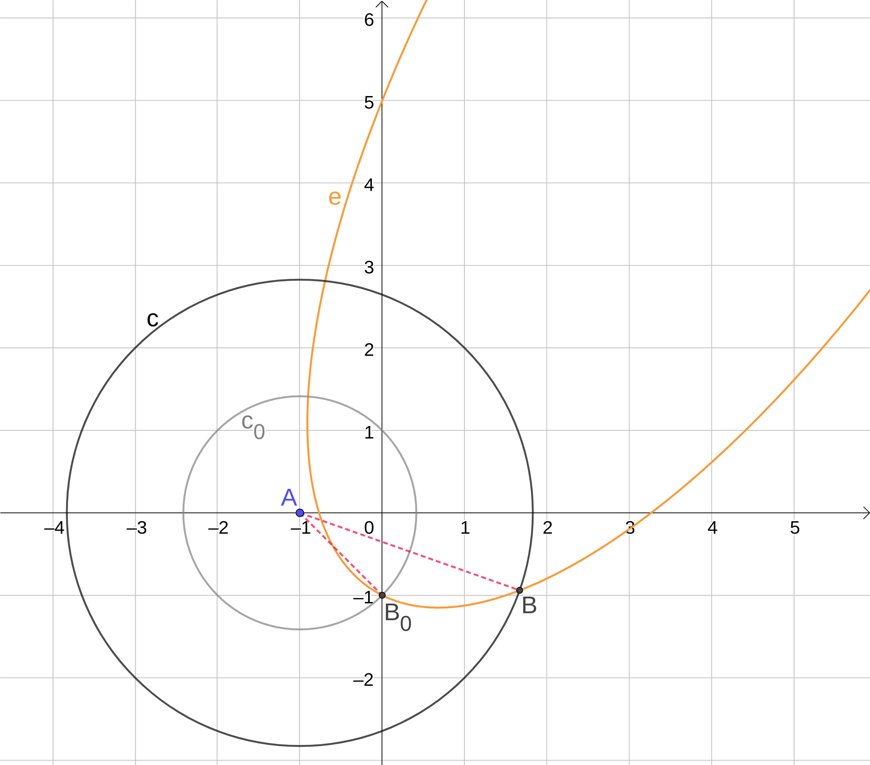
Figure 3. Our circle-ellipse intersection example problem. ANM uses polynomials to approximate the trace of intersection points between the ellipse and concentric circles of radius from $\sqrt{2}$ to $\sqrt{8}$, which is the arc $\wideparen{\bm{B_{0}}\bm{B}}$.

We illustrate ANM with a toy problem that asks for the intersection $\bm{B}$ of an ellipse $e$ and a circle $c$ as shown in Figure 3. The ellipse intersects the y-axis at $\bm{B_{0}}=(0,\,-1)$. The circle is centered at $A=(-1,\,0)$ and its radius is $|\bm{A}\bm{B}|=\sqrt{8}$. To solve the problem with ANM, we first choose a continuation scheme. We start with a smaller concentric circle $c_{0}$ with radius $|\bm{A}\bm{B_{0}}|=\sqrt{2}$ and continuously trace its intersection with $e$ while increasing its radius from $\sqrt{2}$ to $\sqrt{8}$. Note that the continuation scheme is problem-specific. While there can be many choices, practical problems typically admit a “natural” choice, such as the external force in static equilibrium problems.

Formally, our goal is to solve $(x,\,y)$ such that $f_{e}(x,\,y)=f_{c}(x,\,y)=0$, where $f_{e}(\cdot)$ and $f_{c}(\cdot)$ describe the ellipse $e$ and the circle $c$ respectively:

(3) $$\begin{array}[]{rl}f_{e}(x,\,y)=&2x^{2}-5x+y^{2}-4y-2xy-5\\ f_{c}(x,\,y)=&(x+1)^{2}+y^{2}-8\end{array}$$

ANM introduces a variable $\lambda\in[0,\,1]$ to represent the continuation. ANM traces the solution curve starting at $(x_{0},\,y_{0})$ via varying $\lambda$ from $0$ to $1$ while keeping the following equations satisfied:

(7) $$\begin{array}[]{rl}f_{e}(x,\,y)&=0\lambda\\ f_{c}(x,\,y)+6&=6\lambda\\ (x_{0},\,y_{0})&=\bm{B_{0}}=(0,\,-1)\end{array}$$

Geometrically, ANM continuously solves the intersection between the ellipse and a concentric circle with radius $\sqrt{2+6\lambda}$. ANM parameterizes the solution curve by a variable $a$ and approximates $x(a)$, $y(a)$, and $\lambda(a)$ with polynomial expansions at truncation order $N$, with coefficients $\{x_{k}\}$, $\{y_{k}\}$, and $\{\lambda_{k}\}$ to be solved:

(11) $$\begin{array}[]{rl}x(a)&=0+\sum_{k=1}^{N}x_{k}a^{k}\\ y(a)&=-1+\sum_{k=1}^{N}y_{k}a^{k}\\ \lambda(a)&=0+\sum_{k=1}^{N}\lambda_{k}a^{k}\\ \end{array}$$

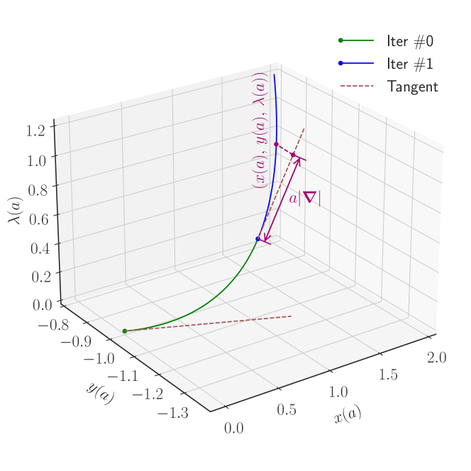
Figure 4. ANM solution curve for the circle-ellipse intersection problem. ANM solves the problem in two iterations. The path parameter $a$ is identified by the projection of a point $(x(a),\,y(a),\,\lambda(a))$ onto the tangent direction. The length of the projection is $a|\bm{\nabla}|$ where $\bm{\nabla}=(x^{\prime}(0),\,y^{\prime}(0),\,\lambda^{\prime}(0))$ is the gradient at the beginning of the current iteration.

We iteratively solve the coefficients by introducing the lower-order terms in (11) into (7). We start with $(x_{1},\,y_{1},\,\lambda_{1})$ and introduce $x=x_{1}a$, $y=-1+y_{1}a$, and $\lambda=\lambda_{1}a$ into (7):

(14) $$\begin{array}[]{rll}f_{e}(x_{1}a,\,y_{1}a-1)&=-(3x_{1}+6y_{1})a+o(a)&=0\\ f_{c}(x_{1}a,\,y_{1}a-1)+6&=(2x_{1}-2y_{1})a+o(a)&=6\lambda_{1}a\\ \end{array}$$

We obtain two linear constraints on the three unknowns by equating the coefficient of $a$ in (14). Let $\bm{u}(a)=[x(a);\;y(a);\;\lambda(a)]$ denote the solution curve. ANM further identifies the path parameter $a$ as the pseudo-arclength that is the projection of the path along its tangent direction as shown in Figure 4, specifically $a=\quantity(\bm{u}(a)-\bm{u}(0))^{\intercal}\bm{u}^{\prime}(0)$, which provides the third constraint for a full-rank system:

(18) $$\left\{\begin{array}[]{rl}-3x_{1}-6y_{1}&=0\\ 2x_{1}-2y_{1}-6\lambda_{1}&=0\\ x_{1}^{2}+y_{1}^{2}+\lambda_{1}^{2}&=1\end{array}\right.$$

We require $\lambda_{1}$ to be positive so that $\lambda(a)$ is a locally increasing function at $0$, and the solution of (18) is $x_{1}=\nicefrac{{2}}{{\sqrt{6}}}$, $y_{1}=-\nicefrac{{1}}{{\sqrt{6}}}$, and $\lambda_{1}=\nicefrac{{1}}{{\sqrt{6}}}$. We then solve $(x_{2},\,y_{2},\,\lambda_{2})$ by equating the coefficients of $a^{2}$ in $f_{e}(x_{2}a^{2}+\nicefrac{{2}}{{\sqrt{6}}}a,\,y_{2}a^{2}-\nicefrac{{1}}{{\sqrt{6}}}a-1)=0$ and $f_{c}(x_{2}a^{2}+\nicefrac{{2}}{{\sqrt{6}}}a,\,y_{2}a^{2}-\nicefrac{{1}}{{\sqrt{6}}}a-1)=6(\lambda_{2}a^{2}+\nicefrac{{1}}{{\sqrt{6}}}a)$. Expanding the equations results in two linear constraints for the three unknowns. The third pseudo-arclength constraint is $x_{1}x_{k}+y_{1}y_{k}+\lambda_{1}\lambda_{k}=0$ for $k\geq 2$. Repeating this step, we can solve the coefficients $\{x_{k}\}$, $\{y_{k}\}$, and $\{\lambda_{k}\}$ that define the polynomials $x(a)$, $y(a)$, and $\lambda(a)$. As will be shown in Section 3.3, the equations for all $(x_{k},\,y_{k},\,\lambda_{k})$ are linear, and the coefficients in these equations are the gradients of $f_{e}(\cdot)$ and $f_{c}(\cdot)$ evaluated at $(x_{0},\,y_{0})$.

We then estimate $a_{r}$, the range of validity of the polynomial approximations $x(a)$, $y(a)$, and $\lambda(a)$. We iteratively compute a new approximation at $(x(a_{r}),\,y(a_{r}))$ to extend the solution curve until $\lambda(a_{r})\geq 1$, and we compute the final solution $(x(a^{*}),\,y(a^{*}))$ with $a^{*}=\lambda^{-1}(1)$. ANM with truncation order $N=20$ is able to find the circle-ellipse intersection with a residual (defined as $\sqrt{\nicefrac{{\quantity(f_{e}^{2}(\bm{x})+f_{c}^{2}(\bm{x}))}}{{2}}}$) of $2\times 10^{-6}$ in two iterations. Figure 4 visualizes the parametric solution curve. The continuation formulation presented in Section 4.3 further reduces the residual to $7\times 10^{-9}$.

An alternative is the Newton-Raphson method, which iteratively computes $\bm{x_{n+1}}=\bm{x_{n}}-\bm{J}(\bm{x_{n}})^{-1}\bm{f}(\bm{x_{n}})$, where $\bm{f}(\bm{x})=[f_{e}(\bm{x});\;f_{c}(\bm{x})]$ and $\bm{J}(\bm{x})$ is the Jacobian of $\bm{f}$ evaluated at $\bm{x}$. Starting at $\bm{x_{0}}=(0,\,-1)$, the Newton-Raphson method needs four evaluations of the Jacobian to converge to a solution with a residual of $8\times 10^{-5}$.

3.2. ANM Overview

ANM aims to solve the nonlinear system $\bm{f}(\bm{x})+\bm{v}=\bm{0}$ with numerical continuation, where $\bm{f}:\mathbb{R}^{n}\mapsto\mathbb{R}^{n}$ is an analytic function, and $\bm{v}$ is a constant. Starting from an initial solution $(\bm{x_{0}},\,\lambda_{0})$ such that $\bm{f}(\bm{x_{0}})+\lambda_{0}\bm{v}=\bm{0}$, continuation methods compute an approximation to trace the nearby solution curve of $\bm{f}(\bm{x})+\lambda\bm{v}=\bm{0}$. In the general case, the curve may not be well-conditioned under the parameterization with respect to $\lambda$, and it is preferable to consider an arclength parameterization $\bm{x}(a)$ and $\lambda(a)$ where $a$ measures the arclength or pseudo-arclength (Allgower and Georg, 2003).

ANM approximates $\bm{x}(a)$ and $\lambda(a)$ by Taylor expansion at truncation order $N$ such that $\bm{f}(\bm{x}(a))+\lambda(a)\bm{v}$ should be sufficiently close to zero for small values of $a$:

(22) $$\begin{array}[]{rl}\bm{x}(a)&=\sum_{i=0}^{N}\bm{x_{i}}a^{i}\\ \lambda(a)&=\sum_{i=0}^{N}\lambda_{i}a^{i}\\ \text{s.t. }&\norm{\bm{f}(\bm{x}(a))+\lambda(a)\bm{v}}=o(a^{N})\end{array}$$

We require $\lambda_{1}>0$ so that $\lambda(a)$ is locally increasing, and the algorithm makes progress. We then estimate the range of validity $a_{r}$ such that $\bm{x}(a)$ and $\lambda(a)$ are good approximations of the solution when $|a|<a_{r}$. If $\lambda(a_{r})\geq 1$, we can solve $a^{*}$ such that $\lambda(a^{*})=1$ and compute the final solution $x^{*}=\bm{x}(a^{*})$. Otherwise, when $\lambda(a_{r})<1$, we recompute the power series approximation starting at $\bm{x_{0}}=\bm{x}(a_{r})$ and $\lambda_{0}=\lambda(a_{r})$ and repeat the above steps.

A simple method to estimate $a_{r}$, as suggested by Cochelin (1994), builds on the idea that within the range of validity, different orders of approximation should behave similarly:

(23) $$\frac{\norm{\bm{x}(a)_{\text{order $N$}}-\bm{x}(a)_{\text{order $N-1$}}}}{\norm{\bm{x}(a)_{\text{order $N$}}-\bm{x_{0}}}}<\epsilon$$

which leads to an approximation

(24) $$a_{r}\approx\quantity(\epsilon\frac{\norm{\bm{x_{1}}}}{\norm{\bm{x_{N}}}})^{\frac{1}{N-1}}$$

The equation $\lambda(a^{*})=1$ can be solved by a univariate polynomial root finding algorithm such as Brent’s method (Brent, 2013).

The remaining part of completing the ANM algorithm is to solve the coefficients $\{\bm{x_{i}}\}$ and $\{\lambda_{i}\}$ efficiently, which is a core contribution of this paper.

We solve the coefficients $\{\bm{x_{i}}\}$ and $\{\lambda_{i}\}$ iteratively. Assume we are at the $k^{\text{th}}$ iteration, where $\{\bm{x_{0}},\ldots,\bm{x_{k-1}}\}$ and $\{\lambda_{0},\,\ldots,\,\lambda_{k-1}\}$ have been solved. With $\bm{x_{k}}\in\mathbb{R}^{n}$ and $\lambda_{k}\in\mathbb{R}$ currently unknown, we have the equation:

(25) $$\bm{f}(\bm{x}(a)))+\lambda(a)\bm{v}\approx\bm{f}\quantity(\sum_{i=0}^{k}\bm{x_{i}}a^{i})+\quantity(\sum_{i=0}^{k}\lambda_{i}a^{i})\bm{v}\approx\bm{0}$$

Assume $\{\bm{f_{i}}\}$ are the Taylor coefficients of $\bm{f}(\bm{x}(a))$:

(26) $$\bm{f}(\bm{x}(a))\approx\bm{f}\quantity(\sum_{i=0}^{k}\bm{x_{i}}a^{i})=\sum_{i=0}^{k}\bm{f_{i}}a^{i}+o(a^{k})$$

As will be shown in 1, for an analytic function $\bm{f}(\cdot)$, there is an affine relationship between $\bm{f_{k}}$ and $\bm{x_{k}}$, specifically $\bm{f_{k}}=\bm{P}(\bm{x_{0}})\bm{x_{k}}+\bm{q}(\bm{x_{0}},\ldots,\bm{x_{k-1}})$, where $\bm{P}(\bm{x_{0}})\in\mathbb{R}^{n\times n}$ is the slope matrix and $\bm{q}(\cdot)\in\mathbb{R}^{n}$ is the bias vector. By introducing this relationship into the original equation and requiring the coefficient of $a^{k}$ to be zero, we obtain a linear system that restricts $\bm{x_{k}}$ and $\lambda_{k}$:

(27) $$\bm{P}(\bm{x_{0}})\bm{x_{k}}+\lambda_{k}\bm{v}=-\bm{q}(\bm{x_{0}},\,\ldots,\,\bm{x_{k-1}})$$

However, the system has rank $n$ but there are $n+1$ unknowns because the curve behavior with respect to its parameter $a$ is not fully constrained. To obtain a full rank system, Cochelin (1994) proposes to identify the path parameter $a$ as the pseudo-arclength, similar to other numerical continuation methods (Allgower and Georg, 2003). Pseudo-arclength approximates the arclength of a curve by projecting it onto the tangent space, which constitutes the following constraint:

(28) $$a=(\bm{x}(a)-\bm{x_{0}})^{\intercal}\bm{x^{\prime}}(0)+(\lambda(a)-\lambda_{0})\lambda^{\prime}(0)$$

Introduce (22) into (28):

(29) $$\bm{x_{i}}^{\intercal}\bm{x_{1}}+\lambda_{i}\lambda_{1}=\mathbbm{1}_{i=1}$$

The unknowns $\bm{x_{k}}$ and $\lambda_{k}$ can be solved by combining (27) and (29). The solution is unique if we further require $\lambda^{\prime}(0)=\lambda_{1}>0$.

3.3. Linearity Between Taylor Coefficients

Before proving the linearity between $\bm{f_{k}}$ and $\bm{x_{k}}$ in (26), we introduce an auxiliary definition:

Definition 0.

Define $\mathfrak{C}_{a}^{(k)}\left[f(a)\right]$ to be the coefficient of $a^{k}$ in the Taylor expansion of an analytic function $f:\mathbb{R}\mapsto\mathbb{R}$ such that:

$$f(a)=\sum_{i\geq 0}\mathfrak{C}_{a}^{(i)}\left[f(a)\right]a^{i}$$

Proposition 1.

Let $f:\mathbb{R}^{n}\mapsto\mathbb{R}$ be an analytic function, and $\bm{x_{0}},\,\ldots,\,\bm{x_{k-1}}$ known real-valued $n$-dimensional vectors. Assume coefficients $f_{0},\,\ldots,\,f_{k}$ satisfy:

$$f\quantity(\sum_{i=0}^{k}\bm{x_{i}}a^{i})=\sum_{i=0}^{k}f_{i}a^{i}+o\quantity(a^{k})$$

Then we have $f_{k}=\bm{p}(\bm{x_{0}})^{\intercal}\bm{x_{k}}+\bm{q}(\bm{x_{0}},\,\ldots,\,\bm{x_{k-1}})$. Specifically, $\bm{p}(\bm{x_{0}})=\gradient{f}(\bm{x_{0}})$ and $\bm{q}(\bm{x_{0}},\,\ldots,\,\bm{x_{k-1}})=\mathfrak{C}_{a}^{(k)}\left[f\left(\sum_{i=0}^{k-1}\bm{x_{i}}a^{i}\right)\right]$.

Proof.

We prove the univariate case for the simplicity of the notations. Our argument also applies to multivariate functions by using the multivariate Taylor theorem.

Let $g(t)=f(x_{0}+t)=\sum_{i\geq 0}g_{i}t^{i}$ where $g_{i}=\frac{1}{i!}\evaluated{\derivative[i]{g}{t}}_{t=0}$ is the Taylor expansion coefficient and $g_{0}=f_{0}=f(x_{0})$. With $t=\sum_{i=1}^{k}x_{i}a^{i}$, we rewrite

$$f\quantity(\sum_{i=0}^{k}x_{i}a^{i})=g\quantity(\sum_{i=1}^{k}x_{i}a^{i})=g_{0}+\sum_{i\geq 1}g_{i}\quantity(\sum_{j=1}^{k}x_{j}a^{j})^{i}$$

To compute $f_{k}$, we consider the terms that contribute to $a^{k}$ in the expansion of the right side hand:

1. For terms that contain $x_{k}$ and contribute to $f_{k}$, it must contain $x_{k}a^{k}$ and no other $x_{i}a^{i}$ for which $i>0$. There is only one such term, which is $g_{1}x_{k}a^{k}$. The slope $p$ for which $f_{k}=px_{k}+q$ is thus $p=g_{1}=f^{\prime}(x_{0})$.

2. The bias $q$ consists of terms that do not contain $x_{k}$, which can be computed by treating $x_{k}$ as zero, or equivalently removing $x_{k}a^{k}$ from $t$:

   $$q=\mathfrak{C}_{a}^{(k)}\left[f\quantity(\sum_{i=0}^{k-1}x_{i}a^{i})\right]$$

∎

Remarks:

We have discussed the case of scalar functions. For a vector function $\bm{f}:\mathbb{R}^{n}\mapsto\mathbb{R}^{m}$, the slope matrix $\bm{P}$ is its Jacobian. Note that $\bm{p}(\bm{x_{0}})$ only depends on the initial point $\bm{x_{0}}$ and remains constant for all orders. This allows us to factorize the coefficient matrix only once to solve all the terms. The result of 1 is not new. For example, it is a direct consequence of Faà di Bruno’s formula (Roman, 1980). Here we have presented a simple proof based on elementary calculus.

3.4. Continuation with Padé Approximation

The original ANM approximates $\bm{x}(a)$ and $\lambda(a)$ with Taylor expansions. It has been shown that replacing the Taylor expansions with Padé approximations results in a larger range of validity and thus fewer iterations.

For a scalar function $f:\mathbb{R}\mapsto\mathbb{R}$, its Padé approximation of order $M+N$ approximates the function with a ratio of two polynomials, $P_{N}(x)$ and $Q_{M}(x)$ of degrees $N$ and $M$, respectively, such that $f(x)=\frac{P_{N}(x)}{Q_{M}(x)}+o(x^{N+M})$. The polynomials $P_{N}(x)$ and $Q_{M}(x)$ are determined by the first $N+M+1$ Taylor coefficients of $f$ via a set of linear constraints up to a common scaling factor. Although the Padé approximation is constructed from the information contained in the Taylor expansion, for many functions, it has a larger range of validity than the Taylor series, and it sometimes gives meaningful results even when the radius of convergence of the Taylor series is strictly zero (Basdevant, 1972).

Cochelin et al. (1994a) proposes to construct a Padé approximation for the vector function $\bm{x}(a)=\sum_{i=0}^{N}\bm{x_{i}}a^{i}$ in the form:

$$\bm{P}_{N}(a) =\bm{x_{0}}+\sum_{i=1}^{N-1}\frac{D_{N-1-i}(a)}{D_{N-1}(a)}\bm{x_{i}}a^{i}$$

(30) $$D_{k}(a) =\sum_{i=0}^{k}d_{i}a^{i}$$

Najah et al. (1998) presents the process of computing the coefficients $\{d_{i}\}$ from $\{\bm{x_{i}}\}$, which first orthonormalizes $\{\bm{x_{i}}\}$ and then solves $\{d_{i}\}$ based on the principle that the Padé approximation should share the same lower-order Taylor coefficients. We omit the details here.

We follow the techniques presented in Elhage-Hussein et al. (2000) to determine the range of validity $a_{p}$ for this Padé approximation:

(31) $$\frac{\norm{P_{N}(a_{p})-P_{N-1}(a_{p})}}{\norm{P_{N}(a_{p})-P_{N}(0)}}<\epsilon$$

The number $a_{p}$ is sought via bisection in the range $(a_{r},r)$, where $a_{r}$ is the range of validity of the Taylor series determined by (24), and $r$ is the smallest positive real root of $D_{N-1}(a)$ that can be found by numerical methods such as Bairstow algorithm (Golub and Robertson, 1967). Note that $P_{N-1}$ is not the first $N-1$ terms in $P_{N}$ but the Padé approximation computed from $\{\bm{x_{0}},\,\ldots,\,\bm{x_{N-1}}\}$. For all the 36 test cases presented in Section 7, Padé approximation uses $1.14\pm 0.57$ fewer iterations than the original ANM formulation on average.

4. The SANM Framework

This section presents the overall design of SANM and its two novel extensions over ANM: the handling of implicit homotopy $\bm{H}(\bm{x},\,\lambda)=\bm{0}$ and a formulation to reduce accumulated error when solving the equational form $\bm{f}(\bm{x})+\bm{v}=\bm{0}$. Note that this paper deals with both computing graphs and mesh networks. We use vertex to refer to a vertex in a graph and node to refer to a node in a polygon mesh.

4.1. Coefficient Propagation on the Computing Graph

Algorithm 1 Taylor coefficient solver in SANM

Input: Computing graph $G=(V_{o}\cup V_{v},\,E)$

          that represents $\bm{H}:\mathbb{R}^{n+1}\mapsto\mathbb{R}^{n}$

Input: Initial value $\bm{x_{0}}\in\mathbb{R}^{n}$ and $\lambda_{0}\in\mathbb{R}$ such that $\bm{H}(\bm{x_{0}},\,\lambda_{0})=\bm{0}$

Input: Truncation order $N$

Output: Taylor coefficients $\{\bm{x_{i}}\}$ and $\{\lambda_{i}\}$ such that

          $\norm{\bm{H}\quantity(\sum_{i=0}^{N}\bm{x_{i}}a^{i},\,\sum_{i=0}^{N}\lambda_{i}a^{i})}=o(a^{N})$

Compute $\bm{P}\leftarrow\partialderivative{\bm{H}}{\bm{x}}\/(\bm{x_{0}},\,\lambda_{0})$ by reverse mode AD on $G$

Meanwhile, record the Jacobians $\bm{p^{u}}$ for each operator $u\in V_{o}$

Meanwhile, record $\bm{v}\leftarrow\partialderivative{\bm{H}}{\lambda}\/(\bm{x_{0}},\,\lambda_{0})$

Factorize $\bm{P}$

for $k\leftarrow 1$ to $N$ do

     Compute the biases $\bm{q_{k}^{u}}$ for $u\in V_{o}$ in topological order,

          given $\bm{x_{0}},\,\lambda_{0},\,\ldots,\,\bm{x_{k-1}},\,\lambda_{k-1}$ and the rules in Section 5

     Compute $\bm{q_{k}}$ by combining affine transformations $(\bm{p^{u}},\,\bm{q_{k}^{u}})$

          for $u\in V_{o}$ in topological order

     Solve $\bm{x_{k}}$ and $\lambda_{k}$ according to (29) and (33):

$$\left\{\begin{array}[]{l}\bm{P}\bm{x_{k}}+\lambda_{k}\bm{v}=-\bm{q_{k}}\\ \bm{x_{k}}^{\intercal}\bm{x_{1}}+\lambda_{k}\lambda_{1}=\mathbbm{1}_{k=1}\end{array}\right.$$

end for

SANM represents a nonlinear function $\bm{f}(\cdot)$ as a directed acyclic bipartite computing graph composed of predefined operators: $G=(V_{o}\cup V_{v},\,E)$. The user builds the graph to specify the nonlinear function in their problem symbolically. The vertex set $V_{o}$ corresponds to a subset of predefined operators offered by SANM: for $u\in V_{o}$, there is a function $f_{u}$ that defines the corresponding computing. Each operator takes a fixed number of inputs, where each input can be a higher-order tensor. For example, matrix inverse takes one matrix input, and vector addition takes two vector inputs. The vertex set $V_{v}$ represents the variables. For a variable $v\in V_{v}$ and an operator $u\in V_{o}$, an edge $(v,\,u)\in E$ if the user passes $v$ as an input of the function $f_{u}$. An edge $(u,\,v)\in E$ if $v$ is an output of the function $f_{u}$. Many successful symbolic-numerical systems, such as Theano (Theano Development Team, 2016) and Tensorflow (Abadi et al., 2016), have adopted computing graphs to represent user-defined functions.

Besides working with the original ANM formulation $\bm{f}(\bm{x})+\lambda\bm{v}=\bm{0}$, SANM also supports solving the more general implicit homotopy: $\bm{H}(\bm{x},\,\lambda)=\bm{0}$. Implicit homotopy defines a curve $\bm{x}(\lambda)$. Our goal is to solve $\bm{x}(1)$ given an initial value $\bm{x}(0)$.

1 implies that the $k^{\text{th}}$ order expansion of the implicit homotopy can be written as:

(32) $$\bm{H}\quantity(\sum_{i=0}^{k}\bm{x_{i}}a^{i},\sum_{i=0}^{k}\lambda_{i}a^{i})=\sum_{i=0}^{k-1}\bm{H_{i}}a^{i}+\\ \quantity(\partialderivative{\bm{H}}{\bm{x}}\/(\bm{x_{0}},\,\lambda_{0})\cdot\bm{x_{k}}+\partialderivative{\bm{H}}{\lambda}\/(\bm{x_{0}},\,\lambda_{0})\cdot\lambda_{k}+\bm{q_{k}})a^{k}+\cdots$$

By requiring the coefficient of $a^{k}$ to be zero, we obtain the equation

(33) $$\partialderivative{\bm{H}}{\bm{x}}\/(\bm{x_{0}},\,\lambda_{0})\cdot\bm{x_{k}}+\partialderivative{\bm{H}}{\lambda}\/(\bm{x_{0}},\,\lambda_{0})\cdot\lambda_{k}+\bm{q_{k}}=\bm{0}$$

Given a user-defined function $\bm{H}(\cdot)$ and initial values $\bm{H}(\bm{x_{0}},\,\lambda_{0})=\bm{0}$, SANM computes the slope matrix $\bm{P}=\frac{\partial\bm{H}}{\partial\bm{x}}(\bm{x_{0}},\,\lambda_{0})$ via reverse mode Automatic Differentiation (AD) (Baydin et al., 2018). It then iteratively computes the biases for each order and solves the Taylor coefficients according to (29) and (33). The bias $\bm{q_{k}}$ is computed by merging the affine transformations of individual operators in $G$. Algorithm 1 summarizes this process.

4.2. Continuation in SANM

Algorithm 2 Continuation framework in SANM

Input: An analytic function $\bm{H}:\mathbb{R}^{n+1}\mapsto\mathbb{R}^{n}$

Input: Initial value $\bm{x_{0}}\in\mathbb{R}^{n}$ and $\lambda_{0}\in\mathbb{R}$ such that $\bm{H}(\bm{x_{0}},\,\lambda_{0})=\bm{0}$

Input: Target location of the homotopy $\lambda_{t}>\lambda_{0}$

Output: The solution $\bm{x^{*}}\in\mathbb{R}^{n}$ such that $\bm{H}(\bm{x^{*}},\,\lambda_{t})=\bm{0}$

$k\leftarrow 0$

while $\lambda_{k}<\lambda_{t}$ do

     Compute Taylor coefficients $\{\bm{x_{k,i}}\}$ and $\{\lambda_{k,i}\}$

          using Algorithm 1

     Compute the corresponding Padé approximation $P_{N}(a)$

     Compute $a_{r}$ and $a_{p}$, the range of validity

          for these two approximations

     $a_{m}\leftarrow\max(a_{r},\,a_{p})$

     Use Taylor or Padé to approximate $\bm{f_{x}}(a)$ and $f_{\lambda}(a)$,

          depending on which one achieves the range $a_{m}$

     Solve $a^{\prime}$ such that $f_{\lambda}(a^{\prime})=\min(f_{\lambda}(a_{m}),\,\lambda_{t})$

     $(\bm{x_{k+1}},\,\lambda_{k+1})\leftarrow(\bm{f_{x}}(a^{\prime}),\,f_{\lambda}(a^{\prime}))$

     $k\leftarrow k+1$

end while

$\bm{x^{*}}\leftarrow\bm{x_{k}}$

SANM aims to solve $\bm{x^{*}}$ such that $\bm{H}(\bm{x^{*}},\,\lambda_{t})=\bm{0}$ given initial values $\bm{H}(\bm{x_{0}},\,\lambda_{0})=\bm{0}$. We typically have $\lambda_{0}=0$ and $\lambda_{t}=1$. Note that we have changed the meaning of $\bm{x_{k}}$ and $\lambda_{k}$ to indicate the initial values at the $k^{\text{th}}$ iteration rather than the $k^{\text{th}}$ Taylor coefficient as in Section 4.1.

Similar to the standard ANM procedure, at the $k^{\text{th}}$ iteration, SANM uses Algorithm 1 to compute the local Taylor expansion coefficients of $\bm{x}(a)$ and $\lambda(a)$ near $(\bm{x_{k}},\,\lambda_{k})$ so that $\bm{H}(\bm{x}(a),\,\lambda(a))\approx\bm{0}$. SANM then estimates the range of validity $a_{r}$ using the standard ANM formulation in (24). SANM also computes a Padé approximation from the Taylor coefficients and estimates its range of validity $a_{p}$ using techniques outlined in Section 3.4. SANM chooses the approximation with a larger range of validity and computes the next approximation to extend the solution path until $\lambda(a)$ reaches $\lambda_{t}$. Algorithm 2 summarizes this process.

4.3. Reducing Error When Solving The Equational Form

When solving a nonlinear system in the original ANM formulation $\bm{f}(\bm{x})+\bm{v}=\bm{0}$, SANM adopts a novel continuation method to reduce accumulated numerical and approximation error. The principle is to modify $\bm{v}$ at each iteration to incorporate the residual $\bm{f}(\bm{x_{k}})+\lambda_{k}\bm{v}-\bm{0}$. Specifically, instead of using a fixed definition $\bm{H}(\bm{x},\,\lambda)=f(\bm{x})+\lambda\bm{v}$, we change the definition of $\bm{H}$ in Algorithm 2 at the beginning of each iteration:

(34) $$\bm{H_{k}}(\bm{x},\,\lambda)=\bm{f}(\bm{x})+(\lambda-\lambda_{k})\bm{v}-(1-(\lambda-\lambda_{k}))\bm{f}(\bm{x_{k}})$$

Note that the loop invariant $\bm{H_{k}}(\bm{x_{k}},\,\lambda_{k})=\bm{0}$ is still satisfied. We use $\lambda-\lambda_{k}$ to represent the progress made in the current iteration. The final solution is found if $\lambda-\lambda_{k}=1$. Let $\bm{r_{k}}\vcentcolon=\bm{f}(\bm{x_{k}})+\bm{v}$ denote the residual. In the continuation we solve $\bm{H_{k}}(\bm{x_{k+1}},\,\lambda_{k+1})\approx\bm{0}$, which implies

(35) $$\bm{r_{k+1}}\approx(1-(\lambda_{k+1}-\lambda_{k}))\bm{r_{k}}$$

Therefore, the continuation decreases the residual. Updating $\bm{H_{k}}$ at each iteration automatically accounts for numerical error and approximation error. We also change the loop condition to $\norm{\bm{r_{k}}}\geq\epsilon$ to achieve the desired solution residual $\epsilon$. This formulation allows us to obtain very accurate solutions such as the low residual RMS shown in LABEL:tab:expr-gravity and LABEL:tab:expr-deform.

5. Computing the Affine Transformations of Taylor Coefficients

We present algorithms to determine the affine transformations of the highest-order Taylor coefficient for a few nonlinear operators that are commonly used in graphics applications. As we have shown in Section 4.1, these operators can be combined into a computing graph to define the nonlinearity in the target application. Although 1 ensures the existence of the linearity being sought in the general case, for certain operators, we can compute the affine transformations directly without resorting to computing higher-order derivatives. In this section, we use $f$ to represent the nonlinear operator under investigation and also the value of this operator with $x$ assumed to be the independent variable. For any variable $x$, we use $\{x_{i}\}$ to denote its Taylor coefficients with respect to the path parameter $a$.

Our goal is to derive an affine relationship between $f_{k}$ and $x_{k}$, assuming that $x_{0},\,\ldots,\,x_{k-1}$ and $f_{0},\,\ldots,\,f_{k-1}$ are known constants.

5.1. Basic Arithmetic Operations

The affine transformations for the four basic arithmetic operations are derived by equating the coefficient of $a^{k}$ in the expansion of the equation:

• $f=x+y$: By introducing $f=\sum_{k=0}^{N}f_{k}a^{k}$, $x=\sum_{k=0}^{N}x_{k}a^{k}$, and $y=\sum_{k=0}^{N}y_{k}a^{k}$ and equating the coefficient of $a^{k}$, we have $f_{k}=x_{k}+y_{k}$.

• $f=x-y$: Similarly, we have $f_{k}=x_{k}-y_{k}$.

• $f=xy$: Similarly, we have $f_{k}=y_{0}x_{k}+x_{0}y_{k}+\sum_{i=1}^{k-1}x_{i}y_{k-i}$.

• $f=\nicefrac{{x}}{{y}}$: We have $x=fy$, which implies $x_{k}=f_{0}y_{k}+y_{0}f_{k}+\sum_{i=1}^{k-1}f_{i}y_{k-i}$, and therefore $f_{k}=\quantity(\nicefrac{{1}}{{y_{0}}})x_{k}-\quantity(\nicefrac{{f_{0}}}{{y_{0}}})y_{k}-\nicefrac{{1}}{{y_{0}}}\sum_{i=1}^{k-1}f_{i}y_{k-i}$.

5.2. Elementwise Analytic Functions

A function $\bm{y}=\bm{f}(\bm{x})$ is said to be elementwise if $\forall i:y_{i}=f(x_{i})$. For such functions, we only need to derive the affine transformation for the univariate case.

The problem of computing the Taylor coefficients of $f(\sum_{i=0}^{k}x_{i}a^{i})$ given the coefficients $\{x_{i}\}$ and the Taylor expansion of $f(x_{0}+a)$ is known in the literature as the composition problem, for which there exists a fast $O((k\log k)^{3/2})$ algorithm (Brent and Kung, 1978). However, it is not necessarily fast when $k$ is small, and the implementation is complicated.

As shown in Griewank and Walther (2008), for most functions of practical interest, we can find auxiliary functions $a(x)$, $b(x)$, and $c(x)$ whose Taylor coefficients $\{a_{i}\}$, $\{b_{i}\}$, and $\{c_{i}\}$ can be easily computed given $\{x_{i}\}$, such that

(36) $$b(x)f^{\prime}(x)-a(x)f(x)=c(x)$$

The coefficients $\{f_{i}\}$ are then computable in $O(k^{2})$ time via a formula involving $\{a_{i}\}$, $\{b_{i}\}$, $\{c_{i}\}$, and $\{x_{i}\}$. Griewank and Walther (2008) provide a thorough treatment on this subject. We list in Table 2 the result formulas to propagate Taylor coefficients through the elementwise analytic functions currently used in SANM for mesh deformation applications:

Table 2. Expansion coefficient propagation for univariate functions (Griewank and Walther, 2008)

$f(x)$	Recurrence for $f_{k}$
$\ln(x)$	$\frac{1}{x_{0}}\quantity(x_{k}-\sum_{i=1}^{k-1}\frac{i}{k}x_{k-i}f_{i})$
$x^{r}$	$\frac{1}{x_{0}}\quantity(rf_{0}x_{k}+\sum_{i=1}^{k-1}(\frac{i}{k}(r+1)-1)f_{k-i}x_{i})$

Note that when $f(x)=x^{r}$ and $r$ is an integer, the recurrence is numerically unstable when $|x|$ is small. In this case, we compute the Taylor coefficients via exponentiation by squaring for polynomials in $O(k^{2}\log r)$ time.

5.3. Matrix Inverse

Let $\bm{F}=\bm{X}^{-1}$ where $\bm{X}\in\mathbb{R}^{m\times m}$ is a square matrix. Introduce the power series definition and rearrange the terms:

(37) $$\quantity(\sum_{i=0}^{k}\bm{F_{i}}a^{i})\quantity(\sum_{i=0}^{k}\bm{X_{i}}a^{i})=\bm{I}$$

The coefficient of $a^{k}$ on the left hand side is $\sum_{i=0}^{k}\bm{F_{i}}\bm{X_{k-i}}$, which must be zero because the right hand side is a constant:

$$\sum_{i=0}^{k}\bm{F_{i}}\bm{X_{k-i}}=\bm{0}$$

(38) $$\implies \bm{F_{k}}=-\bm{X_{0}}^{-1}\bm{X_{k}}\bm{X_{0}}^{-1}-\quantity(\sum_{i=1}^{k-1}\bm{F_{i}}\bm{X_{k-i}})\bm{X_{0}}^{-1}$$

Equation (38) explicitly defines an affine relationship between $\bm{F_{k}}$ and $\bm{X_{k}}$.

5.4. Matrix Determinant

Let $g(a)=f(\bm{X}(a))=\det(\sum_{i=0}^{k}\bm{X_{i}}a^{i})$ where $\bm{X}\in\mathbb{R}^{m\times m}$. A straightforward method to compute $g_{k}$ is to expand the determinant according to the Leibniz formula and compute polynomial products, which incurs exponential complexity $O(m!k^{2})$ in terms of the matrix size. Although this suffices for FEM applications in 2D or 3D (with $m=2$ or $m=3$), we also present a method with polynomial complexity that is better suited for larger matrices.

The terms containing $X_{kij}a^{k}$ that contribute to $g_{k}$ can only be multiplied with $X_{0i^{\prime}j^{\prime}}$ where $i^{\prime}\neq i$ and $j^{\prime}\neq j$. The multiplier of $X_{kij}a^{k}$ is in fact $C_{ij}$, where $\bm{C}$ is the cofactor of $\bm{X_{0}}$ with $C_{ij}$ defined as the determinant of the remaining matrix by removing the $i^{\text{th}}$ row and $j^{\text{th}}$ column of $\bm{X_{0}}$. Therefore:

(39) $$g_{k}=\operatorname{vec}(\bm{C})^{\intercal}\operatorname{vec}(\bm{X_{k}})+q_{k}$$

Computing the slope:

To efficiently compute the cofactor matrix $\bm{C}$, we use the identity of Cramer’s rule:

(40) $$\bm{X_{0}}^{-1} =\frac{1}{\det(\bm{X_{0}})}\bm{C}^{\intercal}$$

Computing the matrix inverse incurs numerical stability issues. Instead, we first compute the SVD decomposition $\bm{X_{0}}=\bm{U}\bm{\Sigma}\bm{V}^{\intercal}$ and then compute $\bm{C}$ as:

$$\bm{C} =\det(\bm{X_{0}})\bm{X_{0}}^{-\intercal}$$

$$=\det(\bm{U})\cdot\det(\bm{\Sigma})\cdot\det(\bm{V})\cdot\bm{U}\bm{\Sigma}^{-1}\bm{V}^{\intercal}$$

(41) $$=\det(\bm{U})\cdot\det(\bm{V})\cdot\bm{U}\bm{D}\bm{V}^{\intercal}$$

Here $\bm{D}=\det(\bm{\Sigma})\bm{\Sigma}^{-1}$ is a diagonal matrix and $D_{ii}=\prod_{j\neq i}\Sigma_{jj}$. Such a formulation avoids division of singular values and is stable even for ill-conditioned matrices.

Computing the bias:

Similar to the argument in 1, we have $q_{k}=\mathfrak{C}_{a}^{(k)}\left[\det(\sum_{i=0}^{k-1}\bm{X_{i}}a^{i})\right]$. This is known as the polynomial matrix determinant problem. We propose an efficient solution using discrete Fourier transform, which has also been discovered by Hromčík and Šebekt (1999):

1. Compute $\bm{Y_{i}}=\sum_{l=0}^{k-1}\bm{X_{l}}\omega_{K}^{il}$ for $0\leq i<K$ with Fast Fourier Transform (FFT), where $K$ is the next power of two after $k$, and $\omega_{K}=e^{-j\frac{1}{2\pi K}}$ is a $K^{\text{th}}$ root of unity. This step costs $O(k\log km^{2})$.

2. Compute the determinants $d_{i}=\det(\bm{Y_{i}})$ for $0\leq i<K$ in $O(km^{3})$ time.

3. Use the inverse discrete Fourier transform to compute $q_{k}=\frac{1}{K}\sum_{i=0}^{K-1}d_{i}\omega_{K}^{-ik}$ in $O(k)$ time.

The above method computes the bias $q_{k}$ in $O((\log k+m)km^{2})$ time.

5.5. Singular Value Decomposition

Singular Value Decomposition (SVD) generates three matrices from a single matrix input: $\bm{U}\bm{\Sigma}\bm{V}^{\intercal}=\bm{X}$ where $\bm{U}$ and $\bm{V}$ are orthonormal matrices and $\bm{\Sigma}$ is a diagonal matrix containing the singular values in decreasing order. Here we only consider the square case $\bm{X}\in\mathbb{R}^{m\times m}$. We use $\sigma_{i}=\Sigma_{ii}$ to represent the singular values.

Although the constitutive models considered in this paper do not directly use SVD, the ARAP energy, defined as $\Psi_{\text{ARAP}}(\bm{F})\vcentcolon=\frac{\mu}{2}\norm{\bm{F}-\bm{R}}$, involves a Polar Decomposition (PD) $\bm{F}=\bm{P}\bm{R}$. PD can be computed from SVD via $\bm{P}=\bm{U}\bm{\Sigma}\bm{U}^{\intercal}$ and $\bm{R}=\bm{U}\bm{V}^{\intercal}$. SVD is also potentially useful for other applications. Therefore, we first present how to compute SVD in the SANM framework and then discuss extra modifications to compute PD more stably. The ARAP energy actually needs a rotation-variant PD to prevent reflections in $\bm{R}$ by requiring that $\det(\bm{R})=1$. We also discuss how to compute such rotation-variant SVD in SANM.

An obstacle in numerical differentiation of SVD is that when there are identical singular values $\sigma_{i}=\sigma_{j}$, the corresponding singular vectors $\bm{U}_{i\mathchoice{\mathbin{\vbox{\hbox{\scalebox{0.5}{$\displaystyle\bullet$}}}}}{\mathbin{\vbox{\hbox{\scalebox{0.5}{$\textstyle\bullet$}}}}}{\mathbin{\vbox{\hbox{\scalebox{0.5}{$\scriptstyle\bullet$}}}}}{\mathbin{\vbox{\hbox{\scalebox{0.5}{$\scriptscriptstyle\bullet$}}}}}}$, $\bm{U}_{j\mathchoice{\mathbin{\vbox{\hbox{\scalebox{0.5}{$\displaystyle\bullet$}}}}}{\mathbin{\vbox{\hbox{\scalebox{0.5}{$\textstyle\bullet$}}}}}{\mathbin{\vbox{\hbox{\scalebox{0.5}{$\scriptstyle\bullet$}}}}}{\mathbin{\vbox{\hbox{\scalebox{0.5}{$\scriptscriptstyle\bullet$}}}}}}$, $\bm{V}_{i\mathchoice{\mathbin{\vbox{\hbox{\scalebox{0.5}{$\displaystyle\bullet$}}}}}{\mathbin{\vbox{\hbox{\scalebox{0.5}{$\textstyle\bullet$}}}}}{\mathbin{\vbox{\hbox{\scalebox{0.5}{$\scriptstyle\bullet$}}}}}{\mathbin{\vbox{\hbox{\scalebox{0.5}{$\scriptscriptstyle\bullet$}}}}}}$, and $\bm{V}_{j\mathchoice{\mathbin{\vbox{\hbox{\scalebox{0.5}{$\displaystyle\bullet$}}}}}{\mathbin{\vbox{\hbox{\scalebox{0.5}{$\textstyle\bullet$}}}}}{\mathbin{\vbox{\hbox{\scalebox{0.5}{$\scriptstyle\bullet$}}}}}{\mathbin{\vbox{\hbox{\scalebox{0.5}{$\scriptscriptstyle\bullet$}}}}}}$ are not uniquely determined. The Jacobians $\partialderivative{\bm{U}}{\bm{X}}$ and $\partialderivative{\bm{V}}{\bm{X}}$ in this case are thus undefined since different perturbations on $\bm{X}$ induce noncontinuous changes in $\bm{U}$ and $\bm{V}$. This case corresponds to a division by zero in the Jacobian computation, which is often circumvented by various numerical tricks (Papadopoulo and Lourakis, 2000; Liao et al., 2019; Seeger et al., 2017).

In graphics applications, however, identical singular values occur frequently. For example, the singular values of the deformation gradient matrix in isotropic stretching are all identical. As a remedy, we propose to use an alternative form of SVD that includes $\bm{U}\bm{V}^{\intercal}$ directly, which we denote by SVD-W:

(44) $$\begin{array}[]{l}\bm{U}\bm{\Sigma}\bm{U}^{\intercal}\bm{W}=\bm{X}\\ \bm{W}=\bm{U}\bm{V}^{\intercal}\end{array}$$

Note that $\bm{W}$ is also the rotation matrix in the polar decomposition of $\bm{X}$, which is unique when $\bm{X}$ is invertible and the Jacobian $\partialderivative{\bm{W}}{\bm{X}}$ is thus well-defined.

Now we present the derivation of affine transformations from $\bm{X_{k}}$ to $\bm{U_{k}}$, $\bm{\Sigma_{k}}$, and $\bm{W_{k}}$. We are not going to give a final equation because it will be too complex and repeat most of the derivation. Instead, we focus on explaining the overall procedure for deriving these affine transformations.

We start by expanding the product $\bm{U}\bm{\Sigma}\bm{U}^{\intercal}\bm{W}$ and extracting the coefficient of $a^{k}$, which should be equal to $\bm{X_{k}}$:

(45) $$\bm{X_{k}} =\sum_{\begin{subarray}{c}a+b+c+d=k\\ \min(a,b,c,d)\geq 1\end{subarray}}\bm{U_{a}}\bm{\Sigma_{b}}\bm{U_{c}}^{\intercal}\bm{W_{d}}+\bm{E}$$

$$\bm{E} =\bm{U_{k}}\bm{\Sigma_{0}}\bm{U_{0}}^{\intercal}\bm{W_{0}}+\bm{U_{0}}\bm{\Sigma_{k}}\bm{U_{0}}^{\intercal}\bm{W_{0}}$$

(46) $$\hskip 10.00002pt+\bm{U_{0}}\bm{\Sigma_{0}}\bm{U_{k}}^{\intercal}\bm{W_{0}}+\bm{U_{0}}\bm{\Sigma_{0}}\bm{U_{0}}^{\intercal}\bm{W_{k}}$$

We define $\bm{F}=\bm{U_{0}}^{\intercal}\bm{E}\bm{W_{0}}^{\intercal}\bm{U_{0}}$. Introduce (5.5) to the right hand side:

(47) $$\bm{F}=\bm{U_{0}}^{\intercal}\bm{U_{k}}\bm{\Sigma_{0}}+\bm{\Sigma_{k}}+\bm{\Sigma_{0}}\bm{U_{k}}^{\intercal}\bm{U_{0}}+\bm{\Sigma_{0}}\bm{U_{0}}^{\intercal}\bm{W_{k}}\bm{W_{0}}^{\intercal}\bm{U_{0}}$$

Note that (45) establishes an affine relationship between $\bm{X_{k}}$ and $\bm{E}$, and $\bm{F}=\bm{U_{0}}^{\intercal}\bm{E}\bm{W_{0}}^{\intercal}\bm{U_{0}}$ is also linear. We now only need to seek the affine transformations from $\bm{F}$ to $\bm{U_{k}}$, $\bm{\Sigma_{k}}$ and $\bm{W_{k}}$.

Expand the orthogonality constraints $\bm{U}^{\intercal}\bm{U}=\bm{I}$ and $\bm{W}^{\intercal}\bm{W}=\bm{I}$:

(48) $$\bm{U_{0}}^{\intercal}\bm{U_{k}}+\bm{U_{k}}^{\intercal}\bm{U_{0}}+\bm{B_{u}} =\bm{0}$$

(49) $$\bm{W_{0}}^{\intercal}\bm{W_{k}}+\bm{W_{k}}^{\intercal}\bm{W_{0}}+\bm{B_{w}} =\bm{0}$$

$$\text{where }\bm{B_{u}}=\sum_{i=1}^{k-1}\bm{U_{i}}^{\intercal}\bm{U_{k-i}}\text{ and } \bm{B_{w}}=\sum_{i=1}^{k-1}\bm{W_{i}}^{\intercal}\bm{W_{k-i}}$$

Solving $\bm{\Sigma_{k}}$:

From the constraints (48) and (49), we have

(50) $$\operatorname{diag}(\bm{U_{0}}^{\intercal}\bm{U_{k}}) =-\frac{1}{2}\operatorname{diag}(\bm{B_{u}})$$

(51) $$\operatorname{diag}(\bm{U_{0}}^{\intercal}\bm{W_{k}}\bm{W_{0}}^{\intercal}\bm{U_{0}}) =-\frac{1}{2}\operatorname{diag}(\bm{U_{0}}^{\intercal}\bm{B_{w}}\bm{U_{0}})$$

Introducing (50) and (51) into (47) allows us to solve $\operatorname{diag}(\bm{\Sigma_{k}})$ from $\operatorname{diag}(\bm{F})$.

Solving $\bm{W_{k}}$:

Because $\bm{U_{0}}^{\intercal}\bm{U_{k}}\bm{\Sigma_{0}}+\bm{\Sigma_{k}}+\bm{\Sigma_{0}}\bm{U_{k}}^{\intercal}\bm{U_{0}}$ is symmetric, we can cancel this term in (47) by subtracting $\bm{F}^{\intercal}$ from $\bm{F}$:

(52) $$\bm{F}-\bm{F}^{\intercal}=\bm{\Sigma_{0}}\bm{U_{0}}^{\intercal}\bm{W_{k}}\bm{W_{0}}^{\intercal}\bm{U_{0}}-\bm{U_{0}}^{\intercal}\bm{W_{0}}\bm{W_{k}}^{\intercal}\bm{U_{0}}\bm{\Sigma_{0}}$$

From (49) we have $\bm{W_{k}}^{\intercal}=-\bm{B_{w}}\bm{W_{0}}^{\intercal}-\bm{W_{0}}^{\intercal}\bm{W_{k}}\bm{W_{0}}^{\intercal}$. Introduce it to (52):

$$\bm{F}-\bm{F}^{\intercal}-\bm{U_{0}}^{\intercal}\bm{W_{0}}\bm{B_{w}}\bm{W_{0}}^{\intercal}\bm{U_{0}}\bm{\Sigma_{0}} =\bm{\Sigma_{0}}\bm{U_{0}}^{\intercal}\bm{W_{k}}\bm{W_{0}}^{\intercal}\bm{U_{0}}$$

(53) $$\hskip 20.00003pt+\bm{U_{0}}^{\intercal}\bm{W_{k}}\bm{W_{0}}^{\intercal}\bm{U_{0}}\bm{\Sigma_{0}}$$

Note that (5.5) is a Sylvester equation in the form $\bm{\Sigma_{0}}\bm{M}+\bm{M}\bm{\Sigma_{0}}=\bm{A}$ with $\bm{M}=\bm{U_{0}}^{\intercal}\bm{W_{k}}\bm{W_{0}}^{\intercal}\bm{U_{0}}$. The solution is $M_{ij}=\frac{A_{ij}}{\sigma_{i}+\sigma_{j}}$ and $\bm{W_{k}}=\bm{U_{0}}\bm{M}\bm{U_{0}}^{\intercal}\bm{W_{0}}$.

Solving $\bm{U_{k}}$:

Introducing $\bm{U_{k}}^{\intercal}=-\bm{B_{u}}\bm{U_{0}}^{\intercal}-\bm{U_{0}}^{\intercal}\bm{U_{k}}\bm{U_{0}}^{\intercal}$ (derived from (48)) and the solutions of $\bm{W_{k}}$ and $\bm{\Sigma_{k}}$ into (47) results in another Sylvester equation: $\bm{\Sigma_{0}}\bm{U_{0}}^{\intercal}\bm{U_{k}}-\bm{U_{0}}^{\intercal}\bm{U_{k}}\bm{\Sigma_{0}}=\bm{B}$, with the solution $(U_{0}^{\intercal}U_{k})_{ij}=\frac{B_{ij}}{\sigma_{i}-\sigma_{j}}$.

5.5.1. Polar Decomposition Case

If other operators in the computing graph only need the $\bm{W}$ output matrix of the SVD-W operator, this computation can be further simplified by considering the polar decomposition: $\bm{X}=\bm{P}\bm{W}$.

Note that the symmetry of $\bm{P}$ implies the symmetry of $\bm{P_{i}}$. Expand the identity $\bm{P}^{\intercal}\bm{P}=\bm{X}\bm{X}^{\intercal}$ and extract the coefficient of $a^{k}$:

(54) $$\bm{P_{k}}\bm{P_{0}}+\bm{P_{0}}\bm{P_{k}}+\bm{B_{p}} =\bm{X_{0}}\bm{X_{k}}^{\intercal}+\bm{X_{k}}\bm{X_{0}}^{\intercal}$$

(55) $$\bm{B_{p}} =\sum_{i=1}^{k-1}(\bm{P_{i}}\bm{P_{k-i}}-\bm{X_{i}}\bm{X_{k-1}}^{\intercal})$$

Solving $\bm{P_{k}}$:

Introduce $\bm{P_{0}}=\bm{U_{0}}\bm{\Sigma_{0}}\bm{U_{0}}^{\intercal}$ to (54) and multiply both sides with $\bm{U_{0}}^{\intercal}$ and $\bm{U_{0}}$:

(56) $$\bm{U_{0}}^{\intercal}\bm{P_{k}}\bm{U_{0}}\bm{\Sigma_{0}}+\bm{\Sigma_{0}}\bm{U_{0}}^{\intercal}\bm{P_{k}}\bm{U_{0}}=\bm{U_{0}}^{\intercal}(\bm{X_{0}}\bm{X_{k}}^{\intercal}+\bm{X_{k}}\bm{X_{0}}^{\intercal}-\bm{B_{p}})\bm{U_{0}}$$

We have obtained another Sylvester equation and $\bm{P_{k}}$ can be solved similarly to solving $\bm{W_{k}}$ from (5.5).

Solving $\bm{W_{k}}$:

We can derive $\bm{W_{k}}$ by directly expanding $\bm{P}\bm{W}=\bm{X}$:

(57) $$\bm{W_{k}} =\bm{U_{0}}\bm{\Sigma_{0}}^{-1}\bm{U_{0}}^{\intercal}\quantity(\bm{X_{k}}-\sum_{i=1}^{k}\bm{P_{i}}\bm{W_{k-i}})$$

5.5.2. Implementation Notes

Although the SVD-W formulation provides a numerically stable expression to compute the Jacobian $\partialderivative{\bm{W}}{\bm{X}}$, the biases $\bm{W_{k}}$ still depend on the numerically unstable $\bm{U_{i}}$ via (45). The polar decomposition formulation does not suffer from this problem because $\bm{P}=\bm{U}\bm{\Sigma}\bm{U}^{\intercal}$ is unique in the presence of equal singular values as long as $\bm{X}$ is invertible. In the implementation, we transparently switch to the polar decomposition formulation to compute $\bm{W_{k}}$ in the SVD-W operator when the outputs $\bm{U}$ and $\bm{\Sigma}$ are not needed by other operators in the computing graph. We adopt the Lorentzian broadening (Liao et al., 2019) $\nicefrac{{x}}{{y}}\rightarrow\nicefrac{{xy}}{{(y^{2}+\epsilon)}}$ with $\epsilon=10^{-12}$ when computing the divisions in solving the Sylvester equations.

The rotation-variant SVD requires $\det(\bm{W})=1$ so that $\bm{W}$ is a proper rotation matrix. It is traditionally obtained by negating the last singular value and the corresponding left-singular or right-singular vector if $\det(\bm{W})=-1$ (Kim and Eberle, 2020). However, when the last singular value is identical to another singular value, the Jacobian $\partialderivative{\bm{W}}{\bm{X}}$ becomes undefined because there are multiple singular vectors for this singular value, and it is arbitrary to negate one of them. From a numerical perspective, we need to compute $\nicefrac{{1}}{{(\sigma_{i}+\sigma_{j})}}$ in the Jacobian with some $\sigma_{i}+\sigma_{j}=0$. To improve numerical stability, we modify the rotation-variant SVD computation by grouping identical singular values together and preferring to negate all singular values and vectors in a group of an odd size. In the 3D case, there is an odd number of singular values, and therefore an odd-sized group must exist.

6. The SANM System

[t]

⬇

SymbolVar pk1(EnergyModel energy_model, const MaterialProperty& material, SymbolVar F) { switch (energy_model) {

case EnergyModel::NEOHOOKEAN_I: {

fp_t k = material.bulk_modulus(), mu = material.shear_modulus();

SymbolVar FTinv = batched_mat_inv_mul(F, {}, true).batched_transpose(), J = F.batched_det(), Ic = F.pow(2).reduce_sum(-1),

J23 = J.pow(-2. / 3.), t2 = linear_combine({{mu / (-3._fp), J23 * Ic}, {k, J * J}, {-k, J}}, 0) * FTinv,

P = linear_combine({{mu, J23 * F}, {1._fp, t2}});

return P;

}

case EnergyModel::NEOHOOKEAN_C: {

fp_t mu = material.shear_modulus(), lambda = material.lame_first();

SymbolVar FTinv = batched_mat_inv_mul(F, {}, true).batched_transpose(), J = F.batched_det(),

P = linear_combine({{mu, F}, {-mu, FTinv}, {lambda, J.log() * FTinv}});

return P;

}

case EnergyModel::ARAP: {

fp_t mu = material.shear_modulus();

return (F - F.batched_svd_w(true)[2]) * mu;

}

} }

A code excerpt for building the first Piola–Kirchhoff stress tensors with three constitutive models using the SANM framework. The symbolic nature of SANM allows easy substitution of different constitutive models. This function is essentially a literal translation of the formulas (61)-(63).

We use C++ to implement SANM. This section discusses a few design choices that support efficient mesh deformation applications in SANM.

6.1. API Design

SANM adopts a define-and-run paradigm. The user describes a nonlinear system symbolically and provides initial values and input/output transformations. SANM automatically solves the system using the extended ANM framework described in previous sections.

One of the most important public APIs of SANM is for building the symbolic computing graph to represent the nonlinear system of interest. We adopt an object-oriented design to enable intuitive and efficient computing graph building. We use objects in the program to represent variable vertices in the computing graph. We also provide overloading for common arithmetic operators. Section 6 shows a SANM code excerpt of expressing the first Piola-Kirchhoff tensors for a few constitutive models. SANM only requires the user to provide the C++ object that represents the whole nonlinear system, the sparse affine transformations on the inputs and outputs (see Section 6.2), and the initial values. The user does not need to modify the solver to work on different tasks.

SANM significantly reduces programming effort for applying ANM. We roughly measure programming effort by the number of lines of C++ code. With SANM, the whole FEM solver for all elastic deformation applications in this paper, including auxiliary functionalities such as mesh input/output and tetrahedron processing, needs only 1.5K lines of code without using external geometry manipulation libraries. The SANM library itself has about 7.5K lines of code. By contrast, the official ANM implementation of Chen et al. (2014) has 11,499 lines of code for only the ANM numerical solving part (neoHookeanANM.cpp and neoHookeanANMForward.cpp). Their code only supports the incompressible neo-Hookean model, while SANM allows working with multiple constitutive models by changing a few lines of code.

Internally, SANM provides a mechanism to register new operators. Each operator only needs to implement a few functions, such as gradient computing and Taylor coefficient propagation. The SANM framework manipulates the computing graph and orchestrates individual operator functionalities to implement ANM solving. SANM currently has operators to support the constitutive models used in this paper, including arithmetic operators (addition, subtraction, multiplication, division, logarithm, and exponentiation), tensor operators (slicing and concatenation), and batched linear algebra operators (matrix multiplication, inverse, determinant, transpose, and SVD). It is easy to extend SANM to support more operators via the operator registration mechanism.

6.2. Batch Computing

In finite element analysis, we typically carry out computation of some identical form for a set of elements. In the context of 3D mesh deformation, we compute the stress tensors of each tetrahedron from its deformation gradient. This form of computation allows us to exploit modern computer architectures better via batch processing. Specifically, we pack the matrices of all elements into a large tensor on which the operator in the computing graph executes. For example, the deformation gradient of the $i^{\text{th}}$ element is computed as $\bm{F_{i}}=\operatorname{matmul}\quantity(\bm{D}_{si},\,\bm{D}_{mi}^{-1})$. If we execute the coefficient propagation algorithm discussed in Section 4.1 for each tetrahedral element independently, we will need to invoke the matmul operators $n$ times, while each invocation only works on $3\times 3$ small matrices. Instead, we pack all the deformation gradients into a third-order $n\times 3\times 3$ tensor $\mathbb{F}=[\bm{F_{1}};\,\cdots;\,\bm{F_{n}}]$, and pack $\mathbb{D}_{m}$ and $\mathbb{D}_{s}$ similarly. The computing graph then contains a single batched_matmul operator that computes matrix multiplication for all elements together: $\mathbb{F}=\operatorname{batched\_matmul}\quantity(\mathbb{D}_{s},\,\mathbb{D}_{m}^{-1})$. In our mesh deformation applications, the unknown vector $\bm{x}$ represents node coordinates. We use a sparse affine transformation $\bm{A}$ to map the coordinates to shape matrices and another transformation $\bm{B}$ to map from stress tensors to nodal force: $\bm{f}(\bm{x})=\bm{B}(\bm{P}(\bm{F}(\bm{A}(\bm{x}))))$ where $\bm{P}$ represents the Piola–Kirchhoff stress tensors, $\bm{F}$ represents the deformation gradients, and $\bm{P}(\bm{F}(\cdot))$ is computed in a batched manner. The sparse affine transformations $\bm{A}$ and $\bm{B}$ are provided as input/output transformations to the SANM solver.

Batch computing improves performance by better utilizing the hardware, although it does not reduce computational complexity. Most modern CPUs support Single Instruction Multiple Data (SIMD) parallelism, and GPUs are designed to process large amounts of data in parallel. Without batch computing, such hardware capability can hardly be utilized by the small matrices occurring in finite element analysis. Batch computing also amortizes the overhead of computing graph traversing in Algorithm 1.

SANM supports parallel computing by splitting data on the batch dimension, which is managed by the framework and is oblivious to individual operator implementations. Figure 5 compares solving times achieved with different numbers of threads, which shows that SANM exhibits modest scalability on practical workloads.

Figure 5. Comparing the end-to-end solving times with different numbers of threads on the static forward gravity equilibrium problem of the Armadillo model with 221,414 nodes and 696,975 tetrahedrons. SANM exhibits modest scalability using up to 32 threads. The ideal parallelism is the single-thread solving time divided by the number of threads.

6.3. Performance Optimizations

We design SANM with high-performance computing in mind. Here we discuss other optimizations besides batch computing.

Efficient numerical computing primitives:

SANM provides an abstraction of numerical computing primitives. The implementations of computing graph operators invoke these primitives instead of directly working on numerical data. This paradigm allows us to separate numerical algorithm description from performance engineering. Currently, we use Eigen (Guennebaud et al., 2010) and Intel Math Kernel Library to implement the computing primitives on CPU with Single Instruction Multiple Data (SIMD) optimizations. We can easily extend SANM to support GPU by adding another GPU backend for the primitives without modifying implementations of operators or the ANM solver. This abstraction also allows SANM to benefit from other research on optimizing tensor computing performance, such as recent related research in deep learning (Chen et al., 2018; Jouppi et al., 2017).

Automatic memory management with copy-on-write:

SANM automatically manages tensor memory by reference counting, with eager memory sharing and copy-on-write to simplify programming without sacrificing performance. When a tensor object is copied, only a new reference is stored in the destination. When a tensor object is modified, SANM makes a private copy before modification if the reference count is greater than one.

Sparse affine transformations:

We exploit the structural sparsity when computing the Jacobians and the affine transformations in Algorithm 1. For a batch-packed tensor with dimensions $n\times m\times m$, we use an $n\times m^{2}\times m^{2}$ tensor to represent its Jacobian instead of using a full $nm^{2}\times nm^{2}$ matrix because each matrix in the batch is independent of each other. Our sparse Jacobian representation significantly reduces memory usage when $n$ is large. It is also friendly to batch computing. Furthermore, we use a compact $n\times m^{2}$ matrix to represent Jacobians for elementwise operators.

Special handling of zero tensors:

Zero tensors frequently occur, such as being used as the initial accumulation value. SANM retains a special buffer shared by all zero-initialized tensors (also with reference counting and copy-on-write). Thus checking whether a tensor is all zero can be easily done by comparing the buffer address. This design allows implementing a fast path for handling zero inputs in elementary arithmetic operators, such as $x+0=x$ and $x\cdot 0=0$. This optimization leads to a 7.91% speedup in our experiment.

6.4. Future Performance Optimizations

We discuss other optimizations that are not yet implemented but likely to be helpful. Thanks to the define-and-run paradigm, SANM users can benefit from future optimizations by simply updating their SANM library without modifying their application code.

Computing graph optimization:

Since the user symbolically defines the computing graph, SANM can optimize the graph before starting numerical computation. For example, we can simplify arithmetic expressions. We can also fuse arithmetic operators with just-in-time compilation. There is a large body of research on traditional compiler optimization (Lattner and Adve, 2004) and recent tensor compiler optimization in deep learning (Lattner et al., 2020) that may benefit future SANM optimizations.

Reducing memory usage:

Currently, we store all the intermediate Taylor coefficients in memory, which incurs some memory overhead. A possible improvement is setting up checkpoints on the computing graph and recomputing the Taylor coefficients between checkpoints each time. A good choice of checkpoints might induce little computational cost ($O(1)$ times the original cost) while saving lots of memory ($O(\nicefrac{{1}}{{\sqrt{N}}})$ relative memory usage) for a computing graph with a chain of length $N$ (Chen et al., 2016).

7. Mesh Deformation Applications

We evaluate SANM on a few volumetric mesh deformation problems. We first briefly review the basics of elastic deformation analysis. Readers may refer to Bonet and Wood (2008); Sifakis and Barbic (2012); Kim and Eberle (2020) for a more thorough treatment on this subject.

We consider 3D deformation of hyperelastic materials, for which the work done by the stresses during a deformation process only depends on the initial and final state. A constitutive model relates the elastic potential energy density $\Psi$ to the deformation gradient $\bm{F}$. Under a piece-wise linear tetrahedral discretization, the deformation gradient is constant within a tetrahedron: $\bm{F}=\bm{D}_{s}\bm{D}_{m}^{-1}\in\mathbb{R}^{3\times 3}$ where $\bm{D}_{s}$ is the deformed shape matrix (computed from the deformed tetrahedron) and $\bm{D}_{m}$ is the reference shape matrix (computed from the rest tetrahedron). A shape matrix of a tetrahedron packs the three column vectors from one vertex to the other three. The elastic force $\bm{f_{ij}}\in\mathbb{R}^{3}$ exerted by a single tetrahedron $i$ to its $j^{\text{th}}$ node is then derived by taking the gradient of the potential energy with respect to the node coordinates: $\bm{f_{ij}}=-\partialderivative{\Psi(\bm{F_{i}})}{\bm{x_{ij}}}$. We can obtain the formulation for the internal elastic force at a node $i$ by combining forces exerted by neighboring tetrahedrons, which equals the following:

(58) $$\bm{f_{i}} =\sum_{t\in N_{i}}\bm{P}(\bm{F_{t}})\bar{\bm{n}}_{t,i}$$

where $N_{i}$ is the set of adjacent tetrahedrons containing node $\bm{x_{i}}$, $\bm{P}(\bm{F})\vcentcolon=\partialderivative{\Psi(\bm{F})}{\bm{F}}$ is the first Piola–Kirchhoff stress tensor of the constitutive model, and $\bar{\bm{n}}_{t,i}$ is the outward area-weighted normal vector at node $\bm{x_{i}}$ of the tetrahedron $t$ in the undeformed state.

To solve the inverse deformation problem that seeks a rest shape which deforms to a given shape, we introduce the Cauchy stress tensor $\bm{\sigma}$ that linearly relates the elastic force to the deformed state:

(59) $$\bm{f_{i}} =\sum_{t\in N_{i}}\bm{\sigma}(\bm{F_{t}})\bm{n}_{t,i}$$

(60) $$\bm{\sigma}(\bm{F}) =\frac{1}{\det(\bm{F})}\bm{P}(\bm{F})\bm{F}^{\intercal}$$

where $\bm{n}_{t,i}$ is the outward area-weighted normal vector at node $\bm{x_{i}}$ of the tetrahedron $t$ in the given deformed state.

This paper considers three constitutive models: the compressible neo-Hookean energy (denoted by NC), the incompressible neo-Hookean energy (denoted by NI), and the As-Rigid-As-Possible energy (denoted by ARAP). We list their first Piola–Kirchhoff stress tensors:

(61) $$\bm{P}_{NC}(\bm{F}) =\mu\quantity(\bm{F}-\bm{F}^{-\intercal})+\lambda\log(J)\bm{F}^{-\intercal}$$

(62) $$\bm{P}_{NI}(\bm{F}) =\mu J^{-\frac{2}{3}}\quantity(\bm{F}-\frac{1}{3}\norm{\bm{F}}\bm{F}^{-\intercal})+\kappa J(J-1)\bm{F}^{-\intercal}$$

(63) $$\bm{P}_{ARAP}(\bm{F}) =\mu\quantity(\bm{F}-\bm{R})$$

$$J \vcentcolon=\det(\bm{F})$$

Note that ARAP (63) needs a rotation-variant polar decomposition $\bm{F}=\bm{R}\bm{S}$ such that $\bm{R}$ is a proper rotation matrix with $\det(\bm{R})=1$. The parameters, $\lambda$ (Lamé’s first parameter), $\mu$ (Lamé’s second parameter), and $\kappa$ (the bulk modulus) are all determined by the physical properties of the material.

7.1. Forward and Inverse Static Equilibrium Problems

Table 3. Comparing with the hand-coded, specialized ANM solver of Chen et al. (2014) on gravity equilibrium problems. In this table, inv. and fwd. mean inverse and forward problems respectively, and mt4 or mt6 indicate using 4 or 6 threads for parallel computing. Since the code of Chen et al. (2014) no longer compiles on modern systems, we directly use the data reported in their paper. We use the models included in their open-source release and exclude models with additional external force because their force description file is in a custom binary format. We ran SANM on a server with two Intel Xeon Platinum 8269CY CPUs (2.5GHz - 3.8GHz), while Chen et al. (2014) used a desktop PC with an Intel i7-3770K CPU (3.5GHz - 3.9GHz). We use the same truncation order $N=20$ as Chen et al. (2014). The data show that SANM delivers comparable, if not better, performance as a hand-coded and manually optimized ANM solver.

Model	Ours: SANM			Chen et al. (2014)
	#Iter.	Time	Time (mt4)	#Iter.	Time (mt6)
inv. bar	2	2.95	1.03	2	2.38
inv. plant	2	7.36	2.70	3	7.07
fwd. bar	2	2.90	0.98	3	3.25
fwd. plant	2	7.15	2.69	4	9.27

Given a static external force, we consider the problems of solving the rest shape given the deformed shape (the inverse problem) and solving the deformed shape given the rest shape (the forward problem) similar to Chen et al. (2014). Formally, let $\bar{\bm{x}}$ denote the rest shape, $\bm{x}$ the deformed shape, $\bm{f}(\bar{\bm{x}},\,\bm{x})$ the internal elastic force, and $\bm{f}_{ext}$ the external force. We solve $\bm{f}([\bar{\bm{x}};\;\bm{x}_{b}],\,[\bm{x};\;\bm{x}_{b}])+\bm{f}_{ext}=\bm{0}$ given either $\bar{\bm{x}}$ or $\bm{x}$, where $\bm{x}_{b}$ contains fixed boundary nodes. This problem naturally fits into the numerical continuation framework by replacing $\bm{f}_{ext}$ with $\lambda\bm{f}_{ext}$. We consider static equilibrium under gravity and set $\bm{f}_{ext}$ as the per-node gravity.

Chen et al. (2014) has shown that ANM is tens to thousands of times faster than the Levenberg-Marquardt algorithm on the inverse problem, and it is also roughly ten times faster than an implicit Newmark simulation with kinetic damping (Umetani et al., 2011) on the forward problem. Section 7.1 compares SANM with the hand-coded and manually optimized ANM solver of Chen et al. (2014), which shows that SANM achieves comparable or better performance while automatically solves the problem. We also evaluate SANM on a large Armadillo model with 221,414 nodes and 696,975 tetrahedrons, which is nearly ten times larger than the models used in Chen et al. (2014). Figure 5 presents the solving time of the forward problem using different numbers of threads. Figure 2 shows the intermediate states for a few values of $\lambda$ in the continuation.

7.1.1. Comparison with Newton’s methods

• The solution contains inverted tetrahedrons.

We compare with more methods on the forward problem. The minimum total potential energy principle dictates that the equilibrium state is the minimizer of the total potential energy, including the elastic potential energy and the gravitational potential energy. Therefore, an alternative method for the forward problem is to solve $\operatorname*{arg\,min}_{\bm{x}}\quantity(\Psi(\bm{x})-\bm{g}^{\intercal}\bm{x})$ where $\bm{g}$ is the per-node gravity. We implement Newton’s method with backtracking line search to solve the minimization. We also evaluate positive-semidefinite Hessian projection with a state-of-the-art derivation of per-tetrahedron analytic eigensystems for the elastic energy functions (Smith et al., 2019). Note that the energy minimization method does not apply to the inverse problem due to the lack of corresponding global energy. We also compare with directly minimizing $\norm{\bm{f}(\bm{x})+\bm{g}}$ by the Levenberg-Marquardt algorithm.

We run the experiments on a desktop PC with an AMD Ryzen Threadripper 2970WX CPU. All the implementations are compiled with the same compiler, use the same linear algebra libraries, and use a single thread. Newton’s method uses an LU solver, and the projective Newton uses a faster LLT solver due to the guaranteed positive definiteness of projected Hessians. We use techniques described in Section 4.3 to reduce the error of SANM. We set the truncation order $N=20$. We set the convergence threshold to be $\epsilon=10^{-10}$ for the RMS of the force residual. We find that energy minimization with Newtonian methods often fails to converge to such a small force residual due to vanishing step sizes near the optimum, and therefore we stop them if either the RMS of the force residual or the change of $\bm{x}$ in one iteration drops below $10^{-6}$. We then use additional Gauss-Newton iterations to fine-tune the solution. LABEL:tab:expr-gravity presents the comparisons, which shows that SANM converges faster than the considered alternative methods in most cases and achieves low residual without additional refinement.

7.2. Controlled Mesh Deformation

• The solution contains inverted tetrahedrons.

We demonstrate implicit homotopy solving on controlled mesh deformation problems. The problem asks for the equilibrium state when specific nodes are moved to given locations. The constrained nodes, called the control handles, are usually specified by a user so that the elastic body can be deformed into the desired pose. This problem is typically solved with an energy minimization framework that minimizes the total elastic potential energy.

We propose an alternative approach with implicit homotopy. Given the rest shape of the body as $\bm{x}_{0}$, the initial position of control handles as $\bm{x}_{c}$, and the target position of control handles as $\bm{x}_{t}$, we define an implicit homotopy for the unconstrained nodes $\bm{x}$:

(68) $$\bm{H}(\bm{x},\,\lambda) =\bm{f}\quantity(\quantity[\begin{array}[]{c}\bm{x}_{0}\\ \bm{x}_{c}\end{array}],\,\quantity[\begin{array}[]{c}\bm{x}\\ \bm{x}_{c}+\lambda(\bm{x}_{t}-\bm{x}_{c})\end{array}])=\bm{0}$$

$$\text{with }\bm{H}(\bm{x}_{0},\,0) =\bm{0}$$

where $\bm{f}(\bar{\bm{x}},\,\bm{x})$ computes the internal elastic force given the rest shape $\bar{\bm{x}}$ and the deformed shape $\bm{x}$. Numerical continuation of $\lambda$ from $0$ to $1$ solves the coordinates of unconstrained nodes, and each intermediate configuration is a valid equilibrium state with the control handles on a linear path from $\bm{x}_{c}$ to $\bm{x}_{t}$. Computing an intermediate state at $\lambda_{i}$ only requires solving an equation $\lambda(a)=\lambda_{i}$ and then evaluate $\bm{x}(a)$, which incurs negligible extra cost. After solving the homotopy, we refine the solution by solving a static equilibrium problem with zero external force using the improved equation solving presented in Section 4.3 (with truncation order $N=6$) to reduce the force residual.

We compare SANM with Newton’s methods on a few 3D models with manually specified target positions of control handles, such as the deformed Bob shown in Figure 1(c). Experimental settings are similar to those in Section 7.1.1. Newton’s methods directly minimize $\Psi([\bm{x};\;\bm{x}_{t}])$ starting at $\Psi([\bm{x}_{0};\;\bm{x}_{t}])$. We do not evaluate the Levenberg-Marquardt algorithm since it is too inefficient compared to others. Note that the initial guess $\bm{x}=\bm{x}_{0}$ for Newton’s methods induces inverted tetrahedrons. Unfortunately, the neo-Hookean energies do not handle this case (corresponding to $J<0$ in (61) and (62)), and therefore we do not evaluate Newton’s methods on them. Furthermore, a straightforward Newton’s method without Hessian projection sometimes fails on the ARAP energy because the inverted tetrahedrons cause indefinite Hessian with more negative eigenvalues that obstruct the optimization progress. By contrast, numerical continuation in SANM ensures a smooth process where no tetrahedron gets inverted, and therefore it also works for neo-Hookean energies. LABEL:tab:expr-deform presents the results, which shows that SANM is more robust and more efficient in most cases.

We demonstrate the robustness of SANM on a problem with larger deformation. We twist a horizontal bar by 360 degrees and then bend it as shown in Figure 6. Note that the target boundary configuration is indistinguishable from another one which has only the bending but no twisting. SANM naturally handles this case by using a piecewise-linear description of the movement path. However, to apply energy minimization methods, a similar but arguably less principled continuation scheme (such as minimizing the energy in multiple stages) or more complicated initialization strategies are needed to resolve the rotation ambiguity.

Figure 6. Twisting a horizontal bar by 360 degrees and then bending it, with three constitutive models from left to right: compressible neo-Hookean, incompressible neo-Hookean, and ARAP.

7.3. Discussion

Our experiments show that SANM delivers shorter solving times than Newton’s methods. On the 24 comparison experiments (including both forward equilibrium problems and controlled deformation problems), SANM achieves an average speedup of 1.97 by geometric mean compared to the fastest alternative method for each case. On average, SANM spends $23.43\%\pm 1.56\%$ of its running time in the sparse linear solver, while most of the other time is used by Taylor coefficient computation that can be further improved.

SANM and Newton’s methods target different problems, and they can not completely replace each other. SANM solves nonlinear systems via numerical continuation, while Newton’s methods typically solve minimization problems. Moreover, numerical continuation allows easily computing intermediate equilibrium states almost for free. By comparison, the intermediate states of a Newtonian solver are less interpretable, but such solvers might reduce the energy in early iterations and thus quickly produce visually plausible results.

Energy minimization does not apply to all of our experiment problems. We are unaware of any global energy suitable for the inverse static equilibrium problem. For controlled deformation problems, finding a proper initial guess for energy minimization becomes nontrivial for certain energies that can not handle inverted elements. We also need to take special care when applying energy minimization to target configurations that involve ambiguity, such as rotations. By contrast, SANM directly and efficiently handles these cases with numerical continuation.

8. Conclusion

The asymptotic numerical method is a powerful numerical continuation method for solving nonlinear systems. Prior to our work, a major obstacle of applying ANM was the difficulty in deriving the Taylor coefficients. We have shown that this process can be fully automated and generalized to handle a large family of nonlinearities. We also extend the ANM formulation to handle implicit homotopy. Moreover, we implement an efficient and automatic ANM solver, SANM, that delivers comparable or better performance than a hand-coded, manually optimized, and specialized ANM solver. Although energy minimization targets different problems from SANM in general, we also compare SANM with energy minimization via Newton’s methods on a few problems and show that SANM performs favorably.

With our tool, one can explore ANM on many applications in various fields with little effort. SANM can contribute to improvements in numerical solving in many systems. It may also inspire deeper theoretical understanding and further improvement of ANM.

- (1)
- Abadi et al. (2016) Martín Abadi, Paul Barham, Jianmin Chen, Zhifeng Chen, Andy Davis, Jeffrey Dean, Matthieu Devin, Sanjay Ghemawat, Geoffrey Irving, Michael Isard, et al. 2016. Tensorflow: A system for large-scale machine learning. In 12th USENIX symposium on operating systems design and implementation (OSDI 16). 265–283.
- Abichou et al. (2002) H Abichou, H Zahrouni, and M Potier-Ferry. 2002. Asymptotic numerical method for problems coupling several nonlinearities. Computer Methods in Applied Mechanics and Engineering 191, 51-52 (2002), 5795–5810.
- Allgower and Georg (2003) Eugene L Allgower and Kurt Georg. 2003. Introduction to numerical continuation methods. SIAM.
- Azrar et al. (2002) L Azrar, EH Boutyour, and M Potier-Ferry. 2002. Non-linear forced vibrations of plates by an asymptotic–numerical method. Journal of Sound and Vibration 252, 4 (2002), 657–674.
- Azrar et al. (1993) L Azrar, B Cochelin, N Damil, and M Potier-Ferry. 1993. An asymptotic-numerical method to compute the postbuckling behaviour of elastic plates and shells. International journal for numerical methods in engineering 36, 8 (1993), 1251–1277.
- Basdevant (1972) JL Basdevant. 1972. The Padé approximation and its physical applications. Fortschritte der Physik 20, 5 (1972), 283–331.
- Baydin et al. (2018) Atilim Gunes Baydin, Barak A. Pearlmutter, Alexey Andreyevich Radul, and Jeffrey Mark Siskind. 2018. Automatic Differentiation in Machine Learning: a Survey. Journal of Machine Learning Research 18, 153 (2018), 1–43. http://jmlr.org/papers/v18/17-468.html
- Bender et al. (2014) Jan Bender, Matthias Müller, Miguel A Otaduy, Matthias Teschner, and Miles Macklin. 2014. A survey on position-based simulation methods in computer graphics. In Computer graphics forum, Vol. 33. Wiley Online Library, 228–251.
- Bonet and Wood (2008) Javier Bonet and Richard D. Wood. 2008. Nonlinear Continuum Mechanics for Finite Element Analysis (2 ed.). Cambridge University Press. https://doi.org/10.1017/CBO9780511755446
- Bonnans et al. (2006) Joseph-Frédéric Bonnans, Jean Charles Gilbert, Claude Lemaréchal, and Claudia A Sagastizábal. 2006. Numerical optimization: theoretical and practical aspects. Springer Science & Business Media.
- Bouaziz et al. (2014) Sofien Bouaziz, Sebastian Martin, Tiantian Liu, Ladislav Kavan, and Mark Pauly. 2014. Projective dynamics: fusing constraint projections for fast simulation. ACM Transactions on Graphics (TOG) 33, 4 (2014), 1–11.
- Boutyour et al. (2004) EH Boutyour, H Zahrouni, M Potier-Ferry, and M Boudi. 2004. Bifurcation points and bifurcated branches by an asymptotic numerical method and Padé approximants. Internat. J. Numer. Methods Engrg. 60, 12 (2004), 1987–2012.
- Brent (2013) Richard P Brent. 2013. Algorithms for minimization without derivatives. Courier Corporation.
- Brent and Kung (1978) Richard P Brent and Hsiang T Kung. 1978. Fast algorithms for manipulating formal power series. Journal of the ACM (JACM) 25, 4 (1978), 581–595.
- Chao et al. (2010) Isaac Chao, Ulrich Pinkall, Patrick Sanan, and Peter Schröder. 2010. A simple geometric model for elastic deformations. ACM transactions on graphics (TOG) 29, 4 (2010), 1–6.
- Charpentier et al. (2008) Isabelle Charpentier, Arnaud Lejeune, and Michel Potier-Ferry. 2008. The diamant approach for an efficient automatic differentiation of the asymptotic numerical method. In Advances in automatic differentiation. Springer, 139–149.
- Chen et al. (2018) Tianqi Chen, Thierry Moreau, Ziheng Jiang, Lianmin Zheng, Eddie Yan, Haichen Shen, Meghan Cowan, Leyuan Wang, Yuwei Hu, Luis Ceze, et al. 2018. TVM: An automated end-to-end optimizing compiler for deep learning. In 13th USENIX Symposium on Operating Systems Design and Implementation OSDI 18). 578–594.
- Chen et al. (2016) Tianqi Chen, Bing Xu, Chiyuan Zhang, and Carlos Guestrin. 2016. Training deep nets with sublinear memory cost. arXiv preprint arXiv:1604.06174 (2016).
- Chen et al. (2014) Xiang Chen, Changxi Zheng, Weiwei Xu, and Kun Zhou. 2014. An asymptotic numerical method for inverse elastic shape design. ACM Transactions on Graphics (TOG) 33, 4 (2014), 1–11.
- Choi and Ko (2005) Min Gyu Choi and Hyeong-Seok Ko. 2005. Modal warping: Real-time simulation of large rotational deformation and manipulation. IEEE Transactions on Visualization and Computer Graphics 11, 1 (2005), 91–101.
- Cochelin (1994) Bruno Cochelin. 1994. A path-following technique via an asymptotic-numerical method. Computers & structures 53, 5 (1994), 1181–1192.
- Cochelin et al. (1994a) Bruno Cochelin, Noureddine Damil, and Michel Potier-Ferry. 1994a. Asymptotic–numerical methods and Padé approximants for non-linear elastic structures. International journal for numerical methods in engineering 37, 7 (1994), 1187–1213.
- Cochelin et al. (1994b) Bruno Cochelin, Noureddine Damil, and Michel Potier-Ferry. 1994b. The asymptotic-numerical method: an efficient perturbation technique for nonlinear structural mechanics. Revue européenne des éléments finis 3, 2 (1994), 281–297.
- Damil and Potier-Ferry (1990) Noureddine Damil and Michel Potier-Ferry. 1990. A new method to compute perturbed bifurcations: application to the buckling of imperfect elastic structures. International Journal of Engineering Science 28, 9 (1990), 943–957.
- Daya and Potier-Ferry (2001) EM Daya and M Potier-Ferry. 2001. A numerical method for nonlinear eigenvalue problems application to vibrations of viscoelastic structures. Computers & Structures 79, 5 (2001), 533–541.
- Duenser et al. (2020) Simon Duenser, Roi Poranne, Bernhard Thomaszewski, and Stelian Coros. 2020. RoboCut: hot-wire cutting with robot-controlled flexible rods. ACM Transactions on Graphics (TOG) 39, 4 (2020), 98–1.
- Elhage-Hussein et al. (2000) Ahmad Elhage-Hussein, Michel Potier-Ferry, and Noureddine Damil. 2000. A numerical continuation method based on Padé approximants. International Journal of Solids and Structures 37, 46-47 (2000), 6981–7001.
- Gilles et al. (2011) Benjamin Gilles, Guillaume Bousquet, Francois Faure, and Dinesh K Pai. 2011. Frame-based elastic models. ACM transactions on graphics (TOG) 30, 2 (2011), 1–12.
- Golub and Robertson (1967) Gene H Golub and TN Robertson. 1967. A generalized Bairstow algorithm. Commun. ACM 10, 6 (1967), 371–373.
- Griewank and Walther (2008) Andreas Griewank and Andrea Walther. 2008. Evaluating derivatives: principles and techniques of algorithmic differentiation. SIAM.
- Guennebaud et al. (2010) Gaël Guennebaud, Benoît Jacob, et al. 2010. Eigen v3. http://eigen.tuxfamily.org.
- Guillot et al. (2019) Louis Guillot, Bruno Cochelin, and Christophe Vergez. 2019. A generic and efficient Taylor series–based continuation method using a quadratic recast of smooth nonlinear systems. International Journal for numerical methods in Engineering 119, 4 (2019), 261–280.
- Hromčík and Šebekt (1999) M Hromčík and M Šebekt. 1999. New algorithm for polynomial matrix determinant based on FFT. In 1999 European Control Conference (ECC). IEEE, 4173–4177.
- Jouppi et al. (2017) Norman P. Jouppi, Cliff Young, Nishant Patil, David Patterson, Gaurav Agrawal, Raminder Bajwa, Sarah Bates, Suresh Bhatia, Nan Boden, Al Borchers, Rick Boyle, Pierre-luc Cantin, Clifford Chao, Chris Clark, Jeremy Coriell, Mike Daley, Matt Dau, Jeffrey Dean, Ben Gelb, Tara Vazir Ghaemmaghami, Rajendra Gottipati, William Gulland, Robert Hagmann, C. Richard Ho, Doug Hogberg, John Hu, Robert Hundt, Dan Hurt, Julian Ibarz, Aaron Jaffey, Alek Jaworski, Alexander Kaplan, Harshit Khaitan, Daniel Killebrew, Andy Koch, Naveen Kumar, Steve Lacy, James Laudon, James Law, Diemthu Le, Chris Leary, Zhuyuan Liu, Kyle Lucke, Alan Lundin, Gordon MacKean, Adriana Maggiore, Maire Mahony, Kieran Miller, Rahul Nagarajan, Ravi Narayanaswami, Ray Ni, Kathy Nix, Thomas Norrie, Mark Omernick, Narayana Penukonda, Andy Phelps, Jonathan Ross, Matt Ross, Amir Salek, Emad Samadiani, Chris Severn, Gregory Sizikov, Matthew Snelham, Jed Souter, Dan Steinberg, Andy Swing, Mercedes Tan, Gregory Thorson, Bo Tian, Horia Toma, Erick Tuttle, Vijay Vasudevan, Richard Walter, Walter Wang, Eric Wilcox, and Doe Hyun Yoon. 2017. In-Datacenter Performance Analysis of a Tensor Processing Unit. In Proceedings of the 44th Annual International Symposium on Computer Architecture (Toronto, ON, Canada) (ISCA ’17). Association for Computing Machinery, New York, NY, USA, 1–12. https://doi.org/10.1145/3079856.3080246
- Kim and Eberle (2020) Theodore Kim and David Eberle. 2020. Dynamic deformables: implementation and production practicalities. In ACM SIGGRAPH 2020 Courses. 1–182.
- Kim and James (2009) Theodore Kim and Doug L James. 2009. Skipping steps in deformable simulation with online model reduction. In ACM SIGGRAPH Asia 2009 papers. 1–9.
- Lattner and Adve (2004) Chris Lattner and Vikram Adve. 2004. LLVM: A compilation framework for lifelong program analysis & transformation. In International Symposium on Code Generation and Optimization, 2004. CGO 2004. IEEE, 75–86.
- Lattner et al. (2020) Chris Lattner, Mehdi Amini, Uday Bondhugula, Albert Cohen, Andy Davis, Jacques Pienaar, River Riddle, Tatiana Shpeisman, Nicolas Vasilache, and Oleksandr Zinenko. 2020. MLIR: A compiler infrastructure for the end of Moore’s law. arXiv preprint arXiv:2002.11054 (2020).
- Lazarus et al. (2013) Arnaud Lazarus, JT Miller, and Pedro M Reis. 2013. Continuation of equilibria and stability of slender elastic rods using an asymptotic numerical method. Journal of the Mechanics and Physics of Solids 61, 8 (2013), 1712–1736.
- Lejeune et al. (2012) Arnaud Lejeune, Fabien Béchet, Hakim Boudaoud, Norman Mathieu, and Michel Potier-Ferry. 2012. Object-oriented design to automate a high order non-linear solver based on asymptotic numerical method. Advances in Engineering Software 48 (2012), 70–88.
- Liao et al. (2019) Hai-Jun Liao, Jin-Guo Liu, Lei Wang, and Tao Xiang. 2019. Differentiable programming tensor networks. Physical Review X 9, 3 (2019), 031041.
- Limpaecher et al. (2013) Alex Limpaecher, Nicolas Feltman, Adrien Treuille, and Michael Cohen. 2013. Real-time drawing assistance through crowdsourcing. ACM Transactions on Graphics (TOG) 32, 4 (2013), 1–8.
- Najah et al. (1998) A Najah, B Cochelin, N Damil, and M Potier-Ferry. 1998. A critical review of asymptotic numerical methods. Archives of Computational Methods in Engineering 5, 1 (1998), 31–50.
- Papadopoulo and Lourakis (2000) Théodore Papadopoulo and Manolis IA Lourakis. 2000. Estimating the jacobian of the singular value decomposition: Theory and applications. In European Conference on Computer Vision. Springer, 554–570.
- Roman (1980) Steven Roman. 1980. The formula of Fàa di Bruno. The American Mathematical Monthly 87, 10 (1980), 805–809.
- Seeger et al. (2017) Matthias Seeger, Asmus Hetzel, Zhenwen Dai, Eric Meissner, and Neil D Lawrence. 2017. Auto-differentiating linear algebra. arXiv preprint arXiv:1710.08717 (2017).
- Shtengel et al. (2017) Anna Shtengel, Roi Poranne, Olga Sorkine-Hornung, Shahar Z Kovalsky, and Yaron Lipman. 2017. Geometric optimization via composite majorization. ACM Trans. Graph. 36, 4 (2017), 38–1.
- Sifakis and Barbic (2012) Eftychios Sifakis and Jernej Barbic. 2012. FEM simulation of 3D deformable solids: a practitioner’s guide to theory, discretization and model reduction. In Acm siggraph 2012 courses. 1–50.
- Smith et al. (2019) Breannan Smith, Fernando De Goes, and Theodore Kim. 2019. Analytic Eigensystems for Isotropic Distortion Energies. ACM Transactions on Graphics (TOG) 38, 1 (2019), 1–15.
- Sorkine and Alexa (2007) Olga Sorkine and Marc Alexa. 2007. As-rigid-as-possible surface modeling. In Symposium on Geometry processing, Vol. 4. 109–116.
- Theano Development Team (2016) Theano Development Team. 2016. Theano: A Python framework for fast computation of mathematical expressions. arXiv e-prints abs/1605.02688 (May 2016). http://arxiv.org/abs/1605.02688
- Trzasko and Manduca (2008) Joshua Trzasko and Armando Manduca. 2008. Highly Undersampled Magnetic Resonance Image Reconstruction via Homotopic -Minimization. IEEE Transactions on Medical imaging 28, 1 (2008), 106–121.
- Umetani et al. (2011) Nobuyuki Umetani, Danny M Kaufman, Takeo Igarashi, and Eitan Grinspun. 2011. Sensitive couture for interactive garment modeling and editing. ACM Trans. Graph. 30, 4 (2011), 90.
- Yin et al. (2008) KangKang Yin, Stelian Coros, Philippe Beaudoin, and Michiel van de Panne. 2008. Continuation methods for adapting simulated skills. In ACM SIGGRAPH 2008 papers. 1–7.
- Zahrouni et al. (1999) H Zahrouni, B Cochelin, and M Potier-Ferry. 1999. Computing finite rotations of shells by an asymptotic-numerical method. Computer methods in applied mechanics and engineering 175, 1-2 (1999), 71–85.