Binomial Determinants for Tiling Problems
Yield to the Holonomic Ansatz

Abstract

We present and prove closed form expressions for some families of binomial determinants with signed Kronecker deltas that are located along an arbitrary diagonal in the corresponding matrix. They count cyclically symmetric rhombus tilings of hexagonal regions with triangular holes. We extend a previous systematic study of these families, where the locations of the Kronecker deltas depended on an additional parameter, to families with negative Kronecker deltas. By adapting Zeilberger’s holonomic ansatz to make it work for our problems, we can take full advantage of computer algebra tools for symbolic summation. This, together with the combinatorial interpretation, allows us to realize some new determinantal relationships. From there, we are able to resolve all remaining open conjectures related to these determinants, including one from 2005 due to Lascoux and Krattenthaler.

This paper is published in the European Journal of Combinatorics. DOI:10.1016/j.ejc.2021.103437

1 Introduction and History

We tell a tale of two matrix families, whose determinants we want to calculate. Suppose that $\mu$ is an indeterminate, $n\in\mathbbm{N}$, and $s,t\in\mathbbm{Z}$. We define the matrices

$$\mathcal{D}_{s,t}^{\mu}(n) :=\begin{pmatrix}\binom{\mu+i+j+s+t-4}{j+t-1}+\delta_{i+s,j+t}\end{pmatrix}_{1\leqslant i,j\leqslant n},$$

$$\mathcal{E}_{s,t}^{\mu}(n) :=\begin{pmatrix}\binom{\mu+i+j+s+t-4}{j+t-1}-\delta_{i+s,j+t}\end{pmatrix}_{1\leqslant i,j\leqslant n},$$

and denote $D_{s,t}^{\mu}({n}),E_{s,t}^{\mu}({n})$ to be their corresponding determinants. At a first glance, these two families appear almost the same: their entries have the same binomial coefficient formula, with some entries (along a diagonal) differing only by a genetic mutation of $\pm 1$. The genealogy of these families extends back to 1979 in a classic paper by Andrews [Andrews79], where we encounter the first result of the kind that we will see in this paper, namely, that the determinant of a matrix from one of the families has a closed form and counts certain combinatorial objects (more precisely: descending plane partitions). For more background on plane partitions and their connections to determinants up to the year 1999, see [Bressoud99].

Then in 2005, Krattenthaler published a rich collection of results and open problems about determinants [Krattenthaler05], containing four conjectures of a similar flavor with various levels of difficulty: Problem 34 goes back to George Andrews, and Conjectures 35–37 were formulated by Krattenthaler, Xin, and Lascoux. Two of them were resolved by the second and third authors in 2013 [KoutschanThanatipanonda13, Theorems 2 and 5] using Zeilberger’s holonomic ansatz [Zeilberger07] and automated tools for dealing with symbolic sums [Koutschan09]. We briefly describe these techniques in Section 2.3 and Section 2.4.

Despite the elegance and simplicity of the method, Problem 34 was only partially resolved [KoutschanThanatipanonda13, Theorem 1], and with the introduction of an additional parameter, Conjecture 37 remained elusive even with the available machinery. In their attempt to complete the work, the same authors observed that the few determinants from their previous paper could be generalized to infinite families that count cyclically symmetric rhombus tilings of a hexagonal-shaped region with triangular holes. This is discussed in much further detail in Section 3, but the main idea originates from the connection between counting rhombus tilings of a lozenge-shaped region and counting non-intersecting lattice paths in the integer lattice, and using the (known) fact that the latter are counted by determinants of binomial coefficients. The addition of the Kronecker deltas to the matrix complicates the counting, as we have to consider all tuples of paths with certain selected start and end points. This corresponds to adding up the number of rhombus tilings of many different lozenge-shaped regions. Instead, we can construct a single hexagonal region from three rotated copies of the original lozenge-shaped regions, where the additional variations due to the Kronecker deltas correspond to the presence or absence of rhombi crossing borders. To make this work, one has to enforce cyclic symmetry on the rhombus tilings.

Armed with this interpretation, a slew of new results was achieved in 2019, and more conjectures for these binomial determinants were posed. Some of the results were proven using algebraic manipulations and the computer as was done in [KoutschanThanatipanonda13], but also the combinatorial interpretation turned out to be crucial in a few of the proofs. Nevertheless, Conjecture 37 still resisted, as well as newly introduced conjectures. We can summarize the exposition so far in Table 1.

Determinant	First Proposed	Resolved	Year
$D_{0,0}^{\mu}({n})$	[Andrews79, Theorem 8]	[Andrews79, Theorem 8]	1979
$E_{1,1}^{\mu}({n})$	[Krattenthaler05, Conjecture 35]	[KoutschanThanatipanonda13, Theorem 2]	2013
$E_{2,2}^{\mu}({n})$	[Krattenthaler05, Conjecture 36]	[KoutschanThanatipanonda13, Theorem 5]	2013
$D_{1,1}^{\mu}({n})$	[Krattenthaler05, Problem 34]	[KoutschanThanatipanonda19, Theorem 13]	2019
$D_{2r,0}^{\mu}({n})$	[KoutschanThanatipanonda19, Theorem 18]	[KoutschanThanatipanonda19, Theorem 18]	2019
$D_{2r-1,0}^{\mu}({n})$	[KoutschanThanatipanonda19, Theorem 19]	[KoutschanThanatipanonda19, Theorem 19]	2019

Table 1: Previous work on the determinants $D_{s,t}^{\mu}({n})$ and $E_{s,t}^{\mu}({n})$. What is remarkable about the theorems in the “resolved” column is that they give reasonably nice closed forms for the corresponding determinant. In all cases, the results are valid for $n,r$ being positive integers. It will be eventually revealed in this manuscript, that some of the $D$ and $E$ families exhibit an interesting symmetrical and combinatorial relationship with each other.

We now take on the ambitious goal of not only confirming that all previously unproven conjectures are true, but also highlighting the relationships that we found between the families that enabled us to accomplish that goal, as well as the discovery of some new relationships. This work culminates in Figure 1. In particular, we give the closed forms of determinants for four different families. Some of these were “to do” from previous papers, one is simply an easy “switch” of the other (see Section 2.2) and one has been proposed in this paper as an analog of an old conjecture. We link to their resolution in Table 2.

Determinant	Condition	First Proposed	Resolved
$E_{1,2r-1}^{\mu}({2m-1})$	$m\geqslant r$	[Krattenthaler05, Conjecture 37]
$E_{2r-1,1}^{\mu}({2m-1})$	$m\geqslant r$	This paper
$D_{2r,1}^{\mu}({2m})$	$m\geqslant r$	[KoutschanThanatipanonda19, Conjecture 20]
$E_{-1,2r-1}^{\mu}({2m-1})$	$m>r$	This paper
$D_{-1,2r}^{\mu}({2m})$	$m>r$	[KoutschanThanatipanonda19, Conjecture 21]

Table 2: Main results of the present paper. The references in the “resolved” column give a closed form for the corresponding determinant. These results are valid for $m,r$ being positive integers under the given condition.

We remark that much of the ground work to prove the conjectures has already been laid out in [KoutschanThanatipanonda13] and [KoutschanThanatipanonda19]. Similar to those papers, we make heavy use of Zeilberger’s holonomic ansatz [Zeilberger07] (see Section 2.3) and then creative telescoping [Zeilberger91] for proving identities containing symbolic sums that result from the method. There were three key challenges that we had to overcome in order to be successful:

• The holonomic ansatz could not be applied directly. Certain algebraic manipulations had to be invoked to sufficiently simplify our matrices before we could apply the ansatz to deduce certain relationships between the $E$ and $D$ determinants. Then we still had to use an induction argument to arrive at the desired conclusions.

• In trying to find formulas for ratios of determinants, we sometimes encountered the indeterminate form $\frac{0}{0}$. In order to prevent a determinant from evaluating to zero, we chose to perturb our parameters $s$ and $t$. Hence, it was not possible to use the classical definition of the binomial coefficient over the integers, but we needed to extend the definition of the binomial coefficient to the real numbers (see Section 2).

• Automated symbolic computation was not entirely automatic. We ran into many computational bottlenecks, partly due to the extra parameter $r$ in our determinants. This is briefly described in the proof of Lemma 10 and shown in full detail in the online supplemental material [EM2]. We believe that one of the major contributions of this paper is the fact that it demonstrates the amazing power of computer algebra to solve combinatorial problems, while at the same time reveals limitations in the software.

The rest of this paper is mostly organized around the resolution of the conjectures, but we also include some additional motivation and several new results. In Section 2, we introduce all of the important vocabulary, notations, definitions and properties that we use throughout, and briefly describe the main technique and computational tools. We explain the combinatorial interpretation for the $E$ determinant in Section 3. Its relationship to $D$ (whose interpretation was already described in [KoutschanThanatipanonda19]) is shown in Lemma 8. The proof of

Theorem 6

KTConj24 relies heavily on this result. Section 4 highlights the first main event: the proofs of [Krattenthaler05, Conjecture 37] and [KoutschanThanatipanonda19, Conjecture 20]. LABEL:sec:ktconj21 highlights the second main event: the proofs of [KoutschanThanatipanonda19, Conjecture 21] and its $E$-analog (introduced here, not conjectured anywhere else). In LABEL:sec:misc, we use Andrews’ famous determinant [Andrews79, Theorem 8] together with Lemma 8 to prove [KoutschanThanatipanonda19, Conjecture 24]. We are also able to identify two more nice determinant ratios. Finally, in LABEL:sec:triangle, we conclude with a few relationships that we discovered between certain $E$ determinants (and similarly: $D$ determinants) that do not admit a “nice” (i.e., fully factored) closed-form evaluation.

Figure 1: A $4$-dimensional graphical outline of our contributions: the four $(s,t)$-coordinate systems represent the $D$- (resp. $E$-) determinants, for even (resp. odd) $n$. Empty circles refer to zero determinants, filled circles to determinants which admit a closed-form product formula, and triangles to those which do not. Black circles indicate previously known results, while colored circles (together with their corresponding theorem number) stand for new results. Each connection indicates a nice ratio of determinants (or limit of a ratio in the case of LABEL:lem:biglemma2). Note that Lemma 7 always allows us to derive similar identities with the indices $s$ and $t$ switched. For the sake of clarity, all connections that emanate from this symmetry are omitted. For the same reason, the analogous connections of Lemma 8 have been omitted in the bottom part of the figure.

2 Preliminaries

This section introduces definitions, notations, vocabulary and properties that will be used throughout the paper. We also briefly describe the main technique and computational tools that we use to prove some key lemmas. We include them here for the reader’s convenience.

2.1 Pochhammer Symbols and Generalized Binomial Coefficients

Many of the formulas in this paper contain rising factorials, which we represent by the Pochhammer symbol, defined for an indeterminate $a$, and $b\in\mathbbm{Z}$ :

$$(a)_{b}:=\begin{cases}a(a+1)\cdots(a+b-1),&b>0,\\ 1,&b=0,\\ \frac{1}{(a+b)_{-b}},&b<0.\end{cases}$$

This symbol can also be written as a quotient of gamma functions. We list some (well-known) properties of the Pochhammer symbol that we use most often throughout our proofs.

1. $(a)_{b}=\frac{\Gamma(a+b)}{\Gamma(a)}$,

2. $(a)_{-b}=\frac{1}{(a-b)_{b}}$,

3. $2^{2b}\cdot(a)_{b}\cdot\left(a+\frac{1}{2}\right)_{b}=(2a)_{2b}$,

4. $(a)_{b}\cdot(a+b)_{c}=(a)_{b+c}$,

5. $\frac{(a)_{b}}{(a)_{k}}=(a+k)_{b-k}$,

6. $(-a)_{b}=(-1)^{b}(a-b+1)_{b}$,

7. $\prod_{i=0}^{b-1}(a+i)_{k}=\prod_{i=0}^{k-1}(a+i)_{b}$,

8. $\prod_{i=0}^{k-1}(a+ib)_{b}=(a)_{kb}$.

In our work, we find that there is a need to use a more generalized definition of the binomial coefficient in order to be able to realize our proofs. To be more specific, for the case $t=-1$, one can see that all entries in the first column of the matrices $\mathcal{D}_{s,-1}^{\mu}(n)$ and $\mathcal{E}_{s,-1}^{\mu}(n)$ will be zero, giving us a zero determinant. Since we want to consider ratios of such determinants, this would result in an indeterminate form $\frac{0}{0}$ rather than some potentially useful expression. We move away from the offending form by applying a small perturbation to the parameters and then observing the ratio’s behavior in the limit (see LABEL:sec:ktconj21). Hence, the binomial coefficients would need to make sense at these perturbations, and for this purpose, we make great use of the gamma function, which is defined for all $z\in\mathbbm{C}\setminus\{0,-1,-2,\ldots\}$ in such a way that

$$\Gamma(z+1)=z\Gamma(z).$$ (1)

Definition 1.

For an indeterminate $x$ and $y\in\mathbbm{C}\setminus\{-1,-2,\dots\}$, we define

$$\binom{x}{y}:=\frac{\Gamma(x+1)}{\Gamma(x-y+1)\,\Gamma(y+1)}.$$

Using this definition, we can easily derive a generalization of Pascal’s identity, as well as a useful summation identity.

Lemma 2.

Let $x$ be an indeterminate and $y\in\mathbbm{C}\setminus\{-1,-2,\dots\}$ and $j\in\mathbbm{N}$. Then the following identities hold:

$$\binom{x+1}{y}-\binom{x}{y}=\binom{x}{y-1},$$ (2)

$$\sum\limits_{\ell=0}^{j-1}\binom{x+\ell}{y+\ell}=\binom{x+j}{y+j-1}-\binom{x}{y-1}.$$ (3)

Proof.

The first identity is derived using a direct application of Definition 1 to each binomial coefficient and suitable usages of (1):

$$\frac{\Gamma(x+2)}{\Gamma(y+1)\,\Gamma(x-y+2)}-\frac{\Gamma(x+1)}{\Gamma(y+1)\,\Gamma(x-y+1)} =\frac{\Gamma(x+2)-\Gamma(x+1)\cdot(x-y+1)}{\Gamma(y+1)\,\Gamma(x-y+2)}$$

$$=\frac{\Gamma(x+1)((x+1)-(x-y+1))}{\Gamma(y+1)\,\Gamma(x-y+2)}$$

$$=\frac{\Gamma(x+1)\cdot y}{\Gamma(y+1)\,\Gamma(x-y+2)}$$

$$=\frac{\Gamma(x+1)}{\Gamma(y)\,\Gamma(x-y+2)}.$$

The second identity follows directly by applying (2) $j$ times. ∎

2.2 Useful Properties of Determinants

There are three aspects of our determinants from [KoutschanThanatipanonda19] that deserve special mention because it will explain why certain assumptions are made in the statements of our results, and also why we may choose to omit parts of proofs that are repetitive.

Desnanot–Jacobi–Dodgson Identity (DJD)

This identity is very useful in some determinant evaluations, particularly whenever there is a need to establish a link between determinants with parameters $s$ and $t$ that are closely related (see LABEL:sec:triangle). The proof of this identity can be found in [Bressoud99]. We refer the reader to [AmdeberhanZeilberger01] for an entertaining discussion and excellent explanation of its use. To be more precise, if we let $(m_{i,j})_{i,j\in\mathbbm{Z}}$ be a doubly infinite sequence and $M_{s,t}(n)$ to be the determinant of the $n\times n$-matrix $(m_{i,j})_{s\leqslant i<s+n,t\leqslant j<t+n}$, then

$$M_{s,t}(n)M_{s+1,t+1}(n-2)=M_{s,t}(n-1)M_{s+1,t+1}(n-1)-M_{s+1,t}(n-1)M_{s,t+1}(n-1).$$ (4)

Visually, one can imagine the corresponding matrices (in gray) like this:

 $\;\times\;$    $\quad=\quad$   $\;\times\;$   $\quad-\quad$   $\;\times\;$    .

Binomial Determinants without Kronecker Deltas

For sufficiently small $n$, the Kronecker deltas will not be present in our matrices $\mathcal{D}_{s,t}^{\mu}(n)$ and $\mathcal{E}_{s,t}^{\mu}(n)$ (unless $s=t$). This simplifies the determinant computations greatly and we state here without proof, the well-known result.

Proposition 3 ([Krattenthaler99, Section 2.3], [KoutschanThanatipanonda19, Proposition 14]).

For an indeterminate $\mu$ and $n,s,t\in\mathbbm{Z}$ with $t\geqslant 0$ and $n\geqslant 1$, we have

$$\det\begin{pmatrix}\binom{\mu+i+j+s+t-4}{j+t-1}\end{pmatrix}_{1\leqslant i,j\leqslant n}=\prod\limits_{i=0}^{t-1}\frac{(\mu+s+i-1)_{n}}{(i+1)_{n}}.$$

In the statements of all of our lemmas, theorems, and corollaries we will henceforth assume that $n$ is sufficiently large so that at least one Kronecker delta is present in the matrix. For smaller $n$, Proposition 3 can be used.

The Switching Lemma

Lastly, we present a generalized version of [KoutschanThanatipanonda19, Theorem 17], where we deduce a relationship between the determinants that have their indices $s$ and $t$ switched. Therefore, we usually omit analogous cases in the statements of our results because it is understood that the “switching lemma” (Lemma 7) can be used to obtain them. To prove this lemma, we need a definition and two smaller lemmas.

Definition 4.

For two real numbers $s,t\notin\{-1,-2,\ldots\}$ and $n\in\mathbbm{Z}^{+}$, we define two vectors $u_{t,n}:=(u_{t,n,i})_{1\leqslant i\leqslant n}$ and $v_{s,n}:=(v_{s,n,j})_{1\leqslant j\leqslant n}$ where

$$u_{t,n,i} :=\frac{\Gamma(\mu+t+i-2)}{\Gamma(\mu+n-3)\,\Gamma(i+t)},$$

$$v_{s,n,j} :=\frac{\Gamma(\mu+n-3)\,\Gamma(j+s)}{\Gamma(\mu+s+j-2)}.$$

Lemma 5.

Let real numbers $s,t\notin\{-1,-2,\ldots\}$ with $t-s\in\mathbbm{N}_{0}$ and $n\in\mathbbm{Z}^{+}$. Then for each integer $i$ with $1\leqslant i\leqslant n+s-t$ we have

$$u_{t,n,i}\cdot v_{s,n,i+t-s}=1.$$

Proof.

By Definition 4 and the simple substitution $j\rightarrow i+t-s$, the result is immediate. ∎

Lemma 6.

For real numbers $s,t\notin\{-1,-2,\ldots\}$ with $t-s\in\mathbbm{N}$ and $n\in\mathbbm{Z}^{+}$, we have

$$\prod_{i=1}^{n}\bigl{(}u_{t,n,i}\cdot v_{s,n,i}\bigr{)}=\prod_{i=0}^{t-s-1}\frac{\bigl{(}\mu+i+s-1\bigr{)}_{\!n}}{\bigl{(}i+s+1\bigr{)}_{\!n}}.$$

Proof.

By Definition 4 and the properties of the Pochhammer symbols,

$$\prod_{i=1}^{n}\bigl{(}u_{t,n,i}\cdot v_{s,n,i}\bigr{)} =\prod_{i=1}^{n}\frac{\Gamma(\mu+t+i-2)\,\Gamma(i+s)}{\Gamma(\mu+s+i-2)\,\Gamma(i+t)}$$

$$\stackrel{{\scriptstyle\ref{itm:pochdef}}}{{=}}\prod_{i=1}^{n}\frac{\bigl{(}\mu+s+i-2\bigr{)}_{t-s}}{\bigl{(}i+s\bigr{)}_{t-s}}$$

$$\stackrel{{\scriptstyle\ref{itm:pochprod}}}{{=}}\prod_{i=0}^{t-s-1}\frac{\bigl{(}\mu+s+i-1\bigr{)}_{\!n}}{\bigl{(}i+s+1\bigr{)}_{\!n}}.\qed$$

Lemma 7.

(Switching) Let $\mathcal{A}_{s,t}^{\mu}(n)$ be either $\mathcal{D}_{s,t}^{\mu}(n)$ or $\mathcal{E}_{s,t}^{\mu}(n)$, and $A_{s,t}^{\mu}(n)$ its corresponding determinant. For $\mu$ indeterminate, real numbers $s,t\notin\{-1,-2,\ldots\}$ with $t-s\in\mathbbm{N}$ and $n\in\mathbbm{Z}^{+}$,

$$A_{s,t}^{\mu}(n)=\prod_{i=0}^{t-s-1}\frac{\bigl{(}\mu+s+i-1\bigr{)}_{\!n}}{\bigl{(}i+s+1\bigr{)}_{\!n}}\cdot A_{t,s}^{\mu}(n).$$ (5)

Proof.

The claimed equality of determinants is a direct consequence (using Lemma 6) of the following identity of matrices:

$$\bigl{(}\mathcal{A}_{s,t}^{\mu}(n)\bigr{)}^{\mathrm{T}}=\operatorname{diag}(u_{t,n})\cdot\mathcal{A}_{t,s}^{\mu}(n)\cdot\operatorname{diag}(v_{s,n}).$$ (6)

Hence, the rest of the proof will be dedicated to show it. The $(i,j)$-entry of the right-hand side of (6) is equal to

$$u_{t,n,i}\cdot\binom{\mu+i+j+s+t-4}{j+s-1}\cdot v_{s,n,j}\pm u_{t,n,i}\cdot v_{s,n,j}\cdot\delta_{i+t-s,j}.$$

Since the $(i,j)$-entry of the left-hand side is equal to $\binom{\mu+i+j+s+t-4}{i+t-1}\pm\delta_{j+s-t,i}$, Lemma 5 and the fact that $\delta_{j+s-t,i}=\delta_{i+t-s,j}(=\delta_{i+t,j+s})$ imply that the Kronecker delta parts of the both sides are equal. As for the binomial coefficient parts, by Definition 1 and Definition 4 we have that

$$\frac{\Gamma(\mu+t+i-2)}{\Gamma(\mu+n-3)\,\Gamma(i+t)}\cdot\frac{\Gamma(\mu+s+t+i+j-3)}{\Gamma(j+s)\,\Gamma(\mu+t+i-2)}\cdot\frac{\Gamma(\mu+n-3)\,\Gamma(j+s)}{\Gamma(\mu+s+j-2)}$$

$$=\frac{\Gamma(\mu+s+t+i+j-3)}{\Gamma(i+t)\,\Gamma(\mu+s+j-2)}=\binom{\mu+s+t+i+j-4}{t+i-1},$$

which implies that (6) holds and so does the lemma. ∎

2.3 The Holonomic Ansatz

We recall here the original formulation of the holonomic ansatz, due to Zeilberger [Zeilberger07]. The method is a way to deal with a potentially difficult-to-compute family of determinants $A(n):=\det(a_{i,j})_{1\leqslant i,j\leqslant n}$, where the dimension $n\geqslant 1$ is a parameter, and the $a_{i,j}$ form a bivariate holonomic sequence not depending on $n$. The method requires $A(n)\neq 0$ for all $n$, but this fact (provided it is the case) can be established by an induction argument. By exploiting the Laplace expansion with respect to the last row, the determinant can be expressed as

$$A(n)=\sum\limits_{k=1}^{n}a_{n,k}\cdot\text{Cof}_{n,k}(n-1),$$

where $a_{n,k}$ is the $k$-th term in the expansion row and $\text{Cof}_{n,k}(n-1)$ is the corresponding cofactor. While $\text{Cof}_{n,k}(n-1)$ might also be difficult to compute, the induction hypothesis implies that $\text{Cof}_{n,n}(n-1)=A(n-1)\neq 0$, and hence we can define

$$c_{n,k}:=\frac{\text{Cof}_{n,k}(n-1)}{\text{Cof}_{n,n}(n-1)}.$$ (7)

For each fixed $n$, the quantities $(c_{n,1},\ldots,c_{n,n})$ satisfy the following system of equations:

$$\begin{cases}c_{n,n}=1,&n\geqslant 1,\\[4.30554pt] \sum\limits_{k=1}^{n}a_{\ell,k}\cdot c_{n,k}=0,&1\leqslant\ell\leqslant n-1.\end{cases}$$ (8)

The first equation is trivially satisfied by the definition of $c_{n,k}$, while the second equation corresponds to computing determinants with the row of expansion replaced by a different one from the same matrix, resulting in the matrix having two equal rows, giving a zero determinant. By the induction hypothesis, the system in (8) has full rank, and therefore it has a unique solution.

This view is useful in the sense that, for some fixed $n$ and fixed $k$, we can compute $c_{n,k}$ by (8). Then we can use the result of these computations to make a guess for bivariate recurrences with polynomial coefficients satisfied by the $c_{n,k}$ (a so-called holonomic description). Such recurrences may or may not exist, and in the latter case, the whole method fails. In other words, we do not try to work with an explicit form of the $c_{n,k}$ (which may be hard to find) but instead with an implicit recursive definition. It remains to prove that the guessed recurrences define the same bivariate sequence as (7), for which it is sufficient to show that this sequence satisfies (8) for all $n$ and $\ell$. The machinery that can be employed to do such confirmations is briefly described in Section 2.4.

Now, if we have a conjectured formula $F(n)$ for the determinant $A(n)$, then it suffices to prove

$$\sum\limits_{k=1}^{n}a_{n,k}\cdot c_{n,k}=\frac{F(n)}{F(n-1)}$$ (9)

for all $n\geqslant 2$, again using the machinery described in Section 2.4, to conclude that $A(n)=F(n)$. At the same time, we complete the induction step by checking that $F(n)\neq 0$. If no closed form $F(n)$ is conjectured, then the method yields a holonomic recurrence for the quotient $A(n)/A(n-1)$, which can be used for finding a closed form (by solving the recurrence), or for efficiently evaluating $A(n)$, or for studying its asymptotics as $n\to\infty$.

In Lemma 10, LABEL:lem:biglemma2, and LABEL:lem:quoED1, the reader will see how we adapt this elegant idea to give us some of our results, after a few algebraic manipulations.

2.4 Computational Machinery for Proving Identities

In some proofs we will employ the holonomic machinery, which means that in order to show that a certain identity is true, we will show that both sides satisfy the same set of recurrences and have the same (finite number of) initial values. If a function satisfies a sufficient number of linear recurrences with polynomial coefficients, we will refer to it as holonomic.

It is sometimes easier to translate such notions into an appropriate algebraic framework, so that we can access computer packages (for our purposes, we use [Koutschan10b]) that automate the computation of these recurrences within that framework: we will view linear recurrences as operators in some (non-commutative) algebra, and we say that a function satisfies a recurrence if the corresponding operator annihilates it. The (infinite) set of all recurrences that a function satisfies translates to a left ideal of annihilating operators in the algebra. Such an annihilating ideal can be finitely presented by some generators, for example in the form of a left Gröbner basis. An identity is correct if we can show that (1) the annihilating ideals for both sides are equal, or one is a subideal of the other, and (2) both sides agree on sufficiently many initial values (their number being determined by the ideals). We refer the reader to some resources (see for example [Ore33, BeckerWeispfenningKredel93, Koutschan09]) if they are interested in the algebraic theory behind these computations.

We can remark here that many of the identities that need to be proven with the computer (see the last part of the proofs of Lemma 10, LABEL:lem:biglemma2 and LABEL:lem:quoED1) contain sums and products of objects that are holonomic functions in the parameters. One feature in the theory is that we can start by computing annihilators/recurrences for single terms or factors and then use closure properties [Zeilberger90] to deduce a grand recurrence for the whole expression (i.e., sums and products of holonomic functions are still holonomic and will therefore satisfy a (different) recurrence with polynomial coefficients). For symbolic sums, as long as we can confirm that we have “natural boundaries” (in the sense that the summands evaluate to zero beyond the stated limits), the method of creative telescoping [Zeilberger91] can be used with minimal effort via packages that have automated these computations [Koutschan10b]. For more information on the holonomic systems approach, we highlight the books and survey papers [PetkovsekWilfZeilberger96, KauersPaule11, Koutschan13a, Chyzak14].

3 Combinatorial Interpretation

In this section, we would like to provide some additional motivation for studying these determinants. For an early exposition on the connection between counting plane partitions and determinants, see the work of Gessel and Viennot [GesselViennot85] in the early 1980s. Krattenthaler [Krattenthaler06] related the determinant $D_{0,0}^{\mu}({n})$ to the enumeration of cyclically symmetric rhombus tilings of a hexagon with a triangular hole whose size depends on $\mu$. While many of the ideas in this section have already been covered in [KoutschanThanatipanonda19], we show that we can apply them to the determinants with the negative Kronecker delta. Moreover, we are able to present a combinatorial connection between the $D$ and $E$ determinants (see Lemma 8 at the end of this section). For our convenience, we will use the same naming conventions described in Section 1 with letters in plain math text ($B$) being the determinant corresponding to the matrix written in calligraphic text ($\mathcal{B}$).

First, we rewrite the determinant $E_{s,t}^{\mu}({n})$ as a sum of minors from expanding along the $i$-th row and pulling out the single cofactor containing $-1$ from $-\delta_{i+s-t,j}$ to get

$$E_{s,t}^{\mu}(n)=(-1)^{s-t+1}\cdot M_{i+s-t}^{i}+\sum\limits_{j=1}^{n}(-1)^{i+j}\cdot b_{i,j}\cdot M_{j}^{i},$$

where

$$b_{i,j}:=\binom{\mu+i+j+s+t-4}{j+t-1},$$

and $(-1)^{i+j}\cdot M_{j}^{i}$ denotes the $(i,j)$-cofactor of $\mathcal{E}_{s,t}^{\mu}(n)$. We can apply the removal of the Kronecker delta recursively so that what remains are determinants that do not contain any Kronecker deltas, but that are minors of $\mathcal{B}_{s,t}^{\mu}(n):=\left(b_{i,j}\right)_{1\leqslant i,j\leqslant n}.$ This results in another formulation of our $E$ determinant (assuming $s\geqslant t$), that is,

$$E_{s,t}^{\mu}(n)=\sum\limits_{I\subseteq\{1,\ldots,n-(s-t)\}}(-1)^{(s-t+1)\cdot|I|}\cdot B_{I+s-t}^{I},$$ (10)

where we are summing over all subsets of rows with a nonzero Kronecker delta (producing additional factors of $-1$ each time) and $\mathcal{B}_{I+s-t}^{I}$ is the submatrix obtained by deleting all rows with indices in $I$ and all columns with indices in $I+s-t=\{i+s-t\mid i\in I\}$ from $\mathcal{B}_{s,t}^{\mu}(n)$. The formulation for $s\leqslant t$ is analogous in that we first switch the subsets $I,I+s-t$ and then switch $s,t$ throughout on the right side of (10).

Using the Lindström–Gessel–Viennot lemma [Andrews79, GesselViennot85, Lindstroem73], we can deduce that $B_{s,t}^{\mu}({n})$ counts $n$-tuples of non-intersecting paths in the integer lattice $\mathbbm{N}^{2}$. Each $b_{i,j}$ counts the number of paths that start at $(\mu+s+i-3,0)$ and end at $(0,t+j-1)$ with step set $\{\leftarrow,\uparrow\}$ in the first quadrant of the $(i,j)$-plane under the assumption that $\mu+s\geqslant 2$. These non-intersecting lattice paths are in bijection with rhombus tilings of a lozenge-shaped region, where two of the tile orientations (for example, $\lozenge$ and $\lozenge$ ) correspond to the paths and the third tile orientation to empty locations (for example, $\lozenge$ ). The start and end points are represented by half-rhombi (i.e., triangles) along the southern (bottom) and western (left) boundaries. We illustrate this with a simple example in Figure 2.

$B^{\varnothing}_{\varnothing}=6$
$B^{\{1\}}_{\{2\}}=4$

Figure 2: Here is an explicit graphical computation to show that $E_{2,1}^{2}(2)=10$. The non-intersecting lattice paths are indicated by the light gray tiles (left steps) and dark gray tiles (up steps) with the triangles indicating start points at the bottom edge (ordered from left to right according to the rows they correspond to) and end points on the left edge (ordered from bottom to top according to the columns they correspond to). For $I=\varnothing$ and $I+s-t=\varnothing$, all points are present. For $I=\{1\}$ and $I+s-t=I+1=\{2\}$, we consider the tiling problem of the lozenge-shaped region without the left-most and top-most triangles corresponding to the Kronecker delta that was present in row 1 and column 2 of $\mathcal{E}_{2,1}^{2}(2)$ (this is indicated by the absence of red triangles in the bottom part of the table). The white tiles correspond to locations that are not visited by a path.

If $|I|=|J|$, then $B_{J}^{I}$ is the determinant of the submatrix after removing all rows with indices in $I$ and all columns with indices in $J$ and counts the $(n-|I|)$-tuples of non-intersecting paths where the start points with indices in $I$ and end points with indices in $J$ are omitted. Since these points can be omitted or not, depending on the subset $I$ of the set $\{1,\ldots,n-(s-t)\}$, the elements of the latter (the superset) are called optional points. On the other hand, we always keep certain rows and columns (respectively, certain starting points and certain ending points of paths). In particular, we keep the ones that do not contain the Kronecker delta. We will call the corresponding points mandatory. In Figure 2, the red triangles indicate the activation of some optional points while the black triangles indicate mandatory points. We can see that these black triangles are present in every tiling that we count, while the red triangles appear only in the computation of $B_{\varnothing}^{\varnothing}$, since all rows and columns are present in the computation. Thus, we can see that each determinant $B^{I}_{I+s-t}$ in (10) counts the number of paths with start and end points that are controlled by the set $I$, and the sign simply acts as a weight.

We now have enough information to give a combinatorial interpretation of $E^{\mu}_{s,t}(n)$, which is a combination of the determinants $B^{I}_{I+s-t}$ and signs. Put together, what does this combination count, and furthermore, what role does the sign play?

Let us imagine a new counting problem that involves counting the tilings of not one, but three copies of the same lozenge arranged in a cyclic fashion (i.e., two are rotations of the first by 120 and 240 degrees, respectively). For illustration purposes, we will make the following assumptions: $\mu,s,t\in\mathbbm{Z}$ such that $\mu+s\geqslant 2$, $s\geqslant t\geqslant 0$ and $n\geqslant s$, with the understanding that the case $t\geqslant s\geqslant 0$ and $n\geqslant t$ is analogous. We remark here that also some cases $t<0$ and $s<0$ have a combinatorial interpretation which will be shown and used in LABEL:sec:triangle, but to simplify our explanations we exclude such cases here. The arrangement is such that the optional starting points of one lozenge are paired with the optional ending points of the other. The mandatory points remain unpaired. The resulting region is a hexagon (if $s=t$) or a pinwheel (if $s\neq t$) with a triangular hole of length $\mu-2$ in its center.

The pinwheel-shaped region can actually be viewed as a hexagon if we remove the three triangular regions that emanate from the half-rhombi corresponding to those mandatory points (i.e., the parts that are “sticking out” in the pinwheel): these regions can be tiled in only one way (see Figure 3) and removing them does not affect the final count. In this sense, we can almost always achieve a hexagonal region, with the exception being a big triangular region if $1\leqslant n\leqslant s,t=0$ (or $1\leqslant n\leqslant t,s=0$ in the analogous case). Triangular regions corresponding to the interior mandatory points can be similarly removed, resulting in three additional triangular holes surrounding the original one, further justifying the name “holey” (see Figure 5).

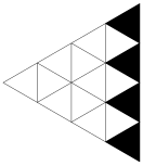
$\xrightarrow{\displaystyle\text{\ forced tiling\ }}$

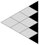
Figure 3: Example of a forced tiling of a triangular region emanating from mandatory points (represented by the smaller black triangles). Since there is only one way to tile such a region, removing it will not influence the final count.

Next, we apply a very important rule: we say that we only want to count cyclically symmetric tilings of this holey hexagon. This ensures that we only count tilings that match the tilings from one of the triplicated lozenges. We can make a few observations by imposing this new condition. First, a full tile is allowed at the optional point connection (and it will appear depending on the tiling that we are considering). Second, the mandatory points will not have a counterpart on the other side of the border and this provides a natural perimeter to prevent the counting of tilings that do not fit with our problem. Third, the space between the vertices of the central triangular hole and the mandatory points exists if $t>0$ (or $s>0$ in the analogous case). A full tile will never cross the border here. Figure 4 illustrates a region to be tiled and depicts a tiling with this rule applied.

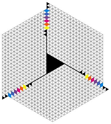
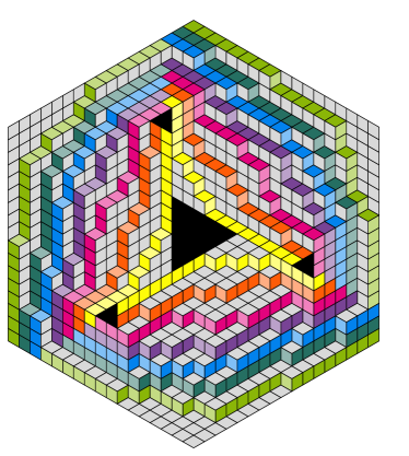
Figure 4: The region on the left corresponds to the parameters $(s,t,n,\mu)=(5,7,8,8).$ On the right, we illustrate one cyclically symmetric tiling of this region. In this example, the optional starting points $1,2,3,4,6$ (corresponding to the colors yellow, orange, red, purple, and light blue) are “activated” while from number $5$ no path is emerging.

We summarize how we do this region construction more concretely in terms of our parameters under the given assumptions (with periodic commentary in brackets to indicate the analogous case), and provide some examples in Figure 5. Set $\Delta=n-(s-t)$ to be the number of Kronecker deltas present in the matrix. We begin with a lozenge of size $n\times(\mu+s+n-2)$ with the longer edge on the bottom and shorter edge on the left (this is reversed in the analogous case, as in Figure 4 and the right side of LABEL:fig:hexfortriangle). Then, we divide the bottom edge into five parts of the following lengths:

$$\underbrace{\mu-2}_{\text{hole}}\quad+\underbrace{\vphantom{\mu}t}_{\text{border line}}+\underbrace{\vphantom{\mu}s-t}_{\text{no start points}}+\underbrace{\vphantom{\mu}\Delta}_{\text{optional start points}}+\underbrace{\vphantom{\mu}s-t}_{\text{mandatory start points}},$$

and divide the left edge into three parts of the following lengths:

$$\underbrace{t}_{\text{border line}}+\underbrace{s-t}_{\text{mandatory end points}}+\underbrace{\Delta}_{\text{optional end points}}.$$

Here, the start and end points refer to the start and end points of the paths we want to count and are represented by half-rhombi (i.e., triangles) rather than full tiles. These start points (ordered from left to right along the bottom edge) and end points (ordered from bottom to top along the side edge) are in one-to-one correspondence with the rows and columns of the original matrix, respectively. Their presence or absence is triggered by the set $I$ (see Figure 2).

We proceed by copying/pasting this lozenge twice (so now there are three total), and then rotating the copied lozenges by $120^{\circ}$ and $240^{\circ}$, respectively. Next, we glue them together exactly at the positions corresponding to $\Delta$. These paired points are indicated by the colored tiles. Furthermore, we apply a thickened border line of length $t$ on all edges starting from one vertex of the central triangular hole to the first triangle corresponding to the closest mandatory point. This is to prevent tiles from spilling over at these connections (there are no start/end points here). Lastly, we remove all forced tilings as described in Figure 3 (the bottom row of Figure 5 illustrates the corresponding regions after such a removal). Our sum of minors formula can now be interpreted in three different ways:

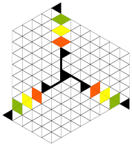
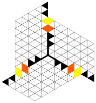
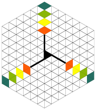
$\downarrow$	$\downarrow$	$\downarrow$	$\downarrow$

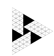
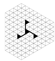
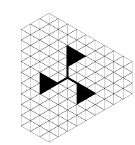
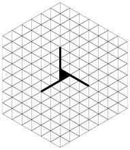
Figure 5: Selected examples of the region related to the determinant $E_{s,t}^{\mu}(n)$. From left to right $(s,t,n,\mu):(3,0,3,4),(2,1,4,3),(3,1,4,2),(2,2,4,3).$ All regions are hexagonal after the forced tiling removal, except for the left-most one, which becomes triangular. The regions will typically have four triangular holes after the forced tiling removal. Exceptions are the right-most case, which has no mandatory points, and the one to its left, where the central hole has size $0$.

• $s=t$ : $\sum_{I\subseteq\{1,\ldots,n\}}B_{I}^{I}$ counts all tuples of non-intersecting paths for all subsets of start points (and the same subsets of end points), all tilings of a lozenge-shaped region with the appearance of optional points controlled by the set $I$, and equivalently the number of cyclically symmetric tilings of the corresponding hexagonal-shaped region (which may have a central triangular hole and some border lines as described in the above construction).

• $s>t$ : $\sum_{I\subseteq\{1,\ldots,n-(s-t)\}}B_{I+s-t}^{I}$ counts all tuples of non-intersecting paths for all subsets that must contain the last $s-t$ start points and the first $s-t$ end points, all tilings of a lozenge-shaped region with the appearance of optional points controlled by the set $I$, and equivalently the number of cyclically symmetric tilings of the corresponding hexagonal or triangular shaped region (which may have up to four central triangular holes and some border lines as described in the above construction).

• $s<t$ : Analogous to $s>t$.

Next, we think about the sign. If $s-t+1$ is even, $E^{\mu}_{s,t}(n)$ counts exactly the number of cyclically symmetric rhombus tilings of the constructed region as described above, regardless of the parity of $|I|$. This is because an even sign implies that all of the possible paths/tilings that should be counted are included in the summation.

In the case where $s-t+1$ is odd, we may want to consider which terms are being cancelled in the sum. The sign $(-1)^{(s-t+1)|I|}$ indicates that we should think more carefully about the set $I$. Recall that this set controls the number of horizontal rhombi that crosses the border connections of the lozenges, in other words, they control the number of optional points that are present or absent. One way that we can take advantage of this fact is to use the symmetry of the region to be tiled to deduce conditions on $n$ and $s$ for which we can definitely see a cancellation.

We use the example of $s>t$ where $t=0$, and refer to Figure 6 for a visual. We are now in the case where we do not have a border line. This means that the four central triangular holes force the tiling of three lozenge-shaped regions (which are indicated in gray in Figure 6). Their removal will not affect the final tiling count. Thus, we can view our tiling region to be a hexagon with only one large central triangular hole! We observe that there are three lines of symmetry of this new triangular hole (in fact, they are the lines of symmetry for the whole region, one of which is shown on the left in Figure 6).

The collection of starting points that get removed by the set $I$ trigger $n-s-|I|$ paths that start at the left edge of the green lozenge and exit it at its bottom. They then enter the yellow lozenge and continue to meander around the central hole, until they complete their cycle. The third (purple) lozenge contains the red triangle. Note that the $n-s-|I|$ tiles crossing the vertical side of the red triangle imply that exactly $|I|$ tiles will cross its lower-left boundary (an example of such behavior is shown on the right in Figure 6). The symmetry of the figure (along the dashed line) now implies that there is a one-to-one correspondence between tilings with $n-s-|I|$ crossings and tilings with $|I|$ crossings. And so, if $n-s$ is odd, we will get our cancellations in (10). This allows us to deduce the identity

$$E_{0,0}^{\mu}(2m-1)=0$$

combinatorially (using $n=2m-1$ and $s=0$). Since the exact same reasoning [KoutschanThanatipanonda19] was used to deduce that $D_{1,0}^{\mu}(2m)=0$, we can conjecture a more general identity to relate the $D$ and $E$ determinants and then use a combinatorial argument to resolve it.

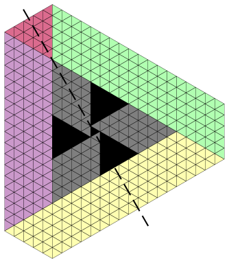
Figure 6: On the left, we present the hexagonal region associated to $(s,t,n,\mu)=(4,0,9,3)$. Observe that $s-t+1=3$ and $n-s=5$ are both odd. Forced tilings are shaded in gray, and the regions to be tiled are in different (lighter) colors. On the right is a zoomed in version of the red triangle, with an example tiling triggered by the set $I$ where $|I|=3$ tiles are removed. This gives us paths that are indicated by the $n-s-|I|=2$ dark tiles along its vertical edge that must end on the other side. Note that this forces $|I|=3$ dark tiles to appear on the other side.

Lemma 8.

For an indeterminate $\mu$ and $n,s\in\mathbbm{Z}$ such that $n\geqslant s\geqslant 1$ and $n>1$,

$$E_{s,0}^{\mu}(n) =D_{s-1,0}^{\mu+3}(n-1),$$

$$D_{s,0}^{\mu}(n) =E_{s-1,0}^{\mu+3}(n-1).$$

Proof.

If $n$ and $s$ are arbitrarily fixed integers such that $n\geqslant s\geqslant 1$ and $n>1$, then all determinants in the statement of the lemma are polynomials in $\mu$ (because the matrix entries themselves are polynomials in $\mu$). For integral $\mu$ satisfying the condition $\mu+s\geqslant 2$, we can invoke the combinatorial interpretation described above. For each identity, we will show that the determinants (i.e., the polynomials) agree for infinitely many $\mu$, and this will allow us to make our conclusion.

The first identity (the second identity is deduced analogously) can be seen using the sum of minors formula, where we simply need to observe that the number of Kronecker deltas and the sign remain the same if $n$ and $s$ are both shifted by 1. Thus, the sign patterns associated to the determinants in the sum are the same (which means we do not need to separate odd/even cases). So it is enough to show that the smaller determinants in the summands all count the same objects for all integral $\mu\geqslant 2-s$. The construction as described above is applicable for this purpose since the construction itself does not take into account these weights, so we can use it for both $\mathcal{D}_{s-1,0}^{\mu+3}(n-1)$ and $\mathcal{E}_{s,0}^{\mu}(n)$ and show that the resulting regions that need to be tiled are the same.

The lozenge associated to $\mathcal{D}_{s-1,0}^{\mu+3}(n-1)$ actually has a longer bottom edge (+1) and shorter left edge ($-1$). So as a single lozenge, it is difficult to argue that we can get the same tilings. But viewed as a holey hexagon, it is much easier! First, the removal of the triangular region (of side length $s$) associated to the mandatory points on the longer edge forces the hexagon to be the same size as the one associated to $\mathcal{E}_{s,0}^{\mu}(n)$. So now, we just need to argue about the four triangular holes in the middle, which have different sizes! But we are in the case $t=0$, and the magic is that there is only one way to tile the three lozenge-shaped regions that are forced by the four triangular holes. The removal of the additional forced tiling creates the larger triangular hole. For $\mathcal{E}_{s,0}^{\mu}(n)$, this larger triangle has length $\mu-2+3s$ and for $\mathcal{D}_{s-1,0}^{\mu+3}(n-1)$, this larger triangle has the same length: $(\mu+3)-2+3(s-1)=\mu-2+3s$ (see Figure 7). If $n=s$, then there is only one big triangle in both cases, so this is trivially equal. We also remark that an algebraic proof of this lemma can be realized by applying certain row and column operations to the matrices. For this, we refer the reader to the discussion in the proof of Lemma 10.

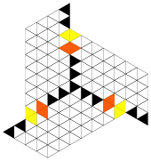
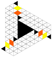
$\downarrow$	$\downarrow$

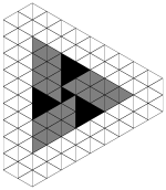
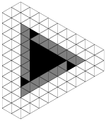
Figure 7: Pinwheel and hexagon figures for $(s,t,n,\mu)=(2,0,4,3)$ in Lemma 8. The left column is associated to $\mathcal{E}_{s,0}^{\mu}(n)$ and the right column is associated to $\mathcal{D}_{s-1,0}^{\mu+3}(n-1)$. Note that the region to be tiled is the same in both cases (after removing all regions of forced tilings).

∎

Corollary 9.

For an indeterminate $\mu$ and $m,r\in\mathbbm{Z}$ such that $m>r\geqslant 0$, denote

$$P_{m,r}:=\prod_{i=1}^{m-r-1}\frac{\bigl{(}\mu+2i+6r\bigr{)}_{i}^{2}\,\bigl{(}\frac{\mu}{2}+2i+3r+1\bigr{)}_{i}^{2}}{\bigl{(}i+1\bigr{)}_{i}^{2}\,\bigl{(}\frac{\mu}{2}+i+3r\bigr{)}_{i}^{2}}.$$

Then $E_{2r,0}^{\mu}({2m-1})=0$ and

$$E_{2r,0}^{\mu}({2m}) =\frac{(-1)^{m-r}\,\bigl{(}\frac{\mu}{2}+3r-\frac{1}{2}\bigr{)}_{m-r}}{\bigl{(}\frac{1}{2}\bigr{)}_{m-r}}\cdot P_{m,r},$$

$$E_{2r+1,0}^{\mu}({2m-1}) =\frac{\bigl{(}m-r\bigr{)}_{m-r-1}}{\bigl{(}\frac{\mu}{2}+2m+r-1\bigr{)}_{m-r-1}}\cdot P_{m,r},$$

$$E_{2r+1,0}^{\mu}({2m}) =\frac{2\,\bigl{(}\mu+2m+4r+1\bigr{)}_{m-r-1}}{\bigl{(}\frac{\mu}{2}+m+2r+1\bigr{)}_{m-r-1}}\cdot P_{m,r}.$$

Proof.

These formulas follow directly from [KoutschanThanatipanonda19, Theorems 18 and 19] by using Lemma 8. ∎

4 Closed Forms for $\bm{E_{2r-1,1}^{\mu}({2m-1})}$ and $\bm{D_{2r,1}^{\mu}({2m})}$

The main goal of this section is to derive closed forms for the determinants $E_{2r-1,1}^{\mu}(2m-1)$ and $D_{2r,1}^{\mu}(2m)$. This allows us to resolve two conjectures [Krattenthaler05, Conjecture 37] and [KoutschanThanatipanonda19, Conjecture 20]. We note that this is the first time that we are able to prove non-trivial results for whole families of determinants (with $s$ or $t$ containing a parameter). The roadmap for how we do this can be seen in Figure 1 in the color blue and summarized as follows:

• The key result is Lemma 10, where we establish the ratios between families $E_{2r-1,1}^{\mu}(2m-1)$ and $D_{2r,1}^{\mu}(2m)$.

• This connection between the determinants along with the base case $E_{1,1}^{\mu}(2m-1)$, whose closed form was already derived in [KoutschanThanatipanonda13, Theorem 2] and presented in LABEL:prop:E11, allows us to realize the first main result, a closed form for $E_{2r-1,1}^{\mu}(2m-1)$ in

In Lemma 10, we first process the matrix by multiplying with two elementary matrices $\mathcal{L}_{n}$ and $\mathcal{R}_{n}$, which we define in (13). Then we apply a variant of the holonomic ansatz as described in Section 2.3, to set up the problem so that the computer can be used to prove our result with the machinery described in Section 2.4. The introduction of the new parameter $r$ causes more difficulties in the calculation than usual. We discuss these difficulties in the proof below.

Lemma 10.

Let $\mu$ be an indeterminate, and $m,r\in\mathbbm{Z}$. If $m\geqslant r\geqslant 1$, then

$$\frac{D_{2r,1}^{\mu}({2m})}{E_{2r-1,1}^{\mu+3}({2m-1})} =\frac{(m+r-1)(\mu-1)(\mu+2m+1)(\mu+2r)}{2m(2r-1)(\mu+2)(\mu+2m+2r-1)},$$ (11)

$$\frac{E_{2r+1,1}^{\mu}({2m+1})}{D_{2r,1}^{\mu+3}({2m})} =\frac{(m+r)(\mu-1)(\mu+2m+2)(\mu+2r+1)}{2r(2m+1)(\mu+2)(\mu+2m+2r+1)}.$$ (12)

Proof.

We first observe that the two identities can be presented in a uniform way:

$$\frac{A_{s,1}^{\mu}(n)}{B_{s-1,1}^{\mu+3}({n-1})}=\frac{(n+s-2)(\mu-1)(\mu+n+1)(\mu+s)}{2n(s-1)(\mu+2)(\mu+n+s-1)}=:R_{s,1}^{\mu}(n),$$

where $(A,B,s,n)=(D,E,2r,2m)$ or $(A,B,s,n)=(E,D,2r+1,2m+1)$. Since we are dealing with ratios of determinants, we first make sure that a division by zero will not occur. To do this, we employ an inductive argument with respect to $n$, in order to show that all determinants that will be used in the proof are nonzero: for the induction base, we note that $E_{1,1}^{\mu}({n})\neq 0$ by [KoutschanThanatipanonda13, Theorem 2] (see also LABEL:prop:E11), the induction hypothesis is $B_{s-1,1}^{\mu+3}({n-1})\neq 0$, and the induction step is completed once the identities (11) and (12) are established (note that both ratios on the right-hand sides are never identically zero under the stated assumption $m\geqslant r\geqslant 1$). In each step of the induction, the roles of $D$ and $E$ are interchanged, which is reflected by the zigzag arrangement of the blue connections in Figure 1.

Next, we manipulate the matrix $\mathcal{A}_{s,1}^{\mu}(n)$ so that its determinantal value remains unaffected:

$$\mathcal{L}_{n}\cdot\mathcal{A}_{s,1}^{\mu}(n)\cdot\mathcal{R}_{n}=:\tilde{\mathcal{A}}_{s,1}^{\mu}(n),$$

where $\mathcal{L}_{n},\mathcal{R}_{n}\in\mathbbm{R}^{n\times n}$ are such that

$$\mathcal{L}_{n}:=\begin{pmatrix}1&0&0&0&\cdots\\ -1&1&0&0&\cdots\\ 0&-1&1&0&\cdots\\ 0&0&-1&1&\cdots\\ \vdots&\vdots&\vdots&\vdots&\ddots\end{pmatrix}\qquad\mbox{and}\qquad\mathcal{R}_{n}:=\begin{pmatrix}1&1&1&1&\cdots\\ 0&1&1&1&\cdots\\ 0&0&1&1&\cdots\\ 0&0&0&1&\cdots\\ \vdots&\vdots&\vdots&\vdots&\ddots\end{pmatrix}.$$ (13)

The matrices $\mathcal{L}_{n}$ and $\mathcal{R}_{n}$ perform elementary row resp. column operations that exploit the elementary property (2) of the binomial coefficient. We also note that the determinants of both matrices are $1$.

Using Lemma 2, the resulting matrix is

$$\tilde{\mathcal{A}}_{s,1}^{\mu}(n)=\left(\begin{array}[]{c:c}\binom{\mu+s-1}{1}&\binom{\mu+j+s-1}{j}-1\pm\sum\limits_{k=1}^{j}\delta_{s,k}\\ &\scriptstyle(2\;\leqslant\;j\;\leqslant\;n)\\ \hdashline&\\[-12.0pt] 1&\binom{\mu+i+j+s-3}{j-1}\mp\delta_{s,j-i+2}\\ \scriptstyle(2\;\leqslant\;i\;\leqslant\;n)&\scriptstyle(2\;\leqslant\;i,j\;\leqslant\;n)\end{array}\right),$$

where $\pm$ is $+$ if $A=D$ and $-$ if $A=E$ (and $\mp$ is $-$ if $A=D$ and $+$ if $A=E$). We observe that the bottom right $(n-1)\times(n-1)$ submatrix is $\mathcal{B}_{s-1,1}^{\mu+3}(n-1)$. In other words, the “other” family (i.e., a matrix with the Kronecker delta of opposite sign modulo shifts in $\mu$ and $s$) appears. We can now adapt the holonomic ansatz (see Section 2.3) to our problem. To compute the determinant of $\tilde{\mathcal{A}}_{s,1}^{\mu}(n)$, we choose to expand about the first row (rather than the last row) to get

$$\tilde{A}_{s,1}^{\mu}(n)=\tilde{a}_{1,1}\cdot\text{Cof}_{1,1}(n-1)+\cdots+\tilde{a}_{1,n}\cdot\text{Cof}_{1,n}(n-1),$$

where $\tilde{a}_{i,j}$ is the $(i,j)$-entry of $\tilde{\mathcal{A}}_{s,1}^{\mu}(n)$, and $\text{Cof}_{1,j}(n-1)$ is the corresponding cofactor. Then $B_{s-1,1}^{\mu+3}({n-1})=\text{Cof}_{1,1}(n-1)$, which by the induction hypothesis is nonzero. Hence, we can define

$$c_{n,j}:=\frac{\text{Cof}_{1,j}(n-1)}{\text{Cof}_{1,1}(n-1)},$$ (14)

and our formulas (11) and (12) will be confirmed by showing that for all $n\geqslant s$:

$$\sum\limits_{j=1}^{n}\tilde{a}_{1,j}\cdot c_{n,j}=R_{s,1}^{\mu}(n).$$ (15)

Unfortunately, we cannot get a closed form for the $c_{n,j}$’s for symbolic $n$ and $j$, in order to prove (15). Instead, we will construct an implicit description of the bivariate sequence $c_{n,j}$ in terms of recurrences, and then employ the holonomic framework to prove (15).

We can compute many values $c_{n,j}$ explicitly for fixed integers $n$ and $j$, and then proceed to “guess” (i.e., interpolate) recurrences which the $c_{n,j}$’s satisfy, using an appropriate guessing program (for our purposes, we use [Kauers09]). However, since these recurrences were obtained from a finite amount of data, we need to substantiate their universal validity, that is for all $n$ and $j$. This is done by observing that the following identities uniquely characterize the $c_{n,j}$’s

$$\begin{cases}\;c_{n,1}=1,&n\geqslant 1,\\[4.30554pt] \;\displaystyle\sum_{j=1}^{n}\tilde{a}_{i,j}\cdot c_{n,j}=0,&2\leqslant i\leqslant n,\end{cases}$$ (16)

because by the induction hypothesis, the matrix $\mathcal{B}_{s-1,1}^{\mu+3}(n-1)=(\tilde{a}_{i,j})_{2\leqslant i,j\leqslant n}$ has full rank. Hence, if we confirm that a suitable solution of the guessed recurrences satisfies (16), then we can conclude that it completely agrees with $c_{n,j}$. Of course, we will employ the holonomic framework for this task. Less importantly, we remark that the data generation for the guessing is achieved more efficiently using the system (16) rather than using the definition (14) in terms of minors.

To prove (11), we use $(A,B,s,n)=(D,E,2r,2m)$ and show that the $c_{2m,j}$ satisfy the identities corresponding to (16) and (15) for all $m\geqslant r$:

$$c_{2m,1} =1,$$

$$\sum_{j=1}^{2m}\binom{\mu+i+j+2r-3}{j-1}\cdot c_{2m,j}-c_{2m,i+2r-2} =0,\qquad(2\leqslant i\leqslant 2m),$$

$$\sum_{j=1}^{2m}\binom{\mu+j+2r-1}{j}\cdot c_{2m,j}-\sum_{j=1}^{2r-1}c_{2m,j} =R_{2r,1}^{\mu}(2m).$$

To prove (12), we use $(A,B,s,n)=(E,D,2r+1,2m+1)$ and show that the $c_{2m+1,j}$ satisfy the identities corresponding to (16) and (15) for all $m\geqslant r$:

$$c_{2m+1,1} =1,$$

$$\sum_{j=1}^{2m+1}\binom{\mu+i+j+2r-2}{j-1}\cdot c_{2m+1,j}+c_{2m+1,i+2r-1} =0,\qquad(2\leqslant i\leqslant 2m+1),$$

$$\sum_{j=1}^{2m+1}\binom{\mu+j+2r}{j}\cdot c_{2m+1,j}-\sum_{j=1}^{2r}c_{2m+1,j}-\sum_{j=2r+1}^{2m+1}2\cdot c_{2m+1,j} =R_{2r+1,1}^{\mu}(2m+1).$$

At this point, the computer steps in to do some of the legwork for us, and we briefly talk here about the computation part of the proof (see Section 2.4 and [EM2]). From the guessing step, we already have the generators for a left annihilating ideal of the $c$’s and we can see that all of the other constituents in these identities are binomial coefficients or rational functions in the parameters, which have the nice property of being holonomic. We also note that the summations in the identities have “natural boundaries” in that the summands evaluate to zero beyond the summation bounds. This means that when we apply creative telescoping and closure properties for holonomic functions to our objects (see [Zeilberger90, Koutschan09]), we expect to be able to deduce an annihilating ideal for the left-hand sides without further adjustments. We can simplify things by moving terms that are not a summation to the right-hand side and computing an annihilating ideal for them separately (this is to avoid a possible slowdown from the need to apply additional closure properties). The last step is to confirm that either the annihilating ideals on both sides are equal, or one is a subideal of the other, along with comparing a sufficient number of initial values.

In theory, the procedure described above is expected to be relatively uncomplicated. Unfortunately, in practice it turned out to be a bit painful and we take a couple of paragraphs to highlight two difficulties that were encountered during the computation. All of the details can be found in the online supplementary material [EM2].

1. Creative telescoping on the summation in the second identity of (16) did not finish (we left it running to see if it would, but in the third month a water leak in the building destroyed the node the computations were on). This meant that we needed a better way to speed up the process. This was achieved by interpolating/guessing telescoping relations for the generators of the annihilating ideals for the sum. We confirmed that our guesses are correct by showing that they lie in the annihilating ideal of the summands. We then extracted annihilators for the sum from these relations (i.e., the telescopers). A second trick to speed up this computation was not to construct the full Gröbner basis this way, but only a few generators (concretely: two out of three), and then run Buchberger’s algorithm to obtain the remaining ones.

   The timing to confirm the second identity of (16) was roughly 8 hours in each of the two cases, and most of the time was taken to generate the data for interpolating the telescoping relations.

2. Applying creative telescoping on the summations in the third identity corresponding to (15) resulted in the appearance of singularities in the certificates within the summation range. This meant that we were unable to certify that our telescopers were the correct annihilators of the sums. There is a way to fix this by hand (see [KoutschanWong21] for examples and an easy-to-digest description) which involves removing the places where the singularity occurs and collecting inhomogeneous parts to compensate for the removal. Using this strategy, the final annihilator for each sum would consist of a “left multiplication” of the annihilator of these inhomogeneous parts to the original telescoper. When we applied this strategy, we encountered a problem in our computation because the annihilator of one of the inhomogeneous parts was unable to finish computing and this required another human interaction to complete the process. In particular, the difficulty occurred in a substitution step. So instead of applying the substitution command directly (which is an implementation of the corresponding closure property), we performed the substitution by hand on the coefficients of the computed annihilator and then searched for the final annihilator that had the support that we expected after substituting.

   The timing to achieve a “grand” recurrence for the left-hand sides of the identities (11) and (12) corresponding to (15) was roughly 30 hours each, with most of the time taken to deal with the inhomogeneous parts. In both cases, the recurrence is of order $7$ in $m$ with an approximate byte count of 66,000,000. The degrees of the polynomial coefficients in the parameters $m,r,\mu$ are $47$, $37$, and $38$, respectively. ∎

We now introduce a technical lemma that will enable us to convert the formula for $E_{1,1}^{\mu}({2m-1})$ given in [KoutschanThanatipanonda13, Theorem 2] into a nicer form in LABEL:prop:E11.

Lemma 11.

Let $\mu$ be an indeterminate and $m\in\mathbbm{Z}$ with $m\geqslant 1$. Then

$$2^{(m-1)(m-2)/2}\cdot\prod_{i=1}^{\left\lfloor m/2\right\rfloor}\bigl{(}\tfrac{\mu}{2}+3i-\tfrac{1}{2}\bigr{)}_{\!m-2i}\,\bigl{(}\tfrac{\mu}{2}+2m-i\bigr{)}_{\!m-2i+1}=\prod_{i=1}^{m-1}\frac{\bigl{(}\mu+2i+1\bigr{)}_{i-1}\,\bigl{(}\frac{\mu}{2}+2i+1\bigr{)}_{i}}{\bigl{(}\frac{\mu}{2}+i+1\bigr{)}_{i-1}}.$$

Proof.

The proof goes by induction with respect to $m$. Let $L_{m}$ and $R_{m}$ denote the left-hand (resp. right-hand) side of the statement. For $m=1$, we get $L_{1}=1=R_{1}$. For all integers $m\geqslant 1$, we have the relations

$$\frac{R_{m+1}}{R_{m}} =\frac{\bigl{(}\mu+2m+1\bigr{)}_{m-1}\,\bigl{(}\frac{\mu}{2}+2m+1\bigr{)}_{m}}{\bigl{(}\frac{\mu}{2}+m+1\bigr{)}_{m-1}},$$

$$\frac{L_{m+1}}{L_{m}} =\begin{cases}\displaystyle\frac{2^{m-1}\left(\frac{\mu}{2}+m+\frac{1}{2}\right)_{\frac{m}{2}}\left(\frac{\mu}{2}+\frac{3m}{2}+1\right)_{\frac{3m}{2}}}{\left(\frac{\mu}{2}+\frac{3m}{2}\right)_{\frac{m}{2}}\left(\frac{\mu}{2}+\frac{3m}{2}+1\right)_{\frac{m}{2}}}&\mbox{if $m$ is even,}\\[17.22217pt] \displaystyle\frac{2^{m-1}\left(\frac{\mu}{2}+m+\frac{1}{2}\right)_{\frac{m-1}{2}}\left(\frac{\mu}{2}+\frac{3m}{2}+\frac{3}{2}\right)_{\frac{3m-1}{2}}}{\left(\frac{\mu}{2}+\frac{3m}{2}+\frac{1}{2}\right)_{\frac{m-1}{2}}\left(\frac{\mu}{2}+\frac{3m}{2}+\frac{3}{2}\right)_{\frac{m-1}{2}}}&\mbox{if $m$ is odd,}\end{cases}$$

where $L_{m+1}/L_{m}$ comes from rearranging the Pochhammers so that (P8) can be applied. Then, a strategic application of the Pochhammer properties (P5), (P4), (P3) to $L_{m+1}/L_{m}$ for both cases enables us to conclude that $L_{m+1}/L_{m}=R_{m+1}/R_{m}$. Thus, $L_{m}=R_{m}$ for all $m\geqslant 1$. ∎

LABEL:prop:E11 presents a closed form for $E_{1,1}^{\mu}(2m-1)$, which will be used as a base case for our main results (

Theorem 10

Krat37nice and