Predictive feedback boundary control of semilinear and quasilinear $2\times 2$ hyperbolic PDE-ODE systems

Abstract

We present a control design for semilinear and quasilinear $2\times 2$ hyperbolic partial differential equations with the control input at one boundary and a nonlinear ordinary differential equation coupled to the other. The controller can be designed to asymptotically stabilize the system at an equilibrium or relative to a reference signal. Two related but different controllers for semilinear and general quasilinear systems are presented and the additional challenges in quasilinear systems are discussed. Moreover, we present an observer that estimates the distributed PDE state and the unmeasured ODE state from measurements at the actuated boundary only, which can be used to also solve the output feedback control problem.

AND

, ,

1 Introduction

In this paper, we consider systems consisting of a 1-d hyperbolic partial differential equation (PDE) coupled with an ordinary differential equation (ODE) at the uncontrolled boundary, as given by

$$w_{t}(x,t) =\Lambda(x,w(x,t))\,w_{x}(x,t)+F(x,w(x,t)),$$ (1)

$$\dot{X}(t) =f^{0}(X(t),v(0,t),t),$$ (2)

$$u(0,t) =g^{0}(X(t),v(0,t),t),$$ (3)

$$v(1,t) =U(t),$$ (4)

$$w(\cdot,0) =w_{0}=\left(\begin{matrix}u_{0}&v_{0}\end{matrix}\right)^{T},$$ (5)

$$X(0) =X_{0}.$$ (6)

Here $w(x,t)=\left(\begin{matrix}u(x,t)&v(x,t)\end{matrix}\right)^{T}$, $X(t)\in\mathbb{R}^{n}$, subscripts denote partial derivatives, $x\in[0,1]$, $t\geq 0$, $w_{0}$ and $X_{0}$ are initial conditions, and $U$ is the control input. The nonlinear functions $\Lambda$ and $F$, which model the propagation speeds and source terms, respectively, have the structure

$$\Lambda(x,z) =\left(\begin{matrix}-\lambda^{u}(x,z)&0\\ 0&\lambda^{v}(x,z)\end{matrix}\right), \lambda^{u},\,\lambda^{v} >0,$$ (7)

$$F(x,z) =\left(\begin{matrix}f^{u}(x,z)&f^{v}(x,z)\end{matrix}\right)^{T}.$$ (8)

The nonlinear functions $f^{0}$ and $g^{0}$ define the coupling to the ODE at the uncontrolled boundary. More precise assumptions on the system data are given in the subsequent sections.

The system is called semilinear in the special case where $\Lambda$ is independent of the state $w(x,t)$, whereas a quasilinear system is the general case when $\Lambda$ is a function of the state $w(x,t)$. The difference between semilinear and quasilinear systems is significant. In particular, the characteristic lines of quasilinear systems depend on the state and the control input. If characteristic lines “collide”, the solution ceases to exist due to blow-up of the gradient of that state, even if the state itself remains bounded [2]. Therefore, the control inputs need to be designed not only to regulate the state, but also to prevent a collision of characteristic lines. By contrast, the characteristic lines of semilinear (including linear) systems are known a priori and they do not collide, which simplifies the control design. The dependence of $\Lambda$ on the state also has implication on the state space. For semilinear systems, so called broad solutions [2, Chapter 3] can be defined over $L^{\infty}$. That is, the solutions can be discontinuous and the control inputs can be chosen freely in $L^{\infty}$. In quasilinear systems, at least Lipschitz-continuity of the state is required in order to define broad solutions. As a consequence, the control inputs must be compatible with the current state at all times, and there is a limit on how fast the system can be steered to the desired state.

Hyperbolic systems similar to (1) have received significant attention. They model several 1-d transport phenomena such as gas or fluid flow through pipelines, open-channel flow, traffic flow and electrical transmission lines [1]. Control design approaches for these systems include dissipative boundary conditions [8] and control Lyapunov functions [3]. However, the use of such static boundary feedback works only if the source terms are small [1]. An alternative approach for linear systems that steers the system more actively to the desired state is backstepping, which now exists for a variety of system classes, see e.g. [10, 22, 4]. Motivated by an application to mechanical vibrations in drill strings [5], a backstepping controller for PDE-ODE systems similar to those considered here is developed in [6], although only for linear systems. A different approach has been pursued in [16, 20] for semilinear systems and in [19, 21] for quasilinear systems, which achieves performance equivalent to that of backstepping controllers, but for nonlinear systems. In [21], robustness to parameter uncertainty and measurement and actuation errors is also investigated.

The contributions of this paper extend [21] to hyperbolic systems that are coupled with a nonlinear ODE at the uncontrolled boundary, as given by (1)-(6). Moreover, we present an observer that estimates the distributed PDE state $w$ and the ODE state $X$ from boundary measurements of $u$ at the actuated boundary only.

The paper is organized as follows. First, the state feedback control design for semilinear systems is presented in Section 2. The control design for quasilinear systems is given in Section 3. The observer is presented in Section 4. In Section 5, a simulation study is performed to demonstrate the effectiveness of the proposed controller. Section 6 contains some concluding remarks.

2 Semilinear systems

The control design proposed here for semilinear systems builds on ideas first presented in [16]. The approach is based on the following two observations:

• Due to the hyperbolic nature of Equation (1), the effect of the control input entering in boundary condition (4) propagates through the domain with finite speed $\lambda^{v}$. Therefore, the state $w$ in the interior of the domain and the state $X$ of the ODE (2), are only affected after a certain amount of time has passed.

• The system is easier to control by treating $v(0,\cdot)$, the value of $v$ at the uncontrolled boundary, as a “virtual” control input $U^{*}$. This is because $v(0,\cdot)$ enters both the boundary condition for $u$, as given in (3), and in the ODE (2), whereas the coupling between $U$ and the states $u$ and $X$ is more indirect and affected by the delay. In a second step, the actual inputs $U$ can be constructed such that $v(0,\cdot)$ becomes equal to $U^{*}$.

For semilinear systems, we present a continuous-time state feedback control law. At each time $t$ the controller maps the state $(w(\cdot,t),\,X(t))$ into the control input $U(t)$. This state feedback controller can be combined with the observer from Section 4 to obtain an output feedback controller.

2.1 Assumptions

For semilinear systems considered in this section, we make the following assumptions.

Assumption 1.

The speeds in $\Lambda$ are assumed to be independent of the state $w$. The speeds are bounded from below by

$$\sup_{x\in[0,1]}\min\{(\lambda^{u}(x))^{-1},\,(\lambda^{v}(x))^{-1}\}\leq l_{\Lambda^{-1}}.$$ (9)

The nonlinear functions $F$, $f^{0}$, $g^{0}$ are globally Lipschitz-continuous in the state arguments, i.e.,

$$\operatorname*{ess\,sup}_{x\in[0,1],w\in\mathbb{R}^{2}}\|\partial_{w}F(x,w)\|_{\infty} =l_{F},$$ (10)

$$\operatorname*{ess\,sup}_{X\in\mathbb{R}^{n},v\in\mathbb{R},t\geq 0}|\partial_{X}f^{0}(X,v,t)| =l_{f^{0}_{X}},$$ (11)

$$\operatorname*{ess\,sup}_{X\in\mathbb{R}^{n},v\in\mathbb{R},t\geq 0}|\partial_{v}f^{0}(X,v,t)| =l_{f^{0}_{v}},$$ (12)

$$\operatorname*{ess\,sup}_{X\in\mathbb{R}^{n},v\in\mathbb{R},t\geq 0}|\partial_{X}g^{0}(X,v,t)| =l_{g^{0}_{X}},$$ (13)

$$\operatorname*{ess\,sup}_{X\in\mathbb{R}^{n},v\in\mathbb{R},t\geq 0}|\partial_{v}g^{0}(X,v,t)| =l_{g^{0}_{v}},$$ (14)

where $\partial$ denotes partial derivatives and $l_{F}$ through $l_{g^{0}_{v}}$ are the finite Lipschitz constants. We assume further that

$$F(x,0) =0 x\in[0,1],$$ for all (15)

$$f^{0}(0,0,t) =g^{0}(0,0,t)=0 t\geq 0,$$ for all (16)

which ensures that the origin is an equilibrium. Finally, assume there exists a controller $K(X(t),t)$ satisfying

$$\operatorname*{ess\,sup}_{X\in\mathbb{R}^{n},t\geq 0}|\partial_{X}K(X,t)| =l_{K},$$ (17)

$$K(0,t) =0 t\geq 0,$$ for all (18)

such that the closed-loop system

$$\dot{X}(t)=f^{0}(X(t),K(X(t),t),t)$$ (19)

has a globally asymptotically stable equilibrium at the origin.

2.2 Characteristic lines and determinate sets

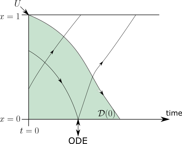
Figure 1: Characteristic lines of system (1)-(6), with the input $U$ entering at $x=1$ and the coupling with the ODE at $x=0$. The determinate set $\mathcal{D}(0)$ is shaded in green.

The characteristic lines of the system are sketched in Figure 1. We parametrize the characteristic lines of (1) via

$$\tau^{u}(t;x) =t+\int_{0}^{x}\frac{1}{\lambda^{u}(\xi,w(\xi,\tau^{u}(t;\xi))}d\xi,$$ (20)

$$\tau^{v}(t;x) =t+\int_{x}^{1}\frac{1}{\lambda^{v}(\xi,w(\xi,\tau^{v}(t;\xi))}d\xi,$$ (21)

where $\tau^{u}$ and $\tau^{v}$ are the times at which the characteristic lines that start at time $t$ and the spatial boundary $x=0$ and $x=1$, respectively, reach the location $x\in[0,1]$. The corresponding closed and half-open determinate sets are defined as

$$\mathcal{D}(t) =\left\{(x,s):\,x\in[0,1],\,s\in[t,\tau^{v}(t;x)]\right\},$$ (22)

$$\mathcal{D}^{\prime}(t) =\left\{(x,s):\,x\in[0,1],\,s\in[t,\tau^{v}(t;x))\right\}.$$ (23)

The state dependences of $\lambda^{u}$ and $\lambda^{v}$ in (20)-(21) are included so that the same definitions can be re-used in Section 3. The following lemma formalizes the above remark that the solution is independent of the control input for a certain amount of time.

Lemma 2.

Under Assumption 1, the Cauchy problem consisting of (1)-(3) with initial conditions (5)-(6), i.e., without boundary condition (4), has a unique bounded solution $u(x,t)$ for $(x,t)\in\mathcal{D}(0)$, $v(x,t)$ for $(x,t)\in\mathcal{D}^{\prime}(0)$ and $X(t)$ for $t\in[0,\tau^{v}(0;0)]$, that continuously depends on $(w_{0},X_{0})$. That is, the solution on these sets is independent of the control input $U(t)$ for $t\geq 0$.

The proof is similar to the proof of the first part of Theorem 2 in [16]. The difference is that here we have an ODE at the uncontrolled boundary compared to a static boundary condition in [16], which does not affect the determinate sets themselves. See also [12, 11, 2] for a more general discussion of determinate sets (sometimes also called domains of determinacy). The solution of $u(x,t)$ for $(x,t)\in\mathcal{D}(0)$ in Lemma 2 includes the state on the characteristic line $u(\cdot;\tau^{v}(0;\cdot))$. After shifting time, this implies that the future states $u(\cdot,\tau^{v}(t;\cdot))$ and $X(\tau^{v}(t;0))$ are predictable based on the state $w(\cdot,t)$ alone, independently of the input $U(t)$.

As is usual for hyperbolic PDEs, the state satisfies an ODE along the characteristic lines:

Lemma 3.

For given $t$, the state on the characteristic lines $(x,\tau^{v}(t;x))$, $x\in[0,1]$, satisfies

$$\frac{d}{dx}v(x,\tau^{v}(t;x)) =-\frac{f^{v}(x,(u,v)(x,\tau^{v}(t;x)))}{\lambda^{v}(x)},$$ (24)

$$v(x,\tau^{v}(t;1)) =U(t).$$ (25)

See [16, Theorem 2]. Importantly, Equation (24) can be solved in either $x$-direction. This will be exploited in the following subsection, where the desired boundary value for $v$ at $x=0$ is designed as a virtual input, and a corresponding actual actual input $U(t)$ is constructed.

2.3 Sufficient condition for global asymptotic stability

In order to see that system (1)-(6) is in fact easier to control via the boundary value of $v(0,\cdot)$, it is insightful to solve (1) for $w_{x}$, swapping the roles of $t$ and $x$ and introducing the new input $U^{*}(t)$. This gives the system

$$w_{x}(x,t) =\left(\Lambda(x,w(x,t))\right)^{-1}\left(w_{t}(x,t)-F(x,w(x,t))\right),$$ (26)

$$\dot{X}(t) =f^{0}(X(t),U^{*}(t),t),$$ (27)

$$u(0,t) =g^{0}(X(t),U^{*}(t),t),$$ (28)

$$v(0,t) =U^{*}(t),$$ (29)

$$w(\cdot,0) =w_{0}=\left(\begin{matrix}u_{0}&v_{0}\end{matrix}\right)^{T},$$ (30)

$$X(0) =X_{0}.$$ (31)

The new input $U^{*}$ now enters at the common inflow boundary condition ($x=0$) for both distributed states $u$ and $v$, and as an input for the ODE that in turn also affects only the boundary condition for $u$ at $x=0$.

Setting $U^{*}(t)=K(X(t),t)$ solves the problem of asymptotically stabilizing system (26)-(31).

Lemma 4.

Under Assumption 1, if $U^{*}(t)=K(X(t),t)$ for all $t\geq\tau^{v}(0;0)$, then (26)-(31) has a globally asymptotically stable equilibrium at the origin.

Because of Lipschitz-continuity of the data and the fact that $\Lambda$ is independent of the state, the solution cannot blow up in finite time, i.e., the solutions exists for all $(x,t)\in[0,1]\times[0,\infty)$. Similar to [21, Theorem 6], one can show that there exists some constant $\gamma\geq 1$ such that for all $T\geq 0$,

$$\sup_{x\in[0,1],\,t\geq\tau^{u}(T;x)}\|w(x,t)\|_{\infty}\leq\gamma\,\sup_{t\geq T}\|w(0,t)\|_{\infty}.$$ (32)

For $t<\tau^{v}(0;0)$, Lemma 2 ensures that both $w(0,t)$ and $X(t)$ remain bounded and the bounds depend continuously on the initial condition.

For all $t\geq\tau^{v}(0;0)$, the choice of $U^{*}$ ensures that (19) is satisfied. Thus, $X(t)$ remains bounded, and the bound during transients can be made arbitrarily small by making the initial condition small. Lipschitz-continuity of $g^{0}$ and $K$ combined with conditions (16) and (18), imply $\|w(0,\cdot)\|_{\infty}\leq\gamma^{\prime}\|X(\cdot)\|_{\infty}$ for some $\gamma^{\prime}>0$, which implies stability of the whole system. Similarly, convergence of $X$ to the origin due to asymptotic stability of (19), implies that for all $\epsilon>0$ there exists a $T\geq 0$ such that $\|X(t)\|_{\infty}\leq\epsilon$ for all $t\geq T$. Hence $\sup_{t\geq T}\|w(0,t)\|\leq\gamma^{\prime}\epsilon$. Due to (32), this implies that $w$ convergences to the origin as well.

2.4 Control law

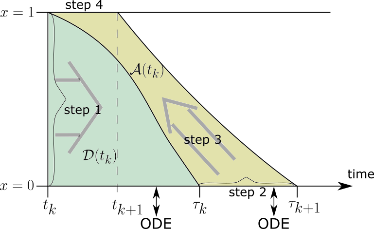
Figure 2: The steps of evaluating the controller at time $t_{k}$, at the example of the sampled-time controller for quasilinear systems: 1) predict state $w$ on determinate set $\mathcal{D}(t_{k})$ (shaded in green) and $X$ up to time $\tau_{k}$; 2) design virtual input $U^{*}$ 3) solve target system $(\bar{w}^{*},\bar{X}^{*})$ backwards over domain $\mathcal{A}(t_{k})$ (yellow); 4) set input to $U(t)=\bar{v}^{*}(1,t)$. In the semilinear case with continuous time control law, the domain $\mathcal{A}(t_{k})$ reduces to the line $(x,\tau^{v}(t_{k};x))$, $x\in[0,1]$.

With the preparations above, we are in position to synthesize the controller. The main steps for evaluating the controller are also summarized in Figure 2 and Algorithm 1 below.

Step 1: Predict state

Lemma 2 can be exploited to establish a prediction of the state on the determinate set $\mathcal{D}(t)$. To this end, denoting the prediction by $(\bar{w},\,X)$ in order to distinguish it from the actual state, we simply copy the dynamics (1)-(3) but use the current state, $(w(\cdot,t),X(t))$, as the initial condition:

$$\bar{w}_{t}(x,s) =\Lambda(x,\bar{w}(x,s))\,\bar{w}_{x}(x,s)+F(x,\bar{w}(x,s)),$$ (33)

$$\dot{\bar{X}}(s) =f^{0}(\bar{X}(s),\bar{v}(0,s),s),$$ (34)

$$\bar{u}(0,s) =g^{0}(\bar{X}(s),\bar{v}(0,s),s),$$ (35)

$$\bar{w}(\cdot,t) =w(\cdot,t)$$ (36)

$$\bar{X}(t) =X(t).$$ (37)

As stated by Lemma 2, we can solve (33)-(37) over the determinate set $\mathcal{D}(t)$ to obtain the predictions $\bar{u}(\cdot,\tau^{v}(t;\cdot))$ and $\bar{X}(\tau^{v}(t;0))$. Assuming no model uncertainty, these predictions are equal to the values that the actual state will attain. For comparison, estimates on prediction errors when there is uncertainty in parameters and measurements are given in [21], although only for static boundary conditions.

Step 2: Design virtual input $U^{*}$

By Lemma 4, the control objective of asymptotically stabilizing the system is achieved if $v(0,t)$ becomes equal to $K(X(t),t)$. The earliest time at which $U(t)$ has an effect on $v(0,\cdot)$ is given by $\tau^{v}(t;0)$, and this is also the latest time up to which we can predict $\bar{X}$. Therefore, at each time $t$ we set the future value of the virtual input to

$$U^{*}(\tau^{v}(t;0))=K(\bar{X}(\tau^{v}(t;0)),\tau^{v}(t;0)).$$ (38)

Step 3: Construct input $U(t)$

As stated in Lemma 3, $v(x,\tau^{v}(t;x))$ satisfies an ODE in $x$ that can in principle be solved in either $x$-direction. The target boundary value that $v(0,\tau^{v}(t;0))$ shall satisfy is given by (38). Thus, we can compute the required control input $U(t)$ by solving the target dynamics

$$\frac{d}{dx}\bar{v}^{*}(x,\tau^{v}(t;x)) =-\frac{f^{v}(x,(\bar{u},\bar{v}^{*})(x,\tau^{v}(t;x)))}{\lambda^{v}(x)},$$ (39)

$$\bar{v}^{*}(0,\tau^{v}(t;0)) =U^{*}(\tau^{v}(t;0)),$$ (40)

where we use the prediction of $\bar{u}(x,\tau^{v}(t;x))$ from Step 1, over the domain $x\in[0,1]$, and set

$$U(t)=\bar{v}^{*}(1,\tau^{v}(t;1)).$$ (41)

Assuming exact predictions, we have that $v(0,\tau^{v}(t;0))=U^{*}(\tau^{v}(t;0))$ if and only if $U(t)=\bar{v}^{*}(1,\tau^{v}(t;1))$ (due to uniqueness of the solution to (39); see also the proof of Theorem 3 in [16]).

Control algorithm

The steps for evaluating the state feedback controller for semilinear systems at each time $t$ are summarized in the following algorithm.

0:  state $(w(\cdot,t),X(t))$

0:  control input $U(t)$  

1:  predict the states $\bar{u}(\cdot,\tau^{v}(t;\cdot))$ and $\bar{X}(\tau^{v}(t;0))$ by solving (33)-(37) over the determinate set $\mathcal{D}(t)$

2:  set $U^{*}$ as in (38).

3:  solve target dynamics (39)-(40) and set $U(t)$ as in (41)

Algorithm 1 Control algorithm for semilinear systems

Theorem 5.

Under Assumption 1, the system consisting of (1)-(6) in closed loop with $U(t)$ as constructed by Algorithm 1 has a globally asymptotically stable equilibrium at the origin.

The construction in Algorithm 1 ensures that $v(0,t)=K(X(t),t)$ for all $t\geq\tau^{v}(0;0)$. Therefore, Lemma 4 implies asymptotic stability.

Remark 6.

The assumption of global Lipschitz continuity or global boundedness of $\Lambda^{-1}$ can be restrictive in some cases. If these assumptions hold only locally, similar local results for small initial conditions can be obtained. Briefly, by making the initial condition small one can ensure that the solution remains in a ball around the origin on which a uniform Lipschitz-condition holds. In certain cases, it is also possible to obtain similar results when the assumptions hold only on some not necessarily bounded subsets of the state space. See for instance [9], where the control law keeps the states of the Saint-Venant equations in the so-called subcritical range.

3 Quasilinear systems

The control design for quasilinear systems is based on the same fundamental ideas as the one for semilinear systems. However, the need for at least Lipschitz-continuity of the solution requires several changes. Among others, the controller from Section 2.4 can lead to discontinuities, in which case the solution of a quaslinear system ceases to exist. To avert this, the virtual input must be steered towards the target where it becomes equal to the controller for the nonlinear ODE in a “slow” and continuous fashion. Moreover, as will be made precise in Section 3.2, it must be ensured that $\|\dot{X}\|_{\infty}$ remains sufficiently small. While there might exist more sophisticated conditions which ensure that this is the case, it is most straightforward to ensure if the initial conditions are kept small.

Since the compatibility conditions for Lipschitz-continuous solutions imply that $U(t)$ must be equal to $\lim_{x\rightarrow 1}v(x,t)$, the control input is always uniquely determined by the state at that time. Therefore, we propose a sampled-time control law with sampling period $\theta$, where at each sampling instance $t_{k}=k\,\theta$, $k\in\mathbb{N}$, the control inputs are pre-computed for the whole time interval $[t_{k},t_{k+1}]$. This builds on the work in [21], where there is no ODE at uncontrolled boundary.

3.1 Assumptions

For the quasilinear systems considered in this section, we make the following stronger assumptions.

Assumption 7.

The speeds are bounded from below and are Lipschitz in the state,

$$\sup_{x\in[0,1],w\in\mathbb{R}^{2}}\min\{(\lambda^{u}(x,w))^{-1},\,(\lambda^{v}(x,w))^{-1}\} \leq l_{\Lambda^{-1}},$$ (42)

$$\operatorname*{ess\,sup~{}max}_{x\in[0,1],w\in\mathbb{R}^{2}\quad\quad}\{\|\partial_{u}\Lambda(x,w)\|_{\infty},\|\partial_{v}\Lambda(x,w)\|_{\infty}\} \leq l_{\Lambda}.$$ (43)

The nonlinear functions $F$, $f^{0}$, $g^{0}$ satisfy the same Lipschitz-conditions as in (10)-(16) and there exists a controller satisfying (17)-(18) such that the closed-loop system (19) has a locally asymptotically stable equilibrium at the origin. The initial condition is Lipschitz-continuous and satisfies the compatibility condition

$$u_{0}(0)=g^{0}(X_{0},v_{0}(0),0).$$ (44)

3.2 Existence and predictability of solution

Similar to Lemma 2, the solution to (1)-(6) is predictable on the determinate sets also in the quasilinear case, although we need to additionally assume that the initial conditions are small here in order to exclude blow-up of the solution.

Lemma 8.

Under Assumption 7, there exist $\epsilon>0$ and $\epsilon^{\prime}>0$ such that if $\max\{\|w_{0}\|_{\infty},\,\|X_{0}\|_{\infty}\}\leq\epsilon$ and $\max\{\|\partial_{t}f^{0}\|_{\infty},\|\partial_{t}g^{0}\|_{\infty},\|w_{t}(\cdot,0)\|_{\infty},\,\|\dot{X}(0)\|_{\infty}\}\leq\epsilon^{\prime}$, then the Cauchy problem consisting of (1)-(3) with initial conditions (5)-(6), has a unique bounded solution $w(x,t)$ for $(x,t)\in\mathcal{D}(0)$ and $X(t)$ for $t\in[0,\tau^{v}(0;0)]$.

The proof is overall similar to the proof of Theorem 5 in [21]. Briefly, in the quasilinear case one also needs to keep the time derivatives of the PDE states, $w_{t}$, small. Since these satisfy a PDE that is quadratic in the state, they can blow up in finite time even if the state $w$ remains bounded. It is possible to maintain small $\|w_{t}\|_{\infty}$ if $\|w_{t}(0,t)\|_{\infty}$, i.e., the time-derivative at the boundary $x=0$, is kept sufficiently small. This is more complicated here due to the coupling to the ODE.

By virtue of (4), we have

$$\partial_{t}u(0,t)= \phantom{+}\partial_{X}g^{0}(X(t),v(0,t),t)\times\dot{X}(t)$$ (45)

$$+\partial_{v}g^{0}(X(t),v(0,t),t)\times\partial_{t}v(0,t)$$

$$+\partial_{t}g^{0}(X(t),v(0,t),t).$$

Using techniques like those in [21, proof of Theorem 5] or [16, Appendix A], one can show that $\max\{\sup_{(x,t)\in\mathcal{D}(0)}\|w(x,t)\|_{\infty},\sup_{t\in[0,\tau^{v}(0;0)]}\|X(t)\|_{\infty}\}\leq\gamma\times\max\{\|w_{0}\|_{\infty},\|X_{0}\|_{\infty}\}$ for some $\gamma\geq 1$. Thus, we can make $\|\dot{X}\|_{\infty}$, as given by the norm of the right-hand side of (2), arbitrarily small by making $\epsilon$ and $\|\partial_{t}f^{0}\|_{\infty}$ small. Similar to [21], one can also keep $|\partial_{t}v(0,t)|$ arbitrarily small by making $\epsilon^{\prime}$ and $|\partial_{t}u(0,s)|$ for all $s<t$ small. In summary, we can make all terms on the right-hand side of (45) sufficiently small by making $\epsilon$ and $\epsilon^{\prime}$ small, so that $\|w_{t}(0,t)\|_{\infty}$ is small, excluding blow-up of $\|w_{t}\|_{\infty}$.

In contrast to Lemma 2, the control input $U(0)$ is uniquely determined by $U(0)=\lim_{x\rightarrow 1}v_{0}(x)$. Therefore, $v$ can also be predicted over the closed set $\mathcal{D}(0)$.

Similar to Lemma 4 in the semilinear case, a sufficient condition for asymptotic stability as well as existence of the solution for all times can be formulated by use of the virtual input $U^{*}$.

Lemma 9.

Suppose Assumption 7 holds and that $U^{*}(t)=K(X(t),t)$ for all $t\geq T$ within finite $T\geq 0$. There exist constants $\epsilon>0$ and $\epsilon^{\prime}>0$ such that if $\max\{\|U^{*}\|_{\infty},\,\|w_{0}\|_{\infty},\,\|X_{0}\|_{\infty}\}\leq\epsilon$ and $\max\{\|\partial_{t}U^{*}\|_{\infty},\,\|\partial_{t}f^{0}\|_{\infty},\|\partial_{t}K\|_{\infty},\,\|\partial_{t}g^{0}\|_{\infty},\,\|w_{t}(\cdot,0)\|_{\infty},$ $\|\dot{X}(0)\|_{\infty}\}\leq\epsilon^{\prime}$, then the solution to (26)-(31) exists for all $(x,t)\in[0,1]\times[0,\infty)$ and is bounded by $\gamma\epsilon$ for some $\gamma\geq 1$. Moreover, the solution asymptotically converges to the origin.

For times $t\leq T$, the norms of $w(0,t)$ and $X(t)$ can be made small with sufficiently small $\epsilon$. Therefore, and using $\|\partial_{t}f^{0}\|_{\infty}\leq\epsilon^{\prime}$, $\|\dot{X}(t)\|$ remains small. Using (45) and $|\partial_{t}v(0,t)|=|\partial_{t}U^{*}(t)|\leq\epsilon^{\prime}$, which holds by assumption, $\|w_{t}(0,\cdot)\|_{\infty}$ can be made arbitrarily small as well.

For times $t>T$, $U^{*}(t)=K(X(t),t)$ implies that $X$ does not grow beyond a bound that can be made arbitrarily small by keeping $X(T)$ small. Moreover, $X$ converges to the origin. Since $\|w(0,t)\|_{\infty}\leq\max\{l_{K},l_{g^{0}}\}\times\|X(t)\|_{\infty}$, $\lim_{t\rightarrow\infty}\|w(0,t)\|{\infty}=0$ and the whole PDE state $w$ converges to the origin as in Lemma 4. For the time derivatives, we have $\|\dot{X}(t)\|_{\infty}\leq(l_{f^{0}_{X}}+l_{f^{0}_{v}}l_{K})\|X\|_{\infty}+\|\partial_{t}f^{0}\|_{\infty}$. Thus, $\|\dot{X}(t)\|_{\infty}$ can be kept below any given bound due to smallness and convergence of $\|X(t)\|_{\infty}$ and smallness of $\|\partial_{t}f^{0}\|_{\infty}$. Using Lipschitz-continuity of $K$, we get $|\partial_{t}v(0,t)|=|\partial_{t}U^{*}(t)|\leq l_{K}\|\dot{X}(t)\|_{\infty}+\|\partial_{t}K\|_{\infty}$ and $\|\partial_{t}u(0,t)\|_{\infty}$ can again be bounded via (45). In summary, $\|w(0,\cdot)\|_{\infty}$ can be kept bounded and $\|w_{t}(0,\cdot)\|_{\infty}$ can be kept arbitrarily small, which ensures existence of the solution $w$ globally on $[0,1]\times[0,\infty)$ like in [21, Theorem 4].

3.3 Control law

We can now modify the steps from Section 2.4 to obtain the controller for quasilinear systems. At each time step $t_{k}$, the sampled-time controller maps the state $(w(\cdot,t_{k}),X(t_{k}))$ into the inputs over the interval $[t_{k},t_{k+1}]$.

Step 1: Predict state

The state on the determinate set $\mathcal{D}(t_{k})$ can be predicted as in the semilinear case, i.e., by solving (33)-(37) over $\mathcal{D}(t_{k})$. The differences are that the state measurement is sampled at discrete times $t=t_{k}$, that $\bar{v}$ can also be predicted over the closed domain $\mathcal{D}(t_{k})$ because of compatibility condition $U(t_{k})=\lim_{x\rightarrow 1}v(x,t_{k})$, and that the domain $\mathcal{D}(t_{k})$ itself depends on the state $(w(\cdot,t_{k}),X(t_{k}))$.

Step 2: Design virtual input $U^{*}$

The goal is still that $U^{*}(t)$ becomes equal to $K(X(t),t)$. However, the compatibility conditions $U(t_{k})=\lim_{x\rightarrow 1}v(x,t_{k})$ and $U^{*}(\tau_{k})=\lim_{t\rightarrow\tau_{k}}v(0,t)$, where $\tau_{k}=\tau^{v}(t_{k};0)$, mean that this target value cannot be attained immediately. Moreover, Lemma 9 requires a limit on $\partial_{t}U^{*}$. One design for $U^{*}$ that satisfy these two constraints and also converges to the target value $U^{*}(t)=K(\bar{X}^{*}(t),t)$, while remaining bounded during transients, is

$$U^{*}(t)=\begin{cases}\bar{v}^{k}+\delta\times\operatorname{sign}(e^{k})\times(t-\tau_{k}),&t\in[\tau_{k},\tilde{t}^{k}]\\ K(\bar{X}^{*}(\tau^{v}(t;0)),\tau^{v}(t;0)),&t\geq\tilde{t}^{k}\end{cases},$$ (46)

where $\bar{v}^{k}=\bar{v}(0,\tau_{k})$, $e^{k}=K(\bar{X}(\tau_{k})),\tau_{k})-\bar{v}^{k}$ is the tracking error at time $\tau_{k}$, $\delta\leq\epsilon^{\prime}$ is the desired convergence speed and the time $\tilde{t}^{k}$ is implicitly defined as where the lines $\bar{v}^{k}+\delta\times\operatorname{sign}(e^{k})\times(t-\tau_{k})$ and $K(\bar{X}^{*}(\tau^{v}(t;0)),\tau^{v}(t;0))$, $t\geq\tau_{k}$, intersect for the first time. Note that the term $K(\bar{X}^{*}(t),t)$ in (46) needs to be evaluated online at the target state $\bar{X}^{*}$ when solving the target system (47)-(59) below.

Step 3: Construct inputs $U(t)$

Again similar to the semilinear case, the control inputs are constructed by starting with the virtual input $U^{*}$ and solving the target dynamics along the characteristic lines backwards, relative to the direction the original input propagates. In the quasilinear case, this involves more than solving an ODE as in (39). To shorten notation, we align the time-argument of the target state $(\bar{w}^{*},\bar{X}^{*})$ with $\tau^{v}(t;x)$, i.e., $\bar{w}^{*}(x,t)$ is the target for the future state $w(x,\tau^{v}(t;x))$ and $\bar{X}^{*}(t)$ is the target for $X(\tau^{v}(t;x))$. The inputs can be constructed by solving the following system over the domain $(x,t)\in[0,1]\times[t_{k},t_{k+1}]$:

$$\partial_{t}\bar{u}^{*}(x,t)= \ \partial_{t}\tau^{v}(t;x)\times\bar{u}^{*}_{\partial t}(x,t),$$ (47)

$$\partial_{x}\bar{v}^{*}(x,t)= -\frac{f^{v}(x,\bar{w}^{*}(x,t))}{\lambda^{v}(x,\bar{w}^{*}(x,t))},$$ (48)

$$\partial_{t}\bar{u}^{*}_{\partial t}(x,t)= -\mu\times\partial_{x}\bar{u}^{*}_{\partial t}(x,t)+\nu\times\left[c_{1}\,(\bar{u}^{*}_{\partial t})^{2}\right.$$

$$\left.~{}~{}~{}~{}+c_{2}\,\bar{u}^{*}_{\partial t}\,\bar{v}^{*}_{\partial t}+c_{3}\,\bar{u}^{*}_{\partial t}+c_{4}\,\bar{v}^{*}_{\partial t}\right],$$ (49)

$$\partial_{x}\bar{v}^{*}_{\partial t}(x,t)= -\frac{1}{\lambda^{v}}\times\left[c_{5}\,\bar{u}^{*}_{\partial t}\,\bar{v}^{*}_{\partial t}+c_{6}\,(\bar{v}^{*}_{\partial t})^{2}\right.$$

$$~{}~{}~{}~{}~{}~{}~{}~{}~{}~{}~{}\left.+c_{7}\,\bar{u}^{*}_{\partial t}+c_{8}\,\bar{v}^{*}_{\partial t}\right],$$ (50)

$$\partial_{t}\tau^{v}(t;x)= \ 1-\int_{x}^{1}\frac{\partial_{u}\lambda^{v}\times\bar{u}^{*}_{\partial t}+\partial_{v}\lambda^{v}\times\bar{v}^{*}_{\partial t}}{\left(\lambda^{v}\right)^{2}}d\xi,$$ (51)

$$\partial_{t}\bar{X}^{*}(t)= \ \partial_{t}\tau^{v}(t;0)\times\bar{X}^{*}_{\partial t}(t),$$ (52)

with boundary conditions

$$\bar{v}^{*}(0,t)= \ \phantom{\partial_{t}}U^{*}(\tau^{v}(t;0)),$$ (53)

$$\bar{v}^{*}_{\partial t}(0,t)= \ \partial_{t}U^{*}(\tau^{v}(t;0)),$$ (54)

$$\bar{u}^{*}_{\partial t}(0,t)= \ \partial_{X}g^{0}\times{\bar{X}}^{*}_{\partial t}(\tau^{v}(t;0))$$

$$+\partial_{v}g^{0}\times\partial_{t}U^{*}(\tau^{v}(t;0))+\partial_{t}g^{0},$$ (55)

$${\bar{X}}^{*}_{\partial t}(t)= \ f^{0}(\bar{X}^{*}(t),U^{*}(\tau^{v}(t;0)),\tau^{v}(t;0)),$$ (56)

and initial conditions

$$\bar{X}^{*}(t_{k})= \ \bar{X}(\tau_{k}),$$ (57)

$$\bar{u}^{*}(\cdot,t_{k})= \ \bar{u}(\cdot,\tau_{k}),$$ (58)

$$\bar{u}_{\partial t}^{*}(\cdot,t_{k})= \ \bar{u}_{t}^{k}(\cdot,\tau_{k}).$$ (59)

Here, the functions $\mu$, $\nu$ and $c_{1}$ through $c_{8}$, as well as more details on the derivation behind this system, are given in [21, Section III.D], and we omitted the arguments of several functions for readability. The subscripts notation $\bar{w}^{*}_{\partial t}$ is used for the target of the time derivative $w_{t}(x,\tau^{v}(t;x))$, where in general $\partial_{t}\bar{w}^{*}(x,t)\neq\bar{w}^{*}_{\partial t}(x,t)$ since $\tau^{v}$ is time-varying (see also (47) and (52)). Note that in (54)-(55), $\partial_{t}U^{*,k}(\tau^{v}(t;0))$ denotes the partial derivative of $U^{*,k}$ with respect to time evaluated at time $\tau^{v}(t;0)$, not the total derivative of $U^{*,k}(\tau^{v}(t;0))$ with respect to $t$.

Because of uniqueness of the solution of (47)-(59), the control inputs such that $v(0,\tau^{v}(t;0))$ becomes equal to $U^{*}(\tau^{v}(t;0))$ for all $t\in[t_{k},t_{k+1}]$ are

$$U(t)=\bar{v}^{*}(1,t).$$ (60)

Control algorithm

The steps for evaluating the state feedback controller for quasilinear systems at each time step $t_{k}$ are summarized in the following algorithm.

0:  state $(w(\cdot,t_{k}),\,X(t_{k}))$

0:  control input $U(t)$ for $t\in[t_{k},t_{k+1}]$  

1:  predict the states $\bar{w}(\cdot,\tau^{v}(t_{k};\cdot))$ and $\bar{X}(\tau_{k})$ by solving (33)-(37) over the determinate set $\mathcal{D}(t_{k})$

2:  set $U^{*}$ as in (46).

3:  solve target dynamics (47)-(59) and set $U(t)$ as in (60)

Algorithm 2 Control algorithm for quasilinear systems

Theorem 10.

Suppose Assumption 7 holds. There exists a constant $\delta^{\text{max}}>0$ such that for all $\delta$ satisfying $0<\delta\leq\delta^{\text{max}}$, there exist constants $\epsilon>0$ and $\epsilon^{\prime}>0$ such that if $\max\{\|w_{0}\|_{\infty},\,\|X_{0}\|_{\infty}\}\leq\epsilon$ and $\max\{\|\partial_{t}f^{0}\|_{\infty},\|\partial_{t}K\|_{\infty},\,\|\partial_{t}g^{0}\|_{\infty},\,\|w_{t}(\cdot,0)\|_{\infty},$ $\|\dot{X}(0)\|_{\infty}\}\leq\epsilon^{\prime}$, then the system consisting of (1)-(6) in closed loop with $U(t)$ as constructed by Algorithm 2 has a locally asymptotically equilibrium at the origin.

As in Lemma 9, one can make $\epsilon$ and $\epsilon^{\prime}$ sufficiently small such that $|\frac{d}{dt}K(\bar{X}^{*}(\tau^{v}(t;0)),\tau^{v}(t;0))|\leq 0.5\,\delta$ for sufficiently long, so that the lines $\bar{v}^{k}+\delta\times\operatorname{sign}(e^{k})\times(t-\tau_{k})$ and $K(\bar{X}^{*}(\tau^{v}(t;0)),\tau^{v}(t;0))$ intersect within finite time. That is, $U^{*}$ as given in (46) becomes equal to $K(\bar{X}^{*}(\tau^{v}(t;0)),\tau^{v}(t;0))$ within finite time. This, combined with the construction in Algorithm 2, ensures that $v(0,t)=K(X(t),t)$ within finite time. Moreover, the design ensures that for all times where $v(0,t)\neq K(X(t),t)$, $v(0,t)=U^{*}(t)$ satisfies the conditions of Lemma 9. Therefore, Lemma 9 implies asymptotic stability and that the solution does not cease to exist and remains below a bound depending on the initial condition.

4 State estimation and output feedback control

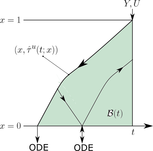
Figure 3: Schematic of the observer. First, the state on the characteristic line $(x,\hat{\tau}^{u}(t;x))$, $x\in[0,1]$ is estimated, starting with the measurement at $x=1$ and backwards relative to the propagation direction of $u$. Second, the current state is estimated by solving the system dynamics over the domain $\mathcal{B}(t)$ (shaded in green).

Sections 2 and 3 considered the case where the whole state $(w(\cdot,t),X(t))$ is available to the feedback controller, which is unrealistic in practical applications. Therefore, we present an observer that estimates both the distributed state $w(\cdot,t)$ and the ODE state $X(t)$ from the boundary measurement

$$Y(t)=u(1,t).$$ (61)

Like in [16], the observer design is based on the observation that the measurement $Y(t)$ contains only information about past values of the ODE state and the distributed state in the interior of the domain. For instance, the effect of any disturbance affecting $X$ would not be detectable in $Y$ for a certain amount of time. Therefore, we first estimate the past state on the characteristic line along which the measurement evolved, before mapping this estimate into an estimate of the current state via a prediction step. This two-step procedure is outlined in Figure 3. We again split the observer design into two cases depending on whether the speeds $\Lambda$ depend on the state or not.

Assumption 11.

There exists an observer $h$ for the ODE part of the system such that the state estimate $\hat{X}(t)$ satisfying

$$\dot{\hat{X}}(t) =h(\hat{X}(t),u(0,t),v(0,t),t),$$ (62)

$$\hat{X}(0) =\hat{X}_{0},$$ (63)

converges to the actual value $X(t)$ within finite time for any initial guess $\hat{X}_{0}$, input signal $v(0,t)$ and output measurement $u(0,t)$.

Some results on finite-time estimation of ODEs are given in [7, 15, 14].

Remark 12.

The assumption that the observer for the ODE part of the system converges within finite time is conservative and is made only so that it fits into the framework of exact estimation and exact predictions as in the state feedback case. Algorithmically, the implementation for the case where the observer for the ODE converges only asymptotically is exactly the same. However, any remaining estimation error would lead to prediction error when mapping the estimates $(\hat{w},\hat{X})$ into the estimate of the current state $(w,X)$ as described in Section 4.3. In the case with static boundary conditions, it was possible to show that the closed-loop system is robustly stable in presence of uncertainty in the boundary condition [21], and one might expect that something similar can be shown for the case considered here.

Define the characteristic line along which the measurement $Y(t)$ evolved and the past state on this line as

$$\check{\tau}^{u}(t;x) =t-\int_{x}^{1}\frac{1}{\lambda^{u}(\xi;w(\xi,\check{\tau}^{u}(t;\xi)))}d\xi,$$ (64)

$$\check{w}(x,t) =(\check{u},\check{v})(x,t)=w(x,\check{\tau}^{u}(t;x)),$$ (65)

$$\check{X}(t) =X(\check{\tau}^{u}(t;0)).$$ (66)

4.1 Estimation of $(\check{w},\check{X})$ - semilinear systems

If $\Lambda$ is independent of the state, one can show that, similar to [16, Theorem 8], $\check{w}$ satisfies

$$\check{u}_{x}(x,t) =\frac{f^{u}(x,\check{w}(x,t))}{\lambda^{u}(x)},$$ (67)

$$\check{v}_{t}(x,t) =\hat{\mu}(x)\,\check{v}_{x}(x,t)+\hat{\nu}(x)\,f^{v}(x,\check{w}(x,t)),$$ (68)

$$\dot{\check{X}}(t) =f^{0}(\check{X}(t),\check{v}(0,t),\check{\tau}^{u}(t;0)),$$ (69)

$$\check{u}(0,t) =g^{0}(\check{X}(t),\check{v}(0,t),\check{\tau}^{u}(t;0)),$$ (70)

$$\check{v}(1,t) =U(t),$$ (71)

where $\hat{\nu}=\frac{\lambda^{u}}{\lambda^{u}+\lambda^{v}}$ and $\hat{\mu}=\lambda^{v}\hat{\nu}$. Note that (67) is an ODE which can again be solved in either $x$-direction. The boundary value of $\check{u}$ at $x=1$ is known, whereas the boundary condition at $x=0$ given by (70) depends on $\check{X}$, which is yet to be estimated. Therefore, we design the observer as a copy (67)-(71) but with the boundary condition (70) replaced by the measurement, and the ODE (69) replaced by the observer from Assumption 11:

$$\hat{u}_{x}(x,t) =\frac{f^{u}(x,\hat{w}(x,t))}{\lambda^{u}(x)},$$ (72)

$$\hat{v}_{t}(x,t) =\hat{\mu}(x)\,\hat{v}_{x}(x,t)+\hat{\nu}(x)\,f^{v}(x,\hat{w}(x,t)),$$ (73)

$$\hat{u}(1,t) =Y(t),$$ (74)

$$\check{v}(1,t) =U(t),$$ (75)

$$\hat{w}(\cdot,0) =\hat{w}_{0},$$ (76)

$$\dot{\hat{X}}(t) =h(\hat{X}(t),\hat{u}(0,t),\hat{v}(0,t),\check{\tau}^{u}(t;0)),$$ (77)

$$\hat{X}(0) =\hat{X}_{0}.$$ (78)

Note that observer (72)-(78) has a cascade structure: The PDE state $\hat{w}$ is estimated via (72)-(76) without using the boundary condition at $x=0$ or $\hat{X}$ at all; then, the estimates of the unmeasured boundary values $(\hat{u}(0,t),\hat{v}(0,t))$ are used to estimate the ODE state $\hat{X}$ via (77)-(78). That is, the estimate $\hat{X}$ does not affect the estimate $\hat{w}$ at all. With this design, the estimates $(\hat{w},\hat{X})$ converge to the actual, past states $(\check{w},\check{X})$ within finite time.

Theorem 13.

There exists a $T>0$ such that for any initial guess $(\hat{w}_{0},\hat{X}_{0})$ and any $Y,U$ in $L^{\infty}$, we have $\hat{w}(\cdot,t)=\check{w}(\cdot,t)$ and $\hat{X}(t)=\check{X}(t)$ for all $t\geq T$.

The PDE-part of the observer, (72)-(76), converges to $\check{w}$ within finite time exactly as in the case with static boundary condition in [16, Theorem 19]. That is, within finite time one has exact estimates $(\hat{u}(0,t),\hat{v}(0,t))=(\check{u}(0,t),\check{v}(0,t))$, which are the inputs to the ODE-observer. Therefore, $\hat{X}$ converges to $\check{X}$ within another finite amount of time due to Assumption 11.

4.2 Estimation of $(\check{w},\check{X})$ - quasilinear systems

In quasilinear systems, the speed corresponding to $\hat{\mu}$ in (68) becomes time varying because the characteristic line $\check{\tau}^{u}$ depends on the state. Therefore, the observer additionally needs to estimate $\check{\tau}^{u}$ and its time-derivative. This is possible by designing the observer as a copy of the dynamics of $\check{w}$ up to the first time-derivatives (in a manner similar to (47)-(59)), and again imposing the measurements and its time-derivative as a boundary value at $x=1$ instead of using the to-be estimated boundary condition at $x=0$. We estimate the PDE state via

$$\partial_{x}\hat{u}(x,t)= \ \frac{f^{u}}{\lambda^{u}},$$ (79)

$$\partial_{t}\hat{v}(x,t)= \ \partial_{t}\hat{\tau}^{u}\times\left(\hat{\mu}\times\partial_{x}\hat{v}(x,t)+\hat{\nu}\times f^{v}\right)$$ (80)

$$\partial_{x}\hat{u}_{\partial t}(x,t)= \ \frac{1}{\lambda^{u}}\times\left[c_{1}\,(\hat{u}_{\partial t})^{2}+c_{2}\,\hat{u}_{\partial t}\,\hat{v}_{\partial t}\right.$$

$$\left.~{}~{}~{}~{}~{}~{}~{}~{}~{}+c_{3}\,\hat{u}_{\partial t}+c_{4}\,\hat{v}_{\partial t}\right],$$ (81)

$$\partial_{t}\hat{v}_{\partial t}(x,t)= \ \partial_{t}\hat{\tau}^{u}\times\left(\hat{\mu}\times\partial_{x}\hat{v}_{\partial t}(x,t)+\hat{\nu}\times\left[c_{5}\,\hat{u}_{\partial t}\,\hat{v}_{\partial t}\right.\right.$$

$$~{}~{}~{}~{}\left.\left.+c_{6}\,(\hat{v}_{\partial t})^{2}+c_{7}\,\hat{u}_{\partial t}+c_{8}\,\hat{v}_{\partial t}\right]\right),$$ (82)

$$\hat{\tau}^{u}(t;x)= \ t-\int_{x}^{1}\frac{1}{\lambda^{u}(\xi;\hat{w}(\xi,t))}d\xi$$ (83)

$$\partial_{t}\hat{\tau}^{u}(t;x)= \ 1+\int_{x}^{1}\frac{\partial_{u}\lambda^{u}\times\hat{u}_{\partial t}+\partial_{v}\lambda^{u}\times\hat{v}_{\partial t}}{\left(\lambda^{u}\right)^{2}}d\xi,$$ (84)

$$\hat{u}(1,t)= \ Y(t),$$ (85)

$$\hat{u}_{\partial_{t}}(1,t)= \ \partial_{t}Y(t),$$ (86)

$$\hat{v}(1,t)= \ U(t),$$ (87)

$$\hat{v}_{\partial_{t}}(1,t)= \ \partial_{t}U(t),$$ (88)

and the ODE state via

$$\dot{\hat{X}}(t)=\partial_{t}\hat{\tau}^{u}(t;0)\times h(\hat{X}(t),\hat{u}(0,t),\hat{v}(0,t),\hat{\tau}^{u}(t;0)),$$ (89)

with initial guesses

$$\hat{w}(\cdot,0) =\hat{w}_{0}, \hat{v}_{\partial t}(\cdot,0) =\hat{v}_{\partial t}^{0}, \hat{X}(0) =\hat{X}_{0}.$$ (90)

Similar to the semilinear case, this observer converges in finite time.

Theorem 14.

There exist $\epsilon^{\prime}>0$ (which depends on $\max\{\|\hat{w}_{0}\|_{\infty},\|Y\|_{\infty},\|U\|_{\infty}\}$) and $T>0$ such that if $\|\hat{v}_{\partial t}^{0}\|_{\infty}\leq\epsilon^{\prime}$, $\|\partial_{t}Y\|_{\infty}\leq\epsilon^{\prime}$ and $\|\partial_{t}U\|_{\infty}\leq\epsilon^{\prime}$, then $\hat{w}(\cdot,t)=\check{w}(\cdot,t)$ and $\hat{X}(t)=\check{X}(t)$ for all $t\geq T$.

Convergence follows exactly as in the semilinear case in Theorem 13. Smallness of $\hat{v}_{\partial t}^{0}$, $\partial_{t}Y$ and $\partial_{t}U$ is sufficient for preventing blow-up of the estimate $\hat{w}$. This can be shown using the concept of semi-global solutions as in [21, Theorems 3 and 4]. Briefly, the characteristic lines of (79)-(90) all start at either $x=1$ or $t=0$ and all go in the negative $x$-direction. Consequently, (79)-(90) (excluding the part involving $X$) can be seen as an PDE-ODE system in the negative $x$-direction, and conditions like in Lemma 9 or [21, Theorem 4] can be applied to ensure existence of a solution for $\hat{w}$ on the bounded $x$-horizon $x\in[0,1]$. The estimate of the ODE state, $\hat{X}$, does not blow up and it converges due to Assumption 11.

4.3 Estimation of current state and output feedback

The observers presented above only estimate the past state $(\check{w},\check{X})$ as defined in (65)-(66). That estimate of the past state can be mapped to an estimate of the current state, at time $t$, through another prediction step by solving the system dynamics with initial condition given by $(\hat{w},\hat{X})$, i.e.,

$$w^{\mathrm{est}}_{t}(x,s) =\Lambda(x,w^{\mathrm{est}}(x,s))\,w^{\mathrm{est}}_{x}(x,s)$$

$$\qquad+F(x,w^{\mathrm{est}}(x,s)),$$ (91)

$$\dot{X}^{\mathrm{est}}(s) =f^{0}(X^{\mathrm{est}}(s),v^{\mathrm{est}}(0,s),s),$$ (92)

$$u^{\mathrm{est}}(0,s) =g^{0}(X^{\mathrm{est}}(s),v^{\mathrm{est}}(0,s),s),$$ (93)

$$w^{\mathrm{est}}(\cdot,\hat{\tau}^{u}(t;\cdot)) =\hat{w}(\cdot,t),$$ (94)

$$X^{\mathrm{est}}(\hat{\tau}^{u}(t;0)) =\hat{X}(t),$$ (95)

over the domain

$$\mathcal{B}(t) =\left\{(x,s):\,x\in[0,1],\,s\in[\hat{\tau}^{u}(t;x),t]\right\},$$ (96)

where $\hat{\tau}^{u}$ can be replaced by $\check{\tau}^{u}$ in the semilinear case. Similar to Lemmas 2 and 8, and assuming in the quasilinear case that $\hat{w}_{0}$, $\hat{X}_{0}$, $Y$ and $U$ have sufficiently small infinity-norm, system (91)-(95) has a unique solution on $\mathcal{B}(t)$. By virtue of Theorems 13 and 14, this implies that $(w^{\mathrm{est}}(\cdot,t),X^{\mathrm{est}}(t))=(w(\cdot,t),X(t))$ for all $t\geq T$ for some sufficiently large, but finite $T$.

This observer can be combined with the state feedback controllers from Sections 2 and 3, respectively, to obtain the corresponding output feedback controller that uses only the boundary measurement $Y$ as defined in (61). In the semilinear case, the point $x=1$ can be left out of the domain $\mathcal{B}(t)$ when solving (91)-(95) because the control input $U(t)$ is not yet known when the observer is evaluated. Omitting this one point has no influence on the solution of (39) when the control input is constructed. In the quasilinear case, smallness of $U$, $Y$ and their derivatives is also required. This can be guaranteed if $\|w_{0}\|_{\infty}$, $\|X_{0}\|_{\infty}$ and $\|\partial_{x}w_{0}\|_{\infty}$ are sufficiently small, and $\|\hat{w}_{0}\|_{\infty}$, $\|\hat{X}_{0}\|_{\infty}$, $\|\partial_{x}\hat{w}_{0}\|_{\infty}$ as well as $\delta$ in (46) are chosen sufficiently small. This can be shown via analysis of the worst-case growth of the time derivatives as performed in [21]. In practice it makes sense, depending on the application, to activate the controller only once the observer has had time to converge to the actual state.

The observer presented here is somewhat related to the one from [13] for systems with static boundary conditions, in that it provides exact state estimates within the same time. However, in the approach from [13], the estimate of the past state in the interior of the domain is obtained by saving the history of boundary measurements and solving another PDE. Whereas in the approach presented here, the observers (72)-(78) or (79)-(90), respectively, estimate $(\check{w},\check{X})$ dynamically without the need for saving any measurements.

5 Simulation example

We demonstrate the performance of the proposed controller in numerical simulations of a system with $n=1$ and the parameters

$$f^{u} =\sin(u+v), f^{v} =\sin(v-u),$$ (97)

$$\lambda^{u} =\begin{cases}0.5&x<0.5\\ x&x\geq 0.5\end{cases}, \lambda^{u} =1+0.5\times(|u|+|v|),$$ (98)

$$f^{0} =X|X|+v(0,t), g^{0} =X+v(0,t),$$ (99)

$$v_{0} =0.5\times(1+x), u_{0} =-0.5,$$ (100)

$$X_{0} =-1.$$ (101)

The sampling time is set to $\theta=0.5$ and the convergence speed to $\delta=1$. For simplicity, we consider the state-feedback case. As in [21], the simulation and controller are implemented by first semi-discretizing all PDEs in space using finite differences. The resulting high-order ODEs are then solved in Matlab by use of ode45. For a discretization with 100 spatial elements, which has been used to produce the figures, evaluating the controller takes around $0.1$ seconds on a standard laptop, although the code has not been optimized for performance.

Stabilization

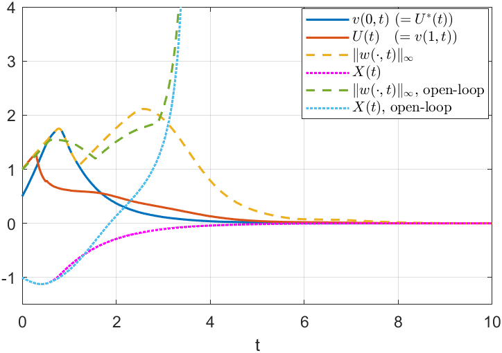
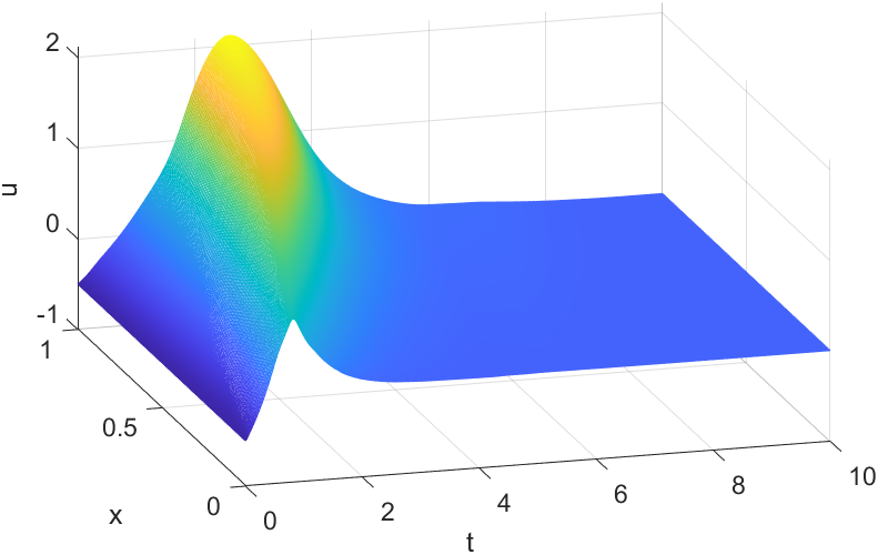
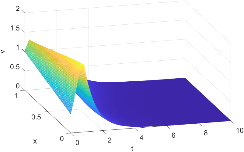
Figure 4: Trajectories of the stabilization (top) and tracking (bottom) examples. The top left figure also shows the state norm and trajectory of $X$ for the open-loop case where the control input is held constant at $U(t)=1$.

Figure 4 shows the trajectories when the controller

$$K=-X|X|-X$$ (102)

is used. Clearly, the term $-X|X|$ is designed to cancel the destabilizing nonlinearity in $f^{0}$, while the term $-X$ is used to drive the system to the origin. In accordance with theory, after some transients the system asymptotically converges to the origin. For comparison, Figure 4 also shows the trajectories of $X$ and $\|w(\cdot,t)\|_{\infty}$ for the case where the system is run in open loop with $U(t)=1$ for all times. For this constant input, the solution escapes in finite time at around $t=3.6$.

Reference tracking  The control design presented in this paper can be modified to achieve tracking of a reference signal $X_{ref}$. If tracking is the control objective, it is not necessary to assume that the origin is an equilibrium, i.e., assumptions (15)-(16) and (18) can be dropped. For this purpose, the ODE controller is changed to

$$K=-X|X|+2\times(X_{ref}(t)-X).$$ (103)

That is, the controller becomes time-varying. Like before, the term $-X|X|$ is to cancel the destabilizing nonlinearity and the second term $2\times(X_{ref}(t)-X)$ is designed to achieve reference tracking. The simulated trajectories are shown in the bottom row of Figure 4. The controller achieves good reference tracking and the solution of remains bounded at all times.

6 Conclusions

We generalized a recently developed boundary controller for $2\times 2$ quasilinear hyperbolic systems to the case where the same type of PDE is coupled with an ODE at the uncontrolled boundary. Based on predictions over the maximum determinate sets, it is possible to treat the future control input to the ODE subsystem as an virtual input, before the actual inputs are computed by feeding the virtual inputs through the inverted PDE dynamics. A detailed comparison of semilinear and general quasilinear systems is given. In particular, the control inputs can be chosen more freely in the semilinear case and less attention needs to be put into ensuring that the solution does not blow up in finite time.

It is noteworthy that the generalization from $2\times 2$ hyperbolic systems with static boundary conditions to systems coupled with an ODE is relatively straightforward despite the complex dynamics. Some other variations that have been published in the past for semilinear systems, such as to a linear network structure [17] and to bilateral control [18], have also been without major complications once the design for basic $2\times 2$ hyperbolic systems was known. Overall, these results demonstrate the flexibility of the approach.

We also presented an observer that estimates the distributed PDE state and the unmeasured ODE state from measurements at the actuated boundary only. The observer has a cascade structure, where the PDE state is estimated independently of the estimate of the ODE state, but the estimate of the PDE state is used to estimate the ODE state. This structure can be exploited if the hyperbolic PDE is coupled to a different type of system, such as another PDE. Another situation of interest might be $2\times 2$ hyperbolic PDEs coupled to an uncertain ODE. If, for instance, an adaptive observer existed for the ODE itself (without the coupling to the PDE), it is straightforward to include such an adaptive observer in the design presented here, although rigorous conditions for existence of the solutions might be challenging.

References

- [1] Georges Bastin and Jean-Michel Coron. Stability and boundary stabilization of 1-d hyperbolic systems, volume 88. Springer, 2016.
- [2] Alberto Bressan. Hyperbolic systems of conservation laws: the one-dimensional Cauchy problem, volume 20. Oxford University Press, 2000.
- [3] Jean-Michel Coron, Brigitte d’Andrea Novel, and Georges Bastin. A strict Lyapunov function for boundary control of hyperbolic systems of conservation laws. IEEE Transactions on Automatic Control, 52(1):2–11, 2007.
- [4] Jean-Michel Coron, Rafael Vazquez, Miroslav Krstic, and Georges Bastin. Local exponential stabilization of a quasilinear hyperbolic system using backstepping. SIAM Journal on Control and Optimization, 51(3):2005–2035, 2013.
- [5] F Di Meglio and UJF Aarsnes. A distributed parameter systems view of control problems in drilling. In 2nd IFAC Workshop on Automatic Control in Offshore Oil and Gas Production, Florianópolis, Brazil, 2015.
- [6] Florent Di Meglio, Federico Bribiesca Argomedo, Long Hu, and Miroslav Krstic. Stabilization of coupled linear heterodirectional hyperbolic pde–ode systems. Automatica, 87:281–289, 2018.
- [7] Robert Engel and Gerhard Kreisselmeier. A continuous-time observer which converges in finite time. IEEE Transactions on Automatic Control, 47(7):1202–1204, 2002.
- [8] James M Greenberg and Ta-Tsien Li. The effect of boundary damping for the quasilinear wave equation. Journal of Differential Equations, 52(1):66–75, 1984.
- [9] Martin Gugat and Günter Leugering. Global boundary controllability of the de St. Venant equations between steady states. In Annales de l’IHP Analyse non linéaire, volume 20, pages 1–11, 2003.
- [10] Miroslav Krstic and Andrey Smyshlyaev. Backstepping boundary control for first-order hyperbolic PDEs and application to systems with actuator and sensor delays. Systems & Control Letters, 57(9):750–758, 2008.
- [11] Ta-Tsien Li and Bo-Peng Rao. Exact boundary controllability for quasi-linear hyperbolic systems. SIAM Journal on Control and Optimization, 41(6):1748–1755, 2003.
- [12] Ta-Tsien Li, Bopeng Rao, and Yi Jin. Semi-global solution and exact boundary controllability for reducible quasilinear hyperbolic systems. ESAIM: Mathematical Modelling and Numerical Analysis, 34(2):399–408, 2000.
- [13] Tatsien Li. Exact boundary observability for quasilinear hyperbolic systems. ESAIM: Control, Optimisation and Calculus of Variations, 14(4):759–766, 2008.
- [14] Francisco Lopez-Ramirez, Andrey Polyakov, Denis Efimov, and Wilfrid Perruquetti. Finite-time and fixed-time observer design: Implicit lyapunov function approach. Automatica, 87:52–60, 2018.
- [15] Tomas Menard, Emmanuel Moulay, and Wilfrid Perruquetti. A global high-gain finite-time observer. IEEE Transactions on automatic control, 55(6):1500–1506, 2010.
- [16] Timm Strecker and Ole Morten Aamo. Output feedback boundary control of semilinear hyperbolic systems. Automatica, 83:290–302, 2017.
- [17] Timm Strecker and Ole Morten Aamo. Output feedback boundary control of series interconnections of semilinear hyperbolic systems. In 20th IFAC World Congress, 2017. IFAC, 2017.
- [18] Timm Strecker and Ole Morten Aamo. Two-sided boundary control and state estimation of semilinear hyperbolic systems. In 2017 IEEE 56th Annual Conference on Decision and Control (CDC), pages 2511–2518. IEEE, 2017.
- [19] Timm Strecker, Ole Morten Aamo, and Michael Cantoni. Direct predictive boundary control of a first-order quasilinear hyperbolic PDE. In 2019 IEEE 58th Annual Conference on Decision and Control (CDC). IEEE, 2019.
- [20] Timm Strecker, Ole Morten Aamo, and Michael Cantoni. Output feedback boundary control of heterodirectional semilinear hyperbolic systems. Automatica, 117:108990, 2020.
- [21] Timm Strecker, Ole Morten Aamo, and Michael Cantoni. Boundary feedback control of quasilinear hyperbolic systems: Predictive synthesis and robustness analysis. Accepted for publication in IEEE Transactions on Automatic Control. Available: https://arxiv.org/abs/2104.04581, 2021.
- [22] Rafael Vazquez, Miroslav Krstic, and Jean-Michel Coron. Backstepping boundary stabilization and state estimation of a 2 2 linear hyperbolic system. In 2011 50th IEEE Conference on Decision and Control and European Control Conference (CDC-ECC), pages 4937–4942, 2011.