PT symmetry and the evolution speed in open quantum systems

Abstract

The dynamics of an open quantum system with balanced gain and loss is not described by a PT-symmetric Hamiltonian but rather by Lindblad operators. Nevertheless the phenomenon of PT-symmetry breaking and the impact of exceptional points can be observed in the Lindbladean dynamics. Here we briefly review the development of PT symmetry in quantum mechanics, and the characterisation of PT-symmetry breaking in open quantum systems in terms of the behaviour of the speed of evolution of the state.

1 PT symmetry and quantum physics

We begin with a brief account of the development of PT symmetry in quantum mechanics. In 1998 Bender and Boettcher found that there is a family of Hamiltonians of the form ${\hat{H}}=\frac{1}{2}{\hat{p}}^{2}+{\hat{x}}^{2}({\rm i}{\hat{x}})^{\epsilon}$ that possesses real, positive, and discrete eigenvalues for all $\epsilon\geq 0$ [1]. These Hamiltonians, while not Hermitian, are nevertheless invariant under the action of parity-and-time (PT) reversal: ${\hat{p}}\to{\hat{p}}$, ${\hat{x}}\to-{\hat{x}}$, and ${\rm i}\to-{\rm i}$. This observation led them to conjecture that generic PT-symmetric Hamiltonians may possess entirely real eigenvalues. Subsequently, eigenvalues of many other PT-symmetric Hamiltonians were investigated by numerous authors.

A natural question thus arising is whether a consistent quantum theory can be developed by use of a PT-symmetric Hamiltonian. In standard quantum mechanics the reality of observables are ensured by the Hermiticity condition on the Hilbert space endowed with a Hermitian inner product. While Hermiticity may be replaced by the condition of PT symmetry to enforce the reality of observables, a Hilbert space endowed with a PT-conjugation inner product is problematic, for, the parity operator is trace free and squares to the identity so that half of its eigenvalues are negative. In other words, such Hilbert spaces are of the Pontryagin-type that come equipped with indefinite metrics [2]. Because Hilbert-space norms are related to probabilities in quantum mechanics, negative norms would imply negative probabilities, which makes the theory unphysical.

In 2002, however, Mostafazadeh [3], and independently Bender at al. [4] observed that for a PT-symmetric Hamiltonian ${\hat{H}}$ there exists another PT-symmetric observable that commutes with ${\hat{H}}$ such that its eigenvalues are either plus or minus one, depending on the parity type of the eigenfunctions of ${\hat{H}}$. Such an operator naturally has the interpretation analogous to a charge (C) operator. This means that a PT-symmetric Hamiltonian is automatically CPT-symmetric, so in fact we can speak of CPT-symmetric quantum theory for which the Hilbert-space inner product is defined with respect to a positive-definite CPT conjugation. In particular, writing ${\hat{g}}$ for the operator associated with the CP conjugation, the inner product of a pair of elements $|\psi\rangle$ and $|\varphi\rangle$ is given by $\langle\psi,\varphi\rangle=\langle\psi|{\hat{g}}|\varphi\rangle$. It can then be shown that the operator ${\hat{g}}$ is Hermitian and positive, so that it admits the interpretation of defining a metric on Hilbert space, and thus is sometimes referred to as the metric operator.

Because ${\hat{g}}$ is Hermitian and positive, there is an operator ${\hat{u}}$, not unique, such that we can write ${\hat{g}}={\hat{u}}{\hat{u}}^{\dagger}$. Then the operator ${\hat{u}}$ can be used to map between the Hilbert space endowed with a standard Hermitian inner product and that endowed with a CPT inner product, because $\langle\psi,\varphi\rangle=\langle{\hat{u}}^{\dagger}\psi|{\hat{u}}^{\dagger}\varphi\rangle$. Further, the operator ${\hat{u}}$ can be used to define a similarity transformation between a PT-symmetric observable and a Hermitian observable; whereas ${\hat{g}}$ can be used to determine the Hermitian adjoint of an observable ${\hat{F}}$ in the sense that ${\hat{F}}^{\dagger}={\hat{g}}^{-1}{\hat{F}}{\hat{g}}$. An operator satisfying such a condition is sometimes referred to as being ‘pseudo-Hermitian’. Once these structures associated with PT symmetry were uncovered, it became appreciated that the notion of pseudo-Hermiticity in itself has been around for some time [5], and likewise the idea of defining Hilbert space inner product in terms of a nontrivial metric operator for characterising quantum theory has been proposed previously [6], albeit in a different context.

The fact that there is a similarity transformation relating a PT-symmetric Hamiltonian to a Hermitian one naturally raises the question whether a quantum system described by a PT-symmetric Hamiltonian is in fact equivalent to standard Hermitian quantum mechanics. That they are indeed equivalent on account of the existence of a similarity transformation is the point that has been argued for long by Mostafazadeh [7], although in infinite dimensions one has to be cautious in making such an assertion.

To discuss the question of equivalence it will be useful first to consider quantum systems modelled on finite-dimensional Hilbert spaces. In this case, all operators are bounded, so mathematical subtleties associated with unbounded operators do not enter the discussion. It is then tempting to conclude that a system described by a PT-symmetric Hamiltonian is just an alternative representation of the same system described by a Hermitian Hamiltonian, i.e. they are equivalent. This ‘equivalence’ argument by itself does not quite account for exactly what goes on for two reasons: First, a PT-symmetric Hamiltonian admits more parametric degrees of freedom than a Hermitian Hamiltonian. For instance, in the case of a two-level system, a Hermitian Hamiltonian has four independent parameters, while a PT-symmetric Hamiltonian can have six independent parameters. More generally, for an $n$-level system a PT-symmetric Hamiltonian can have $n(2n-1)$ independent parameters, as opposed to $n^{2}$ for a Hermitian Hamiltonian. Because parameters in a Hamiltonian represent experimental setup, a blind statement of equivalence does not explain this discrepancy. Second, for a PT-symmetric Hamiltonian it is possible to vary parameters in the Hamiltonian to effect a phase transition for which in one phase the eigenstates of the Hamiltonian are PT symmetric (the unbroken phase), while in the other, broken phase they are not. In the broken phase, the eigenvalues of the Hamiltonian are no longer real—some, or all of them, come in complex conjugate pairs. No such phenomenon is seen in a Hermitian Hamiltonian in finite dimensions.

This apparent contradiction was further clarified in 2016 when it was shown, using a biorthogonal formalism of [8], that there is a canonical separation of the degrees of freedom in a PT-symmetric Hamiltonian into two sets: one corresponding to the degrees of freedom associated with its Hermitian counterpart Hamiltonian, and one corresponding to the degrees of freedom associated with the specification of the metric operator ${\hat{g}}$ [9]. Further, it was shown that for closed quantum systems there are no laboratory experiments to adjust or determine the values of the latter degrees of freedom. That is, the expectation values of physical observables are independent of ${\hat{g}}$. Thus, perhaps a better characterisation is that for a finite-dimensional system the two descriptions are indistinguishable rather than equivalent. In particular, without the ability to adjust the parameters in the operator ${\hat{g}}$ it is not possible to experimentally realise the phase transition discussed above.

In the infinite-dimensional case, the situation is more complicated even in the countable case, because the equivalence of eigenvalues between a PT-symmetric Hamiltonian and its Hermitian ‘counterpart’ Hamiltonian related by a similarity transformation involving the operator ${\hat{g}}$ is ensured only if both operators ${\hat{g}}$ and ${\hat{g}}^{-1}$ are bounded. Otherwise, the image of an eigenstate of one of the Hamiltonians under the map, or more generally the image of any state from the domain of this Hamiltonian, may not belong to the other Hilbert space, or to the domain of the other Hamiltonian. For many model Hamiltonians studied in the literature, either ${\hat{g}}$ or ${\hat{g}}^{-1}$ (or both) are unbounded, and in these cases it is not simple to determine whether the two descriptions are equivalent: It may be the case that there are genuinely new physics of closed quantum systems modelled on infinite-dimensional Hilbert spaces, possibly with a partially broken PT symmetry, although this remains to be further investigated.

The above discussion is concerned with closed systems. Around 2006, however, it was observed that PT symmetry can be realised in a laboratory for open systems by balancing gain and loss [10, 11, 12]. For example, suppose that with respect to a choice of reference frame the left side of the system absorbs energy, while the right side emits energy, in a symmetric configuration, by the same amount. Then under parity (left-right) reversal, gain turns into loss and loss turns into gain; but time reversal has the same effect so that the system is PT symmetric. Intuitively, although the system is open, it can behave in a manner similar to a closed one because the overall energy is conserved. Such an open system can thus be described by a PT-symmetric Hamiltonian, where now the degrees freedom associated with the operator ${\hat{g}}$ can be controlled in a laboratory by adjusting, for instance, the gain and loss strengths. It should be evident, however, that for such a system to remain in a quasi-equilibrium state of energy, the internal energy transport, i.e. the coupling strength of the left and the right side of the system, has to be sufficiently strong, for otherwise the system cannot redistribute the energy to maintain its quasi-equilibrium state. Thus by increasing gain and loss strengths while keeping the internal interaction strength fixed, the system undergoes a phase transition such that although the Hamiltonian remains PT symmetric, its eigenstates are no longer PT symmetric and consequently the energy eigenvalues become complex. For PT-symmetric systems, such transitions are accompanied by the degeneracies of the energy eigenstates, and these critical points are often referred to as exceptional points in the literature [13, 14, 15, 16, 17].

The facts that PT symmetry can be implemented relatively straightforwardly for open systems in a laboratory, and that such systems typically exhibit nontrivial phase transitions with interesting and sometimes counterintuitive features, led many researchers to explore properties of PT-symmetric systems both theoretically and experimentally—perhaps most notably in the context of optical systems such as optical waveguides. In the context of open systems, however, those whose dynamics are described by PT-symmetric Hamiltonians are classical rather than quantum mechanical. Likewise, many of the experiments that were implemented concern classical systems. The reason is because a perfect balancing of gain and loss of energy (or of particle number, or of volume) is not feasible in quantum mechanics.

To see this, it suffices to consider the simple system described above where energy is absorbed on the left side and emitted on the right side. Suppose that $\epsilon$ joules of energy is absorbed on the left side between time $t$ and time $t+{\rm d}t$ where ${\rm d}t\ll 1$. Then to perfectly balance this, it is necessary that exactly $\epsilon$ joules of energy is emitted from the right side precisely over the same time interval. Such a process can be achieved classically. Quantum mechanically, to realise a perfect PT symmetry one requires a sharp precision in both energy and time, but such a precision amounts to violating the energy-time uncertainty relation. Another way of seeing the issue is to consider a quantum system having a discrete set of energy eigenvalues. Then unless the eigenvalues are equally spaced (such as an oscillator) and the value of $\epsilon$ coinciding with the energy gap, the system will always remain in a state of indefinite energy (i.e. not an energy eigenstate) and one can only consider the expectation value of the Hamiltonian in order to speak about the energy of the system.

The impossibility of maintaining a perfect PT symmetry, however, does not mean that a PT-symmetric open environment cannot be realised in quantum mechanics, because it remains meaningful to speak about balancing gain and loss on average. A PT-symmetric configuration of the absorption and emission rates does not violate Heisenberg constraints. However, the fact that one cannot determine whether the system has, say, absorbed or emitted energy, implies that as time passes, the observer gradually loses information about the state of the system. The theoretical implication is that it is not possible to characterise the dynamics of a PT-symmetric open quantum system in terms of a PT-symmetric Hamiltonian. Instead, time evolution is governed by an equation of the Lindblad type, or more generally of the Krauss type.

Focusing in particular on systems described by the Lindblad equation, it would be of interest then to enquire what are the characteristic features of PT-symmetric open quantum systems and the associated symmetry breaking. Indeed, there are growing interests in studying the effects of exceptional points in genuinely open quantum systems described by Lindblad equations [18, 19]. With this in mind, the purpose here is to explore this question by focusing specifically on the behaviour of the speed of the evolution of the state that has been examined in [20].

2 Open quantum system dynamics

Intuitively, by an open system $S$ we have in mind one that is coupled to another system $B$. The latter may be large enough to act as a bath, or may be another small quantum system. Suppose that the total system $S+B$ is described by a pure-state wave function $|\Psi_{S+B}\rangle$. The state of an open quantum system $S$ is then determined by tracing out the degrees of freedom associated with $B$:

$${\hat{\rho}}_{S}={\rm tr}_{B}\left(\frac{|\Psi_{S+B}\rangle\langle\Psi_{S+B}|}{\langle\Psi_{S+B}|\Psi_{S+B}\rangle}\right).$$

Provided that the state $|\Psi_{S+B}\rangle$ is not a product state of the form $|\Psi_{S+B}\rangle=|\Psi_{S}\rangle\otimes|\Psi_{B}\rangle$, or equivalently stated if the two systems $S$ and $B$ are entangled, the result of the tracing is necessarily a mixed-state density matrix so that we have ${\hat{\rho}}_{S}^{2}\neq{\hat{\rho}}_{S}$. As an example, suppose that $S$ and $B$ are both spin-$\frac{1}{2}$ particles, and $|\Psi_{S+B}\rangle$ is the pure spin-0 singlet state $\frac{1}{\sqrt{2}}(|\!\uparrow\downarrow\rangle-|\!\downarrow\uparrow\rangle)$. Then tracing over $B$ we obtain

$${\hat{\rho}}_{S}=\mbox{$\textstyle\frac{1}{2}$}\big{(}|\!\uparrow\rangle\langle\uparrow\!|+|\!\downarrow\rangle\langle\downarrow\!|\big{)},$$

which is a state distinct from the coherent superposition $\frac{1}{\sqrt{2}}(|\!\uparrow\rangle+|\!\downarrow\rangle)$.

We can think of a density matrix as representing a (classical) statistical average over pure states, in the sense that it can be written as the expectation of a random pure-state projection operator:

$${\hat{\rho}}={\mathbb{E}}\left[\frac{|\psi\rangle\langle\psi|}{\langle\psi|\psi\rangle}\right].$$

For instance, suppose that an experimentalist is aware that the state of the system will be $|\psi_{1}\rangle$ if the system absorbs energy, but otherwise will be $|\psi_{0}\rangle$, and that the probability of absorption is $p$. Then without a measurement to acquire more information (and thus altering the state) one can only assert that the system is in the averaged state

$${\hat{\rho}}=p\frac{|\psi_{1}\rangle\langle\psi_{1}|}{\langle\psi_{1}|\psi_{1}\rangle}+(1-p)\frac{|\psi_{0}\rangle\langle\psi_{0}|}{\langle\psi_{0}|\psi_{0}\rangle},$$

which again is not the same state as the pure state $|\psi\rangle=\sqrt{p}\,|\psi_{1}\rangle+\sqrt{1-p}\,|\psi_{0}\rangle$. Thus the density matrix ${\hat{\rho}}$ has the interpretation of ‘either $|\psi_{0}\rangle$ or $|\psi_{1}\rangle$’ in the sense of classical probability, whereas the pure state $|\psi\rangle$ has the interpretation of ‘neither $|\psi_{0}\rangle$ nor $|\psi_{1}\rangle$’ in the sense of quantum probability; and the two states are experimentally distinguishable. A mixed state density matrix can always be expressed in such an ensemble average of pure states. However, given a state ${\hat{\rho}}$ there are uncountably many ways of expressing it in terms of averages of pure states, so it is not possible to determine which experimental setup has resulted in that state.

The time evolution of the density matrix that preserves its positivity and the trace condition can typically be described by the dynamical equation of the Lindblad type:

$$\partial_{t}{\hat{\rho}}=-{\rm i}[{\hat{H}},{\hat{\rho}}]+\sum_{k}\left[{\hat{L}}_{k}{\hat{\rho}}{\hat{L}}^{\dagger}_{k}-\frac{1}{2}\left({\hat{L}}^{\dagger}_{k}{\hat{L}}_{k}\rho+{\hat{\rho}}{\hat{L}}^{\dagger}_{k}{\hat{L}}_{k}\right)\right].$$

This is the so-called GKLS equation of Gorini, Kossakowski, Sudarshan [21] and Lindblad [22], or just the Lindblad equation for short. Interestingly, in the context of a proposal of Hawking [23] that the dynamical equation for the density matrix will in general not preserve unitarity, Banks, Susskind and Peskin [24] independently explored a general dynamics for the state that preserves positivity and trace condition, and arrived at an analogous dynamical equation satisfied by the density matrix.

The Lindblad operators ${\hat{L}}_{k}$ characterise the way in which the system $S$ interacts with the environment $B$. So for example if there is a particle gain at the left side and particle loss at the right side, then the dynamics of this system can be characterised by a pair of Lindblad operators with ${\hat{L}}_{1}=\gamma_{L}{\hat{a}}_{L}^{\dagger}$ and ${\hat{L}}_{2}=\gamma_{R}{\hat{a}}_{R}$, expressed in terms of the particle creation and annihilation operators, where the parameters $\gamma_{L},\gamma_{R}$ determine the gain/loss strengths. That an averaged balancing of gain and loss can be realised in this way to describe a PT-symmetric quantum system in the context of Bose-Einstein condensates has been known for long to the Stuttgart group [25, 26]. In the case of a many body system, such a system can be treated effectively in terms of a mean-field approximation, which in turn may be described by an effective PT-symmetric Hamiltonian [27].

From the linearity of the dynamics we can think of the right side of the Lindblad equation as representing the action of a Liouville operator ${\cal L}$ on ${\hat{\rho}}$, and write

$$\partial_{t}{\hat{\rho}}={\cal L}{\hat{\rho}}.$$

Here the Liouville operator ${\cal L}$ can be interpreted as a superoperator, which becomes evident if we express operators using the index notation by writing $\partial_{t}\rho^{\alpha}_{\beta}={\cal L}^{\alpha\alpha^{\prime}}_{\beta\beta^{\prime}}\rho^{\beta^{\prime}}_{\alpha^{\prime}}$ with repeated indices summed over. It turns out that the eigenvalues of ${\cal L}$ are real or else come in complex conjugate pairs, just like any PT-symmetric operator. Thus, from a certain point of view one could argue that every open system dynamics is PT symmetric, although exactly what that might mean physically is not well understood.

3 Unitary evolution speed for quantum states

There are various features of the dynamics of an open system that one can investigate, but following [20], here we shall be focused on one particular aspect concerning the speed of evolution of the state. The evolution speed of a quantum system in itself is of interest for several reasons. For example, to implement a quantum operation such as a quantum algorithm in a quantum computer, it is useful to have an idea on how fast a given task can be realised. The evolution speed is also linked to the sensitivity or stability of the state against changes in time, which in turn is useful in arriving at error lower bounds in estimating quantum states [28].

For pure states, the evolution speed under a unitary motion is given by the Anandan-Aharonov relation [29]. The idea can be described as follows. We start with the Schrödinger-Kibble equation

$$\frac{{\rm d}}{{\rm d}t}\,|{\psi}(t)\rangle=-{\rm i}\frac{1}{\hbar}\left({\hat{H}}-\langle\psi(t)|{\hat{H}}|\psi(t)\rangle\right)|\psi(t)\rangle$$

for the dynamics of the state. Note that the Schrödinger-Kibble equation is a nonlinear differential equation defined on Hilbert space. However, because the energy expectation $E=\langle\psi(t)|{\hat{H}}|\psi(t)\rangle$ is a constant of motion, the equation is indeed linear along each unitary orbit. The effect of removing the energy expectation from the Hamiltonian is to eliminate dynamical phase under the evolution, and the equation has the advantage that for a stationary state we have $|{\dot{\psi}}(t)\rangle=0$ and hence we automatically recover the time-independent Schrödinger equation ${\hat{H}}|\psi\rangle=E|\psi\rangle$, which in undergraduate quantum mechanics texts can only be derived by evoking the somewhat mysterious correspondence between energy and time derivative. Mathematically, the Schrödinger-Kibble equation gives what is called a horizontal lift of the Schrödinger equation in Hilbert space to the projective Hilbert space where the tangent vector $|\dot{\psi}\rangle$ is everywhere orthogonal to $|\psi\rangle$.

If the state $|\psi\rangle$ of a system satisfies the Schrödinger-Kibble equation, then the squared speed of evolution is determined by

$$v^{2}(t)=4\langle{\dot{\psi}}(t)|{\dot{\psi}}(t)\rangle,$$

where the factor of $4$ here is conventional in fixing the scale of the metric, and is related to the fact that the Bloch sphere of spin-$\frac{1}{2}$ systems has radius $\frac{1}{2}$. Alternatively, if we work with the solutions to the conventional Schrödinger equation $|{\dot{\psi}}(t)\rangle=-{\rm i}\hbar^{-1}{\hat{H}}|\psi(t)\rangle$, then we can define the proper ‘velocity’ vector by

$$|v(t)\rangle=|{\dot{\psi}}(t)\rangle-\langle{\psi}(t)|{\dot{\psi}}(t)\rangle\,|\psi(t)\rangle,$$

and calculate $v^{2}(t)=4\langle v(t)|v(t)\rangle$. Either way, we deduce as a result the Anandan-Aharanov relation:

$$v^{2}(t)=\frac{4\Delta H^{2}}{\hbar^{2}},$$

which asserts that the speed of the evolution is determined by the energy uncertainty in the state. But because energy uncertainty is constant of motion under unitarity, we see that the speed $v(t)$ only depends on the initial state, and is independent of $t$.

For mixed states the situation is a little more complicated. The reason is because the notion of speed, which is distance divided by time, depends on the choices of distance and time. As for time, this is measured by the parameter $t$ in the evolution equation, but we are still left with the choice of distance. For pure states we are able to circumvent the discussion because there is only one unitary invariance notion of distance, given by the Fubini-Study metric on the state space [30]. For mixed states, there are choices in the space to represent the density matrix (for example, a Hilbert space or a Euclidean space), and these different choices result in different distance measures.

To make a direct comparison with the speed for pure states evolution in Hilbert space, we consider here embedding of density matrices in a Hilbert space. This is because while the density matrix itself has trace unity, in infinite dimensions its square need not have finite trace, if it has continuous spectrum. So instead of working with ${\hat{\rho}}$ we consider a Hermitian square-root of the density matrix given by

$${\hat{\rho}}\to{\hat{\xi}}=\surd{\hat{\rho}}$$

so that ${\hat{\rho}}={\hat{\xi}}^{2}$. The choice of ${\hat{\xi}}$ is not unique, but any such square-root density matrix would suffice. Then integrability of ${\hat{\rho}}$ makes ${\hat{\xi}}$ square-integrable, i.e. it belongs to a real Hilbert space endowed with the trace norm. Under a unitary time evolution, the dynamical equation satisfied by ${\hat{\xi}}$ is

$$\partial_{t}{\hat{\xi}}=-{\rm i}[{\hat{H}},{\hat{\xi}}].$$

Then the squared speed of evolution is defined by

$$v^{2}(t)={\rm tr}(\partial_{t}{\hat{\xi}}\,\partial_{t}{\hat{\xi}}),$$

and a short calculation shows that

$$v^{2}(t)=2\left[{\rm tr}({\hat{H}}^{2}{\hat{\rho}})-{\rm tr}({\hat{H}}\surd{\hat{\rho}}{\hat{H}}\surd{\hat{\rho}})\right].$$

The right side is twice the Wigner-Yanase skew information measure [31, 32]. It is not difficult to show that

$$\Delta H^{2}\geq{\rm tr}({\hat{H}}^{2}{\hat{\rho}})-{\rm tr}({\hat{H}}\surd{\hat{\rho}}{\hat{H}}\surd{\hat{\rho}})\geq 0,$$

where the upper bound $\Delta H^{2}$ is attained for a pure state, because if ${\hat{\rho}}=|\phi\rangle\langle\phi|$ for some $|\phi\rangle$ then $\surd{\hat{\rho}}=|\phi\rangle\langle\phi|$ so ${\rm tr}({\hat{H}}\surd{\hat{\rho}}{\hat{H}}\surd{\hat{\rho}})=\langle\phi|{\hat{H}}|\phi\rangle^{2}$; whereas the lower bound $0$ is attained if ${\hat{\rho}}$ is a stationary state so that $[{\hat{\rho}},{\hat{H}}]=0$. It follows that the speed of evolution under a unitary motion is somewhat slowed down for mixed states, as compared to their pure-state counterparts. It is worth noting that the energy variance $\Delta H^{2}$ is nonzero for all impure stationary states, whereas the Wigner-Yanase skew information vanishes for all stationary states. It follows that the Anandan-Aharonov relation for the speed of unitary evolution is valid only for pure states; for general states – pure or mixed – the speed is given by the Wigner-Yanase skew information, and this is related to the fact that the Fisher information associated with time estimation for mixed states is not given by the energy uncertainty [32].

4 Embedding mixed states in Euclidean space

In the case of an open system dynamics, to make a direct comparison to the foregoing analysis on unitary motions it would be desirable to first formulate the evolution equation satisfied by the square-root density matrix ${\hat{\xi}}$ and then work out the squared-speed by the formula $v^{2}(t)=2\,{\rm tr}(\partial_{t}{\hat{\xi}}\,\partial_{t}{\hat{\xi}})$. However, the evolution equation for ${\hat{\xi}}$ associated with a Lindblad dynamics for ${\hat{\rho}}={\hat{\xi}}^{2}$ is not known. Therefore, rather than working in a Hilbert space and useing a Hilbert-space norm to determine the speed, we shall instead regard the space of density matrices as a subspace of a Euclidean space and use the Euclidean norm to evaluate the speed [20, 33, 34]. It follows that in the unitary limit we will not recover the Wigner-Yanase skew information because a different distance measure is used. Indeed there are various different measures being considered in the literature to analyse the speed of evolution [35, 36, 37, 38, 39, 40, 41, 42].

The space of density matrices in a Hilbert space ${\cal H}^{n}$ of dimension $n$ forms a subset of the interior of a sphere $S^{n^{2}-2}$ in a Euclidean space ${\mathds{R}}^{n^{2}-1}$. To see this, recall that the outer boundary of the space of density matrices consists of pure states. Then writing $|\phi\rangle=(\phi^{1},\phi^{2},\ldots,\phi^{n})$ for a normalised pure state vector we can define coordinates of pure states in ${\mathds{R}}^{n^{2}}$ by $(x^{k},x^{hk},y^{hk})$, where $h,k=1,2,\ldots,n$, $k\neq h$, if we set

$$x^{k}=\sqrt{2}\,\phi^{k}{\bar{\phi}}^{k},\quad x^{hk}=\phi^{h}{\bar{\phi}}^{k}+\phi^{k}{\bar{\phi}}^{h},\quad y^{hk}={\rm i}(\phi^{h}{\bar{\phi}}^{k}-\phi^{k}{\bar{\phi}}^{h}).$$

Then the trace condition on $|\phi\rangle\langle\phi|$ implies that we have a linear constraint $x^{1}+x^{2}+\cdots+x^{n}=\sqrt{2}$ corresponding to a hyperplane ${\mathds{R}}^{n^{2}-1}$, and hence the pure states lie on a sphere $S^{n^{2}-2}$, forming the boundary for general mixed states [43]. Accordingly, every density matrix ${\hat{\rho}}$ can be thought of as being represented by a vector ${\boldsymbol{r}}\in{\mathds{R}}^{n^{2}-1}$.

We let $\{{\hat{\sigma}}_{j}\}_{j=0,\ldots,n^{2}-1}$ be an orthonormal basis for the linear space of bounded operators on ${\cal H}^{n}$ with the Hilbert-Schmidt inner product

$$\langle{\hat{\sigma}},{\hat{\tau}}\rangle={\rm tr}\left({\hat{\sigma}}^{\dagger}{\hat{\tau}}\right),$$

and set ${\hat{\sigma}}_{0}=n^{-1/2}{\mathds{1}}$. Hence the operators $\{{\hat{\sigma}}_{j}\}_{j=1,\ldots,n^{2}-1}$ are trace free, and together they satisfy the orthonormality condition

$$\langle{\hat{\sigma}}_{i},{\hat{\sigma}}_{j}\rangle=\delta_{ij}.$$

An arbitrary density matrix ${\hat{\rho}}$ can then be expressed in the form

$${\hat{\rho}}=\frac{1}{\sqrt{n}}\,{\hat{\sigma}}_{0}+\sum_{j=1}^{n^{2}-1}r_{j}\,{\hat{\sigma}}_{j},$$

where $r_{j}={\rm tr}({\hat{\rho}}{\hat{\sigma}}_{j})$. For a pure state we have

$${\rm tr}({\hat{\rho}}^{2})=\frac{1}{n}+\sum_{j=1}^{n^{2}-1}r_{j}^{2}=1,$$

from which it follows that the squared radius of the sphere $S^{n^{2}-2}$ in ${\mathds{R}}^{n^{2}-1}$ is given by $1-n^{-1}$. For $n=2$ we then get the usual Bloch sphere with radius $\frac{1}{2}$.

Consider now a one-parameter family of density matrices ${\hat{\rho}}(t)$ satisfying the Lindblad equation

$$\partial_{t}{\hat{\rho}}=-{\rm i}[{\hat{H}},{\hat{\rho}}]+\sum_{k}\left[{\hat{L}}_{k}{\hat{\rho}}{\hat{L}}^{\dagger}_{k}-\frac{1}{2}\left({\hat{L}}^{\dagger}_{k}{\hat{L}}_{k}\rho+{\hat{\rho}}{\hat{L}}^{\dagger}_{k}{\hat{L}}_{k}\right)\right],$$

along with an initial condition ${\hat{\rho}}(0)$. Substituting

$${\hat{\rho}}=\frac{1}{\sqrt{n}}\,{\hat{\sigma}}_{0}+\sum_{j=1}^{n^{2}-1}r_{j}\,{\hat{\sigma}}_{j}$$

in here, we find that the dynamical equation in ${\mathds{R}}^{n^{2}-1}$ is given by

$${\dot{r}}_{i}=\sum_{j=1}^{n^{2}-1}\Lambda_{ij}r_{j}+b_{i},$$

where

$$\Lambda_{ij}=\,{\rm tr}\left[-{\rm i}\,[{\hat{\sigma}}_{j},{\hat{\sigma}}_{i}]{\hat{H}}+\sum_{k}{\hat{L}}_{k}{\hat{\sigma}}_{j}{\hat{L}}_{k}^{\dagger}{\hat{\sigma}}_{i}-\mbox{$\textstyle\frac{1}{2}$}\sum_{k}\left({\hat{L}}^{\dagger}_{k}{\hat{L}}_{k}{\hat{\sigma}}_{j}{\hat{\sigma}}_{i}+{\hat{L}}^{\dagger}_{k}{\hat{L}}_{k}{\hat{\sigma}}_{i}{\hat{\sigma}}_{j}\right)\right]$$

is a real matrix, and

$$b_{i}=\frac{1}{n}\sum_{k}{\rm tr}\left([{\hat{L}}_{k},{\hat{L}}^{\dagger}_{k}]{\hat{\sigma}}_{i}\right)$$

is a real vector. Writing the dynamical equation in the form $\partial_{t}{\hat{\rho}}={\cal L}{\hat{\rho}}$, the components ${\cal L}_{ij}$ of ${\cal L}$ in the basis $\{{\hat{\sigma}}_{j}\}$ are

$${\cal L}_{ij}=\langle{\hat{\sigma}}_{i},{\cal L}{\hat{\sigma}}_{j}\rangle={\rm tr}\left({\hat{\sigma}}_{i}{\cal L}{\hat{\sigma}}_{j}\right),$$

and we have $({\cal L}{\hat{\rho}})_{j}=\sum_{i}{\rm tr}({\hat{\sigma}}_{j}{\cal L}{\hat{\sigma}}_{i})\,{\rm tr}({\hat{\sigma}}_{i}{\hat{\rho}})$. Therefore, writing

$${\dot{r}}_{j}=\sum_{i=1}^{n^{2}-1}{\cal L}_{ji}r_{i}+\frac{1}{\sqrt{n}}\,{\cal L}_{j0}\,,$$

we deduce that ${\cal L}_{ji}=\Lambda_{ji}$ for $i,j\neq 0$ and ${\cal L}_{j0}=\sqrt{n}\,b_{j}$. Because the real matrix ${\cal L}_{ji}$ is in general not symmetric, its eigenvalues are either real or else come in complex conjugate pairs. If the Lindblad operators are normal, then we have $b_{j}=0$ and the eigenvalues of the Liouville operator are thus determined by the matrix $\Lambda_{ji}$.

5 Evolution speed for mixed states

In terms of the Euclidean norm, the squared speed of evolution of the state in ${\boldsymbol{r}}\in{\mathds{R}}^{n^{2}-1}$ is given by

$$v^{2}(t)=\sum_{j=1}^{n^{2}-1}{\dot{r}}_{j}^{2}={\rm tr}\left[({\cal L}{\hat{\rho}})^{2}\right].$$

Writing

$$\mathcal{L}{\hat{\rho}}=-{\rm i}[{\hat{H}},{\hat{\rho}}]+\mathcal{D}{\hat{\rho}}$$

for the Lindblad equation, where

$$\mathcal{D}{\hat{\rho}}=\sum_{k}\left[{\hat{L}}_{k}{\hat{\rho}}{\hat{L}}^{\dagger}_{k}-\frac{1}{2}\left({\hat{L}}^{\dagger}_{k}{\hat{L}}_{k}\rho+{\hat{\rho}}{\hat{L}}^{\dagger}_{k}{\hat{L}}_{k}\right)\right],$$

we obtain:

$$v^{2}(t)=2\left[{\rm tr}\left({\hat{H}}^{2}{\hat{\rho}}^{2}\right)-{\rm tr}\left({\hat{H}}{\hat{\rho}}{\hat{H}}{\hat{\rho}}\right)\right]-2{\rm i}\,{\rm tr}\left({\hat{\rho}}\,[{\cal D}{\hat{\rho}},{\hat{H}}]\right)+{\rm tr}\left[\left(\mathcal{D}{\hat{\rho}}\right)^{2}\right].$$

We see that there are three terms contributing to the speed of evolution. The contribution to $v^{2}$ from the unitary evolution resembles, but is different from, the Wigner-Yanase skew information $I={\rm tr}({\hat{H}}^{2}{\hat{\rho}})-{\rm tr}({\hat{H}}{\sqrt{\hat{\rho}}}{\hat{H}}{\sqrt{\hat{\rho}}})$. Let us call

$$S(X)={\rm tr}({\hat{X}}^{\dagger}{\hat{X}}{\hat{\rho}}^{2})-{\rm tr}({\hat{X}}{\hat{\rho}}{\hat{X}}^{\dagger}{\hat{\rho}})$$

the ‘modified skew information’ for ${\hat{X}}$, which reduces to $\Delta X^{2}=\langle{\hat{X}}^{\dagger}{\hat{X}}\rangle-\langle{\hat{X}}^{\dagger}\rangle\langle{\hat{X}}\rangle$ for a pure state [20]. In particular, if $\hat{X}$ is Hermitian then $S(X)$ is just its variance. Thus for pure states we recover the Anandan-Aharonov relation. This follows on account of the fact that the metric on the space of pure states induced by the ambient Euclidean metric on ${\mathds{R}}^{n^{2}-1}$ is the Fubini-Study metric [43].

In contrast to unitary time evolution, in an open system the velocity will in general obtain a ‘radial’ component so that the purity ${\rm tr}({\hat{\rho}}^{2})$ changes. The measure of purity-change rate is then given by the squared magnitude of the radial velocity

$$v^{2}_{R}(t)=\frac{({\boldsymbol{r}}\cdot{\dot{\boldsymbol{r}}})^{2}}{{\boldsymbol{r}}\cdot{\boldsymbol{r}}}=\frac{[{\rm tr}({\hat{\rho}}\mathcal{L}{\hat{\rho}})]^{2}}{{\rm tr}[({\hat{\rho}}-n^{-1}{\mathds{1}})^{2}]},$$

which vanishes for unitary dynamics. A short calculation shows remarkably that

$$v_{R}(t)=\sum_{k}\frac{S(L_{k})}{\sqrt{{\rm tr}\left[({\hat{\rho}}-n^{-1}{\mathds{1}})^{2}\right]}}.$$

In other words, the speed of the change of the purity is determined by the modified skew information associated with the Lindblad operators. Note that if for some $t$ we have ${\hat{\rho}}(t)=n^{-1}{\mathds{1}}$, the state of total ignorance, the denominator for $v_{R}(t)$ vanishes but in this state we also have $S(L)=0$ for all ${\hat{L}}$ so that $v_{R}(t)$ remains finite.

Let us examine the behaviour of the evolution speed via illustrative examples of $2\times 2$ models [20]. (i) For the first example we take the Hamiltonian to be ${\hat{H}}=\frac{1}{2}g{\hat{\sigma}}_{z}$ and the Lindblad operator to be ${\hat{L}}=\sqrt{\gamma}{\hat{\sigma}}_{z}$. Because the Hamiltonian and the Lindblad operator commute here, we get a pure decoherence dynamics in which the off-diagonal elements of the density matrix decay exponentially, while the diagonal elements remain constants of motion. In this example it is easy to deduce that

$$v^{2}(t)={\rm e}^{-4\gamma t}(4\gamma^{2}+g^{2})[r^{2}_{x}(0)+r^{2}_{y}(0)],$$

and hence that $v(t)$ decreases exponentially in time. The motion of the state under the dynamics can easily be visualised. Suppose that the initial state is a pure state on the surface of the Bloch sphere in ${\mathds{R}}^{3}$. Then under the Lindblad dynamics, the state spirals inwards in the $x-y$ plane while keeping the value of $z={\rm tr}({\hat{\sigma}}_{z}{\hat{\rho}})$ constant, and is eventually absorbed to the $z$-axis.

(ii) In the next example we let the Hamiltonian be ${\hat{H}}=\frac{1}{2}g{\hat{\sigma}}_{x}$, and we choose the Lindblad operator to be ${\hat{L}}=\sqrt{\gamma}{\hat{\sigma}}_{z}$ so that it does not commute with ${\hat{H}}$. One can think of this example as the simplest nontrivial model of a PT-symmetric open quantum system. It is important to keep in mind, however, that the notion of PT-symmetry in quantum mechanics for open systems is distinct from that in classical systems. Suppose that one starts with a pure initial state. Then the effect of the Lindblad operator ${\hat{L}}=\sqrt{\gamma}{\hat{\sigma}}_{z}$ on the space of pure states is to turn the state into an eigenstate of ${\hat{\sigma}}_{z}$. That is, an initial pure state $|\psi\rangle$ turns into either $|\!\uparrow_{z}\rangle$ or $|\!\downarrow_{z}\rangle$, in a manner similar to the effect of a measurement being performed on the observable ${\hat{\sigma}}_{z}$. Thinking of ${\hat{\sigma}}_{z}$ as representing ‘energy’ we see that sometimes the system will gain energy so that the state of the system converges to the eigenstate of ${\hat{\sigma}}_{z}$ with larger eigenvalue; sometimes it will lose energy so that the state of the system converges to the other eigenstate of ${\hat{\sigma}}_{z}$ with smaller eigenvalue—but which way it might go is random and is governed by the Born probability rule. This picture is often referred to as the stochastic unravelling of the Lindblad equation: The pure state evolves randomly, but the expectation of the random pure-state projector gives the state (density matrix) of the system that obeys a deterministic equation of the Lindblad type. The important point is that while each realisation of such a process is random, on average the energy is conserved in the sense that ${\rm tr}({\hat{\sigma}}_{z}{\hat{\rho}})$ is constant of motion under the pure Lindblad dynamics (when ${\hat{H}}=0$). Hence on average the gain and loss are balanced, although in each realisation the system either gains energy or loses energy. This is in contrast to classical situations whereby (in the unbroken phase) gain and loss are exactly balanced; not merely on average.

The addition of the unitary term generated by a Hamiltonian that does not commute with the Lindblad operator, however, breaks this balance and the system no longer has conserved (on average) observables. Nevertheless, the characteristic features of a PT-symmetric system described by the Hamiltonian ${\hat{H}}=g{\hat{\sigma}}_{x}-{\rm i}\gamma{\hat{\sigma}}_{z}$, and in particular the impact of the exceptional points $g=\pm\gamma$ for this Hamiltonian, manifests itself. To see this we note that the matrix elements $\Lambda_{ij}$ of the Liouville operator can easily be worked out to give:

$$\Lambda=\begin{pmatrix}-2\gamma&0&0\\ 0&-2\gamma&-g\\ 0&g&0\end{pmatrix}$$

along with $b_{i}=0$. Hence the four eigenvalues of the Liouville operator are $0$, $-2\gamma$, and $-\gamma\pm\sqrt{\gamma^{2}-g^{2}}$. It follows that in the region of unbroken PT-symmetry $g>\gamma$ the eigenvalues are either real or come in complex conjugate pairs; at the exceptional point $g=\gamma$ the PT-symmetry gets broken; and in the broken phase $g<\gamma$ all the eigenvalues are real. At first this may appear to be the reversal of the usual situation with PT symmetry, but recall that we have defined the Liouville operator according to the equation $\partial_{t}{\hat{\rho}}={\cal L}{\hat{\rho}}$ without the complex number.

We remark that the lack of real eigenvalues for ${\rm i}{\cal L}$ is due to the fact that there is always loss of information in an open quantum dynamics, leading to an overall decay; but the signature of PT symmetry is seen in the remaining details of the dynamics. Thus, from the existence of PT-symmetry breaking in this model, we expect the system to exhibit different behaviours in each of these phases. Indeed, the solutions to the dynamical equations are:

$${\rm e}^{\gamma t}\,r_{x}(t)={\rm e}^{-\gamma t}\,r_{x}(0),$$

$${\rm e}^{\gamma t}\,r_{y}(t)=\left[\cos\omega t-(\gamma/\omega)\sin\omega t\right]r_{y}(0)-\left[(g/\omega)\sin\omega t\right]r_{z}(0),$$

$${\rm e}^{\gamma t}\,r_{z}(t)=\left[(g/\omega)\sin\omega t\right]r_{y}(0)+\left[\cos\omega t+(\gamma/\omega)\sin\omega t\right]r_{z}(0),$$

with $\omega=\sqrt{g^{2}-\gamma^{2}}$. We see therefore that the solutions are oscillatory in the unbroken phase $g>\gamma$, whereas in the broken phase $g<\gamma$ the oscillations are completely suppressed. Notice that by writing the solutions in the form ${\rm e}^{\gamma t}\,r_{\alpha}(t)$, $\alpha=x,y,z$, we remove the background damping effect so that the effect of PT symmetry becomes transparent.

The squared speed of evolution $v^{2}(t)$, its radial component $v_{R}^{2}(t)$, and its tangential component $v^{2}_{T}(t)=v^{2}(t)-v^{2}_{R}(t)$, are shown below for a system prepared initially in the spin-$z$ up state $|\psi(0)\rangle=|\!\!\uparrow\rangle$. Because the initial state is chosen to be an eigenstate of ${\hat{L}}$, we have $v_{R}(t)=0$ at $t=0$. In the unbroken phase, the speed exhibits a decay superimposed with oscillations. Here $v_{R}(t)$ oscillates periodically with the period $\tau=\pi/\sqrt{g^{2}-\gamma^{2}}$, where the minima correspond to the times at which the Bloch vector is aligned with the $z$-axis, i.e. when ${\cal D}\hat{\rho}\propto{\hat{\rho}}$. Moving into the broken phase, the speed decays rapidly at short times and the oscillation in $v_{T}(t)$ is completely damped out. However, in this phase the velocity remains nonzero for a longer duration.

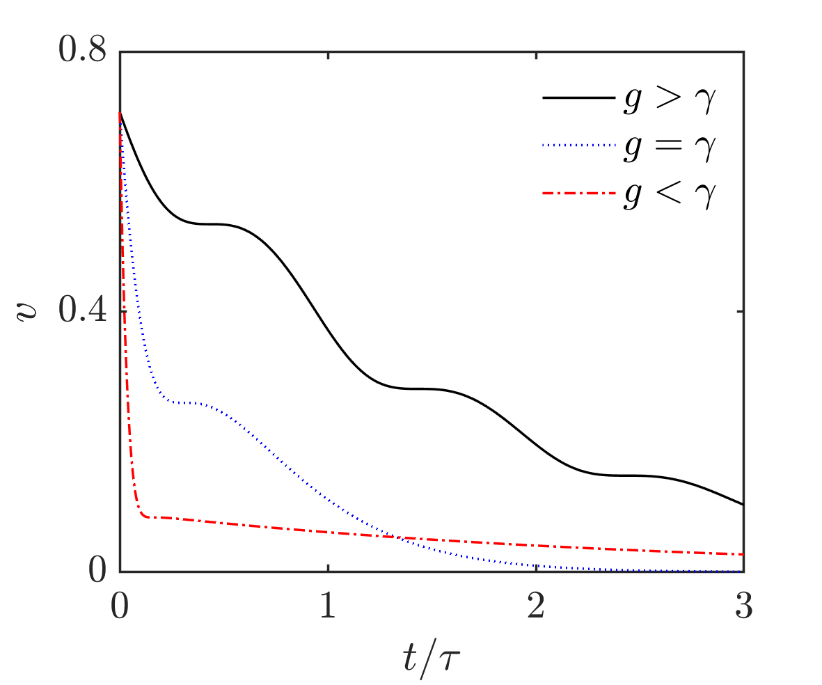
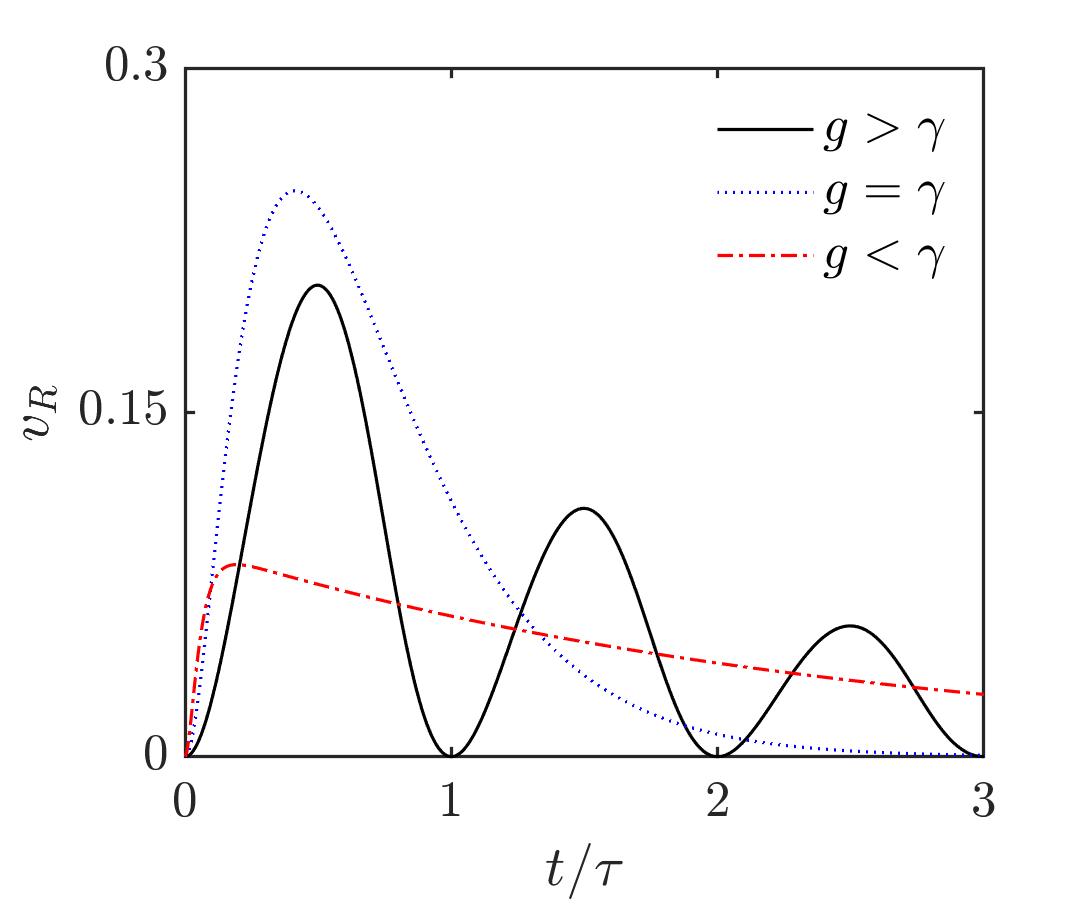
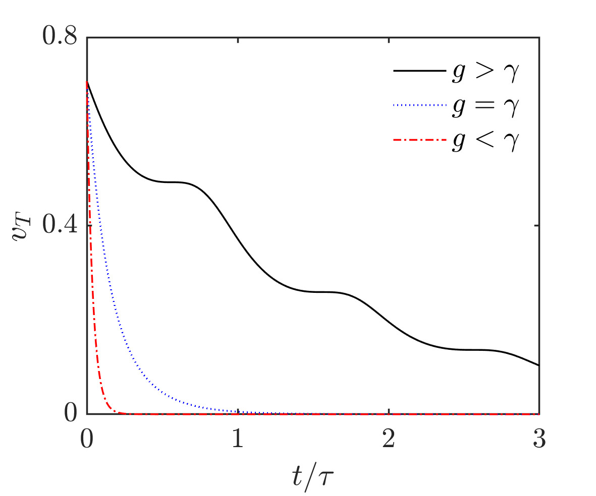
Figure 1: The behaviour of the evolution speed $v(t)$, its radial component $v_{R}(t)$, and its tangential component $v_{T}(t)$ are plotted here in the PT-symmetric model for which ${\hat{H}}=\frac{1}{2}g{\hat{\sigma}}_{x}$ and ${\hat{L}}=\sqrt{\gamma}{\hat{\sigma}}_{z}$. Each plot shows the speed as a function of time in three phases: the unbroken phase $g>\gamma$, the critical point $g=\gamma$, and the broken phase $g<\gamma$.

Acknowledgements. The author acknowledges support from the Russian Science Foundation, grant 20-11-20226, and is grateful to B. Longstaff for discussion.

References

References

- [1] Bender C M and Boettcher S 1998 Real spectra in non-Hermitian Hamiltonians having -symmetry Phys Rev Lett 80 5243–5246
- [2] Pontryagin L S 1944 Hermitian operators in spaces with indefinite metrics Bull Acad Sci URSS Ser Math [Izvestiya Akad Nauk SSSR] 8 243–280
- [3] Mostafazadeh A 2002 Pseudo-Hermiticity versus PT-symmetry III J Math Phys 43 3944–3951
- [4] Bender C M, Brody D C and Jones H F 2002 Complex extension of quantum mechanics Phys Rev Lett 89 27040
- [5] Mackey G W 1959 Commutative Banach Algebras (Rio De Janeiro: Instituto de Matematica pura e Aplicada do Conselho Nacional de Pesquisa)
- [6] Scholtz F G, Geyer H B and Hahne F J W 1992 Quasi-Hermitian operators in quantum mechanics and the variational principle Ann Phys 213 74–101
- [7] Mostafazadeh, A. 2003 Exact PT-symmetry Is equivalent to Hermiticity J Phys A36 7081–7091
- [8] Brody D C 2014 Biorthogonal quantum mechanics J Phys A47 035305
- [9] Brody D C 2016 Consistency of PT-symmetric quantum mechanics J Phys A49, 10LT03
- [10] Ruschhaupt A, Delgado F and Muga J G 2005 Physical realization of PT-symmetric potential scattering in a planar slab waveguide J Phys A38 L171–L176
- [11] Makris K G, El-Ganainy R, Christodoulides D N and Musslimani Z H 2008 Beam dynamics in PT-symmetric optical lattices Phys Rev Lett 100 103904
- [12] Klaiman S, Günther U and Moiseyev N 2008 Visualization of branch points in PT-symmetric waveguides Phys Rev Lett 101 080402
- [13] Kato T 1966 Perturbation Theory of Linear Operators (Berlin: Springer)
- [14] Berry M V 2004 Physics of nonhermitian degeneracies Czech J Phys 54 1039–1047
- [15] Heiss W D 2012 The physics of exceptional points J Phys A45 444016
- [16] Brody D C and Graefe E M 2013 Information geometry of complex Hamiltonians and exceptional points Entropy 15 3361–3378
- [17] Miri M. A. and Alu A 2019 Exceptional points in optics and photonics Science 363 eaar7709
- [18] Hatano N 2019 Exceptional points of the Lindblad operator of a two-level system Mol Phys 117 2121–2127
- [19] Minganti F, Miranowicz A, Chhajlany R W, and Nori F 2019 Quantum exceptional points of non-Hermitian Hamiltonians and Liouvillians: The effects of quantum jumps Phys Rev A100 062131
- [20] Brody D C and Longstaff B 2019 Evolution speed of open quantum dynamics Phys Rev Res 1 033127
- [21] Gorini V, Kossakowski A and Sudarshan E C G 1976 Completely positive dynamical symmetry groups of -level systems J Math Phys 17 821–825
- [22] Lindblad G 1976 On the generators of quantum dynamical semigroups. Commun Math Phys 48 119–130
- [23] Hawking S W 1982 The unpredictability of quantum gravity Commun Math Phys 87 395–415
- [24] Banks T, Susskind L and Peskin M 1984 Difficulties for the evolution of pure states into mixed states Nucl Phys B244 125–134
- [25] Dast D, Haag D, Cartarius H and Wunner G 2014 Quantum master equation with balanced gain and loss Phys Rev A90 052120
- [26] Dast D, Haag D, Cartarius H, Main J and Wunner G 2016 Bose-Einstein condensates with balanced gain and loss beyond mean-field theory Phys Rev A94 053601
- [27] Graefe E M, Korsch H J and Niederle A E 2008 Mean-field dynamics of a non-Hermitian Bose-Hubbard dimer Phys Rev Lett 101 150408
- [28] Brody D C and Hughston L P 1996 Geometry of quantum statistical inference Phys Rev Lett 77 2851–2854
- [29] Anandan J and Aharonov Y 1990 Geometry of quantum evolution Phys Rev Lett 65 1697–1700
- [30] Brody D C and Hughston L P 2001 Geometric quantum mechanics J Geo Phys 38 19–53
- [31] Luo S 2003 Wigner-Yanase skew information and uncertainty relations Phys Rev Lett 91 180403
- [32] Brody D C 2011 Information geometry of density matrices and state estimation. J Phy A44 252002
- [33] Campaioli F, Pollock F A, Binder F C and Modi K 2018 Tightening quantum speed limits for almost all states Phys Rev Lett 120 060409
- [34] Campaioli F, Pollock F A and Modi K 2019 Tight, robust, and feasible quantum speed limits for open dynamics Quantum 3 168
- [35] Mondal D and Pati A K 2016 Quantum speed limit for mixed states using an experimentally realizable metric Phys Lett A380 1395–1400
- [36] Deffner S and Campbell S 2017 Quantum speed limits: from Heisenberg’s uncertainty principle to optimal quantum control J Phys A50 453001
- [37] Alipour S, Mehboudi M and Rezakhani A T 2014 Quantum metrology in open systems: Dissipative Cramér-Rao bound Phy Rev Lett 112 120405
- [38] Funo K, Shiraishi N and Saito K 2019 Speed limit for open quantum systems New J Phys 21 013006
- [39] Uzdin R and Kosloff R 2016 Speed limits in Liouville space for open quantum systems Europhys Lett 115 40003
- [40] Deffner S and Lutz E 2013 Quantum speed limit for non-Markovian dynamics Phys Rev Lett 111 010402
- [41] Taddei M M, Escher B M, Davidovich L and de Matos Filho R L 2013 Quantum speed limit for physical processes Phys Rev Lett 110 050402
- [42] del Campo A, Egusquiza I L, Plenio M B and Huelga S F 2013 Quantum speed limit in open system dynamics Phys Rev Lett 110 050403
- [43] Brody D C 2013 Geometry of the complex extension of Wigner’s theorem J Phy A46 395301