A Stochastic Operator Framework for Optimization and Learning with Sub-Weibull Errors

Abstract

This paper proposes a framework to study the convergence of stochastic optimization and learning algorithms. The framework is modeled over the different challenges that these algorithms pose, such as (i) the presence of random additive errors (e.g. due to stochastic gradients), and (ii) random coordinate updates (e.g. due to asynchrony in distributed set-ups). The paper covers both convex and strongly convex problems, and it also analyzes online scenarios, involving changes in the data and costs. The paper relies on interpreting stochastic algorithms as the iterated application of stochastic operators, thus allowing us to use the powerful tools of operator theory. In particular, we consider operators characterized by additive errors with sub-Weibull distribution (which parameterize a broad class of errors by their tail probability), and random updates. In this framework we derive convergence results in mean and in high probability, by providing bounds to the distance of the current iteration from a solution of the optimization or learning problem. The contributions are discussed in light of federated learning applications.

I Introduction

Recent technological advances in a range of disciplines – from machine learning data-driven optimization control, with applications to smart power grids, traffic networks, healthcare, etc. – introduced a wide set of challenges to the implementation and analysis of optimization and learning algorithms. As a motivating example, we elaborate on these challenges in the context of federated learning [1, 2], which was designed to allow a set of agents to cooperatively train a model without the need to directly share data. Due to the distributed set-up, algorithms designed in this framework need to deal with asynchrony and limited or unreliable communications. This is similarly a challenge in any application where multi-agent systems are deployed, such as distributed optimization and parallel computing [3, 4, 5, 6]. Additionally, due to the size of available data-sets, the agents may need to resort to the use of stochastic gradients, which are computed on a sub-set of the available data [7, 8, 9]. This design choice then introduces inexactness in exchange for a lower computational burden. Alternatively, when gradients are not directly accessible, for example due to sparse users’ feedback [10], agents may need to approximate them from functional evaluations ($0$-th order gradients) [11, 12, 13]. Finally, the data on which the agents train their model may change over time, due to changes in the phenomenon being observed or new data arriving in real time [14, 15, 16, 17]. This turns the problem into an online learning problem, with the agents now tracking the optimal model as it changes in response to changes in the data.

Abstracting away from this example, in many applications of optimization and learning we need to design and analyze algorithms that are provably robust to different sources of stochasticity and changes in the data. In particular, in this paper we focus on the analysis side of this challenge by leveraging the formalism of operator theory. Operator theory has been shown to offer a valuable tool for the analysis of algorithms, both in traditional static settings [18, 19, 20, 21] and in online settings [14, 22, 16, 23]. The key insight is that algorithmic steps can be interpreted as operators (or maps when working in an Euclidean space), with fixed points of the operators coinciding with optimal solutions of the optimization or learning problem [20, 19, 21]. This link gives access to powerful tools to characterize the convergence of existing algorithms [20, 18, 21], and it further inspires the design of new ones, e.g. [24, 25, 26].

However, as discussed above, in many applications of interest the algorithms we need to analyze are stochastic, and hence are characterized by stochastic operators. In the following we discuss previous results in the analysis of stochastic operators. One source of stochasticity is that of random coordinate updates, in which only some part of the operator is applied at any given iteration [27, 28, 29, 4, 30, 6]. This class of operators model distributed algorithms in which only some agents, e.g. due to asynchrony, perform an update and hence apply the corresponding part of the algorithm/operator. Operators subject to additive errors, e.g. due to the use of stochastic gradients, have also been studied, see [29, 31, 27, 28, 7]. It is typical to handle stochastic errors in the algorithmic map or operator by either assuming that their norm vanishes asymptotically, or by multiplying them by a vanishing parameter. While this choice allows one to prove almost sure convergence, in many practical applications the additive error is not (or cannot be made) vanishing, especially in an online scenario.

To delineate our contribution in the context of the discussion above, we analyze algorithms that can be characterized by the stochastic iteration (formalized in section III):

$$x_{i}^{\ell+1}=\begin{cases}\mathcal{T}_{i}\mathbold{x}^{\ell}+e_{i}^{\ell}&\text{w.p.}\ p_{i}\\ x_{i}^{\ell}&\text{w.p.}\ 1-p_{i}\end{cases},\quad\ell\in\mathbb{N}$$ (1)

where $\mathcal{T}\mathbold{x}=(\mathcal{T}_{1}\mathbold{x},\ldots,\mathcal{T}_{n}\mathbold{x})$ is an operator, $\mathbold{x}=(x_{1},\ldots,x_{n})$, and $e_{i}^{\ell}$ is an additive error. The stochasticity in equation 1 has two sources: (i) each “coordinate” of the operator is updated with probability $p_{i}$ (e.g. due to asynchrony), and (ii) the update is performed using an inexact version of the operator (e.g. stochastic gradients). Additionally, we will be interested in the (iii) online scenario in which the operator changes over time to model applications in online optimization and learning; that is, at time $\ell+1$ we apply $\mathcal{T}_{i}^{\ell+1}$. The iteration equation 1 will be studied under the assumption that the operator is either contractive or averaged (in which case equation 1 can be seen as a stochastic Krasnosel’skiĭ-Mann).

As in e.g., [27, 28], we model inexact operators as operators subject to the additive errors $e_{i}$. However, differently from previous results, in this paper we perform our analysis for errors with sub-Weibull distributions. That is, the norm of $e_{i}$ satisfies

$$\mathbb{P}\left[\left\lVert e_{i}\right\rVert\geq\epsilon\right]\leq 2\exp\left(-\left(\frac{\epsilon}{\nu}\right)^{1/\theta}\right),\quad\forall\,\,\epsilon>0$$ (2)

for some parameters $\theta\geq 0$, $\nu>0$. The class of sub-Weibull r.v.s allows us to consider distributions for the additive errors that may have heavy tails [32, 33, 34, 35]; this class is also general and it includes the sub-Gaussian and sub-exponential classes as sub-cases, as well as random variable whose distribution has a finite support [36, 37]. As explained shortly, the sub-Weibull model will allow us to provide high probability bounds for the convergence of equation 1 by deriving pertinent concentration results. As defined in equation 2, sub-Weibull random variables are characterized by a tail parameter $\theta$, that defines the decay rate of the tails. Besides the convenient properties of the sub-Weibull class (e.g. closure under scaling, sum, and product) that allow for a unified theoretical analysis, there is growing evidence that high-tailed distributions arise in machine learning applications, see [32, 38, 39, 40].

Contributions. Overall, this paper offers the following contributions:

1. We study the convergence of equation 1, and provide convergence results in mean and in high probability when the errors follow a sub-Weibull distribution. In particular, bounds are offered for the distance from the fixed point (if the operator is contractive, i.e. the problem is strongly convex) or for the cumulative fixed point residual (if the operator is averaged, i.e. the problem is convex). These error bounds hold for any iteration $\ell\in\mathbb{N}$ with a given, arbitrary probability. We also show that the high-probability bounds – in the form $\mathbb{P}\left[\left\lVert x\right\rVert\leq\epsilon(\delta)\right]\geq 1-\delta$ for the random variable $x$ – scale with a factor $\sim\log(1/\delta)$, as opposed to a scaling $\sim 1/\delta$ that one would obtain via Markov’s inequality.

2. The framework we propose leverages a sub-Weibull model [32, 33, 34, 35] for the norm of the additive errors. To the best of our knowledge, this is the first time that sub-Weibull models are employed in combination with operator-theoretic tools. By using sub-Weibulls, we are able to model a very broad class of random variables, fitting different practical applications.

3. As mentioned above, the convergence results proposed in this paper hold with high probability, as opposed to the almost sure convergence results of e.g. [27]. We discuss the difference between the two viewpoints, and also further characterize the convergence of equation 1 in almost sure terms (under some additional assumptions, such as vanishing errors).

4. The analysis provided also holds in online scenarios, in which the operator characterizing equation 1 changes over time.

Organization. In section II we review some preliminaries in operator theory, and introduce the sub-Weibull formalism. In section III, building on the motivating example of federated learning, we formalize and discuss the stochastic framework. In sections IV and V we present and discuss, respectively, mean and high probability convergence results derived in the proposed framework. Finally, section VI presents some illustrative numerical results.

II Preliminaries

II-A Operators

Let $\mathbb{H}_{i}$, $i=1,\ldots,n$ be (possibly infinite-dimensional) Hilbert spaces with inner product $\langle\cdot,\cdot\rangle_{i}$, induced norm $\left\lVert\cdot\right\rVert_{i}$ and identity $\mathcal{I}_{i}:\mathbb{H}_{i}\to\mathbb{H}_{i}$. We consider the direct sum space $\mathbb{H}=\mathbb{H}_{1}\oplus\cdots\oplus\mathbb{H}_{n}$, whose elements are $\mathbold{x}=(x_{1},\ldots,x_{n})$ with $x_{i}\in\mathbb{H}_{i}$ for all $i=1,\ldots,n$. For $\mathbold{x},\mathbold{y}\in\mathbb{H}$, we define the inner product as $\langle\mathbold{x},\mathbold{y}\rangle=\sum_{i=1}^{n}\langle x_{i},y_{i}\rangle_{i}$, and denote the induced norm and identity of $\mathbb{H}$ as $\left\lVert\cdot\right\rVert$ and $\mathcal{I}:\mathbb{H}\to\mathbb{H}$, respectively. We consider operators $\mathcal{T}:\mathbb{H}\to\mathbb{H}$ defined as

$$\mathcal{T}\mathbold{x}=(\mathcal{T}_{1}\mathbold{x},\ldots,\mathcal{T}_{n}\mathbold{x})$$ (3)

where $\mathcal{T}_{i}:\mathbb{H}\to\mathbb{H}_{i}$ for all $i=1,\ldots,n$.

A central theme of the paper is to compute fixed points of a given operator via iterative algorithms. To this end, in the following we introduce pertinent definitions and results. For a background on operator theory we refer to e.g. [41, 20].

Definition 1 (Fixed points).

Let $\mathcal{T}:\mathbb{H}\to\mathbb{H}:\mathbold{x}\mapsto\mathcal{T}\mathbold{x}=(\mathcal{T}_{1}\mathbold{x},\ldots,\mathcal{T}_{n}\mathbold{x})$. The point $\bar{\mathbold{x}}\in\mathbb{H}$ is a fixed point of $\mathcal{T}$ if $\bar{\mathbold{x}}=\mathcal{T}\bar{\mathbold{x}}$. We denote the fixed set of $\mathcal{T}$ as $\operatorname{fix}(\mathcal{T})=\{\mathbold{x}\in\mathbb{H}\ |\mathbold{x}=\mathcal{T}\mathbold{x}\}$.

Notice that a fixed point $\bar{\mathbold{x}}=(\bar{x}_{1},\ldots,\bar{x}_{n})$ by definition is such that $\bar{x}_{i}=\mathcal{T}_{i}\bar{\mathbold{x}}$ for all $i=1,\ldots,n$. In the following, we review well-known definitions and properties of operators (see, e.g., [20]).

Definition 2 (Non-expansive, contractive).

The operator $\mathcal{T}$ is $\zeta$-Lipschitz continuous, $\zeta\geq 0$, if:

$$\left\lVert\mathcal{T}\mathbold{x}-\mathcal{T}\mathbold{y}\right\rVert\leq\zeta\left\lVert\mathbold{x}-\mathbold{y}\right\rVert,\quad\forall\mathbold{x},\mathbold{y}\in\mathbb{H}.$$ (4)

The operator is non-expansive if $\zeta=1$, and contractive if $\zeta\in(0,1)$.

Definition 3 (Averaged).

The operator $\mathcal{T}$ is averaged if and only if there exist $\alpha\in(0,1)$ and a non-expansive operator $\mathcal{R}:\mathbb{H}\to\mathbb{H}$ such that $\mathcal{T}=(1-\alpha)\mathcal{I}+\alpha\mathcal{R}$. Equivalently, $\mathcal{T}$ is $\alpha$-averaged if

$$\left\lVert\mathcal{T}\mathbold{x}-\mathcal{T}\mathbold{y}\right\rVert^{2}\leq\left\lVert\mathbold{x}-\mathbold{y}\right\rVert^{2}-\frac{1-\alpha}{\alpha}\left\lVert(\mathcal{I}-\mathcal{T})\mathbold{x}-(\mathcal{I}-\mathcal{T})\mathbold{y}\right\rVert^{2}$$

for any $\mathbold{x},\mathbold{y}\in\mathbb{H}$.

We discuss now the existence of fixed points of non-expansive operators operators.

Lemma 1 (Browder’s theorem).

Let $\mathbb{D}\subset\mathbb{H}$ be a non-empty, convex, compact subset, and let $\mathcal{T}:\mathbb{D}\to\mathbb{D}$ be non-expansive, then $\operatorname{fix}(\mathcal{T})\neq\emptyset$ [20, Theorem 4.29].

Lemma 2 (Banach-Picard theorem).

Let $\mathcal{T}:\mathbb{H}\to\mathbb{H}$ be a contractive operator, then $\operatorname{fix}(\mathcal{T})$ is a singleton [20, Theorem 1.50]. The unique fixed point is the limit of the sequence generated by:

$$\mathbold{x}^{\ell+1}=\mathcal{T}\mathbold{x}^{\ell},\quad\ell\in\mathbb{N}.$$

If we want to compute a fixed point of the non-expansive operator $\mathcal{T}$, the following results can be used.

Lemma 3.

Let $\mathcal{T}:\mathbb{H}\to\mathbb{H}$ be a non-expansive operator with $\operatorname{fix}(\mathcal{T})\neq\emptyset$. Then for any $\alpha\in(0,1)$, the $\alpha$-averaged operator $\mathcal{T}_{\alpha}=(1-\alpha)\mathcal{I}+\alpha\mathcal{T}$ is such that $\operatorname{fix}\left(\mathcal{T}_{\alpha}\right)=\operatorname{fix}(\mathcal{T})$.

Proof.

Let $\bar{\mathbold{x}}\in\operatorname{fix}(\mathcal{T})$, by definition $\bar{\mathbold{x}}=\mathcal{T}\bar{\mathbold{x}}$. Therefore given $\alpha\in(0,1)$ we have $(1-\alpha)\bar{\mathbold{x}}+\alpha\mathcal{T}\bar{\mathbold{x}}=\bar{\mathbold{x}}-\alpha\bar{\mathbold{x}}+\alpha\bar{\mathbold{x}}=\bar{\mathbold{x}}.$ ∎

Lemma 4 (Krasnosel’skiĭ-Mann theorem).

Let $\mathbb{D}\subset\mathbb{H}$ be a non-empty closed convex subset, and let $\mathcal{T}:\mathbb{D}\to\mathbb{D}$ be a non-expansive operator (notice that by Lemma 1 $\operatorname{fix}(\mathcal{T})\neq\emptyset$). Let $\alpha\in(0,1)$, then the Krasnosel’skiĭ-Mann iteration

$$\mathbold{x}^{\ell+1}=(1-\alpha)\mathbold{x}^{\ell}+\alpha\mathcal{T}\mathbold{x}^{\ell},\quad\ell\in\mathbb{N},$$

guarantees that $\left\lVert(\mathcal{I}-\mathcal{T})\mathbold{x}^{\ell}\right\rVert\to 0$ as $\ell\to\infty$ [20, Theorem 5.15].

In the remainder of the paper we will thus focus on studying the convergence of the Banach-Picard in two cases: i) when the operator is contractive, and ii) when it is averaged.

II-B Probability

In this section, we provide some definitions and results in probability theory that will be used in the paper to derive convergence results in high-probability. Throughout the paper, the underlying probability space will be $(\Omega,\mathcal{F},\mathbb{P})$. We start by introducing the definition of sub-Weibull random variables [35, 32, 33, 34].

Definition 4 (Sub-Weibull random variable).

A random variable $x$ is said to be sub-Weibull if there exist $\theta\geq 0$, $\nu>0$ such that

$$\left\lVert x\right\rVert_{k}=\mathbb{E}\left[|x|^{k}\right]^{1/k}\leq\nu k^{\theta},\quad\forall k\geq 1,$$

and we denote it by $x\sim\mathrm{subW}(\theta,\nu)$.

The following equivalence result relates the moments growth condition of Definition 4 with a bound for the tail probability [35, Lemma 5].

Lemma 5 (Sub-Weibull tail probability).

Let $x\sim\mathrm{subW}(\theta,\nu)$, then the tail probability verifies the bound

$$\mathbb{P}\left[|x|\geq\epsilon\right]\leq 2\exp\left(-\left(\frac{\epsilon}{c(\theta)\nu}\right)^{1/\theta}\right),\quad\forall\,\,\epsilon>0,$$ (5)

where $c(\theta):=(2e/\theta)^{\theta}$.

Lemma 5 shows that the tails of a sub-Weibull r.v. become heavier as the parameter $\theta$ grows larger. Moreover, setting $\theta=1/2$ and $\theta=1$ yields the class of sub-Gaussians and sub-exponential random variables, respectively; see, e.g., [36, 37]. The following lemma shows how the tail probability equation equation 5 can be used to give high probability bounds.

Lemma 6 (High probability bound).

Let $x\sim\mathrm{subW}(\theta,\nu)$, then for any $\delta\in(0,1)$, w.p. $1-\delta$ we have the bound:

$$|x|\leq\nu\log^{\theta}(2/\delta)c(\theta).$$

Proof.

By Lemma 5 we have, for any $\epsilon>0$:

$$\mathbb{P}\left[|x|\geq\epsilon\right]\leq 2\exp\left(-\left({\epsilon}/{(c(\theta)\nu)}\right)^{1/\theta}\right).$$

Setting the right-hand side equal to $\delta$ and solving for $\epsilon$ we get $\epsilon=c(\theta)\nu\log^{\theta}(2/\delta)$ which implies that, w.p. $1-\delta$ we have $|x|\leq\epsilon=c(\theta)\nu\log^{\theta}(2/\delta)$. ∎

We characterize now the properties of the sub-Weibull class of random variables.

Lemma 7 (Inclusion).

Let $x\sim\mathrm{subW}(\theta,\nu)$, then $x\sim\mathrm{subW}(\theta^{\prime},\nu^{\prime})$ for any $\theta^{\prime}\geq\theta$, $\nu^{\prime}\geq\nu$.

Proof.

By assumption we have $\left\lVert x\right\rVert_{k}\leq\nu k^{\theta}$. Using the fact that $\nu k^{\theta}\leq\nu^{\prime}k^{\theta^{\prime}}$ (which holds since $k\geq 1$) yields the thesis; cf. [32, Proposition 1]. ∎

Lemma 8 (Closure).

The class of sub-Weibull random variables is closed w.r.t. product by a scalar, sum, product, and exponentiation, according to the following rules.

1. Product by scalar: let $x\sim\mathrm{subW}(\theta,\nu)$ and $a\in\mathbb{R}$, then $ax\sim\mathrm{subW}(\theta,|a|\nu)$;

2. Sum: let $x_{i}\sim\mathrm{subW}(\theta_{i},\nu_{i})$, $i=1,2$, possibly dependent, then $x_{1}+x_{2}\sim\mathrm{subW}(\max\{\theta_{1},\theta_{2}\},\nu_{1}+\nu_{2})$;

3. Product: let $x_{i}\sim\mathrm{subW}(\theta_{i},\nu_{i})$, $i=1,2$, and independent, then $x_{1}x_{2}\sim\mathrm{subW}(\theta_{1}+\theta_{2},\nu_{1}\nu_{2})$.

4. Power: let $x\sim\mathrm{subW}(\theta,\nu)$ and $a>0$, then $x^{a}\sim\mathrm{subW}(a\theta,\nu^{a}\max\{1,a^{a\theta}\})$.

Proof.

See appendix A. ∎

We conclude with some remarks.

Remark 1 (Square of sub-Weibull).

A consequence of 4) in Lemma 8 is that the square of $x\sim\mathrm{subW}(\theta,\nu)$ is itself a sub-Weibull, characterized by $x^{2}\sim\mathrm{subW}(2\theta,4^{\theta}\nu^{2})$. A particular case is the well known fact that the square of a sub-Gaussian ($\theta=1/2$) is sub-exponential ($\theta=1$), see e.g. [37, Lemma 2.7.6].

Remark 2 (Mean of sub-Weibulls).

Notice that the definition of sub-Weibulls and their properties does not require that their mean be zero. Moreover, if $x\sim\mathrm{subW}(\theta,\nu)$ and $x\geq 0$ almost surely, then $\mathbb{E}\left[x\right]\leq\nu$, since $\left\lVert x\right\rVert_{1}=\mathbb{E}\left[x\right]$.

Remark 3 (Bounded r.v.s).

We can see that bounded r.v.s are sub-Weibull with $\theta=0$; indeed, let $x$ be a r.v. such that a.s. $|x|\leq b$, then $\left\lVert x\right\rVert_{k}\leq b=bk^{0}$, $k\geq 1$. This characterization is “optimal” in terms of $\theta$, since $\theta=0$ corresponds to the lightest possible tail. However, it is sub-optimal in the other parameter, $\nu$, which does not reflect the overall distribution of $x$, only its maximum absolute value. Alternatively, we know by [37, p. 24] that the class of sub-Gaussian random variables includes that of bounded r.v.s; this implies that bounded r.v.s are sub-Weibull with $\theta=1/2$.

III Motivation and Framework Development

We start this section by discussing a motivating example in the context of federated learning [1, 2], around which we will formalize our stochastic operator framework.

III-A Motivating example: federated learning

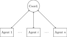
Figure 1: The architecture in federated learning.

In federated learning, a set of $n$ agents, aided by a coordinator, aim to cooperatively train a model without directly sharing the data they store [1, 2]. In order to keep the data private, the agents share the results of local training with the coordinator, which aggregates them into a more accurate model. Formally, the goal is to solve the optimization problem

$$\min_{x_{i}\in\mathbb{R}^{p}}\sum_{i=1}^{n}f_{i}(x_{i})\quad\text{s.t.}\ x_{1}=x_{2}=\ldots=x_{n}$$ (6)

where $f_{i}:\mathbb{R}^{p}\to\mathbb{R}\cup\{+\infty\}$ is the loss function of agent $i$, defined over the local dataset. Let $\{d_{i}^{h}\}_{h=1}^{m_{i}}$ be the $m_{i}$ data points stored by $i$, then usually the local loss is of the form

$$f_{i}(x)=\sum_{h=1}^{m_{i}}\lambda(x;d_{i}^{h})$$ (7)

with $\lambda$ being a training loss (e.g. quadratic or logistic).

In principle, equation 6 could be solved via gradient descent by applying

$$x^{\ell+1}=\mathcal{T}x^{\ell}:=\frac{1}{n}\sum_{i=1}^{n}\left(x^{\ell}-\gamma\nabla f_{i}(x^{\ell})\right),\quad\ell\in\mathbb{N},$$ (8)

where the agents compute local gradient descent steps and the coordinator averages them. However, when solving learning problems there are several practical constraints that make implementing equation 8 unrealistic. In the following we discuss some of these practical challenges, and how they motivate the theoretical developments of subsequent sections. The section concludes by presenting a modified version of equation 8 that accounts for these challenges, and which can be interpreted as a stochastic operator, fitting in the framework of section III-B.

Challenge 1: additive errors

Learning problems are often high dimensional, both in the size of the unknown $x\in\mathbb{R}^{p}$ (especially when training neural networks), and in the size of the local data sets. The size of the unknown poses a first challenge, since algorithm equation 8 requires sharing of $p$-dimensional vectors, and the larger $p$ the more expensive these communications become. In practice, then, quantization or compression is applied before the agents communicate with the coordinator [42], lessening the burden at the cost of introducing some error.

A second challenge arises when computing the gradient of local losses equation 7, since the larger $m_{i}$ is the more computationally expensive gradient computations are. To reduce the cost of gradient evaluations, a standard strategy in learning is to use stochastic gradients [43], which approximate the true gradient using only a random subset of the local data points. But, similarly to communications reduction techniques, approximating local gradients introduces some error.

We are therefore interested in analyzing the modified version of equation 8 given by $x^{\ell+1}=\mathcal{T}x^{\ell}+e^{\ell},$ where $e^{\ell}$ is a random vector modeling the errors introduced by the use of inexact communications and stochastic gradients.

Challenge 2: asynchrony

The agents cooperating in the learning procedure may be highly heterogeneous, in that they have different computational resources [2]. In equation 8 all the agents compute a local gradient at the same time – however, heterogeneous agents will have different computation times. Therefore, requiring the agents to work synchronously implies that the faster agents will sit idle while waiting for the slower ones to conclude the local computations [3].

One way to solve this problem is to allow asynchronous activation of the agents, so that each agent is free to perform local training at its own pace. More formally, let $\mathbb{I}^{\ell}\subset\{1,\ldots,n\}$, $|\mathbb{I}^{\ell}|\leq n$, be the subset of agents that concluded a local computation at time $\ell\in\mathbb{N}$. Then we are interested in algorithms in which the coordinator only aggregates information from $\mathbb{I}^{\ell}$, instead of all agents. Algorithm 1 presents a modified version of equation 8 that allows for asynchronous activations (see appendix B for the derivation).

We also remark that asynchrony could be enforced by design as an additional measure to reduce the amount of communications required at each time.

Challenge 3: online problems

The problem equation 6 discussed so far is static, in the sense that the data sets defining the local losses do not change over time. However, in many learning applications the agents may be continuously collecting new data and consequently modifying their loss. This results in an online learning problem, characterized by [14, 15, 16]

$$\min_{x_{i}\in\mathbb{R}^{p}}\sum_{i=1}^{n}f_{i}^{\ell}(x_{i})\quad\text{s.t.}\ x_{1}=x_{2}=\ldots=x_{n}.$$

In this set-up the solution(s) to the problem at time $\ell\in\mathbb{N}$ may not coincide with those at time $\ell+1$, and our analysis of Algorithm 1’s performance needs to account for this fact.

Algorithm 1 Federated gradient descent.

1:Initial conditions $z^{0}$, $x_{i}^{0}$, and step-size $\gamma$.

2:for $\ell=0,1,2,\ldots$ 

3:     // compressed communications

4:     the coordinator transmits $z^{\ell}$ to the active agents $\mathbb{I}^{\ell}$

5:     for $i\in\{1,\ldots,n\}$ 

6:         // asynchrony

7:         if $i\in\mathbb{I}^{\ell}$ then

8:              // inexact gradients

9:              the agent performs a local gradient step

$$x_{i}^{\ell+1}=z^{\ell}-\gamma\nabla f_{i}(z^{\ell})$$

10:              // compressed communications

11:              and transmits $x_{i}^{\ell+1}$ to the coordinator

12:         else

13:              otherwise sets $x_{i}^{\ell+1}=x_{i}^{\ell}$

14:         end if

15:     end for

16:     the coordinator computes

$$z^{\ell+1}=\frac{1}{n}\left(\sum_{i\in\mathbb{I}^{\ell}}x_{i}^{\ell+1}+\sum_{i\not\in\mathbb{I}^{\ell}}x_{i}^{\ell}\right)$$

17:end for

III-B Stochastic operator framework

Motivated by the example discussed so far, we are now ready to formalize the stochastic operator framework of interest in this paper. Consider an operator $\mathcal{T}\mathbold{x}=(\mathcal{T}_{1}\mathbold{x},\ldots,\mathcal{T}_{n}\mathbold{x})$, in the following we analyze the convergence of the update, for $i=1,\ldots,n$:

$$x_{i}^{\ell+1} =\begin{cases}\mathcal{T}_{i}^{\ell+1}\mathbold{x}^{\ell}+e_{i}^{\ell}&\text{w.p.}\ p_{i}\\ x_{i}^{\ell}&\text{w.p.}\ 1-p_{i}\end{cases}$$ (9)

$$=(1-u_{i}^{\ell})x_{i}^{\ell}+u_{i}^{\ell}\left(\mathcal{T}_{i}^{\ell+1}\mathbold{x}^{\ell}+e_{i}^{\ell}\right)$$

$$=:\hat{\mathcal{T}}_{i}^{\ell+1}\mathbold{x}^{\ell}+u_{i}^{\ell}e_{i}^{\ell}$$

where $\ell\in\mathbb{N}$ is the iteration index, $u_{i}^{\ell}$ are Bernoulli random variables that indicate whether a coordinate is updated or not at iteration $\ell$, and $\mathbold{e}^{\ell}=(e_{1}^{\ell},\ldots,e_{n}^{\ell})$ is a random vector of additive noise. As discussed in section III-A, in federated learning only the coordinates corresponding to active nodes (with $u_{i}^{\ell}$) are updated, and additive noise may be due to inexact communications or stochastic gradients (hence $e_{i}^{\ell}$). The operator $\mathcal{T}^{\ell}$ is allowed to change over time to account for online learning problems defined by streaming sources of data.

In the following we introduce and discuss some assumptions to formalize the framework. We remark that throughout the paper, the initial condition $\mathbold{x}^{0}\in\mathbb{H}$ will be assumed to be deterministic.

Assumption 1 (Stochastic framework).

The following is assumed.

• $\mathbold{u}^{\ell}=(u_{1}^{\ell},\ldots,u_{n}^{\ell})$ is a $\{0,1\}^{n}$-valued random vector with $p_{i}:=\mathbb{P}\left[u_{i}=1\right]>0$, $i=1,\ldots,n$.

• The additive error $\mathbold{e}^{\ell}\in\mathbb{H}$ is an $\mathbb{H}$-valued random vector such that its norm is sub-Weibull, that is $\left\lVert\mathbold{e}^{\ell}\right\rVert\sim\mathrm{subW}(\theta,\nu)$.

• The random processes $\{\mathbold{u}^{\ell}\}_{\ell\in\mathbb{N}}$ and $\{\mathbold{e}^{\ell}\}_{\ell\in\mathbb{N}}$ are i.i.d. and independent of each other.

We provide now two assumptions on the operator defining (9), which will be used to provide two different sets of results. Notice that these assumptions apply to the underlying deterministic operator $\mathcal{T}^{\ell+1}$ only.

Assumption 2 (Contractive operator).

Consider an operator $\mathcal{T}^{\ell}:\mathbb{D}\to\mathbb{D}$. The following is assumed.

• The operator $\mathcal{T}^{\ell}:\mathbb{H}\to\mathbb{H}$ is $\zeta$-contractive for all $\ell\in\mathbb{N}$, and we denote by $\bar{\mathbold{x}}^{\ell}$ its unique fixed point.

• There exists $\sigma\geq 0$ such that the fixed points of consecutive operators have a bounded distance

  $$\left\lVert\bar{\mathbold{x}}^{\ell}-\bar{\mathbold{x}}^{\ell-1}\right\rVert\leq\sigma,\quad\forall\ell\in\mathbb{N}.$$

Assumption 3 (Averaged operator).

Consider an operator $\mathcal{T}^{\ell}:\mathbb{D}\to\mathbb{D}$. the following is assumed.

• The operator $\mathcal{T}^{\ell}:\mathbb{D}\to\mathbb{D}$ is $\alpha$-averaged for all $\ell\in\mathbb{N}$, with $\mathbb{D}\subset\mathbb{H}$ being convex and compact. In the following we denote by $\operatorname{diam}(\mathbb{D})$ the diameter of $\mathbb{D}$.

• There exists $\sigma\geq 0$ such that given $\bar{\mathbold{x}}^{\ell}\in\operatorname{fix}(\mathcal{T}^{\ell})$, $\ell\in\mathbb{N}$, then

  $$\inf_{\bar{\mathbold{x}}^{\ell-1}\in\operatorname{fix}(\mathcal{T}^{\ell-1})}\left\lVert\bar{\mathbold{x}}^{\ell}-\bar{\mathbold{x}}^{\ell-1}\right\rVert\leq\sigma.$$

Before moving on to the convergence analysis, we discuss the framework and the assumptions that characterize it.

III-B1 Update model

We note that Assumption 1(i) does not require independence among the components of $\mathbold{u}^{\ell}$. Independence is only assumed between $\mathbold{u}^{\ell}$ and $\mathbold{u}^{h}$, for any pair $\ell,h\in\mathbb{N}$, $\ell\neq h$.

Under Assumption 1(i) there may exist times during which none of the coordinates are updated, because $u_{i}^{\ell}=0$ for all $i=1,\ldots,n$. This is different from the framework used in e.g. [27, 28], where at least one $u_{i}^{\ell}$ must always be different from zero. Accounting for such events is important in online scenarios, where the problem changes (e.g. due to changes in the environment) even when updates are not performed.

III-B2 Additive error model

The additive error model defined in Assumption 1(ii) is very general, since it imposes only a tail condition on the error norm. For example, stochastic gradients have been shown to exhibit heavy tails in learning [39, 40]. Moreover, by Remark 3 bounded errors (such as quantization errors) are also sub-Weibull in norm. The model we use for the additive errors implies that they are persistently present over time. This sets the paper apart from previous works on stochastic operators in which the additive error is assumed to decay to zero (or, equivalently, that the error is multiplied by a decaying parameter) [27, 28, 29].

We remark that Assumption 1 does not require independence of the error components at a fixed time $\ell$, or between the errors drawn at different times $\ell$ and $h$. Finally, the errors could also be biased, that is, they could have mean different from zero (either positive or negative). The sub-Weibull model that we use indeed allows for biased r.v.s, see e.g. the discussion in [32].

III-B3 Operators

In Assumption 3, the operators are defined on a compact $\mathbb{D}$, which is verified when for example $\mathcal{T}^{\ell}$ contain a projection onto $\mathbb{D}$. On the one hand, this implies that Browder’s theorem (cf. Lemma 1) holds, and hence that the operators have a non-empty fixed set. On the other, it allows us to guarantee that additive errors do not lead to divergence. This assumption is not required in e.g. [27] since the additive errors converge to zero asymptotically, and thus cannot lead to divergence.

In the context of convex optimization, we can relate Assumptions 2 and 3 to the properties of the cost function on which the operator $\mathcal{T}^{\ell}$ is defined. For example, in the federated learning set-up of section III-A convex loss functions yield averaged operators, while strongly convex ones yield contractive operators [21] (cf. also the discussion in appendix B).

Finally, a remark about the dynamic nature of the operators. As discussed in section III-A, in many applications we may be interested in solving optimization problems that change over time, as new data come in [44, 16], which motivates our choice to analyze time-varying operators. In this context, we can interpret equation 9 as an online algorithm, in which the output ($\mathbold{x}^{\ell}$) computed at time $\ell$ is used to warm-start the computation at time $\ell+1$. For this reason, it is necessary to provide bounds on the difference between consecutive operators (or equivalently, consecutive problems) to ensure that they are “close enough” for the warm-starting to provide an improvement in performance. This guarantee is provided by Assumption 2(ii) and Assumption 3(ii), which can be obtained for example bounding the rate of change of the operators.

IV Mean Convergence Analysis

We start by characterizing in section IV-A the mean convergence of equation 9 for contractive and averaged operators. The results and their implications will be discussed in section IV-B, while section IV-C will present some corollaries on the asymptotic convergence.

IV-A Main results

Proposition 1 (Mean – contractive operators).

Let Assumptions 1 and 2 hold, and let $\{\mathbold{x}^{\ell}\}_{\ell\in\mathbb{N}}$ be the sequence generated by equation 9. Then we have the following bound, for any $\ell\in\mathbb{N}$

$$\mathbb{E}\left[\left\lVert\mathbold{x}^{\ell}-\bar{\mathbold{x}}^{\ell}\right\rVert\right]\leq\sqrt{\frac{\bar{p}}{\underaccent{\bar}{p}}}\left(\chi^{\ell}\left\lVert\mathbold{x}^{0}-\bar{\mathbold{x}}^{0}\right\rVert+\frac{1-\chi^{\ell}}{1-\chi}(\chi\sigma+\nu)\right)$$

where $\bar{p}:=\max_{i}p_{i}$, $\underaccent{\bar}{p}:=\min_{i}p_{i}$, and $\chi:=\sqrt{1-\underaccent{\bar}{p}+\underaccent{\bar}{p}\zeta^{2}}\in(0,1).$

Proof.

See section C-A. ∎

Proposition 2 (Mean – averaged operators).

Let Assumptions 1 and 3 hold, and let $\{\mathbold{x}^{\ell}\}_{\ell\in\mathbb{N}}$ be the sequence generated by equation 9. Then we have the following bound, for any $\ell\in\mathbb{N}$

$$\mathbb{E}\left[\frac{1}{\ell+1}\sum_{h=0}^{\ell}\left\lVert(\mathcal{I}-\mathcal{T}^{h})\mathbold{x}^{h}\right\rVert^{2}\right]\leq\frac{\alpha}{\underaccent{\bar}{p}(1-\alpha)}\times$$

$$\times\left(\frac{1}{\ell+1}\left\lVert\mathbold{x}^{0}-\bar{\mathbold{x}}^{0}\right\rVert^{2}+\sigma^{2}+4^{\theta}\nu^{2}+2\operatorname{diam}(\mathbb{D})(\sigma+\nu)\right)$$

Proof.

See section C-B. ∎

IV-B Discussion

IV-B1 Difference from deterministic convergence

In the following we discuss the difference between Propositions 1 and 2 and the convergence of the static and deterministic update $\mathbold{x}^{\ell+1}=\mathcal{T}\mathbold{x}^{\ell}$, $\ell\in\mathbb{N}$.

Contractive case

By contractiveness we know that $\mathbold{x}^{\ell+1}=\mathcal{T}\mathbold{x}^{\ell}$ converges linearly to $\operatorname{fix}(\mathcal{T})=\{\bar{\mathbold{x}}\}$, that is $\left\lVert\mathbold{x}^{\ell}-\bar{\mathbold{x}}\right\rVert\leq\zeta^{\ell}\left\lVert\mathbold{x}^{0}-\bar{\mathbold{x}}\right\rVert$ [20, Theorem 1.50]. Comparing this bound with that of Proposition 1 we notice first of all that the introduction of random coordinate updates degrades the convergence rate – in mean – from $\zeta$ to $\chi\geq\zeta$, in accordance with the results of [28].

Secondly, the presence of additive errors implies that we do not reach exact convergence to the fixed point, but rather to a neighborhood thereof. Moreover, at any given time $\ell\in\mathbb{N}$, the additive error may cause the overall stochastic operator to be expansive $\left\lVert\mathbold{x}^{\ell+1}-\bar{\mathbold{x}}\right\rVert\geq\left\lVert\mathbold{x}^{\ell}-\bar{\mathbold{x}}\right\rVert$, but the underlying contractiveness of $\mathcal{T}$ ensure that this lead to inexact convergence rather than divergence.

Averaged case

The convergence of equation 9 for averaged operators can be proved only in terms of the cumulative fixed point residual $\frac{1}{\ell+1}\sum_{h=0}^{\ell}\left\lVert(\mathcal{I}-\mathcal{T}^{h})\mathbold{x}^{h}\right\rVert^{2}$, due to averagedness being weaker than contractiveness. On the other hand, for the deterministic update $\mathbold{x}^{\ell+1}=\mathcal{T}\mathbold{x}^{\ell}$ it is possible to prove that $\{\left\lVert(\mathcal{I}-\mathcal{T})\mathbold{x}^{\ell}\right\rVert\}_{\ell\in\mathbb{N}}$ is a monotonically decreasing sequence that converges to zero [20, Theorem 5.15]. Similarly to the contractive case, this is no longer the case in the presence of additive errors, and the metric used to analyze convergence needs to account for the overall evolution of the fixed point residual.

We remark that the concept of cumulative fixed point residual is similar to that of regret in convex optimization, and in particular to that of dynamic regret in online optimization [45]. Moreover, it includes as a particular case the different concept of regret based on the residual of the proximal gradient method proposed in [46].

IV-B2 Time-variability

As mentioned in section III-A, the stochastic framework we analyze allows for the operator to change over time, as this models online optimization algorithms [44, 16]. But the time-variability of the operators, and hence of their fixed point(s), can be seen as a second source of additive errors besides $\mathbold{e}^{\ell}$. This error is always present, also when no update is performed, to account for the fact that the environment changes at every iteration $\ell\in\mathbb{N}$. This is the case in online optimization when the problem depends on e.g. measurements of a system, and the system will evolve even when no measurement is performed.

Path length

In online optimization, a widely used concept is that of path-length, that is, the cumulative distance between consecutive optimizers. This concept can be straightforwardly extended to the operator theoretical set-up, by defining it as the cumulative distance between consecutive fixed points: $\sum_{h=0}^{\ell-1}\left\lVert\bar{\mathbold{x}}^{h+1}-\bar{\mathbold{x}}^{h}\right\rVert\leq\ell\sigma.$ The path-length often appears in regret bounds, see e.g. [45], but notice that in the worst case it grows linearly with $\ell$, and to carry out the convergence analysis the additional assumption that it grows sub-linearly is required. What instead appears in our bound is a weighted path-length

$$\sum_{h=0}^{\ell-1}\chi^{\ell-h-1}\left\lVert\bar{\mathbold{x}}^{h+1}-\bar{\mathbold{x}}^{h}\right\rVert\leq\frac{1-\chi^{\ell}}{1-\chi}\sigma$$

which asymptotically reaches a fixed value, independent of $\ell$. This is due to the fact that we use the contractiveness of the operator, allowing to reach a tighter bound.

IV-B3 Convergence without random coordinate updates

We remark that the results of Propositions 1 and 2 can be adapted in a straightforward manner to a scenario where no random coordinate updates are performed. Indeed, if $p_{i}=1$, $i=1,\ldots,n$ then the two results provide bounds to the convergence of inexact operators modeled by

$$\mathbold{x}^{\ell+1}=\mathcal{T}\mathbold{x}^{\ell}+\mathbold{e}^{\ell},\quad\ell\in\mathbb{N}.$$

This class of stochastic updates includes several optimization methods such as stochastic gradient descent and $0$-th order methods [7, 8, 9, 11, 12, 13], which are widely used in machine learning applications.

Section V-C will instead provide some convergence results when only random coordinate updates are present.

IV-C Asymptotic convergence results

The mean convergence results of section IV-A can be further used to characterize the asymptotic, almost sure convergence of (9), as proved in the following. The results are presented in the contractive case (cf. Assumption 2), but the same argument can be applied in the averaged case as well.

IV-C1 Convergence to a neighborhood

We start by showing that the output of equation 9 asymptotically and almost surely converges to a bounded neighborhood of the fixed point trajectory $\{\bar{\mathbold{x}}^{\ell}\}_{\ell\in\mathbb{N}}$.

Corollary 1 (Asymptotic a.s. convergence to neighborhood).

Let Assumptions 1 and 2 hold, and let $\{\mathbold{x}^{\ell}\}_{\ell\in\mathbb{N}}$ be the sequence generated by equation 9. Then for each coordinate, $i=1,\ldots,n$ it holds that:

$$\limsup_{\ell\to\infty}\left\lVert\mathbold{x}^{\ell}-\bar{\mathbold{x}}^{\ell}\right\rVert\leq\sqrt{\frac{\bar{p}}{\underaccent{\bar}{p}}}\frac{\chi\sigma+\nu}{1-\chi}\qquad\text{a.s.}.$$

Proof.

See section C-C. ∎

IV-C2 Exact asymptotic convergence

Corollary 1 shows that in general we can only prove asymptotic convergence to a neighborhood of the fixed point trajectory. The following result proves that zero asymptotic error can be achieved under the assumptions that the additive error $\mathbold{e}^{\ell}$ and the rate of the change of the operators $\mathcal{T}^{\ell}$ are vanishing.

Corollary 2 (Exact a.s. convergence).

Let Assumptions 1 and 2 hold, with the difference that

• the errors are vanishing, with $\mathbold{e}^{\ell}\sim\mathrm{subW}(\theta,\nu^{\ell})$ and $\lim_{\ell\to\infty}\nu^{\ell}=0$;

• for all $\ell\in\mathbb{N}$, $\mathcal{T}^{\ell}=\mathcal{T}$; we denote by $\bar{\mathbold{x}}$ the unique fixed point of $\mathcal{T}$.

Let $\{\mathbold{x}^{\ell}\}_{\ell\in\mathbb{N}}$ be the sequence generated by equation 9, then

$$\limsup_{\ell\to\infty}\left\lVert\mathbold{x}^{\ell}-\bar{\mathbold{x}}\right\rVert=0\qquad\text{a.s.}.$$

Proof.

See section C-D. ∎

The result of Corollary 2 is similar to [27, 28], in which the additive errors are assumed to be vanishing (or to be multiplied by a vanishing parameter).

Corollaries 1 and 2 leveraged Markov’s inequality to characterize the almost sure behavior of equation 9 – but these results hold only asymptotically, and do not characterize the transient. The question then is: can we provide high probability bounds that hold for any $\ell\in\mathbb{N}$? A first observation is that almost sure convergence cannot be guaranteed during the transient, owing to the ever-present disturbance of the additive errors $\mathbold{e}^{\ell}$. The next section will instead provide transient bounds that hold with assigned probability.

V High Probability Convergence Analysis

V-A Main results

The results of this section are derived applying the concept of sub-Weibull random variables (cf. section II-B), to equation 9. In addition to the assumptions on equation 9 discussed in section III-B, we also introduce the following.

Assumption 4 (Almost sure non-expansiveness).

The random coordinate update operators $\hat{\mathcal{T}}^{\ell}$ defined in equation 9 are such that, for all $\ell\in\mathbb{N}$, $\mathbold{x}\in\mathbb{H}$, and $\bar{\mathbold{x}}^{\ell}\in\operatorname{fix}(\mathcal{T}^{\ell})$:

$$\left\lVert\hat{\mathcal{T}}^{\ell}\mathbold{x}-\bar{\mathbold{x}}^{\ell}\right\rVert\leq\left\lVert\mathbold{x}-\bar{\mathbold{x}}^{\ell}\right\rVert\qquad\text{a.s.}.$$

This assumption implies that the stochastic operators $\hat{\mathcal{T}}^{\ell}$ are almost surely quasi-nonexpansive [20, Definition 4.1], that is, they are non-expansive w.r.t. any fixed point ($\mathbold{y}\in\mathbb{H}$ in Definition 2 is replaced by a fixed point). This is similar to the assumption in stochastic gradient descent (SGD) that the approximate gradient being used is a direction of sufficient descent, or that, in other words, the angle between true and approximate gradient is sufficiently positive [9, p. 243 and Assumption 4.3(b)].

Proposition 3 (High prob. – contractive operators).

Let Assumptions 1, 2 and 4 hold, and let $\{\mathbold{x}^{\ell}\}_{\ell\in\mathbb{N}}$ be the sequence generated by equation 9. Then for any $\ell\in\mathbb{N}$, given $\delta\in(0,1)$, with probability $1-\delta$ the following bound holds:

$$\left\lVert\mathbold{x}^{\ell}-\bar{\mathbold{x}}^{\ell}\right\rVert\leq\log^{\theta^{\prime}}(2/\delta)c(\theta^{\prime})\times$$

$$\qquad\times\Big{(}\eta(\ell)\left\lVert\mathbold{x}^{0}-\bar{\mathbold{x}}^{0}\right\rVert+\frac{1-\zeta^{\ell}}{1-\zeta}\frac{\sigma}{p}+\nu\sum_{h=0}^{\ell}\eta(\ell-h-1)\Big{)}$$

where $\theta^{\prime}=\max\{1,\theta\}$, $p=\prod_{i=1}^{n}p_{i}$, and $\eta(\ell)$ is defined in Lemma 9 and is such that $\eta(\ell)\in[0,1)$ and $\lim_{\ell\to\infty}\eta(\ell)=0$.

Proof.

See section D-A. ∎

Lemma 9.

Let $\beta(\ell)\sim\mathcal{B}(p,\ell)$, $\ell\in\mathbb{N}$, and $\zeta\in(0,1)$. Then we have $\zeta^{\beta(\ell)}\sim\mathrm{subW}(1/2,\eta(\ell))$ with $\eta(\ell)\in[0,1)$ defined by

$$\eta(\ell):=\max_{k}\left(1-p+p\zeta^{k}\right)^{\ell/k}/\sqrt{k}.$$ (10)

Proof.

See section D-B. ∎

We can see from equation 10 that $\eta(\ell)$ is a decreasing function of $\ell$, and that it takes values in $[0,1)$, where $0$ is attained when $k\to\infty$. Notice that $\eta(\ell)<1$ since the numerator is $<1$ even if $k=1$.

We turn now to the convergence analysis for averaged operators.

Proposition 4 (High prob. – averaged operators).

Let Assumptions 1, 3 and 4 hold, and let $\{\mathbold{x}^{\ell}\}_{\ell\in\mathbb{N}}$ be the sequence generated by equation 9. Then for any $\ell\in\mathbb{N}$, given $\delta\in(0,1)$, with probability $1-\delta$ the following bound holds:

$$\frac{1}{\ell+1}\sum_{h=0}^{\ell}u^{h}\left\lVert(\mathcal{I}-\mathcal{T}^{h})\mathbold{x}^{h}\right\rVert^{2}\leq\log^{2\theta}(2/\delta)c(2\theta)\times$$

$$\times\frac{\alpha}{1-\alpha}\left(\frac{\left\lVert\mathbold{x}^{0}-\bar{\mathbold{x}}^{0}\right\rVert^{2}}{\ell+1}+\sigma^{2}+4^{\theta}\nu^{2}+2\operatorname{diam}(\mathbb{D})(\sigma+\nu)\right),$$

where $u^{h}\sim Ber(p)$, with $p=\prod_{i=1}^{n}p_{i}$.

Proof.

See section D-C. ∎

V-B Discussion

V-B1 Assumption 4

In section IV we were able to provide a mean convergence analysis under the standard assumptions of either contractiveness or averagedness. This is possible because in mean the operator $\hat{\mathcal{T}}^{\ell}$ preserves its properties. For example if $\mathcal{T}^{\ell}$ is $\zeta$-contractive, then so is $\hat{\mathcal{T}}^{\ell}$ in mean, albeit with a larger constant. However, when analyzing the convergence in high probability we can no longer rely on the mean contractiveness – indeed, for some particular realizations of $\mathbold{u}^{\ell}$ the operator $\hat{\mathcal{T}}^{\ell}$ may be expansive. Introducing Assumption 4 therefore excludes such possibilities, and allows us to provide high probability bounds.

We remark that Assumption 4 is not required if there are no random coordinate updates ($u_{i}^{\ell}=1$ always).

V-B2 Interpretation of high probability convergence results

For simplicity we discuss the result of Proposition 3, but the same reasoning holds for Proposition 4. The high probability bound of Proposition 3 states that, w.p. $1-\delta$, the error satisfies:

$$\left\lVert\mathbold{x}^{\ell}-\bar{\mathbold{x}}^{\ell}\right\rVert\leq\log^{\theta^{\prime}}(2/\delta)c(\theta^{\prime})\times$$

$$\qquad\times\Big{(}\eta(\ell)\left\lVert\mathbold{x}^{0}-\bar{\mathbold{x}}^{0}\right\rVert+\frac{1-\zeta^{\ell}}{1-\zeta}\frac{\sigma}{p}+\nu\sum_{h=0}^{\ell}\eta(\ell-h-1)\Big{)}$$

First of all, we can see that the right-hand side is multiplied by $\log^{\theta^{\prime}}(2/\delta)$, which grows as $\delta$ decreases. This implies that the more confidence we want in the bound (which requires $\delta$ to be smaller), the looser the bound becomes. Intuitively, smaller $\delta$ requires that we enlarge the bound to include more trajectory realizations $\{\mathbold{x}^{\ell}\}_{\ell\in\mathbb{N}}$. Similarly, if $\theta^{\prime}=\max\{1/2,\theta\}$ is larger, then the bound becomes looser. This is a consequence of the fact that the larger $\theta$ is, the heavier the tails of the additive noise are.

We can further observe that the high probability bound (multiplicative factors notwithstanding) has a similar structure to the mean bound of Proposition 1

$$\mathbb{E}\left[\left\lVert\mathbold{x}^{\ell}-\bar{\mathbold{x}}^{\ell}\right\rVert\right]\leq\sqrt{\frac{\bar{p}}{\underaccent{\bar}{p}}}\left(\chi^{\ell}\left\lVert\mathbold{x}^{0}-\bar{\mathbold{x}}^{0}\right\rVert+\frac{1-\chi^{\ell}}{1-\chi}(\chi\sigma+\nu)\right)$$

Indeed, both bounds have a first term that depends on the initial condition and decays to zero as $\ell\to\infty$, and a second term that bounds the asymptotic distance from the fixed point, and which depends on the additive error and the time-variability of the operators. Interestingly, the convergence rate of the mean error is $\chi>\zeta$, while the convergence rate appearing in the high probability bound is $\zeta$ itself.

V-B3 Sub-Weibull v. Markov’s inequality

The fact that the dependence on $1/\delta$ appears through its logarithm in the bound of Proposition 3 is an important motivation for the use of the proposed sub-Weibull framework. This feature of the bounds ensures that the right-hand side grows relatively slowly when we ask for increasing confidence (that is, $\delta\to 0$).

Consider instead the following alternative high probability bound, which is based on Markov’s inequality: with this approach, the dependence on the right-hand side is with $1/\delta$ and not its logarithm. Although Markov’s inequality holds for a more general class of random variables than sub-Weibull, this result makes it clear that using the sub-Weibull framework allows to derive sharper bounds, while still considering a number of relevant distributions as sub-cases.

Lemma 10.

Let Assumptions 1 and 2 hold, and let $\{\mathbold{x}^{\ell}\}_{\ell\in\mathbb{N}}$ be the sequence generated by equation 9. Then with probability $1-\delta$, $\delta\in(0,1)$, we have that

$$\left\lVert\mathbold{x}^{\ell}-\bar{\mathbold{x}}^{\ell}\right\rVert\leq\frac{1}{\delta}\sqrt{\frac{\bar{p}}{\underaccent{\bar}{p}}}\left(\chi^{\ell}\left\lVert\mathbold{x}^{0}-\bar{\mathbold{x}}^{0}\right\rVert+\frac{1-\chi^{\ell}}{1-\chi}(\chi\sigma+\nu)\right).$$

Proof.

By Markov’s inequality we know that $\mathbb{P}\left[\left\lVert\mathbold{x}^{\ell}-\bar{\mathbold{x}}^{\ell}\right\rVert\geq\mathbb{E}\left[\left\lVert\mathbold{x}^{\ell}-\bar{\mathbold{x}}^{\ell}\right\rVert/\delta\right]\right]\leq\delta$. Using the bound of Proposition 1 then yields the thesis. ∎

V-C Convergence without additive errors

We conclude this section with two high probability convergence results derived in the absence of additive errors ($\mathbold{e}^{\ell}=\bm{0}$ a.s.) and when the operator is static ($\mathcal{T}^{\ell}=\mathcal{T}$, $\ell\in\mathbb{N}$). We remark that Propositions 3 and 4 do hold in this scenario by setting $\nu=0$ and $\sigma=0$; however, the following results present more refined bounds.

Proposition 5 (Without additive noise).

Let Assumptions 1, 2 and 4 hold, with $\mathbold{e}^{\ell}=\bm{0}$ a.s. and $\mathcal{T}^{\ell}=\mathcal{T}$, for all $\ell\in\mathbb{N}$. Let $\{\mathbold{x}^{\ell}\}_{\ell\in\mathbb{N}}$ be the trajectory generated by equation 9.

Let $\epsilon\in(0,p]$ with $p=\prod_{i=1}^{n}p_{i}$, then with probability $1-\delta(\epsilon,\ell)$ we have:

$$\left\lVert\mathbold{x}^{\ell}-\bar{\mathbold{x}}\right\rVert\leq\zeta^{\ell(p-\epsilon)}\left\lVert\mathbold{x}^{0}-\bar{\mathbold{x}}\right\rVert$$

where $\operatorname{fix}(\mathcal{T})=\{\bar{\mathbold{x}}\}$ and

$$\begin{split}\delta(\epsilon,\ell)&=\exp\left(-\ell D(p-\epsilon||p)\right),\\ D(p-\epsilon||p)&=(p-\epsilon)\log\left(1-\frac{\epsilon}{p}\right)+\\ &\quad+(1-p+\epsilon)\log\left(1+\frac{\epsilon}{1-p}\right).\end{split}$$ (11)

Proof.

Setting $\sigma=0$ and $\mathbold{e}^{\ell}=\bm{0}$ in equation 16 we have

$$\left\lVert\mathbold{x}^{\ell}-\bar{\mathbold{x}}\right\rVert\leq\zeta^{\beta(\ell)}\left\lVert\mathbold{x}^{0}-\bar{\mathbold{x}}\right\rVert$$

where $\beta(\ell)\sim\mathcal{B}(\ell,p)$. Using Sanov’s theorem [47, Theorem D.3] (in particular its symmetric form in [47, eq. (D.7)]) we know that

$$\mathbb{P}\left[\beta(\ell)\leq\ell(p-\epsilon)\right]\leq\exp\left(-\ell D(p-\epsilon||p)\right)$$

and, since $\mathbb{P}\left[\zeta^{\beta(\ell)}\geq\zeta^{\ell(p-\epsilon)}\right]=\mathbb{P}\left[\beta(\ell)\leq\ell(p-\epsilon)\right]$, the thesis follows. ∎

We observe that in Proposition 5 the convergence rate is characterized by $\zeta^{p-\epsilon}$, which is larger than the convergence rate $\zeta$ achieved in the deterministic case (cf. the discussion in section IV-B1). We further notice that $\delta(\epsilon,\ell)$ is a decreasing function of $\ell$, with $\delta(\epsilon,\ell)\to 0$ as $\ell\to\infty$. This implies that asymptotically, the bound holds with probability $\lim_{\ell\to\infty}1-\delta(\epsilon,\ell)=1$. As a consequence, Proposition 5 yields the known fact that asymptotic almost sure convergence is achieved [27, 4] – but with the difference that a probabilistic bound is also provided for any $\ell\in\mathbb{N}$.

A similar result can also be derived for the averaged case.

Proposition 6 (Without additive noise – averaged).

Let Assumptions 1 and 3 hold, with $e_{i}=0$ a.s. for all $i=1,\ldots,n$; let $\{\mathbold{x}^{\ell}\}_{\ell\in\mathbb{N}}$ be the trajectory generated by equation 9.

Let $\epsilon\in(0,p]$ with $p=\prod_{i=1}^{n}$, then with probability $1-\delta(\epsilon,\ell+1)$ we have:

$$\left\lVert(\mathcal{I}-\mathcal{T})\mathbold{x}^{\ell}\right\rVert^{2}\leq\frac{1}{(\ell+1)(p-\epsilon)}\frac{\alpha}{1-\alpha}\left\lVert\mathbold{x}^{0}-\bar{\mathbold{x}}\right\rVert^{2}$$

where $\delta(\epsilon,\ell+1)$ and $D(p-\epsilon||p)$ are defined as in equation 11.

Proof.

See section D-D. ∎

Recalling again the discussion in section IV-B1, in the deterministic case we know that $\{\left\lVert(\mathcal{I}-\mathcal{T})\mathbold{x}^{\ell}\right\rVert\}_{\ell\in\mathbb{N}}$ is monotonically decreasing, and such that [21]

$$\left\lVert(\mathcal{I}-\mathcal{T})\mathbold{x}^{\ell}\right\rVert^{2}\leq\frac{1}{\ell+1}\frac{\alpha}{1-\alpha}\left\lVert\mathbold{x}^{0}-\bar{\mathbold{x}}\right\rVert^{2}.$$

Therefore we see that the introduction of random coordinate updates degrades the convergence rate, namely from $1/(\ell+1)$ to the larger $1/((\ell+1)(p-\epsilon))$.

VI Illustrative Numerical Results

In this section we illustrate the accordance of the theoretical results provided in this paper with numerical results derived when applying the federated learning Algorithm 1 to solve a logistic regression problem. In particular, we consider problem equation 6, $\min_{x_{i}\in\mathbb{R}^{p}}\sum_{i=1}^{n}f_{i}(x_{i})\quad\text{s.t.}\ x_{1}=x_{2}=\ldots=x_{n},$ where the local data $\{(a_{i}^{h},b_{i}^{h})\in\mathbb{R}^{1\times p}\times\{-1,1\}\}_{h=1}^{m_{i}}$ define the loss

$$f_{i}(x)=\sum_{h=1}^{m_{i}}\log\left(1+\exp(-b_{i}^{h}a_{i}^{h}x)\right)+\frac{\epsilon}{2}\left\lVert x\right\rVert^{2}.$$

In our experiments we have $n=10$ agents, the problem size is $p=16$ ($15$ features plus the intercept), and we use $\epsilon=5$ for the regularization. Owing to the regularization, the problem is strongly convex, and thus the federated algorithm we apply is contractive (cf. appendix B).

In the following sections we apply Algorithm 1 to this problem, subject to the challenges of asynchrony and additive errors.

VI-A Asynchrony

We start by considering Algorithm 1 in which each agent has a probability $p$ of updating at iteration $\ell\in\mathbb{N}$; therefore we choose $\{u_{i}\}_{i=1}^{n}$ to be i.i.d. Bernoulli of mean $p$. Figure 2 depicts the mean error – computed over $100$ Monte Carlo iterations – of Algorithm 1 in such set-up. As shown in Proposition 1, the smaller the update probability is, the larger the convergence rate becomes on average. However, despite the rate being affected, convergence to the optimal solution is achieved (in Figure 2 this is up to numerical precision), see also Proposition 5.

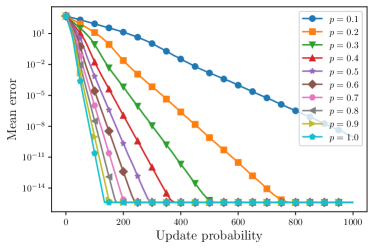
Figure 2: Mean errors for different update probabilities.

Table I further reports the empirical convergence rate (estimated by computing the slope of the mean error curves in Figure 2) attained for the different update probabilities.

TABLE I: Empirical convergence rate for different update probabilities.

Update probability	Convergence rate
$0.1$	$0.972$
$0.2$	$0.944$
$0.3$	$0.917$
$0.4$	$0.889$
$0.5$	$0.861$
$0.6$	$0.834$
$0.7$	$0.807$
$0.8$	$0.779$
$0.9$	$0.750$
$1.0$	$0.723$

VI-B Additive errors

We evaluate now the effect of additive errors on the performance of Algorithm 1, in a fully synchronous case ($p_{i}=1$). In particular, each local update to $x_{i}^{\ell}$ (line $5$ in the pseudo-code) is subject to an additive error $e_{i}^{\ell}$ whose components are drawn from the Weibull distribution . With this choice, by Lemma 11 we know that the norm of $e_{i}^{\ell}$ is sub-Weibull and thus satisfies Assumption 1(ii).

Lemma 11 (Norm of sub-Weibull vectors).

Let $e=[e_{1},\ldots,e_{p}]^{\top}$ be a random vector in $\mathbb{R}^{p}$, $p<+\infty$, such that $e_{i}\sim\mathrm{subW}(\theta,\nu)$, $i=1,\ldots,p$. Then the Euclidean norm of $e$ is sub-Weibull with

$$\left\lVert e\right\rVert\sim\mathrm{subW}(\theta,\max\{1,2^{\theta}\}\sqrt{p}\nu).$$

Proof.

We want to characterize $\left\lVert e\right\rVert=\sqrt{\sum_{i=1}^{p}e_{i}^{2}}$ as a sub-Weibull. By Lemma 8 we know that $e_{i}^{2}\sim\mathrm{subW}(2\theta,\max\{1,2^{2\theta}\}\nu^{2})$, and it follows that $\sum_{i=1}^{p}e_{i}^{2}\sim\mathrm{subW}(2\theta,p\max\{1,2^{2\theta}\}\nu^{2})$. Finally, taking the square root and simplifying yields the thesis. ∎

In Table II we report the mean asymptotic error (computed as the maximum mean error in the last $4/5$ of the simulation) for different values of $\theta$ and $\nu$. In accordance with the theoretical results (cf. Proposition 3), the heavier the tail (i.e. the larger $\theta$) or the larger the scaling parameter $\nu$, the larger the error attained by the algorithm.

TABLE II: Asymptotic error for different sub-Weibull distributions of the additive noise.

	$10^{-2}$	$10^{-1}$	$1$
$\theta=1/2$	$7.297\times 10^{-2}$	$7.613\times 10^{-1}$	$1.452\times 10^{1}$
$1$	$8.408\times 10^{-2}$	$8.802\times 10^{-1}$	$1.719\times 10^{1}$
$2$	$1.807\times 10^{-1}$	$2.096\times 10^{0}$	$4.160\times 10^{1}$

Appendix A Proof of Lemma 8

Proof of 1) The result follows by $\left\lVert ax\right\rVert_{k}=|a|\left\lVert x\right\rVert_{k}\leq|a|\nu k^{\theta}$.

Proof of 2) For completeness we report the proof provided in [32, Proposition 3]. Using the triangle inequality we write

$$\left\lVert x_{1}+x_{2}\right\rVert_{k} \leq\left\lVert x_{1}\right\rVert_{k}+\left\lVert x_{2}\right\rVert_{k}\overset{\text{(i)}}{\leq}\nu_{1}k^{\theta_{1}}+\nu_{2}k^{\theta_{2}}$$

$$\overset{\text{(ii)}}{\leq}(\nu_{1}+\nu_{2})k^{\max\{\theta_{1},\theta_{2}\}},$$

where (i) holds by the assumption that $x_{i}$ are sub-Weibull, and (ii) holds since $k\geq 1$.

Proof of 3) By definition of $\left\lVert\cdot\right\rVert_{k}$ we can write

$$\left\lVert xy\right\rVert_{k} \leq\mathbb{E}\left[|x|^{k}|y|^{k}\right]^{1/k}\overset{\text{(i)}}{=}\mathbb{E}\left[|x|^{k}\right]^{1/k}\mathbb{E}\left[|y|^{k}\right]^{1/k}$$

$$\overset{\text{(ii)}}{\leq}\nu_{1}k^{\theta_{1}}\nu_{2}k^{\theta_{2}}=\nu_{1}\nu_{2}k^{\theta_{1}+\theta_{2}}$$

where (i) holds by independence and (ii) by sub-Weibull assumption.

Proof of 4) By definition of $\left\lVert\cdot\right\rVert_{k}$ we have $\left\lVert x^{a}\right\rVert_{k}=\mathbb{E}\left[|x^{a}|^{k}\right]^{1/k}=\mathbb{E}\left[|x|^{ak}\right]^{1/k}$. Now, we distinguish two cases: if $0<a<1$ then by Jensen’s inequality we have

$$\mathbb{E}\left[|x|^{ak}\right]^{1/k}\leq\left(\mathbb{E}\left[|x|^{k}\right]^{1/k}\right)^{a}\leq(\nu k^{\theta})^{a};$$

instead if $a\geq 1$ then we can write

$$\mathbb{E}\left[|x|^{ak}\right]^{1/k}=\left(\mathbb{E}\left[|x|^{ak}\right]^{1/ak}\right)^{a}\overset{\text{(i)}}{\leq}\left(\nu(ak)^{\theta}\right)^{a}=\nu^{a}a^{a\theta}k^{\theta}$$

where (i) holds by the fact that $ak\geq 1$ and that $x$ is sub-Weibull. ∎

Appendix B Algorithm 1

B-A Derivation of the algorithm

Let us start from equation 8, characterized by

$$z^{\ell+1}=\frac{1}{n}\sum_{i=1}^{n}\left(z^{\ell}-\gamma\nabla f_{i}(z^{\ell})\right),\quad\ell\in\mathbb{N},$$

where we replaced $x$ with $z$. Defining the local states

$$x_{i}^{\ell+1}=\mathcal{G}_{i}z^{\ell}=z^{\ell}-\gamma\nabla f_{i}(z^{\ell}),\quad i=1,\ldots,n$$

we can then rewrite the update as $z^{\ell+1}=\frac{1}{n}\sum_{i=1}^{n}x_{i}^{\ell+1}.$

Consider now the asynchronous set-up described in section III-A, in which only the subset $\mathbb{I}^{\ell}$ of the agents is active. In this case, we need to modify the local update as follows

$$x_{i}^{\ell+1}=\begin{cases}\mathcal{G}_{i}z^{\ell}&\text{if}\ i\in\mathbb{I}^{\ell}\\ x_{i}^{\ell}&\text{otherwise},\end{cases}$$

so that only the active agents update their state. Since the coordinator receives new information only from the active agents, then we can modify its update as

$$z^{\ell+1}=\frac{1}{n}\left(\sum_{i\in\mathbb{I}^{\ell}}x_{i}^{\ell+1}+\sum_{i\not\in\mathbb{I}^{\ell}}x_{i}^{\ell}\right).$$

With this update, the coordinator aggregates the new information received from $\mathbb{I}^{\ell}$ with the most recent information received from the inactive agents (which may have been transmitted several iterations ago, e.g. if $x_{i}^{\ell+1}=x_{i}^{\ell}=x_{i}^{\ell-1}$).

B-B Interpretation as stochastic operator

The goal now is to show that Algorithm 1 derived in the previous section can be interpreted as a stochastic operator that fits into the framework of the paper.

We start with the deterministic algorithm (all agents are always active). Using $z^{\ell}=\frac{1}{n}\sum_{i=1}^{n}x_{i}^{\ell}$, the algorithm is described as

$$x_{i}^{\ell+1}=\mathcal{G}_{i}\left(\frac{1}{n}\sum_{j=1}^{n}x_{j}^{\ell}\right).$$

Letting $\mathbold{x}=(x_{1},\ldots,x_{n})$ the overall algorithm therefore is characterized by the update $\mathbold{x}^{\ell+1}=\mathcal{T}\mathbold{x}^{\ell}=(\mathcal{G}\circ\mathcal{A})\mathbold{x}^{\ell}$ with $\circ$ denoting composition of operators, and where $\mathcal{G}\mathbold{x}=(\mathcal{G}_{1}x_{1},\ldots,\mathcal{G}_{n}x_{n})$ and

$$\mathcal{A}\mathbold{x}=\left(\frac{1}{n}\sum_{i=1}^{n}x_{i},\ldots,\frac{1}{n}\sum_{i=1}^{n}x_{i}\right).$$

Let us now turn to the asynchronous set-up in which only the active agents $\mathbb{I}^{\ell}$ perform an update. Letting $u_{i}^{\ell}$ be a Bernoulli r.v. which is $1$ if agent $i$ updates at time $\ell$, then we can write

$$x_{i}^{\ell+1}=(1-u_{i}^{\ell})x_{i}^{\ell}+\mathcal{T}_{i}\mathbold{x}^{\ell},$$

which fits exactly into the framework of section III-B.

We conclude this section by discussing the properties of $\mathcal{T}$ as derived from the properties of the problem

$$\min_{x_{i}\in\mathbb{R}^{p}}\sum_{i=1}^{n}f_{i}(x_{i})\quad\text{s.t.}\ x_{1}=x_{2}=\ldots=x_{n}.$$

We remark first that $\mathcal{A}$ is non-expansive, and we need to characterize the properties of $\mathcal{G}$. Assume that the local costs have $\bar{\lambda}$-Lipschitz continuous gradients, and that they are $\underaccent{\bar}{\lambda}$-strongly convex, where we allow $\underaccent{\bar}{\lambda}=0$ to signify that the costs are convex. Then we have the following cases:

• convex costs ($\underaccent{\bar}{\lambda}=0$): if $\gamma<2/\bar{\lambda}$ then $\mathcal{G}$ is averaged, and hence so is $\mathcal{T}$ [21, section 3.3];

• strongly convex costs ($\underaccent{\bar}{\lambda}>0$): if $\gamma<2/\bar{\lambda}$ then $\mathcal{G}$ is contractive and by [49, Lemma 4.11] so is $\mathcal{T}$.

Finally, notice that the fixed point(s) of $\mathcal{T}$ do not coincide with solutions of the optimization problem, but rather given $\bar{\mathbold{x}}\in\operatorname{fix}(\mathcal{T})$ then

$$\bar{z}=\frac{1}{n}\sum_{i=1}^{n}\bar{x}_{i}$$

is a solution to the problem.

Appendix C Proofs of Section IV

C-A Proof of Proposition 1

Similarly to e.g. [27, 4], the first step is to define the norm

$${\left|\left|\left|\mathbold{x}\right|\right|\right|}:=\sqrt{\sum_{i=1}^{n}\frac{1}{p_{i}}\left\lVert x_{i}\right\rVert_{i}^{2}}$$

for which, letting $\bar{p}:=\max_{i}p_{i}$ and $\underaccent{\bar}{p}=\min_{i}p_{i}$, it holds that

$$\underaccent{\bar}{p}{\left|\left|\left|\mathbold{x}\right|\right|\right|}^{2}\leq\left\lVert\mathbold{x}\right\rVert^{2}\leq\bar{p}{\left|\left|\left|\mathbold{x}\right|\right|\right|}^{2}.$$ (12)

By the triangle inequality and the fact that ${\left|\left|\left|(u_{1}^{\ell}e_{1}^{\ell},\ldots,u_{n}^{\ell}e_{n}^{\ell})\right|\right|\right|}\leq{\left|\left|\left|\mathbold{e}^{\ell}\right|\right|\right|}$ we have

$${\left|\left|\left|\mathbold{x}^{\ell+1}-\bar{\mathbold{x}}^{\ell+1}\right|\right|\right|}\leq{\left|\left|\left|\hat{\mathcal{T}}^{\ell+1}\mathbold{x}^{\ell}-\bar{\mathbold{x}}^{\ell+1}\right|\right|\right|}+{\left|\left|\left|\mathbold{e}^{\ell}\right|\right|\right|}$$

where $\hat{\mathcal{T}}^{\ell+1}$ is defined in equation 9. Taking the expected value, by (12) we have $\mathbb{E}\left[{\left|\left|\left|\mathbold{e}^{\ell}\right|\right|\right|}\right]\leq\mathbb{E}\left[\left\lVert\mathbold{e}^{\ell}\right\rVert\right]/\sqrt{\underaccent{\bar}{p}}$, and by Assumption 1(ii) we have $\mathbb{E}\left[\left\lVert\mathbold{e}^{\ell}\right\rVert\right]\leq\nu$, hence $\mathbb{E}\left[{\left|\left|\left|\mathbold{e}^{\ell}\right|\right|\right|}\right]\leq\nu/\sqrt{\underaccent{\bar}{p}}.$ We focus now on the first term. By the law of total expectation and Jensen’s inequality we have

$$\mathbb{E}\left[{\left|\left|\left|\hat{\mathcal{T}}^{\ell+1}\mathbold{x}^{\ell}-\bar{\mathbold{x}}^{\ell+1}\right|\right|\right|}\right]=\mathbb{E}\left[\mathbb{E}_{\ell}\left[{\left|\left|\left|\hat{\mathcal{T}}^{\ell+1}\mathbold{x}^{\ell}-\bar{\mathbold{x}}^{\ell+1}\right|\right|\right|}\right]\right]$$

$$\hskip 85.35826pt\leq\mathbb{E}\left[\sqrt{\mathbb{E}_{\ell}\left[{\left|\left|\left|\hat{\mathcal{T}}^{\ell+1}\mathbold{x}^{\ell}-\bar{\mathbold{x}}^{\ell+1}\right|\right|\right|}^{2}\right]}\right]$$

where $\mathbb{E}_{\ell}\left[\cdot\right]$ denotes the expectation conditioned on $\mathbold{x}^{\ell}$. By linearity of the expected value we can write

$$\mathbb{E}_{\ell}\left[{\left|\left|\left|\hat{\mathcal{T}}^{\ell+1}\mathbold{x}^{\ell}-\bar{\mathbold{x}}^{\ell+1}\right|\right|\right|}^{2}\right]=$$

$$=\sum_{i=1}^{n}\mathbb{E}_{\ell}\left[\frac{1}{p_{i}}\left\lVert\hat{\mathcal{T}}_{i}^{\ell+1}\mathbold{x}^{\ell}-\bar{x}_{i}^{\ell+1}\right\rVert_{i}^{2}\right]$$

$$\overset{(a)}{=}\sum_{i=1}^{n}\mathbb{E}_{\ell}\left[\frac{u_{i}^{\ell}}{p_{i}}\left\lVert\mathcal{T}_{i}^{\ell+1}\mathbold{x}^{\ell}-\bar{x}_{i}^{\ell+1}\right\rVert_{i}^{2}+\frac{1-u_{i}^{\ell}}{p_{i}}\left\lVert x_{i}^{\ell}-\bar{x}_{i}^{\ell+1}\right\rVert_{i}^{2}\right]$$

$$\overset{(b)}{=}\left\lVert\mathcal{T}^{\ell+1}\mathbold{x}^{\ell}-\bar{\mathbold{x}}^{\ell+1}\right\rVert^{2}+\sum_{i=1}^{n}\frac{1-p_{i}}{p_{i}}\left\lVert x_{i}^{\ell}-\bar{x}_{i}^{\ell+1}\right\rVert_{i}^{2}$$ (13)

$$\overset{(c)}{\leq}\zeta^{2}\left\lVert\mathbold{x}^{\ell}-\bar{\mathbold{x}}^{\ell+1}\right\rVert^{2}+\sum_{i=1}^{n}\frac{1-p_{i}}{p_{i}}\left\lVert x_{i}^{\ell}-\bar{x}_{i}^{\ell+1}\right\rVert_{i}^{2}$$

$$=\sum_{i=1}^{n}\frac{1}{p_{i}}(1-p_{i}+p_{i}\zeta^{2})\left\lVert x_{i}^{\ell}-\bar{x}_{i}^{\ell}\right\rVert_{i}^{2}$$

$$\overset{(d)}{\leq}\chi^{2}{\left|\left|\left|\mathbold{x}^{\ell}-\bar{\mathbold{x}}^{\ell}\right|\right|\right|}^{2}$$

where ($a$) holds by definition of $\hat{\mathcal{T}}^{\ell+1}$, ($b$) by the fact that $u_{i}^{\ell}\sim Ber(p_{i})$, ($c$) holds by the contractiveness in Assumption 2(i), and ($d$) by defining $\chi=\sqrt{\max_{i}1-p_{i}+p_{i}\zeta^{2}}=\sqrt{1-\underaccent{\bar}{p}+\underaccent{\bar}{p}\zeta^{2}}$.

Putting this bound together with that for $\mathbb{E}\left[{\left|\left|\left|\mathbold{e}^{\ell}\right|\right|\right|}\right]$:

$$\mathbb{E}\left[{\left|\left|\left|\mathbold{x}^{\ell+1}-\bar{\mathbold{x}}^{\ell+1}\right|\right|\right|}\right] \leq\chi\mathbb{E}\left[{\left|\left|\left|\mathbold{x}^{\ell}-\bar{\mathbold{x}}^{\ell+1}\right|\right|\right|}\right]+\nu/\sqrt{\underaccent{\bar}{p}}$$

$$\leq\chi\mathbb{E}\left[{\left|\left|\left|\mathbold{x}^{\ell}-\bar{\mathbold{x}}^{\ell}\right|\right|\right|}\right]+\chi\sigma+\nu/\sqrt{\underaccent{\bar}{p}}$$ (14)

where the last inequality holds by triangle inequality and Assumption 2(ii). Iterating and using the geometric sum

$$\mathbb{E}\left[{\left|\left|\left|\mathbold{x}^{\ell}-\bar{\mathbold{x}}^{\ell}\right|\right|\right|}\right]\leq\chi^{\ell}{\left|\left|\left|\mathbold{x}^{0}-\bar{\mathbold{x}}^{0}\right|\right|\right|}+\frac{1-\chi^{\ell}}{1-\chi}(\chi\sigma+\frac{\nu}{\sqrt{\underaccent{\bar}{p}}}),$$

and the thesis follows by equation 12. ∎

C-B Proof of Proposition 2

Let $\langle\mkern-2.5mu\langle\cdot\rangle\mkern-2.5mu\rangle$ be the inner product that induces ${\left|\left|\left|\cdot\right|\right|\right|}$, then we can write

$${\left|\left|\left|\mathbold{x}^{\ell+1}-\bar{\mathbold{x}}^{\ell+1}\right|\right|\right|}^{2}=$$

$$={\left|\left|\left|\hat{\mathcal{T}}^{\ell+1}\mathbold{x}^{\ell}-\bar{\mathbold{x}}^{\ell+1}\right|\right|\right|}^{2}+{\left|\left|\left|(u_{1}^{\ell}e_{1}^{\ell},\ldots,u_{n}^{\ell}e_{n}^{\ell})\right|\right|\right|}^{2}+$$

$$+\langle\mkern-2.5mu\langle\hat{\mathcal{T}}^{\ell+1}\mathbold{x}^{\ell}-\bar{\mathbold{x}}^{\ell+1},(u_{1}^{\ell}e_{1}^{\ell},\ldots,u_{n}^{\ell}e_{n}^{\ell})\rangle\mkern-2.5mu\rangle$$

$$\leq{\left|\left|\left|\hat{\mathcal{T}}^{\ell+1}\mathbold{x}^{\ell}-\bar{\mathbold{x}}^{\ell+1}\right|\right|\right|}^{2}+{\left|\left|\left|\mathbold{e}^{\ell}\right|\right|\right|}^{2}+2\operatorname{diam}(\mathbb{D}){\left|\left|\left|\mathbold{e}^{\ell}\right|\right|\right|}$$

where the last inequality follows by ${\left|\left|\left|(u_{1}^{\ell}e_{1}^{\ell},\ldots,u_{n}^{\ell}e_{n}^{\ell})\right|\right|\right|}\leq{\left|\left|\left|\mathbold{e}^{\ell}\right|\right|\right|}$ and by Cauchy-Schwarz inequality. Using the law of total expectation we can write $\mathbb{E}\left[{\left|\left|\left|\hat{\mathcal{T}}^{\ell+1}\mathbold{x}^{\ell}-\bar{\mathbold{x}}^{\ell+1}\right|\right|\right|}^{2}\right]=\mathbb{E}\left[\mathbb{E}_{\ell}\left[{\left|\left|\left|\hat{\mathcal{T}}^{\ell+1}\mathbold{x}^{\ell}-\bar{\mathbold{x}}^{\ell+1}\right|\right|\right|}^{2}\right]\right]$ where recall that $\mathbb{E}_{\ell}\left[\cdot\right]$ is conditioned on $\mathbold{x}^{\ell}$. Following the steps leading to equation 13 we have

$$\mathbb{E}_{\ell}\left[{\left|\left|\left|\hat{\mathcal{T}}^{\ell+1}\mathbold{x}^{\ell}-\bar{\mathbold{x}}^{\ell+1}\right|\right|\right|}^{2}\right]=$$

$$=\left\lVert\mathcal{T}^{\ell+1}\mathbold{x}^{\ell}-\bar{\mathbold{x}}^{\ell+1}\right\rVert^{2}+\sum_{i=1}^{n}\frac{1-p_{i}}{p_{i}}\left\lVert x_{i}^{\ell}-\bar{x}_{i}^{\ell+1}\right\rVert_{i}^{2}$$

$$\overset{(a)}{\leq}\left\lVert\mathbold{x}^{\ell}-\bar{\mathbold{x}}^{\ell+1}\right\rVert^{2}-\frac{1-\alpha}{\alpha}\left\lVert(\mathcal{I}-\mathcal{T}^{\ell+1})\mathbold{x}^{\ell}\right\rVert^{2}+$$

$$\hskip 42.67912pt+\sum_{i=1}^{n}\frac{1-p_{i}}{p_{i}}\left\lVert x_{i}^{\ell}-\bar{x}_{i}^{\ell+1}\right\rVert_{i}^{2}$$

$$={\left|\left|\left|\mathbold{x}^{\ell}-\bar{\mathbold{x}}^{\ell+1}\right|\right|\right|}^{2}-\frac{1-\alpha}{\alpha}\left\lVert(\mathcal{I}-\mathcal{T}^{\ell+1})\mathbold{x}^{\ell}\right\rVert^{2}$$

where ($a$) follows by averagedness in Assumption 3(i). Let $\bar{\mathbold{x}}^{\ell}\in\operatorname{fix}(\mathcal{T}^{\ell})$, then

$${\left|\left|\left|\mathbold{x}^{\ell}-\bar{\mathbold{x}}^{\ell+1}\right|\right|\right|}^{2}={\left|\left|\left|\mathbold{x}^{\ell}-\bar{\mathbold{x}}^{\ell}\right|\right|\right|}^{2}+{\left|\left|\left|\bar{\mathbold{x}}^{\ell}-\bar{\mathbold{x}}^{\ell+1}\right|\right|\right|}^{2}+$$

$$\hskip 56.9055pt+2\langle\mkern-2.5mu\langle\mathbold{x}^{\ell}-\bar{\mathbold{x}}^{\ell},\bar{\mathbold{x}}^{\ell}-\bar{\mathbold{x}}^{\ell+1}\rangle\mkern-2.5mu\rangle$$

$$\leq{\left|\left|\left|\mathbold{x}^{\ell}-\bar{\mathbold{x}}^{\ell}\right|\right|\right|}^{2}+\sigma^{2}/\underaccent{\bar}{p}+2\operatorname{diam}(\mathbb{D})\sigma/\sqrt{\underaccent{\bar}{p}}$$

where we used Assumption 3(ii), equation 12, and the fact that $\mathbb{D}$ is bounded. Putting all these results together yields

$$\mathbb{E}\left[{\left|\left|\left|\mathbold{x}^{\ell+1}-\bar{\mathbold{x}}^{\ell+1}\right|\right|\right|}^{2}\right]\leq\mathbb{E}\left[{\left|\left|\left|\mathbold{x}^{\ell}-\bar{\mathbold{x}}^{\ell}\right|\right|\right|}^{2}\right]+\sigma^{2}/\underaccent{\bar}{p}+$$

$$+2\operatorname{diam}(\mathbb{D})\sigma/\sqrt{\underaccent{\bar}{p}}+\mathbb{E}\left[{\left|\left|\left|\mathbold{e}^{\ell}\right|\right|\right|}^{2}+2\operatorname{diam}(\mathbb{D}){\left|\left|\left|\mathbold{e}^{\ell}\right|\right|\right|}\right]+$$

$$-\frac{1-\alpha}{\alpha}\left\lVert(\mathcal{I}-\mathcal{T}^{\ell+1})\mathbold{x}^{\ell}\right\rVert^{2}$$

$$\leq\mathbb{E}\left[{\left|\left|\left|\mathbold{x}^{\ell}-\bar{\mathbold{x}}^{\ell}\right|\right|\right|}^{2}\right]+d-\frac{1-\alpha}{\alpha}\left\lVert(\mathcal{I}-\mathcal{T}^{\ell+1})\mathbold{x}^{\ell}\right\rVert^{2}$$ (15)

where the bound

$$d:=\frac{1}{\underaccent{\bar}{p}}\left(\sigma^{2}+4^{\theta}\nu^{2}\right)+\frac{2\operatorname{diam}(\mathbb{D})}{\sqrt{\underaccent{\bar}{p}}}\left(\sigma+\nu\right)$$

was derived using Lemma 8 to show that ${\left|\left|\left|\mathbold{e}^{\ell}\right|\right|\right|}^{2}\sim\mathrm{subW}(2\theta,4^{\theta}\nu^{2}/\underaccent{\bar}{p})$ and ${\left|\left|\left|\mathbold{e}^{\ell}\right|\right|\right|}\sim\mathrm{subW}(\theta,\nu/\sqrt{\underaccent{\bar}{p}})$, and using the fact that the second parameter of a sub-Weibull provides a bound to the mean of the random variable (cf. Remark 2).

Reordering equation 15 and averaging over time yields

$$\frac{1}{\ell+1}\sum_{h=0}^{\ell}\mathbb{E}\left[\left\lVert(\mathcal{I}-\mathcal{T}^{h})\mathbold{x}^{h}\right\rVert^{2}\right]\leq$$

$$\leq\frac{\alpha}{1-\alpha}\left(\frac{1}{\ell+1}{\left|\left|\left|\mathbold{x}^{0}-\bar{\mathbold{x}}^{0}\right|\right|\right|}^{2}+d\right)$$

where we used the telescopic sum and removed the negative term $-\mathbb{E}\left[{\left|\left|\left|\mathbold{x}^{\ell+1}-\bar{\mathbold{x}}^{\ell+1}\right|\right|\right|}^{2}\right]$. The thesis follows by equation 12 and $\sqrt{\underaccent{\bar}{p}}\leq 1$. ∎

C-C Proof of Corollary 1

By Proposition 1 we know that

$$\mathbb{E}\left[\left\lVert\mathbold{x}^{\ell}-\bar{\mathbold{x}}^{\ell}\right\rVert\right]\leq\sqrt{\frac{\bar{p}}{\underaccent{\bar}{p}}}\left(\chi^{\ell}\left\lVert\mathbold{x}^{0}-\bar{\mathbold{x}}^{0}\right\rVert+\frac{1-\chi^{\ell}}{1-\chi}(\chi\sigma+\nu)\right)$$

and, defining the random variable

$$y^{\ell}:=\max\left\{0,\sqrt{\frac{\underaccent{\bar}{p}}{\bar{p}}}\left\lVert\mathbold{x}^{\ell}-\bar{\mathbold{x}}^{\ell}\right\rVert-\frac{1-\chi^{\ell}}{1-\chi}(\chi\sigma+\nu)\right\},$$

this fact implies $\mathbb{E}\left[y^{\ell}\right]\leq\chi^{\ell}\left\lVert\mathbold{x}^{0}-\bar{\mathbold{x}}^{0}\right\rVert$.

By Markov’s inequality then we have that, for any $\epsilon>0$: $\mathbb{P}\left[y^{\ell}\geq\epsilon\right]\leq\mathbb{E}\left[y^{\ell}\right]/\epsilon\leq\chi^{\ell}\left\lVert\mathbold{x}^{0}-\bar{\mathbold{x}}^{0}\right\rVert/\epsilon,$ and summing over time yields

$$\sum_{\ell=0}^{\infty}\mathbb{P}\left[y^{\ell}\geq\epsilon\right]\leq\frac{1}{1-\chi}\frac{\left\lVert\mathbold{x}^{0}-\bar{\mathbold{x}}^{0}\right\rVert}{\epsilon}<\infty.$$

By the Borel-Cantelli lemma, this fact implies that almost surely $\limsup_{\ell\to\infty}y^{\ell}\leq\epsilon,$ and, since the inequality holds for any $\epsilon>0$ the thesis is proved. ∎

C-D Proof of Corollary 2

By assumption (ii) the operator is static, which implies that $\sigma=0$; hereafter $\bar{\mathbold{x}}$ denotes the unique fixed point of $\mathcal{T}$.

Following the same derivation leading to (14) yields

$$\mathbb{E}\left[{\left|\left|\left|\mathbold{x}^{\ell+1}-\bar{\mathbold{x}}\right|\right|\right|}\right]\leq\chi\mathbb{E}\left[{\left|\left|\left|\mathbold{x}^{\ell}-\bar{\mathbold{x}}\right|\right|\right|}\right]+\nu^{\ell}/\sqrt{\underaccent{\bar}{p}}$$

with the difference that now the right-most term is a function of $\ell$ as well. Iterating and using equation 12 we have

$$\mathbb{E}\left[\left\lVert\mathbold{x}^{\ell}-\bar{\mathbold{x}}\right\rVert\right]\leq\sqrt{\frac{\bar{p}}{\underaccent{\bar}{p}}}\left(\chi^{\ell}\left\lVert\mathbold{x}^{0}-\bar{\mathbold{x}}\right\rVert+\sum_{h=0}^{\ell-1}\chi^{\ell-h-1}\nu^{h}\right).$$

Similarly to Corollary 1, by Markov’s inequality we have

$$\lim_{\ell\to\infty}\left\lVert\mathbold{x}^{\ell}-\bar{\mathbold{x}}\right\rVert\leq\sqrt{\frac{\bar{p}}{\underaccent{\bar}{p}}}\lim_{\ell\to\infty}\sum_{h=0}^{\ell-1}\chi^{\ell-h-1}\nu^{h}=0$$

where the right-hand side is equal to zero since $\{\nu^{\ell}\}_{\ell\in\mathbb{N}}$ is summable and we can apply [50, Lemma 3.1(a)] because $\chi\in(0,1)$. ∎

Appendix D Proofs of Section V

D-A Proof of Proposition 3

By the triangle inequality and the fact that $\left\lVert(\ldots,u_{i}^{\ell}e_{i}^{\ell},\ldots)\right\rVert\leq\left\lVert\mathbold{e}^{\ell}\right\rVert$ we have

$$\left\lVert\mathbold{x}^{\ell+1}-\bar{\mathbold{x}}^{\ell+1}\right\rVert\leq\left\lVert\hat{\mathcal{T}}^{\ell+1}\mathbold{x}^{\ell}-\bar{\mathbold{x}}^{\ell+1}\right\rVert+\left\lVert\mathbold{e}^{\ell}\right\rVert.$$

By Assumption 4 we know that almost surely $\left\lVert\hat{\mathcal{T}}^{\ell+1}\mathbold{x}^{\ell}-\bar{\mathbold{x}}^{\ell+1}\right\rVert\leq\left\lVert\mathbold{x}^{\ell}-\bar{\mathbold{x}}^{\ell+1}\right\rVert$; therefore, letting $p:=\prod_{i=1}^{n}p_{i}$ and using contractiveness, we can write

$$\left\lVert\hat{\mathcal{T}}^{\ell+1}\mathbold{x}^{\ell}-\bar{\mathbold{x}}^{\ell+1}\right\rVert \leq\begin{cases}\zeta\left\lVert\mathbold{x}^{\ell}-\bar{\mathbold{x}}^{\ell+1}\right\rVert&\text{w.p.}\ p\\ \left\lVert\mathbold{x}^{\ell}-\bar{\mathbold{x}}^{\ell+1}\right\rVert&\text{w.p.}\ 1-p\end{cases}$$

$$\leq\zeta^{u^{\ell}}\left\lVert\mathbold{x}^{\ell}-\bar{\mathbold{x}}^{\ell+1}\right\rVert$$

where $u^{\ell}\sim Ber(p)$. As a consequence:

$$\left\lVert\mathbold{x}^{\ell+1}-\bar{\mathbold{x}}^{\ell+1}\right\rVert \leq\zeta^{u^{\ell}}\left\lVert\mathbold{x}^{\ell}-\bar{\mathbold{x}}^{\ell+1}\right\rVert+\left\lVert\mathbold{e}^{\ell}\right\rVert$$

$$\leq\zeta^{u^{\ell}}\left\lVert\mathbold{x}^{\ell}-\bar{\mathbold{x}}^{\ell}\right\rVert+\zeta^{u^{\ell}}\sigma+\left\lVert\mathbold{e}^{\ell}\right\rVert,$$

where the second inequality holds by Assumption 2(ii). Iterating we get

$$\begin{split}\left\lVert\mathbold{x}^{\ell+1}-\bar{\mathbold{x}}^{\ell+1}\right\rVert&\leq\zeta^{\sum_{h=0}^{\ell}u^{h}}\left\lVert\mathbold{x}^{0}-\bar{\mathbold{x}}^{0}\right\rVert+\\ &+\sum_{h=0}^{\ell}\zeta^{\sum_{j=h+1}^{\ell}u^{j}}(\zeta^{u^{\ell}}\sigma+\left\lVert\mathbold{e}^{h}\right\rVert).\end{split}$$ (16)

The goal now is to prove that the right-hand side of equation 16 is a sub-Weibull random variable. First of all, by Lemma 9 below, we know that $\zeta^{\sum_{h=0}^{\ell}u^{h}}\sim\mathrm{subW}(1/2,\eta(\ell))$, where $\eta(\ell)\in[0,1)$ and $\lim_{\ell\to\infty}\eta(\ell)=0$. But by Assumption 1(ii) $\left\lVert\mathbold{e}^{\ell}\right\rVert\sim\mathrm{subW}(\theta,\nu)$, and using Lemma 8 yields

$$\sum_{h=0}^{\ell} \zeta^{\sum_{j=h+1}^{\ell}u^{j}}\left\lVert\mathbold{e}^{h}\right\rVert\sim$$

$$\sim\mathrm{subW}\left(\max\{1/2,\theta\},\nu\sum_{h=0}^{\ell}\eta(\ell-h-1)\right).$$

We need now prove that $\sum_{h=0}^{\ell}\zeta^{\sum_{j=h+1}^{\ell}u^{j}}\zeta^{u^{\ell}}\sigma$ is also sub-Weibull. Let $\beta(\ell)=\sum_{h=0}^{\ell}u^{h}$ be the binomial r.v. counting the $u^{h}=1$, and define the sub-sequence $\{h_{k}\}_{k=0}^{\beta_{i}(\ell)-1}$ with $u^{h_{k}}=1$ for $k=0,\ldots,\beta_{i}(\ell)-1$. Then

$$\sum_{h=0}^{\ell}\zeta^{\sum_{j=h+1}^{\ell}u^{j}}\zeta^{u^{\ell}} =\sum_{k=0}^{\beta(\ell)}\zeta^{k}\sum_{h=h_{k}}^{h_{k+1}-1}1=\sum_{k=0}^{\beta(\ell)}\zeta^{k}(h_{k+1}-h_{k})$$

$$\leq\sum_{k=0}^{\ell}\zeta^{k}(h_{k+1}-h_{k})$$

where $y_{k}:=h_{k+1}-h_{k}$ is a geometric r.v., which we want to characterize as a sub-Weibull. Notice that $y_{k}$ counts the number of failures ($u^{h}=0$) between $h_{k}$ and $h_{k+1}$, and that $u^{h}\sim Ber(p)$. Since $y_{k}\leq z$, where $z$ is an exponential r.v. with rate $\log(1/(1-p))$, then $y_{k}\sim\mathrm{subW}(1,1/\log(1/(1-p)))$. We can now simplify the second sub-Weibull parameter of $y_{k}$ by using the inequality $\log(1+a)\geq a/(a+1)$, for $a>-1$, by which $1/\log(1/(1-p))\leq 1/p$. To conclude, we have $h_{k+1}-h_{k}\sim\mathrm{subW}(1,1/p)$. Using Lemma 8 and the geometric series then yields

$$\sum_{h=0}^{\ell}\zeta^{\sum_{j=h+1}^{\ell}u^{j}}\zeta^{u^{\ell}}\sigma\sim\mathrm{subW}\left(1,\frac{1-\zeta^{\ell}}{1-\zeta}\frac{\sigma}{p}\right).$$

We have now characterized the second term in the right-hand side of equation 16 as sub-Weibull, and by Lemma 9 we know that $\zeta^{\sum_{h=0}^{\ell}u^{h}}\left\lVert\mathbold{x}^{0}-\bar{\mathbold{x}}^{0}\right\rVert\sim\mathrm{subW}(1/2,\eta(\ell)\left\lVert\mathbold{x}^{0}-\bar{\mathbold{x}}^{0}\right\rVert)$, which implies overall:

$$\lx@cref{creftype~refnum}{eq:intermediate-bound-4}\sim \mathrm{subW}\Big{(}\max\{1,\theta\},$$

$$\eta(\ell)\left\lVert\mathbold{x}^{0}-\bar{\mathbold{x}}^{0}\right\rVert+\frac{1-\zeta^{\ell}}{1-\zeta}\frac{\sigma}{p}+\nu\sum_{h=0}^{\ell}\eta(\ell-h-1)\Big{)}.$$

Using Lemma 6 yields the thesis. ∎

D-B Proof of Lemma 9

By the fact that $\zeta\in(0,1)$, we know that $\zeta^{\beta(\ell)}\in[\zeta^{\ell},1]$, which means that $\zeta^{\beta(\ell)}$ is a bounded r.v.. As a consequence, we can model $\zeta^{\beta(\ell)}$ as a sub-Gaussian r.v., that is, a sub-Weibull with $\theta=1/2$, see Remark 3. The goal then is to characterize the $\nu$ sub-Weibull parameter of this r.v..

By the binomial distribution of $\beta(\ell)$ we have, for any $k\geq 1$

$$\left\lVert\zeta^{\beta(\ell)}\right\rVert_{k}^{k} =\mathbb{E}\left[(\zeta^{k})^{\beta(\ell)}\right]=\sum_{j=0}^{\ell}(\zeta^{k})^{j}\binom{\ell}{j}p^{j}(1-p)^{\ell-j}$$

$$=\sum_{j=0}^{\ell}\binom{\ell}{j}\left(\zeta^{k}p\right)^{j}(1-p)^{\ell-j}=(1-p+p\zeta^{k})^{\ell}$$

where the last equality holds by the binomial theorem. Taking the $k$-th root gives us $\left\lVert\zeta^{\beta(\ell)}\right\rVert_{k}=\left(1-p+p\zeta^{k}\right)^{\ell/k},$ and by definition (ii) in Lemma 5 this implies that the sub-Weibull parameter of $\zeta^{\beta(\ell)}$ satisfies (using $\theta=1/2$):

$$\eta(\ell)\geq\frac{\left(1-p+p\zeta^{k}\right)^{\ell/k}}{\sqrt{k}}.$$

The right-hand side is finite for any choice of $k\geq 1$, and choosing the maximum then yields the thesis. ∎

D-C Proof of Proposition 4

Using the definition of norm, the fact that $\left\lVert(\ldots,u_{i}^{\ell}e_{i}^{\ell},\ldots)\right\rVert\leq\left\lVert\mathbold{e}^{\ell}\right\rVert$, and Cauchy-Schwarz inequality we can write

$$\left\lVert\mathbold{x}^{\ell+1}-\bar{\mathbold{x}}^{\ell+1}\right\rVert^{2}\leq$$

$$\leq\left\lVert\hat{\mathcal{T}}^{\ell+1}\mathbold{x}^{\ell}-\bar{\mathbold{x}}^{\ell+1}\right\rVert^{2}+\left\lVert\mathbold{e}^{\ell}\right\rVert^{2}+2\operatorname{diam}(\mathbb{D})\left\lVert\mathbold{e}^{\ell}\right\rVert$$

where, by Assumption 4 and averagedness (Assumption 3(i)), we know that

$$\left\lVert\hat{\mathcal{T}}^{\ell+1}\mathbold{x}^{\ell}-\bar{\mathbold{x}}^{\ell+1}\right\rVert^{2}\leq$$

$$\qquad\leq\left\lVert\mathbold{x}^{\ell}-\bar{\mathbold{x}}^{\ell+1}\right\rVert^{2}-u^{\ell}\frac{1-\alpha}{\alpha}\left\lVert(\mathcal{I}-\mathcal{T}^{\ell+1})\mathbold{x}^{\ell}\right\rVert^{2}$$

with $p:=\prod_{i=1}^{n}p_{i}$ and $u^{\ell}\sim Ber(p)$.

Using Assumption 3(ii) and Cauchy-Schwarz inequality we can therefore write

$$\left\lVert\mathbold{x}^{\ell+1}-\bar{\mathbold{x}}^{\ell+1}\right\rVert^{2}\leq$$ (17)

$$\quad\leq\left\lVert\mathbold{x}^{\ell}-\bar{\mathbold{x}}^{\ell+1}\right\rVert^{2}-u^{\ell}\frac{1-\alpha}{\alpha}\left\lVert(\mathcal{I}-\mathcal{T}^{\ell+1})\mathbold{x}^{\ell}\right\rVert^{2}+$$

$$\quad+\left\lVert\mathbold{e}^{\ell}\right\rVert^{2}+2\operatorname{diam}(\mathbb{D})\left\lVert\mathbold{e}^{\ell}\right\rVert+\sigma^{2}+2\operatorname{diam}(\mathbb{D})\sigma.$$

Rearranging, averaging over time, and using the telescopic sum we have

$$\begin{split}&\frac{1}{\ell+1}\sum_{h=0}^{\ell}u^{h}\left\lVert(\mathcal{I}-\mathcal{T}^{h})\mathbold{x}^{h}\right\rVert^{2}\leq\\ &\qquad\leq\frac{1}{\ell+1}\frac{\alpha}{1-\alpha}\left(\left\lVert\mathbold{x}^{0}-\bar{\mathbold{x}}^{0}\right\rVert^{2}+\sum_{h=0}^{\ell}d^{h}\right)\end{split}$$ (18)

with $d^{h}:=\sigma^{2}+\left\lVert\mathbold{e}^{\ell}\right\rVert^{2}+2\operatorname{diam}(\mathbb{D})(\sigma+\left\lVert\mathbold{e}^{h}\right\rVert)$.

Now, by Lemma 8 and Assumption 1(ii) we know that

$$d^{h}\sim\mathrm{subW}\left(2\theta,\sigma^{2}+4^{\theta}\nu^{2}+2\operatorname{diam}(\mathbb{D})(\sigma+\nu)\right)$$

which implies that the right-hand side of equation 18 is sub-Weibull with parameters $2\theta$ and

$$\frac{\alpha}{1-\alpha}\left(\frac{1}{\ell+1}\left\lVert\mathbold{x}^{0}-\bar{\mathbold{x}}^{0}\right\rVert^{2}+\sigma^{2}+4^{\theta}\nu^{2}+2\operatorname{diam}(\mathbb{D})(\sigma+\nu)\right),$$

which yields the thesis by Lemma 6. ∎

D-D Proof of Proposition 6

Setting $\sigma=0$ and $\left\lVert\mathbold{e}^{\ell}\right\rVert=\bm{0}$ in equation 17 yields

$$\left\lVert\mathbold{x}^{\ell+1}-\bar{\mathbold{x}}\right\rVert^{2}\leq\left\lVert\mathbold{x}^{\ell}-\bar{\mathbold{x}}\right\rVert^{2}-u^{\ell}\frac{1-\alpha}{\alpha}\left\lVert(\mathcal{I}-\mathcal{T})\mathbold{x}^{\ell}\right\rVert^{2},$$ (19)

which implies $\left\lVert\mathbold{x}^{\ell+1}-\bar{\mathbold{x}}\right\rVert^{2}\leq\left\lVert\mathbold{x}^{\ell}-\bar{\mathbold{x}}\right\rVert^{2}$, that is, the operator is stochastic Fejér monotone [27, 28]. This means that the fixed point residual $\{\left\lVert(\mathcal{I}-\mathcal{T})\mathbold{x}^{\ell}\right\rVert\}_{\ell\in\mathbb{N}|u^{\ell}=1}$ is monotonically decreasing.

Therefore, summing equation 19 over time and using Fejér monotonicity we can write

$$\beta(\ell)\left\lVert(\mathcal{I}-\mathcal{T})\mathbold{x}^{\ell}\right\rVert^{2} \leq\sum_{h=0}^{\ell}u^{h}\left\lVert(\mathcal{I}-\mathcal{T})\mathbold{x}^{h}\right\rVert^{2}$$

$$\leq\frac{\alpha}{1-\alpha}\left\lVert\mathbold{x}^{0}-\bar{\mathbold{x}}\right\rVert^{2}$$

where we used the fact that the sequence $\{\left\lVert\mathbold{x}^{\ell+1}-\mathbold{x}^{\ell}\right\rVert\}_{\ell\in\mathbb{N}|u^{\ell}=1}$ has $\beta(\ell)$ non-zero terms. Dividing by $\beta(\ell)$ on both sides we get

$$\left\lVert\mathbold{x}^{\ell+1}-\mathbold{x}^{\ell}\right\rVert^{2}\leq\frac{1}{\beta(\ell)}\frac{\alpha}{1-\alpha}\left\lVert\mathbold{x}^{0}-\bar{\mathbold{x}}\right\rVert^{2}.$$

We have now the following fact

$$\mathbb{P}\left[\frac{1}{\beta(\ell)}\left\lVert\mathbold{x}^{0}-\bar{\mathbold{x}}\right\rVert^{2}\geq\frac{1}{(p-\epsilon)(\ell+1)}\left\lVert\mathbold{x}^{0}-\bar{\mathbold{x}}\right\rVert^{2}\right]=$$

$$=\mathbb{P}\left[\beta(\ell)\leq(\ell+1)(p-\epsilon)\right]\overset{\text{(i)}}{\leq}\exp\left(-(\ell+1)D(p-\epsilon||p)\right)$$

where (i) holds by Sanov’s theorem [47, Theorem D.3] (cf. [47, eq. (D.7)]), and the thesis follows. ∎

References

- [1] T. Li, A. K. Sahu, A. Talwalkar, and V. Smith, “Federated Learning: Challenges, Methods, and Future Directions,” IEEE Signal Processing Magazine, vol. 37, no. 3, pp. 50–60, May 2020.
- [2] T. Gafni, N. Shlezinger, K. Cohen, Y. C. Eldar, and H. V. Poor, “Federated Learning: A signal processing perspective,” IEEE Signal Processing Magazine, vol. 39, no. 3, pp. 14–41, May 2022.
- [3] Z. Peng, T. Wu, Y. Xu, M. Yan, and W. Yin, “Coordinate Friendly Structures, Algorithms and Applications,” Annals of Mathematical Sciences and Applications, vol. 1, no. 1, pp. 57–119, 2016.
- [4] P. Bianchi, W. Hachem, and F. Iutzeler, “A Coordinate Descent Primal-Dual Algorithm and Application to Distributed Asynchronous Optimization,” IEEE Transactions on Automatic Control, vol. 61, no. 10, pp. 2947–2957, 2016.
- [5] N. Bastianello, R. Carli, L. Schenato, and M. Todescato, “Asynchronous distributed optimization over lossy networks via relaxed admm: Stability and linear convergence,” IEEE Transactions on Automatic Control, vol. 66, no. 6, pp. 2620–2635, 2021.
- [6] S. Salzo and S. Villa, “Parallel random block-coordinate forward–backward algorithm: a unified convergence analysis,” Mathematical Programming, Apr. 2021.
- [7] R. Dixit, A. S. Bedi, R. Tripathi, and K. Rajawat, “Online Learning with Inexact Proximal Online Gradient Descent Algorithms,” IEEE Transactions on Signal Processing, vol. 67, no. 5, pp. 1338 – 1352, 2019.
- [8] S. Liu, P.-Y. Chen, B. Kailkhura, G. Zhang, A. O. Hero III, and P. K. Varshney, “A Primer on Zeroth-Order Optimization in Signal Processing and Machine Learning: Principals, Recent Advances, and Applications,” IEEE Signal Processing Magazine, vol. 37, no. 5, pp. 43–54, Sep. 2020.
- [9] L. Bottou, F. E. Curtis, and J. Nocedal, “Optimization methods for large-scale machine learning,” Siam Review, vol. 60, no. 2, pp. 223–311, 2018.
- [10] A. Simonetto, E. Dall’Anese, J. Monteil, and A. Bernstein, “Personalized optimization with user’s feedback,” Automatica, vol. 131, p. 109767, Sep. 2021.
- [11] J. C. Duchi, M. I. Jordan, M. J. Wainwright, and A. Wibisono, “Optimal Rates for Zero-Order Convex Optimization: The Power of Two Function Evaluations,” IEEE Transactions on Information Theory, vol. 61, no. 5, pp. 2788–2806, May 2015.
- [12] Y. Nesterov and V. Spokoiny, “Random Gradient-Free Minimization of Convex Functions,” Foundations of Computational Mathematics, vol. 17, no. 2, pp. 527–566, Apr. 2017.
- [13] A. S. Berahas, L. Cao, K. Choromanski, and K. Scheinberg, “A Theoretical and Empirical Comparison of Gradient Approximations in Derivative-Free Optimization,” Foundations of Computational Mathematics, vol. 22, no. 2, pp. 507–560, Apr. 2022.
- [14] S. Shalev-Shwartz, “Online Learning and Online Convex Optimization,” Foundations and Trends in Machine Learning, vol. 4, no. 2, pp. 107–194, 2011.
- [15] E. Dall’Anese, A. Simonetto, and A. Bernstein, “On the Convergence of the Inexact Running Krasnosel’skiĭ–Mann Method,” IEEE Control Systems Letters, vol. 3, no. 3, pp. 613–618, Jul. 2019.
- [16] A. Simonetto, E. Dall’Anese, S. Paternain, G. Leus, and G. B. Giannakis, “Time-Varying Convex Optimization: Time-Structured Algorithms and Applications,” Proceedings of the IEEE, vol. 108, no. 11, pp. 2032–2048, Nov. 2020.
- [17] A. Hauswirth, S. Bolognani, G. Hug, and F. Dorfler, “Timescale Separation in Autonomous Optimization,” IEEE Transactions on Automatic Control, vol. 66, no. 2, pp. 611–624, 2021.
- [18] E. K. Ryu and S. Boyd, “A primer on monotone operator methods,” Applied and Computational Mathematics, vol. 15, no. 1, pp. 3–43, 2016.
- [19] P. L. Combettes, “Monotone operator theory in convex optimization,” Mathematical Programming, vol. 170, no. 1, pp. 177–206, Jul. 2018.
- [20] H. H. Bauschke and P. L. Combettes, Convex analysis and monotone operator theory in Hilbert spaces, 2nd ed., ser. CMS books in mathematics. Cham: Springer, 2017.
- [21] D. Davis and W. Yin, “Convergence Rate Analysis of Several Splitting Schemes,” in Splitting Methods in Communication, Imaging, Science, and Engineering, R. Glowinski, S. J. Osher, and W. Yin, Eds. Cham: Springer International Publishing, 2016, pp. 115–163.
- [22] A. Simonetto, “Time-Varying Convex Optimization via Time-Varying Averaged Operators,” arXiv:1704.07338 [math], Apr. 2017. [Online]. Available: http://arxiv.org/abs/1704.07338
- [23] A. Jadbabaie, A. Rakhlin, S. Shahrampour, and K. Sridharan, “Online Optimization: Competing with Dynamic Comparators,” in PMLR, no. 38, 2015, pp. 398 – 406.
- [24] A. Beck and M. Teboulle, “A Fast Iterative Shrinkage-Thresholding Algorithm for Linear Inverse Problems,” SIAM Journal on Imaging Sciences, vol. 2, no. 1, pp. 183–202, Jan. 2009.
- [25] D. Davis and W. Yin, “A Three-Operator Splitting Scheme and its Optimization Applications,” Set-Valued and Variational Analysis, vol. 25, no. 4, pp. 829–858, Dec. 2017.
- [26] A. Themelis and P. Patrinos, “SuperMann: A Superlinearly Convergent Algorithm for Finding Fixed Points of Nonexpansive Operators,” IEEE Transactions on Automatic Control, vol. 64, no. 12, pp. 4875–4890, Dec. 2019.
- [27] P. L. Combettes and J.-C. Pesquet, “Stochastic Quasi-Fejér Block-Coordinate Fixed Point Iterations with Random Sweeping,” SIAM Journal on Optimization, vol. 25, no. 2, pp. 1221–1248, 2015.
- [28] ——, “Stochastic quasi-Fejér block-coordinate fixed point iterations with random sweeping II: mean-square and linear convergence,” Mathematical Programming, vol. 174, no. 1-2, pp. 433–451, 2019.
- [29] V. Berinde, Iterative approximation of fixed points, 2nd ed., ser. Lecture notes in mathematics. Berlin ; New York: Springer, 2007, no. 1912.
- [30] Z. Peng, Y. Xu, M. Yan, and W. Yin, “ARock: an Algorithmic Framework for Asynchronous Parallel Coordinate Updates,” SIAM Journal on Scientific Computing, vol. 38, no. 5, pp. A2851–A2879, Jan. 2016.
- [31] V. S. Borkar, “A concentration bound for contractive stochastic approximation,” Systems & Control Letters, vol. 153, p. 104947, 2021.
- [32] M. Vladimirova, S. Girard, H. Nguyen, and J. Arbel, “Sub‐Weibull distributions: Generalizing sub‐Gaussian and sub‐Exponential properties to heavier tailed distributions,” Stat, vol. 9, no. 1, Jan. 2020.
- [33] H. Zhang and Song Xi Chen, “Concentration Inequalities for Statistical Inference,” Communications in Mathematical Research, vol. 37, no. 1, pp. 1–85, Jun. 2021.
- [34] A. K. Kuchibhotla and A. Chakrabortty, “Moving beyond sub-Gaussianity in high-dimensional statistics: Applications in covariance estimation and linear regression,” Information and Inference: A Journal of the IMA, vol. 11, no. 4, pp. 1389–1456, 2022.
- [35] K. C. Wong, Z. Li, and A. Tewari, “Lasso guarantees for -mixing heavy-tailed time series,” Annals of Statistics, vol. 48, no. 2, pp. 1124–1142, 2020.
- [36] S. Boucheron, G. Lugosi, and P. Massart, Concentration inequalities: a nonasymptotic theory of independence, 1st ed. Oxford: Oxford University Press, 2013.
- [37] R. Vershynin, High-Dimensional Probability: An Introduction with Applications in Data Science, 1st ed. Cambridge University Press, Sep. 2018.
- [38] M. Vladimirova, J. Verbeek, P. Mesejo, and J. Arbel, “Understanding Priors in Bayesian Neural Networks at the Unit Level,” in Proceedings of the 36th International Conference on Machine Learning, ser. Proceedings of Machine Learning Research, K. Chaudhuri and R. Salakhutdinov, Eds., vol. 97. PMLR, Jun. 2019, pp. 6458–6467.
- [39] M. Gurbuzbalaban, U. Simsekli, and L. Zhu, “The Heavy-Tail Phenomenon in SGD,” in Proceedings of the 38th International Conference on Machine Learning, ser. Proceedings of Machine Learning Research, M. Meila and T. Zhang, Eds., vol. 139. PMLR, Jul. 2021, pp. 3964–3975.
- [40] W. Zhu, Z. Lou, and W. B. Wu, “Beyond Sub-Gaussian Noises: Sharp Concentration Analysis for Stochastic Gradient Descent,” Journal of Machine Learning Research, vol. 23, no. 46, pp. 1–22, 2022.
- [41] A. Cegielski, Iterative methods for fixed point problems in Hilbert spaces, ser. Lecture notes in mathematics. New York: Springer Verlag, 2012, no. 2057.
- [42] Z. Zhao, Y. Mao, Y. Liu, L. Song, Y. Ouyang, X. Chen, and W. Ding, “Towards efficient communications in federated learning: A contemporary survey,” Journal of the Franklin Institute, Jan. 2023.
- [43] H. Yuan and T. Ma, “Federated Accelerated Stochastic Gradient Descent,” in Advances in Neural Information Processing Systems, H. Larochelle, M. Ranzato, R. Hadsell, M. F. Balcan, and H. Lin, Eds., vol. 33. Curran Associates, Inc., 2020, pp. 5332–5344.
- [44] E. Dall’Anese, A. Simonetto, S. Becker, and L. Madden, “Optimization and Learning With Information Streams: Time-varying algorithms and applications,” IEEE Signal Processing Magazine, vol. 37, no. 3, pp. 71–83, May 2020.
- [45] A. Mokhtari, S. Shahrampour, A. Jadbabaie, and A. Ribeiro, “Online optimization in dynamic environments: Improved regret rates for strongly convex problems,” in 2016 IEEE 55th Conference on Decision and Control (CDC), Dec. 2016, pp. 7195–7201.
- [46] N. Hallak, P. Mertikopoulos, and V. Cevher, “Regret Minimization in Stochastic Non-Convex Learning via a Proximal-Gradient Approach,” in Proceedings of the 38th International Conference on Machine Learning, ser. Proceedings of Machine Learning Research, M. Meila and T. Zhang, Eds., vol. 139. PMLR, Jul. 2021, pp. 4008–4017.
- [47] M. Mohri, A. Rostamizadeh, and A. Talwalkar, Foundations of machine learning, 2nd ed., ser. Adaptive computation and machine learning. Cambridge, Massachusetts: The MIT Press, 2018.
- [48] H. Rinne, The Weibull distribution: a handbook. Boca Raton: CRC Press, 2009.
- [49] H. H. Bauschke, S. M. Moffat, and X. Wang, “Firmly Nonexpansive Mappings and Maximally Monotone Operators: Correspondence and Duality,” Set-Valued and Variational Analysis, vol. 20, no. 1, pp. 131–153, Mar. 2012.
- [50] S. Sundhar Ram, A. Nedić, and V. V. Veeravalli, “Distributed Stochastic Subgradient Projection Algorithms for Convex Optimization,” Journal of Optimization Theory and Applications, vol. 147, no. 3, pp. 516–545, Dec. 2010.