A Theory of Giant Vortices

Abstract

We elaborate a theory of giant vortices Penin:2020cxj based on an asymptotic expansion in inverse powers of their winding number $n$. The theory is applied to the analysis of vortex solutions in the abelian Higgs (Ginzburg-Landau) model. Specific properties of the giant vortices for charged and neutral scalar fields as well as different integrable limits of the scalar self-coupling are discussed. Asymptotic results and the finite-$n$ corrections to the vortex solutions are derived in analytic form and the convergence region of the expansion is determined.

1 Introduction

Vortices, string-like topologically nontrivial solutions of field equations, naturally appear in the theory of superconductivity Abrikosov:1956sx , superfluidity Ginzburg:1958 , and QCD confinement Nielsen:1973cs . They play a crucial role in many physical concepts from cosmic strings Hindmarsh:1994re and vacuum selection Penin:1996si to mirror symmetry and dualities of supersymmetric models Tong:2005un . Giant vortices carrying large topological charge are of particular interest and are observed experimentally in a variety of quantum condensed matter systems Marston:1977 ; Engels:2003 ; Cren:2011 . Corresponding winding numbers range from $n=4$ in mesoscopic superconductors Cren:2011 through $n=60$ in Bose-Einstein condensate of cold atoms Engels:2003 and up to $n=365$ in superfluid ⁴He Marston:1977 . From a theoretical perspective it is quite appealing to identify characteristic features and universal properties of vortices in the limit of large $n$. A solution to this problem is too subtle for a straightforward numerical analysis and requires some form of analytic approach.

Though the system of vortex equations is relatively simple, its exact analytic solution is not available even for critical coupling when hidden supersymmetry reduces the order of the equations Bogomolny:1975de and even for the lowest winding number $n=1$ deVega:1976xbp in contrast to the apparently more complex case of magnetic monopoles Prasad:1975kr . In general, finding analytic solutions of higher topological charge is a very challenging problem and only a few such solutions are known in gauge models (see e.g. Witten:1976ck ; Prasad:1980hg ). By contrast the structure of vortices vastly simplifies in the limit of large winding number $n\to\infty$ Bolognesi:2005rj ; Bolognesi:2005zr . In a recent letter Penin:2020cxj we have introduced a framework which enables a systematic expansion in inverse powers of $n$ to obtain the asymptotic form of the axially symmetric giant vortex solution. In this framework a topological quantum number $n$ is associated with a ratio of dynamical scales and a systematic expansion in inverse powers of $n$ is then derived in the spirit of effective field theory. Below we present a detailed account of the method and its application to the Abrikosov-Nielsen-Olesen (charged field) and Ginzburg-Pitaevskii (neutral field) vortices.

2 Abrikosov-Nielsen-Olesen vortices

We consider the standard Lagrangian for the abelian Higgs (Ginzburg-Landau) model of a scalar field with abelian charge $e$, quartic self-coupling $\lambda$, and vacuum expectation value $\eta$ in two dimensions

$${L}=-{1\over 4}F^{\mu\nu}F_{\mu\nu}+\left({D^{\mu}\phi}\right)^{\dagger}D_{\mu}\phi-{\lambda\over 2}\left(\left|\phi\right|^{2}-\eta^{2}\right)^{2}\,,$$ (1)

where $D_{\mu}=\partial_{\mu}+ieA_{\mu}$. Vortices are topologically non-trivial solutions of the corresponding Euclidean equations of motion. We study the axially symmetric solutions of winding number $n$, which in polar coordinates can be written as follows $\phi(r,\theta)=f(r)e^{in\theta}$, $A_{\theta}=-na(r)/e$, $A_{r}=0$. For a given winding number the solution carries $n$ quanta of magnetic flux $\Phi=-\int F_{12}{\rm d}^{2}{\mbox{\boldmath$r$}}=2\pi n$. When the winding number grows, the characteristic size of the vortex has to grow as well to accommodate the increasing magnetic flux. Assuming a roughly uniform average distribution of the flux inside the vortex for $\lambda,\hskip 1.0pt\eta={\cal O}(1)$ we can estimate its radius to be of order $\sqrt{n}/e$. At the same time a characteristic distance of the nonlinear interaction is $1/e$. Thus for large $n$ we get a scale hierarchy and the expansion in the corresponding scale ratio is a standard tool of the effective field theory approach. Since we deal with the spatially extended classical solutions it is more convenient to perform this expansion in coordinate space at the level of the equations of motion. The analysis becomes particulary simple for critical coupling $\lambda=e^{2}$, which we discuss first.

2.1 Critical vortices

In this case the vortex dynamics is governed by the first-order Bogomolny equations Bogomolny:1975de

$$\begin{split}&\left(D_{1}+iD_{2}\right)\phi=0\,,\\ &-F_{12}+e\left(\left|\phi\right|^{2}-\eta^{2}\right)=0\,,\end{split}$$ (2)

and the vortex energy (string tension) is proportional to the topological charge $T=-\int L{\rm d}^{2}{\mbox{\boldmath$r$}}=2\pi n\eta^{2}$. It is convenient to introduce the rescaled dimensionless quantities $e\eta r\to r$, $f/\eta\to f$, $\lambda/e^{2}\to\lambda$, so that in the new variables $e=\eta=1$ and critical coupling corresponds to $\lambda=1$. Then the Bogomolny equations in terms of the functions $a(r)$ and $f(r)$ take the following form

$$\begin{split}&{df\over dr}-{n\over r}(1-a)f=0\,,\\ &{da\over dr}+{r\over n}(f^{2}-1)=0\,,\end{split}$$ (3)

with the boundary conditions $f(0)=a(0)=0$ and $f(\infty)=a(\infty)=1$. For large $n$ the field dynamics is essentially different in three regions: the core, the boundary layer, and the tail of the vortex. Below we discuss the specifics of the dynamics and its description in each region.

The vortex core. For small $r$ the solution of the field equations gives $f(r)\propto r^{n}$. This function is exponentially suppressed at large $n$ for all $r$ smaller than a critical value, which can be associated with the core boundary. For such $r$ the contribution of $f(r)$ can be neglected in the equation for $a(r)$ and we get $a(r)\sim r^{2}/r_{n}^{2}$ with $r_{n}=\sqrt{2n}$, which in turn can be used in the equation for $f(r)$. Thus in the core the dynamics is described by linearized equations in the background field

$$\begin{split}&{df\over dr}-{n\over r}\left(1-{r^{2}\over r_{n}^{2}}\right)f=0\,,\\ &{da\over dr}-{r\over n}=0\,.\end{split}$$ (4)

Their solutions read

$$\begin{split}&f(r)=F\exp\left[{n\over 2}\left(\ln\left({r^{2}\over r^{2}_{n}}\right)-{r^{2}\over r_{n}^{2}}+1\right)\right],\\ &a(r)={r^{2}\over r_{n}^{2}}\,,\end{split}$$ (5)

where the integration constant $F$ in the first line is determined by matching conditions explained below. For $r_{n}-r={\cal O}(1)$ we have $n(1-a(r))/r={\cal O}(1)$ and the equation for $f(r)$ becomes independent of $n$. Hence the approximation Eq. (4) is not applicable anymore, the nonlinear effects become crucial, and we enter the boundary layer. Note that the magnetic flux and energy density for Eq. (5) are approximately $1$ and $\eta^{2}$, respectively, so that the core accommodates essentially all the vortex flux and energy and we can identify $r_{n}$ with the vortex radius.

The boundary layer. In this region the field dynamics is ultimately nonlinear. However, it crucially simplifies for large $n$. To see this we introduce a new radial coordinate $x=r-r_{n}$ so that in the boundary layer $x={\cal O}(1)$ and the expansion in $x/r_{n}$ converts into an expansion in $1/\sqrt{n}$. In the leading order in $x$ Eq. (3) reduces to a system of $n$-independent field equations with constant coefficients

$$\begin{split}&w^{\prime}+\gamma=0\,,\\ &\gamma^{\prime}-1+e^{2w}=0\,,\end{split}$$ (6)

where $w(x)=\ln f(r_{n}+x)$, $\gamma(x)={n}\left(a(r_{n}+x)-1\right)/r_{n}$, and prime stands for a derivative in $x$. The system can be resolved for $w$, which results in a second-order equation

$$\begin{split}&w^{\prime\prime}+1-e^{2w}=0\,.\end{split}$$ (7)

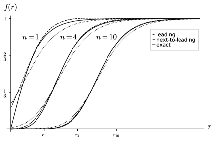
Figure 1: The numerical solution of the exact critical vortex equations for the scalar field $f(r)$ (solid lines), the leading asymptotic boundary layer solution (dotted lines), and the next-to-leading approximation (dashed lines) for different winding numbers $n$.

This equation has a first integral $I=w^{\prime 2}-e^{2w}+2w$ with $I=-1$ corresponding to the boundary condition $w(\infty)=0$. Thus Eq. (6) can be solved in quadratures with the result

$$\begin{split}&\int^{w(x)}_{w_{0}}{{\rm d}w\over(e^{2w}-2w-1)^{1/2}}=x\,,\\ &\gamma(x)=-(e^{2w(x)}-2w(x)-1)^{1\over 2}\,,\end{split}$$ (8)

where $w_{0}=w(0)$ is the second integration constant. It is determined by the boundary condition $w^{\prime}(x)\sim-x$ at $x\to-\infty$, which ensures that Eq. (8) can be matched to the core solution. This gives a new transcendental constant

$$w_{0}=-0.2997174398\ldots\,,$$ (9)

which determines a unique asymptotic solution in the boundary layer. It has a Taylor expansion $w(x)=\sum_{m=0}^{\infty}w_{m}x^{m}$ where $w_{1}=(e^{2w_{0}}-2w_{0}-1)^{1/2}$ and the higher order coefficients can be obtained recursively

$$w_{2}={e^{2w_{0}}-1\over 2}\,,\quad w_{3}={w_{1}\over 3}e^{2w_{0}}\,,\quad w_{4}={w_{1}^{2}+w_{2}\over 6}e^{2w_{0}}\,,\quad\ldots\,.$$ (10)

The asymptotic behavior of the function at $x\to\infty$ reads

$$\begin{split}&w(-x)\sim-{x^{2}\over 2}-{1\over 2}\,,\\ &w(x)\sim w_{\infty}e^{-\sqrt{2}x}\,,\end{split}$$ (11)

where the constant

$$w_{\infty}=w_{0}\exp\left[\int_{w_{0}}^{0}\left({\sqrt{2}\over(e^{2w}-2w-1)^{1/2}}+{1\over w}\right){\rm d}w\right]=-0.331186\ldots\,$$ (12)

is computed in Appendix A. By matching Eq. (11) to the core solution, Eq. (5), in the region $1\ll r_{n}-r\ll r_{n}$ where both approximations are valid we get $F=1/\sqrt{e}$.

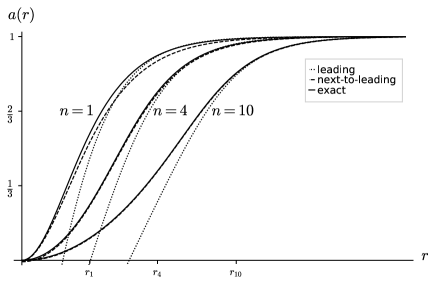
Figure 2: Same as Fig. 1 but for the gauge field $a(r)$.

The vortex tail. For $(r-r_{n})/r_{n}={\cal O}(1)$ the boundary layer approximation breaks down and the coordinate dependence of the field equation coefficients should be restored. However, the deviation of the fields from the vacuum configuration is now exponentially small so the field equations linearize. The solution of the linearized theory is well known and reads

$$\begin{split}&f(r)\sim 1+{\nu\over 2\pi}K_{0}(\sqrt{2}r)+\ldots\,,\\ &a(r)\sim 1+{\mu\over 2\pi}{\sqrt{2}r}K_{1}(\sqrt{2}r)+\ldots\,,\end{split}$$ (13)

where $K_{m}(z)$ is the $m$th modified Bessel function. It describes the field of a point-like source of scalar charge $\nu$ and magnetic dipole moment $\mu$ with $\nu=\mu$ for critical coupling. Eqs. (8) and (13) should coincide in the second matching region $1\ll r-r_{n}\ll r_{n}$, which yields

$$\nu=4w_{\infty}\sqrt{\pi}e^{2\sqrt{n}+\ln(n)/4}\,.$$ (14)

Next-to-leading order solution. For a finite winding number the above asymptotic formulae have a finite accuracy which may deteriorate as $n$ decreases. To get control over the accuracy and convergence of the large-$n$ expansion we compute the ${\cal O}(1/\sqrt{n})$ correction to the asymptotic result. Let us consider first the boundary layer. Writing the corrections to the asymptotic solutions $w$ and $\gamma$ as $\delta w/\sqrt{2n}$ and $\delta\gamma/\sqrt{2n}$, respectively, and expanding Eq. (3) through ${\cal O}(x/r_{n})$ we get the following field equations

$$\begin{split}&\delta w^{\prime\prime}-2e^{2w}\delta w=-w^{\prime}\,,\\ &\delta\gamma(x)=-{x}w^{\prime}(x)-\delta w^{\prime}(x)\,,\end{split}$$ (15)

i.e. $\delta\gamma$ is completely determined by the solution for $\delta w$. The latter obeys the boundary conditions $\delta w(x)\sim x^{3}/6+{\cal O}(1)$ at $x\to-\infty$, $\delta w(\infty)=0$, and can be found in a straightforward though not completely obvious way. By equating the variation of the first integral $I$ to zero and changing the variable from $dx$ to $dw=w^{\prime}dx$ we get the following first-order equation for the homogeneous part of the solution $\delta w^{h}$

$${d\over dw}\left[\left(e^{2w}-2w-1\right)\frac{d\,\delta w^{h}}{dw}-\left(e^{2w}-1\right)\delta w^{h}\right]=0\,.$$ (16)

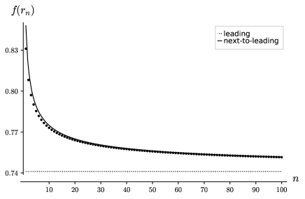
Figure 3: The values $f(r_{n})$ obtained from the numerical solution of the exact critical vortex equations (black dots), the asymptotic value $f(r_{n})=e^{w_{0}}$ (dotted line), and the next-to-leading approximation (solid line) as functions of the winding number $n$.

One solution of this equation is given by the translational zero mode $w^{\prime}(x)$ and we take $w^{\prime}(x)\int_{-\infty}^{x}{\rm d}y/w^{\prime 2}(y)$ as the second solution so that the pair has unit Wronskian. This results in the following solution of Eq. (15) which satisfies the boundary condition at $x\to\infty$

$$\delta w(x)=w^{\prime}(x)\int_{x_{0}}^{x}w^{\prime 2}(y)\int_{-\infty}^{y}\frac{1}{w^{\prime 2}(z)}{\rm d}z{\rm d}y+w^{\prime}(x)\int_{-\infty}^{x}\frac{{\rm d}z}{w^{\prime 2}(z)}\int_{x}^{\infty}w^{\prime 2}(y){\rm d}y\,,$$ (17)

where $x_{0}$ is an integration constant to be determined. A variation of $x_{0}$ changes Eq. (17) by a term proportional to $w^{\prime}(x)$ and therefore does not affect its behavior at $x\to\infty$. For $x_{0}\to\infty$ the two integrals in Eq. (17) can be combined into

$$-w^{\prime}(x)\int_{x}^{\infty}\int_{x}^{y}\frac{w^{\prime 2}(y)}{w^{\prime 2}(z)}{\rm d}z{\rm d}y=-w^{\prime}(x)\int_{x}^{\infty}\int_{z}^{\infty}\frac{w^{\prime 2}(y)}{w^{\prime 2}(z)}{\rm d}y{\rm d}z\,.$$ (18)

The last integral up to a term proportional to $w^{\prime}(x)$ is equal to

$$w^{\prime}(x)\int_{0}^{x}\int_{z}^{\infty}\frac{w^{\prime 2}(y)}{w^{\prime 2}(z)}{\rm d}y{\rm d}z\,.$$ (19)

Thus the next-to-leading contribution can be written as follows

$$\delta w(x)=w^{\prime}(x)\left(C+\int_{0}^{x}\int_{z}^{\infty}{w^{\prime 2}(y)\over w^{\prime 2}(z)}{\rm d}y{\rm d}z\right)\,,$$ (20)

where the integration constant

$$C=\int_{-\infty}^{0}\left({z\over 3}+\int^{\infty}_{z}{w^{\prime 2}(y)\over w^{\prime 2}(z)}{\rm d}y\right)dz=0.529935\ldots\,$$ (21)

is adjusted to satisfy the boundary condition at $x\to-\infty$ (see Appendix A). Eq. (20) determines the next-to-leading approximation in the boundary layer. In the core and tail regions the neglected nonlinear terms are exponentially suppressed and the corrections to the asymptotic result enter only through the matching to the boundary layer solution. To perform the matching we need the asymptotic behavior of Eq. (20) at $|x|\to\infty$ which is computed in Appendix A. For $x\to\infty$ it reads

$$\begin{split}&\delta w(-x)\sim-{x^{3}\over 6}+B\,,\\ &\delta w(x)\sim-w_{\infty}\sqrt{2}{e}^{-\sqrt{2}x}\left(D+\frac{x}{2\sqrt{2}}\right)\,,\end{split}$$ (22)

where

$$B=\int_{-\infty}^{0}\left[{\left(e^{2w}-2w-1\right)^{1\over 2}}-\left(-{2w}\right)^{1\over 2}\left(1+{1\over 4w}\right)\right]{\rm d}w=0.274111\ldots\,,$$ (23)

and

$$D=C+\int_{0}^{\infty}\left(-\frac{1}{2\sqrt{2}}+\int_{z}^{\infty}\frac{w^{\prime 2}(y)}{w^{\prime 2}(z)}{\rm d}y\right){\rm d}z=0.440087\ldots\,.$$ (24)

The first line of Eq. (22) in the matching region $0\ll r_{n}-r\ll r_{n}$ determines the correction to the core solution integration constant

$$F=e^{-{1\over 2}+{B\over\sqrt{2n}}}\,.$$ (25)

Analogously the matching of the second line of Eq. (22) to the tail solution in the region $1\ll r-r_{n}\ll r_{n}$ determines the correction to the scalar charge $\nu$, which we write as $\delta\nu/\sqrt{n}$. Expanding Eq. (13) at large $r$ and keeping the subleading term we get

$$f(r)\sim 1+\frac{\nu+\delta\nu/\sqrt{n}}{2\pi}\left(\frac{\pi}{2\sqrt{2}r}\right)^{1\over 2}e^{-\sqrt{2}r}\left(1-\frac{1}{8\sqrt{2}r}+{\cal O}(1/r^{2})\right)\,.$$ (26)

Further expansion of Eq. (26) with $r=r_{n}+x$ in $x/r_{n}$ and matching to the second line of Eq. (22) gives

$${\delta\nu\over\nu}={1\over 16}-D=-0.377587\ldots\,,$$ (27)

which completes the next-to-leading approximation of the critical vortex solution.

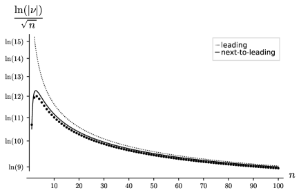
Figure 4: Scalar charge/magnetic dipole moment $\nu$ of a critical vortex obtained from the numerical solution of the exact vortex equations (black dots), the asymptotic result Eq. (14) (dotted line), and the next-to-leading approximation (solid line) as functions of the winding number $n$.

We can now scrutinise the accuracy and convergence of the large-$n$ expansion by comparing the leading and next-to-leading approximations to numerical solutions of the exact field equations for different winding numbers. The results of the analysis for the critical vortices are presented in Figs. 1-4. In Fig. 1 the leading and next-to-leading boundary layer solutions for the scalar field $f(r)$ are plotted against the exact (numerical) solutions with $n=1,\,4,\,10$. Similar plots for the gauge field $a(r)$ are given in Fig. 2. In Figs. 3 and 4 the exact numerical values of $f(r_{n})$ and $\nu$, the natural characteristics of the vortex solution, are plotted against the leading and next-to-leading results for $n=1,\ldots,100$. The expansion reveals an impressive convergence and the next-to-leading approximation works reasonably well even for $n=1$.

2.2 Noncritical vortices

For noncritical scalar self-coupling $\lambda\neq 1$ the order of the field equations cannot be reduced and they read

$$\begin{split}&{1\over r}{d\over dr}\left(r{df\over dr}\right)-\left[\lambda(f^{2}-1)+{n^{2}\over r^{2}}(1-a)^{2}\right]f=0\,,\\ &r{d\over dr}\left({1\over r}{da\over dr}\right)+{2}(1-a)f^{2}=0\,.\end{split}$$ (28)

Nevertheless, the general structure of the solution is quite similar to the critical case. Inside the core the contribution of the scalar potential to Eq. (28) is suppressed by $r^{2}/n^{2}$. Hence the core dynamics is not sensitive to $\lambda$ and the core solution is given by Eq. (5) up to the value of the integration constants which do depend on $\lambda$ through the matching to the non-linear boundary layer solution. In particular the vortex size $r_{n}$ is determined by the region where the two terms in the square brackets of Eq. (28) become comparable and the core approximation breaks down, which gives the leading order result $r_{n}=\sqrt{2n}/\lambda^{1/4}$. Note that the approximately constant energy density in the core is now $\lambda\eta^{2}$ so that the total vortex energy in the large-$n$ limit is $T=2\pi\sqrt{\lambda}n\eta^{2}$. In the tail solution, Eq. (13), the argument of $K_{0}$ gets an additional factor of $\sqrt{\lambda}$ to account for the variation of the scalar field mass, while the scalar charge and the magnetic dipole moment are not equal anymore and have different leading behavior at $n\to\infty$

$$\begin{split}&|\nu|\sim e^{2\sqrt{n}\,\lambda^{1/4}+\ldots}\,,\qquad|\mu|\sim e^{2\sqrt{n}/\lambda^{1/4}+\ldots}\,.\end{split}$$ (29)

More accurately these parameters as well as the normalization of the scalar field in the core solution are determined by matching to the boundary layer solution. In the boundary layer by expanding $r=r_{n}+x$ in $x/r_{n}$ we get a system of $n$-independent equations with constant coefficients

$$\begin{split}&{f^{\prime\prime}}-\left[{\lambda}\left({f^{2}}-1\right)+{\gamma^{2}}\right]f=0\,,\\ &\gamma^{\prime\prime}-{2}\gamma{f^{2}}=0\,,\end{split}$$ (30)

and the boundary conditions $\gamma(x)\sim\sqrt{\lambda}x$ at $x\to-\infty$, $\gamma(\infty)=f(-\infty)=0$, and $f(\infty)=1$. These equations describe a domain wall separating the regions of broken and unbroken symmetry phases in the one-dimensional effective field theory. For $\lambda=1$ the proper solution is given by Eq. (8), and for any given $\lambda\neq 1$ it can be found numerically. The asymptotic profiles of the boundary layer solution with $\lambda=1/2,\,1,\,2$ are plotted in Figs. 5 and 6. In general for $\lambda\neq 1$ the analytic result for the boundary layer solution is out of reach. However, in a number of special limits the boundary layer dynamics vastly simplifies. Below we consider these limits which gives crucial insight into the convergence and accuracy of the large-$n$ expansion for the noncritical case.

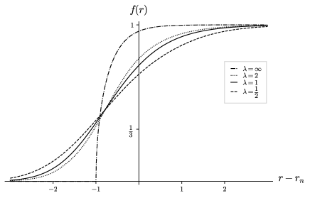
Figure 5: The asymptotic profiles of the scalar field $f(r)$ obtained by numerical solution of the boundary layer equations for different values of scalar self-coupling and the analytic result Eq. (36) for $\lambda\to\infty$ as functions of $r-r_{n}$. For $\lambda\to 0$ the scalar field vanishes throughout the boundary layer as $\lambda^{1/4}$.

Near-critical coupling. For small deviation $\delta\lambda\equiv\lambda-1$ from the critical value an expansion in $\delta\lambda$ about the critical vortex solution can be employed. In particular the corrections in $\delta\lambda$ can be retained only in the leading asymptotic result while the critical coupling result of the previous section can be used for the ${\cal O}(1/\sqrt{n})$ terms. Note that the vortex energy is not proportional to the topological charge anymore and gets a ${\cal O}(\delta\lambda/\sqrt{n})$ contribution which can be easily evaluated. Indeed we can consider the $-\delta\lambda(|\phi|^{2}-\eta^{2})^{2}/2$ term as a perturbation to the critical coupling Lagrangian and get the correction to the vortex energy by evaluating the perturbation on the critical vortex solution. This gives

$$\delta T = {\eta^{2}\delta\lambda\over 2}\int\left(1-f^{2}(r)\right)^{2}{\rm d}^{2}{\mbox{\boldmath$r$}}$$ (31)

$$= {\eta^{2}\delta\lambda\over 2}\left[\int\left(1-f^{2}(r)\right){\rm d}^{2}{\mbox{\boldmath$r$}}-\int\left(1-f^{2}(r)\right)f^{2}(r){\rm d}^{2}{\mbox{\boldmath$r$}}\right]\,.$$

Here the first integral in the brackets is the magnetic flux $2\pi n$ while the second integral is saturated in the boundary layer with an exponential accuracy. Thus in the latter we can approximate the volume element as follows ${\rm d}^{2}{\mbox{\boldmath$r$}}\to 2\pi\sqrt{2n}{\rm d}x=2\pi\sqrt{2n}{\rm d}w/w^{\prime}$ and transform it into $-2\pi\sqrt{n}\sigma$, where

$$\sigma=\int_{-\infty}^{0}{\sqrt{2}(1-e^{2w})e^{2w}\over(e^{2w}-2w-1)^{1/2}}{\rm d}w=0.775304\ldots\,.$$ (32)

The correction to the critical vortex energy then reads

$$\delta T=\pi n\eta^{2}\delta\lambda\left(1-{\sigma\over\sqrt{n}}+{\cal O}(1/n)\right)\,,$$ (33)

where the first term originates from the expansion of the asymptotic result $2\pi\sqrt{\lambda}n\eta^{2}$ in $\delta\lambda$ and the second term represents the correction to the boundary layer energy. Thus the energy of a near-critical giant vortex to the first order in $\delta\lambda$ can be written as follows

$$T=2\pi\sqrt{\lambda}n\eta^{2}\left(1-{\delta\lambda\,\sigma\over 2\sqrt{n}}+{\cal O}(\delta\lambda/n)\right)\,.$$ (34)

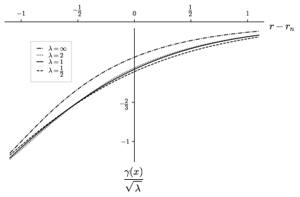
Figure 6: Same as Fig. 5 but for the normalized gauge field $\gamma(x)/\sqrt{\lambda}$.

Large scalar self-coupling. In the limit $\lambda\to\infty$, after a field rescaling $\gamma_{\lambda}(x)=\gamma(x)/\sqrt{\lambda}$ we may neglect the derivative term in the first line of Eq. (30), which becomes algebraic and can be solved for the function $f(r)$. The field equations then become

$$\begin{split}&f^{2}-1+{\gamma_{\lambda}^{2}}=0\,,\\ &\gamma_{\lambda}^{\prime\prime}-2\gamma_{\lambda}+2\gamma_{\lambda}^{3}=0\,.\end{split}$$ (35)

The second line of Eq. (35) has a first integral ${\gamma_{\lambda}^{\prime}}^{2}-2\gamma_{\lambda}^{2}+\gamma_{\lambda}^{4}=0$ corresponding to the boundary value $\gamma_{\lambda}(\infty)=0$. In contrast to Eq. (30) it can be integrated in terms of elementary functions $\gamma_{\lambda}(x)=-\sqrt{2}\,{\rm sech}\left(\sqrt{2}(x-x_{0})\right)$, where $x_{0}$ is the remaining integration constant formally determined by the boundary conditions at $x\to-\infty$. However, for large scalar self-coupling these boundary conditions are rather peculiar since the matching region shrinks to a point $x=0$. Indeed, in the matching region the scalar field is exponentially suppressed $f(r)={\cal O}(e^{-\sqrt{\lambda}x^{2}/2})$ and at $\lambda\to\infty$ it vanishes for all $x<0$ and at $x=0$ its derivative is infinite. At the same time for negative $x$ the gauge field is given by the core solution and has a continuous first derivative at $x=0$. These conditions are satisfied for $x_{0}=-{\rm arcsinh}\left(1\right)/\sqrt{2}$. Thus the boundary layer solution for $x\geq 0$ reads

$$\begin{split}&f(r_{n}+\delta r_{n}+x)=\left(1-{\gamma^{2}(x)\over\lambda}\right)^{1\over 2}\,,\\ &\gamma(x)=-{\sqrt{2\lambda}}\,{\rm sech}\left(\sqrt{2}(x-x_{0})\right)\,,\end{split}$$ (36)

while $f(r)=0$, $a(r)=r^{2}/r_{n}^{2}$ inside the core for $r\leq r_{n}+\delta r_{n}$, where $\delta r_{n}=-1$. Note that now $r=r_{n}+\delta r_{n}+x$, i.e. the core radius which defines the origin of the $x$ coordinate gets a ${\cal O}(\lambda^{1/4}/\sqrt{n})$ correction. This correction makes the winding number of the above gauge field configuration an integer. We can now compute the finite-$n$ correction to the vortex energy. As in the case of near-critical coupling it comes from two sources. Due to the variation of the radius the core energy changes by $-1$ in the units of $2\pi\lambda^{3/4}\sqrt{2n}\eta^{2}$. The contribution of the boundary layer in the same units is ${2\sqrt{2}-1\over 3}$. In total this gives

$$T=2\pi\sqrt{\lambda}n\eta^{2}\left(1-{4(\sqrt{2}-1)\over 3}{\lambda^{1/4}\over\sqrt{n}}+{\cal O}(1/\sqrt{n})\right)\,.$$ (37)

Eq. (37) is consistent with the known negative surface tension on the phase interface in extreme type-II superconductors Thomas . The boundary layer solution, Eq. (36), is subject to enhanced ${\cal O}(\lambda^{1/4}/\sqrt{n})$ corrections which can be obtained in analytic form by the method of Sec. 2.1. It is convenient to write the corrections to $f(r_{n}+\delta r_{n}+x)$ and $\gamma_{\lambda}(x)$ as ${\lambda^{1/4}\over\sqrt{2n}}\delta f(x)$ and ${\lambda^{1/4}\over\sqrt{2n}}\delta\gamma_{\lambda}(y)$, where $y=x-x_{0}$. Then for the gauge field we get (see Appendix B)

$$\delta\gamma_{\lambda}(y) = {e^{-\sqrt{2}y}\over 6}\left(1+e^{2\sqrt{2}y}\right)^{-2}\left[1+\left(4+10\sqrt{2}-18\sqrt{2}(y+x_{0})\right)e^{2\sqrt{2}y}\right.$$ (38)

$$+ \left.\left(-13+14\sqrt{2}-6\sqrt{2}(y+x_{0})\right)e^{4\sqrt{2}y}\right]\,,$$

and the result for the scalar field is obtained by substituting Eq. (38) into the first line of Eq. (67).

Small scalar self-coupling. In the limit $\lambda\to 0$ the light scalar field extends beyond the core radius $r_{n}$ and up to the scale $x_{\lambda}\equiv\sqrt{2/\lambda}$. In this region the gauge field can be neglected and the first line of Eq. (30) becomes

$$\begin{split}&{f^{\prime\prime}}+\lambda\left(f-f^{3}\right)=0\,.\end{split}$$ (39)

It has a first integral ${f^{\prime}}^{2}-(\lambda/2)(1-f^{2})^{2}=0$ corresponding to the boundary value $f(\infty)=1$ and a “half-kink” solution

$$\begin{split}&f(r_{n}+x)={\rm tanh}\left(x/x_{\lambda}\right)\,.\end{split}$$ (40)

Inside the boundary layer the scalar self-coupling can be neglected in the field equations. However, the boundary conditions for the corresponding solution do depend on $\lambda$. As before matching to the core requires $\gamma(x)\sim\sqrt{\lambda}x$ at $x\to-\infty$ while matching to the half-kink solution Eq. (40) gives $f(r_{n}+x)\sim\sqrt{\lambda/2}x$ at $1\ll x\ll x_{\lambda}$. This dependence can be eliminated by a rescaling

$$z=\lambda^{1/4}x\,,\quad\gamma_{\lambda}(z)={\gamma(x)\over\lambda^{1/4}}\,,\quad f_{\lambda}(z)={\sqrt{2}\over\lambda^{1/4}}f(r_{n}+x)\,.$$ (41)

In the new variables the boundary layer equations read

$$\begin{split}&{f^{\prime\prime}_{\lambda}}-\gamma_{\lambda}^{2}f_{\lambda}=0\,,\\ &\gamma_{\lambda}^{\prime\prime}-f_{\lambda}^{2}\gamma_{\lambda}=0\,,\end{split}$$ (42)

with the boundary conditions $\gamma_{\lambda}(z)\sim z$, $f_{\lambda}(z)={\cal O}(e^{-z^{2}/2})$ at $z\to-\infty$ and $f_{\lambda}(z)\sim z$, $\gamma_{\lambda}(z)={\cal O}(e^{-z^{2}/2})$ at $z\to\infty$. The above system is invariant with respect to the discrete field transformations $f_{\lambda}\to-f_{\lambda}$, $\gamma_{\lambda}\to-\gamma_{\lambda}$, and $f_{\lambda}\leftrightarrow\gamma_{\lambda}$, as well as the coordinate reflection $z\to-z$. Taking into account the boundary conditions we find that the gauge and the scalar fields have “mirror” boundary layer solutions

$$\gamma_{\lambda}(z)=-f_{\lambda}(-z)\,.$$ (43)

Despite the high symmery and the existence of a first integral ${\gamma_{\lambda}^{\prime}}^{2}+{f_{\lambda}^{\prime}}^{2}-\gamma_{\lambda}^{2}f_{\lambda}^{2}=1$ Eq. (42) cannot be integrated in quadratures, at least not in a straightforward way. However, we can conclude that inside the boundary layer of width $1/\lambda^{1/4}$ the gauge and scalar fields scale as $\lambda^{1/4}$, and hence the boundary layer contributes a plain ${\cal O}(1/\sqrt{n})$ correction to the vortex energy. Thus the total correction to the energy is dominated by the scalar cloud outside the boundary layer, Eq. (40), which gives

$$T=2\pi\sqrt{\lambda}n\eta^{2}\left(1+{4\over 3\lambda^{1/4}\sqrt{n}}+{\cal O}(1/\sqrt{n})\right)\,.$$ (44)

Eq. (44) agrees with a classical result for the positive surface tension in extreme type-I superconductors Landau . The scalar cloud solution itself gets the enhanced finite-$n$ correction. It can be written as $\delta f(y)/{(\sqrt{2n}\lambda^{1/4})}$, where $y=x/x_{\lambda}$ and

$$\delta f(y)={9+12y-8e^{-2y}-e^{-4y}\over 6\sqrt{2}(2+e^{2y}+e^{-2y})}\,.$$ (45)

The details of the derivation of this result are presented in Appendix B.

We should emphasize that the accuracy and convergence of the large-$n$ expansion for noncritical vortices crucially depend on the scale of $\lambda$, cf. Eqs. (37, 44). For large scalar self-coupling the expansion clearly breaks down at $n={\cal O}(\sqrt{\lambda})$ where the ratio of scales characterizing the boundary layer and the core dynamics $\delta r_{n}/r_{n}$ is not small anymore. At this value the dependence on the winding number qualitatively changes. Indeed, in the limit $\lambda\to\infty$ with fixed $n$ we should recover the classical result Abrikosov:1956sx ; Landau where the scalar field core radius vanishes as $n/\sqrt{\lambda}$, a characteristic size of the gauge field core is ${\cal O}(1)$, and the energy is quadratic in the magnetic flux and logarithmic in the scalar coupling constant

$$T\sim 2\pi n^{2}\eta^{2}\ln(\sqrt{\lambda}/n)\,.$$ (46)

For small $\lambda$ the convergence problem appears at $n={\cal O}(1/\sqrt{\lambda})$. For such $n$ the expansion in the ratio $x_{\lambda}/r_{n}$ of the scales characterizing the dynamics of the scalar cloud and the vortex core breaks down, and the structure of the solution is no longer described by the asymptotic formulae. In particular, in the limit $\lambda\to 0$ at fixed $n$ the vortex energy is dominated by the scalar cloud contribution, which can depend on the scalar self-coupling and the winding number at most logarithmically.

3 Ginzburg-Pitaevskii vortices

The Ginzburg-Pitaevskii vortex equation Ginzburg:1958 for a neutral complex scalar field $\phi$ which describes a Bose-Einstein condensate of weakly interacting Bose gas can be obtained from the analysis of the previous section by setting the gauge field to zero and rescaling the scalar self-coupling to $\lambda=1$. The corresponding radial equation reads

$${1\over r}{d\over dr}\left(r{df\over dr}\right)+\left(1-{n^{2}\over r^{2}}-f^{2}\right)f=0\,.$$ (47)

The structure of its solution in the limit of large $n$ is quite distinct from the Abrikosov-Nielsen-Olesen case discussed above. Now the field dynamics is essentially different in the vortex core $r\ll r_{n}$, its tail $r\gg r_{n}$, and in the matching region around $r=r_{n}$, where $r_{n}=n$ gives the leading approximation for the size of the region with unbroken symmetry phase. Let us consider the field dynamics and the vortex solution in each region.

The vortex core. For $r\ll r_{n}$ the solution $f(r)\propto r^{n}$ is exponentially suppressed with $n$ so that the nonlinear cubic term can be neglected. As $r$ approaches $r_{n}$ the ${\cal O}(1)$ linear term in the equation becomes relevant while the exponentially suppressed nonlinear term can still be omitted and we get a linear differential equation

$${1\over r}{d\over dr}\left(r{df\over dr}\right)+\left(1-{n^{2}\over r^{2}}\right)f=0\,,$$ (48)

with the regular solution proportional to the $n$th Bessel function $J_{n}(r)$. Since $J^{(m)}_{n}(n)={\cal O}(1/n^{m+1\over 3})$, near $r=r_{n}$ all the terms of Eq. (48) are ${\cal O}(1/n)$ and the nonlinear part cannot be neglected. To estimate the maximal $r$ where Eq. (48) is still valid we use an asymptotic formula

$$J_{n}(r_{n}+x)\sim\left(2\over n\right)^{1\over 3}{\rm Ai}(-z)\left(1+{\cal O}(z/n^{2/3})\right)\,,$$ (49)

where ${\rm Ai}(z)$ is the Airy function, $x=r-r_{n}$, and $z=(2/n)^{1/3}x$. The Airy function is exponentially suppressed for large positive values of the argument, hence the core approximation is valid for $r_{n}-r\;\hbox to0.0pt{\lower 3.5pt\hbox{$\mathchar 0\relax\sim$}\hss}\raise 1.0pt\hbox{$>$}\;n^{1/3}$.

The vortex tail. In the opposite limit $r\gg r_{n}$ the derivative term in the equation is suppressed and can be treated as a perturbation. As a result the field equation becomes algebraic. For example, in the leading order we get

$$f^{2}-1+{n^{2}\over r^{2}}=0\,,$$ (50)

with the solution

$$f(r)=\left(1-{n^{2}\over r^{2}}\right)^{1\over 2}\,.$$ (51)

The higher order terms can easily be obtained by iterations to any desired order in $1/r$. The first three terms read

$$f(r) = \left(1-{n^{2}\over r^{2}}\right)^{1\over 2}-{n^{2}\over r^{4}}\left(1-{n^{2}\over 2r^{2}}\right)\left(1-{n^{2}\over r^{2}}\right)^{-{5\over 2}}$$ (52)

$$+ {n^{2}\over r^{6}}\left(8+{3n^{2}\over 2r^{2}}-{n^{4}\over 2r^{4}}+{n^{6}\over 8r^{6}}\right)\left(1-{n^{2}\over r^{2}}\right)^{-{11\over 2}}+{\cal O}(1/r^{8})\,.$$

The expansion Eq. (52) formally breaks down for $x={\cal O}(n^{1/3})$. Indeed, let us consider the behavior of the above series at $x={\kappa}^{1-\alpha}n^{\alpha}/2$ for some power $\alpha$. Here the factor ${\kappa}^{1-\alpha}/2$ with a constant $\kappa$ is introduced for convenience. Then the series Eq.(52) can be written as an expansion

$$f(r)=\left({\kappa\over n}\right)^{1-\alpha\over 2}\sum_{m=1}^{\infty}f_{m}\rho^{m}\,,$$ (53)

where $\rho={\kappa^{3\alpha-3}/n^{3\alpha-1}}$. Each $f_{m}$ can in turn be expanded in $\tau=(\kappa/n)^{1-\alpha}$. For the first three terms we get

$$f_{1}=1-{3\over 8}\tau+{23\over 128}\tau^{2}+\ldots\,,$$

$$f_{2}={1\over 2}+{7\over 16}\tau-{117\over 256}\tau^{2}+\ldots\,,$$ (54)

$$f_{3}={73\over 8}+{601\over 64}\tau+{1215\over 1024}\tau^{2}+\ldots\,.$$

For $\alpha\leq 1/3$ the expansion parameter $\rho$ is not suppressed at large $n$ and the series Eq. (52) is not defined (though for the boundary case $\alpha=1/3$ we have $\rho=1/\kappa^{2}$ and the series may converge for sufficiently large $\kappa$). At the same time the expansion parameter $\tau$ is not suppressed for $\alpha\geq 1$. Thus the allowed interval for the expansion in negative powers of $n$ is $1/3<\alpha<1$. For $\alpha=1/2$ both expansions in $\rho$ and $\tau$ convert into a series in $1/\sqrt{n}$. Note that by choosing a smaller or larger value of $\alpha$ we boost the convergence of the expansion in $\tau$ or $\rho$, respectively, and for a given $\alpha$ the parameter $\kappa$ can be tuned to further improve the convergence of the series.

The matching region. The problem now is to derive a large-$n$ expansion in the matching region $-n^{1/3}\;\hbox to0.0pt{\lower 3.5pt\hbox{$\mathchar 0\relax\sim$}\hss}\raise 1.0pt\hbox{$<$}\;x\;\hbox to0.0pt{\lower 3.5pt\hbox{$\mathchar 0\relax\sim$}\hss}\raise 1.0pt\hbox{$<$}\;n^{\alpha}$. First we note that in this interval the solution is suppressed at least as $1/n^{5\alpha-1\over 2}$, i.e. at $n\to\infty$ the boundary layer does not develop. Moreover, the core solution at $x={\cal O}(1)$ and the tail solution at $x={\cal O}(n^{1/3})$ have the property $f^{(m)}(r)={\cal O}(1/n^{m+1\over 3})$, which means that they can be polynomially matched over the corresponding interval. A linear matching of the leading core and tail solutions gives a simple analytic formula Penin:2020cxj

$$f(r)=\left\{\begin{array}[]{l}C^{\prime}J_{n}(r)\,,\quad r\leq r_{n}\,,\\[3.0pt] (\delta/2n)^{1/2}\left(1+{(r-r_{n})/\delta}\right),\,r_{n}<r<r_{n}+\delta\,,\\[3.0pt] \left(1-{n^{2}/r^{2}}\right)^{1/2}\,,\quad r_{n}+\delta\leq r\,,\end{array}\right.$$ (55)

where $C^{\prime}={3^{1/4}\pi^{1/2}\over 2^{1/2}}$, $\delta/n^{1/3}={2^{2/3}\pi\over 3^{5/6}\Gamma^{2}(2/3)}$, and $\Gamma(z)$ is the Euler gamma-function. In the limit $n\to\infty$ the function defined by Eq. (55) becomes continuous and smooth. As has been discussed above, the higher orders of the perturbative expansion of the core solution in the nonlinear term at $x={\cal O}(1)$ as well as the perturbative expansion of the tail solution in the derivative term at $x={\cal O}(n^{1/3})$ are not suppressed by extra powers of $n$ (though both expansion may de facto converge). Thus Eq. (55) gives the asymptotic solution up to ${\cal O}(1/n^{1/3})$ corrections. It can be used to obtain the analytic result for the vortex energy at $n\to\infty$. The total energy consists of the logarithmically divergent rotational part $T_{rot}$ and the nonrotational finite part $T$ Ginzburg:1958 . The rotational contribution determined by the angular part of the kinetic term reads

$$T_{rot}=\eta^{2}\int{|\partial_{\theta}\phi({\mbox{\boldmath$r$}})/r|^{2}}{\rm d}^{2}{\mbox{\boldmath$r$}}\approx 2\pi n^{2}\eta^{2}\left(\ln\left({R/r_{n}}\right)-{1\over 2}\right)\,,$$ (56)

where $R\gg r_{n}$ is the radial integration cutoff (the physical radius of rotating condensate). For the remaining part saturated by the field potential we get $T=\pi n^{2}\eta^{2}$, where a half of the contribution comes from the vortex tail. As expected the logarithmic term in Eq. (56) agrees with Eq. (46) upon identification of $R$ with the characteristic size of the gauge field core and $r_{n}$ with the one of the scalar core.

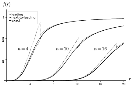
Figure 7: The numerical solution of the exact vortex equations for a neutral scalar field $f(r)$ (solid line), the leading asymptotic solution Eq. (55) (dotted line), and the next-to-leading approximation (dashed line) for different $n$.

To obtain the solution at ${\cal O}(1/n^{1/3})$ and beyond, the coefficients of the vortex equation in the matching region are expanded in $x/r_{n}$. Defining

$$f(r)={2^{5/6}\over n^{1/3}}\,\chi\left(-z\right)\,,$$ (57)

we get the leading order $n$-independent nonlinear equation for the function $\chi(z)$

$${d^{2}\chi\over dz^{2}}-z\chi-2\chi^{3}=0\,.$$ (58)

Eq. (58) is a special case of the Painlevé II transcendent. It is known to have a solution $\chi_{0}(z)$ with the following asymptotic behavior at $z\to\infty$ Hastings:1980

$$\begin{split}&\chi_{0}(-z)\sim\left({z\over 2}\right)^{1\over 2}\,,\\ &\chi_{0}(z)\sim{\rm Ai}(z)\,.\end{split}$$ (59)

The corresponding function $f(r)$ matches the core solution $\sqrt{2}J_{n}(r)$ at negative $x={\cal O}(n^{1/3})$ and the leading order tail solution $f_{1}$ at positive $x={\cal O}(\sqrt{n})$. In the next-to-leading order the equation for $\chi(z)$ becomes

$${d^{2}\chi\over dz^{2}}-{1\over 2^{1/3}n^{2/3}}{d\chi\over dz}-z\left(1+{3\over 2^{4/3}}{z\over n^{2/3}}\right)\chi-2\chi^{3}=0\,.$$ (60)

The relevant solution must exponentially decay at $z\to\infty$ and match the expansion of the next-to-leading tail solution $f(r_{n}+x)$ at $x=\sqrt{\kappa n}/2$ through ${\cal O}(1/n)$. It can only be found numerically. Note that since the expansion parameter $x/n$ varies from $1/n$ to $1/\sqrt{n}$ through the matching region, the convergence of the series there is not uniform. In general the expansion of the tail solution in $\rho$ matches the asymptotic expansion of $\chi_{0}(z)$ at large negative $z$ while the series in $\tau$ for each $f_{m}$ is connected with the corrections to the equation for $\chi(z)$.

The results of numerical analysis for the neutral scalar field vortices with $n=4,\,10,\,16$ are presented in Fig. 7. For the leading order approximation the linear matching is used and in the next-to-leading order the numerical solution of Eq. (60) is matched to the first two terms of Eq. (52) at $r_{n}+\sqrt{n/2}$, which corresponds to $\kappa=2$.

4 Summary

We have elaborated a method of expansion in inverse powers of a topological quantum number. The method is quite general and can be applied to the study of topological solitons in a theory where the corresponding quantum number is associated with a ratio of dynamical scales. When applied to axially symmetric vortices with large winding number $n$ the expansion is in negative noninteger powers of $n$ and in general is not uniform. In the large-$n$ limit the complex nonlinear vortex dynamics unravels. In particular, for the Abrikosov-Nielsen-Olesen vortices at critical coupling and in the limit of large or small scalar self-coupling the field equations become integrable. At the same time for the Ginzburg-Pitaevskii vortices in a weakly interacting Bose-Einstein condensate the field equation reduces to an algebraic one. The method yields simple asymptotic formulae for the shape and parameters capturing the main features of the giant vortices. The accuracy of the asymptotic result can be systematically improved by calculating the finite-$n$ corrections. For near-critical vortices the approximation works remarkably well all the way down to very low $n$ after including the leading ${\cal O}(1/\sqrt{n})$ corrections. In the case of extremely small or large scalar self-coupling $\lambda$ the large-$n$ expansion converges and gives a reliable approximation for all winding numbers satisfying the condition $n\gg\sqrt{\lambda},~{}1/\sqrt{\lambda}$.

Acknowledgement
A.P. is grateful to Valery Rubakov for a discussion of noncritical vortices. The work of A.P. was supported in part by NSERC and the Perimeter Institute for Theoretical Physics. The work of Q.W. was supported through the NSERC USRA program.

Appendix A Calculation of the critical vortex parameters

Calculation of ${w_{\infty}}$. The integral in Eq. (8) is logarithmically divergent at $w(x)\to 0$ and can be decomposed as follows

$$\int_{w_{0}}^{w(x)}\frac{{\rm d}w}{(e^{2w}-2w-1)^{1/2}} = -\int_{w_{0}}^{w(x)}\frac{{\rm d}w}{\sqrt{2}w}+\int_{0}^{w(x)}\left(\frac{1}{(e^{2w}-2w-1)^{1/2}}+\frac{1}{\sqrt{2}w}\right){\rm d}w$$ (61)

$$+ \int_{w_{0}}^{0}\left(\frac{1}{(e^{2w}-2w-1)^{1/2}}+\frac{1}{\sqrt{2}w}\right){\rm d}w\,,$$

where the first term is divergent, the second term is ${\cal O}(w(x))$, and the last term is a constant which we denote as $\ln({w_{\infty}/w_{0}})/\sqrt{2}$. Thus Eq. (8) at $w(x)\to 0$ becomes

$$x=-{1\over\sqrt{2}}\ln\left({w(x)\over w_{\infty}}\right)+{\cal O}(w(x))\,,$$ (62)

which after exponentiation gives the second line of Eq. (11).

Calculation of $B$ and $C$. By changing the integration variable $w^{\prime}{\rm d}y={\rm d}w$ the integral in Eq. (20) can be transformed as follows

$$\int_{z}^{\infty}w^{\prime 2}(y){\rm d}y = -\left(-{w(z)\over 2}\right)^{1\over 2}\left(1+{4\over 3}w(z)\right)$$ (63)

$$+ \int_{w(z)}^{0}\left[{\left(e^{2w}-2w-1\right)^{1\over 2}}-\left(-{2w}\right)^{1\over 2}\left(1+{1\over 4w}\right)\right]{\rm d}w\,.$$

At $z\to-\infty$ up to ${\cal O}(1/z)$ corrections the first term is just $-z^{3}/3$ and the second term is a constant which we denote as $B$. This gives

$$\int_{z}^{\infty}{w^{\prime 2}(y)\over w^{\prime 2}(z)}{\rm d}y\sim-\frac{z}{3}+{B\over z^{2}}+\ldots\,,$$ (64)

where the ellipsis stands for the exponentially suppressed terms. Then the integral in Eq. (20) can be decomposed as follows

$$\int_{0}^{x}\int_{z}^{\infty}\frac{w^{\prime 2}(y)}{w^{\prime 2}(z)}{\rm d}y{\rm d}z = -\frac{x^{2}}{6}+\int_{-\infty}^{x}\left(\frac{z}{3}+\int_{z}^{\infty}\frac{w^{\prime 2}(y)}{w^{\prime 2}(z)}{\rm d}y\right){\rm d}z$$ (65)

$$- \int^{0}_{-\infty}\left(\frac{z}{3}+\int_{z}^{\infty}\frac{w^{\prime 2}(y)}{w^{\prime 2}(z)}{\rm d}y\right){\rm d}z\,,$$

where the second term vanishes at $x\to-\infty$ as $-B/x$ and the last term is a constant which has to be cancelled by $C$ in Eq. (20) to provide the correct asymptotic behavior, Eq. (22).

Calculation of $D$. The asymptotic behavior of the integral in Eq. (20) at $x\to\infty$ can be computed via the following decomposition

$$\int_{0}^{x}\int_{z}^{\infty}\frac{w^{\prime 2}(y)}{w^{\prime 2}(z)}{\rm d}y\,{\rm d}z = \frac{x}{2\sqrt{2}}-\int^{\infty}_{x}\left(-\frac{1}{2\sqrt{2}}+\int_{z}^{\infty}\frac{w^{\prime 2}(y)}{w^{\prime 2}(z)}{\rm d}y\right){\rm d}z$$ (66)

$$+ \int_{0}^{\infty}\left(-\frac{1}{2\sqrt{2}}+\int_{z}^{\infty}\frac{w^{\prime 2}(y)}{w^{\prime 2}(z)}{\rm d}y\right){\rm d}z\,,$$

where the second term vanishes at $x\to\infty$ and the last term is a constant. By substituting Eq. (66) into Eq. (20) at $x\to\infty$ we obtain the second line of Eq. (22).

Appendix B Finite-$n$ corrections to the noncritical vortex solution

Large scalar self-coupling. By expanding Eq. (28) about $r_{n}+\delta r_{n}$ we get

$$\begin{split}&\delta f=(1-\gamma_{\lambda}^{2})^{-{1\over 2}}\gamma_{\lambda}\left[(x-1)\gamma_{\lambda}-\delta\gamma_{\lambda}\right]\,,\\ &\delta\gamma_{\lambda}^{\prime\prime}-2\left(1-3\gamma_{\lambda}^{2}\right)\delta\gamma_{\lambda}=\gamma_{\lambda}^{\prime}+4(x-1)\gamma_{\lambda}^{3}\,,\end{split}$$ (67)

which defines an inhomogeneous differential equation on the function $\delta\gamma_{\lambda}(y)$, where $y=x-x_{0}$. The boundary conditions for this equation are $\delta\gamma_{\lambda}(\infty)=0$ and $\delta\gamma_{\lambda}(-x_{0})=1/2$, where the latter is determined by matching to the core solution for the gauge field at $r_{n}+\delta r_{n}$. Note that $\delta f$ and $\delta\gamma_{\lambda}^{\prime\prime}$ are not continuous at this point due to the singular character of the matching region in the limit $\lambda\to\infty$ discussed previously. Due to the existence of the first integral for Eq. (35) the homogeneous part of the solution $\delta\gamma^{h}_{\lambda}$ satisfies the first-order equation

$${d\over d\gamma_{\lambda}}\left[\gamma_{\lambda}^{2}\left(2-\gamma_{\lambda}^{2}\right){d\delta\gamma^{h}_{\lambda}\over d\gamma_{\lambda}}-2\gamma_{\lambda}\left(1-\gamma_{\lambda}^{2}\right)\delta\gamma^{h}_{\lambda}\right]=0\,.$$ (68)

One of its solutions is given by the translational zero mode $\gamma_{\lambda}^{\prime}(y)=2\,{\rm sech}(\sqrt{2}y)\,{\rm tanh}(\sqrt{2}y)$. The second solution reads

$$\delta\gamma^{h}_{\lambda}(y)={{\rm sech}(\sqrt{2}y)\,{\rm tanh}(\sqrt{2}y)\over 8\sqrt{2}}\left(6\sqrt{2}y-4\,{\rm coth}(\sqrt{2}y)+{\rm sinh}(2\sqrt{2}y)\right)\,.$$ (69)

With the solutions of the homogeneous equation at hand, the solution of the full equation is straightforward and gives Eq. (38).

Small scalar self-coupling. The expansion of Eq. (28) with $a(r)=1$ about $r_{n}+\delta r_{n}$ yields

$$\delta f^{\prime\prime}+2(1-3f^{2})\delta f=-\sqrt{2}f^{\prime}\,,$$ (70)

with the boundary conditions $\delta f(\infty)=0$ and $\delta f(0)=0$. The condition at $y=0$ is determined by matching to the boundary layer solution at $x={\cal O}(1/\lambda^{1/4})$. The homogeneous part of the solution satisfies the first-order equation

$${d\over df}\left[{\left(1-f^{2}\right)^{2}\over 2}{d\delta f^{h}\over df}+f\left(1-f^{2}\right)\delta f^{h}\right]=0\,.$$ (71)

It has the translational zero mode $f^{\prime}(y)={\rm sech}^{2}(y)$ and the second solution

$$\delta f^{h}(y)={{\rm sech}^{2}(y)\over 16}\left(12y+8\,{\rm sinh}(2y)+\,{\rm sinh}(4y)\right)\,,$$ (72)

which after straightforward calculation gives Eq. (45).

References

- (1) A. A. Penin and Q. Weller, Phys. Rev. Lett. 125, 251601 (2020).
- (2) A. A. Abrikosov, Sov. Phys. JETP 5, 1174 (1957) [Zh. Eksp. Teor. Fiz. 32, 1442 (1957)].
- (3) V. L. Ginzburg and L. P. Pitaevskii, Sov. Phys. JETP 7, 858 (1958), [Zh. Eksp. Teor. Fiz. 34, 1240 (1958).]
- (4) H. B. Nielsen and P. Olesen, Nucl. Phys. B 61, 45 (1973).
- (5) M. B. Hindmarsh and T. W. B. Kibble, Rept. Prog. Phys. 58, 477 (1995).
- (6) A. A. Penin, V. A. Rubakov, P. G. Tinyakov and S. V. Troitsky, Phys. Lett. B 389, 13 (1996).
- (7) D. Tong, “TASI lectures on solitons: Instantons, monopoles, vortices and kinks,” [arXiv:hep-th/0509216 [hep-th]].
- (8) P. L. Marston, W. M. Fairbank, Phys. Rev. Lett. 39, 1208 (1977).
- (9) P. Engels, I. Coddington, P. C. Haljan, V. Schweikhard, and E. A. Cornell, Phys. Rev. Lett. 90, 170405 (2003).
- (10) T. Cren, L. Serrier-Garcia, F. Debontridder, and D. Roditchev, Phys. Rev. Lett. 107, 097202 (2011).
- (11) E. B. Bogomolny, Sov. J. Nucl. Phys. 24, 449 (1976) [Yad. Fiz. 24, 861 (1976)].
- (12) H. J. de Vega and F. A. Schaposnik, Phys. Rev. D 14, 1100 (1976).
- (13) M. K. Prasad and C. M. Sommerfield, Phys. Rev. Lett. 35, 760 (1975).
- (14) E. Witten, Phys. Rev. Lett. 38, 121 (1977).
- (15) M. K. Prasad and P. Rossi, Phys. Rev. Lett. 46, 806 (1981).
- (16) S. Bolognesi, Nucl. Phys. B 730, 127 (2005).
- (17) S. Bolognesi and S. B. Gudnason, Nucl. Phys. B 741, 1 (2006).
- (18) D. Saint-James, G. Sarma, E. J. Thomas, Type- II Superconductivity, Pergamon Press, Oxford, 1969.
- (19) E. M. Lifshitz, L. P. Pitaevskii, Statistical Physics, Part 2: Theory of the Condensed State, Vol. 9 (1st ed.), Butterworth-Heinemann, Oxford, 1980.
- (20) S. P. Hastings and J. B. McLeod, Arch. Rational Mech. Anal. 73, 31 (1980).