Implications of Increased Central Mass Surface Densities for the Quenching of Low-mass Galaxies

Abstract

We use the Cosmic Assembly Deep Near-infrared Extragalactic Legacy Survey (CANDELS) data to study the relationship between quenching and the stellar mass surface density within the central radius of 1 kpc ($\Sigma_{1}$) of low-mass galaxies (stellar mass $M_{*}\lesssim 10^{9.5}M_{\odot}$) at $0.5\leq z<1.5$. Our sample is mass complete down to $\sim 10^{9}$${\rm\,M_{\odot}}$ at $0.5\leq z<1.0$. We compare the mean $\Sigma_{1}$ of star-forming galaxies (SFGs) and quenched galaxies (QGs) at the same redshift and ${\rm M_{*}}$. We find that low-mass QGs have higher $\Sigma_{1}$ than low-mass SFGs, similar to galaxies above $10^{10}M_{\odot}$. The difference of $\Sigma_{1}$ between QGs and SFGs increases slightly with ${\rm M_{*}}$ at $M_{*}\lesssim 10^{10}M_{\odot}$ and decreases with ${\rm M_{*}}$ at $M_{*}\gtrsim 10^{10}M_{\odot}$. The turnover mass is consistent with the mass where quenching mechanisms transition from internal to environmental quenching. At $0.5\leq z<1.0$, we find that the $\Sigma_{1}$ of galaxies increases by about 0.25 dex in the green valley (i.e., transitioning region from star forming to fully quenched), regardless of their ${\rm M_{*}}$. Using the observed specific star formation rate (sSFR) gradient in the literature as a constraint, we estimate that the quenching timescale (i.e., time spent in the transition) of low-mass galaxies is a few ($\sim 4$) Gyrs at $0.5\leq z<1.0$. The responsible quenching mechanisms need to gradually quench star formation in an outside-in way, i.e., preferentially ceasing star formation in outskirts of galaxies while maintaining their central star formation to increase $\Sigma_{1}$. An interesting and intriguing result is the similarity of the growth of $\Sigma_{1}$ in the green valley between low-mass and massive galaxies, which suggests that the role of internal processes in quenching low-mass galaxies is a question worthy of further investigation.

1. Introduction

Processes of quenching star formation in galaxies can be divided into two categories: internal and external. The latter, or environmental quenching, is believed to be the primary mechanism of quenching galaxies with stellar masses (${\rm M_{*}}$) lower than $10^{9.5}$${\rm\,M_{\odot}}$ (or low-mass galaxies). Evidence of it has been obtained at various cosmic epochs (e.g., Peng et al., 2010, 2012; Geha et al., 2012; Wetzel et al., 2013; Wheeler et al., 2014; Fillingham et al., 2015; Lee et al., 2015; Balogh et al., 2016; Fossati et al., 2017; Guo et al., 2017; Kawinwanichakij et al., 2017; Woo et al., 2017; Ji et al., 2018; Papovich et al., 2018). Peng et al. (2010) showed that environmental and internal (mass) quenching is separable in the local universe and the importance of environmental (plus merger) quenching overtakes that of mass (internal) quenching around $10^{10}$${\rm\,M_{\odot}}$. Guo et al. (2017) used the projected distance ($d_{proj}$) of a galaxy to its nearest massive neighbor with ${\rm M_{*}}$$>10^{10.5}$${\rm\,M_{\odot}}$ as the indicator of environmental quenching and found that low-mass quenched galaxies (QGs) have systematically smaller $d_{proj}$ than star-forming galaxies (SFGs), consistent with the scenario that if environmental effects are significantly responsible for quenching low-mass galaxies, QGs should live preferentially within a massive dark matter halo and hence close to a massive central galaxy. A question, however, remains to be more thoroughly studied: what is the role that internal processes play in the quenching of low-mass galaxies?

To answer this question, an effective indicator of internal processes is needed. Studies of massive galaxies suggest that central mass surface density within the central radius of 1 kpc ($\Sigma_{1}$) is such an indicator. Cheung et al. (2012) found that high $\Sigma_{1}$ is the best predictor of quenching at $z\sim 0.7$. Fang et al. (2013) found that for nearby SDSS galaxies, specific star formation rate (sSFR) varies systematically relative to $\Sigma_{1}$, suggesting a mass-dependent threshold of $\Sigma_{1}$ for the onset of quenching, possibly due to a threshold in black hole mass. van Dokkum et al. (2014), Tacchella et al. (2015), and Barro et al. (2017) extended the use of $\Sigma_{1}$ as a quenching indicator to higher redshifts. Since massive galaxies are primarily quenched by internal processes (e.g. Darvish et al., 2015, 2016; Lin et al., 2016; De Lucia et al., 2019), $\Sigma_{1}$ hence can be treated as an indicator of internal quenching. Moreover, Terrazas et al. (2016) found that quiescence is strongly correlated with black hole mass in central galaxies, suggesting that $\Sigma_{1}$ is very likely a proxy of black hole mass. Chen et al. (2020) proposed a model to correlate $\Sigma_{1}$ with the mass of supermassive black holes. Recently, Luo et al. (2020) correlated $\Sigma_{1}$ with the bulge types in nearby galaxies.

In this paper, we use $\Sigma_{1}$ to explore quenching in low-mass galaxies. Comparing the $\Sigma_{1}$ of QGs and SFGs would reveal clues on the quenching mechanisms. Woo et al. (2017) studied the $\Sigma_{1}$ between SFGs and QGs in SDSS galaxies, and found that in all environments, at a given ${\rm M_{*}}$, QGs have a 0.2-0.3 dex higher $\Sigma_{1}$ than SFGs. They argued that either $\Sigma_{1}$ increases subsequent to satellite quenching, or the $\Sigma_{1}$ for individual galaxies remains unchanged, but the ${\rm M_{*}}$ of galaxies at the time of quenching is significantly different from those in the green valley. Their sample is down to ${\rm M_{*}}$=$10^{9.75}$${\rm\,M_{\odot}}$, just around the ${\rm M_{*}}$, where the quenching mechanisms are believed to change. Currently, however, similar studies are lacking for low-mass galaxies beyond the local universe. We will use the CANDELS data to explore lower-mass regime at $z\geq 0.5$.

The physical meaning of $\Sigma_{1}$ in low-mass and massive galaxies, however, is different. The choice of 1 kpc, which is limited by the spatial resolution of HST/WFC3, is reasonably small for massive galaxies to sample their central region, but it is quite close to the effective radius of low-mass galaxies, raising a concern of its validity to represent the central region. Galaxies, however, extend well beyond their half-light radius. Mowla et al. (2019) showed that the 80%-light radius ($r_{80}$, i.e., the radius containing 80% of the total galaxy light) of low-mass galaxies at $z\lesssim 1.5$ is about 5 kpc, and this radius increases insignificantly from $10^{9}$${\rm\,M_{\odot}}$ to $10^{10.5}$${\rm\,M_{\odot}}$. Miller et al. (2019) showed that the difference in $r_{80}$ between SFGs and QGs is small. Based on these results, we presume that, although $\Sigma_{1}$ might not represent the core density of low-mass galaxies as it does for massive galaxies, it is still a very good indicator of the mass surface density in the inner region of galaxies below $10^{10.5}$${\rm\,M_{\odot}}$. Therefore, as long as we compare galaxies with similar total ${\rm M_{*}}$, using $\Sigma_{1}$ to study the change of inner mass density before and after quenching is valid and in fact very important to connect the density change to quenching.

In this paper, we adopt a flat ${\rm\Lambda CDM}$ cosmology with $\Omega_{m}=0.3$, $\Omega_{\Lambda}=0.7$, and the Hubble constant $H_{0}=70\ {\rm km~{}s^{-1}~{}Mpc^{-1}}$. We use the AB magnitude scale (Oke, 1974) and a Chabrier (2003) initial mass function.

2. Data, Sample, and $\Sigma_{1}$

We identify QGs and SFGs from CANDELS (Grogin et al., 2011; Koekemoer et al., 2011) through sSFR. We start from the multi-wavelength photometry catalogs of four CANDELS fields: COSMOS (Nayyeri et al., 2017), EGS (Stefanon et al., 2017), GOODS-S (Guo et al., 2013), and UDS (Galametz et al., 2013). Photometric redshifts and ${\rm M_{*}}$ were measured by Dahlen et al. (2013) and Santini et al. (2015). Basically, for each galaxy, 10 investigators ran their spectral energy distribution (SED)-fitting codes on the galaxy (see Table 1 of Santini et al., 2015). They were free to choose their preferred star formation histories ($\tau$-model, constant, delayed, inverse $\tau$, etc.) and many other free parameters. Nine of them used Calzetti law (Calzetti et al., 2000) to account for dust extinction. Each investigator delivered the best-fit parameters (including ${\rm M_{*}}$ and star formation rate [SFR]). We then took the median of the 10 results as the “team consensus” parameters of the galaxy. We believe that this method, used in many CANDELS papers, is able to reduce the uncertainties and systematics of each individual code or parameter choices used in SED fitting.

$\Sigma_{1}$ used in this paper is the same as that used in Chen et al. (2020). It is calculated in three steps. First, we run FAST (Kriek et al., 2009) on multi-aperture photometry of CANDELS galaxies (Liu et al., 2016, 2018) to measure ${\rm M_{*}}$ within each aperture, and then derive the mass density within the central 1 kpc. This $\Sigma_{1}$ is the observed (point spread function (PSF)-smoothed) $\Sigma_{1}$. Because of the PSF effect, this observed $\Sigma_{1}$ is smaller than the intrinsic one. Next, we calculate a model $\Sigma_{1}$ by using the Sérsic model of each galaxy (van der Wel et al., 2012). We measure the model H-band band flux within 1 kpc and convert it into ${\rm M_{*}}$ with the best SED-fit mass-to-light ratio. This $\Sigma_{1}$ is the model $\Sigma_{1}$. Last, for galaxies at a given redshift, we derive an average relation between the difference in the observed and model $\Sigma_{1}$ (defined as the observed minus model) as a function of the Sérsic index ($n$). This relation reveals the average mass difference caused by the PSF effect, which is then added to the observed $\Sigma_{1}$ at a given redshift and $n$. This hybrid method largely corrects for PSF effects and central deviation from Sérsic models, providing a reliable measurement of the intrinsic $\Sigma_{1}$. The magnitude of our PSF correction and its effect on the observed results of $\Sigma_{1}$ are shown in Appendix A. Our $\Sigma_{1}$ agrees excellently with others in the literature (e.g., Barro et al., 2017).

Our $\Sigma_{1}$ measurement is primarily based on aperture photometry, and the use of Sérsic models is only to correct for the PSF effect. The accuracy of the Sérsic model plays a role in our derived correction and hence in our measurement. The correction is derived from the average difference of a population of galaxies. Therefore, for a population of galaxies, as long as their average Sérsic measurement is not biased by systematic errors, our method is reasonable to recover their average (mean or median) $\Sigma_{1}$. In our later analysis, we only use the mean or median $\Sigma_{1}$ of a given population to draw our conclusion. van der Wel et al. (2012) showed that for low-Sérsic index galaxies ($n<3$) or for small galaxies (effective radius $r_{e}<$0.3^′′), the systematic error of the Sérsic index measured from CANDLES F160W is almost zero (a relative error of 0.02 for $n<3$ and 0.00 for $r_{e}<$0.3^′′) down to an F160W magnitude of 25 AB (see their Table 3). Low-mass galaxies in our study are indeed galaxies with low $n$ or small $r_{e}$. Therefore, based on our scientific objective (i.e., understanding the average behavior of quenched low-mass galaxies), we are able to use the CANDELS F160W Sérsic measurements to F160W mag = 25 AB.

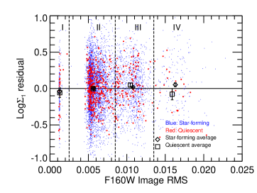
Figure 1.— Comparison of $\Sigma_{1}$ in regions with different depths (indicated by F160W image’s root-mean square error RMS) in CANDELS/GOODS-S. Galaxies are divided into star forming (blue) and quenched (red). For each galaxy, its $\Sigma_{1}$ is compared to the median of galaxies in the Deep region (Region II) with the same redshift, ${\rm M_{*}}$, and star formation activity (star forming or quenched). The difference (individual minus the median) is the $\Sigma_{1}$ deviation in the Y-axis. Squares (and diamonds) with error bars show the 3$\sigma$ clipped mean and standard deviation of the mean for quenched (and star-forming) galaxies. The four regions are: the Hubble Ultra Deep Field (HUDF, I), Deep (II), Wide (III), and Edge (IV) based on the RMS value of the F160W image at the location of the galaxies. The smaller the RMS, the deeper the survey.

We further test the effect of survey depth on the accuracy of $\Sigma_{1}$. We separate galaxies in GOODS-S into regions of the Hubble Ultra Deep Field (HUDF), Deep, Wide, and Edge (which is for edge or corner regions where the depth is very shallow due to the drizzle pattern). The survey depth varies across a range of more than 2.5 mag from the HUDF to the Edge. We choose the Deep region as our fiducial region due to its decent depth and large number of galaxies. For each galaxy in any region, we compare its $\Sigma_{1}$ to the median $\Sigma_{1}$ of galaxies in the Deep region with the same redshift, ${\rm M_{*}}$, and star formation activity (star forming or quenched). The difference (or $\Sigma_{1}$ deviation) is shown in Figure 1. We find no obvious difference between the four regions (the largest deviation is that QGs in the Edge region is about 0.07 dex lower than the other three regions). Moreover, we find no obvious trend of the deviation changes with the survey depth. This test provides strong evidence that if limited to F160W = 25 AB, even though most of CANDELS regions are shallower than HUDF, our $\Sigma_{1}$ measurement has little systematic biases to a population of galaxies regardless of survey depth. The result in Figure 1 shows the statistics of the whole sample. To specifically test the robustness of our $\Sigma_{1}$ measurement in low-mass galaxies, we repeat it for a subsample of low-mass galaxies with ${\rm 10^{8.5}<M_{*}/M_{\odot}<10^{9.5}}$ at $0.5<z<1.0$. The new result, shown in Appendix A, indicates again no significant systematic deviations found between QGs and SFGs across the four survey depths.

We therefore limit our low-mass sample to sources with F160W $H\leq 25$ AB, no suspicious F160W photometry, SExtractor CLASS_STAR$<$0.8, and a clean Sérsic fit flag in van der Wel et al. (2012). To study its corresponding mass limit, we use two stellar population models. The first one represents young galaxies with a constant star formation history and an age of 0.5 Gyr. The second represents old galaxies with a single starburst right after the big bang. This model has the maximum age that a galaxy can have at a given redshift. We then normalize the two models to have the F160W magnitude of 25 AB. The old model (with a high mass-to-light ratio) corresponds to a much higher stellar mass than the young one (Figure 2). We therefore choose the old one as our mass limit at different redshifts. As a sanity check, we also use the empirical formula derived by Chartab et al. (2020) to measure the mass-complete limit of F160W = 25 AB . Their formula is derived by following the method of Pozzetti et al. (2010), which is a common practice in measuring stellar mass functions for large surveys. The empirical limit matches very well with our model limit at $0.5\leq z<2.5$. We therefore determine that our mass limit is $10^{9.2}$${\rm\,M_{\odot}}$ at $0.5\leq z<1.0$, $10^{9.6}$${\rm\,M_{\odot}}$ at $1.0\leq z<1.5$, and $10^{10.0}$${\rm\,M_{\odot}}$ at $1.5\leq z<2.5$ (the three large dotted rectangles in Figure 2). To push our mass limit even lower, we also include galaxies with ${\rm M_{*}}$ between $10^{8.8}$${\rm\,M_{\odot}}$ and $10^{9.2}$${\rm\,M_{\odot}}$ at $0.5\leq z<0.7$, where our sample is also mass complete (the smallest dotted rectangle in Figure 2).

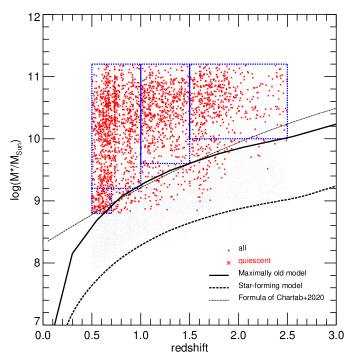
Figure 2.— Sample selection. CANDELS galaxies of $0.5\leq z<2.5$ with F160W H $\leq$ 25 AB are shown as gray points. QGs between $10^{8.8}$ and $10^{11.2}$${\rm\,M_{\odot}}$ are red. The three curves show different estimations of mass completeness of H $\leq$ 25 AB as described in text. The four blue dotted rectangles show our mass-complete sample of QGs at different redshifts.

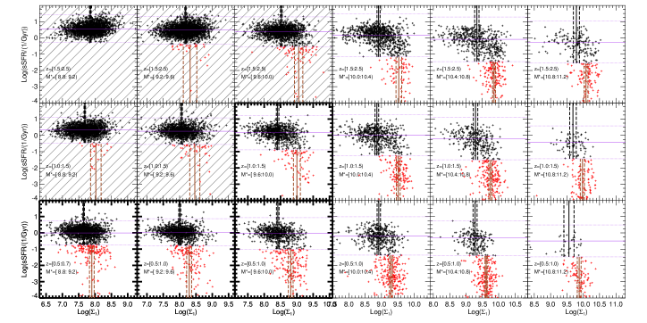
Figure 3.— sSFR as a function of $\Sigma_{1}$ in different redshift and ${\rm M_{*}}$ bins. In each bin, galaxies are divided into SFGs (black) and QGs (red). The horizontal solid and dotted purple lines are the 3$\sigma$ clipped mean sSFR and its 3$\sigma$ deviation for galaxies in the bin. The vertical solid and dashed black (and brown) lines are the 3$\sigma$ clipped mean $\Sigma_{1}$ and the standard deviation of the mean of $\Sigma_{1}$ of SFGs (and QGs). The QG samples in shaded panels are mass incomplete (SFGs are mass complete, though). The four panels toward the bottom left with thick borders highlight the main result of this paper.

3. Results

3.1. Difference of $\Sigma_{1}$ between QGs and SFGs

Figure 3 shows the sSFR as a function of $\Sigma_{1}$ in different redshift and ${\rm M_{*}}$ bins. In each bin, first, for galaxies with sSFR $>10^{-2}/Gyr$, we calculate the 3$\sigma$ clipped mean and standard deviation of the mean of sSFRs (purple solid and dotted lines). Galaxies with an sSFR lower than $-3\sigma$ (the lower dotted line) are classified as QGs, while the others are classified as SFGs. Our mean sSFR and its scatter ($\sigma$) are consistent with those in the literature (e.g., Whitaker et al., 2014; Kurczynski et al., 2016).

Figure 3 shows that, for almost all redshift and ${\rm M_{*}}$ bins, the 3$\sigma$ clipped mean $\Sigma_{1}$ of QGs (solid vertical brown lines) is greater than that of SFGs (solid vertical black lines). Figure 4 shows the statistics.

For massive galaxies (${\rm M_{*}}$$\geq 10^{10}$${\rm\,M_{\odot}}$), at all redshifts, the mean $\Sigma_{1}$ of QGs is significantly ($\gtrsim 10\sigma$) larger than that of SFGs with the same redshift and ${\rm M_{*}}$ (Panel (b) of Figure 4). The difference decreases with ${\rm M_{*}}$. This result is consistent with many other studies at various redshifts (e.g., Cheung et al., 2012; Fang et al., 2013; van Dokkum et al., 2014; Barro et al., 2017; Chen et al., 2020). This difference in $\Sigma_{1}$, combined with no difference in $d_{proj}$ between massive QGs and SFGs found in Guo et al. (2017), demonstrates that internal processes, especially those related to central mass density, e.g., possibly black holes, are the primary way to quench massive galaxies from $z=2.5$ to $z=0.5$ (e.g., Chen et al., 2020) or even to today (e.g., Luo et al., 2020).

The new, interesting result is the $\Sigma_{1}$ comparison in the low-mass regime (i.e., panels highlighted by thick borders in Figure 3). At ${\rm M_{*}}$$\lesssim 10^{9.5}$${\rm\,M_{\odot}}$  we find a $\gtrsim$0.3 dex difference with very high statistical significance ($\gtrsim 5\sigma$) between the mean $\Sigma_{1}$ of QGs and SFGs at $z<1.5$. This result suggests that quenching has a relation with the increase of $\Sigma_{1}$ in low-mass galaxies, similar to the situation of massive galaxies reported by many studies. We will discuss its implications in detail in Section 4.

To remove the mass dependence of $\Sigma_{1}$ further, we calculate the ratio between $\Sigma_{1}$ and ${\rm M_{*}}$ of galaxies (called mass-normalized $\Sigma_{1}$, which is proportional to the fraction of total ${\rm M_{*}}$ within the central 1kpc radius, but differs by a factor of $\pi$). As shown in Panel (c) of Figure 4, this mass-normalized $\Sigma_{1}$ decreases with ${\rm M_{*}}$ for massive QGs. Our trend matches the slope (dashed line) derived through the best-fit $\Sigma_{1}$–${\rm M_{*}}$ relation of QGs from Barro et al. (2017). For low-mass galaxies at $z<1.0$, our QG trend shows a turnover at $10^{10}$${\rm\,M_{\odot}}$, and decreases with the decreasing of ${\rm M_{*}}$. This turnover is mainly a reflection of changes in the Sérsic index ($n$) and size (see Figure 13 of Barro et al. (2017)). For $n\sim 4$ galaxies, the mass-normalized $\Sigma_{1}$ decreases when galaxy size increases. Massive QGs have $n\sim 4$ and their size increases with ${\rm M_{*}}$. Therefore, their mass-normalized $\Sigma_{1}$ decreases with ${\rm M_{*}}$. However, for low-mass QGs at $z\leq 1.0$, their size is flattened in the ${\rm M_{*}}$–size diagram (e.g., van der Wel et al., 2014). Moreover, their $n$ gradually changes from $\sim 4$ to $\sim 1$ with the decrease of ${\rm M_{*}}$. The combination of the two (constant size and decreasing $n$) makes their mass-normalized $\Sigma_{1}$ decreases moderately from the peak at $10^{10}$${\rm\,M_{\odot}}$ and approach a constant value of -1.1 dex. This turnover at $10^{10}$${\rm\,M_{\odot}}$ is also around the stellar mass where quenching mechanisms gradually changes from being dominated by internal processes to by external processes (e.g., Peng et al., 2010; Cybulski et al., 2014; Lee et al., 2015; Darvish et al., 2015, 2016; Wetzel et al., 2015; Balogh et al., 2016; Fillingham et al., 2016; Lin et al., 2016; Guo et al., 2017; Lee et al., 2018).

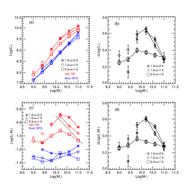
Figure 4.— Statistics of $\Sigma_{1}$. In each panel, different redshifts are shown by different symbols, and different types of galaxies are shown by different colors. Panel (a) shows the 3$\sigma$ clipped mean of $\Sigma_{1}$ as a function of ${\rm M_{*}}$. Panel (b) shows the difference between the 3$\sigma$ clipped mean of $\Sigma_{1}$ of SFGs and QGs ($\Delta$ = QG - SFG). Panel (c) shows the mass-normalized $\Sigma_{1}$ as a function of ${\rm M_{*}}$. The dashed line shows the slope derived from Barro et al. (2017). Panel (d) is similar to Panel (b), but showing the difference between the mass-normalized $\Sigma_{1}$ of SFGs and QGs. In each Panel, symbols connected by lines are mass complete in our sample, while those not connected are mass incomplete.

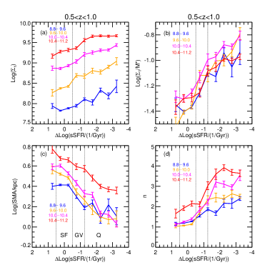
Figure 5.— Relations between different parameters and the residual Log(sSFR) of galaxies at $0.5\leq z<1.0$. The residual Log(sSFR), or $\Delta$Log(sSFR), is defined as the difference between the Log(sSFR) of a galaxy and the average Log(sSFR) of galaxies on the star-forming main sequence at the same redshift and ${\rm M_{*}}$ of the galaxy. Namely, the zero-point of $\Delta$Log(sSFR) corresponds to the solid horizontal purple lines in Figure 3. The four panels show (a) $\Sigma_{1}$, (b) mass-normalized $\Sigma_{1}$ (i.e., Log($\Sigma_{1}$/$M_{*}$), (c) semi-major axis, and (d) Sérsic index. In each panel, galaxies are divided into four ${\rm M_{*}}$ bins, as the labels of different colors show. The curves and error bars show the mean and the standard deviation of the mean (both after 3$\sigma$ clipping) of each ${\rm M_{*}}$ bin. The three vertical black lines show the boundaries of three regions, as indicated in Panel (c): star forming (SF), green valley (GV), and quenched (Q).

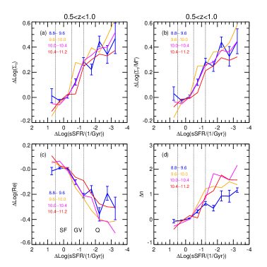
Figure 6.— Similar to Figure 6, but using the residual values (rather than their exact values) for the parameters in the Y-axis. The residual of a parameter is defined as the difference between the parameter of a galaxy and the average of galaxies on the star-forming main sequence at the same redshift and ${\rm M_{*}}$ of the galaxy. For example, $\Delta$Log($\Sigma_{1}$) is defined by using the solid vertical black lines in Figure 3 as the zero-point.

The mass-normalized $\Sigma_{1}$ of SFGs is almost a constant across a wide range of ${\rm M_{*}}$, and is lower than that of their QG counterparts. The difference of mass-normalized $\Sigma_{1}$ between the two populations (Panel (d) of Figure 4) is very similar to that of $\Sigma_{1}$ (Panel (b)). The trend of the mass-normalized $\Sigma_{1}$ of massive SFGs is still uncertain in the literature. For example, Barro et al. (2017) found a sublinear slope (0.88) for the $\Sigma_{1}$–${\rm M_{*}}$ relation, which turns into a mass-normalized $\Sigma_{1}$ slightly decreasing with ${\rm M_{*}}$. Chen et al. (2020) revisited this issue and found a superlinear slope (1.1) for the $\Sigma_{1}$–${\rm M_{*}}$ relation, which implies the mass-normalized $\Sigma_{1}$ slightly increases with ${\rm M_{*}}$. Overall, both slopes are quite close to 1, implying a close-to-flat trend of mass-normalized $\Sigma_{1}$. Therefore, our result of an almost constant trend does not significantly different from either slope.

3.2. $\Sigma_{1}$ and Structural Parameters vs. sSFR

An efficient way to investigate the overall behavior of galaxies over a wide range of parameter space is to use the “residual” plot (e.g., Barro et al., 2017; Woo et al., 2017; Fang et al., 2018; Chen et al., 2020; Lin et al., 2020). Instead of showing the exact values of a parameter, this type of plot shows the relative values of the parameter with respect to a common value, for example, the mean or median of a sample. By taking into account of the different mean or median values of different samples, this method enables a direct comparison between them.

We use the residual plot to show the relations between some parameters and the sSFR. In Figure 5, we only use the residual for the sSFR in the X-axis, but still keep the exact values of other parameters in the Y-axis for readers who are interested in the exact values. In Figure 6, we use the residual for both axes to compare different subsamples with different ${\rm M_{*}}$. The zero-point of the residual is calculated by the average value of galaxies in the star-forming main sequence at a given ($z$, ${\rm M_{*}}$) bin. For example, the zero-point of $\Delta$Log(sSFR) (or $\Delta$Log($\Sigma_{1}$)) is the solid horizontal purple lines (or solid vertical black lines) in Figure 3. Hereinafter, we only focus on the redshift range of $0.5\leq z<1.0$. We also divide galaxies into three categories based on their ${\rm M_{*}}$: low-mass (Log(${\rm M_{*}}$)$<9.6$), intermediate-mass ($9.6\leq$Log(${\rm M_{*}}$)$<10.4$), and massive ($10.4\leq$Log(${\rm M_{*}}$)$<11.2$).

To catch the transition between SFGs and QGs, we divide galaxies into three (rather than previous two) types based on their $\Delta$Log(sSFR): star forming (SF), green valley (GV), and quenched (Q). The divisions are shown in Panel (c) of Figure 5 and 6. They are quite similar to those used in Woo et al. (2017); Liu et al. (2018); Chen et al. (2020). In SF, $\Sigma_{1}$ and $\Sigma_{1}$/${\rm M_{*}}$of galaxies of all ${\rm M_{*}}$ changes little (Panel (a) and (b) of both figures). In GV, all galaxies increases their $\Sigma_{1}$ (or Log($\Sigma_{1}$/${\rm M_{*}}$)) dramatically by about 0.2-0.3 dex. The increase of $\Sigma_{1}$ of massive galaxies during GV has been discussed in Chen et al. (2020, see their Figure 5). Our result shows that intermediate- and low-mass galaxies also follow a similar trend during GV. In Q, galaxies with different ${\rm M_{*}}$ show a slight difference. Massive galaxies reach a plateau of about 0.3 dex in $\Delta$Log($\Sigma_{1}$) or $\Delta$Log($\Sigma_{1}/M_{*}$). This plateau is a reflection of the vertical part of the “elbow” shape in the panels of massive galaxies in Figure 3. This trend and its meaning on quenching have been thoroughly discussed by Barro et al. (2017), Woo et al. (2017), and Chen et al. (2020). On the other hand, intermediate- and low-mass galaxies continue to grow their $\Sigma_{1}$after GV. This trend is especially true for intermediate-mass galaxies, and less obvious for low-mass galaxies due to large uncertainties of small number statistics.

The relation between Log($\Sigma_{1}$) (or $\Delta$Log($\Sigma_{1}$)) and $\Delta$Log(sSFR) is correlated with the change of other structural parameters of galaxies. Panel (c) and (d) of Figure 5 and 6 show the change of size (semimajor axis) and the Sérsic index ($n$). In GV and Q, the sizes of galaxies decrease with $\Delta$Log(sSFR). Low-mass and massive galaxies have a similar decreasing trend, while intermediate-mass galaxies decrease faster. Although intermediate-mass galaxies are larger than low-mass ones in SF, because of this faster decrease, their size approach the size of low-mass galaxies when $\Delta$Log(sSFR) is very low (Panel (c) of Figure 5). This result is consistent with the flattened curve of the size–mass relation of QGs in the low-mass regime (e.g., van der Wel et al., 2014).

Low-mass galaxies and massive galaxies, however, have different trends of $n$. Low-mass galaxies start with a disk-like shape ($n=1$) in SF, then mildly increase $n$ in GV and Q, and finally to reach $n\sim 2$ – still disk-like – in the end of Q. Massive galaxies already start with $n\sim 2$ in SF and quickly increase $n$ during GV and the beginning of Q to $n\sim 4$ (spheroid-like) and remain around $n\sim 4$ in Q. Intermediate-mass galaxies lie between the two extremes. Overall, to summarize, massive galaxies’ plateau of Log($\Sigma_{1}$) at $\Delta$Log(sSFR)$<-2$ correlates with (almost) no change in size and $n$ in Q. Low-mass galaxies’ increasing $\Sigma_{1}$ in Q correlates with a gradual increase of $n$ more than with a slight decrease of size. Intermediate-mass galaxies’ increasing $\Sigma_{1}$ in Q, on the other hand, correlates more with a dramatic decrease of size.

4. Discussion

The main result of this study is the difference between the mean $\Sigma_{1}$ of QGs and SFGs in the low-mass regime (${\rm M_{*}}$$\lesssim 10^{9.5}$${\rm\,M_{\odot}}$) at $z\sim 1$. Similar results have also been reported in the local universe for galaxies with ${\rm M_{*}}$$>10^{9.75}$${\rm\,M_{\odot}}$ in Woo et al. (2017). Here, we discuss some implications of this result for the quenching processes of low-mass galaxies. Although the real quenching processes are very likely to be complicated and complex, our discussions are still useful to place some constraints on quenching and environmental effects.

When we discuss $\Sigma_{1}$ and quenching, it would be very useful to separate low-mass central and satellite galaxies . As shown in Woo et al. (2017), $\Sigma_{1}$ of the transition galaxies (i.e. green-valley galaxies) decreases smoothly with the environment by as much as 0.2 dex for ${\rm M_{*}}$=$10^{9.75}-10^{10}$${\rm\,M_{\odot}}$ galaxies from the field, large halo-centric distance, to small halo-centric distance in SDSS. In our sample, however, due to the limitation of using photometric redshift, galaxy clusters or groups cannot be accurately identified. In Guo et al. (2017), we found that the median projected distance ($d_{proj}$) from low-mass ($M_{*}\lesssim 10^{9.5}$${\rm\,M_{\odot}}$) QGs to their massive ($M_{*}\gtrsim 10^{10.5}$${\rm\,M_{\odot}}$) neighbors is systematically smaller than that of low-mass SFGs. Also, Guo et al. (2017) showed that $\sim 90\%$ of low-mass QGs are within 2 times the virial radius of their neighboring massive halos. These results suggest that (1) on average, low-mass QGs are found closer to massive central galaxies (i.e., higher density region) than low-mass SFGs and (2) most of low-mass QGs tend to be satellite galaxies. Therefore, the results we see in Figure 3 – 6 are likely driven by satellite galaxies.

In next two subsections, we interpret the curves in Figure 5 and 6 as evolutionary tracks. This interpretation is not necessarily true, especially when progenitor bias is considered (Section 4.3). It is, however, still reasonable and useful for our discussion when the change of ${\rm M_{*}}$ of galaxies is small, which is likely true when galaxies quench. The decrease of sSFR results in a moderate increase of ${\rm M_{*}}$, which then keeps most galaxies within their initial ${\rm M_{*}}$ bins, as shown in Figure 5 and 6.

4.1. Low-mass Galaxies in Green Valley

$\Sigma_{1}$ of low-mass galaxies increases by about 0.25 dex in GV, indicating that the quenching mechanisms (possibly environmental effects) gradually quench star formation in an outside-in process, i.e., preferentially removing gas from outskirts of galaxies while maintaining their central star formation to increase $\Sigma_{1}$. We can use the growth of total ${\rm M_{*}}$ and $\Sigma_{1}$ to estimate the timescale of galaxies in GV. We will use the sSFR gradient of low-mass transition galaxies reported in Liu et al. (2018) as our constraint.

We consider a galaxy entering GV with ${\rm M_{*}}$ of $10^{9.2}$${\rm\,M_{\odot}}$ at $z<1.0$. Its sSFR (and hence SFR) can be measured from our sample and is -0.5 dex below the average Log(sSFR) of star-forming main sequence (as defined in Figure 5). When this galaxy exits GV, its sSFR drops by another -0.75 dex to reach -1.25 dex below the star-forming main sequence. Now, we assume this galaxy spends $T_{GV}$=1, 2, and 4 Gyr in GV. Its Log(sSFR) drops linearly with time over this period (i.e., sSFR drops exponentially). Since the change of sSFR is only -0.75 dex, very small compared to the whole sSFR range from SF to Q, the exact form of the decreasing is not important.

For each time step of 0.1 Gyr in GV, based on the galaxy’s current ${\rm M_{*}}$ and sSFR, we calculate its ${\rm M_{*}}$ and sSFR for the next step. From its new ${\rm M_{*}}$, we infer its new $\Sigma_{1}$ from Panel (b) of Figure 5 (or 6). Based on the change in ${\rm M_{*}}$ and $\Sigma_{1}$ in this step, we calculate the SFR (and sSFR) within and outside the central 1 kpc. We repeat this process until the galaxy exits GV. The results are shown in Figure 7.

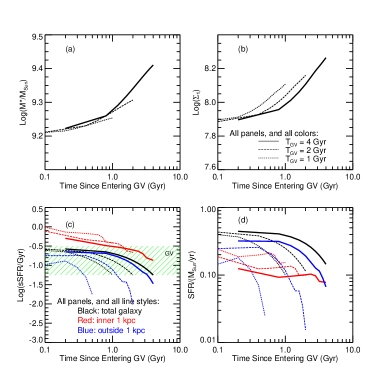
Figure 7.— Growth of a galaxy in GV in our simple models (see Section 4.1). The four panels show (a) ${\rm M_{*}}$, (b) $\Sigma_{1}$, (c) sSFR, and (d) SFR, respectively. In each panel, different line styles show assumptions of different time the galaxy spends in GV, as indicated in Panel (b). In Panel (c) and (d), we also show the curves for the regions within (and outside) the central 1 kpc in red (and blue). The green hatched region in Panel (c) shows the defined GV.

We use two conditions to constrain $T_{GV}$: (1) SFR within central 1 kpc should not exceed the total SFR and (2) the difference between sSFRs within and outside central 1 kpc should match the observed sSFR gradient in Liu et al. (2018), which has a difference of about 0.3 dex within and outside the central 1 kpc (see their Figure 5). The first condition indicates that a small $T_{GV}$ is unlikely. In the case of $T_{GV}$= 1 Gyr (dotted lines in Figure 7), the central SFR exceeds the total SFR in a few hundred million years (compare red and black dotted lines in Panel (d)). The short timescale requires an unrealistically high SFR in the center to boost $\Sigma_{1}$. The case of $T_{GV}$= 2 Gyr meets the first condition, but fails the second one. The difference between the central and outer sSFR is $\gtrsim$0.5 dex (red and blue dashed lines in Panel (c)), which is larger than the observed sSFR difference in Liu et al. (2018). The case of $T_{GV}$=4 Gyr meets both conditions and is therefore most likely to be true. $T_{GV}$ longer than 4 Gyr would produce a much smaller difference between central and outer sSFRs, inconsistent with the observed sSFR gradient in Liu et al. (2018).

Our (rough) estimate of $T_{GV}$ suggests that the time a low-mass galaxy spending on GV is about a few gigayears. If we define this time as the quenching timescale (i.e., time for transitioning from star forming to quenched), our value here is consistent with the quenching timescale estimated by using the dynamics and spatial distribution of quenched low-mass galaxies in large halos in Guo et al. (2017). It is also consistent with the estimate of the quenching timescale of galaxies around $10^{9.5}M_{\odot}$ in Balogh et al. (2016) and Fossati et al. (2017). Ji et al. (2018) also estimated a quenching timescale of a few gigayears ($\sim$4 Gyr) by using the redshift evolution of the clustering strength of CANDELS galaxies. Similarly, Phillipps et al. (2019) found timescales for galaxies crossing GV at lower redshifts $0.1<z<0.2$ is also a few gigayears (2-4 Gyr). Overall, the quenching of low-mass galaxies is not rapid, but rather a gradual and long processes. The quenching timescale can be used to test quenching mechanisms, which need to, not only reduce the total and outskirt SFR by a factor of 3 in a few gigayears, but also maintain the central (within 1 kpc) SFR almost constant over this long period (see solid lines in Panel (d) of Figure 7).

The long quenching timescale of low-mass galaxies is consistent with the low quenching efficiency measured in many studies. For example, Kawinwanichakij et al. (2017), Papovich et al. (2018), and Chartab et al. (2020) all found that the environmental quenching efficiency decreases with the decrease of ${\rm M_{*}}$. The mass quenching efficiency also decreases with the decrease of ${\rm M_{*}}$ (e.g., Chartab et al., 2020). Both efficiencies are quite low at ${\rm M_{*}}$$<10^{9.5}$${\rm\,M_{\odot}}$ (Kawinwanichakij et al., 2017; Chartab et al., 2020; Contini et al., 2020). Therefore, the quenching timescale is expected to be long.

One model to explain the quenching of low-mass galaxies involves both “starvation” (i.e., cutting off gas supplies by environmental effects (e.g., Larson et al., 1980; Balogh et al., 1997)) and “overconsumption” (i.e., gas depletion because of star formation and star-formation driven outflows (McGee et al., 2014)). The gas depletion time is shorter at high redshifts when SFR is higher, but increases with the cosmic time. In fact, the gas depletion time for GV galaxies at $z<1.0$ is about a few gigayears (inferred from Genzel et al., 2015), consistent with our estimate of the quenching timescale. In a recent paper, Trussler et al. (2020) found that quenching is driven by both starvation and outflow, and they estimated the quenching timescale is a few to several gigayears (depending on the models) in the local universe. Moutard et al. (2018), however, argued for a delayed-then-rapid quenching scenario (Wetzel et al., 2013), where quenching of low-mass galaxies is rapid (a few hundred megayears) after a long period since entering high-density regions.

The long quenching timescale also allows GV galaxies to transform their morphology while quenching their star formation in gradual processes. Kawinwanichakij et al. (2017) found that the morphologies of lower-mass QGs are inconsistent with those expected of recently quenched SFGs. Our results are consistent with their conclusion, as both $\Sigma_{1}$ and the Sérsic index ($n$, although only mildly) increase when low-mass galaxies evolve from SF to GV, and eventually to Q, as shown in Figure 5. Kawinwanichakij et al. (2017) argued that simple gas removal processes, e.g., strangulation and ram pressure, are not able to transform morphology and therefore some dynamical processes need to be involved, e.g., galaxy interactions, tidal stripping, and disk fading. Our results, however, suggest that the long star formation duration ($\sim 4$ Gyr) in central region is able to increase $\Sigma_{1}$ and $n$.

4.2. Low-mass Galaxies after Green Valley

Once a low-mass galaxy exits GV, its total sSFR drops to at least -1.25 dex lower than the star-forming main sequence, and is therefore too low to form many new stars to effectively increase its total ${\rm M_{*}}$. Its $\Sigma_{1}$, however, still increases. For example, when the galaxy we discuss in Figure 7 exits GV after 4 Gyr, its ${\rm M_{*}}$=$10^{9.4}$${\rm\,M_{\odot}}$, and its Log($\Sigma_{1}$) is 8.25 (solid black lines in Panel (a) and (b)). From the blue curve of Panel (b) of Figure 5, we know that galaxies with similar ${\rm M_{*}}$ would have Log($\Sigma_{1}$/${\rm M_{*}}$) of -0.95 in the end of Q (the blue curve at $\Delta$Log(sSFR)$<-2$), corresponding to a $\Sigma_{1}$ of 8.45. Therefore, its $\Sigma_{1}$ increases by 0.2 dex in Q. Since few new stars are formed in this period, the galaxy cannot increase its $\Sigma_{1}$ by star formation.

Therefore, $\Sigma_{1}$ has to be increased by some environmental effects through the redistribution of existing stars. Most effects, e.g., harassment and tidal stripping, tend to make satellite galaxies more extended rather than more concentrated while reducing their overall ${\rm M_{*}}$ (e.g., Carleton et al., 2019; Tremmel et al., 2019). A scenario, however, is possible to effectively “increase” $\Sigma_{1}$: if harassment or tidal stripping only remove outskirt stars of a galaxy while keeping its center intact, the galaxy will keep the same $\Sigma_{1}$ but move to lower ${\rm M_{*}}$, equivalent to increasing its $\Sigma_{1}$/${\rm M_{*}}$ (see Woo et al., 2017, and references therein). In our example above, to match the observed Log($\Sigma_{1}$/${\rm M_{*}}$)$\sim$-0.95 at $\Delta$Log(sSFR)$<$-3 in Q, the galaxy needs to lose about 30%-40% ($\sim$0.2 dex) of its ${\rm M_{*}}$ after exiting GV.

The mass loss of satellite halos due to environmental effects is well studied. For example, Jiang & van den Bosch (2016) showed that a $10^{11}$${\rm\,M_{\odot}}$ halo orbiting a $10^{13}$${\rm\,M_{\odot}}$ halo loses half its mass in about 2.5 Gyr. Lee et al. (2018) also show that if subject to tidal stripping of a massive neighboring halo, halos around $10^{11}$${\rm\,M_{\odot}}$ often lose a large fraction ($>20\%$) of their peak mass. The fraction of the lost halo mass seems to match the required ${\rm M_{*}}$ loss discussed above, but satellite galaxies lose halo mass more easily than losing ${\rm M_{*}}$. As shown in Engler et al. (2021), the ${\rm M_{*}}$–${\rm M_{halo}}$ relation of satellite galaxies is higher than that of central galaxies. Therefore, once becoming a satellite, a galaxy would lose a much higher fraction of its initial halo mass than the fraction of its initial ${\rm M_{*}}$. As inferred from Errani et al. (2018), the loss of $\sim$50% of halo mass is only corresponding to the loss of a few percents of ${\rm M_{*}}$, much lower than the needed 30%–40% discussed above. In order to lose 30%–40% of ${\rm M_{*}}$, satellite halos need to lose $\gtrsim 90\%$ of their halo mass, which seems too high to be true.

4.3. Progenitor Bias

One alternative explanation of the “increase” of $\Sigma_{1}$ in Q is progenitor bias. It is used to explain some observed redshift evolution of galaxy properties, e.g., the size of massive QGs (e.g., Belli et al., 2015; Keating et al., 2015; Shankar et al., 2015) and the increase of massive QGs’ $\Sigma_{1}$ with redshift (Tacchella et al., 2017). In the redshift evolution of QGs’ size–mass relation, newly quenched systems have larger sizes and therefore increase the average size of the quenched pool toward low redshifts.

Similarly, progenitor bias suggests that low-mass galaxies with the highest $\Sigma_{1}$ at low redshifts are quenched at higher redshifts, when galaxies have higher surface mass densities. These earlier quenched systems increases the average $\Sigma_{1}$ of the quenched pool at low redshifts when comparing it to low-redshift SFGs. This explanation is possible, as high-redshift QGs have higher $\Sigma_{1}$ than low-redshift QGs at the same ${\rm M_{*}}$ (Figure 4). It, however, has another requirement: high-redshift low-mass QGs need to have higher $\Sigma_{1}$ than their SFG counterparts. Low-mass SFGs (down to $10^{9}$${\rm\,M_{\odot}}$) in our highest-redshift bin $1.5\leq z<2.5$ (where our sample is still mass-complete, as shown in Figure 2) have a lower $\Sigma_{1}$ than QGs in our lowest-redshift bin ($0.5\leq z<1.0$). Therefore, if low-mass QGs at $z\sim 2$ have a similar average $\Sigma_{1}$ as low-mass SFGs at $z\sim 2$, they are not able to explain the higher end of $\Sigma_{1}$ of the low-redshift low-mass QGs. High-redshift low-mass QGs need to have a $\sim$0.4-0.5 dex higher $\Sigma_{1}$ than their SFGs counterparts to validate the explanation.

There are two ways to satisfy this requirement. First, only SFGs with the highest $\Sigma_{1}$ are able to quench. At ${\rm M_{*}}$$\sim$$10^{9}$${\rm\,M_{\odot}}$, the highest Log($\Sigma_{1}$) of SFGs at $z\sim 2$ is $>$8.5 (see the shaded panels in Figure 3). This value is high enough to explain the high-end of $\Sigma_{1}$ around ${\rm M_{*}}$$\sim$$10^{9}$${\rm\,M_{\odot}}$ at $z<1.0$. This way implies that high $\Sigma_{1}$ at high redshifts is a direct indicator of quenching and therefore that internal quenching could be important for low-mass galaxies at high redshifts. The second way is that high-redshift low-mass galaxies also undergo the dramatic growth of $\Sigma_{1}$ in GV, similar to what we discussed in Section 4.1. The second way is preferred, because we do see a range of $\Sigma_{1}$ in high-redshift low-mass QGs from Figure 3 (even with a mass-incomplete sample), which is inconsistent with the assumption of the first way that only the low-mass SFGs with the highest $\Sigma_{1}$ at $z\sim 2$ are able to quench.

A few further observations can test the progenitor bias in low-mass galaxies. (1) A mass-complete sample at high redshift and low mass is needed to test the difference in $\Sigma_{1}$ between SFGs and QGs. (2) The number density of QGs at high redshifts (and with high $\Sigma_{1}$) should match that of QGs with the highest $\Sigma_{1}$ in low redshift. (3) $\Sigma_{1}$should correlates with the age of stellar population of QGs. Namely, the higher the $\Sigma_{1}$, the older the QGs.

4.4. Similarity and Difference between Low-mass and Massive Galaxies

An interesting and intriguing result of our study is the similarity between low-mass ($\lesssim 10^{9.5}M_{\odot}$) and massive ($\gtrsim 10^{10.4}M_{\odot}$) galaxies at $0.5\leq z<1.0$ in the relation between $\Delta$Log($\Sigma_{1}$) (or $\Delta$Log($\Sigma_{1}$/${\rm M_{*}}$)) and $\Delta$Log(sSFR) (see Panel (a) and (b) of Figure 6). This similarity is especially true for the dramatic increase of $\Sigma_{1}$ in GV.

As discussed in Section 1, $\Sigma_{1}$ has been shown to be an effective indicator of internal quenching of massive galaxies, possibly correlated with supermassive black hole mass. Chen et al. (2020) found that for massive galaxies, most black hole mass growth takes place in GV. If low-mass galaxies are a scale-down of massive galaxies, the physical processes that build up black hole mass and $\Sigma_{1}$ and that provide feedback from high $\Sigma_{1}$ in massive galaxies could also work in low-mass galaxies.

In fact, recent studies found evidence of a central engine to provide feedback in low-mass galaxies. Bradford et al. (2018) found deficiencies of HI gas in isolated AGN-host low-mass galaxies, suggesting that black hole feedback or shocks from extreme starburst destroy or consume the cold gas. Stellar feedback (related with central starburst) has been considered to be a major effect for low-mass galaxies, since the fraction of AGN hosts decreases with ${\rm M_{*}}$, and so does the importance of black hole/AGN feedback (see Kaviraj et al., 2019, though). However, a large sample of low-mass galaxies have been found to have signatures of black holes (Reines et al., 2013; Reines & Volonteri, 2015), providing the sources of the central engines of quenching. greene20 suggested that a high fraction of $10^{9}-10^{10}M_{\odot}$ galaxies hosting intermediate-mass black holes. Penny et al. (2018) found evidence for AGN feedback in a subset of 69 quenched low-mass galaxies (in groups) in the MANGA survey. Their result demonstrates the importance of AGN feedback in maintaining quiescence of low-mass galaxies.

A few differences, however, exist between low-mass and massive galaxies. First, as we discussed in Introduction, the physical meaning of $\Sigma_{1}$ may be different for the two populations. In massive galaxies, $\Sigma_{1}$ samples well the core mass surface density, while in low-mass galaxies, it represents more the inner density within a large portion of the effective radius. Second, low-mass QGs do not have a classical bulge, while massive galaxies do. This difference is evident by the Sérsic index of both populations ($n\sim 2$ for low-mass QGs and $n\sim 4$ for massive QGs, as shown in Panel (d) of Figure 5). Last, low-mass SFGs and QGs are found to have different projected distances to massive galaxies (Guo et al., 2017), indicating different impacts of environmental effects.

The role of the increased $\Sigma_{1}$ in low-mass galaxies could be a “preprocessing” of quenching. Socolovsky et al. (2019) found that in dense environments at $z<1$, compact low-mass SFGs (which would have a higher $\Sigma_{1}$ at a given ${\rm M_{*}}$) are preferentially quenched. They proposed that both strong feedback and environmental effects act together to quickly quench them. By stacking spectra of high-sSFR galaxies, they even found that more compact galaxies are more likely to host outflows. Their results are broadly consistent with ours, both indicating that low-mass galaxies with high $\Sigma_{1}$ are more easily to be quenched than those with a low $\Sigma_{1}$ when they fall into a dense environment. Guo et al. (2016) showed that the star formation history of low-mass galaxies is bursty at $z\gtrsim 1$. Star formation can temporarily quench these galaxies, but new gas accretion and recycling induce new episodes of starburst. To fully quench them, some effects, potentially environmental, are required to turn off the continuous gas supply.

5. Summary

We use CANDELS data to study the relationship between the central stellar mass surface density ($\Sigma_{1}$) and quenching of low-mass galaxies at $0.5\leq z<1.5$, Our mass-complete sample allows us to investigate galaxies down to $\sim 10^{9}$${\rm\,M_{\odot}}$ at $0.5\leq z<1.0$ with reliable $\Sigma_{1}$ measurements. At a given redshift and ${\rm M_{*}}$ bin, we compare the mean $\Sigma_{1}$ of QGs and SFGs. We find that for massive (${\rm M_{*}}$ $>10^{10}$${\rm\,M_{\odot}}$) galaxies, QGs have significantly higher average $\Sigma_{1}$ than SFGs, consistent with other studies in the literature. Intriguingly, we find that low-mass QGs also have a higher $\Sigma_{1}$ than low-mass SFGs at $z\sim 1$. At $z\leq 1.0$, the difference of $\Sigma_{1}$ between QGs and SFGs increases slightly with ${\rm M_{*}}$ at $\lesssim 10^{10}$${\rm\,M_{\odot}}$ and then decreases with ${\rm M_{*}}$ for more massive galaxies.

We use $\Delta$Log(sSFR), namely, the difference between galaxies’ Log(sSFR) and that of the star-forming main sequence at the same $z$ and ${\rm M_{*}}$, to further divide galaxies into three categories: SF, GV, and Q. At $0.5\leq z<1.0$, we find that the $\Sigma_{1}$ of galaxies increases dramatically in GV, by about 0.25 dex, regardless of their ${\rm M_{*}}$. In Q, massive galaxies reach a plateau in $\Sigma_{1}$, which correlates with (almost) no change of size and $n$. Low-mass galaxies’ increasing $\Sigma_{1}$ in Q correlates more with a gradual increase of $n$, while intermediate-mass galaxies’ increasing $\Sigma_{1}$ in Q correlates more with a dramatic decrease of size.

We use the growth of ${\rm M_{*}}$ and $\Sigma_{1}$ of low-mass galaxies in GV to constrain their time spent in GV. By matching the observed sSFR gradient in Liu et al. (2018), we estimate that the quenching timescale of low-mass galaxies is a few ($\sim 4$) Gyr at $z<1.0$. Quenching mechanisms need to gradually quench star formation in an outside-in way, i.e., preferentially removing gas from outskirts of galaxies while maintaining their central star formation to increase $\Sigma_{1}$. In Q, the increase of $\Sigma_{1}$ in low-mass QGs is still unknown, with possible explanations including dynamical processes and/or progenitor bias.

We also discuss the similarity and difference between low-mass and massive galaxies. Although environmental effects are believed to dominate the quenching of low-mass galaxies, the similar trend of $\Delta$Log($\Sigma_{1}$) vs. $\Delta$Log(sSFR) suggests that internal processes in quenching low-mass galaxies should also be investigated. Future studies can improve our understanding in a few aspects: (1) using a mass-complete sample to explore low-mass galaxies at higher redshifts and (2) investigating black holes/AGN in low-mass galaxies and their relation to galaxy properties (e.g., central mass density) in all environments.

The authors thank the anonymous referee for providing valuable comments, which improved the manuscript. Support for Program number HST-AR-13891, HST-AR-15025, and HST-GO-12060 were provided by NASA through a grant from the Space Telescope Science Institute, which is operated by the Association of Universities for Research in Astronomy, Incorporated, under NASA contract NAS5-26555. Members of the CANDELS team at UCSC acknowledge support from NASA HST grant GO-12060.10-A and from NSF grants AST-0808133 and AST-1615730. SL acknowledges the support from the National Research Foundation of Korea (NRF) grant (2020R1I1A1A01060310) funded by the Korean government (MSIP).

Appendix A Robustness of $\Sigma_{1}$ Measurement in Low-mass Galaxies

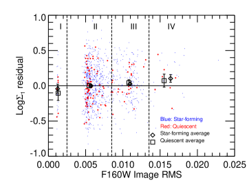
Figure 8.— Same as Figure 1 but only using galaxies with $8.5<{\rm log(M_{*}/M_{\odot})}<9.5$ at $0.5<z<1.0$.

To further investigate the robustness of our $\Sigma_{1}$ measurement in low-mass galaxies, we repeat our test of $\Sigma_{1}$ deviation as a function of the depth of GOODS-S image (Figure 1) using only low-mass galaxies ($8.5<{\rm log(M_{*}/M_{\odot})}<9.5$) at $0.5<z<1.0$. The result, shown in Figure 8, demonstrates that our $\Sigma_{1}$ measurement is unbiased for low-mass (and therefore relatively faint) galaxies in the Deep and Shallow regions. Small deviations exists in the regions of HUDF (Region I) and Edge (Region IV), where the numbers of galaxies are quite low. What is important in the result is that the two populations (QGs and SFGs) have very similar deviations (if there is any) from zero. This similarity indicates that the small deviations do not introduce a significant systematical difference between the two populations. Therefore, our $\Sigma_{1}$ measurement is not only unbiased for the statistics of the whole sample (as in Figure 1), but also introducing no bias to the two populations in the low-mass sample.

Appendix B Effect of PSF Correction

It is important to test if our observed trend of the difference of $\Sigma_{1}$ between QGs and SFGs is driven by the PSF correction. To this purpose, in Figure 9, we plot the PSF correction factor, namely, the corrected ${\rm Log\Sigma_{1}}$ minus the raw, uncorrected ${\rm Log\Sigma_{1}}$, as a function of the size (semimajor axis) of galaxies. For low-mass galaxies (${\rm Log(M_{*}/M_{\odot})<10}$) at $z<1$, the average correction is about 0.2 dex, with QGs (red in the figure) having a slightly larger correction factor than SFGs (black in the figure). The difference between the correction factors of the two populations is around 0.05 dex. This difference is much smaller than the observed difference between the two populations (e.g., in Figure 3 and Panel (b) of Figure 4). Therefore, our main result of low-mass QGs having a higher $\Sigma_{1}$ than low-mass SFGs is not driven by the PSF correction.

To demonstrate this point directly, we compare the raw $\Sigma_{1}$ of the two populations in Figure 10. This figure shows that even without PSF correction, the raw data already display a statistically significant difference between the two populations (i.e., QGs have a higher $\Sigma_{1}$ than SFGs at low mass). The statistics of the difference is plotted in Figure 11. Comparing it to Figure 4, we find that the PSF correction only slightly enhances the difference between QGs and SFGs. This enhancement is reasonable and necessary, because low-mass QGs, which have a slightly higher Sérsic index than low-mass SFGs, are more affected by the PSF and therefore need larger correction factors. Moreover, Figure 11 shows that the trend of $\Delta\Sigma_{1}$ vs. ${\rm Log(M_{*})}$ is quite similar to that in Figure 4.

In principle, the PSF correction should also depend on the size of galaxies. We argue that, however, size is only the secondary parameter in the PSF correction. In fact, in Figure 9, the correction factor already shows a dependence on galaxies’ sizes, even though we do not include size dependence in our correction method. This result is due to the coupling of the size and the Sérsic index $n$ in the Sérsic profiles. Our argument is consistent with the result of Trujillo et al. (2001a), who found that $n$ is the parameter most affected by seeing. In another paper, Trujillo et al. (2001b) showed that when the effective radius of galaxies is comparable or larger than the FWHM of the PSF, the effect of the PSF on the mean effective surface brightness (a good proximity to our $\Sigma_{1}$for low-mass galaxies) is almost independent of galaxies’ radii. Therefore, we believe that not including size dependence in our PSF correction does not significantly affect our results. Moreover, since smaller galaxies (e.g., low-mass QGs) are more affected by the PSF than larger galaxies (e.g., low-mass SFGs), if we included the size effect in PSF correction, the correction factor of low-mass QGs (or SFGs) would have been larger (or smaller) than what we used in the paper. As a result, the difference between the $\Sigma_{1}$ of the two populations would be even larger, strengthening our conclusion of low-mass QGs having a higher $\Sigma_{1}$. For example, for galaxies with ${\rm 9.6<Log(M_{*}/M_{\odot})<10}$ at $z<1$, if we considered the size dependence in the PSF correction, the difference of $\Sigma_{1}$ between QGs and SFGs would be larger than our reported value by $\sim$0.11 dex. For lower-mass (or more massive) galaxies at $z<1$, the extra difference of $\Sigma_{1}$ between QGs and SFGs introduced by considering size dependence is smaller (or larger).

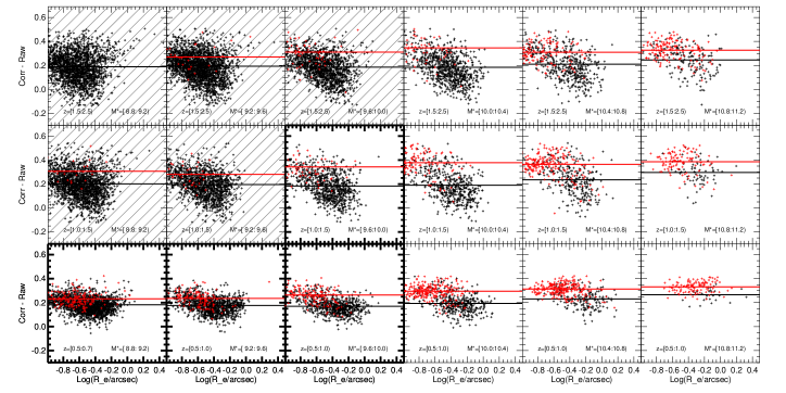
Figure 9.— PSF correction factor as a function of the size (semimajor axis) of the galaxies in our sample. The correction factor (Y-axis) is the difference between the PSF-corrected ${\rm Log\Sigma_{1}}$ and the uncorrected (raw) ${\rm Log\Sigma_{1}}$. The symbols and color schemes are the same as in Figure 3. The red and black horizontal lines show the average of the QGs and SFGs, respectively.

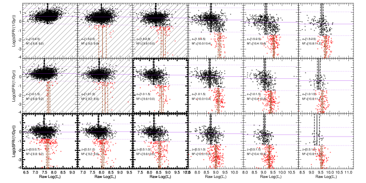
Figure 10.— Same as Figure 3 but using the raw $\Sigma_{1}$ (uncorrected for PSF effects). The difference of $\Sigma_{1}$ between QGs and SFGs is already statistically significant in this case.

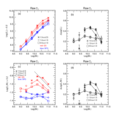
Figure 11.— Same as Figure 4 but using the raw $\Sigma_{1}$ (uncorrected for PSF effects). Data in Panel (a) and (c) are arbitrarily moved up by 0.2 dex to keep the same Y-axis range as in Figure 4 for a direct comparison of the slopes.

References

- Balogh et al. (1997) Balogh, M. L., Morris, S. L., Yee, H. K. C., Carlberg, R. G., & Ellingson, E. 1997, ApJ, 488, L75
- Balogh et al. (2016) Balogh, M. L., McGee, S. L., Mok, A., et al. 2016, MNRAS, 456, 4364
- Barro et al. (2017) Barro, G., Faber, S. M., Koo, D. C., et al. 2017, ApJ, 840, 47
- Belli et al. (2015) Belli, S., Newman, A. B., & Ellis, R. S. 2015, ApJ, 799, 206
- Bradford et al. (2018) Bradford, J. D., Geha, M. C., Greene, J. E., Reines, A. E., & Dickey, C. M. 2018, ApJ, 861, 50
- Calzetti et al. (2000) Calzetti, D., Armus, L., Bohlin, R. C., et al. 2000, ApJ, 533, 682
- Carleton et al. (2019) Carleton, T., Errani, R., Cooper, M., et al. 2019, MNRAS, 485, 382
- Chabrier (2003) Chabrier, G. 2003, PASP, 115, 763
- Chartab et al. (2020) Chartab, N., Mobasher, B., Darvish, B., et al. 2020, ApJ, 890, 7
- Chen et al. (2020) Chen, Z., Faber, S. M., Koo, D. C., et al. 2020, ApJ, 897, 102
- Cheung et al. (2012) Cheung, E., Faber, S. M., Koo, D. C., et al. 2012, ApJ, 760, 131
- Contini et al. (2020) Contini, E., Gu, Q., Ge, X., et al. 2020, ApJ, 889, 156
- Cybulski et al. (2014) Cybulski, R., Yun, M. S., Fazio, G. G., & Gutermuth, R. A. 2014, MNRAS, 439, 3564
- Dahlen et al. (2013) Dahlen, T., Mobasher, B., Faber, S. M., et al. 2013, ApJ, 775, 93
- Darvish et al. (2016) Darvish, B., Mobasher, B., Sobral, D., et al. 2016, ApJ, 825, 113
- Darvish et al. (2015) Darvish, B., Mobasher, B., Sobral, D., Scoville, N., & Aragon-Calvo, M. 2015, ApJ, 805, 121
- De Lucia et al. (2019) De Lucia, G., Hirschmann, M., & Fontanot, F. 2019, MNRAS, 482, 5041
- Engler et al. (2021) Engler, C., Pillepich, A., Joshi, G. D., et al. 2021, MNRAS, 500, 3957
- Errani et al. (2018) Errani, R., Peñarrubia, J., & Walker, M. G. 2018, MNRAS, 481, 5073
- Fang et al. (2013) Fang, J. J., Faber, S. M., Koo, D. C., & Dekel, A. 2013, ApJ, 776, 63
- Fang et al. (2018) Fang, J. J., Faber, S. M., Koo, D. C., et al. 2018, ApJ, 858, 100
- Fillingham et al. (2016) Fillingham, S. P., Cooper, M. C., Pace, A. B., et al. 2016, MNRAS, 463, 1916
- Fillingham et al. (2015) Fillingham, S. P., Cooper, M. C., Wheeler, C., et al. 2015, MNRAS, 454, 2039
- Fossati et al. (2017) Fossati, M., Wilman, D. J., Mendel, J. T., et al. 2017, ApJ, 835, 153
- Galametz et al. (2013) Galametz, A., Grazian, A., Fontana, A., et al. 2013, ApJS, 206, 10
- Geha et al. (2012) Geha, M., Blanton, M. R., Yan, R., & Tinker, J. L. 2012, ApJ, 757, 85
- Genzel et al. (2015) Genzel, R., Tacconi, L. J., Lutz, D., et al. 2015, ApJ, 800, 20
- Grogin et al. (2011) Grogin, N. A., Kocevski, D. D., Faber, S. M., et al. 2011, ApJS, 197, 35
- Guo et al. (2009) Guo, Y., McIntosh, D. H., Mo, H. J., et al. 2009, MNRAS, 398, 1129
- Guo et al. (2013) Guo, Y., Ferguson, H. C., Giavalisco, M., et al. 2013, ApJS, 207, 24
- Guo et al. (2016) Guo, Y., Rafelski, M., Faber, S. M., et al. 2016, ApJ, 833, 37
- Guo et al. (2017) Guo, Y., Bell, E. F., Lu, Y., et al. 2017, ApJ, 841, L22
- Ji et al. (2018) Ji, Z., Giavalisco, M., Williams, C. C., et al. 2018, ApJ, 862, 135
- Jiang & van den Bosch (2016) Jiang, F., & van den Bosch, F. C. 2016, MNRAS, 458, 2848
- Kaviraj et al. (2019) Kaviraj, S., Martin, G., & Silk, J. 2019, MNRAS, 489, L12
- Kawinwanichakij et al. (2017) Kawinwanichakij, L., Papovich, C., Quadri, R. F., et al. 2017, ApJ, 847, 134
- Keating et al. (2015) Keating, S. K., Abraham, R. G., Schiavon, R., et al. 2015, ApJ, 798, 26
- Koekemoer et al. (2011) Koekemoer, A. M., Faber, S. M., Ferguson, H. C., et al. 2011, ApJS, 197, 36
- Kriek et al. (2009) Kriek, M., van Dokkum, P. G., Labbé, I., et al. 2009, ApJ, 700, 221
- Kurczynski et al. (2016) Kurczynski, P., Gawiser, E., Acquaviva, V., et al. 2016, ApJ, 820, L1
- Larson et al. (1980) Larson, R. B., Tinsley, B. M., & Caldwell, C. N. 1980, ApJ, 237, 692
- Lee et al. (2018) Lee, C. T., Primack, J. R., Behroozi, P., et al. 2018, MNRAS, 481, 4038
- Lee et al. (2015) Lee, S.-K., Im, M., Kim, J.-W., et al. 2015, ApJ, 810, 90
- Lilly & Carollo (2016) Lilly, S. J., & Carollo, C. M. 2016, ApJ, 833, 1
- Lin et al. (2016) Lin, L., Capak, P. L., Laigle, C., et al. 2016, ApJ, 817, 97
- Lin et al. (2020) Lin, L., Faber, S. M., Koo, D. C., et al. 2020, ApJ, 899, 93
- Liu et al. (2016) Liu, F. S., Jiang, D., Guo, Y., et al. 2016, ApJ, 822, L25
- Liu et al. (2018) Liu, F. S., Jia, M., Yesuf, H. M., et al. 2018, ApJ, 860, 60
- Luo et al. (2020) Luo, Y., Faber, S. M., Rodríguez-Puebla, A., et al. 2020, MNRAS, 493, 1686
- McGee et al. (2014) McGee, S. L., Bower, R. G., & Balogh, M. L. 2014, MNRAS, 442, L105
- Miller et al. (2019) Miller, T. B., van Dokkum, P., Mowla, L., & van der Wel, A. 2019, ApJ, 872, L14
- Moutard et al. (2018) Moutard, T., Sawicki, M., Arnouts, S., et al. 2018, MNRAS, 479, 2147
- Mowla et al. (2019) Mowla, L., van der Wel, A., van Dokkum, P., & Miller, T. B. 2019, ApJ, 872, L13
- Nayyeri et al. (2017) Nayyeri, H., Hemmati, S., Mobasher, B., et al. 2017, ApJS, 228, 7
- Oke (1974) Oke, J. B. 1974, ApJS, 27, 21
- Papovich et al. (2018) Papovich, C., Kawinwanichakij, L., Quadri, R. F., et al. 2018, ApJ, 854, 30
- Peng et al. (2010) Peng, Y., Lilly, S. J., Kovač, K., et al. 2010, ApJ, 721, 193
- Peng et al. (2012) Peng, Y.-j., Lilly, S. J., Renzini, A., & Carollo, M. 2012, ApJ, 757, 4
- Penny et al. (2018) Penny, S. J., Masters, K. L., Smethurst, R., et al. 2018, MNRAS, 476, 979
- Phillipps et al. (2019) Phillipps, S., Bremer, M. N., Hopkins, A. M., et al. 2019, MNRAS, 485, 5559
- Pozzetti et al. (2010) Pozzetti, L., Bolzonella, M., Zucca, E., et al. 2010, A&A, 523, A13
- Reines et al. (2013) Reines, A. E., Greene, J. E., & Geha, M. 2013, ApJ, 775, 116
- Reines & Volonteri (2015) Reines, A. E., & Volonteri, M. 2015, ApJ, 813, 82
- Santini et al. (2015) Santini, P., Ferguson, H. C., Fontana, A., et al. 2015, ApJ, 801, 97
- Shankar et al. (2015) Shankar, F., Buchan, S., Rettura, A., et al. 2015, ApJ, 802, 73
- Socolovsky et al. (2019) Socolovsky, M., Maltby, D. T., Hatch, N. A., et al. 2019, MNRAS, 482, 1640
- Stefanon et al. (2017) Stefanon, M., Yan, H., Mobasher, B., et al. 2017, ApJS, 229, 32
- Tacchella et al. (2017) Tacchella, S., Carollo, C. M., Faber, S. M., et al. 2017, ApJ, 844, L1
- Tacchella et al. (2015) Tacchella, S., Carollo, C. M., Renzini, A., et al. 2015, Science, 348, 314
- Terrazas et al. (2016) Terrazas, B. A., Bell, E. F., Henriques, B. M. B., et al. 2016, ApJ, 830, L12
- Tremmel et al. (2019) Tremmel, M., Wright, A. C., Brooks, A. M., et al. 2019, arXiv e-prints, arXiv:1908.05684
- Trujillo et al. (2001a) Trujillo, I., Aguerri, J. A. L., Cepa, J., & Gutiérrez, C. M. 2001a, MNRAS, 321, 269
- Trujillo et al. (2001b) Trujillo, I., Aguerri, J. A. L., Cepa, J., & Gutiérrez, C. M. 2001b, MNRAS, 328, 977
- Trussler et al. (2020) Trussler, J., Maiolino, R., Maraston, C., et al. 2020, MNRAS, 491, 5406
- van der Wel et al. (2012) van der Wel, A., Bell, E. F., Häussler, B., et al. 2012, ApJS, 203, 24
- van der Wel et al. (2014) van der Wel, A., Franx, M., van Dokkum, P. G., et al. 2014, ApJ, 788, 28
- van Dokkum et al. (2014) van Dokkum, P. G., Bezanson, R., van der Wel, A., et al. 2014, ApJ, 791, 45
- Wang et al. (2018a) Wang, E., Wang, H., Mo, H., et al. 2018a, ApJ, 864, 51
- Wang et al. (2020) Wang, E., Wang, H., Mo, H., van den Bosch, F. C., & Yang, X. 2020, ApJ, 889, 37
- Wang et al. (2018b) Wang, E., Wang, H., Mo, H., et al. 2018b, ApJ, 860, 102
- Wetzel et al. (2013) Wetzel, A. R., Tinker, J. L., Conroy, C., & van den Bosch, F. C. 2013, MNRAS, 432, 336
- Wetzel et al. (2015) Wetzel, A. R., Tollerud, E. J., & Weisz, D. R. 2015, ApJ, 808, L27
- Wheeler et al. (2014) Wheeler, C., Phillips, J. I., Cooper, M. C., Boylan-Kolchin, M., & Bullock, J. S. 2014, MNRAS, 442, 1396
- Whitaker et al. (2014) Whitaker, K. E., Franx, M., Leja, J., et al. 2014, ApJ, 795, 104
- Woo et al. (2017) Woo, J., Carollo, C. M., Faber, S. M., Dekel, A., & Tacchella, S. 2017, MNRAS, 464, 1077