Abstract

It is challenging to construct explicit and controllable models that realize de Sitter solutions in string compactifications. This difficulty is the main motivation for the Refined de Sitter Conjecture and the Trans-Planckian Censorship Conjecture which forbid stable de Sitter solutions but allow metastable, unstable and rolling solutions in a theory consistent with quantum gravity. Inspired by this, we first study a toy de Sitter No-Scale Supergravity model and show that for particular choices of parameters it can be consistent with the Refined de Sitter Conjecture and the Trans-Planckian Censorship Conjecture. Then we modify the model by adding rolling dynamics and show that the theory can become stable along the imaginary direction, where it would otherwise be unstable. We extend the model to multi-field rolling and de Sitter fields, finding the parameter space where they can be compatible with the Refined de Sitter Conjecture . The modified models with rolling fields can be used to construct Quintessence models to accommodate the accelerating expansion of the Universe.

1 Introduction and Motivation

In recent years, the search for de Sitter (dS) solutions in superstring and supergravity theories has intensified due to two pivotal observations. The first one is the discovery of the accelerating expansion of the Universe due to non-vanishing vacuum energy [10, 11]. The second one is the observational support for inflationary cosmology [12]. According to the latter observation, it appears that the Universe underwent an early epoch of near-exponential quasi-de Sitter expansion driven by an inflaton field energy that was large in comparison with the electroweak scale of the Standard Model, but still hierarchically smaller than the Planck scale.

Nevertheless, it has been challenging to construct explicit and controllable models that realize de Sitter solutions in string compactifications [13, 14, 15, 16, 17, 18, 19, 20, 21, 22, 23, 24, 25, 26, 27, 28]. This difficulty is the main motivation for the proposal of the Refined de Sitter Conjecture (RdSC), [29, 30] (see also [31]). In particular, the RdSC constrains the scalar potential of the low energy effective field theory (EFT) and rules out the existence of dS minima, nevertheless, dS maxima are allowed. Namely, the scalar potential $V$ of a consistent EFT must satisfy either

$$|\nabla V|\geq\frac{c}{M_{\rm{P}}}\ V\,,$$ (1)

or

$$\text{min}\left(\nabla_{i}\nabla_{j}V\right)\leq-\frac{c^{\prime}}{M^{2}_{\rm{P}}}\ V\,,$$ (2)

where the constants $c$, $c^{\prime}$ are order one positive constants. In our work we refer respectively to Eqs. (1) and  (2) as the first and second de Sitter criteria. They are referred with that terminology in the literature or also with the name conjectures. Eqs.  (1) and (2) imply that stable de Sitter vacua do not exist, however, unstable vacua or rolling dS solutions can exist. On the other hand, the Trans-Planckian Censorship Conjecture (TCC) [32], another swampland conjecture related to dS background, puts an upper bound on the lifetime, $\tau$, of a dS solution. In particular, besides unstable and rolling dS solutions, it allows for metastable dS minima with limited lifetime. If we call $H_{f}$, the Hubble rate at the end of dS phase, given by $H_{f}\sim\sqrt{V/3\,M_{\rm{P}}^{2}}$, then the TCC implies

$$\tau<\frac{1}{H_{f}}\,\ln\frac{M_{\rm{P}}}{H_{f}}.$$ (3)

Hereafter we work in Planck units, hence $M_{\rm{P}}=1$. If the above bound, Eq. (3), is applied to the scalar potential, $V$, then dS extrema are forbidden in asymptotic regions of moduli space; however similar to the first dS criteria, Eq. (1), rolling dS solutions are allowed for a fixed value of $c=\sqrt{2/3}$. On the other hand, in the bulk of moduli space, the TCC allows dS critical points (both minima and dS maxima) as long as their lifetime is bounded.

Some studies indicate that within the Swampland Programme there is a web of conjectures instead of a list of conjectures, i.e., the conjectures are related to each other (see for instance [33]). As already pointed out, the TCC implies the RdSC in the asymptotic region of the moduli space. Besides, the TCC fixes the universal order one constant of the RdSC bound of Eq. (1). Furthermore, there is an interesting coincidence between the TCC lifetime of a dS solution and the scrambling time of a black hole [32]. The upper bound on the lifetime, indicates that the dS vacuum is not a thermal state. Namely, there is not enough time for the perturbations to get thermalized with the state. The TCC condition can also be seen as a bound on the growth rate of the entropy [34, 35, 36]. The latter in particular indicates a deep connection between the TCC and a principle of quantum gravity. We recall that the dS state is a state with finite entropy and, depending on its natural scale (its Hubble rate), there is a bound on how fast it can be saturated with microstates. There are indications [37] that the UV/IR decoupling limit of effective field theories (without gravity) might not be working in the presence of gravity. In this sense, the TCC bound offers a way to test the IR cutoff (the Hubble scale) and the UV cutoff (the Planck scale) of a theory. This is because the TCC is a concrete example of the UV/IR non-decoupling effects, hence offering a way to understand a theory in terms of a principle of quantum gravity. All these arguments lead us to apply the TCC besides the RdSC in our present bottom-up study.

Although a priori there is no no-go theorem, it is not clear whether string theory admits dS solutions. The RdSC belongs to the swampland programme that aims at determining the list of criteria an EFT must admit to be embedded in a theory of quantum gravity. Namely, not every quantum field theory admits an ultraviolet completion when quantum gravity is considered. For bottom-up model building, the list of swampland conjectures helps to construct consistent models that can possibly descend from string theory.

In [38], and then in [39] for particular cases, de Sitter no-scale models have been constructed by building de Sitter plateaus from the combination of Minkowski solutions. These scenarios have been then subsequently and extensively applied to construct inflation models, [40, 41, 42, 43]. No-scale supergravity models avoid technical problems of generic supergravity theories and thus are useful for making realistic calculable models. One may wonder if no-scale supergravity models which have dS vacua admit the swampland conjectures and thus can be derived from strings or not, in which case belonging to the swampland. Recently in [44] the RdSC were re-phrased in the context of ${\cal N}=1$ supergravity chiral multiplets. In particular for a positive potential $V>0$ the first criterion of RdSC, Eq. (1), implies

$$\frac{K^{I\bar{J}}\,\partial_{I}V\,\partial_{\bar{J}}\,V}{V^{2}}\geq c^{2}/2,$$ (4)

where $K^{I\bar{J}}$ is the inverse of the Kähler metric and $I$ runs over all scalar components of chiral superfields. In this paper we use the proposal of [44], which offers an escape to Eq. (4), for models with de Sitter vacua by modifying the theory with the addition of rolling dynamics. This proposal adds an exponential dependence on the rolling field to the original scalar potential, $V_{0}$, such that the full scalar potential becomes $\widehat{V}=e^{\lambda\,\chi}\,V_{0}$, with $\lambda$ constant. Then $\widehat{V}$ can be consistent with Eq. (4) (with the appropriate replacement $V\rightarrow\widehat{V}$) for some choice of parameters. Using the above approach, we find that the modification of adding a rolling dynamics, opens up the region where the models survive the swamp. We also find that for some cases these theories can be used for Quintessence [45].

The paper is organized as follows: in section 2 we present the statement of the Refined de Sitter Conjecture in the context of [44], then we identify the necessary conditions for the $\alpha$- supergravity/no-scale supergravity theories to satisfy Eq. (2) and the Trans-Planckian Conjecture, Eq. (3) . In section 3 we study how adding an exponential factor to the $\alpha$-supergravity/no-scale models widens the parameter space to be compatible with Eqs. (1) and ,(2). In section 4 we study multifield models, containing more than one rolling field or more than one de Sitter field. In section 5 we talk about how the models we present can be used as Quintessence models. In section 6 we conclude.

2 No-Scale Models with Unstable dS Vacua

No-Scale de Sitter Models

Stable supergravity theories parameterizing a symmetric geometry [46, 47] have provided the basis to construct a broad class of superconformal inflationary models with a universal observational prediction for the spectral index of $n_{s}=1-2/N$ and $r=12/N^{2}$, as favored by the Planck data [48], where $N$ is the $N$-folds necessary for inflation. This class of models has been generalized through the introduction of the parameter $\alpha$, inversely proportional to the curvature of the inflaton Kähler manifold in the limit of sufficiently large curvature ($\alpha$ small). As mentioned in the introduction, a construction of this kind of models as a deformation of no-scale models was constructed by building de Sitter plateaus from the combination of Minkowski solutions [38, 39]. These models have been then further developed and analyzed in [40, 41, 42, 43] using the following Kähler potential and superpotential

$$K = -3\,\sum_{i=1}^{N}\,\alpha_{i}\,\ln(\phi_{i}+\bar{\phi}_{i}),$$ (5)

$$W = a\,\left(\prod_{i=1}^{N}\,\phi_{i}^{n_{i+}}-\prod_{i=1}^{N}\,\phi_{i}^{n_{i-}}\right),$$ (6)

where $i$ runs over $N$ no-scale chiral superfields, $\alpha_{i}>0$, $a$ is an arbitrary constant and

$$n_{i\,\pm}=\frac{3}{2}\left(\alpha_{i}\pm\frac{r_{i}}{s}\right)\quad{\rm for}\quad{\textstyle\sum_{i=1}^{N}\,r_{i}^{2}=1},\quad s^{2}={\textstyle\sum_{j=1}^{N}\,\frac{r_{j}^{2}}{\alpha_{j}}}.$$ (7)

The scalar potential

$$V=e^{G}(X-3),\quad X=G_{i}\,K^{i\bar{\jmath}}\,G_{\bar{\jmath}},$$ (8)

where $K^{i\bar{\jmath}}$ is the inverse Kähler metric and $G=K+\ln|W|^{2}$; has an extremum, $\nabla V=0$, along the real direction (i.e. $\phi_{i}=\bar{\phi}_{i}$) and becomes a constant in that direction [40]

$$V=3\,a^{2}\,2^{2-3\sum_{i=1}^{N}\,\alpha_{i}}.$$ (9)

In [40] it was noted that in order to render the theory stable a quartic term could be added to the Kähler potential in the following way

$$K=-3\,\sum_{i}^{3}\,\alpha_{i}\,\ln\left[\phi_{i}+\overline{\phi}_{i}+b_{i}(\phi_{i}-\overline{\phi}_{i})^{4}\right],$$ (10)

such that the imaginary direction is stabilized and hence the full potential (that is when taking into account real and imaginary terms) can remain de Sitter and hence bounded from below.

Refined de Sitter Conjecture in No-Scale Models

The potential of Eq. (9) is positive and hence it is a dS solution, being constant along the real direction, cannot satisfy the first criterion of RdSC, Eq. (1), since the constant $c$ appearing there cannot be zero. In the following, we study a simple single field no-scale model and show that the instability along the imaginary direction makes the model compatible with the second criterion of RdSC (2). The Kähler potential and the superpotential of the model are

$$K = -3\,\alpha\ln(\phi+\bar{\phi}),$$

$$W = a\,(\phi^{n_{+}}-\phi^{n_{-}}),$$ (11)

where $\alpha>0$ and $n_{\pm}=3/2(\alpha\pm\sqrt{\alpha})$. The scalar potential is

$$V = a^{2}\ \left(\phi+\bar{\phi}\right)^{-3\,\alpha}\,|\phi^{n_{+}}-\phi^{n-}|^{2}\left(X-3\right),$$ (12)

where

$$X=G_{i}\,K^{i\bar{\jmath}}\,G_{\bar{\jmath}}=$$ (13)

$$\frac{\left[-(\phi^{n_{-}}-\phi^{n_{+}})+\frac{(\phi+\bar{\phi})}{3\,\alpha}\,(n_{-}\phi^{n_{-}-1}-n_{+}\phi^{n_{+}-1})\right]\!\left[-(\bar{\phi}^{n_{-}}-\bar{\phi}^{n_{+}})+\frac{(\phi+\bar{\phi})}{3\,\alpha}(n_{-}\bar{\phi}^{n_{-}-1}-n_{+}\bar{\phi}^{n_{+}-1})\right]}{3\alpha\,\left(\phi^{{n_{-}}}-\phi^{n_{+}}\right)\left(\bar{\phi}^{n_{-}}-\bar{\phi}^{n_{+}}\right)}\,.$$

We compute the eigenvalues of the squared mass terms of the scalar field $\phi$ using the following expression for the Hessian

$$\mathcal{H}=\left[\begin{array}[]{ll}K^{j\bar{l}}\,\nabla_{i}\nabla_{\bar{l}}V&K^{l\overline{m}}\,g_{\overline{m}i}\,\nabla_{l}\nabla_{j}V\\[10.0pt] K^{i\bar{l}}\,g^{j\overline{m}}\,\nabla_{\bar{l}}\nabla_{\overline{m}}\,V&K^{i\bar{l}}\,\nabla_{\bar{l}}\nabla_{j}V\end{array}\right],$$ (16)

where $\nabla_{i}\nabla_{j}\,V=\partial_{i}\,\partial_{j}\,V-\Gamma^{k}_{ij}\,\partial_{k}\,V$ and the Christoffel symbols are

$$\Gamma^{\phi}_{\phi\phi}=\Gamma^{\bar{\phi}}_{\bar{\phi}\bar{\phi}}=-\frac{2}{\phi+\bar{\phi}}.$$ (17)

In general $V_{i}$ can be simply calculated from

$$\partial_{i}\,V=V_{i}=e^{G}\left[G_{i}\,(X-3)+X_{i}\right],$$ (18)

for our case it reduces to

$$\partial_{i}V = -3\left[a^{2}(-1+3\alpha)\phi^{-2-3\,(\sqrt{\alpha}+\alpha)/2}\bar{\phi}^{-1-3\,(\sqrt{\alpha}+\alpha)/2}(\phi-\bar{\phi})(\phi+\bar{\phi})^{1-3\alpha}\right],$$ (19)

which vanishes for

$$\phi=\bar{\phi},$$ (20)

making evident that the no-scale potential $V$ is flat along the real direction. The first panel of Fig. 1 shows this scalar potential for $\alpha=1$, where we compare it to the case when the imaginary direction of $\phi$ has been stabilized using Eq. (10), second panel of Fig. 1. The Hessian, Eq. (16) for $\bar{\phi}=\phi$ acquires a simple form because we have just one pair of fields and hence $K^{\phi\bar{\phi}}\,\nabla_{\bar{\phi}}\nabla_{\phi}V=K^{\bar{\phi}\phi}\,\nabla_{\phi}\nabla_{\bar{\phi}}V$ . Also the elements above and below the diagonal are equal when $\bar{\phi}=\phi$, as expected from the form of the potential hence producing one zero eigenvalue. The non-zero eigenvalue then is just the trace of the Hessian , corresponding to the squared mass along the imaginary direction of $\phi$

$$m^{2}_{\rm{Im}\ \phi}=\frac{2^{2-3\,\alpha}a^{2}}{\alpha}\,\phi^{-3\sqrt{\alpha}}\left[\,\alpha\left(-1+\ \,\phi^{3\,\sqrt{\alpha}}\right)^{2}-\left(1+\,\phi^{3\,\sqrt{\alpha}}\right)^{2}\right].$$ (21)

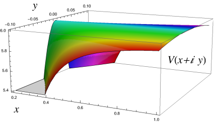
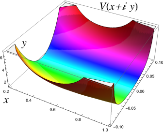
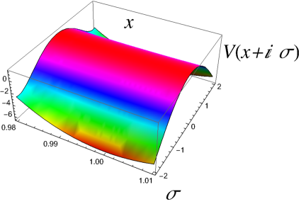
Figure 1: First row: comparison of the scalar potential, $V(\phi)$ (left) of Eq. (12), to the potential $V(\phi)$ but with $K=-3\sum_{i}^{3}\,\alpha_{i}\ln\left(\phi_{i}+\overline{\phi}_{i}+b_{i}(\phi_{i}-\overline{\phi}_{i})^{4}\right)$, Eq. (10), which stabilizes the imaginary direction. Second row: the potential $V(x+i\,\sigma)$ for $x$ and the canonical field $\sigma$. The direction $x$ gets fixed to $b$ in order to work with a canonical field, $\sigma$. For all cases we used $\alpha=1$.

It is well known that for $\alpha\leq 1$ there is an instability for any field value (e.g. [42]), while for $\alpha>1$ the non-zero eigenvalue is negative for

$$\left[\frac{\sqrt{\alpha}-1}{1+\sqrt{\alpha}}\right]^{\frac{1}{3\sqrt{\alpha}}}<\phi<\left[\frac{1+\sqrt{\alpha}}{\sqrt{\alpha}-1}\right]^{\frac{1}{3\sqrt{\alpha}}}.$$ (22)

In order to turn the imaginary component into canonical form, we need to stabilize the flat real direction. It can be done, for instance, through modifying the Kähler potential (see [43] for a review) of the model Eq. (2) by

$$K = -3\,\alpha\,\ln\left[\phi+\bar{\phi}+\,\frac{\left(\phi+\bar{\phi}-2\,b\right)^{4}}{L}\right],$$ (23)

which stabilizes the real component to $\bar{\phi}=\phi=b$, and provides a way to work only with one canonical field, $\sigma$, proportional to the imaginary direction (see Appendix A):

$$\sigma=\sqrt{\frac{3\,\alpha}{2\,b^{2}}}\,y.$$ (24)

The theory of Eq. (2) can be extended to include more fields and stabilize the real directions with the same procedure. With the addition of Eq. (23) the scalar potential has the same form of Eq. (12). Note that when fixing the real part to $b$ all the dependence inversely proportional to $L$ in Eq. (23) vanishes from the potential and their subsequent derivatives, as can be seen from Eq. (12), the form of the first derivative, Eq. (19), and of the second derivatives of $V$,

$$\partial_{i}\,\partial_{\bar{\jmath}}\,V=V_{i\,\bar{\jmath}} = e^{G}\,\left[G_{\bar{\jmath}}\left(G_{i}\,(X-3)+X_{i}\right)+G_{i\,\bar{\jmath}}(X-3)+X_{i\,\bar{\jmath}}+G_{i}\,X_{\bar{\jmath}}\right]\,,$$

$$\partial_{i}\,\partial_{j}\,V=V_{i\,j} = e^{G}\,\left[G_{j}\left(G_{i}\,(X-3)+X_{i}\right)+G_{i\,j}(X-3)+X_{ij}+G_{i}\,X_{j}\right].$$ (25)

It is clear from these expressions that up to the second derivatives in $\phi$ or $\bar{\phi}$, $G$ (e.g. $G_{ij}$) and X preserve the property of the Kähler potential in Eq. (23) to reduce to Eq. (2) when $\bar{\phi}=\phi=b$. In the third panel of Fig. 1 we compare $V$ as a function of $V(x+i\sigma)$ to the model described by Eq. (83) where the real direction has not been fixed (first panel) and to the case where the imaginary direction has been stabilized (left panel). We have chosen to plot $V(x+i\sigma)$ as we can clearly see the behaviour when $\phi=\bar{\phi}=b$. In Fig. 2 we plot the potential $V$ as a function of $\sigma$ for values of $\alpha$ which are perfect squares modulo 9, where we can see the transitions from maxima to minima: values for $\alpha\leq 1$ give de Sitter maxima, while values for $\alpha>1$ de Sitter minima.

For the case of having $\alpha=\frac{n^{2}}{9}$, $n$ an integer, using Eq. (21), then the second criterion of the RdSC, Eq. (2), can be written as $-m^{2}_{\rm Im[\phi]}/V-c^{\prime}\geq 0$ or equivalently $\left[\frac{9}{n^{2}}-1\right]b^{2n}+\left[\frac{18}{n^{2}}+2-3c^{\prime}\right]\,b^{n}+\frac{9}{n^{2}}-1\geq 0$. For $n>3$ we find that this bound can be satisfied for $b$ such that $a_{-}<b^{n}<a_{+}$ with $a_{\pm}=\frac{9+n^{2}-3c^{\prime}n^{2}/2\,\pm\,n^{2}\,\sqrt{\left(2-3c^{\prime}/2\right)\left(18/n^{2}-3c^{\prime}/2\right)}}{n^{2}-9}$ when $c^{\prime}\leq\frac{12}{n^{2}}<\frac{4}{3}$. For $n<3$ instead it can be satisfied for all values of $b$ if $\frac{4}{3}\leq c^{\prime}\leq\frac{12}{n^{2}}$. Finally for the special case $n=3$, the bound is satisfied for all values of $b$ if $c^{\prime}\leq\frac{4}{3}$.

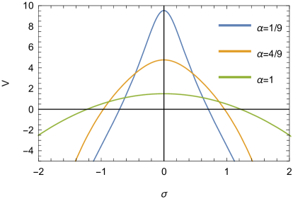
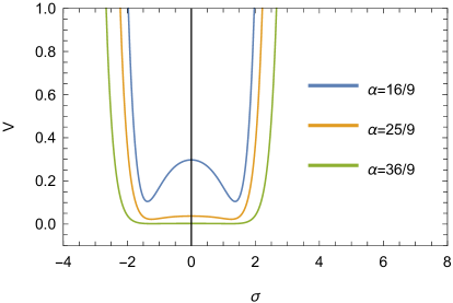
Figure 2: The scalar potential, $V(\sigma)$, of Eq. (12) with the Kähler potential of Eq. (23) with the stabilization for $\langle{\rm{Re}}\,[\phi]\rangle=b=1$, as a function of the canonical field $\sigma=\sqrt{3\,\alpha/2}\ y/b$. We have chosen values of $\alpha$ which are perfect squares modulo 9. Values for $\alpha\leq 1$, left, give de Sitter maxima, while values for $\alpha>1$, right, can admit de Sitter minima.

Trans-Planckian Conjecture in No-Scale de Sitter Models

The TCC implies that a de Sitter phase has a limited lifetime. In the case of a potential with de Sitter maximum, the field can sit on that critical point if the negative curvature, second derivative of the scalar potential, is bounded from below. Specifically, close to a local maximum if there is field range $0<\sigma<\Delta\sigma$ where $|V^{\prime\prime}|\leq|V^{\prime\prime}|_{\rm max}$, defining $V^{\prime\prime}\equiv\partial^{2}_{\sigma}V$, the TCC is satisfied if either of the following conditions are satisfied [32]

$$\Delta\sigma < \frac{\frac{2}{3\sqrt{\pi}}\left(V_{0}\,V_{\rm{min}}\right)^{3/4}\,\ln^{1/2}\sqrt{\frac{3}{V_{\rm{min}}}}}{\frac{2}{3}V(\sigma)-|V^{\prime\prime}|_{\rm{max}}\,\ln^{2}\sqrt{\frac{3}{V_{\rm{min}}}}},$$ (26)

$$\frac{|V^{\prime\prime}|_{\rm{max}}}{V_{\rm{min}}} \geq \frac{2}{3}\frac{1}{\ln^{2}\sqrt{\frac{3}{V_{\rm{min}}}}}.$$ (27)

In the above equations $|V^{\prime\prime}|_{\max}$, is the maximum curvature and $V_{\rm{min}}$ is the minimum value for the potential in that field range. The second inequality is similar to the second criterion, RdSC (2), with a prediction for $c^{\prime}$ up to a logarithmic correction and thus it is a milder constraint. For the dS no-scale model we are considering and for the single field range, the inequality Eq. (26) implies that

$$\frac{2}{3\sqrt{\pi}}\left(V_{0}V_{\rm min}\right)^{3/4}\ln^{1/2}\sqrt{\frac{3}{V_{\rm{min}}}}-\left[\frac{2}{3}V_{\rm min}-|V^{\prime\prime}|_{\rm{max}}\ln^{2}\sqrt{\frac{3}{V_{\rm{min}}}}\right]\sigma>0.$$ (28)

For $\alpha\leq 1$ the expression in the square bracket is negative and the bound is satisfied for any value of $\sigma$. In order to see that, we note $V_{\rm min}\leq V_{0}$ and $|V^{\prime\prime}|_{\rm max}\geq|V^{\prime\prime}_{0}|$, therefore

$$\frac{2}{3}V_{\rm{min}}-|V^{\prime\prime}|_{\rm max}\ln^{2}\sqrt{\frac{3}{V_{\rm{min}}}}\!\! < \!\!\frac{2}{3}V_{0}-|V^{\prime\prime}_{0}|\,\ln^{2}\sqrt{\frac{3}{V_{0}}}$$

$$= 2^{3-3\alpha}a^{2}\left[1-\frac{b^{-3\sqrt{\alpha}}}{2\alpha}\left((1+b^{3\sqrt{\alpha}})^{2}-\alpha(1-b^{3\sqrt{\alpha}})^{2}\right)\ln^{2}(2^{1-\frac{3\alpha}{2}}a)\right]\,,$$

where in the second line we have used Eq. (21) which can be written in the form

$$V^{\prime\prime}|_{\sigma=0}=-2^{2-3\alpha}a^{2}\frac{b^{-3\sqrt{\alpha}}}{\alpha}\left[(1+b^{3\sqrt{\alpha}})^{2}-\alpha(1-b^{3\sqrt{\alpha}})^{2}\right].$$ (30)

For $\alpha<1$ the above expression is negative for values of $b$ that make the potential unstable. For $\alpha=1$, the above expression is negative for $a<\sqrt{2}e^{\frac{-1}{\sqrt{2}}}$ or $a>\sqrt{2}e^{\frac{1}{\sqrt{2}}}$ independently of $b$, as can be seen from the left panel of  Fig. 3. We recall that for all phenomenological purposes $a\ll 1$. For $\alpha>1$, the analytical computation is involved as can be seen from the right panel of  Fig. 3. Numerical inspection then give us for this case the values of $\sigma$ and $b$ that are compatible with the TCC bound, Eq. (28).

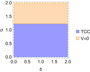
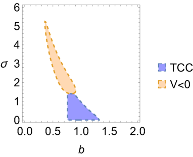
Figure 3: Evaluation of the TCC for $\alpha=1$, left plot, and $\alpha=25/9$, right plot. The blue regions indicate values of $b$ and $\sigma$ which are compatible with the TCC bound when $V>0$. The orange region indicates values for which $V<0$. For both plots we have used $a=0.1$. Note that for the case of $\alpha=1$ the value of $b$ can extend for all values along the real line.

The TCC conjecture also allows the existence of de Sitter potentials with metastable minima as long as these minima are not positive or if positive by allowing quantum tunnelling. This allows sufficiently short-lived transient quasi-dS like phases. We note that potentials with negative minima could be constructed from the kind of models of the right-side panel of Fig. 3, with addition of other fields that render the minima negative.

3 No-Scale Models with Rolling Dynamics

In this section, we first add a rolling field to our minimal model, then we obtain the conditions for finding extrema, point out in which cases there can be a stable minimum, without the addition of a quartic term in the Kähler potential. Then we point out in which cases instead we can be in agreement with the first criterion of the RdSC, Eq. (1).

Following the approach proposed in [44], we modify the Kähler potential and the superpotential of our basic dS no-scale model as follows

$$\widehat{K} = K-\sum_{m=1}^{N}\,q_{m}\ln(\chi_{m}+\bar{\chi}_{m}),$$ (31)

$$\widehat{W} = W\,\prod_{m=1}^{M}\,\left(c_{0,m}+c_{1,m}\,\chi_{m}^{-{\nicefrac{{p_{m,1}}}{{2}}}}+c^{2}_{m}\,\chi_{m}^{-{\nicefrac{{p_{m,2}}}{{2}}}}+\cdots\right).$$ (32)

Here $m$ runs over the number of rolling chiral superfields, $q_{m}>0$, $c_{k,m}$ are arbitrary constants and the powers $p_{m,k}$ satisfy $p_{m,k}<0$. The function invariant under Kähler transformations $\widehat{G}=\widehat{K}+\ln\ \left|\widehat{W}\right|^{2}$ of the modified model is given by

$$\widehat{G}=G+\sum_{m=1}^{M}\,\left(\ln\frac{|c^{0}_{m}+c^{1}_{m}\,\chi_{m}^{-{\nicefrac{{p_{m}^{1}}}{{2}}}}+c^{2}_{m}\,\chi_{m}^{-{\nicefrac{{p_{m}^{2}}}{{2}}}}+\cdots|^{2}}{(\chi_{m}+\bar{\chi}_{m})^{q_{m}}}\right)\equiv G+\widetilde{G},$$ (33)

where additional chiral superfields $\chi_{m}$ are included to provide an escape to the RdSC for positive scalar potentials, Eq. (4). The addition of these chiral superfields solves at the same time the instability of $K$ at Im $\phi$=0, for which V has a maximum, Eq. (5) without additional quartic terms. The scalar potential for this model can be written then as follows

$$\widehat{V} = e^{\widehat{G}}\left(\sum_{I=1,\bar{J}=1}^{N+M,N+M}\widehat{G}_{I}\,\widehat{K}^{I\bar{J}}\,\widehat{G}_{\bar{J}}-3\right)$$ (34)

$$= e^{\widehat{G}}\left(\sum_{i=1,\bar{\jmath}=1}^{N,N}\widehat{G}_{i}\,\widehat{K}^{i\bar{\jmath}}\,\widehat{G}_{\bar{\jmath}}-3\right)+e^{\widehat{G}}\left(\sum_{m=1,\bar{n}=1}^{M,M}\widehat{G}_{m}\,\widehat{K}^{m\bar{n}}\,\widehat{G}_{\bar{n}}\right)$$

$$= e^{\widetilde{G}}\,\left(V+\widehat{X}\,{\rm{e}}^{G}\right),$$

where $I=i,m$ runs over all chiral superfields, indices $i,j=1,\ldots,N$ are for the de Sitter fields, indices $m,n=1,\ldots,M$ are devoted to the rolling fields, $\widehat{K}^{I\bar{J}}$ is the inverse of the Kähler metric (which is block diagonal) $\widehat{K}_{I\bar{J}}=\partial_{I}\partial_{\bar{J}}\,\widehat{K}$ and $\widehat{G}_{I}=\partial_{I}\,\widehat{G}$, analogously for its Hermitian conjugate. The parameter $\widehat{X}$ is defined as

$$\widehat{X}\equiv\widehat{G}_{m}\,\widehat{K}^{m\bar{n}}\,\widehat{G}_{\bar{n}}=\widetilde{G}_{m}\,\widehat{K}^{m\bar{n}}\,\widetilde{G}_{\bar{n}},$$ (35)

where the expression after the equal sign follows from the decomposition in Eq. (33) and $\widehat{G}_{m}=\widetilde{G}_{m}$ since only $\widetilde{G}$ depends on the “rolling” fields $\chi$. For the rest of this section we assume just one rolling field $\chi$. The potential $\widehat{V}$ is minimal in the $\chi$ plane for $\rm{Im}\,[\chi]=0$, therefore we consider only the real part of the scalar field

$$\gamma=\left.\widehat{X}\right|_{\widehat{V}_{\rm{Re}\,[\chi]}}.$$ (36)

The extremization condition of the new scalar potential, $\widehat{V}$, is

$$\partial_{i}\,\widehat{V}=e^{\widetilde{G}}\,\left(\partial_{i}\,V+\gamma\ \partial_{i}\,e^{G}\right)=e^{\widetilde{G}}\,\left(\partial_{i}\,V+\gamma\ \partial_{i}\,(e^{K}|W|^{2})\right)=0.$$ (37)

This equation can be satisfied in two ways. One way is requiring both terms to cancel independently, since $\partial_{\bar{i}}V=0$ and $\partial_{\bar{\imath}}\,V=0$ are the conditions for the minimum of the original theory this can be easily satisfied and hence the term $\partial_{i}\,(e^{K}|W|^{2})$ should be satisfied independently. The other way is to achieve a cancellation with both terms.

In the case of finding solutions where $W=0$, the solutions for $\partial_{i}\,V$, Eq. (18), can be written as follows

$$\partial_{i}\,V=e^{K}\,\overline{W}_{\bar{\jmath}}\left[K^{\bar{\jmath}l}\left(W_{l}\,K_{i}+W_{i}\,K_{l}+W_{li}\right)+K^{\bar{\jmath}l}\,_{i}W_{l}\right]=0.$$ (38)

When the addition of the rolling field does not change the minima of the no-scale field in the supersymmetry breaking vacuum, then the no-scale field is stabilized and the only dynamics comes from the rolling field, as it has been emphasized in [44]. For the second term in Eq. (37) we have

$$\partial_{i}\left(e^{K}|W|^{2}\right)=e^{K}\ \overline{W}\left(WK_{i}+W_{i}\right),$$ (39)

for which we have two solutions for a vanishing term

$$W=0\quad\text{or}\quad D_{i}\,W=K_{i}+\frac{W_{i}}{W}=0,$$ (40)

analogously for their hermitian counterparts. The first solution in Eq. (40) can be satisfied in general, while the second solution just holds for certain values of $\alpha$. We choose the first one, so we have at the extrema

$$\prod_{i=1}^{N}\,\phi_{i}^{n_{i+}} = \prod_{i=1}^{N}\,\phi_{i}^{n_{i-}},$$

$$\prod_{i=1}^{N}\,\overline{\phi}_{i}^{n_{i+}} = \prod_{i=1}^{N}\,,\overline{\phi}_{i}^{n_{i-}},$$ (41)

where non trivial solutions (for which $n_{i+}\neq n_{i-}$) exist, as we will see in the next sections, hence

$$\left.\partial_{\bar{\imath}}\left(e^{K}|W|^{2}\right)\right|_{\prod_{i=1}^{N}\,\overline{\phi}_{i}^{n_{i}+}=\prod_{i=1}^{N}\,\overline{\phi}_{i}^{n_{i}-}}=0,$$ (42)

$$\left.\partial_{i}\left(e^{K}|W|^{2}\right)\right|_{\prod_{i=1}^{N}\,\phi_{i}^{n_{i}+}=\prod_{i=1}^{N}\,\phi_{i}^{n_{i}-}}=0.$$

Finally, we note that the evaluation of $\widehat{V}$ at the extrema for the no-scale fields implies

$$\left.\ \frac{K^{I\bar{J}}\,\partial_{I}\widehat{V}\,\partial_{\bar{J}}\,\widehat{V}}{\widehat{V}^{2}}=\ \frac{\widehat{K}^{m\bar{n}}\partial_{m}\,\widehat{V}\partial_{\bar{n}}\,\widehat{V}}{\widehat{V}^{2}}\right|_{\rm{\widehat{V}_{\rm{ext.}}}}=\gamma\,,$$ (43)

where we have used $\partial_{i}\,\widehat{V}=0$. We observe that the rolling behavior in this no-scale supergravity puts the model out of the swamp given that $2\gamma\geq c^{2}$. It is interesting to note, as the superpotential is vanishing in the vacuum, that we get a supersymmetry breaking vacuum with positive vacuum energy for any value of $\gamma$. This can be seen by expanding the scalar potential $\widehat{V}$ into pieces of the original model and the pieces coming from the rolling field

$$\widehat{V}={e}^{\widetilde{G}}\,{e}^{K}|W|^{2}\,\left(X-3+\gamma\right)={e}^{\widetilde{G}}\,e^{K}\,\left(\sum_{i=1}^{N}\,\left|D_{i}\,W\right|^{2}+(\gamma-3)|W|^{2}\right),$$ (44)

from which it follows that at the extrema of the complete model the dependence on $\gamma$ disappears when $W=0$

$$\widehat{V}=\left.e^{\widetilde{G}}\,\left(\,e^{K}\,\sum_{i=1}^{N}\,|D_{i}\,W|^{2}\,\right)\right|_{\rm ext.}.$$ (45)

The Minimal Model

In this section we study the minimal model including a no-scale chiral superfield plus a rolling superfield.

Existence of Extrema

We start with the simplest example including one no-scale chiral superfield and one rolling chiral superfield. The Kähler and the superpotential are as follows

$$\widehat{K} = -3\,\alpha\,\ln(\phi+\bar{\phi})-q\,\ln(\chi+\bar{\chi}),$$

$$\widehat{W} = a\left(\phi^{n_{+}}-\phi^{n_{-}}\right)\,\chi^{-p/2},$$ (46)

where $\alpha,q>0,p<0$, $a$ is an arbitrary constant and $n_{\pm}=3/2(\alpha\pm\sqrt{\alpha})$. The full scalar potential, $\widehat{V}$, is as in Eq. (34), $V$, the no-scale potential is given in Eq. (12) and $\widetilde{G}$ is

$${\widetilde{G}} = \ln\left[({2\rm Re}\,[\chi])^{-q}\,|\chi|^{-p}\right],$$ (47)

For the second term Eq. (37) the extremization conditions of Eq. (42), for the non-trivial solution (that is $n_{i-}\neq n_{i+}$), and for an arbitrary value of $\alpha$ reduce to

$$\left.\phi\right|_{\rm ext.}=\left.\bar{\phi}\right|_{\rm ext.}=1,$$ (48)

which is in agreement with the condition for finding the extrema of the original theory, Eq. (20), but restricts the set of possible values for the extrema. If we instead consider the Kähler potential of Eq. (23), this can automatically fix $\phi=\bar{\phi}=1$ by choosing $b=1$ as explained in section 2.

Stability Condition

We study the stability of the vacuum by considering the Hessian matrix

$$\mathcal{H}=\left[\begin{array}[]{ll}K^{J\bar{L}}\,\nabla_{I}\nabla_{\bar{L}}\widehat{V}&K^{L\overline{M}}\,g_{\overline{M}I}\,\nabla_{L}\nabla_{J}\widehat{V}\\[10.0pt] K^{I\bar{L}}\,g^{J\overline{M}}\,\nabla_{\bar{L}}\nabla_{\overline{M}}\,\widehat{V}&K^{I\bar{L}}\,\nabla_{\bar{L}}\nabla_{J}\widehat{V}\,,\end{array}\right]\,,$$ (51)

where $I=\phi,\chi$ and $\widehat{V}_{IJ}=\nabla_{I}\,\nabla_{J}\,\widehat{V}=\partial_{I}\,\partial_{J}\widehat{V}-\Gamma^{K}_{IJ}\,\partial_{K}\,\widehat{V}$. For the no-scale extremization where $\partial_{\phi}V=0$ and $e^{G}\sim|W|^{2}=0$ we find that

$$\left.\widehat{V}_{\phi\chi}\,\right|_{\rm min}=\left(\partial_{\chi}\,e^{\widetilde{G}}\right)\,\left(\partial_{\phi}V\right)+\gamma\,e^{\widetilde{G}}\,e^{G}(G_{\phi}\,G_{\chi})=0,$$ (52)

similarly for any other mixed component and its Hermitian conjugate. The no-scale components do not mix with the rolling field, thus the mixed Christoffel symbols are vanishing. Therefore, we can write the Hessian matrix as

$$\left.{\mathcal{H}}\right|_{\phi=\bar{\phi}=1}=\left.\begin{bmatrix}\widehat{K}^{\phi\bar{\phi}}\,\widehat{V}_{\phi\bar{\phi}}&0&\widehat{K}^{\phi\bar{\phi}}\,g_{\bar{\phi}\phi}\,\widehat{V}_{\phi\phi}&0\\ 0&\widehat{K}^{\chi\bar{\chi}}\,\widehat{V}_{\chi\bar{\chi}}&0&\widehat{K}^{\chi\bar{\chi}}\,g_{\bar{\chi}\chi}\,\widehat{V}_{\chi\chi}\\ \widehat{K}^{\phi\bar{\phi}}\,g^{\bar{\phi}\phi}\,\widehat{V}_{\bar{\phi}\bar{\phi}}&0&\widehat{K}^{\phi\bar{\phi}}\widehat{V}_{\bar{\phi}\phi}&0\\ 0&\widehat{K}^{\chi\bar{\chi}}\,g^{\bar{\chi}\chi}\,\widehat{V}_{\bar{\chi}\bar{\chi}}&0&\widehat{K}^{\chi\bar{\chi}}\,\widehat{V}_{\bar{\chi}\chi}\end{bmatrix}\right|_{\phi=\bar{\phi}=1},$$ (53)

from which we can see that it is equivalent to look for the eigenvalues, which need to be positive for the stability of the scalar potential, of the following block-diagonal matrix

$${\mathcal{H}}=\left[\begin{array}[]{cc}\mathcal{H}_{\phi}&0\\ 0&\mathcal{H}_{\chi}\end{array}\right].$$ (56)

Each of the blocks in Eq. (56) contain only information from one field:

$$\rm{det}\left[\mathcal{H}_{\phi}\right]=\rm{det}\left[K^{\phi\bar{\phi}}\,\begin{bmatrix}\widehat{V}_{\phi\bar{\phi}}&\widehat{V}_{\phi\phi}\\ \widehat{V}_{\bar{\phi}\bar{\phi}}&\widehat{V}_{\bar{\phi}\phi}\end{bmatrix}\right],\quad\rm{det}\left[\mathcal{H}_{\chi}\right]=\rm{det}\left[K^{\chi\bar{\chi}}\,\begin{bmatrix}\widehat{V}_{\chi\bar{\chi}}&\widehat{V}_{\chi\chi}\\ \widehat{V}_{\bar{\chi}\bar{\chi}}&\widehat{V}_{\bar{\chi}\chi}\end{bmatrix}\right],$$ (57)

also, due to having only one field in each sector, and $\widehat{K}^{\phi\bar{\phi}}=K^{\phi\bar{\phi}}$, $\widehat{K}^{\chi\bar{\chi}}=K^{\chi\bar{\chi}}$, the factor of the Kähler metric factors out. We therefore can look independently for the eigenvalues of the sub-matrices $\mathcal{H}_{\phi}$ and $\mathcal{H}_{\chi}$. The second derivatives of the scalar potential, Eq. (34), at the local extrema are given as follows

$$\widehat{V}_{\phi\phi} = e^{\widetilde{G}}\,\left(\partial_{\phi}\,\partial_{\phi}V\right)+\gamma\,e^{\widehat{G}}\,\left(K_{\phi\phi}+G_{\phi}G_{\phi}\right)-\Gamma^{\phi}_{\phi\phi}\,\partial_{\phi}\widehat{V}=e^{\widetilde{G}}\left(2^{-3\alpha}\,\times 6\,a^{2}\right),$$

$$\widehat{V}_{\phi\bar{\phi}} = e^{\widetilde{G}}\,\left(\partial_{\phi}\,\partial_{\bar{\phi}}V\right)+\gamma\,e^{\widehat{G}}\,(K_{\phi\bar{\phi}}+G_{\phi}G_{\bar{\phi}})=e^{\widetilde{G}}\left(-2^{-3\alpha}\,\times 6\,a^{2}+2^{-3\alpha}\,\times 9\,\gamma\,\alpha\,a^{2}\right),$$

$$\widehat{V}_{\bar{\phi}\bar{\phi}} = e^{\widetilde{G}}\,\left(\partial_{\bar{\phi}}\,\partial_{\bar{\phi}}V\right)+\gamma\,e^{\widehat{G}}\,(K_{\bar{\phi}\bar{\phi}}+G_{\bar{\phi}}G_{\bar{\phi}})-\Gamma^{\bar{\phi}}_{\bar{\phi}\bar{\phi}}\,\partial_{\bar{\phi}}\widehat{V}=e^{\widetilde{G}}\left(2^{-3\alpha}\,\times 6\,a^{2}\right),$$ (58)

where $e^{\widetilde{G}}$ is given in Eq. (47) and the Christoffel symbols in Eq. (17). We note that $e^{\widehat{G}}\,G_{\phi}\,G_{\bar{\phi}}\neq 0$. Finally, the eigenvalues of the Hessian $\mathcal{H}_{\phi}$ at $\phi=\bar{\phi}$ are

$$\lambda_{1} = \text{e}^{\widetilde{G}}\,\frac{4}{3\,\alpha}\,\left[9\,\times 2^{-3\,\alpha}\,a^{2}\,\alpha\,\gamma\right]=3\times\text{e}^{\widetilde{G}}\times 2^{2-3\,\alpha}\,a^{2}\,\gamma,$$

$$\lambda_{2} = \text{e}^{\widetilde{G}}\,\frac{4}{3\,\alpha}\,\left[3\,\times 2^{-3\,\alpha}\,a^{2}(-4+3\,\alpha\gamma)\right]=\text{e}^{\widetilde{G}}\times 2^{2-3\,\alpha}\,a^{2}\left(-\frac{4}{\alpha}+3\,\gamma\right).$$ (59)

Therefore, the stability condition for having a de Sitter minimum implies

$$3\,\alpha\,\gamma>4.$$ (60)

This shows that adding a rolling dynamics, without adding a quartic term in the Kähler metric to stabilize the imaginary part, Eq. (10), also provides a way to stabilize the potential. In case presented in this section, the eigenvalues of $\lambda_{1}$ and $\lambda_{2}$, Eq. (3) can be both positive for suitable values of $\alpha$ and $\gamma$.

Assertion of the Refined de Sitter Conjecture

Now we check whether the modified no-scale model obeys the first criterion of RdSC, Eq. (1), or not. We first compute the parameter $\gamma$, from Eq. (35)

$$\gamma=\left.G_{\chi}\,K^{\chi\bar{\chi}}\,G_{\bar{\chi}}\right|_{{\rm Im}\chi=0}=\left.\frac{1}{q|\chi|^{2}}\left[q^{2}|\chi|^{2}+\left(\frac{p}{2}\right)^{2}\ |\chi+\overline{\chi}|^{2}+q\ p\left(\chi+\overline{\chi}\right)^{2}\right]\right|_{{\rm Im}\chi=0}=\frac{(p+q)^{2}}{q},$$ (61)

where

$$G_{\chi}=-\frac{p}{2\chi}-\frac{q}{\chi+\bar{\chi}},\quad{\rm and}\quad G_{\bar{\chi}}=-\frac{p}{2\bar{\chi}}-\frac{q}{\chi+\bar{\chi}},$$ (62)

and $K^{\chi\bar{\chi}}$ is the inverse of the Kähler metric

$$K_{\chi\bar{\chi}}=\frac{q}{(\chi+\bar{\chi})^{2}}.$$ (63)

The first criterion of RdSC, Eq. (1), in the form of Eq. (4), is satisfied if

$$\frac{\sqrt{2}(p+q)}{\sqrt{q}}\geq c={\cal O}(1).$$ (64)

Along the real direction, we have

$$e^{\widetilde{G}}=|\chi\,\bar{\chi}|^{-p/2}(\chi+\bar{\chi})^{-q}=({\rm Re}\,\chi)^{-(p+q)}=e^{\sqrt{2\gamma}\,\chi^{c}},$$ (65)

where $\chi^{c}$ is the canonically normalized rolling scalar field. Finally, we note that if the first criterion is violated, the second criterion of the RdSC, Eq. (2), can be satisfied if there is an instability. In fact, the second mass eigenvalue is negative for $3\,\alpha\,\gamma<4$. Given that $\widehat{V}=12\,a^{2}\,\times 2^{-3\,\alpha}e^{\sqrt{2\,\gamma}\,\chi^{c}}$ in the real field direction, the second criterion of the RdSC, Eq. (2), requires that

$$3\,\alpha\,\gamma\leq 4-\alpha\,c^{\prime}.$$ (66)

Since we computed the Hessian for non-canonical fields, but kept the Kähler metric in Eq. (51) we can evaluate the second criterion, Eq. (2), involving the fields $\phi$ and $\chi$, without the need of using canonical fields.

Superpotential with two Terms in the Expansion of the Rolling Field

Now we modify the superpotential Eq. (3) of the minimal model to take the following form

$$W=(\phi^{n_{+}}-\phi^{n_{-}})(a_{1}\,\chi^{-p_{1}/2}+a_{2}\,\chi^{-p_{2}/2}).$$ (67)

From Eq. (33) we compute

$$e^{\widetilde{G}}=(\chi+\bar{\chi})^{-q}\,\left|a_{1}\chi^{-p_{1}/2}+a_{2}\,\chi^{-p_{2}/2}\right|^{2},$$ (68)

where

$$G_{\chi}=-\frac{p_{1}+q}{2\,\chi}-\frac{(p_{2}-p_{1})\,a_{2}}{2\,\chi(a_{1}\,\chi^{(p_{2}-p_{1})/2}+a_{2})},$$ (69)

to finally get

$$\gamma=\frac{(p_{1}+q)^{2}}{q}+\frac{a_{2}\,(p_{2}-p_{1})}{q}\left[\frac{a_{2}\,(p_{2}-p_{1})}{a_{1}\,\chi^{(p_{2}-p_{1})/2}+a_{2}}+2(p_{1}+q)\right]\frac{1}{a_{1}\,\chi^{(p_{2}-p_{1})/2}+a_{2}}.$$ (70)

From Eq. (70) we observe that as far as $\sqrt{2\gamma}\geq c$ the RdSC, in the form of Eq. (4), can be satisfied.

4 Non-minimal No-Scale Models

2+1 Model

Next, we consider a no-scale supergravity with dS vacuum generated by two chiral superfields $\phi_{i}$ and add one rolling superfield $\chi$, we refer to this construction as the 2+1 Model. The Kähler and the superpotential are as follows

$$K = -3\,\alpha_{1}\ln(\phi_{1}+\bar{\phi}_{1})-3\,\alpha_{2}\,\ln(\phi_{2}+\bar{\phi}_{2})-q\,\ln(\chi+\bar{\chi}),$$ (71)

$$W = a\left(\phi_{1}^{n_{1+}}\,\phi_{2}^{n_{2+}}-\phi_{1}^{n_{1-}}\,\phi_{2}^{n_{2-}}\right)\,\chi^{-p/2},$$ (72)

where $\alpha_{i},q>0,p<0$, $a$ is an arbitrary constant and $n_{i\pm}$ are given in Eq. (7). From Eq. (3) and demanding $n_{i+}\neq n_{i-}$, we have

$$\phi_{1}^{r_{1}}\phi_{2}^{r_{2}}=\bar{\phi}_{1}^{r_{1}}\bar{\phi}_{2}^{r_{2}}=1,$$ (73)

where $r_{1},r_{2}$ are arbitrary constants satisfying $r_{1}^{2}+r_{2}^{2}=1$. We note that we cannot have both $\partial_{1}\,W$ and $\partial_{2}\,W$ simultaneously vanishing as supersymmetry is spontaneously broken and the scalar potential is lifted. However, one of them can vanish for special case of $r_{1}=0$ and $r_{2}=1$, or vice versa. Moreover, we observe that the above solution Eq. (73) satisfies Eq. (38). Similar to the minimal model, the Hessian matrix can be brought to a block diagonal form, Eq. (56), where now

$${\mathcal{H}}_{\phi}=\left[\begin{array}[]{cccc}K^{1\bar{1}}\,\widehat{V}_{1\bar{1}}&K^{1\bar{1}}\,g_{1\bar{1}}\,\widehat{V}_{11}&K^{1\bar{1}}\,\widehat{V}_{1\bar{2}}&K^{1\bar{1}}\,g_{1\bar{1}}\widehat{V}_{12}\\ K^{1\bar{1}}\,g^{1\bar{1}}\widehat{V}_{\bar{1}\bar{1}}&K^{1\bar{1}}\,\widehat{V}_{\bar{1}1}&K^{1\bar{1}}\,g^{1\bar{1}}\,\widehat{V}_{\bar{1}\bar{2}}&K^{1\bar{1}}\,\widehat{V}_{\bar{1}2}\\ K^{2\bar{2}}\,g^{2\bar{2}}\,\widehat{V}_{2\bar{1}}&K^{2\bar{2}}\,g_{2\bar{2}}\,\widehat{V}_{21}&K^{2\bar{2}}\widehat{V}_{2\bar{2}}&K^{2\bar{2}}\,g_{2\bar{2}}\,\widehat{V}_{22}\\ K^{2\bar{2}}\,g^{2\bar{2}}\,\widehat{V}_{\bar{2}\bar{1}}&K^{2\bar{2}}\,\widehat{V}_{\bar{2}1}&K^{2\bar{2}}\,\,g^{2\bar{2}}\widehat{V}_{\bar{2}\bar{2}}&K^{2\bar{2}}\,\widehat{V}_{\bar{2}2}\end{array}\right],$$ (78)

and ${\mathcal{H}}_{\chi}$ is as in Eq. (57), therefore the problem reduces to analyzing the $4\times 4$ ${\mathcal{H}}_{1}$ matrix of Eq. (78). Analogously to Eq. (3) we need to compute the second order derivatives of $\widehat{V}$ with respect to $\phi_{1}$ and $\phi_{2}$: $\widehat{V}_{\phi_{i}\phi_{j}}=\partial_{i}\,\partial_{j}\,{\rm{e}}^{\widetilde{G}}\left(V+\gamma\,e^{G}\right)=$ ${\rm{e}}^{\widetilde{G}}\,\partial_{i}\,\partial_{j}\,\left(V+\gamma\,e^{G}\right)$. These derivatives are given in the Appendix B. We find that the eigenvalues are given as follows

$$\lambda_{1}=0,$$

$${e^{-\tilde{G}}} \lambda_{2}=\frac{12\,\times 2^{-3\,(\alpha_{1}+\alpha_{2})}a^{2}(3\,r_{2}^{2}\,\alpha_{1}+3\,r_{1}^{2}\,\alpha_{2}+s^{2}\,\alpha_{1}\,\alpha_{2}(\gamma-3))(r_{2}^{2}\alpha_{1}+r_{1}^{2}\alpha_{2})}{s^{4}\,\alpha_{1}^{2}\,\alpha_{2}^{2}},$$ (79)

where $s$ has been defined in Eq. (7) , which requires

$$3\,r_{2}^{2}\,\alpha_{1}+3\,r_{1}^{2}\,\alpha_{2}+s^{2}\,\alpha_{1}\,\alpha_{2}(\gamma-3)>0,$$ (80)

while the other two eigenvalues are of the form

$${e^{-\tilde{G}}}\,\lambda_{\pm}=A\pm\sqrt{B},$$ (81)

where $A$ and $B$ are independent of $\phi_{1}$ and $\phi_{2}$. In Fig. 4 we plot the possible values of $\alpha_{1}$ and $\alpha_{2}$ for the special case of $\gamma=2$ and $c^{\prime}=1$ with $r_{1}=r_{2}=\frac{1}{\sqrt{2}}$ that are compatible either with the RdSC or the stability condition.

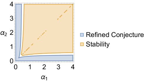
Figure 4: Parameter space of $\alpha_{1}$ and $\alpha_{2}$, for the $2+1$ model for the special case of $\gamma=2$ and $c^{\prime}=1$ with $r_{1}=r_{2}=\frac{1}{\sqrt{2}}$, that can be either compatible with the RdSC or the stability condition.

N+1 Model

We generalize to the case of N de Sitter case plus a rolling field with the following general Kähler potential and superpotential

$$K = -3\sum_{i=1}^{N}\alpha_{i}\ln(\phi_{i}+\bar{\phi}_{i})-q\ln(\chi+\bar{\chi})=K-q\ln(\chi+\bar{\chi}),$$ (82)

$$W = a\,\left(\prod_{i=1}^{N}\phi_{i}^{n_{i+}}-\prod_{i=1}^{N}\phi_{i}^{n_{i-}}\right)\,\chi^{-p/2}=W\chi^{-p/2}.$$ (83)

In this case, local supersymmetry breaking vacua exist when for some fields Eq. (3) is satisfied (leading to $W=\overline{W}=0$), which can be put in the form

$$\prod_{i=1}^{N}\phi_{i}^{r_{i}}=\prod_{i=1}^{N}\bar{\phi}_{i}^{r_{i}}=1,$$ (84)

where $r_{1},r_{2}$ are arbitrary constants satisfying $\sum_{i=1}^{N}r_{i}^{2}=1$. We note that we cannot have $\partial_{i}\,W$ simultaneously vanishing for all $i$. However, some of them can vanish for special values of $r_{i}$. As with the previous examples this solution automatically satisfies $\partial_{i}\,V=0$, Eq. (38), which requires $\phi=\bar{\phi}$. The part of the Hessian regarding only $\phi_{i}$ fields does not mix with that of $\chi_{i}$, hence as in the previous case the total Hessian is block diagonal, Eq. (56), where

$${\mathcal{H}}_{\phi}=\left[\begin{array}[]{ccccc}\widehat{V}_{\phi_{1}\bar{\phi}_{1}}&\widehat{V}_{\phi_{1}\bar{\phi}_{2}}&\ldots&\ldots&\widehat{V}_{\phi_{1}\phi_{N}}\\ \widehat{V}_{\phi_{2}\bar{\phi}_{1}}&\widehat{V}_{\phi_{2}\bar{\phi}_{2}}&\ldots&\ldots&\widehat{V}_{\phi_{2}\phi_{N}}\\ \vdots&\vdots&\vdots&\vdots&\vdots\\ \widehat{V}_{\bar{\phi}_{N}\phi_{1}}&\ldots&\ldots&\ldots&\widehat{V}_{\bar{\phi}_{N}\phi_{N}}\end{array}\right],$$ (89)

and ${\mathcal{H}}_{\chi}$ is as in Eq. (57), therefore the problem reduces to analysing the $2\,N\times 2\,N$ ${\mathcal{H}}_{\phi}$ matrix, which in principle is not block diagonal itself.

5 Application to Quintessence Models

Current data indicates that the universe is dominated by dark energy, therefore if Eq. (1) is satisfied, this implies that this cannot be the result of a positive cosmological constant nor can be described by a state at the minimum of a potential with positive energy density. In such a case we can invoke Quintessence models, which are described by rolling fields. It is known that exponential potentials of the form $V=V_{0}\,e^{\lambda\,\chi}$ [45] and

$$V(\chi)=V_{1}\,e^{\lambda_{1}\,\chi}\,+\,V_{2}\,e^{\lambda_{1}\,\chi},$$ (90)

with varying $\lambda_{i}$ parameters [49] that can fit well the constraints based on Supernovae type Ia (SNeIa), Cosmic Microwave Background (CMB) and Baryon Acoustic Oscillations (BAO) data (see [50] for an alternative conclusion). For the case of one rolling field $\chi$, and hence only one term in Eq. (90), $V(\chi)=V_{1}\,e^{\lambda\,\chi}$, the variable $\lambda$ is constrained to be $\lambda=c$, which is the constant appearing in Eq. (1), and must satisfy $\lambda\lesssim 0.6$. In [44] the mechanism that we use in this work to satisfy the RdSC was applied to uplift a vacuum to a de Sitter vaccum that could be in agreement with the RdSC but it was concluded that the breaking of supersymmetry needed for the de Sitter uplift cannot be only caused by the Quintessence field $\chi$ due to the requirement $\gamma=c>3$. In the models we present in section 3 we do not have such a requirement and hence even our minimal model with one rolling field plus one de Sitter field could be used as a Quintessence model. In particular our result for the minimal model for the constraint on $\gamma$ is compatible with a value of $0.6$.

The potential with two terms, Eq. (90), is in fact a kind of freezing model associated with scaling solutions [51], where the field equation of state scales as that of the background fluid during most of the matter era. Here the constants $\lambda_{i}$ are constrained to $\lambda_{1}\gg 1$ and $\lambda_{2}\lesssim 1$ [49]. In the early matter era, the potential is approximated by the first term in Eq. (90) while at late times the second term. In [45] it was shown that the potential of Eq. (90) with $\lambda\approx\lambda_{1}>>\sqrt{3}$ in the early universe and then switches to $\lambda\approx\lambda_{2}=c=0.6$ at some recent point in the past. Together these two stages approxiate the boundary trajectory that the dark energy equation of state, $\omega(a)=\omega_{0}+\omega_{a}(1-a)$, where $a$ is the scale factor normalized as $a=1$ today, needs to satisfy in order to be in agreement with SNeIa, CMB and BAO and the RdSC, Eq. (1), as shown in [45]. The No-Scale models that we study in section 3 can easily accommodate these requirements. We are aware about the difficulties in constructing Quintessence models in supergravity [52], where either it is difficult to evade gravitational tests or having the Quintessence/supegravity models behave like pure cosmological constants. Nevertheless, our result is encouraging from the viewpoint of making compatible a supergravity theory with the Refined de Sitter conjecture .

6 Conclusions

In this paper, we used the Refined de Sitter Conjecture (RdSC) and the Trans-Planckian Censorship Conjecture (TCC) to constrain the parameter space of some no-scale supergravity models. Specifically, we have studied a toy model of one field with no-scale Kähler potential and a superpotential constructed from two Minkowski endpoints, which yields a de Sitter scalar potential. It is well known that for a particular choice of parameters, this model is unstable along the imaginary direction, that is the second derivative of the scalar potential is negative. But this is exactly the kind of model that the RdSC allows and the TCC can constrain. To check the compatibility with the RdSC and the TCC we first added a quartic term to the original Kähler potential to stabilize the real part of the field, allowing us to work with one canonical field that is proportional to the imaginary direction. Using this, we have shown that for some choices of parameters the theory can be compatible with the RdSC and the TCC. This analysis can be extended to the case of multi-field theories as well as to cases with meta-stable de Sitter vacua, where the imaginary direction can also be modified via a quartic term in the Kähler potential. We think this kind of analysis is important as no-scale models with Minkowski/Anti-de Sitter vacua generically appear as low energy limits of string compactifications, but de Sitter vacua “have not yet been rigorously shown to be realized in string theory” [30].

To construct the second class of models we presented in this paper, for which an effective dS background is obtained from a rolling potential, we modified the Kähler and superpotential of the simplest no-scale model we considered by adding the terms corresponding to the rolling fields. We found that this modification alleviates the instability and flatness along the imaginary and the real directions without the need for quartic terms. The existence of the rolling direction provides an escape from the swamp as the first criterion of the RdSC can be satisfied for suitable values of parameters. Interestingly, we found that the height of the potential is controlled by the no-scale parameters while the rolling parameters make the model compatible with the RdSC. These models could be used to construct viable cosmological models to accommodate the accelerating expansion of the late Universe.

Appendix A Canonical Normalization

To evaluate the second criterion of the RdSC, Eq. (2), we split the complex field $\phi$ into real and imaginary components $\phi=x+iy$, to have

$${\mathcal{L}}=-K_{\phi\bar{\phi}}\,\partial_{\mu}\phi\,\partial^{\mu}\bar{\phi}=-\,\frac{3\alpha}{4\,[{\rm{Re}}[\phi]]^{2}}\,\left[(\partial_{\mu}x)(\partial^{\mu}x)+(\partial_{\mu}y)(\partial^{\mu}y)\right].$$ (91)

With the Kähler metric of Eq. (23) we can fix the real part to b, such that

$$\langle{\rm{Re}}[\phi]\rangle=b.$$ (92)

Then we identify the canonical kinetic term of the fields $\chi$ and $\sigma$:

$${\mathcal{L}}=-\left(\frac{1}{\sqrt{2}}\partial_{\mu}\chi\right)^{2}-\left(\frac{1}{\sqrt{2}}\partial_{\mu}\sigma\right)^{2},$$ (93)

we would have

$$\frac{1}{\sqrt{2}}\,\partial_{\mu}\chi=\sqrt{\frac{3\alpha}{4\,[{\rm{Re}}[\phi]]^{2}}}\,\partial_{\mu}x\,,$$ (94)

$$\frac{1}{\sqrt{2}}\,\partial_{\mu}\sigma=\sqrt{\frac{3\alpha}{4\,}}\,\frac{\partial_{\mu}y}{b}\,\rightarrow\,\sigma=\sqrt{\frac{3\alpha}{2}}\,\frac{y}{b}.$$ (95)

But since the real part is fixed and acquires a vev, then our effective theory will consist in only one field, $\sigma$, with canonical kinetic term ${\mathcal{L}}=-\frac{1}{2}\,\partial_{\mu}\sigma\partial^{\mu}\sigma$.

Appendix B Details of Stability Conditions

For the 2+1 Model the second derivatives of $\widehat{V}$ are as follows

$$\frac{1}{e^{\widetilde{G}}}K^{1}_{1}\widehat{V}^{1}_{\;\;1} = \frac{1}{e^{\widetilde{G}}}K^{1}_{1}\widehat{V}_{1}^{\;1}=\frac{4\,\times 2^{-3\,(\alpha_{1}+\alpha_{2})}a^{2}(3r_{2}^{2}\alpha_{1}^{2}-2r_{1}^{2}\alpha_{2}+3\,\gamma\alpha_{1}\alpha_{2}r_{1}^{2})}{s^{2}\alpha_{1}^{2}\alpha_{2}},$$

$$\frac{1}{e^{\widetilde{G}}}K^{1}_{1}\widehat{V}^{11} = \frac{1}{e^{\widetilde{G}}}K^{1}_{1}\widehat{V}_{11}=\frac{4\,\times 2^{-3\,(\alpha_{1}+\alpha_{2})}a^{2}(s^{2}\,(2\,r_{1}^{2}\alpha_{2}-9\,r_{1}^{2}\alpha_{1}\alpha_{2}-3r_{2}^{2}\alpha_{1}^{2})+9\,r_{1}^{2}(r_{2}^{2}\alpha_{1}+r_{1}^{2}\alpha_{2}))}{s^{4}\alpha_{1}^{2}\alpha_{2}},$$

$$\frac{1}{e^{\widetilde{G}}}K^{1}_{1}\widehat{V}^{1}_{\;\;2} = \frac{1}{e^{\widetilde{G}}}K^{1}_{1}\widehat{V}_{1}^{\;2}=\frac{12\,\,\times 2^{-3\,(\alpha_{1}+\alpha_{2})}a^{2}r_{1}r_{2}(\gamma-1)\phi_{1}}{s^{2}\,\alpha_{1}\phi_{2}},$$

$$\frac{1}{e^{\widetilde{G}}}K^{1}_{1}\widehat{V}^{12} = \frac{1}{e^{\widetilde{G}}}K^{1}_{1}\widehat{V}_{12}=\frac{12\,\,\times 2^{-3\,(\alpha_{1}+\alpha_{2})}a^{2}\,r_{1}r_{2}(3r_{1}^{2}\alpha_{2}+3r_{2}^{2}\alpha_{1}-2\,s^{2}\alpha_{1}\alpha_{2})\phi_{1}}{s^{4}\alpha_{1}^{2}\alpha_{2}\phi_{2}},$$

$$\frac{1}{e^{\widetilde{G}}}K^{2}_{2}\widehat{V}^{2}_{\;\;1} = \frac{1}{e^{\widetilde{G}}}K^{2}_{2}\widehat{V}_{2}^{\;1}=\frac{12\,\,\times 2^{-3\,(\alpha_{1}+\alpha_{2})}a^{2}r_{1}r_{2}(\gamma-1)\phi_{2}}{s^{2}\,\alpha_{2}\phi_{1}},$$

$$\frac{1}{e^{\widetilde{G}}}K^{2}_{2}\widehat{V}^{21} = \frac{1}{e^{\widetilde{G}}}K^{2}_{2}\widehat{V}_{21}=\frac{12\,\,\times 2^{-3\,(\alpha_{1}+\alpha_{2})}a^{2}\,r_{1}r_{2}(3r_{1}^{2}\alpha_{2}+3r_{2}^{2}\alpha_{1}-2\,s^{2}\alpha_{1}\alpha_{2})\phi_{2}}{s^{4}\alpha_{2}^{2}\alpha_{1}\phi_{1}},$$

$$\frac{1}{e^{\widetilde{G}}}K^{2}_{2}\widehat{V}^{22} = \frac{1}{e^{\widetilde{G}}}K^{2}_{2}\widehat{V}_{22}=\frac{4\,\times 2^{-3\,(\alpha_{1}+\alpha_{2})}a^{2}(s^{2}\,(2\,r_{2}^{2}\alpha_{1}-9\,r_{2}^{2}\alpha_{2}\alpha_{1}-3r_{1}^{2}\alpha_{2}^{2})+9\,r_{2}^{2}(r_{1}^{2}\alpha_{2}+r_{2}^{2}\alpha_{1}))}{s^{4}\alpha_{2}^{2}\alpha_{1}},$$

$$\frac{1}{e^{\widetilde{G}}}K^{2}_{2}\widehat{V}^{2}_{\;\;2} = \frac{1}{e^{\widetilde{G}}}K^{2}_{2}\widehat{V}_{2}^{\;2}=\frac{4\,\times 2^{-3\,(\alpha_{1}+\alpha_{2})}a^{2}(3r_{1}^{2}\alpha_{2}^{2}-2r_{2}^{2}\alpha_{1}+3\,\gamma\alpha_{2}\alpha_{1}r_{2}^{2})}{s^{2}\alpha_{2}^{2}\alpha_{1}}.$$ (96)

References

- [1] S. Kachru, R. Kallosh, A. D. Linde, and S. P. Trivedi, “De Sitter vacua in string theory,” Phys. Rev. D, vol. 68, p. 046005, 2003. https://arxiv.org/abs/hep-th/0301240
- [2] V. Balasubramanian, P. Berglund, J. P. Conlon, and F. Quevedo, “Systematics of moduli stabilisation in Calabi-Yau flux compactifications,” JHEP, vol. 03, p. 007, 2005. https://arxiv.org/abs/hep-th/0502058
- [3] A. Westphal, “de Sitter string vacua from Kahler uplifting,” JHEP, vol. 03, p. 102, 2007. https://arxiv.org/abs/hep-th/0611332
- [4] M. Rummel and A. Westphal, “A sufficient condition for de Sitter vacua in type IIB string theory,” JHEP, vol. 01, p. 020, 2012. https://arxiv.org/abs/1107.2115
- [5] J. Blåbäck, U. Danielsson, and G. Dibitetto, “Accelerated Universes from type IIA Compactifications,” JCAP, vol. 03, p. 003, 2014. https://arxiv.org/abs/1310.8300
- [6] M. Cicoli, D. Klevers, S. Krippendorf, C. Mayrhofer, F. Quevedo, and R. Valandro, “Explicit de Sitter Flux Vacua for Global String Models with Chiral Matter,” JHEP, vol. 05, p. 001, 2014. https://arxiv.org/abs/1312.0014
- [7] M. Cicoli, F. Quevedo, and R. Valandro, “De Sitter from T-branes,” JHEP, vol. 03, p. 141, 2016. https://arxiv.org/abs/1512.04558
- [8] J. J. Heckman, C. Lawrie, L. Lin, and G. Zoccarato, “F-theory and Dark Energy,” Fortsch. Phys., vol. 67, no. 10, p. 1900057, 2019. https://arxiv.org/abs/1811.01959
- [9] J. J. Heckman, C. Lawrie, L. Lin, J. Sakstein, and G. Zoccarato, “Pixelated Dark Energy,” Fortsch. Phys., vol. 67, no. 11, p. 1900071, 2019. https://arxiv.org/abs/1901.10489
- [10] A. G. Riess et al., “Observational evidence from supernovae for an accelerating universe and a cosmological constant,” Astron. J., vol. 116, pp. 1009–1038, 1998. https://arxiv.org/abs/astro-ph/9805201
- [11] ——, “BV RI light curves for 22 type Ia supernovae,” Astron. J., vol. 117, pp. 707–724, 1999. https://arxiv.org/abs/astro-ph/9810291
- [12] Y. Akrami et al., “Planck 2018 results. X. Constraints on inflation,” Astron. Astrophys., vol. 641, p. A10, 2020. https://arxiv.org/abs/1807.06211
- [13] J. M. Maldacena and C. Nunez, “Supergravity description of field theories on curved manifolds and a no go theorem,” Int. J. Mod. Phys. A, vol. 16, pp. 822–855, 2001. https://arxiv.org/abs/hep-th/0007018
- [14] M. P. Hertzberg, S. Kachru, W. Taylor, and M. Tegmark, “Inflationary Constraints on Type IIA String Theory,” JHEP, vol. 12, p. 095, 2007. https://arxiv.org/abs/0711.2512
- [15] L. Covi, M. Gomez-Reino, C. Gross, J. Louis, G. A. Palma, and C. A. Scrucca, “de Sitter vacua in no-scale supergravities and Calabi-Yau string models,” JHEP, vol. 06, p. 057, 2008. https://arxiv.org/abs/0804.1073
- [16] B. de Carlos, A. Guarino, and J. M. Moreno, “Flux moduli stabilisation, Supergravity algebras and no-go theorems,” JHEP, vol. 01, p. 012, 2010. https://arxiv.org/abs/hep-th/0907.5580
- [17] T. Wrase and M. Zagermann, “On Classical de Sitter Vacua in String Theory,” Fortsch. Phys., vol. 58, pp. 906–910, 2010. https://arxiv.org/abs/1003.0029
- [18] G. Shiu and Y. Sumitomo, “Stability Constraints on Classical de Sitter Vacua,” JHEP, vol. 09, p. 052, 2011. https://arxiv.org/abs/1107.2925
- [19] S. R. Green, E. J. Martinec, C. Quigley, and S. Sethi, “Constraints on String Cosmology,” Class. Quant. Grav., vol. 29, p. 075006, 2012. https://arxiv.org/abs/1110.0545
- [20] K. Dasgupta, R. Gwyn, E. McDonough, M. Mia, and R. Tatar, “de Sitter Vacua in Type IIB String Theory: Classical Solutions and Quantum Corrections,” JHEP, vol. 07, p. 054, 2014. https://arxiv.org/abs/1402.5112
- [21] D. Kutasov, T. Maxfield, I. Melnikov, and S. Sethi, “Constraining de Sitter Space in String Theory,” Phys. Rev. Lett., vol. 115, no. 7, p. 071305, 2015. https://arxiv.org/abs/1504.00056
- [22] C. Quigley, “Gaugino Condensation and the Cosmological Constant,” JHEP, vol. 06, p. 104, 2015. https://arxiv.org/abs/1504.00652
- [23] D. Junghans, “Tachyons in Classical de Sitter Vacua,” JHEP, vol. 06, p. 132, 2016. https://arxiv.org/abs/1603.08939
- [24] D. Andriot and J. Blåbäck, “Refining the boundaries of the classical de Sitter landscape,” JHEP, vol. 03, p. 102, 2017, [Erratum: JHEP 03, 083 (2018)]. https://arxiv.org/abs/1609.00385
- [25] D. Junghans and M. Zagermann, “A Universal Tachyon in Nearly No-scale de Sitter Compactifications,” JHEP, vol. 07, p. 078, 2018. https://arxiv.org/abs/1612.06847
- [26] J. Moritz, A. Retolaza, and A. Westphal, “Toward de Sitter space from ten dimensions,” Phys. Rev. D, vol. 97, no. 4, p. 046010, 2018. https://arxiv.org/abs/1707.08678
- [27] S. Sethi, “Supersymmetry Breaking by Fluxes,” JHEP, vol. 10, p. 022, 2018. https://arxiv.org/abs/1709.03554
- [28] U. H. Danielsson and T. Van Riet, “What if string theory has no de Sitter vacua?” Int. J. Mod. Phys. D, vol. 27, no. 12, p. 1830007, 2018. https://arxiv.org/abs/1804.01120
- [29] H. Ooguri, E. Palti, G. Shiu, and C. Vafa, “Distance and de Sitter Conjectures on the Swampland,” Phys. Lett. B, vol. 788, pp. 180–184, 2019. https://arxiv.org/abs/1810.05506
- [30] G. Obied, H. Ooguri, L. Spodyneiko, and C. Vafa, “De Sitter Space and the Swampland,” 6 2018. https://arxiv.org/abs/1806.08362
- [31] S. K. Garg and C. Krishnan, “Bounds on Slow Roll and the de Sitter Swampland,” JHEP, vol. 11, p. 075, 2019. https://arxiv.org/abs/1807.05193
- [32] A. Bedroya and C. Vafa, “Trans-Planckian Censorship and the Swampland,” JHEP, vol. 09, p. 123, 2020. https://arxiv.org/abs/1909.11063
- [33] D. Andriot, N. Cribiori, and D. Erkinger, “The web of swampland conjectures and the tcc bound,” Journal of High Energy Physics, vol. 2020, no. 7, Jul 2020. http://dx.doi.org/10.1007/JHEP07(2020)162
- [34] A. Bedroya, “de sitter complementarity, tcc, and the swampland,” 2020.
- [35] L. Aalsma and G. Shiu, “Chaos and complementarity in de sitter space,” Journal of High Energy Physics, vol. 2020, no. 5, May 2020. http://dx.doi.org/10.1007/JHEP05(2020)152
- [36] L. Aalsma, A. Cole, E. Morvan, J. P. van der Schaar, and G. Shiu, “Shocks and information exchange in de sitter space,” 2021.
- [37] E. Palti, “The Swampland: Introduction and Review,” Fortsch. Phys., vol. 67, no. 6, p. 1900037, 2019. https://arxiv.org/abs/1903.06239
- [38] J. R. Ellis, C. Kounnas, and D. V. Nanopoulos, “Phenomenological SU(1,1) Supergravity,” Nucl. Phys. B, vol. 241, pp. 406–428, 1984. https://doi.org/10.1016/0550-3213(84)90054-3
- [39] D. Roest and M. Scalisi, “Cosmological attractors from -scale supergravity,” Phys. Rev. D, vol. 92, p. 043525, 2015. https://arxiv.org/abs/1503.07909
- [40] J. Ellis, B. Nagaraj, D. V. Nanopoulos, and K. A. Olive, “De Sitter Vacua in No-Scale Supergravity,” JHEP, vol. 11, p. 110, 2018. https://arxiv.org/abs/1809.10114
- [41] J. Ellis, B. Nagaraj, D. V. Nanopoulos, K. A. Olive, and S. Verner, “From Minkowski to de Sitter in Multifield No-Scale Models,” JHEP, vol. 10, p. 161, 2019. https://arxiv.org/abs/1907.09123
- [42] J. Ellis, D. V. Nanopoulos, K. A. Olive, and S. Verner, “Unified no-scale model of modulus fixing, inflation, supersymmetry breaking, and dark energy,” Phys. Rev. D, vol. 100, no. 2, p. 025009, 2019. https://arxiv.org/abs/1903.05267
- [43] J. Ellis, M. A. G. Garcia, N. Nagata, N. D. V., K. A. Olive, and S. Verner, “Building Models of Inflation in No-Scale Supergravity,” 9 2020. https://arxiv.org/abs/2009.01709
- [44] S. Ferrara, M. Tournoy, and A. Van Proeyen, “de Sitter Conjectures in =1 Supergravity,” Fortsch. Phys., vol. 68, no. 2, p. 1900107, 2020. https://arxiv.org/abs/1912.06626
- [45] P. Agrawal, G. Obied, P. J. Steinhardt, and C. Vafa, “On the Cosmological Implications of the String Swampland,” Phys. Lett. B, vol. 784, pp. 271–276, 2018. https://arxiv.org/abs/1806.09718
- [46] R. Kallosh, A. Linde, and D. Roest, “Superconformal Inflationary -Attractors,” JHEP, vol. 11, p. 198, 2013. https://arxiv.org/abs/1311.0472
- [47] ——, “Large field inflation and double -attractors,” JHEP, vol. 08, p. 052, 2014. https://arxiv.org/abs/1405.3646
- [48] N. Aghanim et al., “Planck 2018 results. VI. Cosmological parameters,” Astron. Astrophys., vol. 641, p. A6, 2020. https://arxiv.org/abs/1807.06209
- [49] T. Chiba, A. De Felice, and S. Tsujikawa, “Observational constraints on quintessence: thawing, tracker, and scaling models,” Phys. Rev. D, vol. 87, no. 8, p. 083505, 2013. https://arxiv.org/abs/1210.3859
- [50] Y. Akrami, R. Kallosh, A. Linde, and V. Vardanyan, “The landscape, the swampland and the era of precision cosmology,” Fortschritte der Physik, vol. 67, no. 1-2, p. 1800075, Nov 2018. http://dx.doi.org/10.1002/prop.201800075
- [51] E. J. Copeland, A. R. Liddle, and D. Wands, “Exponential potentials and cosmological scaling solutions,” Phys. Rev. D, vol. 57, pp. 4686–4690, 1998. https://arxiv.org/abs/gr-qc/9711068
- [52] P. Brax and J. Martin, “Moduli Fields as Quintessence and the Chameleon,” Phys. Lett. B, vol. 647, pp. 320–329, 2007. https://arxiv.org/abs/hep-th/0612208
- [53] A. G. Riess et al., “Milky Way Cepheid Standards for Measuring Cosmic Distances and Application to Gaia DR2: Implications for the Hubble Constant,” Astrophys. J., vol. 861, no. 2, p. 126, 2018. https://arxiv.org/abs/1804.10655
- [54] A. G. Riess, S. Casertano, W. Yuan, J. B. Bowers, L. Macri, J. C. Zinn, and D. Scolnic, “Cosmic Distances Calibrated to 1% Precision with Gaia EDR3 Parallaxes and Hubble Space Telescope Photometry of 75 Milky Way Cepheids Confirm Tension with CDM,” Astrophys. J. Lett., vol. 908, no. 1, p. L6, 2021. https://arxiv.org/abs/2012.08534
- [55] C. Krishnan, R. Mohayaee, E. O. Colgáin, M. M. Sheikh-Jabbari, and L. Yin, “Does Hubble Tension Signal a Breakdown in FLRW Cosmology?” 5 2021. https://arxiv.org/abs/2105.09790
- [56] A. Banerjee, H. Cai, L. Heisenberg, E. O. Colgáin, M. Sheikh-Jabbari, and T. Yang, “Hubble sinks in the low-redshift swampland,” Physical Review D, vol. 103, no. 8, Apr 2021. http://dx.doi.org/10.1103/PhysRevD.103.L081305
- [57] E. Mortsell, A. Goobar, J. Johansson, and S. Dhawan, “The hubble tension bites the dust: Sensitivity of the hubble constant determination to cepheid color calibration,” 2021. https://arxiv.org/abs/2105.11461