Merging timescale for supermassive black hole binary in interacting galaxy NGC 6240

Abstract

Context. One of the main possible way of creating the supermassive black hole (SMBH) is a so call hierarchical merging scenario. Central SMBHs at the final phase of interacting and coalescing host-galaxies are observed as SMBH binary (SMBHB) candidates at different separations from hundreds of pc to mpc.

Aims. Today one of the strongest SMBHB candidate is a ULIRG galaxy NGC 6240 which was X-ray spatially and spectroscopically resolved by Chandra. Dynamical calculation of central SMBHBs merging in a dense stellar environment allows us to retrace their evolution from kpc to mpc scales. The main goal of our dynamical modeling was to reach the final, gravitational wave (GW) emission regime for the model BHs.

Methods. We present the direct N-body simulations with up to one million particles and relativistic post-Newtonian corrections for the SMBHs particles up to 3.5 post-Newtonian terms.

Results. Generally speaking, the set of initial physical conditions can strongly effect of our merging time estimations. But in a range of our parameters, we did not find any strong correlation between merging time and BHs mass or BH to bulge mass ratios. Varying the model numerical parameters (such as particle number - N) makes our results quite robust and physically more motivated. From our 20 models we found the upper limit of merging time for central SMBHB is less than $\sim$55 Myr. This concrete number are valid only for our set of combination of initial mass ratios.

Conclusions. Further detailed research of rare dual/multiple BHs in dense stellar environment (based on observations data) can clarify the dynamical co-evolution of central BHs and their host-galaxies.

1 Introduction

Majority of classical bulges and elliptical galaxies are harbors for the central supermassive black holes (SMBHs) and even some part (¡20%) of dwarf galaxies probably can contain them (Kormendy & Ho, 2013; Mezcua, 2017). SMBH with mass M = 4.28$\times 10^{6}$ M_⊙ (Gillessen et al., 2017) at the center of Milky Way is most powerful evidence of correctness of this statement. Theoretically SMBHs can grow to the observable masses (10⁶ – 10¹⁰ M_⊙) in different ways. One of the possible mechanisms for the SMBHs formation is through a hierarchical merging of host-galaxies, according to the standard $\Lambda$CDM cosmology (White & Rees, 1978). Co-evolution of SMBHs and galaxies manifests via strong correlations between the SMBH mass and galaxy bulges parameters (velocity dispersion, bulge luminosity/mass, etc.) (Kormendy & Ho, 2013) or also over the strong correlation between the SMBH’s mass and global star formation properties in the host galaxies (Chen et al., 2020).

From observations we expect to find a SMBH’s at different merging stages with a strong gravitational waves emission detection at the last phase of coalescence. Observations at nanohertz frequencies ($\sim$1–100 nHz) accesible to Pulsar Timing Arrays (PTAs) (Sesana et al., 2008; Burke-Spolaor et al., 2019) predict detection non-oscillatory components of gravitational wave (GW) signals for SMBH binary (SMBHB) coalescence at the high end of mass distribution in the the next 5–10 years (Taylor et al., 2019). GW from Super-massive (¡10⁷ M_⊙) and Intermediate mass BH’s could be directly detected by the Laser Interferometer Space Antenna (LISA) space mission (eLISA Consortium et al., 2013) already in our decade.

Dynamical evolution of the SMBHB in dense stellar environment (gas-free, so called ”dry”, merging) consists of three main parts (Begelman et al., 1980). At first stage central BHs surrounded by stars approaching via efficient dynamical friction. Assuming the galaxy center density distribution as a singular isothermal sphere, central BHs each with masses $m_{\bullet}$ are sinking toward the center of the stellar distribution, contains $N$ stars, with the density $\rho=\sigma^{2}/(2\pi Gr_{c}^{2})$ at the timescale:

$$\tau_{\rm df}\sim 2\times 10^{8}{\frac{1}{{\rm ln}(N)}}\leavevmode\nobreak\ \Bigl{(}\frac{10^{6}\;\rm M_{\odot}}{m_{\bullet}}\Bigr{)}\Bigl{(}\frac{r_{c}}{100\;\rm pc}\Bigr{)}^{2}\Bigl{(}\frac{\sigma}{100\;\rm km\;s^{-1}}\Bigr{)}\;\rm[yr],$$ (1)

where $r_{c}$ is a core radius, $\sigma$ is a velocity dispersion and $G$ is the gravitational constant (Yu, 2002). BHs at this stage are effectively losing energy and form bound pair with semimajor axis $a_{\rm b}$ which nearly equals the BH’s influence radius.

SMBHs continue to in-spiral to each other due to decreasing dynamical friction. By definition, the influence radius is a radius which contains as much as twice the mass of the central SMBHB $M_{\bullet}=m_{\bullet 1}+m_{\bullet 2}$, where primary BH mass $m_{\bullet 1}$ is bigger then seconadry BH mass $m_{\bullet 2}$. Furthermore three-body interactions (scattering) with passing stars becomes dominant and the second phase starts when the binary semimajor axis reaches the values $a_{\rm h}\equiv G\mu/4\sigma^{2}$, where $\mu=m_{\bullet 1}m_{\bullet 2}/(m_{\bullet 1}+m_{\bullet 2})$ is a reduced mass (Quinlan, 1996; Yu, 2002). Binary with semimajor axis $a$ is effectively hardening at timescale:

$$\tau_{\rm hard}\sim 70\leavevmode\nobreak\ \Bigl{(}\frac{\sigma}{100\;\rm km\;s^{-1}}\Bigr{)}\Bigl{(}\frac{10^{4}\rm\;M_{\odot}\;pc^{-3}}{\rho}\Bigr{)}\Bigl{(}\frac{10^{-3}\rm\;pc}{a}\Bigr{)}\;\rm[Myr].$$ (2)

At the final stage the GW radiation can effectively carry out the binary kinetic energy and angular momentum. Assuming the simple post-Newtonian ($\mathcal{PN}$) formalism, and using only the 2.5$\mathcal{PN}$ corrections, the GW merging timescale for the binary with eccentricity $e$ can be described as:

$$\tau_{\rm gw}=\frac{5}{64}\frac{c^{5}a^{4}}{G^{3}\mu M_{\bullet}^{2}}\frac{(1-e^{2})^{7/2}}{1+73e^{2}/24+37e^{4}/96}\;\rm[s]$$ (3)

where $c$ is a speed of the light and $M_{\bullet}$ is the total BHs mass (Peters & Mathews, 1963; Peters, 1964a, b). At final merging stage the binary lifetime rapidly decreases and the orbits tend to be circularize. SMBHs final merging can also have a velocity ”recoil” with the speed up to $5000$ km s^-1 (Peres, 1962; Bekenstein, 1973; Lousto & Healy, 2019).

The above described scenario and timescales just show the principal evolutionary path. The timescale for transition from one phase to another is not a well fixed value. As an example, in a case of extreme mass ratio $m_{\bullet 2}/m_{\bullet 1}\ll 1$ the GW gravitational radiation can start dominating in dissipation before the strong hardening phase is begins (Yu, 2002). Also a well known ”final parsec problem” can even stalls the SMBHB orbital evolution and significantly increase the coalescence time to more than a Hubble time (Milosavljević & Merritt, 2001, 2003). In a gas-free ideal stellar spherical system a depletion of the loss-cone is quite possible. When there are not enough stars for the energy and angular momentum effective carrying out. But numerical simulations applying a triaxial geometry based on the observed merging remnants with the sufficient rate of non-axisymmetry already shows a not stalling BHs hardening (Berczik et al., 2006; Gualandris et al., 2017).

Presence of the gas (gas-rich, so called ”wet”, merging) influence to the timescales of different merging phases and can give one more solution for the ”final parsec problem”. (Mayer et al., 2007) firstly showed the evolution of BHs in gas-rich merging from tens kpc to several pc in around 5 Gyr. Variety of researches showed the complex and different role of gas in minor (mass ratio$\leq$10) and major merging (mass ratio$>$10): gas can both accelerate shrinking of binary orbit and delay its evolution. In major merging gas can help in binary pairing and hardening in formed post-merged gas disk (Escala et al., 2005; Cuadra et al., 2009; Souza Lima et al., 2020) and via interaction of gas clumps with binary (Goicovic et al., 2017, 2018). The role of gas in minor merging is strongly depend on initial geometry and gas content (Callegari et al., 2009, 2011). For heavy SMBHB (with BHs mass ratio $\sim$1 and masses more than $10^{7}$M_⊙) gas disks affect the merging processes at significantly lower rate (Cuadra et al., 2009; Lodato et al., 2009). Just a one simulation (Khan et al., 2016) showed ab-initio SMBHB evolution starting from cosmological simulation to GW emission.

As mentioned before, we should observe SMBHs coalescence at different merging stages: as double active galactic nuclei (AGN, at separations from tens of kpc to kpc), SMBHB (at separations from pc to sub-pc scale) and recoiling BH. The interacting galaxy NGC 6240 was a firstly directly detected (X-ray spectroscopic and image confirmation) and spatially resolved double AGN candidate (Komossa et al., 2003). Strong double AGN candidates (with separations $\Delta R<1$ kpc, are the most suitable for N-body simulations) was serendipitously discovered: 4C +37.11 (Maness et al., 2004; Rodriguez et al., 2006), SDSS J115822+323102 (Müller-Sánchez et al., 2015), NGC3393 (Fabbiano et al., 2011), IC4553 (Paggi et al., 2013), Mrk 273 (U et al., 2013), SDSS J132323-015941 (Woo et al., 2014). Systematic search gave samples of double AGN candidates at optic (McGurk et al., 2011; Fu et al., 2012; McGurk et al., 2015; Ellison et al., 2017), X-ray (usually previously selected from another band (Green et al., 2011; Gross et al., 2019)), infrared (Satyapal et al., 2017; Pfeifle et al., 2019) and radio (Burke-Spolaor, 2011) bands each of which requires more detail cross-bands studying. Observing of spatial offset SMBHs from the host galaxy stellar center or broad emission line velocity offset from systematic velocity gave us a dozen candidates to recoiling SMBHs. First such a candidate was a luminous quasar SDSS J0927+2943 with offset by $\sim 2650\rm\;km\;s^{-1}$ (Komossa et al., 2008). In our paper, for simplification, we will use the term SMBHB regardless of the component separation.

We structure the paper in following way. We describe the physical parameters of the galaxy NGC 6240 and central BHs which we use for N-body simulations in Section 2. How we construct the physical and numerical N-body models are detailed in Section 3. Our code is presented in Section 4. The motion of BHs as relativistic particles and their hardening are represented using post-Newtonian formalism in Section 5. The description of merging BHs evolution is in Section 6. We summarise our results in Section 7.

2 NGC 6240 physical characteristics

As mentioned before first spatially resolved SMBHB was a system at interacting galaxy NGC 6240 (z=0.0243 (Solomon et al., 1997)) which optically classified as low-ionization nuclear emission-line region (LINER) (Véron-Cetty & Véron, 2006). Chandra observations confirmed the presence of two luminous hard X-ray emission sources at south (S) and north (N) cores with a strong neutral Fe K_α line at each (Komossa et al., 2003) associated to BHs. Using the adaptive optics at Keck II telescope (Max et al., 2007; Medling et al., 2011) separation was found between the components $\sim 1.5\arcsec$ which corresponds to previous radio (Beswick et al., 2001; Gallimore & Beswick, 2004) and X-ray observations (Komossa et al., 2003). Assuming a Hubble constant of H${}_{0}=68$ km s^-1 Mpc^-1 (Planck Collaboration et al., 2014) at the distance of NGC 6240 $1\arcsec$ corresponds to 500 pc, respectively the cores settle on 750 pc. Kollatschny et al. (2020) reported a third minor component S2 which placed at $0.42\arcsec$ (210 pc) from S1 (previous S) nuclei. Below for marking south nucleus we will use label S (S1+S2) if we talk about binary system or S1/S2 if we talk about triple system.

Earlier CO(2-1) observations indicated maximum gas concentration between the two nuclei. It was associated with central thin disk existence (Tacconi et al., 1999). Latest ALMA observations confirm the presence of the nuclear molecular gas bulk $\sim 9\times 10^{9}\rm M_{\odot}$ within the $\sim 1\arcsec$ (500 pc) between the two nuclei (Treister et al., 2020). Lesser part of gas concentrated within the black hole influence sphere at north and south nuclei, $\sim 7.4\times 10^{8}\rm M_{\odot}$ and $\sim 3.3\times 10^{9}\rm M_{\odot}$ respectively. Velocity dispersion analysis links gas presence to ongoing merging process rather than disk availability (Treister et al., 2020).

Based on X-ray luminosity (Engel et al., 2010) combined black hole (N+S) mass is $4\times 10^{8}\rm M_{\odot}$. Some unobvious assumptions at this method gave uncertainty at least a factor of a few. Central part of S nucleus inside the sphere of influence of black hole was resolved using adaptive optics (Medling et al., 2011). Stellar dynamics gave limits for S black hole mass from $8.7\pm 0.3\times 10^{8}\rm M_{\odot}$ to $2.0\pm 0.2\times 10^{9}\rm M_{\odot}$. Finally based on $M_{\bullet}-\sigma$ relation Kollatschny et al. (2020) found masses for north and south BHs respectively: $M_{\bullet\rm N}=3.6\pm 0.8\times 10^{8}\rm M_{\odot}$, $M_{\bullet\rm S1}=7.1\pm 0.8\times 10^{8}\rm M_{\odot}$, $M_{\bullet\rm S2}=9.0\pm 0.7\times 10^{7}\rm M_{\odot}$. Mass definitions discrepancies are attributed to system being in active merging state.

Observable NGC 6240 geometry and star formation history is shaped by first encounter and final coalescence of parent galaxies (Engel et al., 2010; Kollatschny et al., 2020). According to Jeans model after gas fraction substractions, stellar masses in radius 250 pc around north and in radius 320 pc around south BHs are $2.1\times 10^{9}\rm M_{\odot}$ and $1.1\times 10^{10}\rm M_{\odot}$ respectively. Total progenitors bulge masses from $M_{\bullet}-M_{\rm bulge}$ relation are $8.7\times 10^{10}\rm M_{\odot}$ and $1.2\times 10^{11}\rm M_{\odot}$ for north and south nuclei (Engel et al., 2010).

3 Initial models’ parameters

For our N-body simulations we need to convert the physical units into N-body units, so called Hénon units (Hénon, 1971). Based on observations mentioned above we put two BHs at separation 1 kpc into two bulges with total stellar mass $1.3\times 10^{11}\rm M_{\odot}$ taken from the upper limit from Engel et al. (2010). We chose these parameters as our units of mass and distance:

$$\mathbf{MU}=M_{\ast}=1.3\times 10^{11}{\rm M_{\odot}},$$ (4)

$$\mathbf{RU}=\Delta R=1\rm kpc.$$ (5)

We obtained rescaled units of velocity and time in such way:

$$\mathbf{VU}=\Big{(}\frac{GM}{\Delta R}\Big{)}^{1/2}=747.6{\rm\;km\;s^{-1},}$$ (6)

$$\mathbf{TU}=\Big{(}\frac{\Delta R^{3}}{GM}\Big{)}^{1/2}=1.3079\rm\;Myr.$$ (7)

In new N-body units the light velocity is expressed by physical light velocity $c_{\rm phys}$ as:

$$c=c_{\rm phys}\Big{(}\frac{GM}{\Delta R}\Big{)}^{-1/2}=400\rm\;[NB].$$ (8)

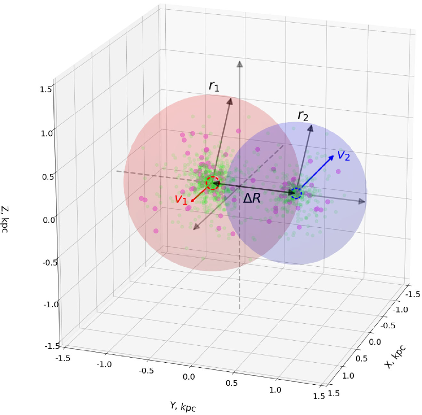
Figure 1: Sketch of principal system components and initial parameters. South and north BHs are represented by red and blue big dashed dots respectively and placed at initial separation $\Delta R$. BHs have initial velocities $V_{1}$ and $V_{2}$, for south and north nuclei respectively. Bulges with sizes $r_{1}$ and $r_{2}$ (each radius equals to 5 Plummer radiuses of according bulge) around nuclei consist of high mass particles and low mass particles, they are represented by purple and green dots respectively.

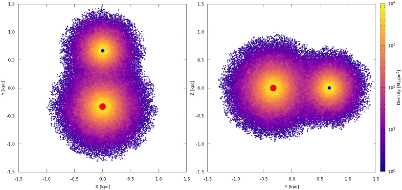
Figure 2: Initial density distributions at projection planes XY and YZ for physical model A. Red and blue dots are south and north BHs respectively.

Our N-body models consist of two bulges with embedded central BHs (Fig. 1). For creating the set of physical models we varied mass ratio between BHs and BH to bulge. Ratio between the total BHs mass and total bulges mass was chosen as $Q=m_{\bullet}/M_{\ast}=0.01$ (model A and C on Table 1) and 0.02 (model B and D on Table 1). Mass ratio for BHs and bulge is increased in comparison to predicted value (Kormendy & Ho (2013) and reference therein) due to active coalescence of galaxy. Interacting galaxy NGC 6240 most likely represents the major merging (Medling et al., 2011) and in this case we set mass ratios between the black holes $q=m_{\bullet 2}/m_{\bullet 1}=0.5$ (model A and B on Table 1) and $q=0.25$ (model C and D on Table 1). Mass of the primary (heavier) BH was obtained in range $8.7-20.8\times 10^{8}\rm M_{\odot}$ and for secondary (lighter) BH in range $2.6-8.7\times 10^{8}\rm M_{\odot}$. Primary and secondary BHs, which representing South and North nuclei, are considered special relativistic particles and located in bulges centres at separation $\Delta R$ on XY plane with initial velocities $V_{1,2}$. The initial orbital eccentricity of the two bulges in the simple point mass approximation was chosen as 0.5. BHs at this separation are not bound to each other.

Density distribution for each bulge is described by Plummer spheres (Plummer, 1911):

$$\rho_{1,2}(r)=\frac{3}{4\pi}\frac{M_{\ast 1,2}}{R_{1,2}^{3}}\Bigl{(}1+\Bigl{(}\frac{r}{R_{1,2}}\Bigr{)}^{2}\Bigr{)}^{-\frac{5}{2}},$$ (9)

where $M_{\ast 1,2}$ is the total stellar mass and $R_{1,2}$ is Plummer radius (Fig. 2). The same central density in each galaxy is provided by scaling the mass, size and number of particles consistently with BH mass ratio. Fixed Plummer radius for primary bulge $R_{1}=200$ pc gave us Plummer radius for secondary bulge $R_{2}=160$ pc for models A, B and $R_{2}=126$ pc for models C, D. After the generation of the particles distribution we simply add to the system the two central SMBH. Due to the very short dynamical merging scale (few Myr) of the two bulges, the initial Plummer distribution of the particles are quickly mixed up. Separation between the centres of bulges is 1 kpc according to the observable BH’s separation.

To mimic the presence of the molecular gas cloudy and clumpy mass structure in the bulges we introduce to our bulge particle system the multi mass prescription. Namely: ’high mass’ particles (HMPs), which represent perturbers and are associated with giant molecular clouds and/or stellar clusters, and ’low mass’ particles (LMPs), which represent field particles and are associated with individual stars. The main set of runs was done using total number of particles 500k (except model B1), where the number fraction of HMP is 10%. At each bulge the total HMP mass we set equal to the total LMP mass. For main set of runs (except models B4 and B1, see details below) we use HMP mass $\sim 1.3\times 10^{6}\rm M_{\odot}$ and LMP mass $\sim 1.4\times 10^{5}\rm M_{\odot}$.

Additionally for minimizing the effect of initial numerical parameters we have constructed numerical models based on physical model B (Table 1). We use larger number of particles $N=1000$k for model B1 (with HMP mass $\sim 6.5\times 10^{5}\rm M_{\odot}$ and LMP mass $\sim 7\times 10^{4}\rm M_{\odot}$), new randomization for initial particles coordinates and velocities for model B2, different starting point for $\mathcal{PN}$ terms turning on for model B3 (see Section 5), replacing HMP with LMP for model B4 with LMP mass $\sim 2.6\times 10^{5}\rm M_{\odot}$.

Table 1: Basic N-body models.

Physical models
Run	$q$	$Q$	$m_{\bullet 1}$	$m_{\bullet 2}$,	$M_{\ast 1}$,	$M_{\ast 2}$,
			$10^{8}\rm M_{\odot}$	$10^{8}\rm M_{\odot}$	$10^{10}\rm M_{\odot}$	$10^{10}\rm M_{\odot}$
A	0.5	0.01	8.67	4.33	8.67	4.33
B	0.5	0.02	17.34	8.66
C	0.25	0.01	10.4	2.6	10.4	2.6
D	0.25	0.02	20.8	5.2
Numerical models
Run	Characteristic property
B1	number of particles $N=1000$k
B2	randomisation seed
B3	starting point for $\mathcal{PN}$
B4	multi mass prescription

4 N-body code

For our simulations we used the publicity available $\varphi$-GPU code with the blocked hierarchical individual time step scheme and a $4^{th}$-order Hermite integration scheme of the equation of motions for all particles (Berczik et al., 2011). The individual timestep bin from the generalized “Aarseth” type criteria (Makino & Aarseth, 1992; Nitadori & Makino, 2008):

$$\Delta t_{i}=\eta_{p}\frac{A^{(1)}}{A^{(2)}}=\eta_{p}\sqrt{\frac{|\mathbf{a}||\mathbf{a}^{(2)}|+|\mathbf{\dot{a}}|^{2}}{|\mathbf{\dot{a}}||\mathbf{a}^{(3)}|+|\mathbf{a}^{(2)}|^{2}}}$$ (10)

where $\eta_{p}$ is parameter which controls the accuracy, $\mathbf{a}^{(k)}$ is the $k^{th}$ derivative of acceleration. In common block time step scheme the individual time steps $\Delta t_{i}$ are replaced by block time steps $\Delta t_{i,\rm b}=(1/2)^{n}$, where $n$ satisfies:

$$\Bigl{(}\frac{1}{2}\Bigr{)}^{n}\leq\Delta t_{i}<\Bigl{(}\frac{1}{2}\Bigr{)}^{n-1}$$

For minimization of the computational time the gravitational forces affecting the particle are divided into two types according to Ahmad-Cohen scheme. Regular forces apply from neighbour particles and irregular forces apply from more distinct particles, which have different time steps. It gives us the possibility to calculate irregular forces less often than regular forces.

In case of close encounters we should carefully integrate the orbit therefore we write the acceleration for $i$ particle from $j$ particle with mass $m_{j}$ placed on separation $r_{ij}$ in form:

$$\mathbf{a}_{i}=-\sum\limits_{j=1,\;j\neq i}^{N}\frac{Gm_{j}}{(r^{2}_{ij}+\varepsilon_{ij}^{2})^{3/2}}\mathbf{r_{ij}},$$ (11)

$$\varepsilon_{ij}^{2}=\alpha\frac{\varepsilon^{2}_{i}+\varepsilon^{2}_{j}}{2}$$ (12)

where $\varepsilon$ is individual softening parameter for each type of particles and $\alpha$ is reducing factor. In case of BH, HMP and LMP the softening parameters is $\varepsilon_{\rm BH}=0$, $\varepsilon_{\rm HMP}=10^{-4}$ and $\varepsilon_{\rm LMP}=10^{-5}$ respectively. When BHs interact with passing stars we reduce softening parameter using coefficient $\alpha=10^{-4}$ for more accurate calculation of acting forces. I.e. for these type of interaction we have the effective softening in a level of $7.1\times 10^{-7}$ or $7.1\times 10^{-8}$ respectively for the HMP and LMP. The individual softening in the code and also using the reducing factor for softening allow us more accurately taking in account the BH’s dynamical evolution even up to the $\mathcal{PN}$ merging phase.

The N-body simulations were run on five clusters: golowood at Kyiv (Ukraine), laohu at Beijing (China), kepler at Heidelberg (Germany), pizdaint at Zurich (Switzerland), juwels at Jülich (Germany).

5 Post-Newtonian BH and hardening

Table 2: Characteristic times for physical and numerical models

Run	$t_{\rm b}$	$t_{\rm h}$	$s_{\rm gw}=0.3\%s_{\rm nb}$				$s_{\rm gw}=3\%s_{\rm nb}$
			Subrun	$t_{\rm beg}$, NB	$t_{\rm beg}$, Myr	$t_{\rm merg}$, Myr	Subrun	$t_{\rm beg}$, NB	$t_{\rm beg}$, Myr	$t_{\rm merg}$, Myr
(1)	(2)	(3)	(4)	(5)	(6)	(7)	(8)	(9)	(10)	(11)
A	5.15	11.12	A.18	18	23.5	40.3	A.25	25	32.7	46.7
B	4.38	9.81	B.15	15	19.6	47.5	B.23	23	30.0	46.5
C	9.71	15.04	C.18	18	23.5	47.0	C.22	22	28.8	52.3
D	6.58	11.12	D.10	10	13.1	22.8	D.12	12	15.7	24.7
B1	4.15	9.81	B1.11	11	14.4	46.7	B1.16	16	20.1	39.3
B2	4.13	11.12	B2.11	11	14.4	44.7	B2.16	16	20.1	45.3
B3	4.30	11.12								51.3
B4	4.25	9.81								31.3

As mentioned above BHs are embedded as special massive relativistic particles located at the centres each bulges. The equation of motion was written via accelerations expressed through positions and velocities in $\mathcal{PN}$ formalism. $\mathcal{PN}$ theory is an approximate version of general relativity therefore in $\mathcal{PN}$ terms up to 3.5$\mathcal{PN}$ equation of motion schematically can be written in form

$$\mathbf{a}=\mathbf{a}_{\mathcal{PN}}+\frac{1}{c^{2}}\mathbf{a}_{1\mathcal{PN}}+\frac{1}{c^{4}}\mathbf{a}_{2\mathcal{PN}}+\frac{1}{c^{5}}\mathbf{a}_{2.5\mathcal{PN}}+\frac{1}{c^{6}}\mathbf{a}_{3\mathcal{PN}}+\frac{1}{c^{7}}\mathbf{a}_{3.5\mathcal{PN}}$$ (13)

where $a_{\mathcal{PN}}$ is the classical Newtonian acceleration, $a_{1\mathcal{PN},2\mathcal{PN},3\mathcal{PN}}$ correspond to energy conservation, $a_{2.5\mathcal{PN},3.5\mathcal{PN}}$ correspond to gravitational wave emission. Acceleration in the center-of-mass frame is

$$a=\frac{d\mathbf{V}}{dt}=-\frac{GM}{\Delta R^{2}}[(1+A)\mathbf{n}+B\mathbf{V}],$$ (14)

where $\mathbf{n}$ is normalized position vector, $\mathbf{V}$ is relative velocity (Blanchet, 2006). Coefficients A and B (see equations (182), (183), (185), (186) at Blanchet (2006) and references therein) are the complex functions of masses, velocities and separations.

Hard binary evolution can be split into two distinct regimes: classical and relativistic. Driven by the stellar-dynamical effects hardening in classical regime is constant during the long period:

$$s_{\rm nb}=\frac{d(1/a)}{dt}\approx\rm const.$$ (15)

At the next phase gravitational wave emission starts to be dominating dissipation force and hardening drastically decreases. After relativistic and classical hardenings are equal, in case of just 2.5$\mathcal{PN}$ corrections, average eccentricity and semimajor axis evolution is described as (Peters & Mathews, 1963; Peters, 1964a, b):

$$\Bigl{\langle}\frac{da}{dt}\Bigr{\rangle}_{\rm gw}=-\frac{64}{5}\frac{G^{3}m_{\bullet 1}m_{\bullet 2}(m_{\bullet 1}+m_{\bullet 2})}{a^{3}c^{5}(1-e^{2})^{7/2}}\Bigl{(}1+\frac{73}{24}e^{2}+\frac{37}{96}e^{4}\Bigr{)}$$ (16)

$$\Bigl{\langle}\frac{de}{dt}\Bigr{\rangle}_{\rm gw}=-\frac{304}{15}e\frac{G^{3}m_{\bullet 1}m_{\bullet 2}(m_{\bullet 1}+m_{\bullet 2})}{a^{4}c^{5}(1-e^{2})^{5/2}}\Bigl{(}1+\frac{121}{304}e^{2}\Bigr{)}$$ (17)

One can obtain the binary hardening during relativistic regime caused by gravitation wave emission (Khan et al., 2012)

$$s_{\rm gw}=\frac{64}{5}\frac{G^{3}m_{\bullet 1}m_{\bullet 2}(m_{\bullet 1}+m_{\bullet 2})}{a^{5}c^{5}(1-e^{2})^{7/2}}\Bigl{(}1+\frac{73}{24}e^{2}+\frac{37}{96}e^{4}\Bigr{)}$$ (18)

6 Results and discussion

The SMBHB evolution consists of three main time scales: period of time before gravitational bounding, the hardening time frame and a the time interval with strong GWs radiation emitting. The first two periods are described by the classical Newtonian dynamics. During the second phase we have a almost constant N-body hardening rate $s_{\rm nb}$ in short timescale. The last time interval is a relativistic mode with a combined classical and relativistic hardening rates $s_{\rm tot}=s_{\rm nb}+s_{\rm gw}$, where the latter term is dominating. Due to this we follows the next strategy.

As mentioned before, our SMBHB model at initial separation of 1 kpc is not a bound system. At first step we found the time of bounding our model binary system in a pure N-body runs and fitted the inverse semimajor axis $1/a$ with the linear function. The slope of this linear function is our constant N-body hardening. At the second step we obtain the theoretical relativistic hardening directly from (18). At the last third step we compare these hardening’s and choose the starting points to turn on the $\mathcal{PN}$ terms using two criteria $s_{\rm gw}=0.3\%s_{\rm nb}$ and $s_{\rm gw}=3\%s_{\rm nb}$. In totals for models A, B, C, D, B1, B2 we have one N-body run without $\mathcal{PN}$ terms (6 runs total) and two $\mathcal{PN}$ runs for each of Newtonian runs with different $\mathcal{PN}$ terms starting points $t_{\rm beg}$ (12 runs total) (Table 2). Relativistic sub-runs contain a number which presents a time when we turning on our $\mathcal{PN}$ terms. For models B3 and B4 we turn on $\mathcal{PN}$ terms directly from $t_{\rm beg}=0.0$. So, in total we have 20 individual runs.

Physical and numerical models in pure N-body regime (Fig. 3) show quick BHs bounding from beginning of simulations at time $t<10$ Myr (Table 2) with maximum value for model C. Binary starts to be hard at the time $t_{\rm h}<12$ Myr with longest time in model C due to the longest bound time. This time estimation has the error $\pm 0.66$ Myr because of time interval between the snapshots of the runs. Shrinking of the orbits in classical regime happens due to the interaction with surrounding stars. Semi-major axis is constantly decreasing as a linear function from gravitational bounding up to almost the merging time. With time the amount of particles which interact with binary drops, so called loss-cone depletion, and a hardening can gets more flat. For our simulations the $\mathcal{PN}$ relativistic terms start to working before this happens. So, in our cases the hardening does never stall. In all of our different physical models, as a primary BH mass increases, we see that the model inverse semimajor axis does not depend on the binary orbital parameters.

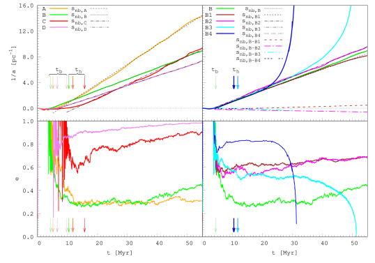
Figure 3: From top to bottom: evolution of inverse semimajor axis eccentricity in pure N-body regime for physical models A, B, C, D (left) and numerical models B1-4 (right) based on physical model B. Of note, for numerical models B3 and B4 we turned on $\mathcal{PN}$ terms from the start of simulations. For numerical models residuals between the model B and models B1-4 are shown as color dashed lines. Color arrows mark time when each system getting bound $t_{\rm b}$ (pale color) and hard $t_{\rm h}$ (intensive color). Colors chosen by main color scheme for each model.

The different numerical models show a good agreement of hardening rates. It shows independence of hardening rates from number of particles (in agreement with Berczik et al. (2006); Berentzen et al. (2009)), initial randomization (in agreement with Kompaniiets et al. 2021, in preparation), starting point of $\mathcal{PN}$ terms. For physical models C and D bounding pairs eccentricity (0.6-0.9) is higher than for the models A and B (0.3-0.4), but since in our N-body simulations the eccentricity is more or a less random, due to the stochastic nature of this process (Wang et al., 2014; Quinlan, 1996). For numerical models with non-physical differences we see eccentricity at a level of 0.6-0.8. Eccentricity slowly grows with time for both physical and numerical models (Preto et al., 2011).

Evolution with $\mathcal{PN}$ terms turned on shows a binary merging due to GW emission (Fig. 4, Fig. 5). We assume that the merging itself happens when the separation between the components is less than 4 Schwarzschild radius that equal 5.2 mpc for the models with $Q=0.01$ and 10.4 mpc for the models with $Q=0.02$. Model D with biggest mass of secondary BH has the shortest run and a model C with lowest mass of primary BH has the longest run. Inverse semimajor axis shows steady increase in classical regime and rapid rise at time when the GWs emission is dominant in dissipative force (Fig. 4, Fig. 5 left panels). Merging time for physical models is on ranges from 22 Myr to 53 Myr (Table 2, also see Sobolenko et al. (2016)). Eccentricity shows the same merging behavior in classical and relativistic regimes (Fig. 4, Fig. 5 right panels): after the binary is formed, eccentricity is almost constant in a classical regime and approaching to 0 (circular orbit) in a relativistic regime. Interestingly, the fastest-merging model D has the highest mass of primary BH and eccentricity around 0.9.

Compared to physical model B, models B1 with different number of particles and B2 with different initial randomization of particles positions and velocities do not show significant differences (also see Kompaniiets et al. 2021, in preparation). The choice of starting point $t_{\rm beg}$ does not affect merging time notably even for model B3 with $\mathcal{PN}$ terms turned on from the beginning. For models B1 and B2 the eccentricity is at the level of 0.6, for model B3 the eccentricity is a little bit less, at the level 0.5-0.6, for model B4 the eccentricity is higher and it is at the level 0.8. Model B4 with just a low mass particles merges even more quickly in time $\sim$30 Myr. Total differences in merging time for all of our numerical models is less then 10% (Table 2). Obtained merging time is larger than in research Kompaniiets et al. 2021, in preparation due to different initial physical parameters, such as total bulge mass and separation.

For each run the merging time for both physical and numerical models does not significantly change due to the variations of the $\mathcal{PN}$ terms starting points $t_{\rm beg}$. At the same time our technique of using two series (with 0.3% and 3% GW hardening compared to the N-body dynamical hardening) for hardening, gives us a quite good computational time savings (Table 3).

Table 3: Physical computational time at clusters.

Run	Node number	GPU card	Time
B3(NB+$\mathcal{PN}$)	16 nodes	Tesla K20	27.3 days
B(NB)+B.23($\mathcal{PN}$)	10 nodes	Tesla K20	2.6 days
		GeForce GTX 660

To check the accuracy of choosing the proper starting point we aligned the theoretical models hardening in relativistic regime (Fig. 6). The model’s relativistic hardening for physical runs of major merging A and B (with mean eccentricity at level of 0.3) shows a earlier decrease than the simple theoretical value. The merging time differences for model A is 25 Myr and for model B is around 20 Myr. For physical models C and D (with mean eccentricity is $>0.8$) the modeling relativistic hardening is at the same order as a theoretical value. For numerical models (with mean eccentricity $>0.5$) the difference between the theoretical model values is not so high and the best matching is observed in the models B3 and B4, where we turn on $\mathcal{PN}$ terms from the beginning. Numerical models B, B2, B3 have a same physical base, i.e. mass of BHs, similar N-body hardening but differs in binary eccentricity. According restricted number of our models, we did not find dependence of eccentricity and parameters of our systems. As expected from previous results the binary can form system with any initial eccentricity and statistically was found the trend to form more circular binary for steeper cusps (Khan et al., 2018). Also (Nasim et al., 2020) demonstrated the tendency of decreasing the eccentricity scattering with number of particles.

7 Conclusions

We have presented the direct N-body modeling with $\mathcal{PN}$ corrections up to 3.5$\mathcal{PN}$ for a central SMBHB in interacting galaxy NGC 6240. Creating the models set with a varying physical and numerical parameters gave us the limitations of major merging times for central binary. In a range of our parameters, we did not find any significant correlation between merging time and BHs mass or BH to bulge mass ratios. We understand that the set of initial physical conditions, generally speaking, can strongly effect of our merging time estimations. Also mass segregation can strongly affect a merging time (see Gualandris & Merritt (2012); Khan et al. (2018)), but to discuss this issue in context of our models with mixed mass prescription the further detail research is needed. Varying numerical parameters (randomization, number of particles, $\mathcal{PN}$ starting point) does not strongly affect of the merging time for BHs. The estimated time for a merging in NGC 6240 galaxy with the different physical parameters is less than $\sim$55 Myr. But this concrete number are valid only for our set of combination of initial mass ratios. In current case we limited our mass ratio ranges to the galaxy NGC 6240. Our numerical technique for turning on the relativistic $\mathcal{PN}$ forces not from the beginning of the run gave us the significant computational time savings. Further detailed research of rare dual/multiple BHs in dense stellar environment (based on observations data) can clarify the dynamical co-evolution of central BHs and their host-galaxies.

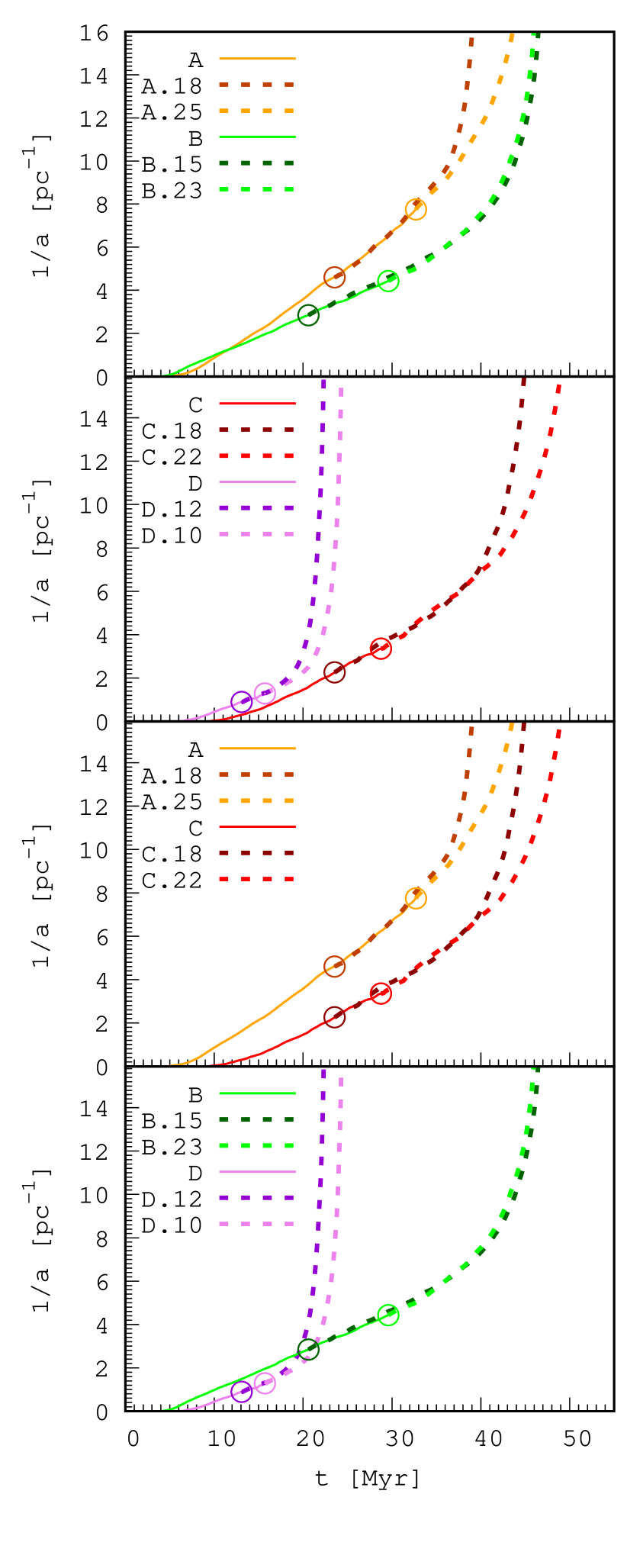
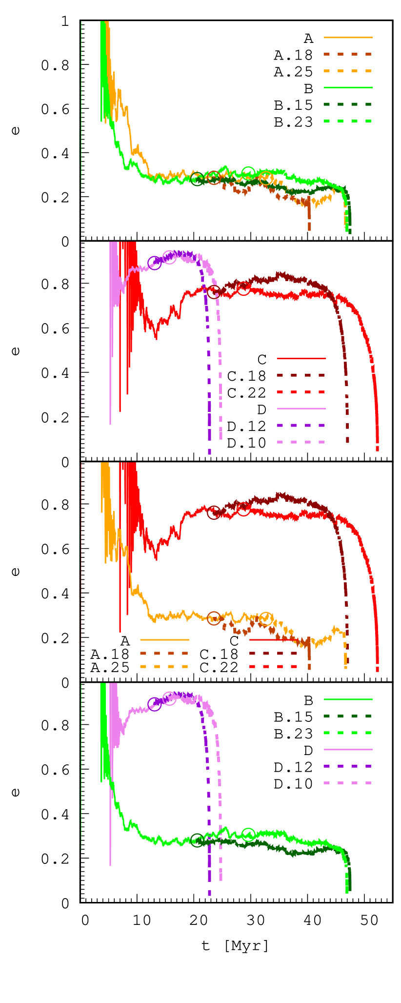
Figure 4: Inverse semimajor axis (left) and eccentricity (right) evolution for physical models A, B, C, D composed of N-body and $\mathcal{PN}$ runs. Start point for turning on $\mathcal{PN}$ terms from Table 2 noted by circles. Evolution for pure N-body regime are cut at time when latter $\mathcal{PN}$ runs start.

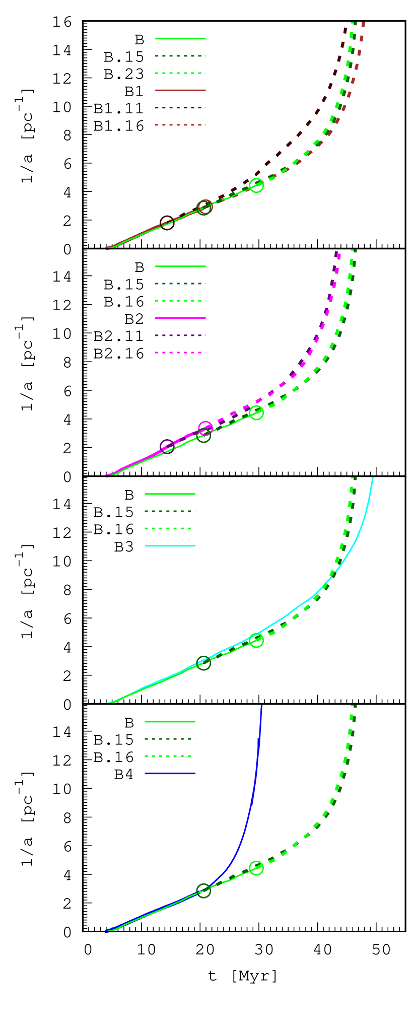
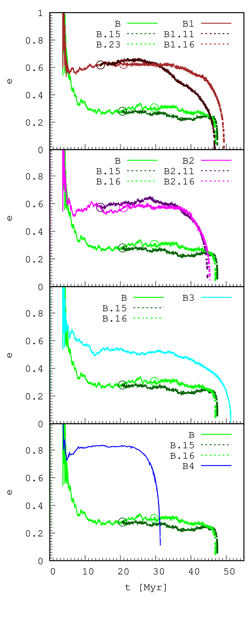
Figure 5: Inverse semimajor axis (left) and eccentricity (right) evolution for numerical models B1-4 composed of N-body and $\mathcal{PN}$ runs. Start point for turning on $\mathcal{PN}$ terms from Table 2 noted by circles. Evolution for pure N-body regime are cut at time when latter $\mathcal{PN}$ runs start.

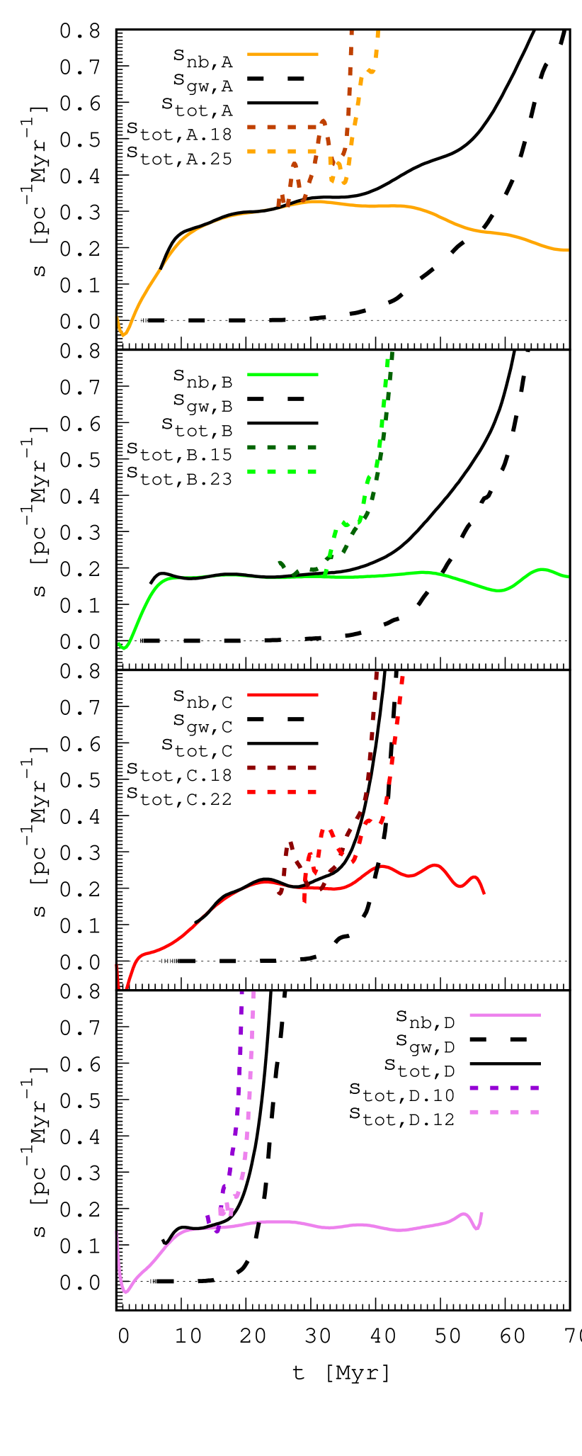
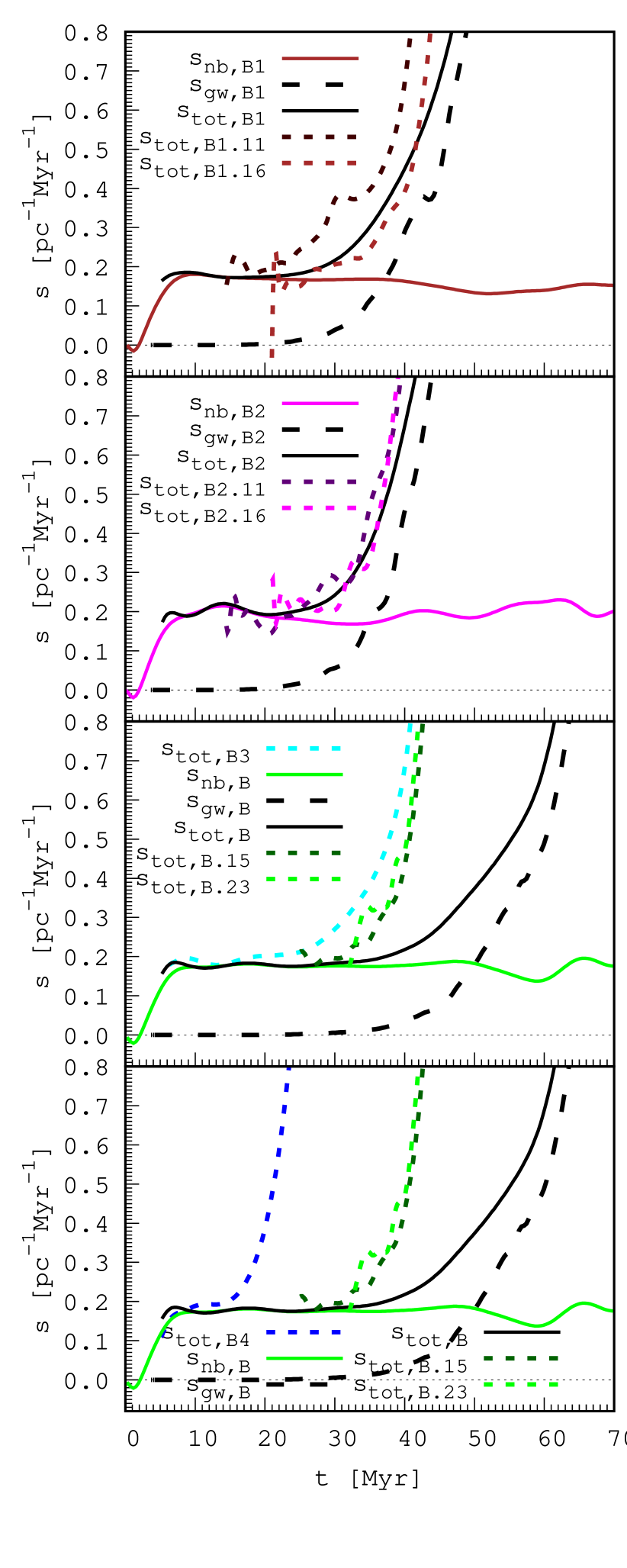
Figure 6: Hardening comparison for physical A, B, C, D (left) and numerical B1-4 (right) models from N-body simulations and theoretical relativistic hardening from (18)