Anisotropy in interface stress at the bcc-iron solid-melt interface: molecular dynamics and phase field crystal modelling

Abstract

The interface stresses at of the solid-melt interface are, in general, anisotropic. The anisotropy in the interfacial stress can be evaluated using molecular dynamics (MD) and phase field crystal (PFC) models. In this paper, we report our results on the evaluation of the anisotropy in interface stress in a bcc solid with its melt. Specifically, we study Fe using both MD and PFC models. We show that while both MD and PFC can be used for the evaluation, and the PFC and the amplitude equations based on PFC give quantitatively consistent results, the MD and PFC results are qualitatively the same but do not match quantitatively. We also find that even though the interfacial free energy is only weakly anisotropic in bcc-Fe, the interfacial stress anisotropy is strong. This strong anisotropy has implications for the equilibrium shapes, growth morphologies and other properties at nano-scale in these materials.

1 Introduction

The properties of the solid-melt interface in crystalline solids is of great fundamental interest and practical importance in many problems such as solidification and crystal growth [1]. Specifically, the interfacial energy plays a key role in nucleation [2, 3] and the interfacial energy anisotropy plays a key role in determining (a) the equilibrium shape of nanoparticles (see, for example, [4, 5]) and (b) the morphology of the growing crystals (see, for example, [6] for a review).

Several experimental methods (equilibrium shape, grain boundary grooving, nucleation, wetting and dendritic growth) have been used to measure the interfacial free energy and its anisotropy [7]. However, given the challenges associated with these experimental studies, theoretical and computational studies are also very common; see, for example, [7, 8, 9, 10]. Specifically, both molecular dynamics (MD) and phase field crystal (PFC) methods have been employed to successfully evaluate interfacial energies and their aniosotropy; see, for example, [10] for MD studies and [11, 12, 13] for PFC studies.

In a crystalline solid in contact with its melt, one can distinguish interface energy from interface stress; the energy associated with the formation of a new interface at constant stress is the interface energy while the energy associated with deforming the interface is the interface stress [14]. Further, the properties of a crystalline solid are necessarily anisotropic [1], and, hence, like the interfacial free energy and interface stress is also known to be anisotropic: see, for example [15, 16, 17]. The effect of such interface stress on solid-melt equilibrium is well known; see [14, 18, 19] for example.

Given the difficulties in the experimental determination of interface stress, simulations have been used in the past decade to determine interface stress. For example, Mishin and Frolov, in a series of papers, have used MD to determine interface stress in several fcc materials [20, 21, 22, 23]. Similarly, the PFC methodology has been used in to study the interface stress in 2-D hexagonal materials [24].

In this paper, we are interested in the evaluation of interfacial stresses and their anisotropy in bcc solids using both PFC and MD. Given that PFC can be considered as a time-averaged MD, we want to compare the interfacial stress evaluated using these two methods. Further, it is known that the interfacial free energy anisotropy is weak in bcc solids [11, 12, 25]; hence, we are interested in answering the question, namely, whether the interfacial stress anisotropy is also weak in such solids. Specifically, we evaluate interface stresses for the bcc iron in contact with its melt; the interface stress is evaluated using molecular dynamics (MD) simulations, the phase field crystal (PFC) method and the amplitude equations of the PFC method.

The rest of the paper is organised as follows: in Section 2, we describe the MD formulation and simulation methodologies. The formulation for evaluating interface stresses using MD is well known in the literature; so, we only give a brief description for the sake of completion. However, we describe the simulation methodology in detail. In Section 3, we describe the PFC formulation and the amplitude equations derived from PFC. Here again, the PFC formulation is well documented in the literature and hence we only describe it very briefly for the sake of completion. On the other hand, we extend the amplitude equation formulation previously for 2D hexagonal lattices [24] to bcc solids; hence, we describe this formulation in greater detail below. In Section 4, we present the results from our MD and PFC simulations on the interfacial stress and its anisotropy in bcc iron in contact with its melt and compare the results from MD with those obtained from PFC and amplitude expansion. While the PFC and amplitude expansion results agree quantitatively, the agreement between MD and the PFC/Amplitude equations is qualitative. Finally, we conclude the paper with a brief summary of salient results from this work.

2 MD: Formulation and simulation methodology

Consider the solid-melt interface in a single component system as shown in Fig 1.

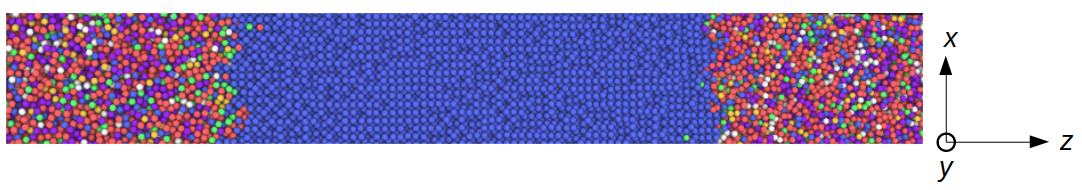
Figure 1: A simulation block of solid iron (bcc – in blue at the middle of the simulation cell) in contact with iron melt (on the left and right ends of the simulation cell). The interface normal is along the z-direction of the simulation cell (which is aligned with the (001) of the crystallographic direction in this particular case.

Our aim is to evaluate the interface stress at this solid-melt interface; specifically, the interface consists of solid (bcc) iron and its melt. In order to evaluate the interface stress, the solid is non-hydrostatically stressed. The application of non-hydrostatic stress is known to change the temperature and pressure of the system. In this paper, we report the interface stresses obtained under isothermal conditions; that is, the solid and the melt are maintained at the same temperature both before and after the application of the non-hydrostatic stress to the solid. There are other paths, such as the iso-fluid path for example, in which both the pressure and temperature are maintained to be the same both before and after the application of the non-hydrostatic stress to the solid. However, here, we restrict ourselves to the studies carried out using iso-thermal paths. We are also interested in the anisotropy in the interface stress. Hence, we set up simulations with different normals for the solid surfaces that are in contact with the melt.

2.1 Formulation

The formulation and methodology used to evaluate surface stress using MD is given in detail in the papers of Frolov and Mishin [21, 23]. For the sake of completeness in this section we describe the salient aspects of the formulation relevant for our work.

Let the square braces $[(\cdot)]$ represent the interface excess quantity in the property $(\cdot)$; then, the interface excess in the property Z can be represented as a ratio of two determinants [23] as follows:

$$[Z]_{XY}=\frac{\begin{vmatrix}[Z]&[X]&[Y]\\ Z^{s}&X^{s}&Y^{s}\\ Z^{m}&X^{m}&Y^{m}\\ \end{vmatrix}}{\begin{vmatrix}X^{s}&Y^{s}\\ X^{m}&Y^{m}\\ \end{vmatrix}}$$ (1)

where, X and Y are any two extensive properties chosen from energy (U), entropy (S), volume (V) and number of atoms (N); the quantities in the first row of the determinant in the numerator are for the chosen layer of the interface; for the quantities in the other rows of the determinant in the numerator and the determinant in the denominator, the superscripts $s$ and $m$ represent the homogeneous regions of solid and melt phases, respectively.

For the isothermal path simulations, using the Eq. 1, the excess interface stress $[\tau_{ij}]$ while keeping the volume and number of atoms a constant (that is, choosing $N$ for $X$ and $V$ for $Y$ in the expression) is as follows:

$$[\tau_{ij}]_{NV}=\frac{\begin{vmatrix}[(\sigma_{ij}+\delta_{ij}P)V]&[N]&[V]\\ (\sigma_{ij}^{s}+\delta_{ij}P)V^{s}&N^{s}&V^{s}\\ 0&N^{m}&V^{m}\\ \end{vmatrix}}{\begin{vmatrix}N^{s}&V^{s}\\ N^{m}&V^{m}\\ \end{vmatrix}}$$ (2)

where $\delta_{ij}$ is the Kronecker delta (that is, $\delta_{ij}$ is unity when $i=j$ and zero otherwise), $\sigma_{ij}$ is the stress and $P$ is the pressure. Expanding the determinants and simplifying, we obtain

$$[\tau_{ij}]_{NV}=\frac{1}{A}\left\{[(\sigma_{ij}+\delta_{ij}P)V]-(\sigma_{ij}^{s}+\delta_{ij}P)V^{s}\left[\frac{[N]V^{m}-N^{m}[V]}{N^{s}V^{m}-N^{m}V^{s}}\right]\right\}$$ (3)

Given Eq. 3, we can obtain the excess interface stress by carrying out an isothermal simulation in which the volume ($V$) and the number of atoms $N$ are maintained a constant; that is , by carrying out a simulation in the $NVT$ ensemble. In order to carry out the simulation at constant temperature, first we need to evaluate the equilibrium coexistence temperature between the solid and melt – across different planar interfaces. Note that in the case of stressed solid, the equilibrium temperature can change; however, since we are using the isothermal path, the temperature is maintained a constant in our simulations. In addition, in order to stress the solid non-hydrostatically, we use the stress-control-via-strain-control approach. The simulation methodology consists of the following steps. First, we evaluate the equilibrium temperature of coexistence for the two phases across a planar interface. Second, we determine the elastic constants of the solid phase; the elastic moduli thus obtained serve as a benchmark for the potential used, to validate the phase co-existence (using the virial stress and the compliance tensor), and, to relate the imposed strains to applied stresses in the solid. Third, we set up a simulation box in which the solid and the melt are in co-existence and the solid is stressed by imposing a given strain. After equilibration, we evaluate the relevant quantities of interest, namely, interface stresses (using virial stress).

2.2 Simulation Details

Our MD simulations are performed using Large-scale Atomic/Molecular Massively Parallel Simulator (LAMMPS). One of the crucial inputs to the MD simulation is the potential. In this study, we have used the EAM potential developed by Mendelev et al. [26]; Mendelev et al. developed this potential to be appropriate for both the solid and liquid phases of iron; both first principles and experimental data was used in the fitting exercise.

A simulation block of solid-melt system with periodic boundary conditions in all three directions is used; in order to align the interface normal to be along the (001), (110) and the (111) planes of the b.c.c solid, the following three geometries are used:

• the (100), (010) and (001) directions of the crystal along the x- y- and z-directions of the simulation box, respectively;

• the (001), (1$\bar{1}$0) and (110) directions of the crystal along the x-, y- and z-directions of the simulation box, respectively; and,

• (1$\bar{1}$0), (11$\bar{2}$) and (111) directions of the crystal along the x-, y- and z-directions of the simulation box, respectively.

For example, in Fig. 1, we show the simulation block with the interface aligned along the (001) direction.

In the following sections, we describe the calculation of melting point for these different geometries (using the solid-melt coexistence method) and the evaluation of elastic moduli of the solid at the melting point (using the direct method).

2.2.1 Evaluation of equilibrium melting temperature

The determination of melting temperature is essential for setting up the coexistence of solid-liquid system in the simulations. The melting temperature is determined in two steps. In the first step, we obtain an approximate melting temperature of the system by carrying out bulk heating of a solid b.c.c iron block (of 72000 atoms with periodic boundary conditions in all three directions) and identifying the temperature at which abrupt change in potential energy is observed as the tentative melting point. In order to refine the melting temperature thus calculated, we use the coexistence method proposed by Morris et al. which is widely used in the literature: see for example [27, 28, 29].

In the co-existence method, a simulation block consisting of solid and liquid phases is equilibrated at temperatures above and below the estimated melting temperature using the isobaric and isothermal ensemble (NPT) and the potential energy curves are observed during equilibration at these different temperatures. For example, for the geometry of (100), (010) and (001) crystallographic directions oriented along the x- y- and z-directions, the potential energy curves for different temperatures are as shown in Figure 2. The potential energy curve for systems equilibrated below 1820 K decreases, indicating that the system is freezing, while, those equilibrated above 1820 K increase, indicating that the system is melting. At 1820 K, potential energy is a constant indicating the solid-melt coexistence. By plotting the slope of the linear regions of potential energy change (obtained using linear fit) as a function of temperature (see the second plot in Fig. 2), we identify the point where slope of potential energy is zero as the equilibrium melting temperature. Similarly, for other geometries also the melting temperature is calculated and the results are tabulated in Table. 1. The error bars are obtained by averaging over three simulations.

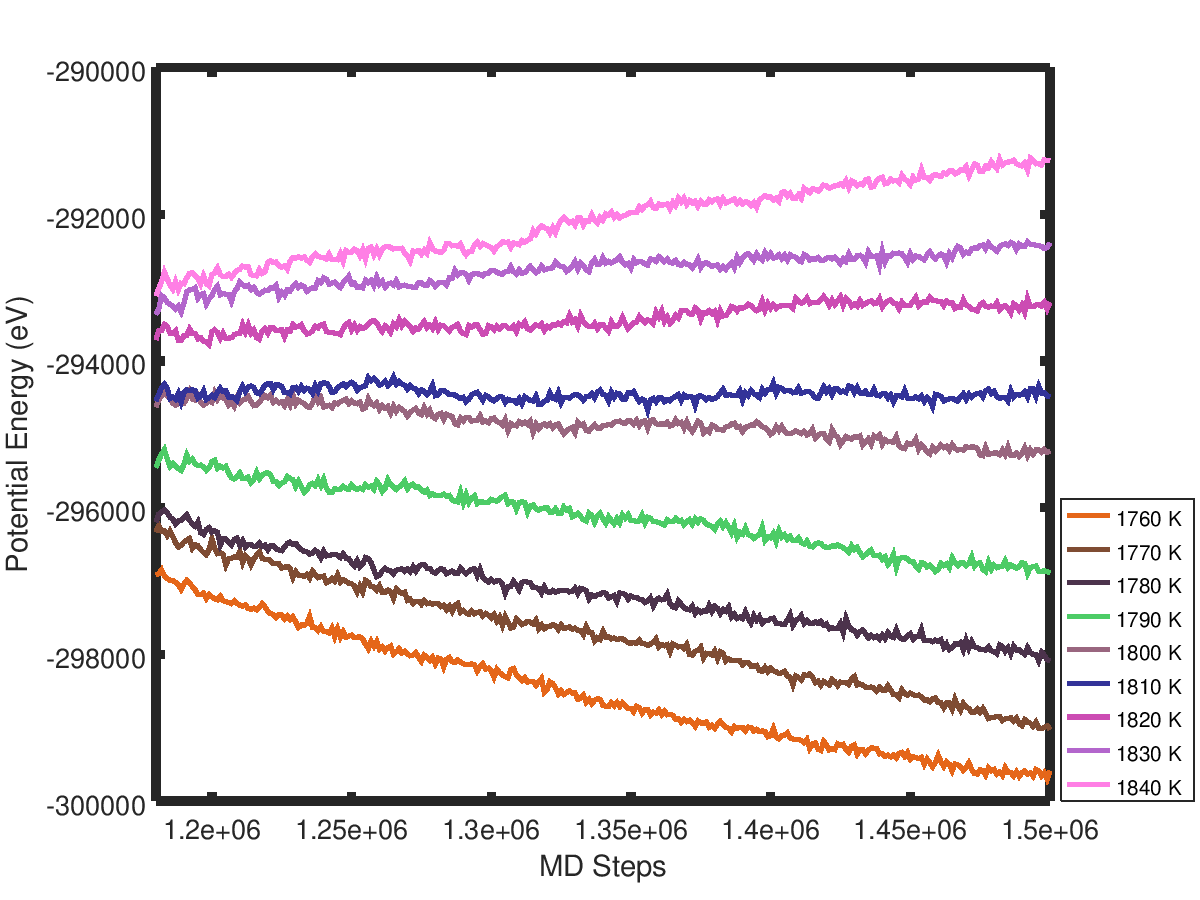
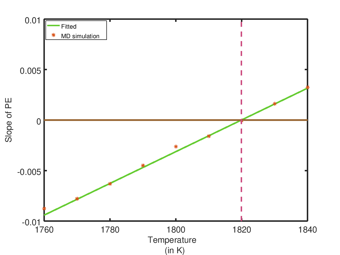
Figure 2: Left figure: Potential energy as a function of time at different temperatures obtained using NPT ensemble simulations, and, Right figure: the slope of the linear portions of the potential energy versus time plots as a function of temperature. The melting point (dotted vertical line) is the point at which the slope of the potential energy versus time plot is zero.

Interface plane	X	Y	Z	Equilibrium melting temperature
orientation				K
(001)	[100]	[010]	[001]	1820 $\pm$ 1
(110)	[001]	[1$\overline{1}$0]	[110]	1817 $\pm$ 3
(111)	[1$\overline{1}$0]	[11$\overline{2}$]	[111]	1820 $\pm$ 2

Table 1: Equilibrium melting temperature for different geometries across a planar solid-melt interface obtained using the coexistence method.

2.2.2 Calculation of elastic constants

The elastic constant is computed using the direct method and simulations in an NVT ensemble – as described in the LAMMPS manual [30]. We use a strain of 0.2% . The elastic constants at 0 K, room temperature (300 K) and at the melting temperature ($T_{m}=1820$ K) obtained using our computations are given in Table 2. These compare well with the constants reported for 0 K using first principle calculations (as reported by Mendelev et al. [26], the experimentally reported constants at 300 K [31] and the near melting point constants reported [32] (albeit using a different potential and different method of evaluation).

	Elastic constants	$C_{11}$	$C_{12}$	$C_{44}$
		(GPa)	(GPa)	(GPa)
Current	0 K	243	131	115
study	300 K	$230\pm 2$	$134\pm 2$	$105\pm 5$
	1820 K	132	103	73
Reported	0 K (DFT)	243.7	145.1	115.9
Values	300 K (Expt)	234	131	115
	1812 K (MEAM potential / MD simulations)	141	129.2	68.1

Table 2: Elastic constants of Fe from the current simulations compared with reported values in the literature.

2.2.3 Interface stresses in solid-melt interface at constant temperature

Once the solid-melt coexistence is achieved, the simulation block is subjected to biaxial deformation by applying equal magnitude of stress in x and y directions to generate non-hydrostatic stresses in the solid by scaling the dimensions of the simulation block. The simulation block is subjected to both tension and compression biaxially. The deformation destroys the phase equilibrium and hence the coexisting phases are again re-equilibrated in the canonical ensemble (NVT) for 2 million time steps after deformation; this is followed by production run of 4 million time steps and the results of the simulation are saved after every 10000 time steps. In our simulations each time step corresponds to 1 femtosecond. The interface stresses are obtained using Eq. (3) by analysing the saved results and generating the required quantities (such as volume, atomic stress etc) from the simulation results.

2.2.4 Validation of phase coexistence

When the solid is deformed non-hydrostatically, the pressure in the melt changes and the change in the pressure is given by the following analytical expression:

$$P-P_{H}=\frac{V^{s}}{2(V^{m}-V^{s})}[S_{1111}q_{11}^{2}+2S_{1122}q_{11}q_{22}+S_{2222}q_{22}^{2}]$$ (4)

where $P_{H}$ is hydrostatic pressure in the absence of any applied stress, $S_{ijkl}$ is the compliance tensor, $V^{s}$ and $V^{m}$ are the volumes of the homogeneous solid and melt respectively, and $q_{ij}$ are the components of the virial stress (that is, $\sigma_{ij}+p\delta_{ij}$) – see Eq. 37 of  [22] (Note that Frolov and Mishin’s version also contains a $T_{H}$ term in the numerator on the RHS which, we believe, is a typographical error). In Fig. 3, we compare our numerical results for the $P-P_{H}$ obtained using MD simulations with that given by the analytical expression above and the two match very well indicating that our simulations are in agreement with the analytical prediction. Note that the given figure is for one of the geometries, namely, x-, y- and z-directions of the simulation cell are aligned with the (100), (010), and (001) crystallographic directions respectively; we find similar agreement for the other two geometries also.

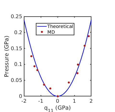
Figure 3: Equilibrium pressure of the liquid as a function of the non-hydrostatic stress component in the solid (which is subjected to biaxial stress).

2.2.5 Identification of the interface position

In order to calculate the interface stress components, we need to evaluate the extensive quantities for homogeneous bulk solid and melt regions as well as the interface region. Hence, we need to evaluate the position of the interface and its width; the homogeneous bulk solid and melt regions are identified with respect to the instantaneous position of the interface. Hence, the determination of the position of the interface and its width are crucial.

Due to thermal fluctuations, the position of the interface keeps changing with time during the MD run. In order to locate the instantaneous interface position, a structural order parameter ($\phi_{k}$), is calculated using the given equation:

$$\phi_{k}=\frac{1}{14}\sum_{i}|r_{i}-r_{bcc}|^{2}$$ (5)

where r_i denotes the distances of the first and second nearest neighbours in the simulated structure and r_bcc refers to the first and second nearest neighbour distance for the ideal bcc crystal. This definition of order parameter is known to result in $\phi_{k}\approx 0$ for an atom in the bcc solid and non-zero for atoms in the melt regions: see for example [29, 9]. Thus, the $\phi_{k}$, defined for every atom $k$ helps us distinguish the solid and liquid regions.

The order parameter $(\phi_{k})$ is further smoothed using the following equation to remove the fluctuation in a calculated values:

$$\phi(z_{p})=\frac{\sum_{k}w(z_{p}-z_{k})\phi_{k}}{\sum_{k}w(z_{p}-z_{k})}$$ (6)

where weighting function $w$ is defined as $w(z_{p})=\left[1-(\frac{z_{p}}{d})^{2}\right]^{2}$ for $|z_{p}|<d$ (cut-off distance), else $w(z_{p})=0$ and $z_{k}$ is atom coordinates of atom $k$. In the z-direction the simulation block is discretised into bins and order parameters are averaged over all atoms in the bin; we use a cut-off distance of $7\AA$ in order to avoid the smearing out of the information [33]. The position of the interface at any instant is determined by fitting a function $f(z)=c_{1}+c_{2}\tanh\left(\frac{z-c_{3}}{c_{4}}\right)$ to the order parameter data ($\phi(z_{p})$), where z is the coordinates of the atoms along the direction perpendicular to the solid-melt interface and the fitting parameter c₃ denotes the interface position [29]. The plot of the order parameters along with the fit of the hyperbolic tangent function is shown in Figure 4.

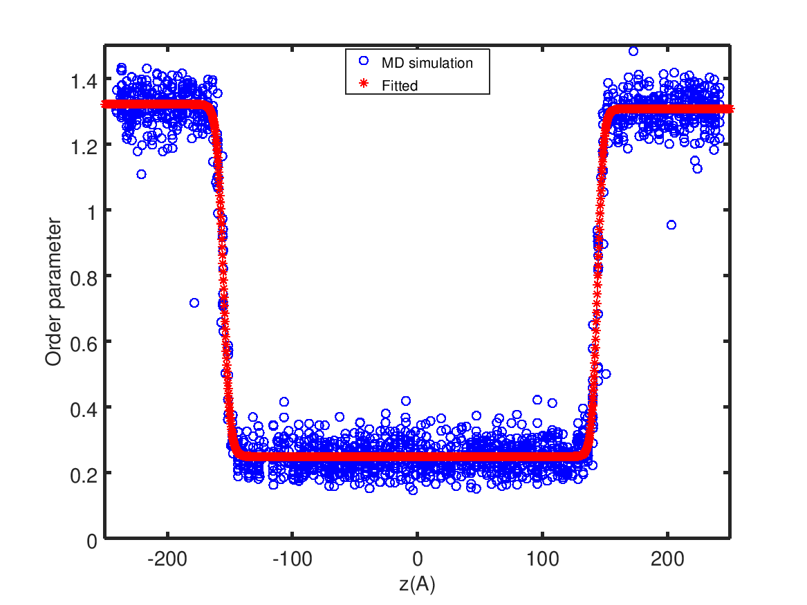
Figure 4: Calculated order parameters to determine interface position with respect to a coordinate perpendicular to the solid-melt interface.

In order to make sure that the integration for the interface properties is done over the entire interface, we have to choose an interface width (‘d’) which extends from bulk melt to bulk solid or vice versa. In this study, we have used a $d$ of 20$\AA$.

3 Phase field crystal model: Formulation and simulation methodology

The PFC model has been widely used to investigate elastic and plastic processes in materials as well as solid-solid and solid-liquid interfacial properties [34, 35, 36, 37, 38, 39, 40, 41, 42, 43, 44]. It has its roots in the density functional theory of freezing as discussed in detail in Ref. [45]. Variants of the PFC model have been proposed to generalise the model to describe various crystal symmetries [46, 47, 48]. Here, we restrict our attention to the simplest formulation of PFC since we focus on the relation of the surface stress and the underlying crystal symmetry, although the following derivation could be easily generalised for other PFC models. Recently, Liu and Wu have investigated the surface stresses of the 2D hexagonal lattice [24]. Based on the formalism and calculation in their work, we investigate the interfacial stress for bcc-liquid interface.

3.0.1 Free energy functional

In Ref. [34, 35], the dimensionless form of the simplest PFC free energy functional is

$$F=\int d\vec{r}~{}\left\{\frac{\psi}{2}\left[-\epsilon+(1+\nabla^{2})^{2}\right]\psi+\frac{\psi^{4}}{4}\right\}$$ (7)

in which $\psi$ serves as the dimensionless density field relative to a reference state, and $\epsilon$ is a control parameter that determines the interfacial properties and elasticity of materials which can be set once the liquid structure factor of the material at the melting point is known [11, 35]. The chemical potential $\mu$ is defined as the functional derivative of $F$, namely

$$\mu=\frac{\delta F}{\delta\psi}=\left[-\epsilon+(1+\nabla^{2})^{2}\right]\psi+\psi^{3}.$$ (8)

The dynamics of the system simply follows the following conserved relaxation rule, ${\partial\psi/\partial t}=\nabla\cdot\nabla\mu$. According to thermodynamics, the chemical potential $\mu$ must be a uniform constant over the system at equilibrium.

3.0.2 Solid-liquid coexistence

PFC model would naturally form the liquid and solid coexistence by setting appropriate value of parameter $\epsilon$ and the mean density $\bar{\psi}$ [11]. The liquid phase is a homogeneous state, $\psi(\vec{r})=\bar{\psi}_{l}$. The corresponding free energy density is obtained straightforwardly from Eq. (7),

$$f_{l}=(-\epsilon+1)\frac{\bar{\psi}_{l}^{2}}{2}+\frac{\bar{\psi}_{l}^{4}}{4}.$$ (9)

In comparison, the solid phase could be expressed approximately by a mean density $\bar{\psi}_{s}$ and a group of density waves that reflects the symmetry of the solid,

$$\psi_{s}(\vec{r})\approx\bar{\psi}_{s}+\sum_{j}A_{j}e^{i\vec{K}_{j}\cdot\vec{r}}+\sum_{j}A_{j}^{*}e^{-i\vec{K}_{j}\cdot\vec{r}},$$ (10)

where $A_{j}$ and $A_{j}^{*}$ are the amplitude and its complex conjugate, respectively, of each density wave, and $\vec{K}_{j}$ is the reciprocal lattice vector (RLV). Based on the one-mode approximation, the solid state at coexistence can be well represented by employing only the set of principal RLVs. The reciprocal lattice to a bcc structure is a fcc structure. Therefore, the principal RLVs for a bcc structure is a group of 12 vectors, namely,

$$\vec{K}_{1} =\frac{K_{0}}{\sqrt{2}}\left(\hat{x}+\hat{y}\right),\qquad\vec{K}_{2}=\frac{K_{0}}{\sqrt{2}}\left(\hat{x}-\hat{y}\right),\qquad\vec{K}_{3}=\frac{K_{0}}{\sqrt{2}}\left(\hat{y}+\hat{z}\right),$$ (11)

$$\vec{K}_{4} =\frac{K_{0}}{\sqrt{2}}\left(\hat{y}-\hat{z}\right),\qquad\vec{K}_{5}=\frac{K_{0}}{\sqrt{2}}\left(\hat{x}+\hat{z}\right),\qquad\vec{K}_{6}=\frac{K_{0}}{\sqrt{2}}\left(\hat{x}-\hat{z}\right),$$ (12)

and their counterparts $\vec{K}_{\bar{j}}=-\vec{K}_{j}$. Since the crystal symmetry of the bcc lattice ensures that the all density waves have the same amplitude $A_{s}$, the free energy density of the solid is readily derived from Eq. (7),

$$f_{s} =(-\epsilon+1)\frac{\bar{\psi}_{s}^{2}}{2}+\frac{\bar{\psi}_{s}^{4}}{4}+6[-\epsilon+(1-K_{0}^{2})^{2}]A_{s}^{2}+18\bar{\psi}_{s}^{2}A_{s}^{2}+48\bar{\psi}_{s}A_{s}^{3}+135A_{s}^{4},$$ (13)

where $K_{0}=1$ so that free energy is minimised with respect to $K_{0}$. By minimising the free energy density with respect to $A_{s}$, we obtain the amplitude of density waves of the solid phase,

$$A_{s}=-\frac{2}{15}\bar{\psi}_{s}+\frac{1}{15}\sqrt{5\epsilon-11\bar{\psi}_{s}^{2}}$$ (14)

which is coupled to $\epsilon$ and $\bar{\psi}_{s}$.

The coexistence densities for solid-liquid systems with planar interfaces are determined by requiring both phases have the same chemical potential and pressure. Detailed calculations are discussed in Ref. [11]. For small values of $\epsilon$, the coexistence densities can be expressed as a series expansion of $\epsilon^{1/2}$,

$$\bar{\psi}_{s} \approx\epsilon^{1/2}\psi_{s0}+\epsilon^{1}\psi_{s1}+\epsilon^{3/2}\psi_{s2}+\mathcal{O}(\epsilon^{2})$$ (15)

$$\bar{\psi}_{l} \approx\epsilon^{1/2}\psi_{l0}+\epsilon^{1}\psi_{l1}+\epsilon^{3/2}\psi_{l2}+\mathcal{O}(\epsilon^{2}).$$ (16)

For bcc lattices, the coefficients are computed using the common tangent construction which leads to $\psi_{s0}=\psi_{l0}=\psi_{c}\equiv-\sqrt{45/103}$ and $\psi_{s1}=\psi_{l1}=0$. Notably, the miscibility gap $\bar{\psi}_{s}-\bar{\psi}_{l}$ is proportional to $\epsilon^{3/2}$.

3.0.3 Interfacial energy

The interfacial energy is the excess free energy of forming an interface [20], and in the PFC model the interfacial energy of a planer interface can be evalutated by the following expression shown in Ref. [11],

$$\gamma=\Sigma^{-1}\int d\vec{r}\left[f-\left(\frac{\psi-\bar{\psi}_{l}}{\bar{\psi}_{s}-\bar{\psi}_{l}}f_{s}+\frac{\psi-\bar{\psi}_{s}}{\bar{\psi}_{l}-\bar{\psi}_{s}}f_{l}\right)\right],$$ (17)

where $\Sigma$ is the area of the planar interface and $f$ represents the free energy density, which is the integrand in Eq. (7).

3.1 Amplitude Equations for PFC model

In addition to the PFC model, the amplitude equations (AEs) are often employed to show how the density waves break its symmetry at the interface which eventually leads to anisotropic properties of the interface. The amplitude equations are obtained using the multi-scale expansion of the PFC model, assuming that the amplitude profile varies much more slowly than the underlying periodicity of the crystal. As shown in Ref. [11], the amplitude of density waves depends on a slow spatial variable $\vec{R}=\epsilon^{1/2}\vec{r}$, and thus, we can express the density field as

$$\psi(\vec{R},\vec{r})\approx\epsilon^{1/2}\left[\psi_{c}+\epsilon n(\vec{R})+\sum_{j=1}^{6}A_{j}(\vec{R})e^{i\vec{K}_{j}\cdot\vec{r}}+\sum_{j=1}^{6}A_{j}^{*}(\vec{R})e^{-i\vec{K}_{j}\cdot\vec{r}}\right],$$ (18)

where $n(\vec{R})$ is the average density over a unit cell. As a consequence, the effective free energy functional with respect to amplitudes and average density becomes

$$F \cong\epsilon\int d\vec{R}~{}\sum_{j=1}^{6}|\hat{L}_{j}A_{j}|^{2}+\bar{f}_{local}+\mathcal{O}(\epsilon^{2}),$$ (19)

$$\hat{L}_{j} \equiv 2i\vec{K}_{j}\cdot\nabla_{R}+\epsilon^{1/2}\nabla_{R}^{2},$$ (20)

$$\bar{f}_{local} \equiv(-1+\epsilon^{-1})\frac{\psi_{c}^{2}}{2}+\psi_{c}(-\epsilon+1)n+\epsilon\frac{n^{2}}{2}+\frac{\psi_{c}^{4}}{4}+\epsilon\psi_{c}^{3}n$$

$$+(3\psi_{c}^{2}+6\epsilon\psi_{c}n-1)\sum_{j=1}^{3}|A_{j}|^{2}+6(\psi_{c}+\epsilon n)(A_{1}A_{2}A_{3}+A_{1}^{*}A_{2}^{*}A_{3}^{*})$$

$$+\frac{3}{2}\sum_{j=1}^{3}|A_{j}|^{4}+6\sum_{j=1}^{3}\sum_{k>j}^{3}|A_{j}|^{2}|A_{k}|^{2},$$ (21)

in which $\nabla_{R}$ denotes the gradient with respect to $\vec{R}$. The second term in Eq. (19) is a non-linear function of free energy density which simply depends on local density and amplitudes. Furthermore, the amplitudes $A_{j}$ and average density $n$ follow the non-conserved and conserved relaxational dynamics, respectively,

$$\frac{\partial A_{j}}{\partial t} = -\frac{\delta F}{\delta A_{j}^{*}}=-\hat{L}_{j}^{2}A_{j}-\frac{\partial\bar{f}_{local}}{\partial A_{j}^{*}}$$ (22)

$$\frac{\partial n}{\partial t} = \nabla^{2}\frac{\delta F}{\delta n}=\epsilon\nabla_{R}^{2}\frac{\partial\bar{f}_{local}}{\partial n}.$$ (23)

Due to the dependence of $\hat{L}_{j}$ on $\vec{K}\cdot\nabla_{R}$, the profile of amplitudes would vary differently across the interface depending on surface orientation which leads to anisotropic interfacial properties, as shown by Wu and Karma [11].

In bulk phases, $n$ and $A_{j}$ are uniform and the free energy densities, $\bar{f_{s}}$ and $\bar{f}_{l}$, of solid and liquid, respectively, are expressed by $\bar{f}_{local}(n,A_{j})$ with different average density and amplitudes,

$$\bar{f}_{s}=\bar{f}_{local}(n_{s},\bar{A}),\qquad\bar{f}_{l}=\bar{f}_{local}(n_{l},0)$$ (24)

where $n_{s}$ and $n_{l}$ are the average density of solid and liquid, respectively, and $\bar{A}$ is the common amplitude among the density waves, which corresponds to $A_{s}$ in PFC, $A_{s}\cong\epsilon^{1/2}\bar{A}$. Similar to the case of the original PFC model, the values of $n_{s}$, $n_{l}$ and $\bar{A}$ at solid-liquid coexistence are solved by common tangent construction to $n_{s}$ and $n_{l}$ and free energy minimisation with respect to $\bar{A}$.

3.1.1 Deformation

Before deriving interfacial stress for the PFC model, it is necessary to identify the measure of the deformation such as displacement vector $\vec{u}$ in the PFC model, which has been discussed in Refs. [49, 50, 36, 37]. The deformation could be regarded as a transformation of lattice basis defined as

$$e^{i\vec{K}\cdot\vec{r}}\rightarrow e^{i\vec{K}\cdot\vec{r}\,^{\prime}}=e^{i\vec{K}\cdot(\vec{r}-\vec{u})}$$ (25)

which corresponds to shifting a lattice point $\vec{r}\,^{\prime}$ to a new position $\vec{r}$ with a displacement $\vec{u}$. Then, the phase of $A_{j}$’s is associated with the local displacement field $\vec{u}$. This description works well within bulk solid, where the crystal symmetry is preserved; however, it is not sufficient for the interface region where atoms subjected to asymmetric interatomic potential. Therefore, an additional phase, $\varphi$, in the amplitudes is required to completely capture lattice deformations due to asymmetric forces experienced by atoms at the interface. The general form of the amplitude can be expressed as

$$A_{j}=a_{j}e^{-i\vec{K}_{j}\cdot\vec{u}}e^{i\varphi}$$ (26)

where $a_{j}\equiv|A_{j}|$ is the magnitude of amplitudes and $\varphi$ is the mean phase of the three amplitudes, $A_{1}A_{2}A_{3}=|A_{1}A_{2}A_{3}|e^{3i\varphi}$, which is an additional degree of freedom apart from the displacement vector. For a stress-free solid-liquid system at equilibrium, $\vec{u}$ is homogeneous and $\varphi$ vanishes in bulk solid but both of them vary across the interface and their variations are in the order of $\epsilon$, $\nabla\vec{u}\sim\nabla\varphi\sim\epsilon$.

With Eq. (26), one can readily quantify the excess free energy contribution due to strains by applying $\hat{L}_{j}$ to the amplitudes,

$$\hat{L}_{j}A_{j}=\hat{L}_{j}a_{j}e^{-i\vec{K}_{j}\cdot\vec{u}+i\varphi}\cong e^{-i\vec{K}_{j}\cdot\vec{u}+i\varphi}\hat{L}_{j}^{\prime}a_{j}+\mathcal{O}(\epsilon^{2})$$ (27)

$$\hat{L}_{j}^{\prime}\equiv\hat{L}_{j}+2\epsilon^{-1/2}K_{j\alpha}K_{j\beta}\varepsilon_{\alpha\beta}-2\epsilon^{-1/2}K_{j\alpha}\varphi_{,\alpha}$$

$$\qquad\qquad-2iK_{j\alpha}u_{\alpha,\beta}\bar{\partial}_{\beta}-iK_{j\alpha}(\bar{\partial}_{\beta}u_{\alpha,\beta})+2i\varphi_{,\alpha}\bar{\partial}_{\alpha}+i(\bar{\partial}_{\alpha}\varphi_{,\alpha})$$ (28)

where $K_{j\alpha}$ represents the $\alpha$ component of the vector $\vec{K}_{j}$, $\varepsilon$ serves as the strain field, $\varepsilon_{\alpha\beta}\equiv\frac{1}{2}(u_{\alpha,\beta}+u_{\beta,\alpha})$, $u_{\alpha,\beta}\equiv\frac{\partial u_{\alpha}}{\partial r_{\beta}}$, $\varphi_{,\beta}\equiv\frac{\partial\varphi}{\partial r_{\beta}}$ and $\bar{\partial}_{\alpha}\equiv\frac{\partial}{\partial R_{\alpha}}$. For small value of $\epsilon$, we neglect higher order terms of $\epsilon$ as well as higher order terms of $\varepsilon$ in Eq. (27) in the limit of the diffuse interface and linear elasticity.

3.1.2 Interfacial energy and interfacial stress

For amplitude equations, the 2D solid-liquid system with a planar interface can be simplified further to an 1D problem due to homogeneity in the direction parallel to the interface. Similar expression of the interfacial energy is derived for AE,

$$\gamma = \epsilon^{3/2}\int dZ\left[\sum_{j=1}^{3}\Big{|}\hat{L}_{j}A_{j}\Big{|}^{2}+\bar{f}_{local}-\left(\frac{n-n_{l}}{n_{s}-n_{l}}\bar{f}_{s}+\frac{n_{s}-n}{n_{s}-n_{l}}\bar{f}_{l}\right)\right]$$ (29)

in which $\hat{L}_{j}$ is reduced to one dimensional form, $\hat{L}_{j}=(\vec{K}_{j}\cdot\hat{n})\partial_{Z}+\epsilon^{1/2}\partial_{Z}^{2}$, and $Z$ is along the direction of the interface normal $\hat{n}$.

The dependence of the excess interfacial energy on the strains can be shown by substituting Eq. (27) into Eq. (29),

$$\gamma=\epsilon^{3/2}\int dZ\left\{\sum_{j=1}^{3}\Big{|}\hat{L}_{j}^{\prime}a_{j}\Big{|}^{2}+\bar{f}_{local}-\left(\frac{n-n_{l}}{n_{s}-n_{l}}\bar{f}_{s}+\frac{n_{s}-n}{n_{s}-n_{l}}\bar{f}_{l}\right)\right\}.$$ (30)

The expression of the interfacial stress is readily obtained using the Shuttleworth equation, $\tau_{tt}=\gamma+\frac{\partial\gamma}{\partial\varepsilon_{tt}}$,

$$\tau_{tt}\cong\gamma+\epsilon^{3/2}\int dZ\left[\sum_{j=1}^{3}4K_{jt}^{2}a_{j}\left(\partial_{Z}^{2}+2\epsilon^{-1}K_{j\alpha}K_{j\beta}\varepsilon_{\alpha\beta}-2\epsilon^{-1}K_{j\alpha}\varphi_{,\alpha}\right)a_{j}\right].$$ (31)

It is clear that the interfacial stress is closely related to the change in the RLVs across the interface as shown above.

4 Results and discussion

We first describe the results from MD simulations, followed by those obtained from PFC and amplitude equations. This section ends with a qualitative and quantitative comparison of the results from MD and from PFC and amplitude equations.

4.1 Results from MD

The stress components obtained from the MD simulations are the the virial stress (per atom); we use these to evaluate the interfacial stress. However, the stress components obtained from the MD simulations are noisy; hence, we need to smooth the stress profiles obtained from the MD simulations before calculating the interfacial stress. We use finite impulse response (FIR) filter method to carry out the smoothing.

We briefly describe the FIR filter method here. This method is based on [51, 52] and interested reader may refer to the same for the details. We generate the fine scale stress profile by dividing the data in to discrete bins along $z$-direction and averaging the data in the $x-y$ plane for every z-value. Let $\sigma_{i}$ be the fine scale stress at the point $i$ along the z-axis. The smoothed stress $\overline{\sigma_{i}}$ is given by the weighted average of $2n+1$ data points ($n$ on either side of the position $i$) as follows:

$$\overline{\sigma_{i}}=\sum_{k=-n}^{k=n}w_{k}\sigma_{i+k}~{}$$ (32)

where $w_{k}$ are the filter coefficients. The $w_{k}$ is of Gaussian form $w_{k}=Ae^{-(k/\epsilon)^{2}}$ where $A$ is normalization constant and is calculated from the condition $\sum w_{k}=1$. The values of $w_{k}$ are determined by minimising, $T=\sum_{n}(\delta^{2}\overline{\sigma_{i}})^{2}$ where $\delta^{2}$ is the second central difference formula, that is, $\delta^{2}\overline{\sigma_{i}}={\overline{\sigma}_{i+1}}+{\overline{\sigma}_{i-1}}-2{\overline{\sigma}_{i}}$. The values of $n$ and $\epsilon$ are determined from the plot of $log(T)$ vs $\epsilon$ for different $n$ values as shown in Fig. 5. In our calculations, we have chosen $n=120$ and the corresponding value of $\epsilon=48.7$ where the $T$ is minimum; for larger $n$ values, the smoothing leads to a shift in the interface while for smaller $n$ values, some oscillations at the small scale remain. Hence, these values (which are much larger than the interplanar spacing but smaller than the simulation cell) are used for smoothing the fluctuations in the stress.

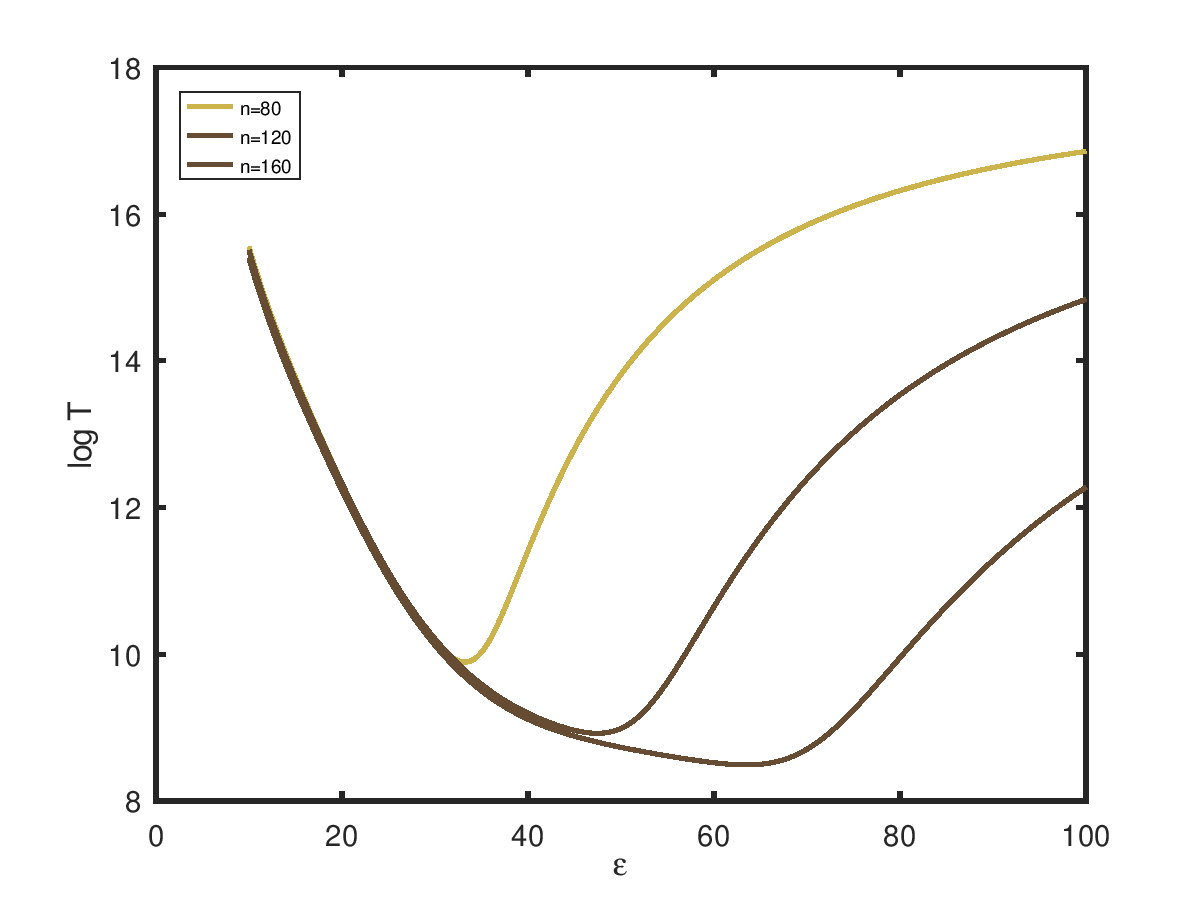
Figure 5: $log(T)$ vs $\varepsilon$ plot to determine the constants of FIR filter.

The smoothened stresses are shown in Fig. 6. Note that the stress components in the solid are different owing to the elastic anisotropy [23].

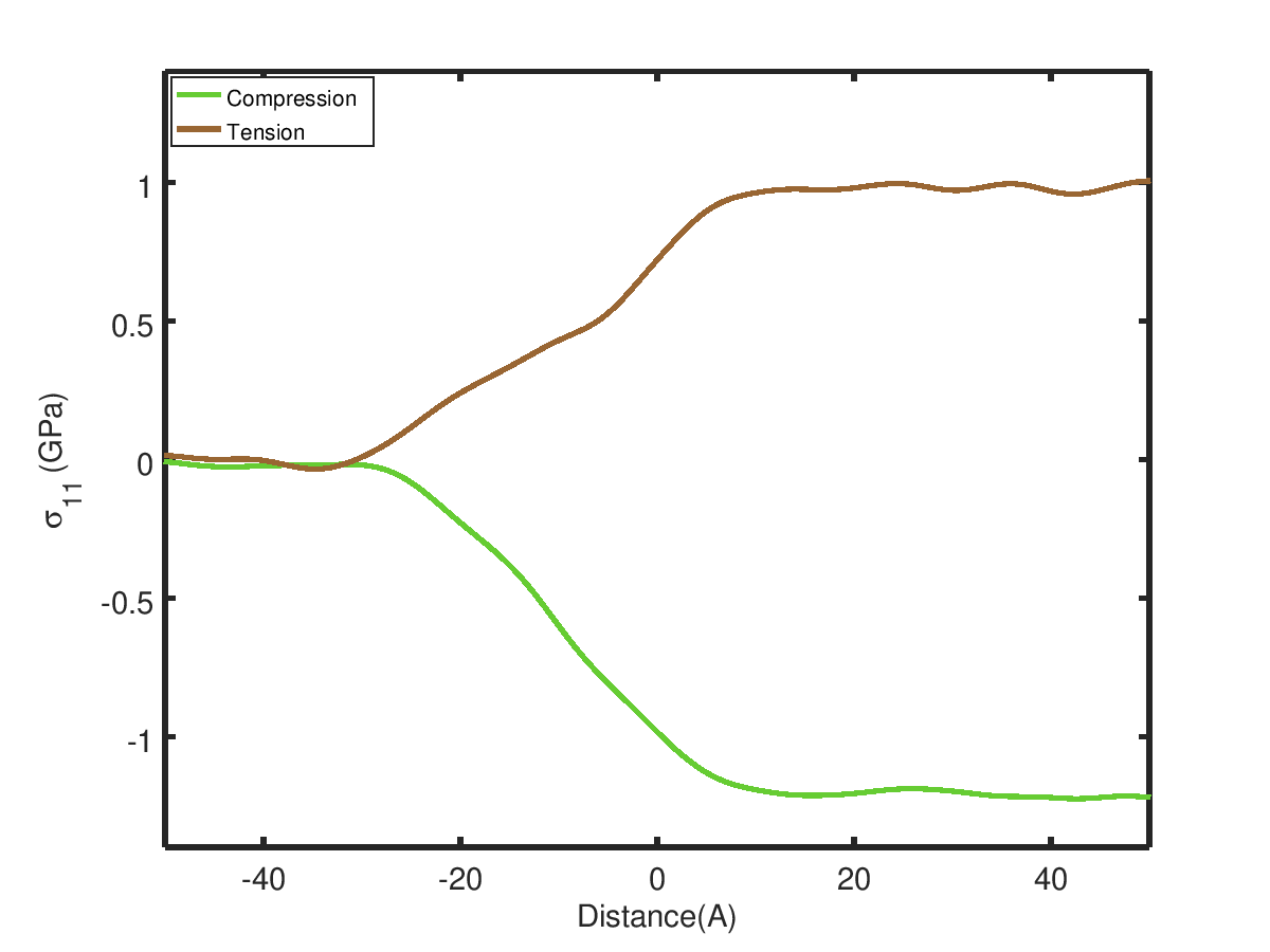
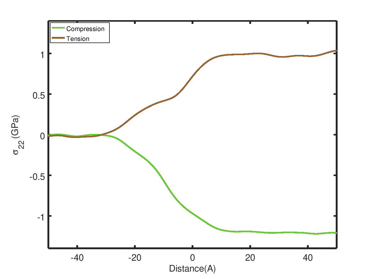
Figure 6: FIR smoothed stress plots of $\sigma_{11}$ and $\sigma_{22}$

As described earlier, the solid is deformed by bi-axial strains in compression and tension, and the resulting interface stress is calculated for each orientation. The interface stress for an isothermal path having interfaces of [001], [110] and [111] orientation for the solid-melt interface are shown in Fig. 7. These results indicate that the interface stress is in the range of -250 mJ/m² to 80 mJ/m² for systems stressed to about 1% biaxially (in compression and tension). Further, in all three cases, in the absence of applied strains, the interface stress is non-zero; for the [001] interface, this stress is tensile ($\approx 8-9$mJ/m²); for [110] and [111] interfaces, the interface stress is compressive (and of the order of 10 and 100 mJ/m², respectively). The interface stress component $\tau_{11}$ and $\tau_{22}$ for [001] and [111] are equal as expected from the symmetry considerations and anisotropy is observed in the case of [110] orientation (that is, the ratio of the stresses deviates from unity). Further, in the unstressed solid, the anisotropy of the interface stress is considerable (0.5) and the anisotropy varies from 0.53 to 0.74. As seen in the case of fcc solids [22], in bcc also we see that the anisotropy changes sign when the imposed strains change from compressive to tensile.

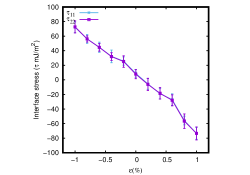
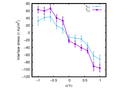
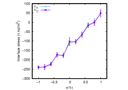
Figure 7: Interface stress components calculated as functions of bi-axial strain for Fe using MD for the interfaces orientated at (a) [001] (b) [110] (c) [111].

4.2 Results from PFC and Amplitude equations

The strain-dependence of interfacial energy and interfacial stress are shown in Fig. 8 and Fig. 9, respectively, for PFC model under isothermal conditions for [001], [110] and [111] orientations. Note that the interfacial stress for PFC model is computed from the strain-dependent interfacial energy based on the Shuttleworth equation, $\tau_{tt}=\gamma+\partial\gamma/\partial\varepsilon_{tt}$. The simulation results are summarized in Table 3 for the PFC model and the AE method.

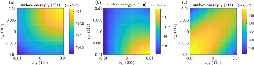
Figure 8: The interfacial energy dependence on in-plane applied strains in PFC model for (a) the [100] orientation, (b) the [110] orientation and (c) the [111] orientation. The color indicates the value of interfacial energy $\gamma$ in the unit of $mJ/m^{2}$. For [001],[110] and [111] orientations, the applied strain $\varepsilon_{11}$ corresponds to [$100$], [$001$] and [$1\bar{1}0$] directions, respectively, while the other applied strain $\varepsilon_{22}$ corresponds to [$010$], [$1\bar{1}0$] and [$11\bar{2}$] directions, respectively.

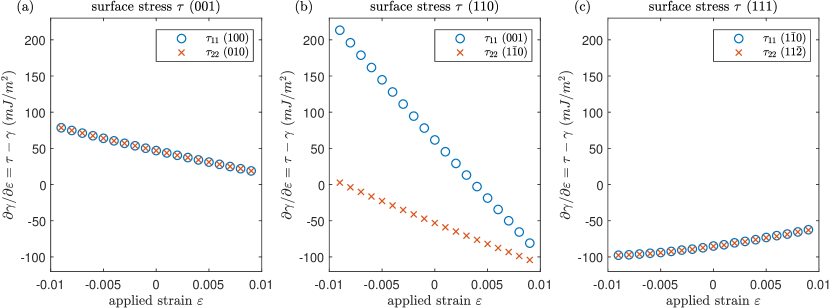
Figure 9: The interfacial stress, $\tau=\partial\gamma/\partial\varepsilon_{tt}$, in PFC model for (a) the [100] orientation, (b) the [110] orientation and (c) the [111] orientation. The surface is subject to the in-plane biaxial strains, namely, $\varepsilon_{11}=\varepsilon_{22}=\varepsilon$.

	$\gamma$ [100]	$\gamma$ [110]	$\gamma$ [111]	$\tau_{11}$ [100]	$\tau_{11}$ / $\tau_{22}$ [110]	$\tau_{11}$ [111]
	($mJ/m^{2}$)	($mJ/m^{2}$)	($mJ/m^{2}$)	($mJ/m^{2}$)	($mJ/m^{2}$)	($mJ/m^{2}$)
PFC	$197.5$	$192.3$	$185.8$	$244.4$	$254.0$ / $139.2$	$100.5$
AE	$188.3$	$183.4$	$177.3$	$219.5$	$224.2$ / $122.3$	$83.4$

Table 3: The interfacial energy $\gamma$ and interfacial stress $\tau$ for strain-free solid ($\varepsilon=0$). The values in the table are presented in the $mJ/m^{2}$ unit for $\gamma$ and $\tau$. Note that $\tau_{11}=\tau_{22}$ for the [100] and [111] orientations due to the lattice symmetry.

4.3 Qualitative and quantitative comparison of results from the three methodologies

As we see from Table. 3, the values of interfacial energies and interface stresses for PFC and the amplitude equations are in good quantitative agreement; specifically, the amplitude equation gives values that are always less than PFC and the difference is about 4.6% to about 17%.

On the other hand, as can be seen from Fig. 10, the MD and PFC/AE are qualitatively similar in most cases; for example, in all cases, the trends are the same in both MD and PFE/AE– namely, for both $(100)$ and $(110)$, the plots show a negative slope while for $(111)$ the plots show a positive slope. However, they are different quantitatively; the range and the nature of the stress (compressive or tensile) is different – even though the order of magnitude is the same, namely, about a couple of hundred mJ/m².

The quantitative differences in the cases of $(110)$ and $(111)$ are the most striking. In MD, for $(110)$, the anisotropy is less for unstressed solid; and, it varies from 0.54 and 0.74 and the nature of anisotropy changes with the change in the nature of imposed strain. In PFC/AE, the tensile imposed strain of about 1% has the least anisotropy (of 0.77) and the compressive imposed strain of about 1% has the highest anisotropy (of 80.38). Interestingly, for the unstressed solid, the anisotropy is very high and is (1.16). Similarly, the differences in slope of the interface stress obtained using MD and that obtained using PFC are very different for the $(111)$ system.

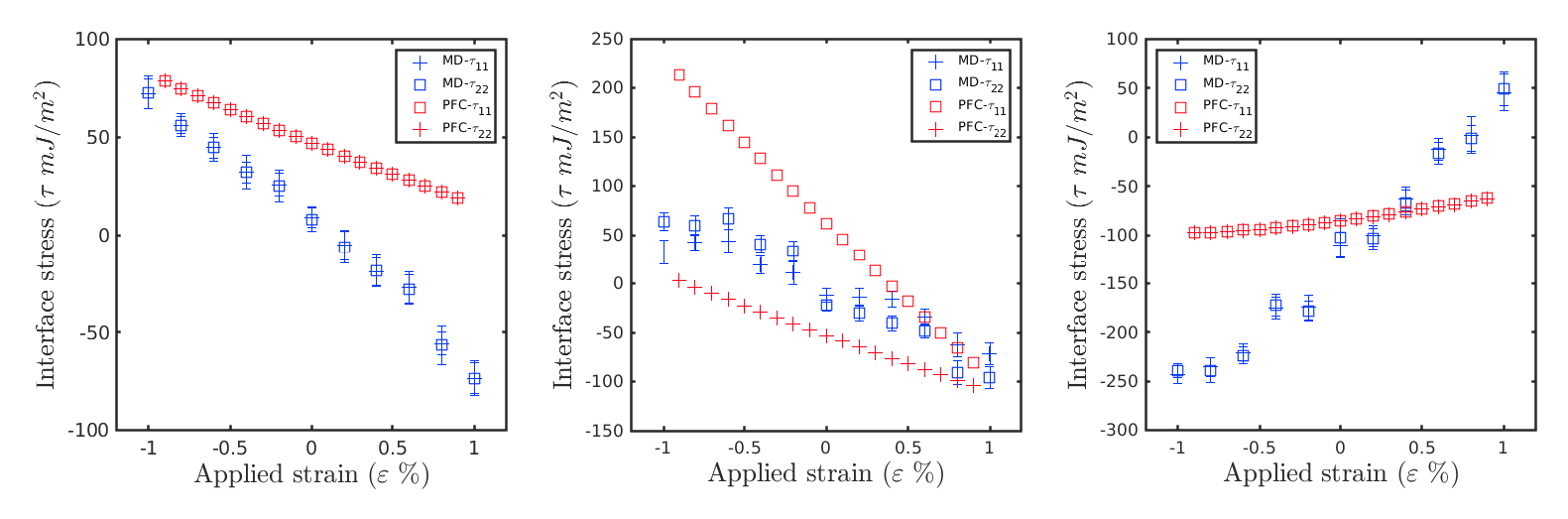
Figure 10: Comparison of the interfacial stress, $\partial\gamma/\partial\varepsilon_{tt}$, obtained in MD and PFC models for (a) the [100] orientation, (b) the [110] orientation and (c) the [111] orientation. The surface is subject to the in-plane biaxial strains, namely, $\varepsilon_{11}=\varepsilon_{22}=\varepsilon$.

In the case of MD, we have used EAM potentials; however, the PFC model employed in this study uses a single parameter to model the system. As shown in previous study, the PFC parameter sets the interface width, and the PFC is shown to predict reasonable interface energy and its anisotropy. However, due to the simplicity of the PFC method, the strain-stress relation of solids are uniquely determined by this parameter at the same time, which may not be realistic. We believe that the discrepancies arise from this difference in the two models, and if the PFC/AE model is modified to capture the elastic moduli more accurately, the quantitative agreement between MD and PFC will improve. Having said that, broadly, for qualitative understanding the anisotropy, the information captures by the PFC model with one parameter (unlike MD which uses EAM potential), is remarkable.

5 Conclusions

We have used both MD and PFC to study the anisotropy in interface stress at the bcc-iron crystal-melt interface. Our results show that the interface stress is anisotropic; this has implications for the equilibrium and growth morphologies of iron particles at the nano-scale. Our study also indicates that with a single parameter, PFC captures the interface stress anisotropy qualitatively and gives stresses at the same order as MD. We also show that the amplitude equations based on PFC can also be used to calculate the interface stresses and the values thus obtained are in good agreement with PFC. Finally, our results show that even in the case of weak anisotropy in interfacial energy, the interface stress anisotropy can be strong.

References

- [1] D. A. Porter, K. E. Easterling, M. Y. Sherif, Phase Transformations in Metals and Alloys, 3rd Edition, CRC Press, 2009.
- [2] D. Turnbull, R. E. Cech, Microscopic observation of the solidification of small metal droplets, Journal of Applied Physics 21 (8) (1950) 804–810. doi:10.1063/1.1699763.
-
[3]
Y. Mishin, M. Asta, J. Li,
Atomistic modeling of
interfaces and their impact on microstructure and properties, Acta
Materialia 58 (4) (2010) 1117–1151.
doi:10.1016/j.actamat.2009.10.049.
URL http://dx.doi.org/10.1016/j.actamat.2009.10.049 - [4] S. Liu, R. E. Napolitano, R. Trivedi, Measurement of anisotropy of crystal-melt interfacial energy for a binary Al-Cu alloy, Acta Materialia 49 (20) (2001) 4271–4276. doi:10.1016/S1359-6454(01)00306-8.
- [5] R. Backofen, A. Voigt, Solid-liquid interfacial energies and equilibrium shapes of nanocrystals, Journal of Physics Condensed Matter 21 (46) (2009). doi:10.1088/0953-8984/21/46/464109.
- [6] R. F. Sekerka, Equilibrium and growth shapes of crystals: How do they differ and why should we care?, Crystal Research and Technology 40 (4-5) (2005) 291–306. doi:10.1002/crat.200410342.
- [7] R. E. Napolitano, S. Liu, R. Trivedi, Experimental measurement of anisotropy in crystal-melt interfacial energy, Interface Science 10 (2-3) (2002) 217–232. doi:10.1023/A:1015884415896.
-
[8]
R. L. Davidchack, B. B. Laird,
Direct
calculation of the hard-sphere crystal melt interfacial free energy,
Phys. Rev. Lett. 85 (2000) 4751–4754.
doi:10.1103/PhysRevLett.85.4751.
URL https://link.aps.org/doi/10.1103/PhysRevLett.85.4751 -
[9]
J. J. Hoyt, M. Asta, A. Karma,
Method for
computing the anisotropy of the solid-liquid interfacial free energy, Phys.
Rev. Lett. 86 (2001) 5530–5533.
doi:10.1103/PhysRevLett.86.5530.
URL https://link.aps.org/doi/10.1103/PhysRevLett.86.5530 - [10] J. J. Hoyt, M. Asta, T. Haxhimali, A. Karma, R. E. Napolitano, R. Trivedi, B. B. Laird, J. R. Morris, Crystal-melt interfaces and solidification morphologies in metals and alloys, MRS Bulletin 29 (12) (2004) 935–939. doi:10.1557/mrs2004.263.
-
[11]
K.-A. Wu, A. Karma,
Phase-field
crystal modeling of equilibrium bcc-liquid interfaces, Phys. Rev. B 76
(2007) 184107.
doi:10.1103/PhysRevB.76.184107.
URL https://link.aps.org/doi/10.1103/PhysRevB.76.184107 -
[12]
A. Jaatinen, C. V. Achim, K. R. Elder, T. Ala-Nissila,
Thermodynamics of
bcc metals in phase-field-crystal models, Phys. Rev. E 80 (2009) 031602.
doi:10.1103/PhysRevE.80.031602.
URL https://link.aps.org/doi/10.1103/PhysRevE.80.031602 -
[13]
G. I. Tóth, N. Provatas,
Advanced
ginzburg-landau theory of freezing: A density-functional approach, Phys.
Rev. B 90 (2014) 104101.
doi:10.1103/PhysRevB.90.104101.
URL https://link.aps.org/doi/10.1103/PhysRevB.90.104101 -
[14]
P. H. Leo, R. F. Sekerka, The effect
of surface stress on crystal melt and crystal crystal equilibrium, Acta
Metallurgica 37 (12) (1989) 3119–3138.
URL <GotoISI>://WOS:A1989CG88000001 - [15] C. Herring, The use of classical macroscopic concepts in surface-energy problems, in: R. Gomer, C. S. Smith (Eds.), Structure and Properties of Solid Surfaces; proceedings of a conference arranged by the National Research Council and held in September, 1952, in Lake Geneva, Wisconsin, USA, Chicago Press, Chicago, 1953, Ch. 1, pp. 5–81.
-
[16]
R. Shuttleworth, The
surface tension of solids, Proceedings of the Physical Society. Section A
63 (5) (1950) 444.
URL http://stacks.iop.org/0370-1298/63/i=5/a=302 - [17] W. C. Johnson, J. I. D. Alexander, Interfacial conditions for thermomechanical equilibrium in two-phase crystals, Journal of Applied Physics 59 (8) (1986) 2735–2746. doi:10.1063/1.336982.
- [18] V. A. Eremeyev, On effective properties of materials at the nano- and microscales considering surface effects, Acta Mechanica 227 (1) (2016) 29–42. doi:10.1007/s00707-015-1427-y.
- [19] K. Momeni, V. I. Levitas, A phase-field approach to nonequilibrium phase transformations in elastic solids: Via an intermediate phase (melt) allowing for interface stresses, Physical Chemistry Chemical Physics 18 (17) (2016) 12183–12203. doi:10.1039/c6cp00943c.
- [20] T. Frolov, Y. Mishin, Temperature dependence of the surface free energy and surface stress: An atomistic calculation for cu(110), Physical Review B 79 (4) (2009). doi:10.1103/PhysRevB.79.045430.
-
[21]
T. Frolov, Y. Mishin, Orientation
dependence of the solid-liquid interface stress: atomistic calculations for
copper, Modelling and Simulation in Materials Science and Engineering 18 (7)
(2010).
URL <GotoISI>://WOS:000282130700004 - [22] T. Frolov, Y. Mishin, Effect of nonhydrostatic stresses on solid-fluid equilibrium. I. bulk thermodynamics, Physical Review B - Condensed Matter and Materials Physics 82 (17) (2010) 1–14. doi:10.1103/PhysRevB.82.174113.
- [23] T. Frolov, Y. Mishin, Effect of nonhydrostatic stresses on solid-fluid equilibrium. II. interface thermodynamics, Physical Review B 82 (17) (2010). doi:10.1103/PhysRevB.82.174114.
- [24] M. W. Liu, K. A. Wu, Investigation of surface/bulk stresses of nanoparticles with diffusive interfaces using the phase field crystal model, Physical Review B 96 (21) (2017). doi:10.1103/PhysRevB.96.214106.
-
[25]
K.-A. Wu, A. Karma, J. J. Hoyt, M. Asta,
Ginzburg-landau
theory of crystalline anisotropy for bcc-liquid interfaces, Phys. Rev. B 73
(2006) 094101.
doi:10.1103/PhysRevB.73.094101.
URL https://link.aps.org/doi/10.1103/PhysRevB.73.094101 - [26] M. I. Mendelev, S. Han, D. J. Srolovitz, G. J. Ackland, D. Y. Sun, M. Asta, Development of new interatomic potentials appropriate for crystalline and liquid iron, Philosophical Magazine 83 (35) (2003) 3977–3994. doi:10.1080/14786430310001613264.
- [27] J. R. Morris, X. Song, The melting lines of model systems calculated from coexistence simulations, Journal of Chemical Physics 116 (21) (2002) 9352–9358. doi:10.1063/1.1474581.
- [28] J. Liu, R. L. Davidchack, H. B. Dong, Molecular dynamics calculation of solid-liquid interfacial free energy and its anisotropy during iron solidification, Computational Materials Science 74 (2013) 92–100. doi:10.1016/j.commatsci.2013.03.018.
- [29] R. Ramakrishnan, R. Sankarasubramanian, Crystal-melt kinetic coefficients of , Acta Materialia 127 (2017) 25–32. doi:10.1016/j.actamat.2017.01.009.
- [30] S. Plimpton, Fast parallel algorithms for short-range molecular dynamics, Journal of Computational Physics 117 (1) (1995) 1–19. doi:10.1006/jcph.1995.1039.
- [31] J. A. Rayne, B. S. Chandrasekhar, Elastic constants of iron from 4.2 to 300°K, Physical Review 122 (6) (1961) 1714–1716. doi:10.1103/PhysRev.122.1714.
-
[32]
S. A. Etesami, E. Asadi,
Molecular dynamics for
near melting temperatures simulations of metals using modified embedded-atom
method, Journal of Physics and Chemistry of Solids 112 (July 2017) (2018)
61–72.
doi:10.1016/j.jpcs.2017.09.001.
URL https://doi.org/10.1016/j.jpcs.2017.09.001 - [33] R. L. Davidchack, J. R. Morris, B. B. Laird, The anisotropic hard-sphere crystal-melt interfacial free energy from fluctuations, Journal of Chemical Physics 125 (9) (2006). doi:10.1063/1.2338303.
- [34] K. R. Elder, M. Katakowski, M. Haataja, M. Grant, Modeling elasticity in crystal growth, Physical Review Letters 88 (24) (2002) 2457011–2457014. arXiv:0107381, doi:10.1103/PhysRevLett.88.245701.
-
[35]
K. R. Elder, M. Grant,
Modeling elastic
and plastic deformations in nonequilibrium processing using phase field
crystals, Phys. Rev. E 70 (2004) 051605.
doi:10.1103/PhysRevE.70.051605.
URL http://link.aps.org/doi/10.1103/PhysRevE.70.051605 -
[36]
N. Pisutha-Arnond, V. W. L. Chan, K. R. Elder, K. Thornton,
Calculations of
isothermal elastic constants in the phase-field crystal model, Phys. Rev. B
87 (2013) 014103.
doi:10.1103/PhysRevB.87.014103.
URL http://link.aps.org/doi/10.1103/PhysRevB.87.014103 -
[37]
V. Heinonen, C. V. Achim, K. R. Elder, S. Buyukdagli, T. Ala-Nissila,
Phase-field-crystal
models and mechanical equilibrium, Phys. Rev. E 89 (2014) 032411.
doi:10.1103/PhysRevE.89.032411.
URL http://link.aps.org/doi/10.1103/PhysRevE.89.032411 -
[38]
K.-A. Wu, P. W. Voorhees,
Stress-induced
morphological instabilities at the nanoscale examined using the phase field
crystal approach, Phys. Rev. B 80 (2009) 125408.
doi:10.1103/PhysRevB.80.125408.
URL https://link.aps.org/doi/10.1103/PhysRevB.80.125408 -
[39]
Y. M. Yu, R. Backofen, A. Voigt,
Morphological
instability of heteroepitaxial growth on vicinal substrates: A phase-field
crystal study, Journal of Crystal Growth 318 (1) (2011) 18–22.
doi:10.1016/j.jcrysgro.2010.08.047.
URL http://dx.doi.org/10.1016/j.jcrysgro.2010.08.047 -
[40]
M. A. Choudhary, J. Kundin, H. Emmerich,
Misfit and
dislocation nucleation during heteroepitaxial growth, Computational
Materials Science 83 (2014) 481–487.
doi:10.1016/j.commatsci.2013.11.030.
URL http://dx.doi.org/10.1016/j.commatsci.2013.11.030 -
[41]
F. Podmaniczky, G. I. Tóth, G. Tegze, T. Pusztai, L. Gránásy,
Phase-field crystal
modeling of heteroepitaxy and exotic modes of crystal nucleation, Journal
of Crystal Growth 457 (2017) 24–31.
doi:10.1016/j.jcrysgro.2016.06.056.
URL http://dx.doi.org/10.1016/j.jcrysgro.2016.06.056 - [42] R. Backofen, A. Voigt, A phase-field-crystal approach to critical nuclei, Journal of Physics Condensed Matter 22 (36) (2010). doi:10.1088/0953-8984/22/36/364104.
- [43] G. Tóth, G. Tegze, T. Pusztai, G. Tóth, L. Gránásy, Polymorphism, crystal nucleation and growth in the phase-field crystal model in 2D and 3D, Journal of Physics Condensed Matter 22 (36) (2010). doi:10.1088/0953-8984/22/36/364101.
- [44] S. Tang, Y. M. Yu, J. Wang, J. Li, Z. Wang, Y. Guo, Y. Zhou, Phase-field-crystal simulation of nonequilibrium crystal growth, Physical Review E - Statistical, Nonlinear, and Soft Matter Physics 89 (1) (2014) 1–6. doi:10.1103/PhysRevE.89.012405.
- [45] K. R. Elder, N. Provatas, J. Berry, P. Stefanovic, M. Grant, Phase-field crystal modeling and classical density functional theory of freezing, Physical Review B - Condensed Matter and Materials Physics 75 (6) (2007) 1–14. doi:10.1103/PhysRevB.75.064107.
-
[46]
K.-A. Wu, A. Adland, A. Karma,
Phase-field-crystal
model for fcc ordering, Phys. Rev. E 81 (2010) 061601.
doi:10.1103/PhysRevE.81.061601.
URL https://link.aps.org/doi/10.1103/PhysRevE.81.061601 -
[47]
M. Greenwood, N. Provatas, J. Rottler,
Free energy functionals
for efficient phase field crystal modeling of structural phase
transformations, Phys Rev Lett 105 (4) (2010) 045702.
doi:10.1103/PhysRevLett.105.045702.
URL https://www.ncbi.nlm.nih.gov/pubmed/20867862 -
[48]
M. Greenwood, J. Rottler, N. Provatas,
Phase-field-crystal
methodology for modeling of structural transformations, Phys Rev E Stat
Nonlin Soft Matter Phys 83 (3 Pt 1) (2011) 031601.
doi:10.1103/PhysRevE.83.031601.
URL https://www.ncbi.nlm.nih.gov/pubmed/21517507 -
[49]
P. Y. Chan, N. Goldenfeld,
Nonlinear
elasticity of the phase-field crystal model from the renormalization group,
Phys. Rev. E 80 (2009) 065105.
doi:10.1103/PhysRevE.80.065105.
URL http://link.aps.org/doi/10.1103/PhysRevE.80.065105 -
[50]
K. R. Elder, Z. F. Huang, N. Provatas,
Amplitude expansion of
the binary phase-field-crystal model, Phys Rev E Stat Nonlin Soft Matter
Phys 81 (1 Pt 1) (2010) 011602.
doi:10.1103/PhysRevE.81.011602.
URL https://www.ncbi.nlm.nih.gov/pubmed/20365379 - [51] R. L. Davidchack, B. B. Laird, Simulation of the hard-sphere crystal–melt interface, The Journal of Chemical Physics 108 (22) (1998) 9452–9462. doi:10.1063/1.476396.
- [52] Y. Bai, Molecular dynamics simulation study of solid-liquid interface properties of HCP magnesium, Master’s thesis, McMaster University, Canada (2012).