Xi et al.

Single-leader multi-follower games for the regulation of two-sided Mobility-as-a-Service markets

Single-leader multi-follower games for the regulation of two-sided Mobility-as-a-Service markets

Haoning Xi School of Civil and Environmental Engineering, UNSW Sydney, NSW, 2052, Australia.
Data61, CSIRO, Canberra ACT 2601, Australia.
Didier Aussel PROMES UPR CNRS 8521, Université de Perpignan Via Domitia, Tecnosud, 66100 Perpignan, France.
Wei Liu School of Civil and Environmental Engineering, UNSW Sydney, NSW, 2052, Australia.
School of Computer Science and Engineering, University of New South Wales, Sydney, NSW 2052, Australia.
S.Travis Waller School of Civil and Environmental Engineering, UNSW Sydney, NSW, 2052, Australia.
David Rey SKEMA Business School, Université Côte d’Azur, Sophia Antipolis Campus, France.
School of Civil and Environmental Engineering, UNSW Sydney, NSW, 2052, Australia.
david.rey@skema.edu

Mobility-as-a-Service (MaaS) is an emerging business model driven by the concept of “Everything-as-a-Service” and enabled through mobile internet technologies. In the context of economic deregulation, a MaaS system consists of a typical two-sided market, where travelers and transportation service providers (TSPs) are two groups of agents interacting with each other through a MaaS platform. In this study, we propose a modeling and optimization framework for the regulation of two-sided MaaS markets. We consider a name-your-own-price (NYOP)-auction mechanism where travelers submit purchase-bids to accommodate their travel demand via MaaS platform, and TSPs submit sell-bids to supply mobility resources for the MaaS platform in exchange for payments. We cast this problem as a single-leader multi-follower game (SLMFG) where the leader is the MaaS regulator and two groups of follower problems represent the travelers and the TSPs. The MaaS regulator aims to maximize its profits by optimizing operations. In response to the MaaS regulator’s decisions, travelers (resp. TSPs) adjust their participation level in the MaaS platform to minimize their travel costs (resp. maximize their profits). We analyze cross-group network effects in the MaaS market, and formulate SLMFGs without and with network effects leading to mixed-integer linear bilevel programming and mixed-integer quadratic bilevel programming problems, respectively. We propose customized branch-and-bound algorithms based on strong duality reformulations to solve these SLMFGs. Extensive numerical experiments conducted on large scale simulation instances generated from realistic mobility data highlight that the performance of the proposed algorithms is significantly superior to a benchmarking approach, and provide meaningful managerial insights for the regulation of two-sided MaaS markets in practice.

Mobility-as-a-Service, Two-sided markets, Single-leader multi-follower games, Bilevel optimization, Branch-and-Bound.

1 Introduction

The accelerated evolution of the digital and shared economies in recent years has brought profound shifts in how various services are delivered. In this context, the transportation industry is undergoing a massive revolution from infrastructure-focused towards service-focused business models brought by the “Mobility-as-a-Service (MaaS)” concept. According to the MaaS Alliance (MaaS 2020), MaaS integrates various forms of transportation services into a single mobility service accessible on demand. To meet a traveler request, the MaaS operator can provide a diverse combination of mobility options across multiple travel modes, including public transport, ride-, car- or bike-sharing, taxi; hereby referred to as a MaaS bundle. MaaS is a user-centric framework where customized services and mode-agnostic mobility resources are priced in a unified framework. Yet, in the vast majority of studies on MaaS systems, mobility resource pricing is based on segmented travel modes. Xi et al. (2020) made an initial attempt to address this research gap by introducing innovative MaaS mechanisms where users can bid for any quantity of mobility resources in a mode-agnostic fashion with preference requirements, and the MaaS regulator allocates the mobility resources integrated from various transportation service providers (TSPs) to meet heterogeneous traveler requests. In this MaaS framework, the mobility service provided by different travel modes are unified as mobility resources with continuous provision by capturing the travel distance and the average service speed. Building on this flexible MaaS framework, we consider a MaaS system under economic deregulation (Wong et al. 2020), which admits a natural two-sided market representation wherein a MaaS regulator aims to promote the participation of both travelers and TSPs. The operation of a two-sided MaaS market is challenging due to the interactions among different stakeholders, i.e. the regulator, travelers and TSPs which may have divergent and conflicting objectives (Meurs and Timmermans 2017). To capture the interactions across stakeholders of a two-sided MaaS market, we propose a single-leader multi-follower game (SLMFG) where the MaaS regulator is the leader, travelers and TSPs are two groups of followers. In the proposed SLMFG, the MaaS regulator makes operational decisions, i.e., price, MaaS bundles, to allocate mobility resources to travelers, maximizing its profits by anticipating the participation of followers. Each traveler aims to minimize her travel costs by deciding the participation level defined as the proportion of mobility demand fulfilled through the MaaS platform in comparison with outside options. Each TSP aims to maximize its profits by deciding the participation level defined as the proportion proportion of mobility resources supplied to the MaaS platform in comparison with its reserve options. Two-sided markets represent a refinement of the concept of cross-group network effects, which is captured by the supply-demand gap in this study. We formulate SLMFGs without and with network effects which lead to mixed-integer linear bilevel programming (MILBP) and mixed-integer quadratic bilevel programming (MIQBP) problems with multiple constraints representing followers’ strategies, respectively. Then we propose exact solution methods to find optimal solutions for both MILBP and MIQBP problems.

We next review the literature on two-sided markets in flexible mobility systems (Section 1.1), single-leader multi-follower games (Section 1.2), solution approaches of bilevel programming problems (Section 1.3) and outline the main contributions of this paper (Section 1.4).

1.1 Two-sided markets in flexible mobility systems

A two-sided market is one in which two groups of agents interact through a platform, and the decisions of each group of agents affect the outcomes of the other group of agents, typically through an externality (Rysman 2009). The goal of the platform regulator is to incentivize the participation of both sides of the market (Rochet and Tirole 2003). Two-sided platforms have become omnipresent in literature on flexible mobility systems, especially for pricing in ridesourcing markets. Wang et al. (2016) introduced matching mechanisms to model the cross-group externalities between customers and taxi drivers on an e-hailing platform and reveal the impacts of the pricing strategy of an e-hailing platform in taxi service. Djavadian and Chow (2017) explored MaaS in the framework of two-sided markets based on agent-based stochastic, day-to-day adjustment processes using Ramsey’s pricing criterion for social optimum. Bai et al. (2019) examined how various factors affect the optimal price, wage, and commission by considering heterogeneous earning-sensitive drivers and price-sensitive passengers. Nourinejad and Ramezani (2020) introduced a dynamic model in a two-sided ridesourcing market such that supply and demand are endogenously dependent on the fare charged from riders, the wage paid to drivers, riders’ waiting time and drivers’ cruising time. He et al. (2021) proposed an integrated model of two-sided platforms by addressing the joint design of incentives and spatial capacity allocations in shared-mobility systems.

1.2 Single-leader multi-follower games

Single-leader multi-follower games (SLMFGs) can be viewed as a particular class of hierarchical decision problems belonging to the class of bilevel optimization (Dempe 2002). SLMFGs have a various of practical applications in operations and management. Wu et al. (2016) developed a leader-follower game model to evaluate the potential gains from the merger of different organizations with constrained resources and discussed its applications in banking operations. Zha et al. (2018) investigated the performance of surge pricing in ridesharing system where the leader’s problem determines the prices and the followers’ problem represents drivers’ equilibrium in work hour choices. Rey et al. (2019) considered the network maintenance problem, where the leader problem describes the manager’s policy problem and each lower level problem represents a user equilibrium problem per time period. Xiong et al. (2021) investigated a resource recovery planning problem where the local authority (leader) solves a joint waste and cost sharing problem to minimize its expected payout, and each private operator (follower) solves a facility location and resource recovery operations problem to maximize its expected total profits.

1.3 Solution approaches for bilevel optimization problems

Solving bilevel optimization problems is a challenging task since even the linear single-leader single-follower problems are NP-hard (Bard 1991). The most common solution approach for linear bilevel programming (LBP) problems is to replace the lower-level problem with its Karush-Kuhn-Tucker (KKT) conditions, leading to a Mathematical Program with Equilibrium Constraints (MPEC) (Luo et al. 1996). Fortuny-Amat and McCarl (1981) proposed to reformulate the complementary slackness condition by introducing a large positive constant $M$ and a binary variable, thus converting LBPs into large mixed-integer programming problems. This approach has been studied in several papers, e.g., Luathep et al. (2011), Dempe and Zemkoho (2012). However, since the MPEC reformulation of LBPs require binary variables for each complementary slackness condition, this may affect computational scalability. To address this drawback, an alternative method is to employ the strong-duality (SD) property of linear programming to reformulate a linear lower-level using a primal-dual inequality (Pandzic et al. 2012, Beheshti et al. 2016). Zare et al. (2019) compared the performance of SD-based reformulations against KKT-based ones and showed that the SD-based approaches could reduce computational runtime by several orders of magnitude for certain classes of instances. In contrast to the MPEC reformulation, the number of additional binary variables in SD-based reformulations does not depend on the size of the follower’s problem. Further, if the leader variables interacting with the follower problem are integers, the resulting nonlinear constraints induced by the SD reformulation can be linearized by applying classical linearization approaches for integer-linear bilinear terms such as so-called big-$M$ approaches (Glover and Woolsey 1974, Liberti et al. 2009). However, Pineda and Morales (2019) raised concerns about the widespread use of big-$M$ approaches to solve LBP and showed that the heuristic procedure employed to select the big-$M$ in many published works may actually fail and provide suboptimal solutions. Kleinert et al. (2020a) considered the hardness to find a correct big-$M$ for LBP and showed that identifying such value is NP-hard.

To obviate the aforementioned issues induced by follower-problem mixed-integer reformulations, exact algorithms based on branch-and-bound (B&B) have been developed (Falk and Soland 1969, Bard and Falk 1982). Bard and Moore (1990) developed a B&B algorithm based on the MPEC reformulation, referred to as $\mathsf{Bard\&Moore}$ in this paper, which works by relaxing nonlinear constraints corresponding to complementary slackness conditions and branching on these constraints. However, this approach may require a substantial amount of branching on complementary conditions which may be impractical on large problems. Recently, Kleinert et al. (2020b) derived valid inequalities for LBP by exploiting the SD conditions of the follower-level problem, which proves to be very effective in closing the gap for some instances.

The above review of the literature highlights that solving bilevel optimization problem is highly non-trivial, even in the single-follower case. Using big-$M$ approaches may fail and provide suboptimal solutions, thus it is necessary to develop exact solution approaches.

1.4 Our contributions

In this study, we present a novel approach for the regulation of two-sided MaaS markets. We propose a SLMFG where the MaaS regulator is the leader while travelers and TSPs are represented as two groups of multiple followers. The proposed SLMFG aims to capture the interaction of all three types of stakeholders (MaaS regulator, travelers and TSPs). The main contributions of this study are summarized as follows:

• We develop a name-your-own-price (NYOP) auction-based mechanism for two-sided MaaS markets which allows travelers and TSPs to submit heterogeneous MaaS requests, including their preference and willingness to pay/sell in terms of purchase/sell-bids simultaneously.

• We formulate the SLMFG revealing the hierarchical interactions between the MaaS regulator (the leader) and the travelers/TSPs (the followers) through the pricing strategies and MaaS bundles, as well as the cross network effects between travelers and TSP by tracking the supply and demand in the two-sided MaaS markets. Specifically, we formulate SLMFGs without and with network effects leading to MILBP and MIQBP problems, respectively.

• We provide constraint qualifications for MPEC reformulations and theoretically prove the equivalence between proposed SLMFGs and their MPEC reformulations.

• We propose a new exact solution approach to solve the proposed SLMFGs that combines SD reformulation with a customized branch-and-bound algorithm, referred to as $\mathsf{SD}$-$\mathsf{B\&B}$. We conduct extensive numerical experiments which highlight that the proposed algorithm ($\mathsf{SD}$-$\mathsf{B\&B}$) considerably outperforms the classical B&B algorithm ($\mathsf{Bard\&Moore}$) and draw managerial insights that can be used as operational management guidelines in practice.

To the best of our knowledge, this is the first tractable framework where single-leader multi-follower game approach is used for modelling a two-sided MaaS market and the first SD-based branch and bound algorithm with customized branching rules for solving both MILBP and MIQBP problems.

The rest of this paper is organized as follows: Section 2 gives the problem description; Section 3 introduces SLMFGs in the two-sided MaaS market; Section 4 introduces the exact solution methods for the SLMFGs; Section 5 presents the computational study; Section 6 concludes the study and discusses future research directions.

2 Problem description

This section introduces preliminaries and notations (Section 2.1), presents the NYOP-auction mechanism (Section 2.2) and provides an overview of the SLMFG (Section 2.3).

2.1 Preliminaries and Notations

In this study, we take the perspective of a MaaS regulator who aims to make the optimal operational strategies, i.e., pricing policy, and allocate mobility resources integrated from TSPs to travelers in terms of multi-modal MaaS bundles in a two-sided MaaS system. In this MaaS framework, the average speed of the travel modes is assumed known and representative of the “Commercial speed” , which incorporates service delays, e.g. waiting time, transfer time, operational stop time as well as the average driving speed. In addition, to quantify the “user experience” of a multi-modal trip, each travel mode is assigned an inconvenience cost per unit of time which aims to capture discomfort in shared mobility modes and is dependent on the vehicle occupancy (the number of shared riders on a vehicle), e.g., inconvenience cost per unit time of taxi is smaller than that of public transit. Travelers can request total service time and the corresponding willingness to pay for each trip, they are also required to submit the personal information while registering for the MaaS platform, such as inconvenience tolerance and travel delay budget representing the maximum acceptable inconvenience cost and delay for a mobility service.

To quantify the mobility services consisting of different travel modes, we introduce the quantity of mobility resource defined as speed-weighted travel distance. Let $D_{i}$ and $T_{i}$ denote Traveler $i$’s requested travel distance and total service time, the corresponding mobility resources are defined as $Q_{i}\triangleq\frac{D_{i}}{T_{i}}D_{i}$, where $\frac{D_{i}}{T_{i}}$ denotes Traveler $i$’s requested average service speed. Using this concept, users’ MaaS requests are converted into mobility resources which can be fulfilled through a multi-modal MaaS bundle with the required commercial speed (service time).

Since TSPs are limited in mobility resource capacity, we assume that mobility capacity of the network is known and can be expressed in terms of mobility resources. We assume that heterogeneous users have preferences towards mobility services such as travelling distance, total service time, inconvenience cost, travel delay and willingness to pay (WTP), and heterogeneous TSPs have preferences towards the capacity of mobility resources and willingness to sell (WTS).

2.2 NYOP-auction mechanism

MaaS aims to deliver a portfolio of multi-modal mobility services that places user experience at the centre of the offer. Thus we propose a name-your-own-price (NYOP) auction-based mechanism, where the user determines the price by submitting a bid and the auctioneer can either accept or reject the user by comparing with an internal threshold price which is invisible for users (Spann et al. 2004). Terwiesch et al. (2005) indicated that the NYOP auction provides a niche market where consumers are sensitive to price or psychologically prefer this type of auction. Cai et al. (2009) evaluated the optimal reserve prices in the NYOP channel with bidding options in various situations. However, since consumers do not have complete information of the products, the existing NYOP auctions are opaque, and consumers have to trade off their convenience with the low price. In order to solve this issue, travelers and TSPs are allowed to submit their heterogeneous preference and WTP/WTS in terms of purchase/sell-bids in the proposed user-centric MaaS system.

Let $\mathcal{I}$ denote the set of travelers, $\mathcal{M}$ denote the set of travel modes and $\mathcal{N}_{m}$ denotes the set of TSPs of mode $m$, $\forall m\in\mathcal{M}$. For each traveler $i\in\mathcal{I}$, the purchase-bid $\mathcal{B}_{i}=(D_{i},T_{i},b_{i},B_{i},R_{i},\Gamma_{i})$ is defined as a tuple consisting of the following data: $D_{i}$ is Traveler $i$’s requested travel distance, $T_{i}$ is Traveler $i$’s requested total service time, $b_{i}$ is Traveler $i$’s unit purchase-bidding price (WTP), $B_{i}$ is Traveler $i$’s travel expenditure budget, $R_{i}$ is Traveler $i$’s travel delay budget and $\Gamma_{i}$ is Traveler $i$’s inconvenience tolerance. For each TSP $mn$, $m\in\mathcal{M},n\in\mathcal{N}_{m}$, its sell-bid $\mathcal{B}_{mn}=(C_{mn},\beta_{mn},\bar{B}_{mn})$ is defined as a tuple, where $C_{mn}$ is the capacity of TSP $mn$ in terms of quantity of mobility resources, $\beta_{mn}$ is TSP $mn$’s unit sell-bidding price (WTS) and $\bar{B}_{mn}$ is TSP $mn$’s operating cost budget.

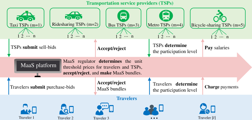
Figure 1: NYOP auction-based mechanism in the two-sided MaaS market

Given the purchase/sell-bids of travelers/TSPs, The MaaS regulator solves a SLMFG to determine the unit threshold price for travelers and TSPs, respectively, allocate mobility resources to users in terms of MaaS bundles, so as to maximize its profits while coordinating travelers’ mobility demand and the mobility resources supplied by TSPs. On the one hand, if a traveler’s WTP on per unit mobility is higher than or equal to the unit threshold price for travelers, she will be accepted; otherwise, she will be rejected. On the other hand, if a TSP’s WTS on per unit mobility is lower than or equal to the unit threshold price for TSPs, it will be accepted, otherwise, it will be rejected by the MaaS regulator. More details on the SLFMG are provided in Section 2.3. Considering five travel modes, the proposed NYOP auction process is also illustrated in Figure 1.

2.3 SLMFG model overview

We propose a SLMFG where the MaaS regulator is the leader, while travelers and TSPs are two groups of followers. We next introduce the main decision variables of the SLMFG before discussing cross network effects. A summary of the parameters, variables and sets used in the mathematical models is provided in Table 3 of Online Appendix 7.

2.3.1 Decision variables.

In the proposed NYOP mechanism, we denote $p$ and $q$ the non-negative real variable representing the unit threshold price for travelers and TSPs, respectively. Then the MaaS regulator accepts or rejects participants by comparing their bidding prices with the internal threshold unit price. We denote $u_{i}\in\{0,1\}$ the binary variable indicating whether the MaaS regulator accepts traveler $i$, $\forall i\in\mathcal{I}$, to join the MaaS platform (1) or not (0). Analogously, we denote $w_{mn}\in\{0,1\}$ the binary variable indicating whether the MaaS regulator accepts TSP $mn$, $\forall m\in\mathcal{M},n\in\mathcal{M}_{n}$, to join the MaaS platform (1) or not (0). In the proposed SLMFG, the travelers/TSPs decide whether to join the MaaS platform or not, and to which extent they wish to use/supply the MaaS platform. Note that $u_{i}=1$ (resp. $w_{mn}=1$) only means that traveler $i$ (resp. TSP $mn$) has the option to join the MaaS platform, i.e., if a traveler is accepted by the MaaS regulator, she may join the MaaS platform with a certain participation level or not join the MaaS platform. However, $u_{i}=0$ (resp. $w_{mn}=0$) means that traveler $i$ (resp. TSP $mn$) cannot join the MaaS platform.

The allocation of mobility resources supplied by TSPs to travelers is coordinated via real variables $l_{i}^{m}\geq 0$, which represent the service time of travel mode $m\in\mathcal{M}$ in the MaaS bundle of Traveler $i\in\mathcal{I}$. Cross network effects in the two-sided market are captured by the real variable $\Delta$ which represents the supply-demand gap based on the decisions of followers (more details are provided in Section 2.3.2). The decision space of the leader is thus the tuple $(p,q,\bm{u},\bm{w},\bm{l},\Delta)$ where bold-face symbols represent vectors of variables of appropriate dimensions.

The decision variables of followers are divided into two groups of variables $\bm{x}=[x_{i}]_{i\in\mathcal{I}}$ for travelers and $\bm{y}=[y_{mn}]_{m\in\mathcal{M},n\in\mathcal{N}_{m}}$ for TSPs. For each traveler $i\in\mathcal{I}$, $x_{i}\in[0,1]$ is a real variable representing the proportion of mobility demand that $i$ decides to use the MaaS platform in comparison with her other options, e.g., private vehicles and public transit. Analogously, for each TSP $mn$, $m\in\mathcal{M},n\in\mathcal{N}_{m}$, $y_{mn}\in[0,1]$ is a real variable representing the proportion of mobility resources that TSP $mn$ decides to supply the MaaS platform as opposed to its reserve options. Hereby $x_{i}$ and $y_{mn}$ are referred to as Traveler $i$’s and TSP $mn$’s participation level on MaaS platform, respectively.

2.3.2 Cross network effects.

Cross network effects aim to capture the interaction between both sides of the MaaS market. E.g., an increase in the mobility resources supplied by TSPs will reduce travelers’ average waiting time and may thus increase their travel demand. Reciprocally, a decrease of travelers’ mobility demand for MaaS may increase TSPs’ average idle time and thus disincentivize participation. We propose to capture these cross network effects through the supply-demand gap in the two-sided MaaS market.

Recall that Traveler $i$’s total demand is $Q_{i},\forall i\in\mathcal{I}$, and TSP $mn$’s maximum supply is $C_{mn},\forall m\in\mathcal{M},n\in\mathcal{N}_{m}$. Travelers’ total demand on MaaS is written as $\sum_{i\in\mathcal{I}}Q_{i}x_{i}$ and TSPs’ total supply is written as $\sum_{m\in\mathcal{M}}\sum_{n\in\mathcal{N}_{m}}C_{mn}y_{mn}$. The supply-demand gap in the MaaS market is given in Eq.(1):

$$\Delta=\sum_{m\in\mathcal{M}}\sum_{n\in\mathcal{N}_{m}}C_{mn}y_{mn}-\sum_{i\in\mathcal{I}}Q_{i}x_{i}.$$ (1)

The range of $\Delta$ is $[\underline{C},\overline{C}]$, where $\underline{C}$ is the reserved capacity of the MaaS regulator and $\overline{C}$ is the capacity of mobility resources provided by all TSPs, namely, $\overline{C}=\sum_{m\in\mathcal{M}}\sum_{n\in\mathcal{N}_{m}}C_{mn}$.

Let $\Delta_{-i}$ and $\Delta_{-mn}$ denote the supply-demand gap perceived by Traveler $i$ and TSP $mn$, which are defined in (2) and (3), respectively,

$$\Delta_{-i}=\sum_{m\in\mathcal{M}}\sum_{n\in\mathcal{N}_{m}}C_{mn}y_{mn}-(\sum_{i\in\mathcal{I}}Q_{i}x_{i}-Q_{i}x_{i})=\Delta+Q_{i}x_{i},$$ (2)

$$\Delta_{-mn}=(\sum_{m\in\mathcal{M}}\sum_{n\in\mathcal{N}_{m}}C_{mn}y_{mn}-C_{mn}y_{mn})-\sum_{i\in\mathcal{I}}Q_{i}x_{i}=\Delta-C_{mn}y_{mn},$$ (3)

It is widely accepted that traveler’s waiting time and TSP’s idle time are highly dependent on the supply of participating TSPs and demand of participating travelers, e.g., Bai et al. (2019). We assume that the MaaS regulator estimates travelers’ average waiting time and TSPs’ average idle time based on the supply-demand gap $\Delta$. These estimated average waiting/idle time are reported to travelers/TSPs. We assume that, in the long run, Traveler $i$ (resp. TSP $mn$) observes $\Delta$ based on the estimated waiting (resp. idle) time information provided by the MaaS regulator, and perceives average waiting (resp. idle) time as functions of $\Delta_{-i}$ (resp. $\Delta_{-mn}$), and then use this perceived time information to make their own decisions.

As Traveler $i$’s perceived supply-demand gap ($\Delta_{-i}$) increases, her perceived average waiting time decreases. Similarly, as TSP $mn$’s perceived supply-demand gap ($\Delta_{-mn}$) increases, her perceived average idle time increases. Let $\Psi_{i}(x_{i},\Delta)$ denote the perceived waiting time function of traveler $i\in\mathcal{I}$ and $\Phi_{mn}(y_{mn},\Delta)$ denote the perceived idle time of TSP $mn$, $m\in\mathcal{M},n\in\mathcal{N}_{m}$. We consider two types of perceived waiting/idle time functions for travelers/TSPs: linear and quadratic.

Linear waiting/idle functions of Traveler $i$/TSP $mn$ are given in Eq.(4a)/Eq.(4b).

$$\text{Traveler $i$'s perceived waiting time}:\quad\Psi_{i}^{l}(x_{i},\Delta)=-\frac{\zeta}{\overline{C}}(\Delta+Q_{i}x_{i})+\vartheta,$$ (4a)

$$\text{TSP $mn$'s perceived idle time}:\quad\Phi_{mn}^{l}(y_{mn},\Delta)=\frac{\kappa}{\overline{C}}(\Delta-C_{mn}y_{mn})+\xi,$$ (4b)

Quadratic waiting/idle functions of Traveler $i$/TSP $mn$ are given in Eq.(5a)/Eq.(5b).

$$\text{Traveler $i$'s perceived waiting time}:\Psi_{i}^{q}(x_{i},\Delta)=\frac{\zeta}{\overline{C}^{2}}(\Delta+Q_{i}x_{i})^{2}-\frac{2\zeta}{\overline{C}}(\Delta+Q_{i}x_{i})+\vartheta,$$ (5a)

$$\text{TSP $mn$'s perceived idle time}:\quad\Phi_{mn}^{q}(y_{mn},\Delta)=\frac{\kappa}{\overline{C}^{2}}(\Delta-C_{mn}y_{mn})^{2}+\xi.$$ (5b)

In Eq.(4)-(5), $\zeta$, $\kappa$, $\vartheta$ and $\xi$ are positive parameters which ensure that perceived waiting/idle time functions are nonnegative. Observe that if $\Delta+Q_{i}x_{i}\in[0,\overline{C}]$, then $\Psi_{i}^{l}(x_{i},\Delta)$ and $\Psi_{i}^{q}(x_{i},\Delta)$ are strictly monotone decreasing with regards to $\Delta$ and satisfy $\Psi_{i}^{l}(x_{i},\Delta),\Psi_{i}^{q}(x_{i},\Delta)\in[\vartheta-\zeta,\vartheta]$. Analogously, if $\Delta-C_{mn}y_{mn}\in[0,\overline{C}]$, then $\Phi_{mn}^{l}(y_{mn},\Delta)$ and $\Phi_{mn}^{q}(y_{mn},\Delta)$ are strictly monotone increasing with regards to $\Delta$ and satisfy $\Phi_{mn}^{l}(y_{mn},\Delta),\Phi_{mn}^{q}(y_{mn},\Delta)\in[\xi,\kappa+\xi]$.

The proposed SLMFG model for two-sided MaaS markets is illustrated in Figure 2. The MaaS regulator aims to maximize profits by adjusting the unit threshold price for travelers ($p$) and the unit threshold price for TSPs ($q$), as well as making MaaS bundles ($\bm{l}$), while anticipating the choices of followers on participation levels of the MaaS platform. On the one hand, each traveler aims to minimize her travel costs by choosing the proportion of their mobility demand ($x_{i}$) fulfilled via the MaaS platform. On the other hand, TSPs aim to maximize its profits by choosing the proportion of their mobility resources ($y_{mn}$) supplied to the MaaS platform. The “supply” of participating TSPs and the “demand” of travelers’ requests are endogenously dependent on the unit threshold price set by the leader and other followers’ decisions. The network effects information is captured by travelers’ perceived waiting time and TSPs’ perceived idle time, both of which are functions of the supply-demand gap $\Delta$. As $\Delta$ increases, travelers’ perceived waiting time will decrease and TSPs’ perceived idle time will increase. Thus, in the proposed two-sided MaaS market, the participation levels of travelers (resp. TSPs) is affected by the participation levels of TSPs (resp. travelers).

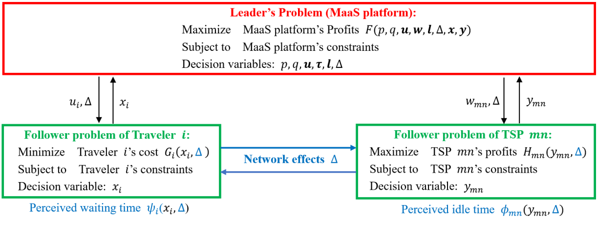
Figure 2: Overview of the SLMFG model in the two-sided MaaS markets

3 SLMFG formulations for two-sided MaaS markets

In this section, we introduce SLMFG formulations in Section 3.1, the SLMFG base formulation in Section 3.2, and dedicate SLMFG formulations with and without network effects in Section 3.3.

3.1 SLMFG formulations

We first introduce two follower problems before presenting the leader problem.

3.1.1 Follower problems.

We consider two groups of follower problems, one per side of the two-sided MaaS market, i.e., travelers and TSPs.

Travelers’ problem: The objective of travelers is to minimize their total travel costs. For each traveler $i\in\mathcal{I}$, let $r_{i}$ denote Traveler $i$’s unit reserve price and $\alpha_{i}$ denotes Traveler $i$’s unit waiting time cost. The travel cost of Traveler $i$ include travel cost for using the MaaS platform, travel cost for her reserve travel options, and the perceived waiting time cost $\alpha_{i}\Psi_{i}(x_{i},\Delta)$. The objective function of traveler’s problem is denoted by $G_{i}(x_{i},\Delta)$ and given in Eq.(T.1).

$$\min_{x_{i}}\quad\underbrace{G_{i}(x_{i},\Delta)}_{\text{Total travel cost}}=\underbrace{b_{i}Q_{i}x_{i}}_{\text{MaaS travel cost}}+\underbrace{r_{i}Q_{i}(1-x_{i})}_{\text{reserve travel cost}}+\underbrace{\alpha_{i}\Psi_{i}(x_{i},\Delta)}_{\text{waiting time cost}}.$$ (T.1)

Recall that $B_{i}$ is Traveler $i$’s travel expenditure budget for using MaaS, hence we require:

$$b_{i}Q_{i}x_{i}\leq B_{i}.$$ (T.2)

To capture accept/reject decisions of the MaaS regulator in the strategy of Traveler $i$, leader variable $u_{i}$ is introduced as an upper bound for $x_{i}$, i.e.,

$$x_{i}\leq u_{i},$$ (T.3)

$$x_{i}\geq 0.$$ (T.4)

In sum, the follower problem of Traveler $i\in\mathcal{I}$ consists of Eqs.(T.1)-(T.4).

TSPs’ problem: The objective of TSPs is to maximize their profits. For any $m\in\mathcal{M}$ and $n\in\mathcal{N}_{m}$, let $\gamma_{mn}$ denote TSP $mn$’s unit operating cost, $\rho_{mn}$ denote TSP $mn$’s unit reserve price, and $\eta_{mn}$ denote TSP $mn$’s unit idle time cost. Recall that $\beta_{mn}$ is the unit sell-bidding price of TSP $mn$. The objective function of TSP $mn$ is denoted $H_{mn}(y_{mn},\Delta)$ and given in Eq.(P.1):

$$\max_{y_{mn}}\hskip 9.95863pt\underbrace{H_{mn}(y_{mn},\Delta)}_{\text{Total profits}}=\underbrace{\left(\beta_{mn}-\gamma_{mn}\right)C_{mn}y_{mn}}_{\text{revenue from MaaS}}+\underbrace{(\rho_{mn}-\gamma_{mn})C_{mn}(1-y_{mn})}_{\text{revenue from reserve options}}-\underbrace{\eta_{mn}\Phi_{mn}(y_{mn},\Delta)}_{\text{idle time cost }}.$$ (P.1)

Recall that $\bar{B}_{mn}$ is TSP $mn$’s operating cost budget for supplying the MaaS platform, we require:

$$C_{mn}\gamma_{mn}y_{mn}\leq\bar{B}_{mn}.$$ (P.2)

To capture accept/reject decisions of the MaaS platform in the strategy of TSP $mn$, leader variable $w_{mn}$ is introduced as an upper bound for $y_{mn}$, i.e.:

$$y_{mn}\leq w_{mn},$$ (P.3)

$$y_{mn}\geq 0.$$ (P.4)

In sum, the follower problem of TSP $mn$, $m\in\mathcal{M},n\in\mathcal{N}_{m}$ consists of Eqs.(P.1)-(P.4).

3.1.2 Leader’s problem.

The objective of the MaaS regulator is to maximize its profits, which is the difference between the total revenue obtained from travelers and the total payments made to TSPs. The objective function of the leader is denoted by $F(\cdot)$ and given in Eq.(M.1).

$$\max_{p,q,\bm{l},\bm{u},\bm{w},\Delta}F(p,q,\bm{l},\bm{u},\bm{w},\Delta,\bm{x},\bm{y})=\left\{\underset{\bm{x},\bm{y}}{\text{``max''}}\left\{\sum_{i\in\mathcal{I}}b_{i}Q_{i}x_{i}-\sum_{m\in\mathcal{M}}\sum_{n\in\mathcal{N}_{m}}\beta_{mn}C_{mn}y_{mn}\right\}\right\},\\$$ (M.1)

The inner “max” in Eq.(M.1) is equivalent to an optimistic SLMFG formulation in case the response of followers to a leader decision is not unique. This optimistic approach to bilevel optimization attempts to capture the best equilibrium reaction of the followers with regard to the leader’s objective; see Aussel and Svensson (2018, 2019b, 2020) for other options.

The constraints of the leader problem link follower variables ($\bm{x}$ and $\bm{y}$) with the MaaS bundle allocation variables ($\bm{l}$), unit threshold prices for travelers and TSPs ($p$ and $q$), as well as accept/reject decisions for travelers ($\bm{u}$) and TSPs ($\bm{w}$). Recall that variable $l_{i}^{m}$ represents the service time allocated to mode $m\in\mathcal{M}$ in Traveler $i$’s MaaS bundle. Let $v_{m}$ be the commercial speed of mode $m\in\mathcal{M}$. Let $l_{i}^{m}$ denote the service time of travel mode $m$ in the MaaS bundle allocated to Traveler $i$. Traveler $i$’s decision $x_{i}$ is linked to variable $l_{i}^{m}$ via constraint (M.2) which requires that the proportion of travel distance $D_{i}$ fulfilled via MaaS is distributed across multi-travel modes.

$$\sum_{m\in\mathcal{M}}v_{m}l_{i}^{m}=D_{i}x_{i}, \forall i\in\mathcal{I}.$$ (M.2)

Recall that $R_{i}$ denote Traveler $i$’s travel delay budget, combining this upper bound on travel delay along with the requested total service time $T_{i}$ yields:

$$0\leq\sum_{m\in\mathcal{M}}l_{i}^{m}-T_{i}x_{i}\leq{R}_{i}, \forall i\in\mathcal{I}.$$ (M.3)

Further, we assume that travelers perceive inconvenience cost of using different travel modes differently, which is a common assumption in the literature, e.g., Bian and Liu (2019). Let $\sigma_{m}$ denote the inconvenience cost of mode $m\in\mathcal{M}$ per unit of time, and let $\Gamma_{i}$ denote the inconvenience tolerance of user $i$. The total travel inconvenience of Traveler $i$ must not exceed $\Gamma_{i}$:

$$\sum_{m\in\mathcal{M}}\sigma_{m}l_{i}^{m}\leq\Gamma_{i}, \forall i\in\mathcal{I}.$$ (M.4)

Supply-side constraints require that, for each travel mode $m\in\mathcal{M}$, the quantity of mobility resources allocated to travelers does not exceed the quantity of mobility resources supplied by TSPs. This links variables $y_{mn}$ to variables $l_{i}^{m}$ as follows:

$$\sum_{i\in\mathcal{I}}v_{m}^{2}l_{i}^{m}\leq\sum_{n\in\mathcal{N}_{m}}C_{mn}y_{mn}, \forall m\in\mathcal{M}.$$ (M.5)

Let $p_{min}$ and $p_{max}$ be lower and upper bounds on $p$. As introduced in NYOP mechanism, constraints (M.6)-(M.7) indicate that if Traveler $i$’s unit bidding price $b_{i}$ is not smaller than the unit threshold price $p$, then Traveler $i$ may use the MaaS platform (accept); otherwise, Traveler $i$ is rejected, i.e. if $b_{i}\geq p$, then $u_{i}=1$; otherwise, $u_{i}=0$.

$$b_{i}-p\geq(1-u_{i})(b_{i}-p_{max}), \forall i\in\mathcal{I},$$ (M.6)

$$b_{i}-p\leq u_{i}(b_{i}-p_{min}), \forall i\in\mathcal{I}.$$ (M.7)

Let $q_{min}$ and $q_{max}$ be lower and upper bounds on $q$, respectively. Analogously, constraints (M.8)-(M.9) indicate that if the unit bidding price of TSP $mn$ is not greater than the unit threshold price $q$, then TSP $mn$ may join the MaaS platform (accept); otherwise, TSP $mn$ is rejected, i.e. if $q\geq\beta_{mn}$, then $w_{mn}=1$; otherwise, $w_{mn}=0$.

$$q-\beta_{mn}\geq(1-w_{mn})(q_{min}-\beta_{mn}), \forall m\in\mathcal{M},n\in\mathcal{N}_{m},$$ (M.8)

$$q-\beta_{mn}\leq w_{mn}(q_{max}-\beta_{mn}), \forall m\in\mathcal{M},n\in\mathcal{N}_{m}.$$ (M.9)

Constraint (M.10) links the supply-demand gap variable $\Delta$ to followers’ decisions $\bm{x}$ and $\bm{y}$. We assume that the leader aims to maintain the supply-demand gap in the range $[\underline{C},\overline{C}]$, where $\underline{C}$ is the reserved capacity of the MaaS regulator and $\overline{C}$ is the capacity of mobility resources provided by all TSPs, namely, $\overline{C}=\sum_{m\in\mathcal{M}}\sum_{n\in\mathcal{N}_{m}}C_{mn}$. From a practical standpoint, we assume that the MaaS regulator observes followers’ decisions $\bm{x}$ and $\bm{y}$, and adjusts $\Delta$ accordingly. This is reflected in terms of the estimated waiting/idle time information provided to the followers.

$$\Delta=\sum_{m\in\mathcal{M}}\sum_{n\in\mathcal{N}_{m}}C_{mn}y_{mn}-\sum_{i\in\mathcal{I}}Q_{i}x_{i}.$$ (M.10)

This is summarized, along with other bound constraints on leader variables in Eq.(M.11)-(M.16).

$$u_{i}\in\left\{0,1\right\}, \forall i\in\mathcal{I},$$ (M.11)

$$w_{mn}\in\left\{0,1\right\}, \forall m\in\mathcal{M},n\in\mathcal{N}_{m},$$ (M.12)

$$l_{i}^{m}\geq 0, \forall i\in\mathcal{I},m\in\mathcal{M},$$ (M.13)

$$p_{min}\leq p\leq p_{max},$$ (M.14)

$$q_{min}\leq q\leq q_{max},$$ (M.15)

$$\underline{C}\leq\Delta\leq\overline{C}.$$ (M.16)

3.2 SLMFG base model

Our modelling of the two-sided MaaS market is based on the SLMFG approach. We first present the base model of the proposed SLMFG. Let us define the feasible set $\mathcal{S}$ of the leader problem:

$$\begin{array}[]{c}{\color[rgb]{0,0,0}\mathcal{S}=\left\{(p,q,\bm{l},\bm{u},\bm{w},\Delta,\bm{x},\bm{y}):\hskip 2.84544pt\text{Eqs.}\hskip 2.84544pt\eqref{B1b}-\eqref{B1p}\right\}.}\end{array}$$ (9)

The feasible sets of travelers and TSPs problems are parameterized by accept/reject binary variables $\bm{u}$ and $\bm{w}$ and denoted $\mathcal{S}_{i}(u_{i})$ and $\mathcal{S}_{mn}(w_{mn})$, respectively:

$$\mathcal{S}_{i}(u_{i})=\left\{x_{i}\in\mathbb{R}:\hskip 2.84544pt\text{Eqs.}\hskip 2.84544pt\eqref{BL1b}-\eqref{BL1d}\right\},\quad\forall i\in\mathcal{I}.$$ (10)

$$\mathcal{S}_{mn}(w_{mn})=\left\{y_{mn}\in\mathbb{R}:\hskip 2.84544pt\text{Eqs.}\hskip 2.84544pt\eqref{BL2b}-\eqref{BL2d}\right\},\quad\forall m\in\mathcal{M},n\in\mathcal{N}_{m}.$$ (11)

The SLMFG base model for two-sided MaaS market is summarized in Model 1.

Model 1 (SLMFG)

$$\max_{p,q,\bm{l},\bm{u},\bm{w},\Delta,\bm{x},\bm{y}}\quad\text{\emph{MaaS regulator's profits}}\quad\eqref{B1a},$$

subject to:

MaaS regulator’s MaaS bundles constraints  (M.2)-(M.5)

MaaS regulator’s acceptance/rejection constraints (M.6)-(M.9)

Supply-demand gap (M.10)

MaaS regulator’s variable bounds (M.11)-(M.16)

$$\qquad\emph{Traveler $i$'s follower problem}\quad x_{i}\in\arg\min_{\hat{x}_{i}}G_{i}(\hat{x}_{i},\Delta), \forall i\in\mathcal{I},$$ (12a)

$$\qquad\qquad\text{\emph{subject to:}}\quad\hat{x}_{i}\in\mathcal{S}_{i}(u_{i}), \forall i\in\mathcal{I},$$ (12b)

$$\qquad\emph{TSP $mn$'s follower problem:}\quad y_{mn}\in\arg\max_{\hat{y}_{mn}}H_{mn}(\hat{y}_{mn},\Delta), \forall m\in\mathcal{M},n\in\mathcal{N}_{m},$$ (12c)

$$\qquad\qquad\text{\emph{subject to:}}\quad\hat{y}_{mn}\in\mathcal{S}_{mn}(w_{mn}), \forall m\in\mathcal{M},n\in\mathcal{N}_{m}.$$ (12d)

This base model can be rewritten in the following more compact form:

$$\max\left\{F(p,q,\bm{l},\bm{u},\bm{w},\Delta,\bm{x},\bm{y}):(p,q,\bm{l},\bm{u},\bm{w},\Delta,\bm{x},\bm{y})\in\text{IR}\right\}$$ (13)

where IR denotes the Inducible Region and represents the feasible set of the SLMFG:

$$\mathrm{IR}\triangleq\left\{\left(p,q,\bm{l},\bm{u},\bm{w},\Delta,\bm{x},\bm{y}\right)\in\mathcal{S}:x_{i}\in\mathcal{P}_{i}\left(u_{i},\Delta\right),\forall i\in\mathcal{I},y_{mn}\in\mathcal{P}_{mn}\left(w_{mn},\Delta\right),\forall m\in\mathcal{M},n\in\mathcal{N}_{m}\right\}$$ (14)

with $\mathcal{P}_{i}(u_{i},\Delta)$ and $\mathcal{P}_{mn}(w_{mn},\Delta)$ being respectively the sets of rational reactions of the travelers and of the TSPs when the MaaS regulator decision is $(\bm{u},\bm{w},\Delta)$:

$$\mathcal{P}_{i}(u_{i},\Delta)\triangleq\left\{x_{i}\in\arg\min\left\{G_{i}({\hat{x}_{i},\Delta)}:\hat{x}_{i}\in\mathcal{S}_{i}(u_{i})\right\}\right\},\quad\forall i\in\mathcal{I}.$$ (15)

$$\mathcal{P}_{mn}(w_{mn},\Delta)\triangleq\left\{y_{mn}\in\arg\max\left\{H_{mn}(\hat{y}_{mn},\Delta):\hat{y}_{mn}\in\mathcal{S}_{mn}(w_{mn})\right\}\right\},\quad\forall m\in\mathcal{M},n\in\mathcal{N}_{m}.$$ (16)

One can observe that the feasible set $\mathcal{S}_{i}(u_{i})$ and the objective function $G_{i}(\hat{x}_{i},\Delta)$ of each traveler only depends on the leader variables, i.e., $u_{i}$ and $\Delta$, and do not depends on the other followers’ variables. Since this observation also holds for the TSP problems, the follower problems are decoupled and thus the lower level Nash game turns out to be a “concatenation” of independent optimization problems. Thus the travelers’ problems can be grouped in one where the objective function is the sum of the objective functions of all travelers and the feasible set is the product of the feasible sets of all travelers. Let $\mathcal{MN}=\left\{(m,n):\forall m\in\mathcal{M},\forall n\in\mathcal{N}_{m}\right\}$ be the index set of TSPs, the same grouping process can be also applied for the TSPs, then we can state Proposition 3.1.

Proposition 3.1 (Decoupled SLMFG)

The SLMFG for two-sided MaaS markets summarized in Model 1 is equivalent to the following Single-Leader Decoupled-Follower Game (SLDFG):

$$\max_{p,q,\bm{l},\bm{u},\bm{w},\Delta,\bm{x},\bm{y}}\quad\text{\emph{MaaS regulator's profits}}\quad\eqref{B1a},$$

subject to:

$$\text{\emph{MaaS regulator's constraints}}\quad\eqref{B1b}-\eqref{B1p},$$

$$\qquad\bm{x}\in\arg\min_{\bm{\hat{x}}}\quad G(\bm{\hat{x}},\Delta)=\sum_{i\in\mathcal{I}}\left[b_{i}Q_{i}\hat{x}_{i}+(1-\hat{x}_{i})r_{i}Q_{i}+\alpha_{i}\Psi_{i}(\hat{x}_{i},\Delta)\right],$$ (17)

$$\qquad\text{\emph{subject to }}\hat{\bm{x}}=(\hat{\bm{x}}_{1},\dots,\hat{\bm{x}}_{|\mathcal{I}|})\in\prod_{i\in\mathcal{I}}\mathcal{S}_{i}(u_{i})$$ (18)

$$\qquad\bm{y}\in\arg\max_{\bm{\hat{y}}}\quad H(\bm{\hat{y}},\Delta)=\sum_{m\in\mathcal{M}}\sum_{n\in\mathcal{N}_{m}}[\left(\beta_{mn}-\rho_{mn}\right)C_{mn}\hat{y}_{mn}+(\rho_{mn}-\gamma_{mn})C_{mn}-\eta_{mn}\Phi_{mn}(\hat{y}_{mn},\Delta)],$$ (19)

$$\qquad\text{\emph{subject to }}\hat{\bm{y}}=(\hat{\bm{y}}_{1},\dots,\hat{\bm{y}}_{|\mathcal{M}\mathcal{N}|})\in\prod_{m\in\mathcal{M}}\prod_{n\in\mathcal{N}_{m}}\mathcal{S}_{mn}(w_{mn})$$ (20)

in the sense that their solution sets coincide.

Note that the Decoupled SLMFG model will not be adapted to the numerical treatment, in the sequel, we will base our development on the Basic SLMFG (Model 1) and variants of it.

3.3 SLMFG with and without network effects

As announced in Section 2, we consider two classes of perceived time functions for the followers: linear and quadratic functions. In the forthcoming subsections 3.3.1 and 3.3.2, we show that linear perceived time functions lead to model without network effects while with quadratic perceived time functions, network effects are intrinsically associated to the model.

3.3.1 SLMFG without network effects.

When the perceived waiting/idle time functions of the followers are linear, e.g., Eq.(4a)/(4b), the resulting mixed-integer linear bilevel programming (MILBP) formulation is denoted SLMFG-L and summarized in Model 1.1.
Model 1.1 (SLMFG-L)

$$\max_{p,q,\bm{l},\bm{u},\bm{w},\Delta,\bm{x},\bm{y}}\quad\quad\text{MaaS regulator's profits}\quad\eqref{B1a}$$

subject to:

$$\text{MaaS regulator's constraints}\quad\eqref{B1b}-\eqref{B1p},$$

$$\quad x_{i}\in\arg\min_{\hat{x}_{i}}\quad G_{i}(\hat{x}_{i},\Delta)=b_{i}Q_{i}\hat{x}_{i}+r_{i}Q_{i}(1-\hat{x}_{i})+\alpha_{i}\Psi_{i}^{l}(\hat{x}_{i},\Delta),\forall i\in\mathcal{I},$$ (21a)

$$\qquad\qquad\text{subject to:}\quad\text{Traveler $i$'s constraints}\quad\eqref{BL1b}-\eqref{BL1d},\forall i\in\mathcal{I},$$ (21b)

$$\quad y_{mn}\in\arg\max_{\hat{y}_{mn}}\leavevmode\nobreak\ H_{mn}(\hat{y}_{mn},\Delta)=\left(\beta_{mn}-\rho_{mn}\right)C_{mn}\hat{y}_{mn}+(\rho_{mn}-\gamma_{mn})C_{mn}(1-\hat{y}_{mn})$$

$$\quad\hskip 142.26378pt-\eta_{mn}\Phi_{mn}^{l}(\hat{y}_{m,n},\Delta),\forall\,m\in\mathcal{M},n\in\mathcal{N}_{m},$$ (21c)

$$\qquad\qquad\text{subject to:}\quad\text{TSP $mn$'s constraints}\quad\eqref{BL2b}-\eqref{BL2d},\forall\,m\in\mathcal{M},n\in\mathcal{N}_{m}.$$ (21d)

Then we propose an equivalent formulation for SLMFG-L in Proposition 3.2, where the solution set of the follower’s problem do not depend on $\Delta$, and thus defined as SLMFG without network effects. The proof of Proposition 3.2 is provided in Online Appendix 8.1.

Proposition 3.2

If the perceived waiting/idle time functions of the followers are linear, then SLMFG-L admits the same set of solutions with the following SLMFG without network effects:

$$\max_{p,q,\bm{l},\bm{u},\bm{w},\Delta,\bm{x},\bm{y}}\quad\text{MaaS regulator's profits}\quad\eqref{B1a}$$

subject to:

$$\text{MaaS regulator's constraints}\quad\eqref{B1b}-\eqref{B1p},$$

$$\quad x_{i}\in\arg\min_{x_{i}}\quad G_{i}^{1}(\hat{x}_{i})=b_{i}Q_{i}\hat{x}_{i}+r_{i}Q_{i}(1-\hat{x}_{i})+\frac{\alpha_{i}\zeta Q_{i}}{\bar{C}}\hat{x}_{i},\forall i\in\mathcal{I},$$ (22a)

$$\qquad\quad\text{subject to:}\quad\text{Traveler $i$'s constraints}\quad\eqref{BL1b}-\eqref{BL1d},\forall i\in\mathcal{I},$$ (22b)

$$\quad y_{mn}\in\arg\max_{\hat{y}_{mn}}\leavevmode\nobreak\ H_{mn}^{1}(\hat{y}_{mn})=\left(\beta_{mn}-\rho_{mn}\right)C_{mn}\hat{y}_{mn}+(\rho_{mn}-\gamma_{mn})C_{mn}(1-\hat{y}_{mn})$$

$$\quad\hskip 128.0374pt-\frac{\eta_{mn}\kappa C_{mn}}{\bar{C}}\hat{y}_{mn},\forall m\in\mathcal{M},n\in\mathcal{N}_{m},$$ (22c)

$$\qquad\quad\text{subject to:}\quad\text{TSP $mn$'s constraints}\quad\eqref{BL2b}-\eqref{BL2d},\forall m\in\mathcal{M},n\in\mathcal{N}_{m}.$$ (22d)

3.3.2 SLMFG with network effects.

When the perceived waiting/idle time functions of the followers are quadratic, i.e., Eq.(5a)/(5b), then the resulting mixed-integer quadratic bilevel programming (MIQBP) formulations is denoted SLMFG-Q and summarized in Model 1.2.
Model 1.2 (SLMFG-Q)

$$\max_{p,q,\bm{l},\bm{u},\bm{w},\Delta,\bm{x},\bm{y}}\quad\text{MaaS regulator's profits}\quad\eqref{B1a},$$

subject to:

$$\text{MaaS regulator's constraints}\quad\eqref{B1b}-\eqref{B1p},$$

$$\qquad x_{i}\in\arg\min_{\hat{x}_{i}}\leavevmode\nobreak\ G_{i}(\hat{x}_{i},\Delta)=b_{i}Q_{i}\hat{x}_{i}+r_{i}Q_{i}(1-\hat{x}_{i})+\alpha_{i}\Psi_{i}^{q}(\hat{x}_{i},\Delta),\forall i\in\mathcal{I},$$ (23a)

$$\qquad\qquad\qquad\text{subject to: Traveler $i$'s constraints}\quad\eqref{BL1b}-\eqref{BL1d},\forall i\in\mathcal{I},$$ (23b)

$$\qquad y_{mn}\in\arg\max_{\hat{y}_{mn}}\quad H_{mn}(\hat{y}_{mn},\Delta)=\left(\beta_{mn}-\rho_{mn}\right)C_{mn}\hat{y}_{mn}+(\rho_{mn}-\gamma_{mn})C_{mn}(1-\hat{y}_{mn}),$$

$$\qquad\hskip 128.0374pt-\eta_{mn}\Phi_{mn}^{q}(\hat{y}_{m,n},\Delta),\forall m\in\mathcal{M},n\in\mathcal{N}_{m},$$ (23c)

$$\qquad\qquad\qquad\text{subject to: TSP $mn$'s constraints}\quad\eqref{BL2b}-\eqref{BL2d},\forall m\in\mathcal{M},n\in\mathcal{N}_{m}.$$ (23d)

Further, taking advantage of the quadratic characteristic of the perceived waiting/idle functions, we can simplify SLMFG-Q in Proposition 3.3, and the proof is provided in Online Appendix 8.2.

Proposition 3.3

If the perceived waiting/idle time functions of the followers are quadratic, then:

• for any pair of leader variables $(u_{i},\Delta)$, each of the traveler problems admits a unique solution, denoted by $x_{i}(u_{i},\Delta)$;

• for any pair of leader variables $(w_{mn},\Delta)$, each of the TSP’s problem admits a unique solution, denoted by $y_{mn}(w_{mn},\Delta)$;

• SLMFG-Q admits the same set of solutions with the following SLMFG with network effects:

  $$\max_{p,q,\bm{l},\bm{u},\bm{w},\Delta}\quad\sum_{i\in\mathcal{I}}b_{i}Q_{i}{\color[rgb]{0,0,0}x_{i}(u_{i},\Delta)}-\sum_{m\in\mathcal{M}}\sum_{n\in\mathcal{N}_{m}}\beta_{mn}C_{mn}{\color[rgb]{0,0,0}y_{mn}(w_{mn},\Delta)},$$

  subject to:

  $$\text{MaaS regulator's constraints}\quad\eqref{B1b}-\eqref{B1p},$$

  $$\quad{\color[rgb]{0,0,0}x_{i}(u_{i},\Delta)}\text{is the unique solution of }$$

  $$\quad\min_{\hat{x}_{i}}\quad G_{i}(\hat{x}_{i},\Delta)=b_{i}Q_{i}\hat{x}_{i}+r_{i}Q_{i}(1-\hat{x}_{i})+\alpha_{i}\Psi_{i}^{q}(\hat{x}_{i},\Delta),\forall i\in\mathcal{I},$$ (24a)

  $$\qquad\qquad\text{subject to: Traveler $i$'s constraints}\quad\eqref{BL1b}-\eqref{BL1d},\forall i\in\mathcal{I},$$ (24b)

  $$\quad{\color[rgb]{0,0,0}y_{mn}(w_{mn},\Delta)}\text{ is the unique solution of }$$

  $$\quad\max_{\hat{y}_{mn}}\quad H_{mn}(\hat{y}_{mn},\Delta)=\left(\beta_{mn}-\rho_{mn}\right)C_{mn}\hat{y}_{mn}+(\rho_{mn}-\gamma_{mn})C_{mn}(1-\hat{y}_{mn})$$

  $$\hskip 113.81102pt-\eta_{mn}\Phi_{mn}^{q}(\hat{y}_{m,n},\Delta),\forall m\in\mathcal{M},\forall n\in\mathcal{N}_{m},$$ (24c)

  $$\qquad\qquad\text{subject to: TSP $mn$'s constraints}\quad\eqref{BL2b}-\eqref{BL2d},\forall m\in\mathcal{M},\forall n\in\mathcal{N}_{m}.$$ (24d)

The fact that the unique solutions $x_{i}(u_{i},\Delta)$ and $y_{mn}(w_{mn},\Delta)$ depend on the leader’s accept/reject variables $u_{i}$ and $w_{mn}$, respectively, emphasizes that, in the case of quadratic perceived waiting/idle time functions, network effects are intrinsically associated to SLMFG-Qproblem.

3.4 Illustration of the two-sided MaaS market

In this section, we give an example to illustrate the behavior of the proposed SLMFG formulations, SLMFG-L and SLMFG-Q, for two-sided MaaS markets.

Example 1. Consider a MaaS platform with two travelers $\mathcal{I}=\{1,2\}$, two travel modes $\mathcal{M}=\{1,2\}$ and one TSP per mode $\mathcal{N}_{1}=\{1\}$ and $\mathcal{N}_{2}=\{1\}$. For each traveler $i\in\mathcal{I}$, unit reserve prices are $r_{1}=\$2.5$ and $r_{2}=\$4.5$, unit waiting time costs are $\alpha_{1}=\$2$ and $\alpha_{2}=\$2.2$, the purchase-bids $\mathcal{B}_{i}=(D_{i},T_{i},b_{i},B_{i},R_{i},\Gamma_{i})$ are: $\mathcal{B}_{1}=$(40 km, 160 min, $2,$20, 50 min, $200), $\mathcal{B}_{2}=$(60 km, 300 min,$4, $40, 30 min, $300), then the weighted quantity of mobility resources are obtained: $Q_{1}=$ 10 km²/min and $Q_{2}=$ 12km²/min, Traveler $i$’ perceived waiting time functions are $\Psi_{i}^{l}=-0.025(\Delta-Q_{i}x_{i})+10$ and $\Psi_{i}^{q}=0.025(\Delta-Q_{i}x_{i})^{2}-0.2(\Delta-Q_{i}x_{i})+10$. For each TSP $mn$, $m\in\mathcal{M},n\in\mathcal{N}_{m}$, unit operating costs are $\gamma_{11}=\$0.1$ and $\gamma_{21}=\$0$, unit idle time costs are $\eta_{11}=\$0.15$ and $\eta_{21}=\$0.1$, unit reserve prices are $\rho_{11}=\$0.5$ and $\rho_{21}=\$1$, the sell-bids $\mathcal{B}_{mn}=(C_{mn},\beta_{mn},\bar{B}_{mn})$ are: $\mathcal{B}_{11}=$(25 km²/min, $1.5,$3), $\mathcal{B}_{21}=$(30 km²/min, $2, $5.5), TSP $mn$’s perceived idle time functions are $\Phi_{mn}^{l}=0.2(\Delta+C_{mn}y_{mn})+1$ and $\Phi_{mn}^{q}=0.2(\Delta+C_{mn}y_{mn})^{2}+1$.

Figure 3: The relationship between $\Delta$ and followers’ participation level/objective value in SLMFG-L.

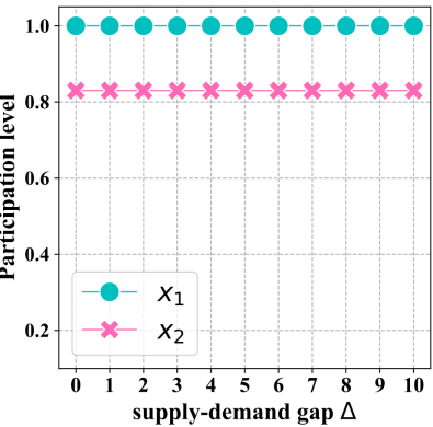
(a) $\Delta-\bm{x}$

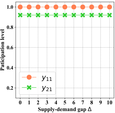
(b) $\Delta-\bm{y}$

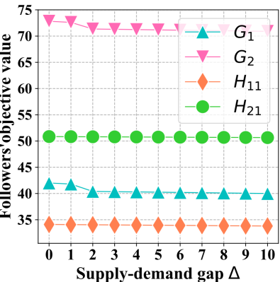
(c) $\Delta-\bm{G}$ and $\Delta-\bm{H}$

For the convenience of analyzing the two-sided MaaS markets, we assume that followers at both sides of the MaaS market are accepted by the leader ($u_{1}=1$, $u_{2}=1$, $w_{11}=1$, $w_{21}=1$). Given the unit threshold price $p=\$1$ and $q=\$2$ for travelers and TSPs, when the value of $\Delta$ is changed from 0 to 10, we solve the corresponding follower problem (T.1)-(T.4) and (P.1)-(P.4) to obtain the values of $x_{1}$, $x_{2}$, $y_{11}$ and $y_{21}$. We analyze the relationship between the supply-demand gap ($\Delta$) and followers’ participation levels/objective values in Figure 3c/Figure 4c. As $\Delta$ increases in SLMFG-L, the participation level of each traveler ($\bm{x}$) and TSP ($\bm{y}$) will not change (Figure 3a and 3b), and each traveler’s objective value ($\bm{G}$) and TSP’s objective value ($\bm{H}$) will slightly decrease (Figure 3c). As $\Delta$ increases in SLMFG-Q, each follower’s participation level ($\bm{x}$ and $\bm{y}$) will increase (Figure 4a and 4b), and each follower’s objective value ($\bm{G}$ and $\bm{H}$) will considerably decrease (Figure 4c).

Figure 4: The relationship between $\Delta$ and followers’ participation level/objective value in SLMFG-Q.

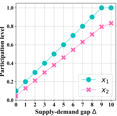
(a) $\Delta-\bm{x}$

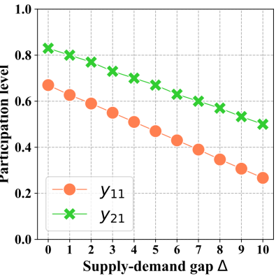
(b) $\Delta-\bm{y}$

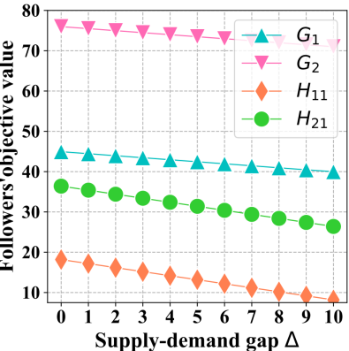
(c) $\Delta-G_{1},\Delta-H_{1}$

Figure 5: The relationship between the unit threshold price $p,q$ and followers’ participation level $\bm{x},\bm{y}$ in SLMFG-L.

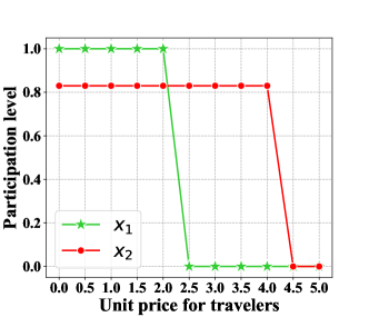
(a) $p-\bm{x}$

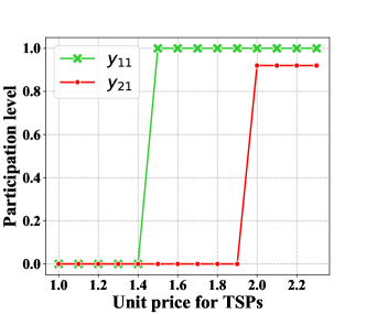
(b) $q-\bm{y}$

Then we analyze the impacts of unit threshold price for travelers and TSPs ($p$ and $q$) determined by the MaaS regulator on their participation levels ($\bm{x}$ and $\bm{y}$). As is shown in Figure 5a, if $p\leq b_{1}\leq b_{2}$, then $x_{1}=1$ and $x_{2}=0.83$; if $b_{1}\leq p\leq b_{2}$, then $x_{1}=0$, $x_{2}=0.83$; and if $b_{1}\leq b_{2}\leq p$, then $x_{1}=0$, $x_{2}=0$. Analogously, as the value of $q$ increases from 1 to 2.2, the value of $w_{11}$ and $u_{21}$ will change, leading to the change of TSPs’ participation levels. In Figure 5b, when $\beta_{11}\leq\beta_{21}\leq q$, $y_{11}=0$, $y_{21}=0$; when $\beta_{11}\leq q\leq\beta_{21}$, $y_{11}=1$, $y_{21}=0$; when $\beta_{11}\leq\beta_{21}\leq q$, $y_{11}=1$, $y_{21}=0.85$.

The results of Example 1 are displayed in Figure 3c-5b. We summarize the obtained insights facilitating the MaaS regulator to manage the platform in two-sided markets.

Observation 1

Based on the above analysis, the reciprocal interactions among the MaaS regulator, travelers and TSPs can be observed in the SLMFG with network effects (SLMFG-Q). As the supply-demand increases, travelers’ participation level will increase and TSPs’ participation level will decrease, and both travelers’ costs and TSPs’ profits will decrease. Moreover, the participation level of travelers (resp. TSPs) are endogenously dependent on the unit threshold price for travelers (resp. TSPs) determined by the MaaS regulator. As the unit threshold price for travelers increases, travelers’ participation levels decrease. Conversely, as the unit threshold price for TSPs increases, TSPs’ participation levels increase.

4 Solution methods

In Section 4.1, we present two approaches to reformulate SLMFG-L and SLMFG-Q based on the optimality conditions of the follower problems: i) KKT conditions and ii) SD conditions. The classic B&B algorithm proposed by Bard and Moore (1990), $\mathsf{Bard\&Moore}$, is based on the MPEC reformulation serving as the benchmark in our numerical experiments. In Section 4.2, we propose a SD-based B&B algorithm to solve both MILBP and MIQBP problems. In Section 4.3, we present a numerical example to illustrate the proposed B&B algorithm.

4.1 Single-level reformulation

MPEC reformulations for SLMFG-L and SLMFG-Q  are introduced in Section 4.1.1 while the SD-based reformulations for both problems are given in Section 4.1.2.

4.1.1 MPEC reformulation.

A classical numerical treatment of bilevel optimization problems is to replace the follower problems by the system of equations/inequations composed of the concatenation of their KKT conditions and then to solve the resulting MPEC. Our aim in this subsection is not only to describe the MPEC formulations associated with the MILBP and MIQBP problems but also to show that, using the specific structure of these problems, it is possible to prove that the bilevel formulations and the corresponding MPEC formulation are equivalent and generate the same solutions (decision variables). This quite rare fact is important to emphasize and will be respectively given in Theorem 4.1 for MILBP problem and Theorem 4.2 for MIQBP problem.

Let us first consider MILBP (SLMFG-L). According to Proposition 3.2, the associated KKT conditions of Traveler $i$’s problem and TSP $mn$’s problem in SLMFG-L are given in Online Appendix 9.1, i.e., Eqs. (KL.1)-(KL.4) and (KL.5)-(KL.8), respectively.

Then the MPEC formulation of SLMFG-L is denoted MPEC-L and summarized in Model 2.1.
Model 2.1 (MPEC-L)

$$\max_{p,q,\bm{l},\bm{u},\bm{w},\Delta,\bm{x},\bm{y},\bm{\lambda},\bm{\mu}}\quad\text{MaaS regulator's profits}\quad\eqref{B1a}$$

subject to:

$$\text{The MaaS regulator's constraints:}\quad\eqref{B1b}-\eqref{B1p},$$

$$\text{Traveler $i$'s KKT conditions:}\quad\eqref{29a}-\eqref{29d},$$

$$\text{TSP $mn$'s KKT conditions:}\quad\eqref{31a}-\eqref{31d},$$

where $\bm{\lambda}$ and $\bm{\mu}$ stand respectively for $\bm{\lambda}=\left(\lambda^{1}_{i},\lambda^{2}_{i},\lambda^{3}_{i}\right)_{i\in\mathcal{I}}$ and $\bm{\mu}=\left(\mu^{1}_{mn},\mu^{2}_{mn},\mu^{3}_{mn}\right)_{\stackrel{{\scriptstyle m\in\mathcal{M}}}{{n\in\mathcal{N}}}}$.

It is well known that usually SLMFG and their associated MPEC reformulations are not equivalent, roughly speaking, they don’t share the same solutions, e.g. Aussel and Svensson (2018, 2019a). As analyzed in Aussel and Svensson (2020), some convexity assumptions coupled with quite strong qualification conditions are needed to guarantee such an equivalence. Nevertheless, SLMFG-L is equivalent to the MPEC reformulation MPEC-Lunder some mild hypothesis. We provide constraint qualifications for SLMFG-L in Theorem 4.1.

Theorem 4.1

Assume that the perceived waiting/idle time functions of travelers/TSPs are linear.

• If $(p,q,\bm{l},\bm{u},\bm{w},\Delta,\bm{x},\bm{y})$ is a global solution of SLMFG-L (or equivalently SLMFG without network effects given in Proposition 3.2), then $\forall(\bm{\lambda},\bm{\mu})\in\Lambda(p,q,\bm{l},\bm{u},\bm{w},\Delta,\bm{x},\bm{y})$, $(p,q,\bm{l},\bm{u},\bm{w},\Delta,\bm{x},\bm{y},\bm{\lambda},\bm{\mu})$ is a global solution of the associated MPEC-L.

• Assume additionally that

  • for all Traveler $i\in\mathcal{I}$, $b_{i}\geq p_{min}$;

  • for all TSP $n\in\mathcal{N}_{m},m\in\mathcal{M}$, $\beta_{mn}\leq q_{max}$.

  If $(p,q,\bm{l},\bm{u},\bm{w},\Delta,\bm{x},\bm{y},\bm{\lambda},\bm{\mu})$ is a global solution of MPEC-L, then $(p,q,\bm{l},\bm{u},\bm{w},\Delta,\bm{x},\bm{y})$ is a global solution of SLMFG-L (or equivalently SLMFG without network effects).

In Theorem 4.1, the set $\Lambda(\cdot)$ denotes the set of Lagrange multipliers associated to the concatenated KKT conditions of the followers (travelers and TSPs). The proof of this theorem is fully described in Online Appendix 10. Let us say thanks to the decoupled structure of the MILBP, to the linearity of the constraints and objective functions of the follower’s problem and finally to the binary character of the leader’s variables $(u_{i})_{i\in\mathcal{I}}$ and $(w_{mn})_{\stackrel{{\scriptstyle m\in\mathcal{M}}}{{n\in\mathcal{N}}}}$, we will be in a position to prove the three main hypothesis of Aussel and Svensson (2020), i.e., the joint convexity of the constraint functions of the followers’ problem, the Joint Slater’s qualification condition and the Guignard’s qualification conditions for boundary opponent strategies (see Proof in Online Appendix 10).

As for SLMFG-Q, The KKT conditions of Traveler $i$’s problem and TSP $mn$’s problem are given in Online Appendix 9.2, i.e., Eqs. (KQ.1)-(KQ.4) and Eqs. (KQ.5)-(KQ.8), respectively. The MPEC formulation associated to SLMFG-Q is denoted as MPEC-Q and summarized in Model 2.2:
Model 2.2 (MPEC-Q)

$$\max_{p,q,\bm{l},\bm{u},\bm{w},\Delta,\bm{x},\bm{y},\bm{\lambda},\bm{\mu}}\quad\text{MaaS regulator's profits}\quad\eqref{B1a}$$

subject to:

$$\text{The MaaS regulator's constraints:}\quad\eqref{B1b}-\eqref{B1p},$$

$$\text{Traveler $i$'s KKT conditions:}\quad\eqref{48a}-\eqref{48d},$$

$$\text{TSP $mn$'s KKT conditions:}\quad\eqref{49a}-\eqref{49d},$$

Mimicking the same arguments as in Theorem 4.1, one can easily establish that, in the case of the quadratic perceived waiting/idle time functions and under some mild hypothesis, SLMFG-Q is equivalent to MPEC-Q. We provide constraint qualifications for SLMFG-Q in Theorem 4.2.

Theorem 4.2

Assume that the perceived waiting/idle time functions of followers are quadratic.

• If $(p,q,\bm{l},\bm{u},\bm{w},\Delta,\bm{x},\bm{y})$ is a global solution of SLMFG-Q (or equivalently MIQBP described in Proposition 3.3) then, for any $(\bm{\lambda},\bm{\mu})\in\Lambda(p,q,\bm{l},\bm{u},\bm{w},\Delta,\bm{x},\bm{y})$, $(p,q,\bm{l},\bm{u},\bm{w},\Delta,\bm{x},\bm{y},\bm{\lambda},\bm{\mu})$ is a global solution of the associated MPEC-Q.

• Assume additionally that

  • for all Traveler $i\in\mathcal{I}$, $b_{i}\geq p_{min}$;

  • for all TSP $n\in\mathcal{N}_{m},m\in\mathcal{M}$, $\beta_{mn}\leq q_{max}$.

  If $(p,q,\bm{l},\bm{u},\bm{w},\Delta,\bm{x},\bm{y},\bm{\lambda},\bm{\mu})$ is a global solution of MPEC-Q, then $(p,q,\bm{l},\bm{u},\bm{w},\Delta,\bm{x},\bm{y})$ is a global solution of SLMFG-Q (or equivalently SLMFG with network effects in Proposition 3.3).

Each of MPEC-L and MPEC-Q contain eight nonlinear constraints (four for traveler’s problems and four for TSP’s problems) corresponding to complementary slackness conditions.

4.1.2 SD-based single-level formulation.

An alternative reformulation consists of replacing the follower problems by their strong-duality (SD) optimality conditions.

The SD conditions of SLMFG-L are given in (DL.1)-(DL.8):

$$\text{Traveler $i$'s constraints}\leavevmode\nobreak\ \eqref{BL1b}-\eqref{BL1d}, \forall i\in\mathcal{I},$$ (DL.1)

$$(r_{i}-b_{i})Q_{i}x_{i}\geq B_{i}\bar{\lambda}_{1}^{i}+u_{i}\bar{\lambda}_{2}^{i}, \forall i\in\mathcal{I},$$ (DL.2)

$$b_{i}Q_{i}\bar{\lambda}_{1}^{i}+\bar{\lambda}_{2}^{i}\geq(r_{i}-b_{i})Q_{i}, \forall i\in\mathcal{I},$$ (DL.3)

$$\bar{\lambda}_{1}^{i},\bar{\lambda}_{2}^{i}\geq 0, \forall i\in\mathcal{I},$$ (DL.4)

$$\text{TSP $mn$'s constraints}\leavevmode\nobreak\ \eqref{BL2b}-\eqref{BL2d}, \forall m\in\mathcal{M},n\in\mathcal{N}_{m},$$ (DL.5)

$$(\beta_{mn}-\rho_{mn})C_{mn}y_{mn}\geq\bar{B}_{mn}\bar{\mu}_{1}^{mn}+w_{mn}\bar{\mu}_{2}^{mn}, \forall m\in\mathcal{M},n\in\mathcal{N}_{m},$$ (DL.6)

$$C_{mn}\gamma_{mn}\bar{\mu}_{1}^{mn}+\bar{\mu}_{2}^{mn}\geq(\beta_{mn}-\rho_{mn})C_{mn}, \forall m\in\mathcal{M},n\in\mathcal{N}_{m},$$ (DL.7)

$$\bar{\mu}_{1}^{mn},\bar{\mu}_{2}^{mn}\geq 0, \forall m\in\mathcal{M},n\in\mathcal{N}_{m},$$ (DL.8)

where $\bar{\lambda}_{1}^{i},\bar{\lambda}_{2}^{i}$ denotes the dual variables corresponding to the primal constraint (T.2) and (T.3), respectively. $\bar{\mu}_{1}^{mn},\bar{\mu}_{2}^{mn}$ denotes the dual variables corresponding to primal constraint (P.2) and (P.3), respectively. (DL.2) compares the objective value of Traveler $i$’s primal problem on the left hand side with that of its dual problem on the right hand side, (DL.3) is the dual constraint of Traveler $i$; (DL.6) compares the objective value of the TSP $mn$’s primal problem on the left hand side with its dual problem on the right hand side and (DL.7) is the dual constraint of TSP $mn$. The resulting SD reformulation of SLMFG-L is denoted by SD-L and is summarized in Model 3.1.

Model 3.1 (SD-L)

$$F=\max_{p,q,\bm{l},\bm{u},\bm{w},\Delta,\bm{x},\bm{y},\bm{\bar{\lambda}},\bm{\bar{\mu}},}\quad\text{MaaS regulator's profits}\quad\eqref{B1a}$$

subject to

$$\text{MaaS regulator's constraints}\quad\eqref{B1b}-\eqref{B1p},$$

$$\text{Traveler $i$'s duality conditions}\quad\text{\eqref{DU2aa}-\eqref{DU2c}},$$

$$\text{TSP $mn$'s duality conditions}\quad\text{\eqref{DU2dd}-\eqref{DU2f}}.$$

It is well-known that, for linear bilevel optimization problems, single-level reformulations based on SD conditions are equivalent to single-level reformulations based on KKT conditions (Fortuny-Amat and McCarl 1981, Zare et al. 2019, Kleinert et al. 2020b). Hence, a direct extension of Theorem 4.1 is that, assuming the same conditions as stated therein, the solutions of SD-L are also solutions of SLMFG-L and reciprocally. This result is summarized in Corollary 11.1 in Online Appendix 11.1.

We next derive the SD reformulation of SLMFG-Q, which is more technical since follower problems therein are strictly convex quadratic (as opposed to linear in SLMFG-L). We give primal-dual formulations of SLMFG-Q in Lemma 11.2 in Online Appendix 11.2.

Based on Lemma 11.2, SD conditions of SLMFG-Q are summarized in Eqs.(DQ.1)-(DQ.6).

$$\text{Traveler $i$'s constraints}\leavevmode\nobreak\ \eqref{BL1b}-\eqref{BL1d},\forall i\in\mathcal{I},$$ (DQ.1)

$$\frac{\zeta\alpha_{i}Q_{i}^{2}}{C^{2}}x_{i}^{2}-\left(\frac{2\zeta\alpha_{i}Q_{i}}{\bar{C}}-\frac{2\zeta\alpha_{i}\Delta}{C^{2}}+r_{i}-b_{i}\right)Q_{i}x_{i}\leq-\frac{(A_{i}\bar{\lambda}_{1}^{i})^{2}+(\bar{\lambda}_{2}^{i})^{2}}{2P_{i}}-\frac{U_{i}}{P_{i}}\left(b_{i}Q_{i}\bar{\lambda}_{1}^{i}+\bar{\lambda}_{2}^{i}\right)$$

$$-\frac{b_{i}Q_{i}\bar{\lambda}_{1}^{i}\bar{\lambda}_{2}^{i}}{P_{i}}-\frac{U_{i}^{2}}{2P_{i}}-B_{i}\bar{\lambda}_{1}^{i}-\bar{\lambda}_{2}^{i}u_{i},\forall i\in\mathcal{I},$$ (DQ.2)

$$\bar{\lambda}_{1}^{i},\bar{\lambda}_{2}^{i}\geq 0,\forall i\in\mathcal{I},$$ (DQ.3)

$$\text{TSP $mn$'s constraints}\leavevmode\nobreak\ \eqref{BL2b}-\eqref{BL2d},\forall m\in\mathcal{M},n\in\mathcal{N}_{m},$$ (DQ.4)

$$\frac{\kappa\eta_{mn}C_{mn}^{2}}{C^{2}}y_{mn}^{2}-\left(\frac{2\kappa\eta_{mn}\Delta}{C^{2}}+\beta_{mn}-\rho_{mn}\right)C_{mn}y_{mn}\leq-\frac{(A_{mn}\bar{\mu}_{1}^{mn})^{2}+(\bar{\mu}_{2}^{mn})^{2}}{2P_{mn}}$$

$$-\frac{U_{mn}}{P_{mn}}\left(A_{mn}\bar{\mu}_{1}^{mn}+\bar{\mu}_{2}^{mn}\right)-\frac{A_{mn}\bar{\mu}_{1}^{mn}\bar{\mu}_{2}^{mn}}{P_{mn}}-\frac{U_{mn}^{2}}{2P_{mn}}-\bar{B}_{mn}\bar{\mu}_{1}^{mn}-w_{mn}\bar{\mu}_{2}^{mn},\forall m\in\mathcal{M},n\in\mathcal{N}_{m},$$ (DQ.5)

$$\bar{\mu}_{1}^{mn},\bar{\mu}_{2}^{mn}\geq 0,\forall m\in\mathcal{M},n\in\mathcal{N}_{m},$$ (DQ.6)

where (DQ.2) compares the objective value of Traveler $i$’s primal problem on the left hand side with that of Traveler $i$’s dual follower problem on the right hand side, and (DQ.5) compares the objective value of TSP $mn$’s primal problem on the left hand side with that of TSP $mn$’s dual follower problem on the right hand side.

Unlike the SD conditions of the follower problems of SLMFG-L, SD conditions of the follower problems of SLMFG-Q involve bilinear terms which are product of continuous variables, namely, $\Delta\cdot x_{i}$ and $\Delta\cdot y_{mn}$ in (DQ.2) and (DQ.5), respectively. We relax these bilinear terms by introducing auxiliary variables $W_{i}\triangleq\Delta\cdot x_{i}$ and $W_{mn}\triangleq\Delta\cdot y_{mn}$ using their McCormick envelopes (McCormick 1976). Accordingly, constraints (MK.1)-(MK.8) are added to the SD reformulation of SLMFG-Q.

The SD-based reformulation of SLMFG-Q is denoted SD-Q and summarized in Model 3.2.
Model 3.2 (SD-Q)

$$\max_{p,q,\bm{l},\bm{u},\bm{w},\Delta,\bm{x},\bm{y},\bm{\bar{\lambda}},\bm{\bar{\mu}}}\quad\text{MaaS regulator's profits}\quad\eqref{B1a},$$

subject to

$$\text{MaaS regulator's constraints}\quad\text{\eqref{B1b}-\eqref{B1p}},$$

$$\text{Traveler $i$'s duality conditions }\quad\eqref{DUa}-\eqref{DUc},\eqref{MKa}-\eqref{MKd},$$

$$\text{TSPs' duality conditions }\quad\eqref{DUd}-\eqref{DUf},\eqref{MKe}-\eqref{MKh}.$$

Since the duality gap for convex optimization problems is null, SD conditions are equivalent to KKT conditions, Hence, analogously to Corollary 11.1, a direct extension of Theorem 4.2 is given in Corollary 11.4 in Online Appendix 11.3.

Observe that SD-Q is a relaxation of SLMFG-Q whereas SD-L is an exact reformulation of SLMFG-L. We next present the customized B&B algorithms based on formulations SD-L and SD-Q to solve SLMFG-L and SLMFG-Q, respectively.

4.2 SD-based B&B algorithm

In SD-L and SD-Q, the nonlinear terms $\bar{\lambda}_{2}^{i}u_{i}$ in (DL.2) and (DQ.2), and $\bar{\mu}_{2}^{mn}w_{mn}$ in (DL.6) and (DQ.5) could be linearized using classic big-$M$ approaches, however, finding valid big-$M$ values is non-trivial (Kleinert et al. 2020a). To circumvent this difficulty , we propose a customized B&B algorithm, $\mathsf{SD}$-$\mathsf{B\&B}$, which branches on the binary variables $u_{i}$ and $w_{mn}$.

In SD-L, $\mathsf{SD}$-$\mathsf{B\&B}$ algorithm starts by relaxing all nonlinear constraints (DL.2) and (DL.6). This relaxed problem is thus a MILBP which ignores the optimality conditions of followers. This relaxation is also known as the High-Point-Relaxation (HPR). Upon solving the HPR, the optimality conditions of followers are examined and a sub-optimal follower is selected (otherwise the solution is bilevel-optimal). If the sub-optimal follower represents a traveler $i^{\prime}\in\mathcal{I}$, two children nodes are generated with the constraints $u_{i^{\prime}}=0$ and $u_{i^{\prime}}=1$, respectively, and the corresponding constraint (DL.2) is added to both children nodes. Otherwise, the sub-optimal follower must represent a TSP $mn^{\prime}\in\mathcal{MN}$ and two children nodes are generated with the constraints $w_{mn^{\prime}}=0$ and $w_{mn^{\prime}}=1$, respectively, and the corresponding constraint (DL.6) is added to both children nodes. Observe that the added constraints (DL.2) and (DL.6) in the generated children nodes are linear since the binary variables therein are fixed. Analogically, in SD-Q, $\mathsf{SD}$-$\mathsf{B\&B}$ algorithm starts by solving the HPR problem, which is a MIQBP. If the sub-optimal follower represents a traveler $i^{\prime}\in\mathcal{I}$, two children nodes are generated and the corresponding constraint (DQ.2) together with its McCormick envelopes (MK.1)-(MK.4) are added to both children nodes. Otherwise, the sub-optimal follower must represent a TSP $mn^{\prime}\in\mathcal{MN}$, two children nodes are generated and the corresponding constraint (DQ.5) together with its McCormick envelopes (MK.5)-(MK.8) are added to both children nodes. Observe that the nonlinear terms $\bar{\lambda}_{2}^{i}u_{i}$ and $\bar{\mu}_{2}^{mn}w_{mn}$ of the constraints added in the generated children nodes are linearized since the binary variables are therein fixed.

We next introduce some formal notations to present the proposed $\mathsf{SD}$-$\mathsf{B\&B}$ algorithm.

4.2.1 Follower optimality.

Let $\overline{\mathcal{I}}_{0}=\left\{i\in\mathcal{I}:u_{i}=0\right\}$ and $\overline{\mathcal{I}}_{1}=\left\{i\in\mathcal{I}:u_{i}=1\right\}$ be the sets of accepted and rejected travelers, respectively. These sets are initialized to be empty sets at the root node of the B&B tree. The set of undecided travelers is $\widehat{\mathcal{I}}=\mathcal{I}\setminus\{\mathcal{I}_{0}\cup\mathcal{I}_{1}\}$. Analogously, we define the sets of accepted/rejected TSPs as $\overline{\mathcal{MN}}_{0}=\left\{(m,n)\in\mathcal{MN}:w_{mn}=0\right\}$ and $\overline{\mathcal{MN}}_{1}=\left\{(m,n)\in\mathcal{MN}:w_{mn}=1\right\}$, respectively; and the set of undecided TSPs as $\widehat{\mathcal{MN}}=\mathcal{MN}\setminus\{\overline{\mathcal{MN}}_{0}\cup\overline{\mathcal{MN}}_{1}\}$.

To check the optimality of follower problems, we solve a series of single-variable linear programs (one per follower) parameterized by the leader solution $(\bm{u},\bm{w},\Delta)$. Specifically, at any node of the B&B tree, for all travelers $i\in\widehat{\mathcal{I}}$, we solve (T.1)-(T.4) and compare the obtained objective value $G_{i}^{*}$ (optimal response) with the evaluation of (T.1), denoted $\hat{G}_{i}$, based on the relaxed solution obtained at this node. If $|G_{i}^{*}-\hat{G}_{i}|>\epsilon$, for a tolerance $\epsilon$, e.g., $\epsilon=1\times 10^{-4}$, then traveler $i$ is considered sub-optimal and added to the set $\mathcal{V}_{travel}$ of sub-optimal travelers. The same process is implemented for TSPs. The pseudocode of is summarized in Algorithm 1.

Input: $\Delta,\bm{u},\bm{w}$

Output: $\mathcal{V}_{travel},\mathcal{V}_{TSP},O_{i},O_{mn}$

1 for $i\in\mathcal{I}$  do

2       $G_{i}^{*}\leftarrow$ solve Traveler $i$’s follower problem (T.1)-(T.4), given $u_{i},\Delta$

3       $\hat{G}_{i}\leftarrow$ substitute $x_{i}$ and $\Delta$ into Traveler $i$’s objective function (T.1)

4       $O_{i}\leftarrow|G_{i}^{*}-\hat{G}_{i}|$

5       if $|G_{i}^{*}-\hat{G}_{i}|>\epsilon$ then

6            $\mathcal{V}_{travel}\leftarrow\mathcal{V}_{travel}\cup\left\{i\right\}$

7for (m,n) in $\mathcal{MN}$  do

8       $H_{mn}^{*}\leftarrow$ solve TSP $mn$’s follower problem (P.1)-(P.4), given $w_{mn},\Delta$

9       $\hat{H}_{mn}\leftarrow$ substitute $y_{mn}$ into TSP $mn$’s objective function (P.1)

10       $O_{mn}\leftarrow|H_{mn}^{*}-\hat{H}_{mn}|$

11       if $|H_{mn}^{*}-\hat{H}_{mn}|>\epsilon$ then

12            $\mathcal{V}_{TSP}\leftarrow\mathcal{V}_{TSP}\cup\left\{(m,n)\right\}$

Algorithm 1 Updating the non-optimal sets of followers

4.2.2 Branching rules.

We first branch on TSPs accept/reject variables $\bm{w}$ before branching on travelers accept/reject variables $\bm{u}$. This is motivated by empirical evidence and the fact that in realistic instances the number of TSPs is expected to be substantially smaller than the number of travelers. We customize three types of branching rules to select the branching variable among suboptimal followers:
1) $\mathsf{SD}$-$\mathsf{BP}$: If $\widehat{\mathcal{MN}}\neq\varnothing$, select a branching variable $w_{mn}$ corresponding to TSP $mn$ with the minimum sell-bidding price $\beta_{mn}$, $\forall(m,n)\in\mathcal{V}_{TSP}$. Otherwise, if $\widehat{\mathcal{I}}\neq\varnothing$, select a branching variable $u_{i}$ corresponding to Traveler $i$ with the maximum purchase-bidding price $b_{i}$, $\forall i\in\mathcal{V}_{travel}$.

2) $\mathsf{SD}$-$\mathsf{Diffob}$: If $\widehat{\mathcal{MN}}\neq\varnothing$, select a branching variable $w_{mn}$ corresponding to TSP $mn$ with the maximum optimality gap $|H_{mn}^{*}-\hat{H}_{mn}|$, $\forall(m,n)\in\mathcal{V}_{TSP}$. Otherwise, if $\widehat{\mathcal{I}}\neq\varnothing$, select a branching variable $u_{i}$ corresponding to Traveler $i$ with the maximum optimality gap $|G_{i}^{*}-\hat{G}_{i}|,\forall i\in\mathcal{V}_{travel}$.

3) $\mathsf{SD}$-$\mathsf{Wi}$: combine the above two rules by introducing a weighting factor $\theta$. If $\widehat{\mathcal{MN}}\neq\varnothing$, select a branching variable corresponding to TSP $mn$ with the maximum weighted value $\theta|H_{mn}^{*}-\hat{H}_{mn}|+(1-\theta)\beta_{mn}$. Otherwise, if $\widehat{\mathcal{I}}\neq\varnothing$, select a branching variable corresponding to Traveler $i$ with the maximum weighted value $\theta|G_{i}^{*}-\hat{G}_{i}|+(1-\theta)b_{i}$.

The pseudocode of the branching rules is summarized in Algorithm 2.

Input: $\widehat{\mathcal{MN}},\widehat{\mathcal{I}},\mathcal{V}_{travel},\mathcal{V}_{TSP},b_{i},\beta_{mn},O_{i},O_{mn}$

Output: $\overline{\mathcal{I}}_{0}$, $\overline{\mathcal{I}}_{1},\overline{\mathcal{MN}}_{0},\overline{\mathcal{MN}}_{1},\mathcal{L}$

1 if $\widehat{\mathcal{MN}}\neq\varnothing$ then

2       if branching rule is $\mathsf{SD}$-$\mathsf{BP}$ then

3             $(m,n)\leftarrow argmin_{(m,n)\in\mathcal{V}_{TSP}}\left\{\beta_{mn}\right\}$ $\triangleright$ COMMENTselect $(m,n)$ of $\mathcal{V}_{TSP}$ with minimum bidding price

4      if branching rule is $\mathsf{SD}$-$\mathsf{Diffob}$ then

5             $(m,n)\leftarrow argmax_{(m,n)\in\mathcal{V}_{TSP}}\left\{O_{mn}\right\}$ $\triangleright$ COMMENTselect $(m,n)$ of $\mathcal{V}_{TSP}$ with maximum optimality gap

6      if branching rule is $\mathsf{SD}$-$\mathsf{Wi}$ then

7             $Z_{mn}\leftarrow\theta\cdot O_{mn}+(1-\theta)\cdot\beta_{mn}$

8             $(m,n)\leftarrow argmax_{(m,n)\in\mathcal{V}_{TSP}}\left\{Z_{mn}\right\}$ $\triangleright$ COMMENTselect $(m,n)$ of $\mathcal{V}_{TSP}$ with maximum weighted value

9       $s_{2}\leftarrow(m,n)$

10       $\overline{\mathcal{MN}}_{0}\leftarrow\overline{\mathcal{MN}}_{0}\cup\{s_{2}\}$ $\triangleright$ COMMENTadd the new branching index to the fixed set $\overline{\mathcal{MN}}_{0}$

11       $\overline{\mathcal{MN}}_{1}\leftarrow\overline{\mathcal{MN}}_{1}\cup\{s_{2}\}$ $\triangleright$ COMMENTadd the new branching index to the fixed set $\overline{\mathcal{MN}}_{1}$

12       $n\leftarrow\text{len}(\mathcal{L})$ $\triangleright$ COMMENTupdate the left child node

13       $\mathcal{L}\leftarrow\mathcal{L}\cup\{n\}$ $\triangleright$ COMMENTupdate the set of active nodes

14      

15else if $\widehat{\mathcal{I}}\neq\varnothing$ then

16      if branching rule is $\mathsf{SD}$-$\mathsf{BP}$ then

17             $i\leftarrow argmax_{i\in\mathcal{V}_{travel}}\left\{b_{i}\right\}$ $\triangleright$ COMMENTselect $i$ of $\mathcal{V}_{travel}$ with the maximum bidding price

18      if branching rule is $\mathsf{SD}$-$\mathsf{Diffob}$ then

19             $i\leftarrow argmax_{i\in\mathcal{V}_{travel}}\left\{O_{i}\right\}$ $\triangleright$ COMMENTselect $i$ of $\mathcal{V}_{travel}$ with the maximum optimality gap

20      if branching rule is $\mathsf{SD}$-$\mathsf{Wi}$ then

21             $Z_{i}\leftarrow\theta\cdot O_{i}+(1-\theta)\cdot b_{i}$

22             $i\leftarrow argmax_{i\in\mathcal{V}_{travel}}\left\{Z_{i}\right\}$ $\triangleright$ COMMENTselect $i$ of $\mathcal{V}_{travel}$ with the maximum weighted value

23      $s_{1}\leftarrow i$

24       $\overline{\mathcal{I}}_{0}\leftarrow\overline{\mathcal{I}}_{0}\cup\{s_{1}\}$ $\triangleright$ COMMENTadd new branching index to the fixed set $\overline{\mathcal{I}}_{0}$

25       $\overline{\mathcal{I}}_{1}\leftarrow\overline{\mathcal{I}}_{1}\cup\{s_{1}\}$ $\triangleright$ COMMENTadd new branching index to the fixed set $\overline{\mathcal{I}}_{1}$

26       $n\leftarrow n+1$ $\triangleright$ COMMENTupdate the right child node

27       $\mathcal{L}\leftarrow\mathcal{L}\cup\{n\}$ $\triangleright$ COMMENTupdate the set of active nodes

28      

Algorithm 2 Branching procedure

4.2.3 Algorithm summary.

The proposed $\mathsf{SD}$-$\mathsf{B\&B}$ algorithm is summarized in Algorithm 3. SP denotes a sub-problem at a node of the B&B tree and index $k$ is a superscript to track the current B&B node in the while loop, the formulations of the sub-problem $\textit{SP}^{k}$ of SLMFG-L and SLMFG-Q are provided in Online Appendix 12. The list of active sub-problem indices is denoted $\mathcal{L}$ and initialized with the root node sub-problem, i.e. the HPR of the SD-L or SD-Q. UB and LB are used to track upper and lower bounds throughout the process.

Input: $\mathcal{B}_{i},\mathcal{B}_{mn}$

Output: $k,\overline{\textit{UB}},LB,Gap$

1 $Gap\leftarrow\infty$, $\text{LB}\leftarrow-\infty$, $n\leftarrow 0$ $\mathcal{L}\leftarrow\left\{n\right\}$ $\triangleright$ COMMENTinitialization

2 $\overline{\mathcal{I}}_{0}^{k}\leftarrow\left\{\right\}$, $\overline{\mathcal{I}}_{1}^{k}\leftarrow\left\{\right\},\overline{\mathcal{MN}}_{0}^{k}\leftarrow\left\{\right\},\overline{\mathcal{MN}}_{1}^{k}\leftarrow\left\{\right\}$ $\triangleright$ COMMENTinitialize the fixed sets

3 $\textit{SP}^{0}\leftarrow\text{HPR}\left(\mathcal{B}_{i},\mathcal{B}_{mn}\right)$, $\triangleright$ COMMENTsolve high-point-relaxation problem

4 $\overline{\textit{UB}}\leftarrow F^{0}(p^{0},q^{0},\bm{l}^{0},\bm{u}^{0},\bm{w}^{0},\Delta^{0},\bm{x}^{0},\bm{y}^{0})$ $\triangleright$ COMMENTthe objective value of HPR

5 $k\leftarrow 1$

6 while $\mathcal{L}\neq\varnothing$  do

7       parent node $\leftarrow$ select a node from $\mathcal{L}$ $\triangleright$ COMMENTbest bound first search

8       $F^{k}$ $\leftarrow\textit{SP}^{k}$ $\left(\mathcal{B}_{i},\mathcal{B}_{mn},\textit{SP}^{k-1},\overline{\mathcal{I}}_{0}^{k},\overline{\mathcal{I}}_{1}^{k},\overline{\mathcal{MN}}_{0}^{k},\overline{\mathcal{MN}}_{1}^{k}\right)$ $\triangleright$ COMMENTsolve the $kth$ sub-problem

9       if $\textit{SP}^{k}$ is infeasible then

10             $\textit{UB}^{k}\leftarrow F^{k}(p^{k},q^{k},\bm{l}^{k},\bm{u}^{k},\bm{w}^{k},\Delta^{k},\bm{x}^{k},\bm{y}^{k})$ $\triangleright$ COMMENTobtain UB

11             $\mathcal{V}_{travel}^{k},\mathcal{V}_{TSP}^{k},O_{i}^{k},O_{mn}^{k}\leftarrow\textbf{{\color[rgb]{0,0,0}Algorithm} }\ref{alg1}$ $(\Delta^{k},\bm{u}^{k},\bm{w}^{k})$

12             if all the followers are optimal ($\mathcal{V}_{travel}^{k}=\varnothing,\mathcal{V}_{TSP}^{k}=\varnothing$) then

13                   if $\textit{UB}^{k}>\textit{LB}$ then

14                         $\textit{LB}\leftarrow\textit{UB}^{k}$ $\triangleright$ COMMENTupdate LB

15                         prune the nodes of $\mathcal{L}$ with $\textit{UB}\leq\textit{LB}$ $\triangleright$ COMMENTfathoming

16             else

17                   $\overline{\mathcal{I}}_{0}^{k}$, $\overline{\mathcal{I}}_{1}^{k},\overline{\mathcal{MN}}_{0}^{k},\overline{\mathcal{MN}}_{1}^{k},\mathcal{L}\leftarrow$ Algorithm 2 ($\widehat{\mathcal{MN}}^{k},\widehat{\mathcal{I}}^{k},\mathcal{V}_{TSP}^{k}$,$\mathcal{V}_{travel}^{k},b_{i},\beta_{mn},O_{i}^{k},O_{mn}^{k}$)

18                  

19      

20       $\mathcal{L}\leftarrow\mathcal{L}-\left\{\textit{parent node}\right\}$, $\triangleright$ COMMENTdelete the selected node from $\mathcal{L}$

21       if $\mathcal{L}=\varnothing$ then

22            $\overline{\textit{UB}}\leftarrow LB$

23             $Gap\leftarrow 0$ $\triangleright$ COMMENTconverged

24      else

25            $\overline{\textit{UB}}\leftarrow$ select an active node of $\mathcal{L}$ with the maximum UB

26             if ($\overline{\textit{UB}}-\textit{LB})/\textit{LB}<Gap$ then

27                  $Gap=(\overline{\textit{UB}}-\textit{LB})/\textit{LB}$ $\triangleright$ COMMENTupdate the gap

28      if $Gap<1\times e^{-6}$ then

29            break $\triangleright$ COMMENTexit by gap

30      $k\leftarrow k+1$

Algorithm 3 SD-based Branch and bound algorithm ($\mathsf{SD}$-$\mathsf{B\&B}$)

4.3 Illustration of Algorithm SD-B&B

We illustrate Algorithm $\mathsf{SD}$-$\mathsf{B\&B}$ using the same data as in Example 1, we consider the linear case, i.e. SLMFG-L (MILBP) and solve it using $\mathsf{SD}$-$\mathsf{B\&B}$ and branching rule $\mathsf{SD}$-$\mathsf{BP}$. The corresponding B&B tree is shown in Figure 6, and the formulation of the $kth$ sub-problem $\textit{SP}^{k}$ of SLMFG-L is provided in Online Appendix 12. At each iteration, the check is made to see if each user and each TSP is in an optimal condition, namely, $\mathcal{V}_{travel}=\varnothing$ and $\mathcal{V}_{TSP}=\varnothing$.

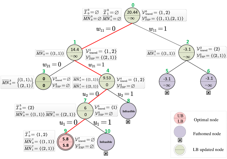
Figure 6: Search tree for the example. The node expansion order is $\bm{0\rightarrow 1\rightarrow 2\rightarrow 3\rightarrow 4\rightarrow 7\rightarrow 8\rightarrow 9\rightarrow 10}.$

At the root node, we solve the HPR problem to obtain $\bm{u}^{0}=(1,1)$, $\bm{w}^{0}=(1,1)$, $\bm{x}^{0}=(1,0.68)$, $\bm{y}^{0}=(0.34,0.32)$ and an objective value $F^{0}=20.44$. Since no follower is optimal, the accept/reject binary variable corresponding to the TSP with the minimum sell-bid is selected as the branching variable, i.e. $w_{11}$ and two children nodes are generated accordingly. Solving sub-problems $SP^{1}$ and $SP^{2}$ yields $F^{1}=14.4$ and $F^{2}=-3.1$, respectively. Follower-optimality is not satisfied, hence both sub-problems generate two children nodes by branching on the other TSP accept/reject variable, i.e. $w_{21}$. Solving $\textit{SP}^{3}$ yields $F^{3}=0$ and all followers are optimal, i.e. $\mathcal{V}_{travel}^{3}=\mathcal{V}_{TSP}^{3}=\varnothing$. Hence, LB is updated to 0 and since $LB>F^{2}$, the children nodes of node 2 (nodes 5 and node 6) are pruned. Solving $\textit{SP}^{4}$ yields $F^{4}=9.53$, but travelers’ problems are sub-optimal, hence the accept/reject variable of the traveler with the maximum purchase-bid, $u_{2}$, is selected for branching. Solving $\textit{SP}^{5}$ at node 7 yields $F^{5}=6$ and since the last undecided traveler is sub-optimal, two children nodes are generated by branching on $u_{1}$. The sub-problem at node 8 is infeasible, thus this node is fathomed. Solving $\textit{SP}^{7}$ at node 9 yields $F^{7}=5.8$ which improves on the current incumbent and thus LB is updated to 5.8. The sub-problem at node 10 is infeasible, thus this node is fathomed and the optimal solution is that corresponding to node 9.

5 Computational study

In this section, we conduct a series of numerical experiments to evaluate the performance of the proposed SLMFG models and $\mathsf{SD}$-$\mathsf{B\&B}$ algorithm. The input data is introduced in Online Appendix 13.1. We examine the impact of followers’ bidding price and the capacity of mobility resources on the SLMFG models. We compare the computational performance of $\mathsf{SD}$-$\mathsf{B\&B}$ algorithm using the three proposed branching rules against a benchmark. The benchmark is the B&B algorithm proposed by Bard and Moore (1990) that branches on complementary slackness conditions of the MPEC reformulation, hereby referred to as $\mathsf{Bard\&Moore}$. All numerical experiments are conducted using Python 3.7.4 and CPLEX Python API on a Windows 10 machine with Intel(R) Core i7-8700 CPU $@$ 3.20 GHz, 3.19 GHz, 6 Core(s) and with 64 GB of RAM.

5.1 Algorithms benchmarking

In this section, we present numerical results of the proposed $\mathsf{SD}$-$\mathsf{B\&B}$ algorithm under three types of branching rules and compare its performance against the benchmark, i.e. Algorithm $\mathsf{Bard\&Moore}$. We implement Algorithm $\mathsf{SD}$-$\mathsf{B\&B}$ using the three proposed branching rule described in Section 4.2.2 and named accordingly: $\mathsf{SD}$-$\mathsf{BP}$, $\mathsf{SD}$-$\mathsf{Diffob}$ and $\mathsf{SD}$-$\mathsf{Wi}$. We consider 20 instances for each group, hence a total of 400 instances are respectively solved for the linear (SLMFG-L) and quadratic (SLMFG-Q) cases using all four methods (three variants of $\mathsf{SD}$-$\mathsf{B\&B}$ and $\mathsf{Bard\&Moore}$), here we only report detailed results of the first three instances of each group of instances for each method. The numerical results for SLMFG-L and SLMFG-Q are summarized in Table 1 and Table 2, respectively, in which each row represents an instance. For each method, the results are organized in four columns: $k$ is the number of sub-problems solved, LB is the objective value of the best integer solution found, Gap is the optimality gap in percentage and $T$ is the total CPU runtime in seconds. We use a time limit of 10800 seconds (3 hours).

Table 1: Performance of the proposed B&B algorithms benchmarked with $\mathsf{Bard\&Moore}$ for SLMFG-L(MILBP)

Instances		$\mathsf{Bard\&Moore}$				$\mathsf{SD}$-$\mathsf{BP}$				$\mathsf{SD}$-$\mathsf{Diffob}$				$\mathsf{SD}$-$\mathsf{Wi}$
		k	LB	Gap(%)	$T(s)$	k	LB	Gap(%)	$T(s)$	k	LB	Gap(%)	$T(s)$	k	LB	Gap(%)	$T(s)$
MaaS-10-5	1	52	19	0	13	32	19	0	8	26	19	0	7	26	19	0	6
	2	63	0	0	15	34	0	0	9	26	0	0	7	26	0	0	6
	3	47	0	0	12	40	0	0	10	28	0	0	7	28	0	0	7
MaaS-30-5	1	76	310	0	24	33	310	0	14	37	310	0	22	25	310	0	11
	2	92	315	0	28	39	315	0	17	46	315	0	23	33	315	0	13
	3	88	314	<$1e^{-6}$	27	41	314	0	16	43	314	0	23	37	314	0	14
MaaS-50-5	1	312	127	0	128	137	127	0	65	155	127	<$1e^{-6}$	86	135	127	<$1e^{-6}$	67
	2	340	243	0	136	136	243	0	70	216	243	<$1e^{-6}$	115	145	243	<$1e^{-6}$	72
	3	236	578	<$1e^{-6}$	108	58	578	0	30	235	578	<$1e^{-6}$	106	88	578	<$1e^{-6}$	40
MaaS-70-6	1	11456	499	0	6823	262	499	0	202	3890	499	0	4569	268	499	0	221
	2	11668	743	0	7021	78	743	0	59	3011	743	0	3895	89	743	0	68
	3	11255	603	0	6802	133	603	<$1e^{-6}$	108	2400	603	0	2890	160	603	0	146
MaaS-90-6	1	18128	-$\infty$	100%	10800	210	832	0	222	595	832	0	10800	595	832	0	611
	2	16887	-$\infty$	100%	10800	217	890	0	242	2281	890	0	10800	2281	890	0	2172
	3	17473	-$\infty$	100%	10800	294	999	<$1e^{-6}$	311	636	999	0	10800	636	999	<$1e^{-6}$	682
MaaS-110-7	1	15436	-$\infty$	100%	10800	234	716	0	226	3777	-$\infty$	100%	10800	1077	716	<$1e^{-6}$	1314
	2	15992	-$\infty$	100%	10800	329	1212	0	379	3677	-$\infty$	100%	10800	967	1212	<$1e^{-6}$	1228
	3	15425	-$\infty$	100%	10800	276	1102	0	298	3985	-$\infty$	100%	10800	1245	1102	<$1e^{-6}$	1442
MaaS-130-7	1	13582	-$\infty$	100%	10800	1030	1034	<$1e^{-6}$	1704	3523	-$\infty$	100%	10800	1432	1034	<$1e^{-6}$	2255
	2	13559	-$\infty$	100%	10800	1342	989	0	2247	3913	-$\infty$	100%	10800	1556	989	0	2378
	3	13902	-$\infty$	100%	10800	1021	1120	0	1689	3803	-$\infty$	100%	10800	1641	1120	0	2417
MaaS-170-9	1	5776	-$\infty$	100%	10800	1516	1671	<$1e^{-6}$	3063	3026	-$\infty$	100%	10800	3869	1671	<$1e^{-6}$	7118
	2	5694	-$\infty$	100%	10800	858	1744	0	1688	2937	-$\infty$	100%	10800	2614	1744	0	4174
	3	5761	-$\infty$	100%	10800	602	1648	0	1224	3141	-$\infty$	100%	10800	834	1648	0	1516
MaaS-190-10	1	4786	-$\infty$	100%	10800	438	1784	0	1028	2240	-$\infty$	100%	10800	3917	1784	<$1e^{-6}$	9800
	2	4955	-$\infty$	100%	10800	519	1702	0	1141	2421	-$\infty$	100%	10800	2233	1702	<$1e^{-6}$	3882
	3	4862	-$\infty$	100%	10800	560	1787	0	1325	2322	-$\infty$	100%	10800	1641	1787	<$1e^{-6}$	3186
MaaS-200-10	1	4632	-$\infty$	100%	10800	1351	1660	0	3155	2230	-$\infty$	100%	10800	2743	1660	<$1e^{-6}$	9116
	2	4616	-$\infty$	100%	10800	2894	1643	0	7572	2688	-$\infty$	100%	10800	3656	1643	<$1e^{-6}$	10262
	3	4457	-$\infty$	100%	10800	877	1847	0	2212	2867	-$\infty$	100%	10800	3923	1847	<$1e^{-6}$	10703

Numbers in bold denotes the smallest CPU runtime for each instance

Table 2: Performance of the proposed B&B algorithms benchmarked with $\mathsf{Bard\&Moore}$ for SLMFG-Q (MIQBP)

Instances		Bard&Moore				SD-BP				SD-Diffob				SD-Wi
		k	LB	Gap(%)	$T(s)$	k	LB	Gap(%)	$T(s)$	k	LB	Gap(%)	$T(s)$	k	LB	Gap(%)	$T(s)$
MaaS-10-5	1	52	19	0	9	30	19	0	5	26	19	0	7	26	19	0	6
	2	52	-37	0	9	29	-37	0	5	25	-37	0	7	25	-37	0	6
	3	56	-42	0	9	33	-42	0	6	27	-42	0	7	27	-42	0	6
MaaS-30-5	1	44	310	0	10	19	310	0	7	17	310	0	7	16	310	0	9
	2	392	301	0	95	38	301	0	11	186	301	0	67	35	301	0	15
	3	216	280	<$1e^{-6}$	51	98	280	<$1e^{-6}$	30	96	280	<$1e^{-6}$	39	70	280	<$1e^{-6}$	28
MaaS-50-5	1	300	127	0	112	72	127	0	37	209	127	0	94	128	127	0	63
	2	120	226	0	46	67	226	0	27	81	226	0	40	59	226	0	30
	3	76	578	<$1e^{-6}$	29	38	578	<$1e^{-6}$	15	38	578	<$1e^{-6}$	20	38	578	<$1e^{-6}$	20
MaaS-70-6	1	21113	-$\infty$	100%	10800	122	492	0	96	16804	492	0	10714	158	492	0	138
	2	22087	-$\infty$	100%	10800	178	675	<$1e^{-6}$	136	10690	675	0	6699	305	675	<$1e^{-6}$	296
	3	20782	-$\infty$	100%	10800	243	535	<$1e^{-6}$	203	12836	535	0	10728	216	535	<$1e^{-6}$	208
MaaS-90-6	1	16609	-$\infty$	100%	10800	104	760	0	104	10031	-$\infty$	100%	10800	153	760	0	144
	2	18945	-$\infty$	100%	10800	126	827	0	166	6390	827	<$1e^{-6}$	6120	234	827	0	217
	3	17824	-$\infty$	100%	10800	144	917	<$1e^{-6}$	160	10756	-$\infty$	100%	10800	402	917	<$1e^{-6}$	396
MaaS-110-7	1	15194	-$\infty$	100%	10800	147	668	0	169	8665	-$\infty$	100%	10800	715	668	0	869
	2	14945	-$\infty$	100%	10800	497	1107	0	694	9237	-$\infty$	100%	10800	866	1107	0	1189
	3	14952	-$\infty$	100%	10800	128	1055	0	173	9114	-$\infty$	100%	10800	928	1055	0	1099
MaaS-130-7	1	9219	-$\infty$	100%	10800	626	945	0	977	5610	-$\infty$	100%	10800	1762	945	0	2321
	2	12685	-$\infty$	100%	10800	204	949	0	284	8036	-$\infty$	100%	10800	1670	949	0	2284
	3	13396	-$\infty$	100%	10800	223	1076	0	336	8154	-$\infty$	100%	10800	2045	1076	0	2732
MaaS-170-9	1	5343	-$\infty$	100%	10800	140	1643	0	267	2712	-$\infty$	100%	10800	661	1643	0	1340
	2	5325	-$\infty$	100%	10800	190	1694	0	323	2702	-$\infty$	100%	10800	888	1694	0	1877
	3	5564	-$\infty$	100%	10800	200	1605	0	411	2709	-$\infty$	100%	10800	749	1605	0	1481
MaaS-190-10	1	4728	-$\infty$	100%	10800	364	1724	<$1e^{-6}$	855	2093	-$\infty$	100%	10800	1036	1724	<$1e^{-6}$	2363
	2	5104	-$\infty$	100%	10800	231	1673	<$1e^{-6}$	491	2143	-$\infty$	100%	10800	1374	1673	<$1e^{-6}$	2965
	3	4889	-$\infty$	100%	10800	270	1730	<$1e^{-6}$	626	2246	-$\infty$	100%	10800	1297	1730	<$1e^{-6}$	2736
MaaS-200-10	1	4741	-$\infty$	100%	10800	565	1621	<$1e^{-6}$	1230	2202	-$\infty$	100%	10800	2487	1621	<$1e^{-6}$	5196
	2	4607	-$\infty$	100%	10800	256	1584	<$1e^{-6}$	561	1986	-$\infty$	100%	10800	2474	1584	<$1e^{-6}$	4783
	3	4880	-$\infty$	100%	10800	509	1814	<$1e^{-6}$	1194	1974	-$\infty$	100%	10800	2480	1814	<$1e^{-6}$	4962

Numbers in bold denotes the smallest CPU runtime for each instance

Globally, we find that Algorithm $\mathsf{SD}$-$\mathsf{BP}$ is the best-performing method to solve both SLMFG-L and SLMFG-Q in terms of runtime. For $\mathsf{Bard\&Moore}$ and $\mathsf{SD}$-$\mathsf{Diffob}$, as the number of followers increases, the average value of $k$ tends to first increase and then decrease in the following 13 groups where the time limit (10800 s) has been reached and the CPU runtime of solving each sub-problem increases; moreover, their runtime exponentially grows with the size of the problem. As the size of the problem increases, the CPU runtime of $\mathsf{SD}$-$\mathsf{BP}$ is significantly smaller than its counterparts, i.e., $\mathsf{SD}$-$\mathsf{BP}$ can save at least 2 s $\sim$ 6 s on the instance ‘MaaS-10-5’, 10633 s $\sim$ 10749 s on the instance ‘MaaS-80-6’ and at least 3228 s $\sim$ 10239 s on the instance ‘MaaS-200-10’, compared with the benchmark ($\mathsf{Bard\&Moore}$). We further examine the behavior of the proposed SD-based algorithm by comparing the average CPU runtime with each of the three branching rules ($\mathsf{SD}$-$\mathsf{BP}$,$\mathsf{SD}$-$\mathsf{Wi}$,$\mathsf{SD}$-$\mathsf{Diffob}$) over all 20 instances of each group of instances, for 10 groups. The results for both SLMFG-L and SLMFG-Q are depicted in Figure 7. The above numerical results along with those in Online Appendix 13 demonstrate the following insights.

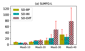
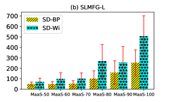
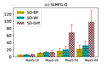
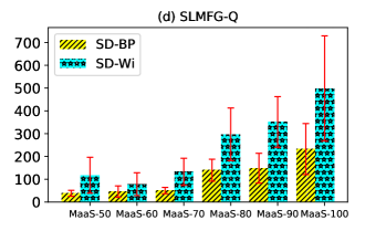
Figure 7: Average Runtime under different branching rules in $\bm{\mathsf{SD}}$-$\bm{\mathsf{B\&B}}$ algorithm for SLMFG-L and SLMFG-Q.

Observation 2

Compared with $\mathsf{Bard\&Moore}$ which exploits the explicit disjunctive structure of the complementarity conditions derived from a single violated complementarity condition, e.g., each of MPEC-L or MPEC-Q contains eight complementarity slackness conditions, the proposed SD-based B&B algorithms only branch once per follower problem, leading to a huge computational improvements, i.e., the runtime of $\mathsf{SD}$-$\mathsf{BP}$ is over 10 $\sim$ 100 times faster than that of $\mathsf{Bard\&Moore}$.

Observation 3

When the the scale of the instances is small, the CPU runtime of $\mathsf{SD}$-$\mathsf{Wi}$ is slightly smaller than its counterparts. when the scale of the instances is large, $\mathsf{SD}$-$\mathsf{BP}$ considerably outperforms the others for both SLMFGs.

Observation 4

Since LB is only updated if all follower problems are optimal. Hence, observe that even though in the quadratic case where SD-Q is a relaxation of SLMFG-Q using McCormick envelop, the value of leader’s objective value (LB) is same for four solution methods in each instance, confirming the effectiveness of proposed algorithm.

Observation 5

The profits of the MaaS regulator obtained in SLMFG with network effects (SLMFG-Q) is not greater than that in SLMFG without network effects (SLMFG-L). Moreover, these two formulations differ in the computational efforts required to solve the corresponding SLMFGs. Specifically, the average CPU runtime of SLMFG-Q is faster than that of SLMFG-L.

5.2 Sensitivity analysis

In this subsection, we conduct a sensitivity analysis on the parameters of the proposed SLMFG formulations. Algorithm $\mathsf{SD}$-$\mathsf{B\&B}$ with branching rule $\mathsf{SD}$-$\mathsf{BP}$ is used to solve all instances. We define the purchase-bidding price range ratio as the ratio of travelers’ maximum purchase-bidding price to the minimum purchase-bidding price $b_{max}/b_{min}$, and the sell-bidding price range ratio as the ratio of TSPs’ maximum sell-bidding price to the minimum sell-bidding price $\beta_{max}/\beta_{min}$. We conduct a sensitivity analysis on the bounds of the supply-demand gap, $[\underline{C},\bar{C}]$, where the upper bound $\bar{C}$ is the total capacity of mobility resources supplied by all TSPs and the lower bound $\underline{C}$ is the reserved capacity of MaaS regulator. We examine the behavior of the linear and quadratic cases, SLMFG-L and SLMFG-Q, for varying purchase-bid range ratio and sell-bid range ratio in Figure 8b and Figure 9b. We examine the behavior of the SLMFG-Q, for varying reserved capacity and total capacity in Figure 10b. We summarize the following insights which can be used as practical managerial guidelines:

Figure 8: Sensitivity analysis on purchase-bidding price range ratio $\bm{b_{max}/b_{min}}$

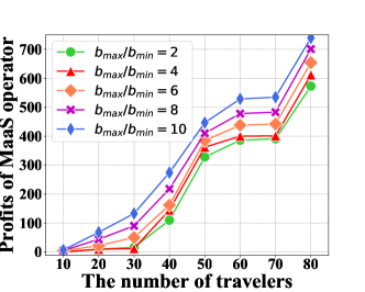
(a) SLMFG-L

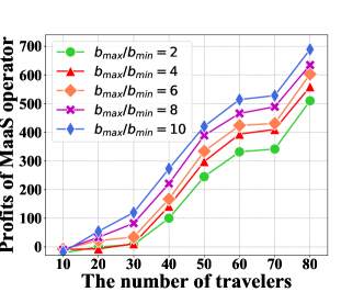
(b) SLMFG-Q

Figure 9: Sensitivity analysis on sell-bidding price range ratio $\bm{\beta_{max}/\beta_{min}}$

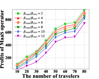
(a) SLMFG-L

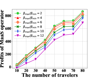
(b) SLMFG-Q

Figure 10: Sensitivity analysis on the lower and upper bound of $\Delta$ for SLMFG-Q.

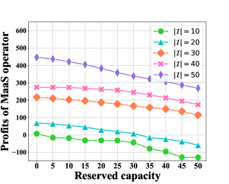
(a) Lower-bound of $\Delta$ ($\underline{C}$)

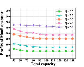
(b) Upper-bound of $\Delta$ ($\bar{C}$)

Observation 6

In SLMFG with/without network effects, an increase of the purchase-bidding price range ratio ($b_{\max}/b_{\min}$) leads to an increase in MaaS regulator’s profits for a fixed number of travelers, while an increase of the sell-bidding price range ratio ($\beta_{\max}/\beta_{\min}$) leads to a decrease in the MaaS regulator’s profits for a fixed number of TSPs. The profits of the MaaS regulator increase with the number of travelers (TSPs) under a fixed given purchase (sell)-bidding price range ratio.

Observation 7

In SLMFG with network effects, MaaS regulator’s profits will considerably decrease as $\underline{C}$ increases, and first slightly decrease and then keep unchanged as $\bar{C}$ increases. In SLMFG without network effects, the variation of $\underline{C}$ and $\bar{C}$ has no impacts on MaaS regulator’s profits.

6 Conclusion and remarks

In this study, we proposed a novel modeling and optimization framework for the regulation of two-sided MaaS markets. We cast this problem as a SLMFG where the leader is the MaaS regulator and two groups of followers are travelers and TSPs. We propose a NYOP-auction mechanism which allows travelers submit purchase-bids to fulfill their travel demand via MaaS platform and TSPs submit sell-bids to supply mobility resources for the MaaS platform simultaneously. We capture the network effects through the supply-demand in the two-sided MaaS markets, and consider SLMFG with and without network effects corresponding to MILBP and MIQBP problem, respectively. We provide constraint qualifications for MPEC reformulations of the both SLMFGs and prove the equivalence between the MPEC reformulations and their original problems, which lays a basis to develop solution algorithms based on the single-level reformulation of the SLMFGs. Further, we propose an exact solution method, SD-based B&B algorithm named $\mathsf{SD}$-$\mathsf{B\&B}$, which branches on accept/reject binary variables, and customize three rules to select branching variables. Our computational results show the performance of the proposed $\mathsf{SD}$-$\mathsf{B\&B}$ algorithms based on SD reformulation relative to a benchmark B&B algorithm based on MPEC reformulation and conclude that $\mathsf{SD}$-$\mathsf{BP}$ considerably outperforms the others for both SLMFGs, i.e., the computational speed of $\mathsf{SD}$-$\mathsf{BP}$ is over 10 $\sim$ 100 times faster than that of the benchmark when the scale of the instances is large. Our computational experiments uncover managerial insights into how the proposed SLMFGs behave in relation to the parameters, show that the MaaS regulator’s profits of the SLMFG with network effects are not greater than that of SLMFG without network effects, and indicate that both travelers’ travel costs and TSPs’ profits decrease with the increase of the supply-demand gap.

MaaS is a framework for delivering a portfolio of multi-modal mobility services that places user experience at the centre of the offer. Thus, instead of considering users’ mode choice across a set of travel modes, the proposed MaaS system unifies the mobility services provided by different travel modes as mobility resources and customize the optimal feasible MaaS bundles according to their WTP and experience-relevant requirements. Therefore, the NYOP-auction is perfectly adapted to the proposed user-centric MaaS framework. The results of this research provide managerial insights on how MaaS regulators make operational strategies (e.g., pricing and MaaS bundles) to attract price-sensitive travelers and TSPs with heterogeneous preference, WTP or WTS. Our findings also highlight how different stakeholders (MaaS regulator, travelers and TSPs) interact with each other to maximize their own benefits, notably the impact of cross-network effects on the profits of the MaaS regulator. This study suggests that MaaS platforms should consider cross network effects between travelers and TSPs to design their operational strategies.

This study can be extended in several research directions. The proposed SLMFG can be extended to multi-leader-follower problems to model the competition among different MaaS regulators. The proposed $\mathsf{SD}$-$\mathsf{B\&B}$ algorithm is applicable for any MIBLP/MIBQP with linear/quadratic follower problems. Future research is needed to explore stochastic formulations to capture the uncertainty in supply and demand, as well as the potential of time-varying pricing strategies.

Online Appendix for “Single-leader multi-follower games for the regulation of two-sided Mobility-as-a-Service markets”

7 Mathematical notations

Table 3: Parameters of the mathematical models

Parameters
$b_{i}$	Traveler $i$’s purchase-bidding price
$B_{i}$	Traveler $i$’s travel expenditure budget
$\bar{B}_{mn}$	TSP $mn$’s operating cost budget
$C_{mn}$	The capacity of the mobility resources provided by TSP $mn$
$\bar{C}$	Capacity of the mobility resources in the MaaS system provided by all TSPs, $C=\sum_{m\in\mathcal{M}}\sum_{n\in\mathcal{N}_{m}}C_{mn}$
$D_{i}$	Traveler $i$’s requested travel distance
$Q_{i}$	Traveler $i$’s requested quantity of mobility resources
$r_{i}$	Traveler $i$’s unit reserve price for mobility resources
${R}_{i}$	Traveler $i$’s maximum acceptable delay time during a mobility service (travel delay budget)
$T_{i}$	Traveler $i$’s requested total service time
$v_{m}$	Average commercial speed of travel mode $m$
$\alpha_{i}$	Traveler $i$’s unit waiting time cost
$\beta_{mn}$	TSP $mn$’s unit idle time cost
$\rho_{mn}$	TSP $mn$’s unit reserve price
$\Gamma_{i}$	Traveler $i$’s maximum acceptable inconvenience cost during a mobility service (inconvenience tolerance)
$\delta_{m}$	Inconvenience cost per unit of time for travel mode $m$
$\eta_{mn}$	TSP $mn$’s unit idle time cost
$\gamma_{mn}$	TSP $mn$’s unit operating cost
Decision variables
$p$	Real varible denoting the unit threshold price set for travelers using the MaaS platform
$q$	Real varible denoting the unit threshold price set for TSPs participating in the MaaS platform
$u_{i}$	Binary variable indicating whether Traveler $i$ is accepted to register MaaS platform or not
$w_{mn}$	Binary variable indicating whether the MaaS regulator offers TSP $mn$ to join the MaaS platform
$l_{i}^{m}$	Real variable denoting the service time of travel mode $m$ in the MaaS bundle allocated to Traveler $i$
$\Delta$	Real variable denoting supply-demand gap
$x_{i}$	Real varible representing the proportion mobility demand that $i$ chooses to use the MaaS platform
$y_{mn}$	Real variable representing the proportion of mobility resources to supply the MaaS platform
Sets
$\mathcal{I}$	Set of travelers, $\mathcal{I}=\left\{1,2,\cdots,i,\cdots,|\mathcal{I}|\right\}$
$\mathcal{M}$	Set of travel modes, $\mathcal{M}=\left\{1,2,\cdots,m,\cdots,|\mathcal{M}|\right\}$
$\mathcal{N}_{m}$	Set of TSPs of travel mode $m$, $\mathcal{N}_{m}=\left\{1,2,\cdots,n,\cdots,|\mathcal{N}_{m}|\right\},\forall m\in\mathcal{M}$

8 Equivalent formulations

8.1 Proof of Proposition 2

Proof 8.1

Proof: In SLMFG-L, since the objective function of travelers/TSPs has a separable structure and can be rewritten as:

$$G_{i}(x_{i},\Delta)=G_{i}^{1}(x_{i})+G_{i}^{2}(\Delta)\quad\mbox{ and }\quad H_{mn}(y_{mn},\Delta)=H_{mn}^{1}(y_{mn})+H_{mn}^{2}(\Delta),$$ (31)

where

$$G_{i}^{1}(x_{i})=b_{i}Q_{i}x_{i}+r_{i}Q_{i}(1-x_{i})-\frac{\alpha_{i}\zeta Q_{i}}{\bar{C}}x_{i},$$ (32a)

$$G_{i}^{2}(\Delta)=-\alpha_{i}\left(\frac{\zeta}{\bar{C}}\Delta+\vartheta\right),$$ (32b)

$$H_{mn}^{1}(y_{mn})=\left(\beta_{mn}-\rho_{mn}\right)C_{mn}y_{mn}+(\rho_{mn}-\gamma_{mn})C_{mn}(1-y_{mn})+\frac{\eta_{mn}\kappa C_{mn}}{\bar{C}}y_{mn},$$ (32c)

$$H_{mn}^{2}(\Delta)=-\eta_{mn}\left(\frac{\kappa}{\bar{C}}\Delta+\xi\right).$$ (32d)

As an immediate consequence, the solution set of the follower’s problem will not depend on the leader variable $\Delta$, we propose an equivalent formulation for SLMFG-L and state Proposition 1.

8.2 Proof of Proposition 3

Proof 8.2

Proof: For any feasible value of the leader’s variables $u_{i}$ and $w_{mn}$, the constraints set of the travelers and TSPs are nonempty, compact and their objective functions are continuous in their respective variables ($x_{i}$ and $y_{mn}$), therefore these follower problems admit at least a solution. Moreover, since the quadratic perceived waiting/idle functions ($\Psi_{i}^{q}(x_{i},\Delta)$ /($\Phi_{mn}^{q}(y_{mn},\Delta)$) are strictly convex, the objective functions of the travelers/TSPs are strictly convex/concave. Therefore, by classical uniqueness arguments, for any feasible value of the leader’s variables $u_{i}$ and $w_{mn}$, these follower problems admit a unique solution which can be denoted by $x_{i}(u_{i},\Delta)$ for Traveler $i$’s problem and by $y_{mn}(w_{mn},\Delta)$ for the TSP $mn$’s problem. Due to the uniqueness of the followers’ solutions, the optimistic approach used in Model 1 is no longer needed and SLMFG-Q is equivalent to SLMFG with network effects described in Proposition 3.3.

9 MPEC formulations

9.1 MPEC-L

$$0\leq(B_{i}-b_{i}Q_{i}x_{i})\perp\lambda_{1}^{i}\geq 0, \forall i\in\mathcal{I},$$ (KL.1)

$$0\leq\left(u_{i}-x_{i}\right)\perp\lambda_{2}^{i}\geq 0, \forall i\in\mathcal{I},$$ (KL.2)

$$0\leq x_{i}\perp\lambda_{3}^{i}\geq 0, \forall i\in\mathcal{I},$$ (KL.3)

$$0\leq\left[(b_{i}-r_{i})Q_{i}-\alpha_{i}\frac{\zeta}{\bar{C}}Q_{i}-\lambda_{1}^{i}b_{i}Q_{i}-\lambda_{2}^{i}+\lambda_{3}^{i}\right]\perp x_{i}\geq 0, \forall i\in\mathcal{I},$$ (KL.4)

where $\lambda_{1}^{i}$, $\lambda_{2}^{i}$ and $\lambda_{3}^{i}$ denote the Lagrangian multipliers associated with the constraints (T.2),(T.3) and (T.4), respectively. The operator ‘$a\perp b$’ denotes the complementarity condition $a\cdot b=0$.

The KKT conditions of TSP $mn$’s problem in SLMFG-Q are given in (KL.5)-(KL.8).

$$0\leq\left[\bar{B}_{mn}-C_{mn}\gamma_{mn}y_{mn}\right]\perp\mu_{1}^{mn}\geq 0, \forall m\in\mathcal{M},n\in\mathcal{N}_{m},$$ (KL.5)

$$0\leq(w_{mn}-y_{mn})\perp\mu_{2}^{mn}\geq 0, \forall m\in\mathcal{M},n\in\mathcal{N}_{m},$$ (KL.6)

$$0\leq y_{mn}\perp\mu_{3}^{mn}\geq 0, \forall m\in\mathcal{M},n\in\mathcal{N}_{m},$$ (KL.7)

$$0\leq\left[(\rho_{mn}-\beta_{mn})C_{mn}-\eta_{mn}\frac{\kappa}{\bar{C}}C_{mn}-\mu_{1}^{mn}C_{mn}\gamma_{mn}-\mu_{2}^{mn}+\mu_{3}^{mn}\right]$$

$$\perp y_{mn}\geq 0, \forall m\in\mathcal{M},n\in\mathcal{N}_{m},$$ (KL.8)

where $\mu_{1}^{mn}$, $\mu_{2}^{mn}$ and $\mu_{3}^{mn}$ denote the Lagrangian multipliers associated with constraint (P.2),(P.3) and (P.4), respectively.

9.2 MPEC-Q

The KKT conditions associated to Traveler $i$’s problem are given in (KQ.1)-(KQ.4):

$$0\leq(B_{i}-b_{i}Q_{i}x_{i})\perp\lambda_{1}^{i}\geq 0, \forall i\in\mathcal{I},$$ (KQ.1)

$$0\leq\left(u_{i}-x_{i}\right)\perp\lambda_{2}^{i}\geq 0, \forall i\in\mathcal{I},$$ (KQ.2)

$$0\leq x_{i}\perp\lambda_{3}^{i}\geq 0, \forall i\in\mathcal{I},$$ (KQ.3)

$$0\leq\left[\frac{2\zeta\alpha_{i}Q_{i}^{2}}{C^{2}}x_{i}-\left(\frac{2\zeta\alpha_{i}Q_{i}}{C}-\frac{2\zeta\alpha_{i}\Delta}{C^{2}}+r_{i}-b_{i}\right)Q_{i}-\lambda_{1}^{i}b_{i}Q_{i}-\lambda_{2}^{i}+\lambda_{3}^{i}\right]\perp x_{i}\geq 0, \forall i\in\mathcal{I},$$ (KQ.4)

where $\lambda_{1}^{i}$, $\lambda_{2}^{i}$ and $\lambda_{3}^{i}$ denotes the Lagrangian multipliers corresponding to the constraint (T.2),(T.3) and (T.4), respectively. On the other hand, $\forall m\in\mathcal{M},n\in\mathcal{N}_{m},$ the KKT conditions of the TSP $mn$’s follower- problem are given in (KQ.5)-(KQ.8).

$$0\leq\left[\bar{B}_{mn}-\beta_{mn}C_{mn}y_{mn}\right]\perp\mu_{1}^{mn}\geq 0, \forall m\in\mathcal{M},n\in\mathcal{N}_{m},$$ (KQ.5)

$$0\leq(w_{mn}-y_{mn})\perp\mu_{2}^{mn}\geq 0, \forall m\in\mathcal{M},n\in\mathcal{N}_{m},$$ (KQ.6)

$$0\leq y_{mn}\perp\mu_{3}^{mn}\geq 0, \forall m\in\mathcal{M},n\in\mathcal{N}_{m},$$ (KQ.7)

$$0\leq\Bigg{[}\frac{2\kappa\eta_{mn}C_{mn}^{2}}{C^{2}}y_{mn}-\left(\frac{2\kappa\eta_{mn}\Delta}{C^{2}}+\beta_{mn}-\rho_{mn}\right)C_{mn}$$

$$-\mu_{1}^{mn}\beta_{mn}C_{mn}-\mu_{2}^{mn}+\mu_{3}^{mn}\Bigg{]}\perp y_{mn}\geq 0, \forall m\in\mathcal{M},n\in\mathcal{N}_{m},$$ (KQ.8)

where $\mu_{1}^{mn}$, $\mu_{2}^{mn}$ and $\mu_{3}^{mn}$ denote the Lagrangian multipliers corresponding to the constraint (P.2),(P.3) and (P.4), respectively.

10 Proof of Theorem 1 (constraint qualifications)

The proof of Theorem 1 is based on Theorems 3.3.8 and 3.3.11 of Aussel and Svensson (2020). Let us first observe that SLMFG-L as described in Proposition 3.2 clearly satisfies the following basic properties:

• (Follower’s differentiability) $G_{i}(x_{i},\Delta)$ and $H_{mn}(y_{mn},\Delta)$ are differentiable;

• (Follower’s convexity) $G_{i}(x_{i},\Delta)$ and $H_{mn}(y_{mn},\Delta)$ are convex with respect to variables $x_{i}$ and $y_{mn}$ respectively.

Thus item $a)$ of Theorem 4.1 is a direct consequence of item i) of Aussel and Svensson (2020)[Theorem 3.3.8].

To prove item $b)$, let us now assume that for all traveler $i\in\mathcal{I}$, $b_{i}\geq p_{min}$ and for all TSP $n\in\mathcal{N}_{m},m\in\mathcal{M}$, $\beta_{mn}\leq q_{max}$. First the MILBP clearly satisfies the so-called Joint convexity assumption defined in Aussel and Svensson (2020) since all the constraint functions of the follower’s problem are linear.

Second, and in order to prove the Joint Slater’s qualification condition, let us first identify, in the forthcoming lemma, conditions under which a solution wherein all players of the market can participate.

Lemma 10.1

Let us assume that, for all Traveler $i\in\mathcal{I}$, $b_{i}\geq p_{min}$ and for all TSP $n\in\mathcal{N}_{m},m\in\mathcal{M}$, $\beta_{mn}\leq q_{max}$. Then there exists at least one feasible point of SLMFG-L such that $u_{i}=1$, for all Traveler $i\in\mathcal{I}$, and $w_{mn}=1$, for all TSP $n\in\mathcal{N}_{m},m\in\mathcal{M}$.

Proof 10.2

Proof: Observe that since $b_{i}\geq p_{min}$ for all Traveler $i\in\mathcal{I}$, if the leader chooses $p=p_{min}$, all travelers can participate, i.e. the couple $(p,u_{i})=(p_{min},1)$ satisfies Eqs. (M.6) and (M.7), for all $i\in\mathcal{I}$. Analogously, since $\beta_{mn}\leq q_{max}$ for all TSP $n\in\mathcal{N}_{m},m\in\mathcal{M}$, then if the leader chooses $q=q_{max}$, all TSPs can participate, i.e. the couple $(q,w_{mn})=(q_{max},1)$ satisfies Eqs. (M.8) and (M.9), for all $n\in\mathcal{N}_{m}$, $m\in\mathcal{M}$. Since variables $p$ and $q$ only appear in constraints (M.6)-(M.9), as well as in their bound constraints (M.13) and (M.14), respectively, the choice $p=p_{min}$ and $q=q_{max}$ is always feasible. In addition, let us recall that for any feasible value of the leader’s variables $u_{i}$, $w_{mn}$ and $\Delta$, the constraints set of the travelers and TSPs being nonempty compact and their objective function continuous in their respective variables ($x_{i}$ and $y_{mn}$), the followers’ problem admits at least a solution, respectively $\bar{\bm{x}}$ for travelers and $\bar{\bm{y}}$ for TSP. As a consequence the vector $(p_{min},q_{max},l,\bm{1},\bm{1},\Delta,\bar{\bm{x}},\bar{\bm{y}})$ is feasible for the SLMFG-L problem with $\bm{1}$ being vector $(1,\dots,1)$ and $(\bm{l},\Delta)$ satisfying Eqs. (M.2)-(M.5), (M.10), (M.15) and (M.16).

Now taking into account Lemma 10.1 and observing that, for any $i\in\mathcal{I}$, if $u_{i}=1$ then the constraint set of Traveler $i$’s problem is $[0,\min\{1,\frac{B_{i}}{b_{i}Q_{i}}\}]$ and for any $(m,n)\in\mathcal{M}\times\mathcal{N}$, if $w_{mn}=1$ then the constraint set of the TSP_mn’s problem is $[0,\min\{1,\frac{\bar{B}_{mn}}{C_{mn}\omega_{mn}}\}]$ one immediately deduces that the Joint Slater’s qualification condition needed in Aussel and Svensson (2020)[Theorem 3.3.11] is satisfied.

It remains to show that Guignard’s qualification conditions for boundary opponent strategies holds true. Let us precise that, according to Aussel and Svensson (2020)[Definition 3.3.10] and taking into account that the constraint set of the Traveler $i$ (respectively the TSP $mn$) only depends on $u_{i}$ (respectively $w_{mn}$), a boundary opponent strategy for traveler $i$ (respectively for TSP $mn$) is a point $(p,q,\bm{l},\bm{u},\bm{w},\Delta,\bm{x}_{-i},\bm{y})$ (respectively $(p,q,\bm{l},\bm{u},\bm{w},\Delta,\bm{x},\bm{y}_{-{mn}})$) such that $u_{i}=0$ or $u_{i}=1$ (respectively $w_{mn}=0$ or $w_{mn}=1$). Let us recall also that Guignard’s CQ is satisfied at $(p,q,\bm{l},\bm{u},\bm{w},\Delta,\bm{x},\bm{y})$ for follower $i$’s problem (respectively for follower $mn$’s problem) if

$$T^{o}(x_{i},(p,q,\bm{l},\bm{u},\bm{w},\Delta,\bm{x}_{-i},\bm{y}))=L^{o}(x_{i},(p,q,\bm{l},\bm{u},\bm{w},\Delta,\bm{x}_{-i},\bm{y}))$$

where $T^{o}(x_{i},(p,q,\bm{l},\bm{u},\bm{w},\Delta,\bm{x}_{-i},\bm{y}))$ stands for the Bouligand tangent cone at $x_{i}$ to the feasible set of traveler $i$’s problem parameterized by $(p,q,\bm{l},\bm{u},\bm{w},\Delta,\bm{x}_{-i},\bm{y})$ (actually parameterized by $u_{i}$) and $L^{o}(x_{i},(p,q,\bm{l},\bm{u},\bm{w},\Delta,\bm{x}_{-i},\bm{y}))$ denotes the polar to the linearized cone at $x_{i}$ of the feasible set of traveler $i$’s problem, which is defined by

$$\begin{array}[]{rcll}L(x_{i},(p,q,\bm{l},\bm{u},\bm{w},\Delta,\bm{x}_{-i},\bm{y}))&=&\left\{d\leavevmode\nobreak\ :\leavevmode\nobreak\ \right.&\langle\nabla g_{i}^{k}(x_{i},(p,q,\bm{l},\bm{u},\bm{w},\Delta,\bm{x}_{-i},\bm{y})),d\rangle\leq 0,\\[3.0pt] &&&\left.\forall\,k\mbox{ such that }g_{i}^{k}(x_{i},(p,q,\bm{l},\bm{u},\bm{w},\Delta,\bm{x}_{-i},\bm{y}))=0\right\}\end{array}$$

and the feasible set of Traveler i’s problem is defined as $\{x_{i}\leavevmode\nobreak\ :\leavevmode\nobreak\ g_{i}^{k}(x_{i},(p,q,\bm{l},\bm{u},\bm{w},\Delta,\bm{x}_{-i},\bm{y}))\leq 0,\leavevmode\nobreak\ k=1,\dots\}$. In our specific case the feasible set is defined by the following three linear functions $g_{i}^{1}(x_{i},u_{i})=b_{i}Q_{i}x_{i}-B_{i}$, $g_{i}^{2}(x_{i},u_{i})=-x_{i}$ and $g_{i}^{3}(x_{i},u_{i})=x_{i}-u_{i}$. Now if $u_{i}=0$ then the only feasible point of traveler $i$’s problem is $x_{i}=0$. In this case $\nabla g_{i}^{1}(0,0)=1$, $\nabla g_{i}^{2}(0,0)=-1$ and $\nabla g_{i}^{3}(0,0)=1$ therefore $L^{o}(x_{i},(p,q,\bm{l},(0,\bm{u}_{-i}),\bm{w},\Delta,\bm{x}_{-i},\bm{y}))=\mathbb{R}=T^{o}((x_{i},(p,q,\bm{l},(0,\bm{u}_{-i}),\bm{w},\Delta,\bm{x}_{-i},\bm{y}))$. Let us now consider the case $u_{i}=1$. In this case the feasible set of Traveler $i$’s problem is the interval $I=[0,\min\left\{1,\frac{B_{i}}{b_{i}Q_{i}}\right\}]$. For any $x\in]0,\min\left\{1,\frac{B_{i}}{b_{i}Q_{i}}\right\}[$, one clearly have that $g_{i}^{k}(x,(p,q,\bm{l},(0,\bm{u}_{-i}),\bm{w},\Delta,\bm{x}_{-i},\bm{y}))\neq 0$, for $k=1,2,3$ and thus $L((x_{i},(p,q,\bm{l},\bm{u},\bm{w},\Delta,\bm{x}_{-i},\bm{y}))=\mathbb{R}$. On the other hand $T^{o}(x_{i},(p,q,\bm{l},(0,\bm{u}_{-i}),\bm{w},\Delta,\bm{x}_{-i},\bm{y}))=\mathbb{R}$ and thus the desired equality holds true. Now if $x_{i}=0$ then only $g_{i}^{2}$ is null at $(0,1)$ and $\nabla g_{i}^{2}(0,1)=-1$ which implies that $L^{o}(0,(p,q,\bm{l},(1,\bm{u}_{-i}),\bm{w},\Delta,\bm{x}_{-i},\bm{y}))=\mathbb{R^{-}}=T^{o}(0,(p,q,\bm{l},(1,\bm{u}_{-i}),\bm{w},\Delta,\bm{x}_{-i},\bm{y}))$. Finally if $x_{i}=\min\left\{1,\frac{B_{i}}{b_{i}Q_{i}}\right\}$ then one (and only one) of the functions $g_{i}^{1}$ or $g_{i}^{3}$ is null at $(x_{i},1)$. Since $\nabla g_{i}^{1}(x_{i},1)=1=\nabla g_{i}^{3}(x_{i},1)=1$, then one has again $L^{o}(x_{i},(p,q,\bm{l},(1,\bm{u}_{-i}),\bm{w},\Delta,\bm{x}_{-i},\bm{y}))=\mathbb{R^{-}}=T^{o}(x_{i},(p,q,\bm{l},(1,\bm{u}_{-i}),\bm{w},\Delta,\bm{x}_{-i},\bm{y}))$. The same reasoning will work for the TSP $mn$’s problem. We can thus conclude that Guignard’s CQ is satisfied at any boundary opponent strategy. All assumptions of Aussel and Svensson (2020)[Theorem 3.3.11] are fulfilled and thus item $b)$ of Theorem 4.1 is proved.

11 SD reformulation

11.1 Proof of Corollary 1

Corollary 11.1

Assume that the perceived waiting/idle time functions of followers are linear.

• If $(p,q,\bm{l},\bm{u},\bm{w},\Delta,\bm{x},\bm{y})$ is a global solution of SLMFG-L, then $\forall(\bm{\bar{\lambda}},\bm{\bar{\mu}})\in\bar{\Lambda}(p,q,\bm{l},\bm{u},\bm{w},\Delta,\bm{x},\bm{y})$, $(p,q,\bm{l},\bm{u},\bm{w},\Delta,\bm{x},\bm{y},\bm{\bar{\lambda}},\bm{\bar{\mu}})$ is a global solution of the associated SD-based reformulation SD-L.

• Assume additionally that

  • for all Traveler $i\in\mathcal{I}$, $b_{i}\geq p_{min}$;

  • for all TSP $n\in\mathcal{N}_{m},m\in\mathcal{M}$, $\beta_{mn}\leq q_{max}$.

  If $(p,q,\bm{l},\bm{u},\bm{w},\Delta,\bm{x},\bm{y},\bm{\bar{\lambda}},\bm{\bar{\mu}})$ is a global solution of SD-L, then $(p,q,\bm{l},\bm{u},\bm{w},\Delta,\bm{x},\bm{y})$ is a global solution of SLMFG-L.

11.2 primal-dual formulations of SLMFG-Q

To simplify the derivation, we convert each TSP’s maximization problem into a minimization problem and give primal-dual formulations of SLMFG-Q as follows.

Lemma 11.2

The dual problem of $G_{i}$ can be written as:

$$\quad\max_{\bm{\lambda}}\quad\ -\frac{1}{2P_{i}}\left[(A_{i}\bar{\lambda}_{1}^{i})^{2}+(\bar{\lambda}_{2}^{i})^{2}\right]-\frac{U_{i}}{P_{i}}\left(A_{i}\bar{\lambda}_{1}^{i}+\bar{\lambda}_{2}^{i}\right)-\frac{1}{P_{i}}\left(A_{i}\bar{\lambda}_{1}^{i}\bar{\lambda}_{2}^{i}\right)-\frac{U_{i}^{2}}{2P_{i}}-B_{i}\bar{\lambda}_{1}^{i}-\bar{\lambda}_{2}^{i}u_{i}$$ (37a)

subject to

$$\bar{\lambda}_{1}^{i},\bar{\lambda}_{2}^{i}\geq 0,$$ (37b)

where $A_{i}=b_{i}Q_{i}$, $U_{i}=-\left(\frac{2\zeta\alpha_{i}Q_{i}}{\bar{C}}-\frac{2\zeta\alpha_{i}\Delta}{C^{2}}+r_{i}-b_{i}\right)Q_{i}$, $1/P_{i}=\frac{C^{2}}{2\zeta\alpha_{i}Q_{i}^{2}}$, and $\bar{\lambda}_{1}^{i}$ and $\bar{\lambda}_{2}^{i}$ are the dual variables corresponding to constraints (T.2) and (T.3), respectively.

The dual problem of $H_{mn}$ can be written as:

$$\max_{\bm{\mu}}\quad-\frac{1}{2P_{mn}}\left[(A_{mn}\bar{\mu}_{1}^{mn})^{2}+(\bar{\mu}_{2}^{mn})^{2}\right]-\frac{U_{mn}}{P_{mn}}\left(A_{mn}\bar{\mu}_{1}^{mn}+\bar{\mu}_{2}^{mn}\right)-\frac{1}{P_{mn}}(A_{mn}\bar{\mu}_{1}^{mn}\bar{\mu}_{2}^{mn})$$

$$-\frac{U_{mn}^{2}}{2P_{mn}}-\bar{B}_{mn}\bar{\mu}_{1}^{mn}-w_{mn}\bar{\mu}_{2}^{mn}$$ (38a)

subject to

$$\bar{\mu}_{1}^{mn},\bar{\mu}_{2}^{mn}\geq 0,$$ (38b)

where $A_{mn}=C_{mn}\gamma_{mn}$, $U_{mn}=-\left(\frac{2\kappa\eta_{mn}\Delta}{C^{2}}+\beta_{mn}-\rho_{mn}\right)C_{mn}$, and $1/P_{mn}=\frac{C^{2}}{2\kappa\eta_{mn}C_{mn}^{2}}$, and $\bar{\mu}_{1}^{mn}$ and $\bar{\mu}_{2}^{mn}$ are the dual variables corresponding to constraints (P.2) and (P.3), respectively.

Proof 11.3

Proof: Followers’ primal problem are summarized in Eqs. (39a)-(39d):

$$(\text{Primal problem}):\quad\min_{\bm{x}}\quad\frac{1}{2}\bm{x}^{T}\mathbf{P}\bm{x}+\mathbf{U}^{T}\bm{x},$$ (39a)

subject to:

$$\quad\quad\hskip 76.82234pt\mathbf{A}\bm{x}\leq\mathbf{b},$$ (39b)

$$\quad\quad\hskip 76.82234pt\bm{x}\leq\bm{u},$$ (39c)

$$\quad\quad\hskip 76.82234pt\bm{x}\geq\mathbf{0}.$$ (39d)

The Lagrangian function is given in Eq.(40):

$$\mathcal{L}_{1}(\bm{x},\bm{\lambda_{1}},\bm{\lambda_{2}},\bm{\lambda_{3}})=\inf_{\bm{x}}\left\{\frac{1}{2}\bm{x}^{T}\bm{P}\bm{x}+\bm{U}^{T}\bm{x}+\bm{\lambda_{1}}^{T}(\bm{A}\bm{x}-\bm{b})+\bm{\lambda_{2}}^{T}(\bm{x}-\bm{\mu})-\bm{\lambda_{3}}^{T}\bm{x}\right\},$$ (40)

where $\bm{\lambda_{1}}$, $\bm{\lambda_{2}}$ and $\bm{\lambda_{3}}$ denotes the Lagrangian multipliers corresponding to constraint (39b)-(39d), respectively.

The dual problem is then given in Eqs. (41a)-(41c):

$$\max_{\bm{\lambda_{1}},\bm{\lambda_{2}},\bm{\lambda_{3}}}\quad\left\{\min_{\bm{x}}\mathcal{L}_{1}(\bm{x},\bm{\lambda_{1}},\bm{\lambda_{2}},\bm{\lambda_{3}})\right\},$$ (41a)

subject to:

$$\frac{\partial\mathcal{L}_{1}(\bm{x},\bm{\lambda_{1}},\bm{\lambda_{2}},\bm{\lambda_{3}})}{\partial\bm{x}}=\mathbf{P}\bm{x}+\mathbf{U}+\mathbf{A}^{T}\bm{\lambda_{1}}+\bm{\lambda_{2}}-\bm{\lambda_{3}}=\mathbf{0},$$ (41b)

$$\bm{\lambda_{1}},\bm{\lambda_{2}},\bm{\lambda_{3}}\geq 0.$$ (41c)

The dual constraint (41b) implies that $\bm{x}^{T}[\mathbf{P}\bm{x}+\mathbf{U}+\mathbf{A}^{T}\bm{\lambda_{1}}+\bm{\lambda_{2}}-\bm{\lambda_{3}}]=\bm{x}^{T}\mathbf{0}$, namely,

$$\bm{x}^{T}\mathbf{P}\bm{x}+\bm{x}^{T}\mathbf{U}+\bm{\lambda_{1}}^{T}\mathbf{A}\bm{x}+\bm{\lambda_{2}}^{T}\bm{x}-\bm{\lambda_{3}}^{T}\bm{x}=\mathbf{0}.$$ (42)

Thus the dual objective (41a) can be written as:

$$-\frac{1}{2}\bm{x}^{T}\mathbf{P}\bm{x}-\bm{\lambda_{1}}^{T}\mathbf{b}-\bm{\lambda_{2}}^{T}\bm{u}+(\bm{x}^{T}\mathbf{P}\bm{x}+\bm{x}^{T}\mathbf{U}+\bm{\lambda_{1}}^{T}\mathbf{A}\bm{x}+\bm{\lambda_{2}}^{T}\bm{x}-\bm{\lambda_{3}}^{T}\bm{x}).$$ (43)

Then the dual problem of Eqs.(39a)-(39d) is given in Eqs. (44a)-(44c):

$$(\text{Dual problem}):\quad\max_{\bm{\lambda_{1},\bm{\lambda_{2}}}}\quad-\frac{1}{2}\bm{x}^{T}\mathbf{P}\bm{x}-\bm{\lambda_{1}}^{T}\mathbf{b}-\bm{\lambda_{2}}^{T}\bm{u},$$ (44a)

subject to:

$$\quad\quad\hskip 68.28644pt\mathbf{P}\bm{x}+\mathbf{U}+\mathbf{A}^{T}\bm{\lambda_{1}}+\bm{\lambda_{2}}=\mathbf{0},$$ (44b)

$$\quad\quad\hskip 68.28644pt\bm{\lambda_{1}},\bm{\lambda_{2}}\geq\mathbf{0}.$$ (44c)

Since $\mathbf{P}^{-1}$ exists, from the dual constraints we have:

$$\mathbf{P}\bm{x}+\mathbf{U}+\mathbf{A}^{T}\bm{\lambda_{1}}+\bm{\lambda_{2}}=\mathbf{0}\Longrightarrow\bm{x}+\mathbf{P}^{-1}\mathbf{U}+\mathbf{P}^{-1}\mathbf{A}^{T}\bm{\lambda_{1}}+\mathbf{P}^{-1}\bm{\lambda_{2}}=\mathbf{0},$$ (45)

i.e.,

$$\bm{x}=-\mathbf{P}^{-1}\left(\bm{\mathbf{U}}+\mathbf{A}^{T}\bm{\lambda_{1}}+\bm{\lambda_{2}}\right).$$ (46)

Then, substituting Eq.(46) into the dual objective function (44a) and rearranging, we obtain:

$$-\frac{1}{2}\bm{x}^{T}\mathbf{P}\bm{x}-\bm{\lambda_{1}}^{T}\mathbf{b}-\bm{\lambda_{2}}^{T}\bm{u}$$ (47a)

$$=-\frac{1}{2}[\mathbf{P}^{-1}\left(\bm{\mathbf{U}}+\mathbf{A}^{T}\bm{\lambda_{1}}+\bm{\lambda_{2}}\right)^{T}]\cdot\mathbf{P}\cdot[\mathbf{P}^{-1}\left(\bm{\mathbf{U}}+\mathbf{A}^{T}\bm{\lambda_{1}}+\bm{\lambda_{2}}\right)]-\mathbf{b}^{T}\bm{\lambda_{1}}-\mathbf{u}^{T}\bm{\lambda_{2}}$$ (47b)

$$=-\frac{1}{2}\left(\bm{\mathbf{U}}^{T}+\bm{\lambda_{1}}^{T}\mathbf{A}+\bm{\lambda_{2}}^{T}\right)\cdot\mathbf{P}^{-1}\cdot\left(\bm{\mathbf{U}}+\mathbf{A}^{T}\bm{\lambda_{1}}+\bm{\lambda_{2}}\right)-\mathbf{b}^{T}\bm{\lambda_{1}}-\mathbf{u}^{T}\bm{\lambda_{2}}$$ (47c)

$$=-\frac{1}{2}\left(\bm{\mathbf{U}}^{T}\mathbf{P}^{-1}+\bm{\lambda_{1}}^{T}\mathbf{A}\mathbf{P}^{-1}+\bm{\lambda_{2}}^{T}\mathbf{P}^{-1}\right)\cdot\left(\bm{\mathbf{U}}+\mathbf{A}^{T}\bm{\lambda_{1}}+\bm{\lambda_{2}}\right)-\mathbf{b}^{T}\bm{\lambda_{1}}-\mathbf{u}^{T}\bm{\lambda_{2}}$$ (47d)

$$=-\frac{1}{2}(\bm{\lambda_{1}}^{T}\mathbf{A}\mathbf{P}^{-1}\mathbf{A}^{T}\bm{\lambda_{1}}+\bm{\lambda_{2}}^{T}\mathbf{P}^{-1}\bm{\lambda_{2}})-\frac{1}{2}(2\bm{\mathbf{U}}^{T}\mathbf{P}^{-1}\mathbf{A}^{T}\bm{\lambda_{1}}+2\bm{\mathbf{U}}^{T}\mathbf{P}^{-1}\bm{\lambda_{2}}+2\bm{\lambda_{1}}^{T}\mathbf{A}\mathbf{P}^{-1}{\bm{\lambda_{2}}})$$

$$-\frac{1}{2}\bm{\mathbf{U}}^{T}\mathbf{P}^{-1}\bm{\mathbf{U}}-\mathbf{b}^{T}\bm{\lambda_{1}}-\mathbf{u}^{T}\bm{\lambda_{2}}$$ (47e)

$$=-\frac{1}{2}(\bm{\lambda_{1}}^{T}\mathbf{A}\mathbf{P}^{-1}\mathbf{A}^{T}\bm{\lambda_{1}}+\bm{\lambda_{2}}^{T}\mathbf{P}^{-1}\bm{\lambda_{2}})-(\bm{\mathbf{U}}^{T}\mathbf{P}^{-1}\mathbf{A}^{T}\bm{\lambda_{1}}+\bm{\mathbf{U}}^{T}\mathbf{P}^{-1}\bm{\lambda_{2}}+\bm{\lambda_{1}}^{T}\mathbf{A}\mathbf{P}^{-1}{\bm{\lambda_{2}}})$$

$$-\frac{1}{2}\bm{\mathbf{U}}^{T}\mathbf{P}^{-1}\bm{\mathbf{U}}-\mathbf{b}^{T}\bm{\lambda_{1}}-\mathbf{u}^{T}\bm{\lambda_{2}}.$$ (47f)

The dual problem can be written as:

$$\min_{\bm{\lambda_{1}},\bm{\lambda_{2}}}\quad-\frac{1}{2}\mathbf{P}^{-1}(\bm{\lambda_{1}}^{T}\mathbf{A}\mathbf{A}^{T}\bm{\lambda_{1}}+\bm{\lambda_{2}}^{T}\bm{\lambda_{2}})-\mathbf{U}^{T}\mathbf{P}^{-1}(\mathbf{A}^{T}\bm{\lambda_{1}}+\bm{\lambda_{2}})-\bm{\lambda_{1}}^{T}\mathbf{A}\mathbf{P}^{-1}{\bm{\lambda_{2}}}-\frac{1}{2}\bm{\mathbf{U}}^{T}\mathbf{P}^{-1}\bm{\mathbf{U}}-\mathbf{b}^{T}\bm{\lambda_{1}}-\mathbf{u}^{T}\bm{\lambda_{2}},$$ (48a)

subject to:

$$\bm{\lambda_{1}},\bm{\lambda_{2}}\geq\mathbf{0}.$$ (48b)

Thus concluding the proof.

11.3 Proof of Corollary 2

In Corollary 11.1, the set $\bar{\Lambda}(\cdot)$ stands for the set of dual variables associated to the SD conditions of the followers (travelers and TSPs).

Corollary 11.4

Assume that the perceived waiting/idle time functions of followers are quadratic.

• If $(p,q,\bm{l},\bm{u},\bm{w},\Delta,\bm{x},\bm{y})$ is a global solution of SLMFG-Q, then $\forall(\bm{\bar{\lambda}},\bm{\bar{\mu}})\in\bar{\Lambda}(p,q,\bm{l},\bm{u},\bm{w},\Delta,\bm{x},\bm{y})$, $(p,q,\bm{l},\bm{u},\bm{w},\Delta,\bm{x},\bm{y},\bm{\bar{\lambda}},\bm{\bar{\mu}})$ is a global solution of the associated SD-based reformulation SD-Q.

• Assume additionally that

  • for all Traveler $i\in\mathcal{I}$, $b_{i}\geq p_{min}$;

  • for all TSP $n\in\mathcal{N}_{m},m\in\mathcal{M}$, $\beta_{mn}\leq q_{max}$.

  If $(p,q,\bm{l},\bm{u},\bm{w},\Delta,\bm{x},\bm{y},\bm{\bar{\lambda}},\bm{\bar{\mu}})$ is a global solution of SD-Q, then $(p,q,\bm{l},\bm{u},\bm{w},\Delta,\bm{x},\bm{y})$ is a global solution of SLMFG-Q.

11.4 McCormick envelope relaxation

We relax these bilinear terms by introducing auxiliary variables $W_{i}\triangleq\Delta\cdot x_{i}$ and $W_{mn}\triangleq\Delta\cdot y_{mn}$ using their McCormick envelopes (McCormick 1976). Accordingly, constraints (MK.1)-(MK.8) are added to the SD reformulation of SLMFG-Q.

$$0\leq W_{i}\leq C, \forall i\in\mathcal{I},$$ (MK.1)

$$W_{i}\geq\Delta+Cx_{i}-C, \forall i\in\mathcal{I},$$ (MK.2)

$$W_{i}\leq\Delta+\underline{C}x_{i}-\underline{C}, \forall i\in\mathcal{I},$$ (MK.3)

$$W_{i}\leq Cx_{i}, \forall i\in\mathcal{I},$$ (MK.4)

$$0\leq W_{mn}\leq C, m\in\mathcal{M},n\in\mathcal{N}_{m},$$ (MK.5)

$$W_{mn}\geq\Delta+Cy_{mn}-C, m\in\mathcal{M},n\in\mathcal{N}_{m},$$ (MK.6)

$$W_{mn}\leq\Delta+\underline{C}y_{mn}-\underline{C}, m\in\mathcal{M},n\in\mathcal{N}_{m},$$ (MK.7)

$$W_{mn}\leq Cy_{mn}, m\in\mathcal{M},n\in\mathcal{N}_{m},$$ (MK.8)

12 Formulations of the sub-problems

(The $\bm{kth}$ sub-problem $\textit{SP}^{k}$ of SLMFG-L)

$$\max_{p,q,\bm{l},\bm{u},\bm{\tau},\Delta,\bm{x},\bm{y}}F=\sum_{i\in\mathcal{I}}b_{i}Q_{i}x_{i}-\sum_{m\in\mathcal{M}}\sum_{n\in\mathcal{N}_{m}}\beta_{mn}c_{mn}y_{mn},$$ (M.1)

subject to:

MaaS regulator’s constraints:

$$\sum_{m\in\mathcal{M}}v_{m}l_{i}^{m}=D_{i}x_{i}, \forall i\in\mathcal{I},$$ (M.2)

$$0\leq\sum_{m\in\mathcal{M}}l_{i}^{m}-T_{i}x_{i}\leq{R}_{i}, \forall i\in\mathcal{I},$$ (M.3)

$$\sum_{m\in\mathcal{M}}\sigma_{m}l_{i}^{m}\leq\Gamma_{i}, \forall i\in\mathcal{I},$$ (M.4)

$$\sum_{i\in\mathcal{I}}v_{m}^{2}l_{i}^{m}\leq\sum_{n\in\mathcal{N}_{m}}C_{mn}y_{mn}, \forall m\in\mathcal{M},$$ (M.5)

$$b_{i}-p\geq(1-u_{i})(b_{i}-p_{max}), \forall i\in\mathcal{I},$$ (M.6)

$$b_{i}-p\leq u_{i}(b_{i}-p_{min}), \forall i\in\mathcal{I},$$ (M.7)

$$q-\beta_{mn}\geq(1-w_{mn})(q_{min}-\beta_{mn}), \forall m\in\mathcal{M},n\in\mathcal{N}_{m},$$ (M.8)

$$q-\beta_{mn}\leq w_{mn}(q_{max}-\beta_{mn}), \forall m\in\mathcal{M},n\in\mathcal{N}_{m},$$ (M.9)

$$\Delta=\sum_{m\in\mathcal{M}}\sum_{n\in\mathcal{N}_{m}}C_{mn}y_{mn}-\sum_{i\in\mathcal{I}}Q_{i}x_{i},$$ (M.10)

$$u_{i}\in\left\{0,1\right\}, \forall i\in\mathcal{I},$$ (M.11)

$$w_{mn}\in\left\{0,1\right\}, \forall m\in\mathcal{M},n\in\mathcal{N}_{m},$$ (M.12)

$$l_{i}^{m}\geq 0, \forall i\in\mathcal{I},m\in\mathcal{M},$$ (M.13)

$$p_{min}\leq p\leq p_{max},$$ (M.14)

$$q_{min}\leq q\leq q_{max},$$ (M.15)

$$\underline{C}\leq\Delta\leq\overline{C},$$ (M.16)

SD conditions of travelers:

$$b_{i}Q_{i}x_{i}\leq B_{i}, \forall i\in\mathcal{I},$$ (T.2)

$$x_{i}\leq u_{i}, \forall i\in\mathcal{I},$$ (T.3)

$$x_{i}\geq 0, \forall i\in\mathcal{I},$$ (T.4)

$$u_{i}=0, \forall i\in\overline{\mathcal{I}}_{0}^{k},$$ (50a)

$$u_{i}=1, \forall i\in\overline{\mathcal{I}}_{1}^{k},$$ (50b)

$$(r_{i}-b_{i})Q_{i}x_{i}\geq B_{i}\bar{\lambda}_{1}^{i}+u_{i}\bar{\lambda}_{2}^{i}, \forall i\in\overline{\mathcal{I}}_{1}^{k},$$ (50c)

$$b_{i}Q_{i}\bar{\lambda}_{1}^{i}+\bar{\lambda}_{2}^{i}\geq(r_{i}-b_{i})Q_{i}, \forall i\in\overline{\mathcal{I}}_{1}^{k},$$ (50d)

$$\bar{\lambda}_{1}^{i},\bar{\lambda}_{2}^{i}\geq 0, \forall i\in\overline{\mathcal{I}}_{1}^{k},$$ (50e)

SD conditions of TSPs:

$$C_{mn}\gamma_{mn}y_{mn}\leq\bar{B}_{mn}, \forall(m,n)\in\mathcal{MN},$$ (P.2)

$$y_{mn}\leq w_{mn}, \forall(m,n)\in\mathcal{MN},$$ (P.3)

$$y_{mn}\geq 0, \forall(m,n)\in\mathcal{MN},$$ (P.4)

$$\tau_{mn}=0, \forall(m,n)\in\overline{\mathcal{MN}}_{0}^{k},$$ (50f)

$$\tau_{mn}=1, \forall(m,n)\in\overline{\mathcal{MN}}_{1}^{k},$$ (50g)

$$(\beta_{mn}-\rho_{mn})c_{mn}y_{mn}\geq\bar{B}_{mn}\bar{\mu}_{1}^{mn}+\tau_{mn}\bar{\mu}_{2}^{mn}, \forall(m,n)\in\overline{\mathcal{MN}}_{1}^{k},$$ (50h)

$$c_{mn}\gamma_{mn}\bar{\mu}_{1}^{mn}+\bar{\mu}_{2}^{mn}\geq(\beta_{mn}-\rho_{mn})c_{mn}, \forall(m,n)\in\overline{\mathcal{MN}}_{1}^{k},$$ (50i)

$$\bar{\mu}_{1}^{mn},\bar{\mu}_{2}^{mn}\geq 0, \forall(m,n)\in\overline{\mathcal{MN}}_{1}^{k},$$ (50j)

(The $\bm{kth}$ sub-problem $\textit{SP}^{k}$ of SLMFG-Q)

$$\max_{p,q,\bm{l},\bm{u},\bm{\tau},\Delta,\bm{x},\bm{y}}F=\sum_{i\in\mathcal{I}}b_{i}Q_{i}x_{i}-\sum_{m\in\mathcal{M}}\sum_{n\in\mathcal{N}_{m}}\beta_{mn}c_{mn}y_{mn},$$ (51a)

subject to:

MaaS regulator’s constraints:

$$\sum_{m\in\mathcal{M}}v_{m}l_{i}^{m}=D_{i}x_{i}, \forall i\in\mathcal{I},$$ (M.2)

$$0\leq\sum_{m\in\mathcal{M}}l_{i}^{m}-T_{i}x_{i}\leq{R}_{i}, \forall i\in\mathcal{I},$$ (M.3)

$$\sum_{m\in\mathcal{M}}\sigma_{m}l_{i}^{m}\leq\Gamma_{i}, \forall i\in\mathcal{I},$$ (M.4)

$$\sum_{i\in\mathcal{I}}v_{m}^{2}l_{i}^{m}\leq\sum_{n\in\mathcal{N}_{m}}C_{mn}y_{mn}, \forall m\in\mathcal{M},$$ (M.5)

$$b_{i}-p\geq(1-u_{i})(b_{i}-p_{max}), \forall i\in\mathcal{I},$$ (M.6)

$$b_{i}-p\leq u_{i}(b_{i}-p_{min}), \forall i\in\mathcal{I},$$ (M.7)

$$q-\beta_{mn}\geq(1-w_{mn})(q_{min}-\beta_{mn}), \forall m\in\mathcal{M},n\in\mathcal{N}_{m},$$ (M.8)

$$q-\beta_{mn}\leq w_{mn}(q_{max}-\beta_{mn}), \forall m\in\mathcal{M},n\in\mathcal{N}_{m},$$ (M.9)

$$\Delta=\sum_{m\in\mathcal{M}}\sum_{n\in\mathcal{N}_{m}}C_{mn}y_{mn}-\sum_{i\in\mathcal{I}}Q_{i}x_{i},$$ (M.10)

$$u_{i}\in\left\{0,1\right\}, \forall i\in\mathcal{I},$$ (M.11)

$$w_{mn}\in\left\{0,1\right\}, \forall m\in\mathcal{M},n\in\mathcal{N}_{m},$$ (M.12)

$$l_{i}^{m}\geq 0, \forall i\in\mathcal{I},m\in\mathcal{M},$$ (M.13)

$$p_{min}\leq p\leq p_{max},$$ (M.14)

$$q_{min}\leq q\leq q_{max},$$ (M.15)

$$\underline{C}\leq\Delta\leq\overline{C},$$ (M.16)

SD conditions of travelers:

$$b_{i}Q_{i}x_{i}\leq B_{i}, \forall i\in\mathcal{I},$$ (T.2)

$$x_{i}\leq u_{i}, \forall i\in\mathcal{I},$$ (T.3)

$$x_{i}\geq 0, \forall i\in\mathcal{I},$$ (T.4)

$$u_{i}=0, \forall i\in\overline{\mathcal{I}}_{0}^{k},$$ (51b)

$$u_{i}=1, \forall i\in\overline{\mathcal{I}}_{1}^{k},$$ (51c)

$$\frac{\zeta\alpha_{i}Q_{i}^{2}}{C^{2}}x_{i}^{2}-\left(\frac{2\zeta\alpha_{i}Q_{i}}{\bar{C}}-\frac{2\zeta\alpha_{i}\Delta}{C^{2}}+r_{i}-b_{i}\right)Q_{i}x_{i}\leq-\frac{(A_{i}\bar{\lambda}_{1}^{i})^{2}+(\bar{\lambda}_{2}^{i})^{2}}{2P_{i}}$$

$$-\frac{U_{i}}{P_{i}}\left(b_{i}Q_{i}\bar{\lambda}_{1}^{i}+\bar{\lambda}_{2}^{i}\right)-\frac{b_{i}Q_{i}\bar{\lambda}_{1}^{i}\bar{\lambda}_{2}^{i}}{P_{i}}-\frac{U_{i}^{2}}{2P_{i}}-B_{i}\bar{\lambda}_{1}^{i}-\bar{\lambda}_{2}^{i}u_{i}, \forall i\in\overline{\mathcal{I}}_{1}^{k},$$ (51d)

$$\bar{\lambda}_{1}^{i},\bar{\lambda}_{2}^{i}\geq 0, \forall i\in\overline{\mathcal{I}}_{1}^{k},$$ (51e)

McCormick envelopes Relaxation:

$$0\leq W_{i}\leq C, \forall i\in\mathcal{I},$$ (MK.1)

$$W_{i}\geq\Delta+Cx_{i}-C, \forall i\in\overline{\mathcal{I}}_{1}^{k},$$ (MK.2)

$$W_{i}\leq\Delta+\underline{C}x_{i}-\underline{C}, \forall i\in\overline{\mathcal{I}}_{1}^{k},$$ (MK.3)

$$W_{i}\leq Cx_{i}, \forall i\in\overline{\mathcal{I}}_{1}^{k},$$ (MK.4)

SD conditions of TSPs:

$$C_{mn}\gamma_{mn}y_{mn}\leq\bar{B}_{mn}, \forall(m,n)\in\mathcal{MN},$$ (P.2)

$$y_{mn}\leq w_{mn}, \forall(m,n)\in\mathcal{MN},$$ (P.3)

$$y_{mn}\geq 0, \forall(m,n)\in\mathcal{MN},$$ (P.4)

$$\tau_{mn}=0, \forall(m,n)\in\overline{\mathcal{MN}}_{0}^{k},$$ (51f)

$$\tau_{mn}=1, \forall(m,n)\in\overline{\mathcal{MN}}_{1}^{k},$$ (51g)

$$\frac{\kappa\eta_{mn}C_{mn}^{2}}{C^{2}}y_{mn}^{2}-\left(\frac{2\kappa\eta_{mn}\Delta}{C^{2}}+\beta_{mn}-\rho_{mn}\right)C_{mn}y_{mn}\leq$$

$$-\frac{(A_{mn}\bar{\mu}_{1}^{mn})^{2}+(\bar{\mu}_{2}^{mn})^{2}}{2P_{mn}}-\frac{U_{mn}}{P_{mn}}\left(A_{mn}\bar{\mu}_{1}^{mn}+\bar{\mu}_{2}^{mn}\right)-\frac{A_{mn}\bar{\mu}_{1}^{mn}\bar{\mu}_{2}^{mn}}{P_{mn}}$$

$$-\frac{U_{mn}^{2}}{2P_{mn}}-\bar{B}_{mn}\bar{\mu}_{1}^{mn}-w_{mn}\bar{\mu}_{2}^{mn}, \forall(m,n)\in\overline{\mathcal{MN}}_{1}^{k},$$ (51h)

$$\bar{\mu}_{1}^{mn},\bar{\mu}_{2}^{mn}\geq 0, \forall(m,n)\in\overline{\mathcal{MN}}_{1}^{k},$$ (51i)

McCormick envelopes Relaxation:

$$0\leq W_{mn}\leq C, \forall(m,n)\in\overline{\mathcal{MN}}_{1}^{k},$$ (MK.5)

$$W_{mn}\geq\Delta+Cy_{mn}-C, \forall(m,n)\in\overline{\mathcal{MN}}_{1}^{k},$$ (MK.6)

$$W_{mn}\leq\Delta+\underline{C}y_{mn}-\underline{C}, \forall(m,n)\in\overline{\mathcal{MN}}_{1}^{k},$$ (MK.7)

$$W_{mn}\leq Cy_{mn}, \forall(m,n)\in\overline{\mathcal{MN}}_{1}^{k},$$ (MK.8)

13 Computation study

13.1 Input data

MaaS requests of both travelers and TSPs are input information to the proposed two-sided MaaS market. To obtain travelers’ and TSPs’ request data, we conduct stochastic simulations on travelers and TSPs in the two-sided MaaS market. We consider five types of travel modes with different commercial speed (km/min) and inconvenience cost per unit of time ($/min) given in Table 4.

Table 4: The commercial speed and inconvenience cost per unit time of different travel modes

Modes	$\mathrm{m}=1$	$\mathrm{m}=2$	$\mathrm{m}=3$	$\mathrm{m}=4$	$\mathrm{m}=5$
	Taxi	Ride sharing with 2 riders	Ride sharing with 3 riders	Public transit	Bicycle-sharing
Average speed	$v_{1}$	$v_{2}$	$v_{3}$	$v_{4}$	$v_{5}$
$(\mathrm{km}/\mathrm{min})$	0.5	0.27	0.24	0.21	0.18
Inconvenience	$\delta_{1}$	$\delta_{2}$	$\delta_{3}$	$\delta_{4}$	$\delta_{5}$
cost ($)/min	0	0.1	0.2	0.5	1.5

Recall that Traveler $i$’s MaaS request is the tuple $\mathcal{B}_{i}=(D_{i},T_{i},b_{i},\Phi_{i},\Gamma_{i})$, $\forall i\in\mathcal{I}$. Traveler $i$’s requested distance $D_{i}$ (km) is randomly generated within [1, 18]. Traveler $i$’s requested total service time $T_{i}$ (min) is randomly generated within $\left[\frac{D_{i}}{v_{5}},\frac{D_{i}}{v_{1}}\right]$. Travelers’ purchase bidding price ($b_{i}$) is set based on the tariff of the transportation system in Sydney, Australia including: Uber, metro, bus, Tram and Lime. $b_{min}$ is set based on the price of public transit in Sydney and $b_{max}$ is set based on the price of UberX in Sydney, which varies over the time during one day; thus $b_{i}$ ($) is randomly generated within $[b_{\min},b_{\max}]$. Traveler $i$’s unit reserve cost $r_{i}$ ($) is randomly generated within $[b_{i}+1.5,b_{i}+4]$, her travel cost budget $B_{i}$ ($) is randomly generated within $[b_{i}Q_{i}-0.5,b_{i}Q_{i}+1.5]$, her unit waiting time cost $\alpha_{i}$ ($) is randomly generated within $[0.02,0.05]$. Considering that a traveler’s inconvenience tolerance and travel delay budget will decrease as her bidding price increases, $\Phi_{i}$ ($) is randomly generated within $\left[0,\frac{100}{b_{i}}\right]$ and $\Gamma_{i}$ ($) is randomly generated within $\left[0,\frac{100D_{i}}{b_{i}}\right]$.

For TSPs’ data, recall that TSP $mn$’s MaaS request is the tuple $\mathcal{B}_{mn}=(\beta_{mn},C_{mn},\bar{B}_{mn})$, $\forall m\in\mathcal{M},n\in\mathcal{N}_{m}$. Let $\mathcal{M}=\left\{1,2,3,4,5\right\}$ denote the set of travel modes shown in Table 4, TSP $mn$’s sell-bidding price $\beta_{mn}$ ($) is generated within $[\underline{\beta_{m}},\overline{\beta_{m}}]$, TSP $mn$’s capacity $C_{mn}(\text{km}^{2}/min)$ is randomly generated within $[\underline{C_{m}},\overline{C_{m}}]$, where the values of $\underline{C_{m}},\overline{C_{m}}$, $\underline{\beta_{m}}$ and $\overline{\beta_{m}}$ are given in Table 5. TSP $mn$’s operating cost budget $\bar{B}_{mn}$ ($) is randomly generated within $[\beta_{mn}C_{mn}-0.75,\beta_{mn}C_{mn}+2.75]$. TSP $mn$’s unit idle time cost $\eta_{mn}$ ($) is randomly generated within $[1,2]$, and TSP $mn$’s reserve price $\rho_{mn}$ ($) is randomly generated within $[\beta_{mn}-0.5,\beta_{mn}-1]$.

Table 5: The values of $\bm{\underline{\beta_{m}}}(\$)$, $\bm{\overline{\beta_{m}}}(\$)$, $\bm{\underline{C_{m}}}(km^{2}/min)$ and $\bm{\overline{C_{m}}}(km^{2}/min)$

m=1				m=2				m=3				m=4				m=5
$\underline{\beta_{1}}$	$\overline{\beta_{1}}$	$\underline{C_{1}}$	$\overline{C_{1}}$	$\underline{\beta_{2}}$	$\overline{\beta_{2}}$	$\underline{C_{2}}$	$\overline{C_{2}}$	$\underline{\beta_{3}}$	$\overline{\beta_{3}}$	$\underline{C_{3}}$	$\overline{C_{3}}$	$\underline{\beta_{4}}$	$\overline{\beta_{4}}$	$\underline{C_{4}}$	$\overline{C_{4}}$	$\underline{\beta_{5}}$	$\overline{\beta_{5m}}$	$\underline{C_{5}}$	$\overline{C_{5}}$
8	12	50	100	7	8	50	100	5	7	30	100	3	5	30	100	1	2	10	50

Based on the above parameters setting, we randomly generate 20 group of instances. Each group of instances corresponds to a fixed number of travelers $|\mathcal{I}|$ and TSPs $|\mathcal{MN}|$ and is named ‘MaaS-$|\mathcal{I}|$-$|\mathcal{MN}|^{\prime}$, e.g. ‘MaaS-10-5’ corresponds to the group of instances with 10 travelers and 5 TSPs, $|\mathcal{N}_{1}|$$\sim$$|\mathcal{N}_{5}|=1$; ‘MaaS-200-10’ corresponds to the group of instances with 200 travelers and 10 TSPs, $|\mathcal{N}_{1}|$$\sim$$|\mathcal{N}_{5}|=2$. We generate 20 random instances for each group of instances, hence a total of 400 instances are generated.

13.2 Computational Performance of B&B algorithms

Table 6: Performance of the Branch and Bound algorithms for SLMFG-L(MILBP)

Instances		$\mathsf{Bard\&Moore}$				$\mathsf{SD}$-$\mathsf{BP}$				$\mathsf{SD}$-$\mathsf{Diffob}$				$\mathsf{SD}$-$\mathsf{Wi}$
		k	LB	Gap(%)	$T(s)$	k	LB	Gap(%)	$T(s)$	k	LB	Gap(%)	$T(s)$	k	LB	Gap(%)	$T(s)$
MaaS-10-5	1	52	19	0	13	32	19	0	8	26	19	0	7	26	19	0	6
	2	63	0	0	15	34	0	0	9	26	0	0	7	26	0	0	6
	3	47	0	0	12	40	0	0	10	28	0	0	7	28	0	0	7
MaaS-20-5	1	40	226	0	11	32	226	0	8	20	226	0	8	20	226	0	7
	2	88	40	$<1e^{-6}$	23	34	40	$<1e^{-6}$	9	44	40	$<1e^{-6}$	14	44	40	$<1e^{-6}$	12
	3	104	39	0	27	40	39	0	10	52	39	0	16	46	39	0	13
MaaS-30-5	1	76	310	0	24	33	310	0	14	37	310	0	22	25	310	0	11
	2	92	315	0	28	39	315	0	17	46	315	0	23	33	315	0	13
	3	88	314	<$1e^{-6}$	27	41	314	0	16	43	314	0	23	37	314	0	14
MaaS-40-5	1	144	343	0	50	71	343	<$1e^{-6}$	32	72	343	<$1e^{-6}$	42	63	343	<$1e^{-6}$	28
	2	192	216	0	65	73	216	0	34	96	216	0	54	63	216	0	27
	3	196	272	<$1e^{-6}$	66	87	272	0	39	98	272	0	55	74	272	0	32
MaaS-50-5	1	312	127	0	128	137	127	0	65	155	127	<$1e^{-6}$	86	135	127	<$1e^{-6}$	67
	2	340	243	0	136	136	243	0	70	216	243	<$1e^{-6}$	115	145	243	<$1e^{-6}$	72
	3	236	578	<$1e^{-6}$	108	58	578	0	30	235	578	<$1e^{-6}$	106	88	578	<$1e^{-6}$	40
MaaS-60-5	1	588	523	<$1e^{-6}$	280	58	523	0	39	294	523	0	243	62	523	0	46
	2	644	482	0	299	89	482	0	53	322	482	0	167	83	482	0	51
	3	440	382	0	211	95	382	0	59	219	382	<$1e^{-6}$	127	91	382	0	57
MaaS-70-6	1	11456	499	0	6823	262	499	0	202	3890	499	0	4569	268	499	0	221
	2	11668	743	0	7021	78	743	0	59	3011	743	0	3895	89	743	0	68
	3	11255	603	0	6802	133	603	<$1e^{-6}$	108	2400	603	0	2890	160	603	0	146
MaaS-80-6	1	17456	-$\infty$	100%	10800	58	728	<$1e^{-6}$	51	5409	728	0	5076	51	728	<$1e^{-6}$	46
	2	17668	-$\infty$	100%	10800	136	621	0	138	595	621	0	611	196	621	<$1e^{-6}$	190
	3	18455	-$\infty$	100%	10800	250	782	0	261	2281	782	0	2172	482	782	0	484
MaaS-90-6	1	18128	-$\infty$	100%	10800	210	832	0	222	595	832	0	10800	595	832	0	611
	2	16887	-$\infty$	100%	10800	217	890	0	242	2281	890	0	10800	2281	890	0	2172
	3	17473	-$\infty$	100%	10800	294	999	<$1e^{-6}$	311	636	999	0	10800	636	999	<$1e^{-6}$	682
MaaS-100-6	1	17225	-$\infty$	100%	10800	236	812	0	246	3332	-$\infty$	100%	10800	4286	812	0	1431
	2	17645	-$\infty$	100%	9800	261	857	0	255	4286	-$\infty$	100%	10800	417	857	<$1e^{-6}$	482
	3	17331	-$\infty$	100%	10800	296	922	<$1e^{-6}$	306	4017	-$\infty$	100%	10800	332	922	<$1e^{-6}$	391
MaaS-110-7	1	15436	-$\infty$	100%	10800	234	716	0	226	3777	-$\infty$	100%	10800	1077	716	<$1e^{-6}$	1314
	2	15992	-$\infty$	100%	10800	329	1212	0	379	3677	-$\infty$	100%	10800	967	1212	<$1e^{-6}$	1228
	3	15425	-$\infty$	100%	10800	276	1102	0	298	3985	-$\infty$	100%	10800	1245	1102	<$1e^{-6}$	1442
MaaS-120-7	1	11475	-$\infty$	100%	10800	346	1073	0	456	3716	-$\infty$	100%	10800	716	1073	<$1e^{-6}$	1011
	2	13576	-$\infty$	100%	10800	362	1057	<$1e^{-6}$	419	3995	-$\infty$	100%	10800	3995	1057	<$1e^{-6}$	5232
	3	14247	-$\infty$	100%	10800	435	944	<$1e^{-6}$	540	4079	-$\infty$	100%	10800	4079	944	<$1e^{-6}$	5097
MaaS-130-7	1	13582	-$\infty$	100%	10800	1030	1034	<$1e^{-6}$	1704	3523	-$\infty$	100%	10800	1432	1034	<$1e^{-6}$	2255
	2	13559	-$\infty$	100%	10800	1342	989	0	2247	3913	-$\infty$	100%	10800	1556	989	0	2378
	3	13902	-$\infty$	100%	10800	1021	1120	0	1689	3803	-$\infty$	100%	10800	1641	1120	0	2417
MaaS-140-8	1	6441	-$\infty$	100%	10800	1114	1492	0	2273	3272	-$\infty$	100%	10800	3408	1492	0	5421
	2	6712	-$\infty$	100%	10800	847	1187	<$1e^{-6}$	1607	3843	-$\infty$	100%	10800	2900	1187	<$1e^{-6}$	4300
	3	6381	-$\infty$	100%	10800	586	1216	<$1e^{-6}$	1092	3616	-$\infty$	100%	10800	2862	1216	<$1e^{-6}$	4233
MaaS-150-8	1	6300	-$\infty$	100%	10800	438	1396	0	882	3425	-$\infty$	100%	10800	823	1396	0	1381
	2	6442	-$\infty$	100%	10800	738	1159	0	1531	3433	-$\infty$	100%	10800	790	1159	0	1401
	3	6351	-$\infty$	100%	10800	1080	1116	<$1e^{-6}$	2362	3512	-$\infty$	100%	10800	2692	1116	<$1e^{-6}$	4622
MaaS-160-8	1	5625	-$\infty$	100%	10800	625	1341	0	1233	3246	-$\infty$	100%	10800	3022	1341	0	5571
	2	5352	-$\infty$	100%	10800	558	1390	0	1086	3214	-$\infty$	100%	10800	5962	1390	0	10249
	3	5314	-$\infty$	100%	10800	532	1281	0	956	3278	-$\infty$	100%	10800	2945	1281	0	4493
MaaS-170-9	1	5776	-$\infty$	100%	10800	1516	1671	<$1e^{-6}$	3063	3026	-$\infty$	100%	10800	3869	1671	<$1e^{-6}$	7118
	2	5694	-$\infty$	100%	10800	858	1744	0	1688	2937	-$\infty$	100%	10800	2614	1744	0	4174
	3	5761	-$\infty$	100%	10800	602	1648	0	1224	3141	-$\infty$	100%	10800	834	1648	0	1516
MaaS-180-9	1	4953	-$\infty$	100%	10800	892	1953	0	2088	2451	-$\infty$	100%	10800	1019	1953	0	2016
	2	5380	-$\infty$	100%	10800	648	1709	0	1390	2795	-$\infty$	100%	10800	4041	1709	<$1e^{-6}$	7337
	3	5338	-$\infty$	100%	10800	895	1607	0	1916	3311	-$\infty$	100%	10800	2140	1607	<$1e^{-6}$	3522
MaaS-190-10	1	4786	-$\infty$	100%	10800	438	1784	0	1028	2240	-$\infty$	100%	10800	3917	1784	<$1e^{-6}$	9800
	2	4955	-$\infty$	100%	10800	519	1702	0	1141	2421	-$\infty$	100%	10800	2233	1702	<$1e^{-6}$	3882
	3	4862	-$\infty$	100%	10800	560	1787	0	1325	2322	-$\infty$	100%	10800	1641	1787	<$1e^{-6}$	3186
MaaS-200-10	1	4632	-$\infty$	100%	10800	1351	1660	0	3155	2230	-$\infty$	100%	10800	2743	1660	<$1e^{-6}$	9116
	2	4616	-$\infty$	100%	10800	2894	1643	0	7572	2688	-$\infty$	100%	10800	3656	1643	<$1e^{-6}$	10262
	3	4457	-$\infty$	100%	10800	877	1847	0	2212	2867	-$\infty$	100%	10800	3923	1847	<$1e^{-6}$	10703

Numbers in bold denotes the smallest CPU runtime for each instance

Performance of the Branch and Bound algorithms for SLMFG-Q (MIQBP) Instances Bard&Moore SD-BP SD-Diffob SD-Wi k LB Gap(%) $T(s)$ k LB Gap(%) $T(s)$ k LB Gap(%) $T(s)$ k LB Gap(%) $T(s)$ MaaS-10-5 1 52 19 0 9 30 19 0 5 26 19 0 7 26 19 0 6 2 52 -37 0 9 29 -37 0 5 25 -37 0 7 25 -37 0 6 3 56 -42 0 9 33 -42 0 6 27 -42 0 7 27 -42 0 6 MaaS-20-5 1 100 226 0 19 22 226 0 6 20 226 0 6 20 226 0 7 2 136 40 0 25 44 40 0 10 86 40 0 25 44 40 0 14 3 112 39 0 21 53 39 0 13 52 39 0 14 46 39 0 14 MaaS-30-5 1 44 310 0 10 19 310 0 7 17 310 0 7 16 310 0 9 2 392 301 0 95 38 301 0 11 186 301 0 67 35 301 0 15 3 216 280 <$1e^{-6}$ 51 98 280 <$1e^{-6}$ 30 96 280 <$1e^{-6}$ 39 70 280 <$1e^{-6}$ 28 MaaS-40-5 1 268 343 <$1e^{-6}$ 92 65 343 <$1e^{-6}$ 22 114 343 <$1e^{-6}$ 48 59 343 <$1e^{-6}$ 27 2 192 216 0 66 65 216 0 24 96 216 0 39 59 216 0 27 3 216 272 0 75 81 272 0 28 114 272 0 48 68 272 0 30 MaaS-50-5 1 300 127 0 112 72 127 0 37 209 127 0 94 128 127 0 63 2 120 226 0 46 67 226 0 27 81 226 0 40 59 226 0 30 3 76 578 <$1e^{-6}$ 29 38 578 <$1e^{-6}$ 15 38 578 <$1e^{-6}$ 20 38 578 <$1e^{-6}$ 20 MaaS-60-5 1 2900 482 0 1508 186 482 0 110 618 482 0 421 220 482 0 172 2 2700 468 0 1080 126 468 0 64 1152 468 0 721 200 468 0 139 3 628 382 0 279 136 382 0 87 215 382 0 127 186 382 0 150 MaaS-70-6 1 21113 -$\infty$ 100% 10800 122 492 0 96 16804 492 0 10714 158 492 0 138 2 22087 -$\infty$ 100% 10800 178 675 <$1e^{-6}$ 136 10690 675 0 6699 305 675 <$1e^{-6}$ 296 3 20782 -$\infty$ 100% 10800 243 535 <$1e^{-6}$ 203 12836 535 0 10728 216 535 <$1e^{-6}$ 208 MaaS-80-6 1 14358 693 <$1e^{-6}$ 9800 114 693 0 119 8594 693 0 9801 146 693 0 168 2 15874 -$\infty$ 100% 10800 152 583 0 167 10110 -$\infty$ 100% 10800 220 583 0 224 3 11112 710 <$1e^{-6}$ 10800 160 710 0 155 9953 710 <$1e^{-6}$ 9901 290 710 0 279 MaaS-90-6 1 16609 -$\infty$ 100% 10800 104 760 0 104 10031 -$\infty$ 100% 10800 153 760 0 144 2 18945 -$\infty$ 100% 10800 126 827 0 166 6390 827 <$1e^{-6}$ 6120 234 827 0 217 3 17824 -$\infty$ 100% 10800 144 917 <$1e^{-6}$ 160 10756 -$\infty$ 100% 10800 402 917 <$1e^{-6}$ 396 MaaS-100-6 1 14435 -$\infty$ 100% 10800 162 758 0 190 9535 -$\infty$ 100% 10800 585 758 0 669 2 16064 -$\infty$ 100% 10800 243 806 <$1e^{-6}$ 274 9422 806 0 10719 229 806 <$1e^{-6}$ 219 3 16412 -$\infty$ 100% 10800 326 882 0 377 8988 882 $1e^{-6}$ 10602 433 882 0 445 MaaS-110-7 1 15194 -$\infty$ 100% 10800 147 668 0 169 8665 -$\infty$ 100% 10800 715 668 0 869 2 14945 -$\infty$ 100% 10800 497 1107 0 694 9237 -$\infty$ 100% 10800 866 1107 0 1189 3 14952 -$\infty$ 100% 10800 128 1055 0 173 9114 -$\infty$ 100% 10800 928 1055 0 1099 MaaS-120-7 1 13923 -$\infty$ 100% 10800 166 1028 0 246 8286 -$\infty$ 100% 10800 860 1028 0 1205 2 14541 -$\infty$ 100% 10800 109 1026 <$1e^{-6}$ 134 8450 -$\infty$ 100% 10800 887 1026 <$1e^{-6}$ 1163 3 14169 -$\infty$ 100% 10800 129 918 0 186 9212 -$\infty$ 100% 10800 347 918 0 417 MaaS-130-7 1 9219 -$\infty$ 100% 10800 626 945 0 977 5610 -$\infty$ 100% 10800 1762 945 0 2321 2 12685 -$\infty$ 100% 10800 204 949 0 284 8036 -$\infty$ 100% 10800 1670 949 0 2284 3 13396 -$\infty$ 100% 10800 223 1076 0 336 8154 -$\infty$ 100% 10800 2045 1076 0 2732 MaaS-140-8 1 12631 -$\infty$ 100% 10800 242 1420 0 449 8036 -$\infty$ 100% 10800 1170 1420 0 2236 2 10485 -$\infty$ 100% 10800 323 1148 0 592 8154 -$\infty$ 100% 10800 656 1148 0 1033 3 6418 -$\infty$ 100% 10800 256 1162 0 457 3229 -$\infty$ 100% 10800 2974 1162 0 4633 MaaS-150-8 1 6035 -$\infty$ 100% 10800 166 1351 0 314 3001 -$\infty$ 100% 10800 757 1351 0 1321 2 6145 -$\infty$ 100% 10800 152 1127 0 300 3056 -$\infty$ 100% 10800 2042 1127 0 2942 3 6363 -$\infty$ 100% 10800 870 1046 0 1788 3548 -$\infty$ 100% 10800 2276 1046 0 3144 MaaS-160-8 1 5461 -$\infty$ 100% 10800 286 1282 <$1e^{-6}$ 564 2799 -$\infty$ 100% 10800 688 1282 <$1e^{-6}$ 1198 2 5504 -$\infty$ 100% 10800 300 1338 <$1e^{-6}$ 583 3014 -$\infty$ 100% 10800 1944 1338 <$1e^{-6}$ 4908 3 6213 -$\infty$ 100% 10800 428 1228 <$1e^{-6}$ 792 3194 -$\infty$ 100% 10800 757 1228 <$1e^{-6}$ 1321 MaaS-170-9 1 5343 -$\infty$ 100% 10800 140 1643 0 267 2712 -$\infty$ 100% 10800 661 1643 0 1340 2 5325 -$\infty$ 100% 10800 190 1694 0 323 2702 -$\infty$ 100% 10800 888 1694 0 1877 3 5564 -$\infty$ 100% 10800 200 1605 0 411 2709 -$\infty$ 100% 10800 749 1605 0 1481 MaaS-180-9 1 4860 -$\infty$ 100% 10800 149 1893 0 303 2305 -$\infty$ 100% 10800 733 1893 0 1546 2 5213 -$\infty$ 100% 10800 282 1663 0 596 2504 -$\infty$ 100% 10800 2084 1663 0 5144 3 5126 -$\infty$ 100% 10800 419 1554 <$1e^{-6}$ 772 2725 -$\infty$ 100% 10800 1612 1554 <$1e^{-6}$ 3159 MaaS-190-10 1 4728 -$\infty$ 100% 10800 364 1724 <$1e^{-6}$ 855 2093 -$\infty$ 100% 10800 1036 1724 <$1e^{-6}$ 2363 2 5104 -$\infty$ 100% 10800 231 1673 <$1e^{-6}$ 491 2143 -$\infty$ 100% 10800 1374 1673 <$1e^{-6}$ 2965 3 4889 -$\infty$ 100% 10800 270 1730 <$1e^{-6}$ 626 2246 -$\infty$ 100% 10800 1297 1730 <$1e^{-6}$ 2736 MaaS-200-10 1 4741 -$\infty$ 100% 10800 565 1621 <$1e^{-6}$ 1230 2202 -$\infty$ 100% 10800 2487 1621 <$1e^{-6}$ 5196 2 4607 -$\infty$ 100% 10800 256 1584 <$1e^{-6}$ 561 1986 -$\infty$ 100% 10800 2474 1584 <$1e^{-6}$ 4783 3 4880 -$\infty$ 100% 10800 509 1814 <$1e^{-6}$ 1194 1974 -$\infty$ 100% 10800 2480 1814 <$1e^{-6}$ 4962 Numbers in bold denotes the smallest CPU runtime for each instance

References

- Aussel and Svensson (2018) Aussel, Didier, Anton Svensson. 2018. Some remarks about existence of equilibria, and the validity of the epcc reformulation for multi-leader-follower games. Journal of nonlinear and convex analysis, 19 (7), 1141-1162.
- Aussel and Svensson (2019a) Aussel, Didier, Anton Svensson. 2019a. Is pessimistic bilevel programming a special case of a mathematical program with complementarity constraints? Journal of Optimization Theory and Applications, 181 (2), 504-520.
- Aussel and Svensson (2019b) Aussel, Didier, Anton Svensson. 2019b. Towards tractable constraint qualifications for parametric optimisation problems and applications to generalised nash games. Journal of Optimization Theory and Applications, 182 (1), 404-416.
- Aussel and Svensson (2020) Aussel, Didier, Anton Svensson. 2020. A short state of the art on multi-leader-follower games. Bilevel Optimization. Springer, Cham, 53-76.
- Bai et al. (2019) Bai, Jiaru, Kut C So, Christopher S Tang, Xiqun Chen, Hai Wang. 2019. Coordinating supply and demand on an on-demand service platform with impatient customers. Manufacturing and Service Operations Management, 21 (3), 556-570.
- Bard (1991) Bard, Jonathan F. 1991. Some properties of the bilevel programming problem. Journal of optimization theory and applications, 68 (2), 371-378.
- Bard and Falk (1982) Bard, Jonathan F, James E Falk. 1982. An explicit solution to the multi-level programming problem. Computers and Operations Research, 9 (1), 77-100.
- Bard and Moore (1990) Bard, Jonathan F, James T Moore. 1990. A branch and bound algorithm for the bilevel programming problem. SIAM Journal on Scientific and Statistical Computing, 11 (2), 281-292.
- Beheshti et al. (2016) Beheshti, Behdad, Oleg A Prokopyev, Eduardo L Pasiliao. 2016. Exact solution approaches for bilevel assignment problems. Computational Optimization and Applications, 64 (1), 215-242.
- Bian and Liu (2019) Bian, Zheyong, Xiang Liu. 2019. Mechanism design for first-mile ridesharing based on personalized requirements part i: Theoretical analysis in generalized scenarios. Transportation Research Part B: Methodological, 120 147-171.
- Cai et al. (2009) Cai, Gangshu, Xiuli Chao, Jianbin Li. 2009. Optimal reserve prices in name-your-own-price auctions with bidding and channel options. Production and Operations Management, 18 (6), 653-671.
- Cortés et al. (2011) Cortés, Cristian E, Jaime Gibson, Antonio Gschwender, Marcela Munizaga, Mauricio Zúñiga. 2011. Commercial bus speed diagnosis based on gps-monitored data. Transportation Research Part C: Emerging Technologies, 19 (4), 695-707.
- Dempe (2002) Dempe, Stephan. 2002. Foundations of bilevel programming. Springer Science & Business Media.
- Dempe and Zemkoho (2012) Dempe, Stephan, Alain B Zemkoho. 2012. On the karush–kuhn–tucker reformulation of the bilevel optimization problem. Nonlinear Analysis: Theory, Methods and Applications, 75 (3), 1202-1218.
- Djavadian and Chow (2017) Djavadian, Shadi, Joseph YJ Chow. 2017. An agent-based day-to-day adjustment process for modeling ‘mobility as a service’ with a two-sided flexible transport market. Transportation Research Part B: methodological, 104 36-57.
- Falk and Soland (1969) Falk, James E, Richard M Soland. 1969. An algorithm for separable nonconvex programming problems. Management science, 15 (9), 550-569.
- Fortuny-Amat and McCarl (1981) Fortuny-Amat, José, Bruce McCarl. 1981. A representation and economic interpretation of a two-level programming problem. Journal of the operational Research Society, 32 (9), 783-792.
- Glover and Woolsey (1974) Glover, Fred, Eugene Woolsey. 1974. Converting the 0-1 polynomial programming problem to a 0-1 linear program. Operations research, 22 (1), 180-182.
- He et al. (2021) He, Qiao-Chu, Tiantian Nie, Yun Yang, Zuo-Jun Shen. 2021. Beyond repositioning: Crowd-sourcing and geo-fencing for shared-mobility systems. Production and Operations Management, .
- Kleinert et al. (2020a) Kleinert, Thomas, Martine Labbé, Fr¨ ank Plein, Martin Schmidt. 2020a. There’s no free lunch: on the hardness of choosing a correct big-m in bilevel optimization. Operations research, 68 (6), 1716-1721.
- Kleinert et al. (2020b) Kleinert, Thomas, Martine Labbé, Fränk Plein, Martin Schmidt. 2020b. Closing the gap in linear bilevel optimization: a new valid primal-dual inequality. Optimization Letters, 1-14.
- Liberti et al. (2009) Liberti, Leo, Sonia Cafieri, Fabien Tarissan. 2009. Reformulations in mathematical programming: A computational approach. Foundations of Computational Intelligence Volume 3. Springer, 153-234.
- Luathep et al. (2011) Luathep, Paramet, Agachai Sumalee, William HK Lam, Zhi-Chun Li, Hong K Lo. 2011. Global optimization method for mixed transportation network design problem: a mixed-integer linear programming approach. Transportation Research Part B: Methodological, 45 (5), 808-827.
- Luo et al. (1996) Luo, Zhi-Quan, Jong-Shi Pang, Daniel Ralph. 1996. Mathematical programs with equilibrium constraints. Cambridge University Press.
- MaaS (2020) MaaS, Alliance. 2020. What is maas? [EB/OL]. https://maas-alliance.eu/homepage/what-is-maas/.
- McCormick (1976) McCormick, Garth P. 1976. Computability of global solutions to factorable nonconvex programs: Part i-convex underestimating problems. Mathematical programming, 10 (1), 147-175.
- Meurs and Timmermans (2017) Meurs, Henk, Harry Timmermans. 2017. Mobility as a service as a multi-sided market: Challenges for modeling. Transportation Research Board 96th Annual Meeting. 689-701.
- Nourinejad and Ramezani (2020) Nourinejad, Mehdi, Mohsen Ramezani. 2020. Ride-sourcing modeling and pricing in non-equilibrium two-sided markets. Transportation Research Part B: Methodological, 132 340-357.
- Pandzic et al. (2012) Pandzic, Hrvoje, Antonio J Conejo, Igor Kuzle. 2012. An epec approach to the yearly maintenance scheduling of generating units. IEEE Transactions on Power Systems, 28 (2), 922-930.
- Pineda and Morales (2019) Pineda, Salvador, Juan Miguel Morales. 2019. Solving linear bilevel problems using big-ms: not all that glitters is gold. IEEE Transactions on Power Systems, 34 (3), 2469-2471.
- Rey et al. (2019) Rey, David, Hillel Bar-Gera, Vinayak V Dixit, S Travis Waller. 2019. A branch-and-price algorithm for the bilevel network maintenance scheduling problem. Transportation Science, 53 (5), 1455-1478.
- Rochet and Tirole (2003) Rochet, Jean-Charles, Jean Tirole. 2003. Platform competition in two-sided markets. Journal of the european economic association, 1 (4), 990-1029.
- Rysman (2009) Rysman, Marc. 2009. The economics of two-sided markets. Journal of economic perspectives, 23 (3), 125-43.
- Spann et al. (2004) Spann, Martin, Bernd Skiera, Björn Schäfers. 2004. Measuring individual frictional costs and willingness-to-pay via name-your-own-price mechanisms. Journal of Interactive marketing, 18 (4), 22-36.
- Terwiesch et al. (2005) Terwiesch, Christian, Sergei Savin, Il-Horn Hann. 2005. Online haggling at a name-your-own-price retailer: Theory and application. Management Science, 51 (3), 339-351.
- Wang et al. (2016) Wang, Xiaolei, Fang He, Hai Yang, H Oliver Gao. 2016. Pricing strategies for a taxi-hailing platform. Transportation Research Part E: Logistics and Transportation Review, 93 212-231.
- Wong et al. (2020) Wong, Yale Z, David A Hensher, Corinne Mulley. 2020. Mobility as a service (maas): Charting a future context. Transportation Research Part A: Policy and Practice, 131 5-19.
- Wu et al. (2016) Wu, Desheng Dash, Cuicui Luo, Haofei Wang, John R Birge. 2016. Bi-level programing merger evaluation and application to banking operations. Production and Operations Management, 25 (3), 498-515.
- Xi et al. (2020) Xi, Haoning, Wei Liu, David Rey, S Travis Waller, Philip Kilby. 2020. Incentive-compatible mechanisms for continuous resource allocation in mobility-as-a-service: Pay-as-you-go and pay-as-a-package. preprint arXiv:2009.06806, .
- Xiong et al. (2021) Xiong, Jie, Shuming Wang, Tsan Sheng Ng. 2021. Robust bilevel resource recovery planning. Production and Operations Management, .
- Zare et al. (2019) Zare, M Hosein, Juan S Borrero, Bo Zeng, Oleg A Prokopyev. 2019. A note on linearized reformulations for a class of bilevel linear integer problems. Annals of Operations Research, 272 (1-2), 99-117.
- Zha et al. (2018) Zha, Liteng, Yafeng Yin, Yuchuan Du. 2018. Surge pricing and labor supply in the ride-sourcing market. Transportation Research Part B: Methodological, 117 708-722.