Local Adaptivity in Federated Learning: Convergence and Consistency

Abstract

The federated learning (FL) framework trains a machine learning model using decentralized data stored at edge client devices by periodically aggregating locally trained models. Popular optimization algorithms of FL use vanilla (stochastic) gradient descent for both local updates at clients and global updates at the aggregating server. Recently, adaptive optimization methods such as AdaGrad have been studied for server updates. However, the effect of using adaptive optimization methods for local updates at clients is not yet understood. We show in both theory and practice that while local adaptive methods can accelerate convergence, they can cause a non-vanishing solution bias, where the final converged solution may be different from the stationary point of the global objective function. We propose correction techniques to overcome this inconsistency and complement the local adaptive methods for FL. Extensive experiments on realistic federated training tasks show that the proposed algorithms can achieve faster convergence and higher test accuracy than the baselines without local adaptivity.

1 Introduction

Federated learning (FL) is an emerging paradigm to perform distributed machine learning model training on decentralized edge clients (e.g., mobile phones or IoT devices) under the orchestration of a central server, while keeping private training data on the client devices [1]. In the cross-device FL setting, a global model is usually trained by a collaborative process of thousands or even millions of participating clients. In each training round of FL, the central server broadcasts the global model to a random subset of clients to perform local model training, and each participated client only uploads the model parameter changes back to the server. Then, the server aggregates local changes to update the global model and continues the next round. This FL training procedure was proposed by McMahan et al. [2] as the federated averaging (FedAvg) algorithm, and widely applied in diverse applications [3, 4, 5].

Recently, Reddi et al. [6] proposed a generalization of FedAvg referred to as FedOpt. FedOpt is a flexible algorithmic framework that allows the clients and the server to choose different optimization methods (which are referred to as ClientOpt and ServerOpt) more general than stochastic gradient descent (SGD) in FedAvg. The key idea is to treat the aggregated local changes from clients as a “pseudo-gradient” and use it as input to ServerOpt when updating the global model. A few previous works explored the choices of server optimizer (ServerOpt) in the FedOpt framework. For example, Hsu et al. [7], Wang et al. [8] used SGD with momentum at the server while keeping client optimizer as SGD and observed significant empirical improvements.

Adaptive methods, such as AdaGrad [9, 10], Adam [11], have achieved superior empirical performance over SGD in centralized training of machine learning models for some applications. In particular, Adam and its variants [12, 13, 14] are widely recognized as the preferred optimizers for language-related training tasks. Motivated by their superior performance, Reddi et al. [6] studied a specific class of FedOpt, where ClientOpt is still SGD but ServerOpt uses adaptive methods. It has been validated through extensive experiments in [6, 15] that the server-only adaptive methods can achieve faster convergence than vanilla FedAvg in many federated training tasks.

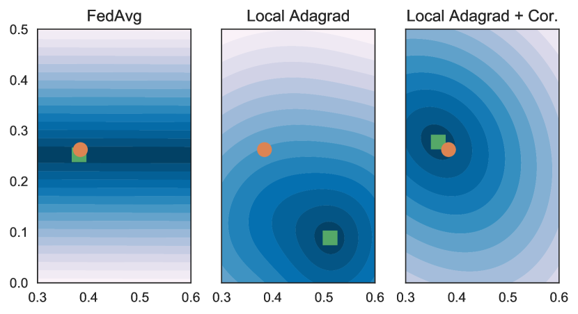
(a)

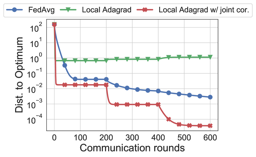
(b)

Figure 1: The effects of local adaptive methods on a synthetic 2D quadratic problem. Instantiations of FedOpt with local adaptivity can be viewed as finding the fixed points of some operator ${\mathbb{E}}[\mathcal{A}]$. For various methods, we plot (a) the norm $\|\bm{x}-{\mathbb{E}}[\mathcal{A}(\bm{x})]\|$, where darker colors indicate closer to the fixed point (Under local AdaGrad, the optimization landscape is better conditioned, but the fixed-point is inconsistent with the global minimum of the original global objective.); (b) training curves where the client learning rate is decayed at rounds $200,400$. We develop correction methods that can correct the inconsistency, while retaining the better conditioning.

Despite the success of using server-side adaptive methods, the power of adaptivity has not been fully utilized in the FedOpt framework, particularly on the client side. Instead of using adaptive methods only in ServerOpt for periodical updates per communication round, one can also choose to use adaptive methods in ClientOpt for every local iteration, or in both ClientOpt and ServerOpt. Client adaptive methods can accelerate the local convergence by better utilizing the geometric information of the local objectives. Unfortuantely, there are little to no literature exploring this promising direction. It remains an open problem whether the faster local convergence can be translated into faster global convergence and savings in communication rounds.

In this paper, we explore the usage of local adaptive methods and provide affirmative answers to the question: Can federated learning effectively use adaptive optimization methods on local clients? Specifically, our main contributions are listed as follows.

1. We identify that naively changing ClientOpt in the FedOpt framework from SGD to adaptive methods or other stateful optimizers can be problematic, as it does not define how to update client optimizer states (i.e., pre-conditioners and momentum buffers) across rounds. We propose to overcome this discontinuity issue by restarting the update of client optimizer states at the beginning of each round. This simple method enables the usage of local adaptivity in FedOpt. We also show that, on many practical training tasks, using adaptive optimizers on clients can achieve faster convergence and higher test accuracy than previous methods. color=blue!25, inline] Zheng: The previous sentence seems to be a bit vague and the logic on how it connects to the first sentence is not quite clear to me. What is the proposed method, and how did it overcome the issue described in the first sentence? Maybe just merge the two, drop the "identified" claim, and just directly describe we have a method to overcome the challenge. color=yellow!25, inline] Jianyu: Rephrase the complete part.

2. We further provide a theoretical analysis for strongly convex functions to understand the effects of various client optimizers. Our theorem suggests that performing FedOpt can be viewed as finding the fixed points of some operator ${\mathbb{E}}[\mathcal{A}]$, the expression of which is determined by client optimizers. Local adaptivity can change ${\mathbb{E}}[\mathcal{A}]$ in a way that yields faster convergence. However, this enhanced optimization may come with the cost of a non-vanishing solution bias – the point we converge to may be far away from the global minimizer of the original objective function, as illustrated in Figure 1.

3. In order to overcome the side effects of using adaptive client optimizers, we propose (1) local correction technique that can help to mitigate the non-vanishing solution bias; (2) global correction technique that can help to perserve the fast convergence property of adaptive methods. Using one or both of them on the top of adaptive client optimizers can achieve the highest test accuracy on all considered federated training tasks.

Related Works. In terms of using adaptive methods on clients, Xie et al. [16], Karimireddy et al. [17] proposed to use the same optimizer states (pre-conditioners and momentum buffers) on all clients, which is similar to server adaptive methods in [6] and does not exploit local adaptivity. To the best of our knowledge, this paper is the first to let clients separately update their optimizer states and study the effects of adaptive client optimizers. Besides, there are few recent literature [18, 19, 20, 21] also study the phenomenon that FedAvg-style algorithms can converge to a mismatched solution from the optimal one. We refer readers to Section 4 for detailed comparisons with these works. At last, within the FedOpt framework, there are many more building blocks that can accelerate the convergence or improve the practical performance, for instance, using control variates [22, 17, 23], regularizing the local objective functions [24, 25, 26], sampling important clients more frequently [27, 28, 29]. In this paper, we focus on an important but rarely studied topic – local adaptivity, which is orthogonal and complementary to the above previous works. color=blue!25, inline] Zheng: optional: I am not sure if claiming complementary is good enough or we want to be stronger on the difference, e.g., we care more of a cross-device settings with stateless clients. A reviewer may still ask us to compare with one of these methods. If we make the claim of the first sentence “There are extensive literature on accelerating the convergence of federated learning algorithms beyond the FedOpt framework” (which is arguable and assumes strong context of readers to know very nuanced parts of what belongs to FedOpt), we should have a strong support for why we limit ourselves to FedOpt. color=yellow!25, inline] Jianyu: I rewrote the above sentences. PTAL. Start with the local adaptivity. Add one more sentence.

2 Preliminaries

The Federated Learning Setup. In federated learning, the goal is to minimize the objective

$$F(\bm{x})={\mathbb{E}}_{i\sim\mathcal{C}}[F_{i}(\bm{x})]$$ (1)

where $F_{i}(\bm{x})=\frac{1}{|\mathcal{D}_{i}|}\sum_{\xi\in\mathcal{D}_{i}}f_{i}(\bm{x},\xi)$ denotes the local objective function at client $i$, and $f_{i}(\bm{x},\xi)$ is the loss function where $\xi$ represents one data sample from the local dataset. In contrast to classic distributed learning, federated learning does not allow clients to share their local data with others or with the central server. As a consequence, the local data distributions $\mathcal{D}_{i}$ may differ across clients. The term $\mathcal{C}$ denotes the distribution over the collection of all clients. The probability of selecting client $i$ is $w_{i}=\mathbb{P}_{\mathcal{C}}(i)$, which is proportional to the dataset size of client $i$. Thus, for a finite set of $M$ clients, the objective function becomes $F(\bm{x})=\sum_{i=1}^{M}w_{i}F_{i}(\bm{x})$.

Operator View of Client Optimizers. In this paper, we are going to use operators to represent the general optimizers on clients. In particular, for each client $i$, we have the following definition.

Definition 1 (Client Optimizer Operator).

We define an operator $\mathcal{A}_{i}(\bm{x};k,\Xi_{i},\bm{s}_{i}):\mathbb{R}^{d}\rightarrow\mathbb{R}^{d}$, which outputs the updated model after performing $k$ steps of a given client optimizer on the local objective $F_{i}$, from initial model $\bm{x}$, with initial optimizer states $\bm{s}_{i}$ and random sources $\Xi_{i}$ (e.g., noise in stochastic gradients).

The operator $\mathcal{A}_{i}$ defines how the local models and the client optimizer states (i.e., pre-conditioners and momentum buffers) are updated. When the parameters $k,\bm{s}_{i},\Xi_{i}$ are given, the output of $\mathcal{A}_{i}$ will only depend on the starting point $\bm{x}$. The specific form of $\mathcal{A}_{i}$ changes with the choice of optimizers and its analytical expression can be complicated. For example, when the client optimizer is pre-conditioned SGD (a generalized version of AdaGrad) [30], we have

$$\textstyle\mathcal{A}_{i}(\bm{x};k,\Xi_{i},\bm{s}_{i})=\bm{x}-\eta_{i}\sum_{s=0}^{k-1}\bm{P}_{i}^{(s)}g_{i}(\bm{x}^{(s)};\xi^{(s)})$$ (2)

where $\eta_{i}$ is the client learning rate, $\bm{x}^{(s)}$ is the local model after $s$ local iterations, $g(\bm{x}^{(s)};\xi^{(s)})$ denotes the stochastic gradient evaluated on a random mini-batch $\xi^{(s)}$, and $\bm{P}_{i}^{(s)}$ is referred to as the pre-conditioner. In vanilla SGD, the pre-conditioner is just the identity matrix; In AdaGrad, the pre-conditioner is updated as follows:

$$\bm{P}_{i}^{(s)}=((\bm{P}_{i}^{(s-1)})^{-2}+\operatorname{diag}\{g(\bm{x}^{(k)};\xi^{(k)})g(\bm{x}^{(k)};\xi^{(k)})^{\top}\})^{-\frac{1}{2}}$$ (3)

where $\bm{P}_{i}^{(-1)}=\bm{s}_{i}$ is the initial optimizer states. In this example, the random sources $\Xi_{i}=\{\xi^{(s)}\}$ represents all randomness in the stochastic gradients.

Operator View of FedOpt. Based on Definition 1, at each round $t$ of FedOpt, the server broadcasts the global model $\bm{x}^{(t)}$ as an initial point to clients. Then, client $i$ uses $\mathcal{A}_{i}$ to obtain the locally updated model as follows:

$$\bm{x}_{i}^{(t,\tau_{i})}=\mathcal{A}_{i}(\bm{x}^{(t)};\tau_{i},\Xi_{i}^{(t)},\bm{s}_{i}^{(t)}).$$ (4)

After that, the server aggregates local models changes $\bm{x}^{(t)}-\bm{x}_{i}^{(t,\tau_{i})}$ and uses ServerOpt to update the global model to $\bm{x}^{(t+1)}$. Since the server optimizer does not influence the properties of $\mathcal{A}_{i}$ and the main purpose of this paper is to understand the effects of client optimizers, we assume ServerOpt is gradient descent (GD) unless stated otherwise, which means that each client participates every round and there is no server pre-conditioner. Our results can be naturally extended to other server optimizers and sampled clients without changing the main insights on client optimizers. Then, the GD-based global update rule of FedOpt can be written as

$$\textstyle\bm{x}^{(t+1)}=\bm{x}^{(t)}-\alpha\sum_{i=1}^{M}w_{i}[\bm{x}^{(t)}-\mathcal{A}_{i}(\bm{x}^{(t)};\tau_{i},\Xi_{i}^{(t)},\bm{s}_{i}^{(t)})]$$ (5)

where $\alpha$ denotes the server learning rate for ServerOpt. color=blue!25, inline] Zheng: Maybe worth clarifying the difference compared to the original FedOpt? Did we generalize, or specify client optimizer? color=yellow!25, inline] Jianyu: This is just preliminary. So it is FedOpt itself without any generalizations. color=blue!25, inline] Zheng: I am not sure if $\Xi_{i}^{(t)},\bm{s}_{i}^{(t)}$ are part of FedOpt, it is more of "our interpretation" of FedOpt. color=yellow!25, inline] Jianyu: At least, $\Xi_{i}$ should be in the FedOpt algorithm, as it corresponds to the noise in stochastic gradients.

3 How to Apply Adaptive Methods on Clients

In this section, we describe the challenges of using local adaptivity in FedOpt and propose a simple, yet effective method to enable the usage of local adaptivity in FedOpt without incurring additional communication costs.

Challenge in FedOpt: Discontinuity of Client Optimizer States. According to the update rules 4 and 5 of FedOpt, we observe that FedOpt can not be directly applied to adaptive client optimizers, as it lacks the articulation of handling the initial optimizer states $\bm{s}_{i}$ across rounds and clients. To be specific, in FedOpt, the client updates are isolated not only from each other but also from different rounds due to the local iterations. While FedOpt uses ServerOpt to bridge the gap between local iterates in different rounds (i.e., it specifies how to obtain $\bm{x}^{(t+1)}$ from $\{\bm{x}_{i}^{(t,\tau_{i})}\}$), it does not define how to update the initial optimizer states $\bm{s}_{i}$ across rounds. We refer to this problem as discontinuity of client optimizer states.

A natural but impractical idea to tackle the discontinuity problem is to let each client inherit its own client optimizer states from previous rounds. However, these previous states can be stale and inaccurate because they are evaluated at point $\bm{x}_{i}^{(t-1,\tau_{i})}$ and do not take account of the possibly dramatic changes from $\bm{x}_{i}^{(t-1,\tau_{i})}$ to the current iterate $\bm{x}^{(t)}$. When the server only selects a random subset of clients at each round, the staleness will be further exacerbated, as one client may be disconnected from the server for multiple rounds. Besides, this solution is impossible in many applications of FL (e.g., the cross-device setting) that requires clients to be stateless and not to maintain any persistent states across rounds, due to privacy and system constraints [1]. Furthermore, one can also choose to synchronize the local optimizer states at the end of each round and use the synchronized states as the initial value for next round. For example, Yu et al. [31] has used a similar strategy to synchronize momentum buffer when the clients use momentum SGD. However, in order to aggregate and broadcast the additional optimizer states, this strategy would incur doubled or tripled communication costs compared to FedOpt with vanilla SGD client optimizer.

Our Proposal: Restarting Client Optimizer States. To work with the above challenges, we propose a simple yet effective approach. Instead of applying potentially complicated mechanisms to synchronize optimizer states across clients, we restart the updates of client optimizer states at the beginning of each round. That is, resetting the pre-conditioners to a constant and resetting the momentum buffers to zero. This strategy does not require any information from previous rounds, so it is compatible with application settings that require stateless clients. Also, it does not incur addition communication costs, as only the local model changes are aggregated.

To verify the advantage of this simple strategy, in Figure 1(b), we provide simulation results on a toy problem of quadratic functions with deterministic gradients. The result shows the restarting strategy on local AdaGrad (i.e., the green curve) can achieve significantly faster convergence speed, comparing to vanilla FedAvg (i.e., the blue curve) when the tolerance to the global optimal is relatively large. The fast convergence is also observed on practical federated training tasks (see Figure 2 and more discussions in Section 6).

4 Effects of Client Optimizers on Convergence and Consistency

Another important observation from the toy example in Figure 1(b) is that local AdaGrad converges to a point which is quite far away from the global optimum. Even if we decay the client learning rate, this inconsistency problem still cannot be mitigated or becomes even worse. In this section, we will theoretically analyze the effect of client optimizers on the convergence and provide insights into the trade-off between convergence speed and the consistency of the solution.

FedOpt Performs Fixed Point Iteration. When using the restarting strategy proposed in Section 3, the argument $\bm{s}_{i}$ representing the initial optimizer state in the operator $\mathcal{A}_{i}$ can be omitted since it is set to its default initial value and is the same on all clients. We further define an operator $\mathcal{A}(\bm{x})=\sum_{i=1}^{M}w_{i}\mathcal{A}_{i}(\bm{x};\tau_{i},\Xi_{i})$. Accordingly, the global update rule (see Eqn. 5) of FedOpt is equivalent to a stochastic fixed point iteration, shown as follows:

$$\bm{x}^{(t+1)}=(1-\alpha)\bm{x}^{(t)}+\alpha{\mathbb{E}}[\mathcal{A}(\bm{x}^{(t)})]+\alpha(\mathcal{A}(\bm{x}^{(t)})-{\mathbb{E}}[\mathcal{A}(\bm{x}^{(t)})])$$ (6)

where $\alpha$ denotes the server learning rate and the expectation is taken over all random sources in local stochastic gradients at the current round. The deterministic version of 6 is known as Mann’s iteration [32] and will converge to the fixed points of ${\mathbb{E}}[\mathcal{A}]$ under certain conditions. Replacing server GD with another server optimizer can accelerate the convergence but it will not influence the properties and the fixed points of the operator ${\mathbb{E}}[\mathcal{A}]$.

We will analyze the convergence of FedOpt (update rule of which is 6) in the setting where each local objective function $F_{i}(\bm{x})$ is $L_{i}$-Lipschitz smooth and $\mu_{i}$-strongly convex. Besides, we make the following assumptions on the properties of each client optimizer $\mathcal{A}_{i}$ and show how the global convergence is influenced by these properties. If the client optimizer is SGD, then the contractive local operator and bounded cumulative variance properties described below follow directly from the strong convexity and smoothness of the objective function, suggesting the following assumptions are reasonable and mild.

Assumption 1 (Contractive Local Operator).

The local expected operator ${\mathbb{E}}[\mathcal{A}_{i}]$ is contractive, satisfying that $\left\|{\mathbb{E}}[\mathcal{A}_{i}(\bm{x};k,\Xi)]-{\mathbb{E}}[\mathcal{A}_{i}(\bm{y};k,\Xi)]\right\|^{2}\leq h_{i}(k)\cdot\left\|\bm{x}-\bm{y}\right\|^{2}$ for any $\bm{x},\bm{y}\in\mathbb{R}^{d}$, where $0<h_{i}(k)<1$ is a decreasing function of the number of local steps $k$.

Assumption 2 (Bounded Cumulative Variance).

We assume the local stochastic gradient $g_{i}$ is an unbiased estimator of $\nabla F_{i}$ and has bounded variance: ${\mathbb{E}}\left\|g_{i}(\bm{x})-\nabla F_{i}(\bm{x})\right\|^{2}\leq\sigma^{2}$. Similarly, the local operator $\mathcal{A}_{i}$ has bounded cumulative variance: ${\mathbb{E}}\left\|\mathcal{A}_{i}(\bm{x};k,\Xi)-{\mathbb{E}}[\mathcal{A}_{i}(\bm{x};k,\Xi)]\right\|^{2}\leq q_{i}(k)\cdot\sigma^{2}$, where $q_{i}(k)>0$ is a non-decreasing function of the number of local steps $k$.

The function $h_{i}(k)$ in Assumption 1 measures the local training progress of ClientOpt. In intuition, when ClientOpt has faster convergence rate or takes more local steps, the output of ${\mathbb{E}}[\mathcal{A}_{i}]$ will be closer to the minimum $\bm{x}_{i}^{*}$, and hence $h_{i}$ will become smaller. Besides, the function $q_{i}(k)$ in Assumption 2 quantifies how the noise in stochastic gradients are accumulated through $k$ local updates. The analytical forms of $h_{i},q_{i}$ depend on the choice of ClientOpt. For example, when the client optimizer is SGD with fixed client learning rate, we formally prove in Appendix B that $h_{i}(k)=(1-\eta_{i}\mu_{i})^{2k}$ and $q_{i}(k)=\eta_{i}^{2}k$. For adaptive optimizers, such as AdaGrad and Adam, while it is difficult to obtain the analytical form of $h_{i}$, we empirically validate Assumption 1 in Section B.4 and found they can yield smaller $h_{i}$ values than vanilla SGD.

Theorem 1 (Convergence of FedOpt and Minimizer Inconsistency).

Under Assumptions 1 and 2, the operator ${\mathbb{E}}[\mathcal{A}]$ is contractive and has a unique fixed point $\widetilde{\bm{x}}$. After total $T$ communication rounds, the global iterates of FedOpt converge to $\widetilde{\bm{x}}$ at the following rate for some positive constant $c$:

$${\mathbb{E}}\|\bm{x}^{(T)}-\widetilde{\bm{x}}\|^{2}\leq c\cdot\left(\left[\sum_{i=1}^{M}w_{i}h_{i}\right]^{T}\frac{\|\bm{x}^{(0)}-\widetilde{\bm{x}}\|^{2}}{1-\sum_{i=1}^{M}w_{i}h_{i}}+\frac{1}{T}\frac{\sigma^{2}\sum_{i=1}^{M}w_{i}^{2}q_{i}}{(1-\sum_{i=1}^{M}w_{i}h_{i})^{2}}\right).$$ (7)

In the presence of data heterogeneity, the fixed point $\widetilde{\bm{x}}$ of ${\mathbb{E}}[\mathcal{A}]$ is not necessarily the same as the optimum $\bm{x}^{*}$ of the global objective $F$. We refer to this problem as minimizer inconsistency.

Better Client Optimizers Can Accelerate the Global Convergence. Theorem 1 provides a nice connection between local and global convergence. Specifically, if clients use better client optimizers that have smaller contraction constant $h_{i}$, then the worst-case global convergence to the fixed point $\widetilde{\bm{x}}$ can be improved, as the error bound 7 monotonically increases with $h_{i}$. Therefore, a natural strategy to speedup the global convergence is to separately minimize $h_{i}$ on each client while keeping $q_{i}$ unchanged. One can achieve this by either tuning a proper learning rate for each client, or using adaptive client optimizers which could reduce the effective local condition number. Intuitively, using better client optimizers makes the operator ${\mathbb{E}}[\mathcal{A}]$ to be more contractive, and hence, it becomes easier to find its fixed points (as corroborated in Figure 1(a), the loss surface is better conditioned when using local AdaGrad). This acceleration effects is complementary to that of the server optimizer, which changes the form of the fixed point iteration without affecting ${\mathbb{E}}[\mathcal{A}]$. Therefore, one can use both better client and server optimizers to get the best performance, as we will later illustrate in Section 6.

The Minimizer Inconsistency Problem. Theorem 1 also shows that the speedup effects of client optimizers may come with a price: the fixed point $\widetilde{\bm{x}}$ can be different from the optimal minimizer $\bm{x}^{*}$. When the objective function is quadratic, ClientOpt is GD and all clients have the same learning rates $\eta$ and number of local steps $\tau$, it has been shown in [19, 20] that $\|\widetilde{\bm{x}}-\bm{x}^{*}\|=\mathcal{O}(\eta(\tau-1))$ such that one can balance the trade-off between convergence speed and the minimizer inconsistency by gradually decaying the client learning rate. However, through a simple counterexample below, we will show that using adaptive optimizers or different hyper-parameters on clients leads to an additional gap between $\widetilde{\bm{x}}$ and $\bm{x}^{*}$, which does not vanish to zero with the learning rate. This non-vanishing bias explains our empirical observations in Figure 1(b) and calls for new techniques to overcome it.

Quadratic Example for Theorem 1. In this toy example, we assume the loss function for client $i$ is given by $F_{i}(\bm{x})=\frac{1}{2}\bm{x}^{\top}\bm{H}_{i}\bm{x}-\bm{e}_{i}^{\top}\bm{x}+\bm{c}_{i}$, where $\bm{H}_{i}$ is symmetric and positive definite and $\bm{e}_{i},\bm{c}_{i}$ are some vectors. Accordingly, the minimum of $F_{i}$ is simply $\bm{x}^{*}_{i}=\bm{H}_{i}^{-1}\bm{e}_{i}$ and the minimum of the global objective is $\bm{x}^{*}=(\sum_{i=1}^{M}w_{i}\bm{H}_{i})^{-1}\sum_{i=1}^{M}w_{i}\bm{H}_{i}\bm{x}_{i}^{*}$.

Theorem 2.

For the quadratic problem, if the client optimizer is preconditioned GD with a fixed pre-conditioner $\bm{P}_{i}$, then $\widetilde{\bm{x}}=(\sum_{i=1}^{M}w_{i}[\bm{I}-\bm{K}_{i}])^{-1}\sum_{i=1}^{M}w_{i}[(\bm{I}-\bm{K}_{i})\bm{x}_{i}^{*}]\neq\bm{x}^{*}$, where $\bm{K}_{i}=(\bm{I}-\eta_{i}\bm{P}_{i}\bm{H}_{i})^{\tau_{i}}$. If we let $\eta_{i}=\gamma_{i}\eta$ and $\eta$ approach to zero, then it follows that

$$\textstyle\lim_{\eta\rightarrow 0}\widetilde{\bm{x}}=(\sum_{i=1}^{M}w_{i}\gamma_{i}\tau_{i}\bm{P}_{i}\bm{H}_{i})^{-1}(\sum_{i=1}^{M}w_{i}\gamma_{i}\tau_{i}\bm{P}_{i}\bm{H}_{i}\bm{x}_{i}^{*})\neq\bm{x}^{*}.$$ (8)

Theorem 2 shows that as long as one of the factors (i.e., client learning rate, the number of local steps, the pre-conditioners) is different across clients, then there would appear a non-vanishing gap between $\widetilde{\bm{x}}$ and $\bm{x}^{*}$. In order to get an intuition behind this phenomenon, we can check the exact expression of $\bm{x}^{*}-\mathcal{A}(\bm{x}^{*})$. If $\widetilde{\bm{x}}=\bm{x}^{*}$, then $\bm{x}^{*}-\mathcal{A}(\bm{x}^{*})$ should always be zero. However, note that

$$\textstyle{\bm{x}^{*}-\mathcal{A}(\bm{x}^{*})=\sum_{i=1}^{M}w_{i}[\bm{I}-(\bm{I}-\eta_{i}\bm{P}_{i}\bm{H}_{i})^{\tau_{i}}]\bm{H}_{i}^{-1}\nabla F_{i}(\bm{x}^{*}).}$$ (9)

In Eqn. 9, each local objective’s gradient is implicitly weighted by a matrix $\bm{M}_{i}=[\bm{I}-(\bm{I}-\eta_{i}\bm{P}_{i}\bm{H}_{i})^{\tau_{i}}]\bm{H}_{i}^{-1}$. The aggregated local changes $\bm{x}^{*}-\mathcal{A}(\bm{x}^{*})=\sum_{i=1}^{M}w_{i}\bm{M}_{i}\nabla F_{i}(\bm{x}^{*})$ can be consisdered as a skewed version of the global gradient $\nabla F(\bm{x}^{*})=\sum_{i=1}^{M}w_{i}\nabla F_{i}(\bm{x}^{*})=0$. Only if $\bm{M}_{i}=\bm{M}_{j}$ for all client pairs $i,j$, we can conclude that $\bm{x}^{*}=\mathcal{A}(\bm{x}^{*})$ and hence $\widetilde{\bm{x}}=\bm{x}^{*}$. However, due to the data heterogeneity, the condition $\bm{M}_{i}=\bm{M}_{j}$ does not hold. Furthermore, if we omit higher order terms $\eta_{i}^{2}$ in 9, then we get the following via Taylor approximation:

$$\textstyle[\bm{x}^{*}-\mathcal{A}(\bm{x}^{*})]/(\max_{i}\eta_{i}\tau_{i})=\sum_{i=1}^{M}w_{i}\frac{\eta_{i}\tau_{i}\bm{P}_{i}}{\max_{i}\eta_{i}\tau_{i}}\nabla F_{i}(\bm{x}^{*})+\mathcal{O}(\eta_{i}\tau_{i})$$ (10)

where the first term (on the right hand side) corresponds to the non-vanishing gap between $\widetilde{\bm{x}}$ and $\bm{x}^{*}$, and the second term can be omitted when the client learning rate is sufficiently small. It is worth noting that if $\eta_{i}=0$ or $\tau_{i}=0$, then $\bm{x}=\mathcal{A}(\bm{x})$ for any $\bm{x}\in\mathbb{R}^{d}$, as there is no optimization progress at all. Therefore, in order to exclude this invalid solution, we divide $(\max_{i}\eta_{i}\tau_{i})$ in 10.

This toy example also illustrates how local adaptivity can accelerate convergence. In particular, when the local pre-conditioners are ideal (i.e., inverse of local Hessians), FedOpt can converge to $\widetilde{\bm{x}}$ in just one round by choosing proper server and client learning rates. But if the local pre-conditioner are the same across all clients ($\bm{P}_{i}=\bm{P}$), then the convergence of FedOpt will depend on the condition numbers of $\{\bm{P}\bm{H}_{i}\}$ and require multiple rounds.

Connections with Previous Works on Minimizer Inconsistency. When client learning rates, number of local steps are the same across all clients, and non-adaptive, deterministic ClientOpt are used, $\|\widetilde{\bm{x}}-\bm{x}^{*}\|$ can vanish to zero along with the learning rates. This phenomenon has been observed and analyzed by few recent literature in different forms, see [19, 21, 20]. Theorem 1 generalizes these results by allowing heterogeneous local hyper-parameters and adaptive, stochastic client optimizers. In addition, the non-vanishing bias was studied in [18] by assuming different local learning rates and local steps at clients. In this paper, we further generalize the results by showing that even when the learning rates and local steps are the same, using local adaptive methods will lead to a non-vanishing gap. We summarize the differences in Table 6 of Appendix D.

5 Correction Techniques to Overcome the Non-vanishing Solution Bias

As we discussed in Section 4, while using faster client optimizers and exploiting local structures can help improve the global convergence, this strategy results in a non-vanishing gap between the converged point $\widetilde{\bm{x}}$ and the optimal solution $\bm{x}^{*}$. Inspired by the quadratic example in Section 4, we propose (i) a local correction method that reweights local gradients before sending the client updates to the server in order to overcome the non-vanishing part of minimizer inconsistency, and (ii) a global correction method applied by the server when aggregating the client updates in order to preserve fast convergence.

Local Correction: Reweighting Local Gradients. From 10 in the quadratic example, one can observe that the non-vanishing minimizer inconsistency comes from the fact that FedOpt implicitly and improperly weights each local gradients by a matrix $\bm{N}_{i}=\eta_{i}\tau_{i}\bm{P}_{i}$. So a natural solution to overcome the non-vanishing bias is to normalize the local model changes before aggregating them on the server. Instead of sending $\bm{x}-\mathcal{A}_{i}(\bm{x})=\bm{N}_{i}\nabla F_{i}(\bm{x})+\mathcal{O}(\eta_{i}^{2})$ to the server, each client can send the locally normalized version $\bm{N}_{i}^{-1}(\bm{x}-\mathcal{A}_{i}(\bm{x}))$. This simple change can ensure that the first term in 10 is always zero no matter which value is the client learning rate. As a consequence, there is no non-vanishing solution bias. The local correction technique also automatically avoids the invalid solution $\bm{x}=\mathcal{A}(\bm{x}),\forall\bm{x}$ by dividing the client learning rate.

The local correction technique can be extended to more general settings and work with any adaptive optimizers, such as AdaGrad, Adam. If the local model changes of a specific client optimizer can be written as $\bm{x}-\mathcal{A}_{i}(\bm{x};\tau_{i})=\eta_{i}\sum_{k=0}^{\tau_{i}-1}\bm{B}_{i}^{(k)}\nabla F_{i}(\bm{x}^{(k)})$ where $\bm{B}_{i}^{(k)}$ is symmetric and positive-definite and $\bm{x}^{(k)}$ denotes the $k$-th iterate during local updates, then we can choose the local correction matrix to be $\bm{N}_{i}=\eta_{i}\sum_{k=0}^{\tau_{i}-1}\bm{B}_{i}^{(k)}$ such that

$$\textstyle\sum_{i=1}^{M}w_{i}\bm{N}_{i}^{-1}(\bm{x}^{*}-\mathcal{A}_{i}(\bm{x}^{*}))=\underbrace{\textstyle{\sum_{i=1}^{M}}w_{i}\nabla F_{i}(\bm{x}^{*})}_{=\nabla F(\bm{x}^{*})=0}+\mathcal{O}(\eta_{i}\tau_{i})=\mathcal{O}(\eta_{i}\tau_{i}).$$ (11)

If the client optimizer is AdaGrad, then $\bm{B}_{i}^{(k)}$ is just the pre-conditioner $\bm{P}_{i}^{(k)}$ used at the $k$-th local iteration; if the client optimizer is Adam, then $\bm{B}_{i}^{(k)}$ is a weighted summation of local pre-conditioners. In Section A.3, we provide the pseudo-code of finding the expression of $\bm{N}_{i}$ for common optimizers; and in Appendix F, we formally prove that local correction can help FedOpt with deterministic client optimizers converge to the stationary points of the original objective function (even when it is non-convex). For stochastic client optimizers, we empirically validate the effectiveness of local correction through extensive experiments in Section 6.

Global Correction: Preserving the Fast Convergence. Equation 11 shows that using the local correction technique may change the scale of the aggregated model updates. In particular, the first-order approximation of the aggregated model updates just equals to plain gradients (the first term in 11) and may lose the local pre-conditioning effects. In order to address this problem, one can use either adaptive server optimizer that are more robust to the scale of its inputs, or a novel global correction technique that can help to preserve the scale of local updates. To be specific, in global correction, the server uses $\bm{N}_{s}^{-1}\sum_{i=1}^{M}w_{i}\bm{N}_{i}^{-1}[\bm{x}-\mathcal{A}_{i}(\bm{x})]$ as the pseudo-gradient of ServerOpt, where $\bm{N}_{s}$ is given as $\bm{N}_{s}=\sum_{i=1}^{M}w_{i}\bm{N}_{i}^{-1}$. There may also exist other better choices of the matrix $\bm{N}_{s}$. As long as $\bm{N}_{s}$ does not depend on the client index $i$, it will not influence the fixed point, to which the algorithm converge. We name this technique as global correction, because it is applied on the server side. In order to obtain $\bm{N}_{s}$, the clients need to send the local correction matrices $\bm{N}_{i}$ to the server. But the server does not need to broadcast the correction matrix $\bm{N}_{s}$ back. Therefore, if matrices $\{\bm{N}_{i}\}$ are diagonal, then the communication cost per round of using global correction is only $1.5\times$ than that of without using it. color=blue!25, inline] Zheng: We should probably have one sentence talking about algorithm 1 somewhere.

6 Experiments

In this section, we summarize the experimental results and validate the effectiveness of the proposed methods. Specifically, we show that FedOpt with local adaptivity and correction techqniues can achieve faster convergence, higher test accuracy, as well as more robustness against learning rate changes than previous server-only adaptive methods.

We focus on three language-related tasks [6], which have the favored sparse structures for adaptive methods: (i) Next word prediciton using RNN on Stack Overflow (SO NWP); (ii) next character prediction using RNN on Shakespeare (Shakes. NCP); (iii) tag prediction using linear regression on Stack Overflow (SO TP). For the first two tasks, we report the validation/test accuracy. For SO TP task, we report the validation/test Recall@5. Moreover, we also evaluate the methods in image classification task on the CIFAR100 dataset [33]. The detailed descriptions (hyper-parameter tuning ranges and choices) of these federated training tasks are provided in Appendix A. Our implementation based on the Tensorflow Federated (TFF) package will be open-sourced.

Faster Convergence. In Figure 2, we first compare the training curves of different ways of using AdaGrad in FedOpt on the SO NWP training task. One can either use AdaGrad on clients, or on the server, or on both. It can be observed that using local AdaGrad can significantly speedup the convergence compared to using vanilla SGD as the client optimizer. In particular, client-only AdaGrad is even slightly faster than server-only AdaGrad. When the local epoch increases from $1$ to $5$, the improvement of client-only AdaGrad over server-only AdaGrad becomes more obvious. If we apply AdaGrad on both clients and the server, then FedOpt achieves the fastest convergence (about $4\times$ faster than server-only AdaGrad to achieve $20\%$ validation accuracy in Figure 2a).

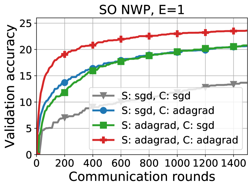
(a)

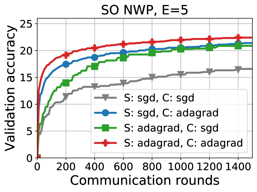
(b)

Figure 2: Example of training curves of FedOpt variants on the SO NWP task. The adaptive client optimizer is used with the proposed restarting strategy. In the legend, “C” and “S” denote the ClientOpt and the ServerOpt, respectively. Using AdaGrad on both clients and server is significantly faster than other variants.

Higher Final Accuracy. We further report the test accuracy or Recall@5 on different training tasks in Table 1. Similar to the above discussions on faster convergence, changing ClientOpt from SGD to AdaGrad and using the restarting strategy prposed in section 3 consistently improves the test accuracy on multiple training tasks. And applying AdaGrad on both clients and the server achieves the highest test accuracy. For example, when the ServerOpt is AdaGrad, the test accuracy improves from $21.80\%$ to $24.40\%$ on SO NWP, and from $57.68\%$ to $57.85\%$ on Shakes. NCP. However, note that on the SO TP task, server AdaGrad plus client AdaGrad with the restarting strategy performs worse than server-only AdaGrad ($65.79$ versus $66.39$). This performance degradation may come from the non-vanishing solution bias, as we discussed in Section 4.

	C:SGD	C:AdaGrad
S:SGD	14.19	21.68
S:AdaGrad	21.80	24.40

(a) SO NWP

C:SGD	C:AdaGrad
57.12	57.47
57.68	57.85

(b) Shakes. NCP

C:SGD	C:AdaGrad
34.50	39.67
66.39	65.79

(c) SO TP

Table 1: The test accuracy ($\%$) and recall@5 ($\times 100$) after $1500$ communication rounds of FedOpt variants on different training tasks. Darker color means better performance.

Training Tasks	ServerOpt	ClientOpt
		SGD	AdaGrad	+ Local Cor.	+ Joint Cor.
SO NWP	Adam	$24.40$	$24.70$	$24.81$	$\mathbf{24.85}$
Shakes. NCP	AdaGrad	$57.68$	$57.85$	$57.75$	$\mathbf{58.06}$
SO TP	AdaGrad	$66.39$	$65.79$	$\mathbf{67.04}$	$66.94$

Table 2: Comparison of our proposed methods (column 2,3,4) and the best server-only adaptive methods (column 1) for each training task. The table shows the test accuracy ($\%$) or recall@5 ($\times 100$) after $1500$ communication rounds. Bolded ones are the best results for each training tasks. In the table, we fix $\epsilon=10^{-7}$ in ClientOpt and tune $\epsilon_{s}$ in ServerOpt. Therefore, the performance of our proposed methods (column 2,3,4) can be further improved by tuning the $\epsilon$ parameter.

Then, we evaluate the proposed correction techniques in Table 2 and compare the results with the best server-only adaptive methods on each training tasks (the best server optimizer is selected based on the results in [6]). On SO TP, by overcoming the non-vanishing bias, client AdaGrad with local correction can achieve much higher Recall@5 than vanilla SGD optimizer ($67.04$ versus $66.39$). Similar improvements also appear in SO NWP and Shakes. NCP tasks. Besides client AdaGrad, our proposed methods also work for other common momentum-based adaptive optimizers (such as Adam and Yogi [13]). We present the experimental results on SO NWP in Table 3. It can be observed that our proposed method relatively improves the test accuracy of server Adam plus client SGD by $3.9\%$ ($25.35\%$ versus $24.40\%$), and vanilla FedAvg by $78.6\%$ ($25.35\%$ versus $14.19\%$).

ClientOpt	No Cor.	Local Cor.	Joint Cor.
Yogi [13]	$24.80$	$25.29$	25.33
Adam	$24.86$	$25.15$	25.35

Table 3: Performance (test accuracy ($\%$) after $1500$ rounds of training) of momentum-based adaptive client optimizers on SO NWP. The ServerOpt is fixed as Adam. Recall that the test accuracy of sever Adam plus client SGD is $24.40\%$.

Less Sensitive to Hyper-parameter Changes. In Figure 3, we report how the test accuracy changes with server and client learning rates on the SO NWP task. We observe that for server-only AdaGrad, there is only two out of $28$ learning rate combinations that can achieve a $20\%+$ test accuracy. On the other hand, using AdaGrad on both clients and server are more robust to the learning rate changes. There are $10$ out of $28$ combinations reaching a $20\%+$ test accuracy. The less sensitivity to learning rate changes can help people to save hyper-parameter tuning time in practice.

(a) S: AdaGrad, C: AdaGrad

(b) S: AdaGrad, C: SGD

Figure 3: How the test accuracy changes with server and client learning rate in FedOpt. Using local adaptive methods make the algorithm be more robust to the hyper-parameter changes.

Comparison with the Synchronizing States Strategy. We further compare the proposed restarting optimizer states strategy to a synchronizing strategy where local pre-conditioners are synchronized after each round. Surprisingly, the additional communication in the synchronized strategy does not help and achieves even worse accuracy. For instance, on Shakes. NCP, server AdaGrad plus synchronized client AdaGrad has a test accuracy of $56.89\%$, which is lower than that of the restarting one ($57.85\%$).

Results on Image Classification Task. At last, we examine the performance of the proposed methods on pathological version of CIFAR100, following the setup in [6]. The observations are similar to language related tasks. Naively using client adaptive methods in FedOpt is not guaranteed to have better performance. But when combining local adaptvity with the proposed correction techniques, the performance consistently improves. Specifically, after $8000$ communication rounds, while server Adam plus client AdaGrad has worse test accuracy than server-only Adam ($54.68\%$ vs $56.64\%$), using local correction can improve the accuracy to $56.80\%$.

7 Conclusions

In this paper, we first propose techniques that enable the use of adaptive optimization methods for local updates at clients in federated learning. Through the analysis on effects of client optimizers for smooth and strongly convex functions, we show that although local adaptive methods can accelerate the convergence in some scenarios, it introduces an additional non-vanishing gap between the converged point and the optimal solution. To mitigate the side effects of using local adaptivity, we further propose local and global correction techniques. We verified the advantages of the proposed methods regarding fast convergence, better test accuracy with extensive experiments on benchmark datasets.

Appendix A Experimental Details

In this section, we describe our experimental setup in more detail. A brief summary of tunning ranges and default values for hyper-parameters are summarized in Table 4.

Tasks	SO NWP	Shakes. NCP	SO TP
Models	RNN	RNN	LR
Total number of clients	$342477$	$715$	$342477$
Maximal elements per client	$128$	N/A	$1000$
Active clients per round	$50$	$10$	$10$
Mini-batch size	$16$	$4$	$100$
Default Local epochs	$1$	$1$	$1$
Total rounds	$1500$	$1500$	$1500$
Client learning rate $\log_{10}(\eta)$	$\{-3,-2.5,\dots,-1,0,0.5\}$		$\{-1,-0.5,\dots,2,2.5\}$
Server learning rate $\log_{10}(\alpha)$	$\{-1.5,-1,-0.5,0,0.5,1\}$		$\{-0.5,0,0.5,1,1.5\}$
Parameter $\epsilon_{s}$ in ServerOpt	$\log_{10}(\epsilon_{s})=\{-7,-5,-3,-1\}$
Parameter $\epsilon$ in ClientOpt	$\log_{10}(\epsilon)=\{-7\}$

Table 4: Experimental settings, default values and tuning ranges of hyper-parameters.

A.1 Training Tasks

Next-Word Prediction on Stack Overflow (SO NWP for short).

Stack Overflow is a language modeling dataset from the question and answer site, Stack Overflow. The datasets consists of questions and answers from $342,477$ unique users, each of which is treated as a client in our experiments. We perform next-word prediction task on this dataset and restrict to the 10,000 most frequently used words. The preprocess procedure of this datasets follows [6]. Specifically, we let each client only use the first 128 sentences of its local dataset, in order to avoid that clients have extremely different amount of data. Padding and truncation are used to ensure that sentences have 20 words. The metrics we report are the top-1 validation and test accuracy over the $10,000$-word vocabulary. It does not include padding, out-of-vocab, or beginning or end or sentence tokens. The neural network model we use is a RNN with single LSTM layer, which is the same as that of [6].

Tag Prediction on Stack Overfolow (SO TP for short).

Tag prediction via logistic regression is another training task on the Stack Overflow datasets. It has the same number of clients and vocabulary size as SO NWP. Besides, following the setup in [6], we use the $500$ most frequent tags and a one-versus-rest classification strategy.

Next Character Prediction on Shakespeare (Shakes. NCP for short).

Shakespeare is another language modeling dataset built from the works from William Shakespeare. Each client corresponds to a speaking role with at least two lines. The lines of each speaking role is splitted into sequences of 80 characters, padding if necessary. The vocabulary size is 90. The neural networks model we use is the same as [6]: a RNN with two LSTM layers.

A.2 Best Performing Hyper-parameters

We report the best performed hyper-parameters in Table 5. The hyper-parameters are selected in a way such that the average validation accuracy (or recall@5) over the last $100$ rounds achieves the highest value.

Training Tasks	ServerOpt	ClientOpt
		SGD	AdaGrad	+ Local Cor.	+ Joint Cor.
SO NWP	SGD	$(-0.5,0,\text{NA})$	$(-0.5,0,\text{NA})$	$(0,0.5,\text{NA})$	$(-0.5,0,\text{NA})$
	AdaGrad	$(-0.5,-1.5,-3)$	$(-0.5,-1,-5)$	$(-0.5,-1,-5)$	$(-0.5,-1,-7)$
	Adam	$(-0.5,-1.5,-5)$	$(-0.5,-1.5,-3)$	$(-1,-1.5,-5)$	$(-1,-1.5,-5)$
Shakes. NCP	SGD	$(0,0,\text{NA})$	$(-0.5,-0.5,\text{NA})$	$(-0.5,2,\text{NA})$	$(-0.5,0,\text{NA})$
	AdaGrad	$(0.5,-1,-1)$	$(0,-1,-3)$	$(-0.5,-1,-5)$	$(-0.5,-0.5,-1)$
SO TP	SGD	$(2.5,0,\text{NA})$	$(1.5,0,\text{NA})$	$(1.5,1.5,\text{NA})$	$(1.5,0,\text{NA})$
	AdaGrad	$(0.5,1,-5)$	$(-0.5,1,-5)$	$(-0.5,1,-7)$	$(-0.5,1,-5)$
	Adam	$(1.5,-0.5,-5)$	$(1,-0.5,-5)$	$(0.5,-0.5,-7)$	$(1,-0.5,-5)$

Table 5: Best performed hyper-parameters in all training tasks. The tuple in each cell corresponds to $(\eta,\alpha,\epsilon_{s})$: client learning rate, server learning rate, and adaptivity parameter $\epsilon_{s}$ in the ServerOpt.

A.3 Pseudo-Codes of The Proposed Algorithms

We present the pseudo-codes for our proposed algorithms in Algorithm 1. It is worth noting that Algorithm 1 only provides a concrete specification of the proposed local and global correction techniques. Beyond our choices, there may exist many other algorithmic variants.

1:  Input: Initial model $\bm{x}^{(0)}$, ClientOpt, ServerOpt 2:  for $t\in\{0,1,\dots,T-1\}$  do 3:     for client $i$ in the random set $\mathcal{S}^{(t)}$ in parallel do 4:        Initialization $\bm{x}_{i}^{(t,0)}=\bm{x}^{(t)}$, $\bm{m}_{i}^{(t,-1)}=0,\bm{P}_{i}^{(t,-1)}=c$, $\bm{N}_{i}^{(t)}=0,\bm{M}_{i}^{(t,-1)}=0$ 5:        for $k\in\{0,\dots,\tau_{i}-1\}$ do 6:           Compute local stochastic gradient $g_{i}(\bm{x}_{i}^{(t,k)})$ and update local pre-conditioner $\bm{P}_{i}^{(t,k)}$ 7:           Update momentum $\bm{m}_{i}^{(t,k)}=\beta_{1}\bm{m}_{i}^{(t,k-1)}+(1-\beta_{1})g_{i}(\bm{x}_{i}^{(t,k)})$ 8:           Update local model $\bm{x}_{i}^{(t,k+1)}=\bm{x}_{i}^{(t,k)}-\eta\bm{P}_{i}^{(t,k)}\bm{m}_{i}^{(t,k)}$ 9:           $\bm{M}_{i}^{(t,k)}=\beta_{1}\bm{M}_{i}^{(t,k-1)}+(1-\beta_{1})\bm{P}_{i}^{(t,k)}$ 10:           $\bm{N}_{i}^{(t)}\leftarrow\bm{N}_{i}^{(t)}+\bm{M}_{i}^{(t,k)}$ 11:        end for 12:        Local changes $\Delta_{i}^{(t)}=\bm{x}^{(t)}-\bm{x}_{i}^{(t,\tau_{i})}$ 13:        $\Delta_{i}^{(t)}\leftarrow(\bm{N}_{i}^{(t)})^{-1}\Delta_{i}^{(t)}$ 14:     end for 15:     Aggregate $\Delta^{(t)}=\frac{1}{|\mathcal{S}^{(t)}|}\sum_{i\in\mathcal{S}^{(t)}}\Delta_{i}^{(t)}$ 16:     Aggregate $\bm{N}_{s}^{(t)}=\frac{1}{|\mathcal{S}^{(t)}|}\sum_{i\in\mathcal{S}^{(t)}}(\bm{N}_{i}^{(t)})^{-1}$ and set $\Delta^{(t)}\leftarrow(\bm{N}_{s}^{(t)})^{-1}\Delta^{(t)}$ 17:     $\bm{x}^{(t+1)}=\textsc{{ServerOpt}}(\bm{x}^{(t)},\Delta^{(t)},\alpha,t)$ 18:  end for

Algorithm 1 Local adaptive FedOpt with the restarting strategy and local correction, global correction techniques

Appendix B Justifications of Assumptions 1 and 2 for Vanilla SGD Client Optimizer

B.1 Two Useful Lemmas

Before we dive into the proofs, we would like to first introduce two useful lemmas, which will be repeatedly applied later on.

Lemma 1.

Suppose function $F$ is twice-differentiable. Then, for any points $\bm{x},\bm{y}\in\mathbb{R}^{d}$, we have

$$\nabla F(\bm{x})-\nabla F(\bm{y})=\bm{H}(\bm{x}-\bm{y})$$ (12)

where $\bm{H}=\int_{0}^{1}\nabla^{2}F(\bm{y}+s(\bm{x}-\bm{y}))\mathrm{d}s$.

Proof.

Due to the linearity of integral, we have

$$\nabla F(\bm{x})-\nabla F(\bm{y})=\int_{0}^{1}\nabla^{2}F(\bm{y}+s(\bm{x}-\bm{y}))(\bm{x}-\bm{y})\mathrm{d}s=\bm{H}(\bm{x}-\bm{y}).$$ (13)

∎

Lemma 2.

Suppose $\bm{x}$ and $\bm{y}$ are random variables with the same random sources $\xi$. Then, if a function $F$ is $L$-lipschitz smooth and $\mu$-strongly convex, then we have

$$\left\|{\mathbb{E}}[\nabla F(\bm{x})-\nabla F(\bm{y})]\right\|^{2}\geq \mu^{2}\left\|{\mathbb{E}}[\bm{x}-\bm{y}]\right\|^{2}$$ (14)

$$\left\|{\mathbb{E}}[\nabla F(\bm{x})-\nabla F(\bm{y})]\right\|^{2}\leq L\left<{{\mathbb{E}}[\bm{x}-\bm{y}]},\,{{\mathbb{E}}[\nabla F(\bm{x})-\nabla F(\bm{y})]}\right>$$ (15)

$$(\mu+L)\left<{{\mathbb{E}}[\nabla F(\bm{x})-\nabla F(\bm{y})]},\,{{\mathbb{E}}[(\bm{x}-\bm{y})]}\right>\geq \left\|{\mathbb{E}}[\nabla F(\bm{x})-\nabla F(\bm{y})]\right\|^{2}+\mu L\left\|{\mathbb{E}}[\bm{x}-\bm{y}]\right\|^{2}$$ (16)

Proof.

Based on lemma 1, we have ${\mathbb{E}}[\nabla F(\bm{x})-\nabla F(\bm{y})]={\mathbb{E}}[\bm{H}(\bm{x}-\bm{y})]$. And hence,

$$\left\|{\mathbb{E}}[\nabla F(\bm{x})-\nabla F(\bm{y})]\right\|^{2}= \left<{{\mathbb{E}}[\bm{H}(\bm{x}-\bm{y})]},\,{{\mathbb{E}}[\bm{H}(\bm{x}-\bm{y})]}\right>$$ (17)

$$= {\mathbb{E}}\left<{\bm{H}(\bm{x}-\bm{y})},\,{{\mathbb{E}}[\bm{H}(\bm{x}-\bm{y})]}\right>.$$ (18)

Since $\mu\preccurlyeq\bm{H}\preccurlyeq L$, it follows that

$$\mu\left<{{\mathbb{E}}[\bm{x}-\bm{y}]},\,{{\mathbb{E}}[\bm{H}(\bm{x}-\bm{y})]}\right>\leq{\mathbb{E}}\left<{\bm{H}(\bm{x}-\bm{y})},\,{{\mathbb{E}}[\bm{H}(\bm{x}-\bm{y})]}\right>\leq L\left<{{\mathbb{E}}[\bm{x}-\bm{y}]},\,{{\mathbb{E}}[\bm{H}(\bm{x}-\bm{y})]}\right>.$$ (19)

Combining 18 and 19, we prove the second inequality in Lemma 2. Furthermore, note that

$$\left<{{\mathbb{E}}[\bm{x}-\bm{y}]},\,{{\mathbb{E}}[\bm{H}(\bm{x}-\bm{y})]}\right>={\mathbb{E}}\left<{{\mathbb{E}}[\bm{x}-\bm{y}]},\,{\bm{H}(\bm{x}-\bm{y})}\right>\geq\mu{\mathbb{E}}\left<{{\mathbb{E}}[\bm{x}-\bm{y}]},\,{(\bm{x}-\bm{y})}\right>.$$ (20)

We have

$$\left<{{\mathbb{E}}[\bm{H}(\bm{x}-\bm{y})]},\,{{\mathbb{E}}[\bm{H}(\bm{x}-\bm{y})]}\right>\geq\mu^{2}\left<{{\mathbb{E}}[\bm{x}-\bm{y}]},\,{{\mathbb{E}}[\bm{x}-\bm{y}]}\right>.$$ (21)

This completes the proof of the first inequality in Lemma 2. Using the similar technique as above, one can prove that

$$\left\|{\mathbb{E}}[H(\bm{x}-\bm{y})-\mu(\bm{x}-\bm{y})]\right\|^{2}\leq (L-\mu)\left<{{\mathbb{E}}[\bm{x}-\bm{y}]},\,{{\mathbb{E}}[(\bm{H}-\mu\bm{I})(\bm{x}-\bm{y})]}\right>.$$ (22)

Besides, note that

$$\left\|{\mathbb{E}}[H(\bm{x}-\bm{y})-\mu(\bm{x}-\bm{y})]\right\|^{2}= \left\|{\mathbb{E}}[H(\bm{x}-\bm{y})]\right\|^{2}+\mu^{2}\left\|{\mathbb{E}}[\bm{x}-\bm{y}]\right\|^{2}$$

$$-2\mu\left<{{\mathbb{E}}[\bm{H}(\bm{x}-\bm{y})]},\,{{\mathbb{E}}[\bm{x}-\bm{y}]}\right>.$$ (23)

Substituting 23 into 22 and rearranging, we obtain that

$$(L+\mu)\left<{{\mathbb{E}}[\bm{H}(\bm{x}-\bm{y})]},\,{{\mathbb{E}}[\bm{x}-\bm{y}]}\right>\geq\left\|{\mathbb{E}}[\bm{H}(\bm{x}-\bm{y})]\right\|^{2}+\mu L\left\|{\mathbb{E}}[\bm{x}-\bm{y}]\right\|^{2}.$$ (24)

Here we complete the proof of the last inequality in Lemma 2. ∎

B.2 Proof of Assumption 1 for Vanilla SGD Client Optimizer

For the ease of writing, we denote $\bm{x}^{(k)}=\mathcal{A}_{i}(\bm{x};k,\Xi)$ and $\bm{y}^{(k)}=\mathcal{A}_{i}(\bm{y};k,\Xi)$ where $\Xi=\{\xi^{(0)},\dots,\xi^{(k-1)}\}$ represents the random sources through $k$ local steps. According to the update rule of SGD, we have

$${\mathbb{E}}[\bm{x}^{(k+1)}]-{\mathbb{E}}[\bm{y}^{(k+1)}]= {\mathbb{E}}[\bm{x}^{(k)}-\eta g_{i}(\bm{x}^{(k)})]-{\mathbb{E}}[\bm{y}^{(k)}-\eta g_{i}(\bm{y}^{(k)})]$$ (25)

$$= {\mathbb{E}}[\bm{x}^{(k)}-\bm{y}^{(k)}]-\eta_{i}{\mathbb{E}}[\nabla F_{i}(\bm{x}^{(k)})-\nabla F_{i}(\bm{y}^{(k)})].$$ (26)

We are going to use induction to prove $\left\|{\mathbb{E}}[\bm{x}^{(k)}-\bm{y}^{(k)}]\right\|^{2}\leq(1-\eta_{i}\mu_{i})^{2k}\left\|\bm{x}-\bm{y}\right\|^{2}$. When $k=1$, we have

$$\left\|{\mathbb{E}}[\bm{x}^{(1)}-\bm{y}^{(1)}]\right\|^{2}= \left\|\bm{x}-\bm{y}-\eta_{i}\nabla F_{i}(\bm{x})-\nabla F_{i}(\bm{y})\right\|^{2}$$ (27)

$$= \left\|\bm{x}-\bm{y}\right\|^{2}+\eta_{i}^{2}\left\|\nabla F_{i}(\bm{x})-\nabla F_{i}(\bm{y})\right\|^{2}-2\eta_{i}\left<{\bm{x}-\bm{y}},\,{\nabla F_{i}(\bm{x})-\nabla F_{i}(\bm{y})}\right>$$ (28)

$$\leq \left(1-\frac{2\mu_{i}L_{i}}{\mu_{i}+L_{i}}\right)\left\|\bm{x}-\bm{y}\right\|^{2}+\left(\eta_{i}^{2}-\frac{2\eta_{i}}{\mu_{i}+L_{i}}\right)\left\|\nabla F_{i}(\bm{x})-\nabla F_{i}(\bm{y})\right\|^{2}$$ (29)

where the last inequality comes from the Lipschitz smoothness and strongly convexity of $F_{i}$. When the client learning rate satisfies $\eta_{i}(\mu_{i}+L_{i})<2$, we have

$$\left\|{\mathbb{E}}[\bm{x}^{(1)}-\bm{y}^{(1)}]\right\|^{2}\leq \left(1-\frac{2\mu_{i}L_{i}}{\mu_{i}+L_{i}}\right)\left\|\bm{x}-\bm{y}\right\|^{2}+\left(\eta_{i}^{2}\mu_{i}^{2}-\frac{2\mu_{i}\eta_{i}}{\mu_{i}+L_{i}}\right)\left\|\bm{x}-\bm{y}\right\|^{2}$$ (30)

$$= (1-\eta_{i}\mu_{i})^{2}\left\|\bm{x}-\bm{y}\right\|^{2}.$$ (31)

So Assumption 1 is true when $k=1$. Now we assume that Assumption 1 holds for some $k>1$ and examine the value of $\left\|{\mathbb{E}}[\bm{x}^{(k+1)}-\bm{y}^{(k+1)}]\right\|$. In particular, we have

$$\left\|{\mathbb{E}}[\bm{x}^{(k+1)}-\bm{y}^{(k+1)}]\right\|^{2}= \left\|{\mathbb{E}}[\bm{x}^{(k)}-\bm{y}^{(k)}]\right\|^{2}+\eta_{i}^{2}\left\|{\mathbb{E}}[\nabla F_{i}(\bm{x}^{(k)})-\nabla F_{i}(\bm{y}^{(k)})]\right\|^{2}$$

$$-2\eta\left<{{\mathbb{E}}[\bm{x}^{(k)}-\bm{y}^{(k)}]},\,{{\mathbb{E}}[\nabla F_{i}(\bm{x}^{(k)})-\nabla F_{i}(\bm{y}^{(k)})]}\right>.$$ (32)

According to 14 and 16 of Lemma 2, we have

$$\left\|{\mathbb{E}}[\bm{x}^{(k+1)}-\bm{y}^{(k+1)}]\right\|^{2}\leq \left(1-\frac{2\eta_{i}\mu_{i}L_{i}}{\mu_{i}L_{i}}\right)\left\|{\mathbb{E}}[\bm{x}^{(k)}-\bm{y}^{(k)}]\right\|^{2}$$

$$+\left(\eta_{i}^{2}-\frac{2\eta_{i}}{\mu_{i}+L_{i}}\right)\left\|{\mathbb{E}}[\nabla F_{i}(\bm{x}^{(k)})-\nabla F_{i}(\bm{y}^{(k)})]\right\|^{2}$$ (33)

$$\leq \left(1-\frac{2\eta_{i}\mu_{i}L_{i}}{\mu_{i}L_{i}}\right)\left\|{\mathbb{E}}[\bm{x}^{(k)}-\bm{y}^{(k)}]\right\|^{2}$$

$$+\left(\eta_{i}^{2}\mu_{i}^{2}-\frac{2\eta_{i}\mu_{i}^{2}}{\mu_{i}+L_{i}}\right)\left\|{\mathbb{E}}[\bm{x}^{(k)}-\bm{y}^{(k)}]\right\|^{2}$$ (34)

$$\leq (1-\eta_{i}\mu_{i})^{2}\left\|{\mathbb{E}}[\bm{x}^{(k)}-\bm{y}^{(k)}]\right\|^{2}$$ (35)

$$\leq (1-\eta_{i}\mu_{i})^{2(k+1)}\left\|\bm{x}-\bm{y}\right\|^{2}.$$ (36)

Here we complete the induction procedure and prove that Assumption 1 holds for vanilla SGD client optimizer and $h_{i}(k)=(1-\eta_{i}\mu_{i})^{2k}$.

B.3 Proof of Assumption 2 for Vanilla SGD Client Optimizer

For the ease of writing, we define $\bm{x}^{(k)}=\mathcal{A}_{i}(\bm{x};k)$ and $\overline{\bm{x}}^{(k)}={\mathbb{E}}[\bm{x}^{(k)}]$. We are going to use induction to prove that

$${\mathbb{E}}\left\|\bm{x}^{(k)}-\overline{\bm{x}}^{(k)}\right\|^{2}\leq k\eta_{i}^{2}\sigma^{2}.$$ (37)

When $k=1$, we have

$${\mathbb{E}}\left\|\bm{x}^{(1)}-\overline{\bm{x}}^{(1)}\right\|^{2}={\mathbb{E}}\left\|-\eta_{i}g_{i}(\bm{x};\xi)+\eta_{i}\nabla F_{i}(\bm{x})\right\|^{2}\leq\eta_{i}^{2}\sigma^{2}.$$ (38)

We assume that Assumption 2 holds for some $k>1$. Then, according to the update rule of SGD, we have

$${\mathbb{E}}\left\|\bm{x}^{(k+1)}-{\mathbb{E}}[\bm{x}^{(k+1)}]\right\|^{2}$$

$$= {\mathbb{E}}\left\|\bm{x}^{(k)}-\eta_{i}g_{i}(\bm{x}^{(k)})-{\mathbb{E}}[\bm{x}^{(k)}]+\eta_{i}{\mathbb{E}}[\nabla F_{i}(\bm{x}^{(k)})]\right\|^{2}$$ (39)

$$= {\mathbb{E}}\left\|-\eta_{i}g_{i}(\bm{x}^{(k)})+\eta_{i}\nabla F_{i}(\bm{x}^{(k)})+\bm{x}^{(k)}-\eta_{i}\nabla F_{i}(\bm{x}^{(k)})-{\mathbb{E}}[\bm{x}^{(k)}]+\eta_{i}{\mathbb{E}}[\nabla F_{i}(\bm{x}^{(k)})]\right\|^{2}$$ (40)

$$= \eta_{i}^{2}{\mathbb{E}}\left\|g_{i}(\bm{x}^{(k)})-\nabla F_{i}(\bm{x}^{(k)})\right\|^{2}+{\mathbb{E}}\left\|\bm{x}^{(k)}-\eta_{i}\nabla F_{i}(\bm{x}^{(k)})-{\mathbb{E}}[\bm{x}^{(k)}]+\eta_{i}{\mathbb{E}}[\nabla F_{i}(\bm{x}^{(k)})]\right\|^{2}$$ (41)

$$\leq \eta_{i}^{2}\sigma^{2}+{\mathbb{E}}\left\|\bm{x}^{(k)}-\eta_{i}\nabla F_{i}(\bm{x}^{(k)})-{\mathbb{E}}[\bm{x}^{(k)}]+\eta_{i}{\mathbb{E}}[\nabla F_{i}(\bm{x}^{(k)})]\right\|^{2}$$ (42)

$$= \eta_{i}^{2}\sigma^{2}+{\mathbb{E}}\left\|\bm{x}^{(k)}-{\mathbb{E}}[\bm{x}^{(k)}]\right\|^{2}+\eta_{i}^{2}{\mathbb{E}}\left\|\nabla F_{i}(\bm{x}^{(k)})-{\mathbb{E}}[\nabla F_{i}(\bm{x}^{(k)})]\right\|^{2}$$

$$-2\eta_{i}\left<{\bm{x}^{(k)}-{\mathbb{E}}[\bm{x}^{(k)}]},\,{\nabla F_{i}(\bm{x}^{(k)})-{\mathbb{E}}[\nabla F_{i}(\bm{x}^{(k)})]}\right>$$ (43)

$$\leq (k+1)\eta_{i}^{2}\sigma^{2}+\eta_{i}^{2}{\mathbb{E}}\left\|\nabla F_{i}(\bm{x}^{(k)})-{\mathbb{E}}[\nabla F_{i}(\bm{x}^{(k)})]\right\|^{2}$$

$$-2\eta_{i}{\mathbb{E}}\left<{\bm{x}^{(k)}-{\mathbb{E}}[\bm{x}^{(k)}]},\,{\nabla F_{i}(\bm{x}^{(k)})-{\mathbb{E}}[\nabla F_{i}(\bm{x}^{(k)})]}\right>.$$ (44)

Then, we define $\epsilon=\bm{x}^{(k)}-\overline{\bm{x}}^{(k)}$. Accordingly, we have

$${\mathbb{E}}\left\|\nabla F_{i}(\bm{x}^{(k)})-{\mathbb{E}}[\nabla F_{i}(\bm{x}^{(k)})]\right\|^{2}$$

$$= {\mathbb{E}}_{\epsilon}\left\|\nabla F_{i}(\overline{\bm{x}}^{(k)}+\epsilon)-{\mathbb{E}}_{\zeta}[\nabla F_{i}(\overline{\bm{x}}^{(k)}+\zeta)]\right\|^{2}$$ (45)

$$= {\mathbb{E}}_{\epsilon}\left\|{\mathbb{E}}_{\zeta}[\nabla F_{i}(\overline{\bm{x}}^{(k)}+\epsilon)-\nabla F_{i}(\overline{\bm{x}}^{(k)}+\zeta)]\right\|^{2}$$ (46)

$$\leq L_{i}{\mathbb{E}}_{\epsilon}\left<{{\mathbb{E}}_{\zeta}[\epsilon-\zeta]},\,{{\mathbb{E}}_{\zeta}[\nabla F_{i}(\overline{\bm{x}}^{(k)}+\epsilon)-\nabla F_{i}(\overline{\bm{x}}^{(k)}+\zeta)]}\right>$$ (47)

$$= L_{i}{\mathbb{E}}_{\epsilon}\left<{\epsilon},\,{{\mathbb{E}}_{\zeta}[\nabla F_{i}(\overline{\bm{x}}^{(k)}+\epsilon)-\nabla F_{i}(\overline{\bm{x}}^{(k)}+\zeta)]}\right>$$ (48)

$$= L_{i}{\mathbb{E}}\left<{\bm{x}^{(k)}-{\mathbb{E}}[\bm{x}^{(k)}]},\,{\nabla F_{i}(\bm{x}^{(k)})-{\mathbb{E}}[\nabla F_{i}(\bm{x}^{(k)})]}\right>$$ (49)

where 47 is because of the second inequality 15 in Lemma 2. As a consequence, when $\eta_{i}L_{i}<2$, we have

$$\eta_{i}{\mathbb{E}}\left\|\nabla F_{i}(\bm{x}^{(k)})-{\mathbb{E}}[\nabla F_{i}(\bm{x}^{(k)})]\right\|^{2}\leq 2\eta_{i}{\mathbb{E}}\left<{\bm{x}^{(k)}-{\mathbb{E}}[\bm{x}^{(k)}]},\,{\nabla F_{i}(\bm{x}^{(k)})-{\mathbb{E}}[\nabla F_{i}(\bm{x}^{(k)})]}\right>.$$ (50)

Substituting 50 back into 44, it follows that

$${\mathbb{E}}\left\|\bm{x}^{(k+1)}-{\mathbb{E}}[\bm{x}^{(k+1)}]\right\|^{2}\leq(k+1)\eta_{i}^{2}\sigma^{2}.$$ (51)

Here we complete the induction and prove that Assumption 2 holds for SGD and $q_{i}(k)=k\eta_{i}^{2}\sigma^{2}$.

B.4 Empirical Validations for Adaptive Client Optimizers

While for vanilla SGD client optimizer, we can get the analytical expressions of $h_{i},q_{i}$ in Assumptions 1 and 2, it can be complicated to perform the same analysis for adaptive client optimizers. So in this subsection, we are going to provide some empirical evidence that adaptive optimizers (such as Adam) also satisfies Assumption 1 and can yield smaller $h_{i}$ values than vanilla SGD.

In particular, we evaluate the performance of vanilla SGD and Adam on the MNIST dataset [34]. For each optimizer, we train two logistic regression models, which start from two different initial points $\bm{x},\bm{y}$ but traverse the same sequence of mini-batches of data. After repeating the same experiment multiple times with different random seeds, we report $h_{i}=\|{\mathbb{E}}[\mathcal{A}_{i}(\bm{x};k)]-{\mathbb{E}}[\mathcal{A}_{i}(\bm{y};k)]\|^{2}/\|\bm{x}-\bm{y}\|^{2}$ in Figure 4. One can observe that, given a number of local steps $k$, Adam can have a smaller value of $h_{i}$ than vanilla SGD.

Figure 4: Empirical validation of Assumption 1 for various client optimizers. The value of $h$ is evaluated by training logistic regression models on the MNIST dataset. For each optimizer, we select the best client learning rate from $\{0.5,0.2,0.02,0.002\}$.

Appendix C Proof of Theorem 1

We first prove ${\mathbb{E}}[\mathcal{A}]$ is a contractive operator. Based on its definition, we have

$$\left\|{\mathbb{E}}[\mathcal{A}(\bm{x})]-{\mathbb{E}}[\mathcal{A}(\bm{y})]\right\|^{2}= \left\|\sum_{i=1}^{M}w_{i}{\mathbb{E}}[\mathcal{A}_{i}(\bm{x})-\mathcal{A}_{i}(\bm{y})]\right\|^{2}$$ (52)

$$\leq \sum_{i=1}^{M}w_{i}\left\|{\mathbb{E}}[\mathcal{A}_{i}(\bm{x})-\mathcal{A}_{i}(\bm{y})]\right\|^{2}$$ (53)

$$\leq \sum_{i=1}^{M}w_{i}h_{i}\left\|\bm{x}-\bm{y}\right\|^{2}$$ (54)

where 53 comes from the Jensen’s inequality and 54 is based on Assumption 1. Since $0\leq\sum_{i=1}^{M}w_{i}h_{i}<1$, according to the Banach fixed-point theorem [32], operator ${\mathbb{E}}[\mathcal{A}]$ is contractive and has a unique fixed point, denoted by $\widetilde{\bm{x}}$.

Then, according to the global update rule 6 of FedOpt, we have

$${\mathbb{E}}\left\|\bm{x}^{(t+1)}-\widetilde{\bm{x}}\right\|^{2}= \left\|(1-\alpha)(\bm{x}^{(t)}-\widetilde{\bm{x}})+\alpha({\mathbb{E}}[\mathcal{A}(\bm{x}^{(t)})]-\widetilde{\bm{x}})\right\|^{2}$$

$$+\alpha^{2}{\mathbb{E}}\left\|\sum_{i=1}^{M}w_{i}\mathcal{A}_{i}(\bm{x}^{(t)})-{\mathbb{E}}[\sum_{i=1}^{M}w_{i}\mathcal{A}(\bm{x}^{(t)})]\right\|^{2}.$$ (55)

The first term in 55 can be bounded as follows

$$\left\|(1-\alpha)(\bm{x}^{(t)}-\widetilde{\bm{x}})+\alpha({\mathbb{E}}[\mathcal{A}(\bm{x}^{(t)})]-\widetilde{\bm{x}})\right\|^{2}$$

$$\leq (1-\alpha)\left\|\bm{x}^{(t)}-\widetilde{\bm{x}}\right\|^{2}+\alpha\left\|{\mathbb{E}}[\mathcal{A}(\bm{x}^{(t)})]-\widetilde{\bm{x}}\right\|^{2}$$ (56)

$$\leq \left[1-\alpha(1-\sum_{i=1}^{M}w_{i}h_{i})\right]\left\|\bm{x}^{(t)}-\widetilde{\bm{x}}\right\|^{2}$$ (57)

where 56 comes from the fact that for any vectors $\bm{a},\bm{b}$, we have $\left\|\alpha\bm{a}+(1-\alpha)\bm{b}\right\|^{2}\leq\alpha\left\|\bm{a}\right\|^{2}+(1-\alpha)\left\|\bm{b}\right\|^{2}$, and the last inequality is from the contraction property of ${\mathbb{E}}[\mathcal{A}]$. For the second term in 55, we have

$${\mathbb{E}}\left\|\sum_{i=1}^{M}w_{i}\mathcal{A}_{i}(\bm{x}^{(t)})-{\mathbb{E}}[\sum_{i=1}^{M}w_{i}\mathcal{A}(\bm{x}^{(t)})]\right\|^{2}= \sum_{i=1}^{M}w_{i}^{2}{\mathbb{E}}\left\|\mathcal{A}_{i}(\bm{x}^{(t)})-{\mathbb{E}}[\mathcal{A}_{i}(\bm{x}^{(t)})]\right\|^{2}$$ (58)

$$\leq \sigma^{2}\sum_{i=1}^{M}w_{i}^{2}q_{i}$$ (59)

Substituting 57 and 59 back into 55 we have

$${\mathbb{E}}\left\|\bm{x}^{(t+1)}-\widetilde{\bm{x}}\right\|^{2}\leq \left[1-\alpha(1-\sum_{i=1}^{M}w_{i}h_{i})\right]\left\|\bm{x}^{(t)}-\widetilde{\bm{x}}\right\|^{2}+\alpha^{2}\sigma^{2}\sum_{i=1}^{M}w_{i}^{2}q_{i}.$$ (60)

Taking the total expectation on both sides, one can get

$${\mathbb{E}}\left\|\bm{x}^{(t+1)}-\widetilde{\bm{x}}\right\|^{2}\leq \left[1-\alpha(1-\sum_{i=1}^{M}w_{i}h_{i})\right]{\mathbb{E}}\left\|\bm{x}^{(t)}-\widetilde{\bm{x}}\right\|^{2}+\alpha^{2}\sigma^{2}\sum_{i=1}^{M}w_{i}^{2}q_{i}.$$ (61)

In order to get the final convergence rate, we need a technical lemma from [35], stated as follows.

Lemma 3 (Stich [35]).

Suppose there are two non-negative sequences $\{r_{t}\},\{s_{t}\}$ that satisfy the relation

$$r_{t+1}\leq(1-a\gamma_{t})r_{t}-b\gamma_{t}s_{t}+c\gamma_{t}^{2}$$ (62)

for all $t\geq 0$ and for parameters $b>0,a,c\geq 0$ and non-negative stepsizes $\{\gamma_{t}\}$ with $\gamma_{t}\leq 1/d$ for a parameter $d\geq a,d>0$. Then, there exists weights $w_{t}\geq 0,W_{T}:=\sum_{t=0}^{T}w_{t}$, such that:

$$\frac{b}{W_{T}}\sum_{t=0}^{T}s_{t}w_{t}+ar_{T+1}\leq 32dr_{0}\left(1-\frac{a}{d}\right)^{\frac{T}{2}}+\frac{36c}{aT}\leq 32dr_{0}\exp\left[-\frac{aT}{2d}\right]+\frac{36c}{aT}$$ (63)

By setting $r_{t}={\mathbb{E}}\left\|\bm{x}^{(t)}-\widetilde{\bm{x}}\right\|^{2},s_{t}=0,a=1-\sum_{i=1}^{M}w_{i}h_{i},c=\sigma^{2}\sum_{i=1}^{M}w_{i}^{2}q_{i},d=1$, we can obtain from Lemma 3:

$${\mathbb{E}}\left\|\bm{x}^{(T+1)}-\widetilde{\bm{x}}\right\|^{2}\leq \frac{32\left\|\bm{x}^{(0)}-\widetilde{\bm{x}}\right\|^{2}}{1-\sum_{i=1}^{M}w_{i}h_{i}}\left[\sum_{i=1}^{M}w_{i}h_{i}\right]^{\frac{T}{2}}+\frac{36\sigma^{2}\sum_{i=1}^{M}w_{i}^{2}q_{i}}{T(1-\sum_{i=1}^{M}w_{i}h_{i})^{2}}$$ (64)

$$\leq c\cdot\left(\left[\sum_{i=1}^{M}w_{i}h_{i}\right]^{\frac{T}{2}}\frac{\left\|\bm{x}^{(0)}-\widetilde{\bm{x}}\right\|^{2}}{1-\sum_{i=1}^{M}w_{i}h_{i}}+\frac{1}{T}\frac{\sigma^{2}\sum_{i=1}^{M}w_{i}^{2}q_{i}}{(1-\sum_{i=1}^{M}w_{i}h_{i})^{2}}\right)$$ (65)

where $c$ is a positive constant. Here we complete the proof of Theorem 1.

Special Case: Client Optimizer is GD.

When the client optimizer is GD (i.e., $\sigma=0$), all clients have the same $\eta,\tau,\mu,L$, and $w_{i}=1/M$, we have $h_{i}=(1-\eta\mu)^{2\tau}$. Then, we can directly set $\alpha=1$ in 61, we get

$${\mathbb{E}}\left\|\bm{x}^{(T)}-\widetilde{\bm{x}}\right\|^{2}\leq (1-\eta\mu)^{2\tau T}\left\|\bm{x}^{(0)}-\widetilde{\bm{x}}\right\|^{2}.$$ (66)

If all local operator $\mathcal{A}_{i}$ have the same fixed point $\bm{x}_{i}^{*}=\bm{x}^{*}$, then we have $\widetilde{\bm{x}}=\bm{x}^{*}$ and 66 recovers the convergence rate of local GD in the IID data setting.

Special Case: Client Optimizer is SGD.

When the client optimizer is SGD, all clients have the same $\eta,\tau,\mu,L$, and $w_{i}=1/M$, we have $h_{i}=(1-\eta\mu)^{2\tau}$ and $q_{i}=\tau\eta^{2}\sigma^{2}$. Substituting these into 61, we get

$${\mathbb{E}}\left\|\bm{x}^{(T)}-\widetilde{\bm{x}}\right\|^{2}\leq [1-\alpha(1-(1-\eta\mu)^{2\tau})]\cdot{\mathbb{E}}\left\|\bm{x}^{(t)}-\widetilde{\bm{x}}\right\|^{2}+\frac{\alpha^{2}\eta^{2}\sigma^{2}\tau}{M}.$$ (67)

Now we are going to prove that for any $T\geq 0$, with $\alpha=2/[(1-(1-\eta\mu)^{2\tau})(t+\beta)]$,

$${\mathbb{E}}\left\|\bm{x}^{(T)}-\widetilde{\bm{x}}\right\|^{2}\leq \frac{4\sigma^{2}\eta^{2}\tau}{M(1-(1-\eta\mu)^{2\tau})^{2}(T+\beta)}$$ (68)

where $\beta$ is a constant, that satisfies that $0<\beta\leq 4\sigma^{2}\eta^{2}\tau/[(1-(1-\eta\mu)^{2\tau})\left\|\bm{x}^{(0)}-\widetilde{\bm{x}}\right\|]^{2}$. When $t=0$, the inequality 68 automatically holds according to the definition of $\beta$. Then, we assume 68 for some $t>1$ and examine the situation $t+1$.

$${\mathbb{E}}\left\|\bm{x}^{(t+1)}-\widetilde{\bm{x}}\right\|^{2}\leq \left[1-\frac{2}{t+\beta}\right]\frac{4\sigma^{2}\eta^{2}\tau}{M(1-(1-\eta\mu)^{2\tau})^{2}(t+\beta)}+\frac{4\sigma^{2}\eta^{2}\tau}{M(1-(1-\eta\mu)^{2\tau})^{2}(t+\beta)^{2}}$$ (69)

$$= \frac{t+\beta-1}{t+\beta}\frac{4\sigma^{2}\eta^{2}\tau}{M(1-(1-\eta\mu)^{2\tau})^{2}(t+\beta)}$$ (70)

$$\leq \frac{4\sigma^{2}\eta^{2}\tau}{M(1-(1-\eta\mu)^{2\tau})^{2}(t+1+\beta)}.$$ (71)

So 68 also holds for $t+1$. We complete the induction procedure and conclude that

$${\mathbb{E}}\left\|\bm{x}^{(T)}-\widetilde{\bm{x}}\right\|^{2}\leq \frac{4\sigma^{2}\eta^{2}\tau}{M(1-(1-\eta\mu)^{2\tau})^{2}(T+\beta)}$$ (72)

$$= \frac{\sigma^{2}}{\mu^{2}M\tau(T+\beta)}\left(\frac{2\eta\mu\tau}{1-(1-\eta\mu)^{2\tau}}\right)^{2}.$$ (73)

When $\tau=1$, we have $\widetilde{\bm{x}}=\bm{x}^{*}$ and

$${\mathbb{E}}\left\|\bm{x}^{(T)}-\widetilde{\bm{x}}\right\|^{2}\leq \frac{\sigma^{2}}{\mu^{2}M(T+\beta)}\left(\frac{2\eta\mu}{1-(1-\eta\mu)^{2}}\right)^{2}$$ (74)

$$= \frac{\sigma^{2}}{\mu^{2}M(T+\beta)}\left(\frac{2\eta\mu}{\eta\mu(2-\eta\mu)}\right)^{2}$$ (75)

$$= \frac{\sigma^{2}}{\mu^{2}M(T+\beta)}\left(\frac{2}{2-\eta\mu}\right)^{2}$$ (76)

$$\leq \frac{4\sigma^{2}}{\mu^{2}M(T+\beta)}$$ (77)

where the last inequality follows from $\eta\mu\leq 1$. The result 77 recovers the optimal rate for distributed synchronous SGD [36]. When $\tau>1$, one can obtain that

$${\mathbb{E}}\left\|\bm{x}^{(T)}-\widetilde{\bm{x}}\right\|^{2}\leq \frac{\sigma^{2}}{\mu^{2}M\tau(T+\beta)}\left[z(\eta\mu)\right]^{2}$$ (78)

where $z(x)=2x\tau/(1-(1-x)^{2\tau})$ for $x>0$. When $\eta\mu\rightarrow 0$, we have $z(\eta\mu)\simeq 1$. In other cases, we are going to prove that if $\eta\mu\tau$ is upper bounded, then $z(\eta\mu)$ can also be upper bounded by some constant. In particular, we first need to prove $z(x)$ is monotonically increasing with $x$ by checking the derivative of $z(x)$:

$$z^{\prime}(x) =\frac{2\tau[1-(1-x)^{2\tau}]-4x\tau^{2}(1-x)^{2\tau-1}}{[1-(1-x)^{2\tau}]^{2}}$$ (79)

$$=\frac{2\tau}{[1-(1-x)^{2\tau}]^{2}}\left[1-(1-x)^{2\tau}-2x\tau(1-x)^{2\tau-1}\right]$$ (80)

$$=\frac{2\tau}{[1-(1-x)^{2\tau}]^{2}}\left[1-[1+(2\tau-1)x](1-x)^{2\tau-1}\right]$$ (81)

$$\geq\frac{2\tau}{[1-(1-x)^{2\tau}]^{2}}\left[1-(1+x)^{(2\tau-1)}(1-x)^{2\tau-1}\right]$$ (82)

$$=\frac{2\tau}{[1-(1-x)^{2\tau}]^{2}}\left[1-(1-x^{2})^{2\tau-1}\right]>0.$$ (83)

Suppose $\eta\mu\tau\leq 1$, it follows that

$$\max z(\eta\mu)=z(1/\tau)=\frac{2}{1-(1-\frac{1}{\tau})^{2\tau}}\leq\frac{2}{1-e^{-2}}<3.$$ (84)

Substituting 84 into 78, we have

$${\mathbb{E}}\left\|\bm{x}^{(T)}-\widetilde{\bm{x}}\right\|^{2}\leq \frac{9\sigma^{2}}{\mu^{2}M\tau(T+\beta)}$$ (85)

which matches the lower bound of local SGD in the IID data setting [37], in which all local operator share the same fixed point $\widetilde{\bm{x}}=\bm{x}^{*}=\bm{x}_{i}^{*}$ for all $i$.

Appendix D Connection with Previous Works on the Minimizer Inconsistency

When client learning rates, number of local steps are the same across all clients, and non-adaptive, deterministic ClientOpt are used, $\|\widetilde{\bm{x}}-\bm{x}^{*}\|$ can vanish to zero along with the learning rates. This phenomenon has been observed and analyzed by few recent literature in different forms, see [19, 21, 20]. Theorem 1 generalizes these results by allowing heterogeneous local hyper-parameters and adaptive, stochastic client optimizers. In addition, the non-vanishing bias was studied in [18] by assuming different local learning rates and local steps at clients. In this paper, we further generalize the results by showing that even when the learning rates and local steps are the same, using local adaptive methods will lead to a non-vanishing gap. We summarize the differences in Table 6.

Papers	Different $\eta,\tau$	Stochastic ClientOpt	Adaptive ClientOpt	Non-vanishing bias
[19]	✗	✗	✗	✗
[38]	✗	✗	✗	✗
[20]	✗	✗	✗	✗
[18]	✓	✓	✗	✓
This paper	✓	✓	✓	✓

Table 6: Comparison with previous works that studied minimizer inconsistency in different forms.

Appendix E Proof of Theorem 2

In the quadratic problem, we can write down the analytical expression of operator $\mathcal{A}_{i}$. Specifically, for the $K$-th local iterate of client $i$, we have

$$\bm{x}^{(k+1)}= \bm{x}^{(k)}-\eta_{i}\bm{P}_{i}\nabla F_{i}(\bm{x}^{(k)})$$ (86)

$$= \bm{x}^{(k)}-\eta_{i}\bm{P}_{i}\bm{H}_{i}(\bm{x}^{(k)}-\bm{x}_{i}^{*})$$ (87)

$$= (\bm{I}-\eta_{i}\bm{P}_{i}\bm{H}_{i})(\bm{x}^{(k)}-\bm{x}_{i}^{*})+\bm{x}_{i}^{*}.$$ (88)

That is,

$$\bm{x}^{(k+1)}-\bm{x}_{i}^{*}=(\bm{I}-\eta_{i}\bm{P}_{i}\bm{H}_{i})^{k+1}(\bm{x}-\bm{x}_{i}^{*}).$$ (89)

According to the definition of $\mathcal{A}_{i}$, we have

$$\mathcal{A}_{i}(\bm{x};\tau_{i})= (\bm{I}-\eta_{i}\bm{P}_{i}\bm{H}_{i})^{\tau_{i}}(\bm{x}-\bm{x}_{i}^{*})+\bm{x}_{i}^{*},$$ (90)

$$\mathcal{A}(\bm{x})= \sum_{i=1}^{M}w_{i}[(\bm{I}-\eta_{i}\bm{P}_{i}\bm{H}_{i})^{\tau_{i}}(\bm{x}-\bm{x}_{i}^{*})+\bm{x}_{i}^{*}].$$ (91)

We first show that $\mathcal{A}$ is contractive. Note that

$$\mathcal{A}(\bm{x})-\mathcal{A}(\bm{y})= \left[\sum_{i=1}^{M}w_{i}(\bm{I}-\eta_{i}\bm{P}_{i}\bm{H}_{i})^{\tau_{i}}\right](\bm{x}-\bm{y}).$$ (92)

Therefore, as long as the operator norm of $\sum_{i=1}^{M}w_{i}(\bm{I}-\eta_{i}\bm{P}_{i}\bm{H}_{i})^{\tau_{i}}$ is smaller than $1$, the operator $\mathcal{A}$ is contractive and has a unique fixed point $\widetilde{\bm{x}}$. Next, we are going to find the analytical expression of $\widetilde{\bm{x}}$. We have

$$\widetilde{\bm{x}}-\mathcal{A}(\widetilde{\bm{x}})= \sum_{i=1}^{M}w_{i}[\bm{I}-(\bm{I}-\eta_{i}\bm{P}_{i}\bm{H}_{i})^{\tau_{i}}](\widetilde{\bm{x}}-\bm{x}_{i}^{*})=0.$$ (93)

After minor rearranging, it follows that

$$\widetilde{\bm{x}}=\left[\sum_{i=1}^{M}w_{i}[\bm{I}-(\bm{I}-\eta_{i}\bm{P}_{i}\bm{H}_{i})^{\tau_{i}}]\right]^{-1}\left[\sum_{i=1}^{M}w_{i}[\bm{I}-(\bm{I}-\eta_{i}\bm{P}_{i}\bm{H}_{i})^{\tau_{i}}]\bm{x}_{i}^{*}\right].$$ (94)

When $\eta_{i}=\gamma_{i}\eta$ and $\eta$ approaches to zero, we have $\bm{I}-(\bm{I}-\eta_{i}\bm{P}_{i}\bm{H}_{i})^{\tau_{i}}\simeq\eta_{i}\tau_{i}\bm{P}_{i}\bm{H}_{i}$ and

$$\lim_{\eta\rightarrow 0}\widetilde{\bm{x}}=\left[\sum_{i=1}^{M}w_{i}\gamma_{i}\tau_{i}\bm{P}_{i}\bm{H}_{i}\right]^{-1}\left[\sum_{i=1}^{M}w_{i}\gamma_{i}\tau_{i}\bm{P}_{i}\bm{H}_{i}\bm{x}_{i}^{*}\right].$$ (95)

Here we complete the proof.

Appendix F Proof for the Convergence of Local Correction

F.1 Main Results

Without loss of generalities, suppose that at the $t$-th round, the local model changes of client $i$ can be written as

$$\bm{x}^{(t)}-\mathcal{A}_{i}(\bm{x}^{(t)};\tau_{i})=\eta_{i}\sum_{k=0}^{\tau_{i}-1}\bm{B}_{i}^{(t,k)}\nabla F_{i}(\bm{x}_{i}^{(t,k)})$$ (96)

where $\eta_{i}$ is the client learning rate, $\{\bm{B}_{i}^{(t,k)}\}$ are symmetric and positive definite matrices, and $\bm{x}_{i}^{(t,k)}$ denotes the local iterate after performing $k$ local steps. When the local correction technique is applied, the client will send the following normalized local changes to the server:

$$\bm{h}_{i}^{(t)}=\frac{1}{\sum_{k=0}^{\tau_{i}-1}\bm{B}_{i}^{(t,k)}}\sum_{k=0}^{\tau_{i}-1}\bm{B}_{i}^{(t,k)}\nabla F_{i}(\bm{x}_{i}^{(t,k)}):=\sum_{k=0}^{\tau_{i}-1}\bm{A}_{i}^{(t,k)}\nabla F_{i}(\bm{x}_{i}^{(t,k)})$$ (97)

where $\bm{A}_{i}^{(t,k)}=\bm{B}_{i}^{(t,k)}/\sum_{k=0}^{\tau_{i}-1}\bm{B}_{i}^{(t,k)}$ and $\sum_{k=0}^{\tau_{i}-1}\bm{A}_{i}^{(t,k)}=\bm{I}$. Then, the server will aggregate the normalized local changes and update the global model as follows

$$\bm{x}^{(t+1)}=\bm{x}^{(t)}-\alpha\sum_{i=1}^{M}w_{i}\bm{h}_{i}^{(t)}$$ (98)

where $\alpha$ denotes the server learning rate.

Our convergence analysis will be centered around the following assumptions.

Assumption 3.

Each local objective is Lipschitz smooth, that is, $\left\|\nabla F_{i}(\bm{x})-\nabla F_{i}(\bm{y})\right\|\leq L\left\|\bm{x}-\bm{y}\right\|,\forall i\in[M]$.

Assumption 4.

The matrices $\{\bm{A}_{i}^{(t,k)}\}$ are positive-definite symmetric matrices and have bounded operator norm: $\left\|\bm{A}_{i}^{(t,k)}\right\|_{\tiny{\mbox{op}}}\leq\Lambda/\tau_{i}$.

Assumption 5.

The pre-conditioned gradients at each local iteration have bounded norm, i.e., $\left\|\bm{B}_{i}^{(t,k)}\nabla F_{i}(\bm{x}_{i}^{(t,k)})\right\|\leq G$.

Theorem 3 (Convergence Guarantee for Local Correction Technique).

Suppose all clients have the same client learning rate $\eta$ and the same number of local sptes $\tau$. Under Assumptions 3, 4 and 5, if the server learning rate is set as $\alpha=\eta\tau\leq 1/L$ and the client learning rate is

$$\eta=\min\left\{\frac{1}{\tau L},\frac{1}{\tau T^{\frac{1}{3}}}\left(\frac{D}{L^{2}\Lambda G^{2}}\right)^{\frac{1}{3}}\right\}$$ (99)

where $D=F(\bm{x}^{(0)})-F_{\text{inf}}$, then the global iterate 98 converges at the following rate:

$$\min_{t\in[0,T]}\left\|\nabla F(\bm{x}^{(t)})\right\|^{2}=\mathcal{O}\left(\frac{1}{T}+\frac{\Lambda^{\frac{1}{3}}G^{\frac{2}{3}}}{T^{\frac{2}{3}}}\right).$$ (100)

It is worth noting that the convergence rate 100 matches previous results in [39, 40] in the deterministic, non-IID data setting. Theorem 3 shows that using adaptive client optimizers together with local correction can preserve the same convergence rate as vanilla GD client optimizer and there is no non-vanishing solution bias.

F.2 Technical Lemmas

Lemma 4.

Suppose $\bm{A}_{k}\in\mathbb{R}^{d\times d},k\in[1,K]$ are symmetric positive definite matrices.

$$\left\|\sum_{k=1}^{K}\bm{A}_{k}\bm{b}_{k}\right\|^{2}\leq\left\|\bm{A}_{s}\right\|_{\tiny{\mbox{op}}}^{2}\left\|\bm{A}_{s}^{-1}\right\|_{\tiny{\mbox{op}}}\sum_{k=1}^{K}\left\|\bm{A}_{k}\right\|_{\tiny{\mbox{op}}}\left\|\bm{b}_{k}\right\|^{2}$$ (101)

where $\bm{A}_{s}=\sum_{k=1}^{K}\bm{A}_{k}$.

Proof.

We define $\widetilde{\bm{A}}_{k}=(\sum_{k=1}^{K}\bm{A}_{k})^{-1}\bm{A}_{k}=\bm{A}_{s}^{-1}\bm{A}_{k}$. It directly follws that $\sum_{k=1}^{K}\widetilde{\bm{A}}_{k}=\bm{I}$. For the left hand side of 101, we have

$$\left\|\sum_{k=1}^{K}\bm{A}_{k}\bm{b}_{k}\right\|^{2}= \left\|\bm{A}_{s}\sum_{k=1}^{K}\widetilde{\bm{A}}_{k}\bm{b}_{k}\right\|^{2}=\left\|\bm{A}_{s}\overline{\bm{b}}\right\|^{2}\leq\left\|\bm{A}_{s}\right\|_{\tiny{\mbox{op}}}^{2}\left\|\overline{\bm{b}}\right\|^{2}$$ (102)

where $\overline{\bm{b}}=\sum_{k=1}^{K}\widetilde{\bm{A}}_{k}\bm{b}_{k}$. On the other hand, let $\bm{v}_{k}=\bm{b}_{k}-\overline{\bm{b}}$ and note that

$$\operatorname{Tr}\left(\sum_{k=1}^{K}\widetilde{\bm{A}}_{k}\bm{b}_{k}\bm{b}_{k}^{\top}\right)= \operatorname{Tr}\left(\sum_{k=1}^{K}\widetilde{\bm{A}}_{k}(\bm{b}_{k}-\overline{\bm{b}}+\overline{\bm{b}})(\bm{b}_{k}-\overline{\bm{b}}+\overline{\bm{b}})^{\top}\right)$$ (103)

$$= \operatorname{Tr}\left(\sum_{k=1}^{K}\widetilde{\bm{A}}_{k}\left(\bm{v}_{k}\bm{v}_{k}^{\top}+\bm{v}_{k}\overline{\bm{b}}^{\top}+\overline{\bm{b}}\bm{v}_{k}^{\top}+\overline{\bm{b}}\ \overline{\bm{b}}^{\top}\right)\right)$$ (104)

$$= \underbrace{\operatorname{Tr}\left(\sum_{k=1}^{K}\widetilde{\bm{A}}_{k}\bm{v}_{k}\bm{v}_{k}^{\top}\right)}_{\geq 0}+\underbrace{\operatorname{Tr}\left(\sum_{k=1}^{K}\widetilde{\bm{A}}_{k}\bm{v}_{k}\overline{\bm{b}}^{\top}\right)}_{=0}+\operatorname{Tr}\left(\sum_{k=1}^{K}\widetilde{\bm{A}}_{k}\overline{\bm{b}}\bm{v}_{k}^{\top}\right)+\operatorname{Tr}\left(\overline{\bm{b}}\ \overline{\bm{b}}^{\top}\right).$$ (105)

For the third term, we have

$$\operatorname{Tr}\left(\sum_{k=1}^{K}\widetilde{\bm{A}}_{k}\overline{\bm{b}}\bm{v}_{k}^{\top}\right)=\operatorname{Tr}\left(\sum_{k=1}^{K}\bm{v}_{k}^{\top}\widetilde{\bm{A}}_{k}\overline{\bm{b}}\right)=\operatorname{Tr}\left(\sum_{k=1}^{K}\bm{v}_{k}^{\top}\widetilde{\bm{A}}_{k}^{\top}\overline{\bm{b}}\right)=0.$$ (106)

Therefore, we can obtain that

$$\left\|\overline{\bm{b}}\right\|^{2}=\operatorname{Tr}\left(\overline{\bm{b}}\ \overline{\bm{b}}^{\top}\right)\leq \operatorname{Tr}\left(\sum_{k=1}^{K}\widetilde{\bm{A}}_{k}\bm{b}_{k}\bm{b}_{k}^{\top}\right)$$ (107)

$$= \sum_{k=1}^{K}\bm{b}_{k}^{\top}\widetilde{\bm{A}}_{k}\bm{b}_{k}$$ (108)

$$\leq \sum_{k=1}^{K}\left\|\widetilde{\bm{A}}_{k}\right\|_{\tiny{\mbox{op}}}\left\|\bm{b}_{k}\right\|^{2}$$ (109)

$$\leq \left\|\bm{A}_{s}^{-1}\right\|_{\tiny{\mbox{op}}}\sum_{k=1}^{K}\left\|\bm{A}_{k}\right\|_{\tiny{\mbox{op}}}\left\|\bm{b}_{k}\right\|^{2}.$$ (110)

Substituting 110 into 102, it follows that

$$\left\|\sum_{k=1}^{K}\bm{A}_{k}\bm{b}_{k}\right\|^{2}\leq\left\|\bm{A}_{s}\right\|_{\tiny{\mbox{op}}}^{2}\left\|\bm{A}_{s}^{-1}\right\|_{\tiny{\mbox{op}}}\sum_{k=1}^{K}\left\|\bm{A}_{k}\right\|_{\tiny{\mbox{op}}}\left\|\bm{b}_{k}\right\|^{2}.$$ (111)

∎

F.3 Proof of Theorem 3

Since each local objective is $L$-smooth, we have

$$F(\bm{x}^{(t+1)})-F(\bm{x}^{(t)})$$

$$\leq -\alpha\left<{\nabla F(\bm{x}^{(t)})},\,{\sum_{i=1}^{M}w_{i}\bm{h}_{i}^{(t)}}\right>+\frac{\alpha^{2}L}{2}\left\|\sum_{i=1}^{M}w_{i}\bm{h}_{i}^{(t)}\right\|^{2}$$ (112)

$$= -\frac{\alpha}{2}\left[\left\|\nabla F(\bm{x}^{(t)})\right\|^{2}+\left\|\sum_{i=1}^{M}w_{i}\bm{h}_{i}^{(t)}\right\|^{2}-\left\|\nabla F(\bm{x}^{(t)})-\sum_{i=1}^{M}w_{i}\bm{h}_{i}^{(t)}\right\|^{2}\right]+\frac{\alpha^{2}L}{2}\left\|\sum_{i=1}^{M}w_{i}\bm{h}_{i}^{(t)}\right\|^{2}$$ (113)

$$\leq -\frac{\alpha}{2}\left\|\nabla F(\bm{x}^{(t)})\right\|^{2}+\frac{\alpha}{2}\left\|\nabla F(\bm{x}^{(t)})-\sum_{i=1}^{M}w_{i}\bm{h}_{i}^{(t)}\right\|^{2}$$ (114)

$$\leq -\frac{\alpha}{2}\left\|\nabla F(\bm{x}^{(t)})\right\|^{2}+\frac{\alpha}{2}\sum_{i=1}^{M}w_{i}\left\|\nabla F_{i}(\bm{x}^{(t)})-\bm{h}_{i}^{(t)}\right\|^{2}$$ (115)

where 113 uses the fact: $\left<{a},\,{b}\right>=\frac{1}{2}[\left\|a\right\|^{2}+\left\|b\right\|^{2}-\left\|a-b\right\|^{2}]$, 114 follows from the assumption $\alpha L<1$, and 115 is obtained by applying Jensen’s Inequality. For the second term in 115, we can further bound it as follows:

$$\left\|\nabla F_{i}(\bm{x}^{(t)})-\bm{h}_{i}^{(t)}\right\|^{2}= \left\|\sum_{k=0}^{\tau_{i}-1}\bm{A}_{i}^{(t,k)}\left[\nabla F_{i}(\bm{x}^{(t)})-\nabla F_{i}(\bm{x}_{i}^{(t,k)})\right]\right\|^{2}$$ (116)

$$\leq \sum_{k=0}^{\tau_{i}-1}\left\|\bm{A}_{i}^{(t,k)}\right\|_{\tiny{\mbox{op}}}\left\|\nabla F_{i}(\bm{x}^{(t)})-\nabla F_{i}(\bm{x}_{i}^{(t,k)})\right\|^{2}$$ (117)

$$\leq L^{2}\sum_{k=0}^{\tau_{i}-1}\left\|\bm{A}_{i}^{(t,k)}\right\|_{\tiny{\mbox{op}}}\left\|\bm{x}^{(t)}-\bm{x}_{i}^{(t,k)}\right\|^{2}$$ (118)

$$\leq \frac{L^{2}\Lambda}{\tau_{i}}\sum_{k=0}^{\tau_{i}-1}\left\|\bm{x}^{(t)}-\bm{x}_{i}^{(t,k)}\right\|^{2}$$ (119)

$$= \frac{L^{2}\Lambda}{\tau_{i}}\sum_{k=0}^{\tau_{i}-1}\left\|\Delta_{i}^{(t,k)}\right\|^{2}$$ (120)

where 117 follows Lemma 4, 118 is based on the Lipschitz smoothness of the local objectives, and 119 uses the assumption that matrices $\bm{A}_{i}^{(t,k)}$ have bounded operator norm. Substituting 120 into 115, we have

$$F(\bm{x}^{(t+1)})-F(\bm{x}^{(t)})\leq -\frac{\alpha}{2}\left\|\nabla F(\bm{x}^{(t)})\right\|^{2}+\frac{\alpha L^{2}\Lambda}{2}\sum_{i=1}^{M}\frac{w_{i}}{\tau_{i}}\sum_{k=0}^{\tau_{i}-1}\left\|\Delta_{i}^{(t,k)}\right\|^{2}.$$ (121)

Taking the sum from $t=0$ to $t=T-1$ and rearranging, we obtain

$$\frac{1}{T}\sum_{t=0}^{T-1}\left\|\nabla F(\bm{x}^{(t)})\right\|^{2}\leq \frac{2(F(\bm{x}^{(0)})-F(\bm{x}^{(T)}))}{\alpha T}+\frac{L^{2}\Lambda}{T}\sum_{t=0}^{T-1}\sum_{i=1}^{M}\frac{w_{i}}{\tau_{i}}\sum_{k=0}^{\tau_{i}-1}\left\|\Delta_{i}^{(t,k)}\right\|^{2}$$ (122)

$$\leq \frac{2(F(\bm{x}^{(0)})-F_{\text{inf}})}{\alpha T}+\frac{L^{2}\Lambda}{T}\sum_{t=0}^{T-1}\sum_{i=1}^{M}\frac{w_{i}}{\tau_{i}}\sum_{k=0}^{\tau_{i}-1}\left\|\Delta_{i}^{(t,k)}\right\|^{2}.$$ (123)

On the other hand, note that

$$\left\|\Delta_{i}^{(t,k)}\right\|^{2}=\eta_{i}^{2}\left\|\sum_{s=0}^{k-1}\bm{B}_{i}^{(t,s)}\nabla F_{i}(\bm{x}_{i}^{(t,s)})\right\|^{2}\leq k^{2}\eta_{i}^{2}G^{2}\leq\tau_{i}^{2}\eta_{i}^{2}G^{2}.$$ (124)

Substituting 124 into 123, we have

$$\frac{1}{T}\sum_{t=0}^{T-1}\left\|\nabla F(\bm{x}^{(t)})\right\|^{2}\leq \frac{2(F(\bm{x}^{(0)})-F_{\text{inf}})}{\alpha T}+\frac{L^{2}\Lambda}{T}\sum_{t=0}^{T-1}\sum_{i=1}^{M}w_{i}\eta_{i}^{2}\tau_{i}^{2}G^{2}$$ (125)

$$= \frac{2(F(\bm{x}^{(0)})-F_{\text{inf}})}{\alpha T}+L^{2}\Lambda G^{2}\sum_{i=1}^{M}w_{i}\eta_{i}^{2}\tau_{i}^{2}$$ (126)

If we let $\alpha=\sum_{i=1}^{M}w_{i}\eta_{i}\tau_{i}\leq\nicefrac{{1}}{{L}}$, then it follows that

$$\frac{1}{T}\sum_{t=0}^{T-1}\left\|\nabla F(\bm{x}^{(t)})\right\|^{2}\leq \frac{2(F(\bm{x}^{(0)})-F_{\text{inf}})}{\sum_{i=1}^{M}w_{i}\eta_{i}\tau_{i}T}+L^{2}\Lambda G^{2}\sum_{i=1}^{M}w_{i}\eta_{i}^{2}\tau_{i}^{2}.$$ (127)

When $\eta_{i}=\eta,\tau_{i}=\tau,w_{i}=1/M$, we have

$$\frac{1}{T}\sum_{t=0}^{T-1}\left\|\nabla F(\bm{x}^{(t)})\right\|^{2}\leq \frac{2(F(\bm{x}^{(0)})-F_{\text{inf}})}{\eta\tau T}+L^{2}\Lambda G^{2}\eta^{2}\tau^{2}$$ (128)

$$\leq \frac{DL}{T}+\frac{(D^{2}L^{2}\Lambda G^{2})^{\frac{1}{3}}}{T^{\frac{2}{3}}}$$ (129)

where $D:=F(\bm{x}^{(0)})-F_{\text{inf}}$ and the client learning rate is set as

$$\eta=\min\left\{\frac{1}{\tau L},\frac{1}{\tau T^{\frac{1}{3}}}\left(\frac{D}{L^{2}\Lambda G^{2}}\right)^{\frac{1}{3}}\right\}.$$ (130)

References

- Kairouz et al. [2019] Peter Kairouz, H Brendan McMahan, Brendan Avent, Aurélien Bellet, Mehdi Bennis, Arjun Nitin Bhagoji, Keith Bonawitz, Zachary Charles, Graham Cormode, Rachel Cummings, et al. Advances and open problems in federated learning. arXiv preprint arXiv:1912.04977, 2019.
- McMahan et al. [2017] H Brendan McMahan, Eider Moore, Daniel Ramage, Seth Hampson, et al. Communication-efficient learning of deep networks from decentralized data. In Proceedings of the 20th International Conference on Artificial Intelligence and Statistics, 2017.
- Hard et al. [2018] Andrew Hard, Kanishka Rao, Rajiv Mathews, Swaroop Ramaswamy, Françoise Beaufays, Sean Augenstein, Hubert Eichner, Chloé Kiddon, and Daniel Ramage. Federated learning for mobile keyboard prediction. arXiv preprint arXiv:1811.03604, 2018.
- Brisimi et al. [2018] Theodora S Brisimi, Ruidi Chen, Theofanie Mela, Alex Olshevsky, Ioannis Ch Paschalidis, and Wei Shi. Federated learning of predictive models from federated electronic health records. International journal of medical informatics, 112:59–67, 2018.
- Xu et al. [2020] Jie Xu, Benjamin S Glicksberg, Chang Su, Peter Walker, Jiang Bian, and Fei Wang. Federated learning for healthcare informatics. Journal of Healthcare Informatics Research, pages 1–19, 2020.
- Reddi et al. [2020] Sashank Reddi, Zachary Charles, Manzil Zaheer, Zachary Garrett, Keith Rush, Jakub Konečnỳ, Sanjiv Kumar, and H Brendan McMahan. Adaptive federated optimization. arXiv preprint arXiv:2003.00295, 2020.
- Hsu et al. [2019] Tzu-Ming Harry Hsu, Hang Qi, and Matthew Brown. Measuring the effects of non-identical data distribution for federated visual classification. arXiv preprint arXiv:1909.06335, 2019.
- Wang et al. [2020a] Jianyu Wang, Vinayak Tantia, Nicolas Ballas, and Michael Rabbat. SlowMo: Improving communication-efficient distributed SGD with slow momentum. In Proceedings of the International Conference on Learning Representations, 2020a. URL https://openreview.net/forum?id=SkxJ8REYPH.
- McMahan and Streeter [2010] H Brendan McMahan and Matthew Streeter. Adaptive bound optimization for online convex optimization. arXiv preprint arXiv:1002.4908, 2010.
- Duchi et al. [2011] John Duchi, Elad Hazan, and Yoram Singer. Adaptive subgradient methods for online learning and stochastic optimization. Journal of machine learning research, 12(7), 2011.
- Kingma and Ba [2014] Diederik P Kingma and Jimmy Ba. Adam: A method for stochastic optimization. arXiv preprint arXiv:1412.6980, 2014.
- Reddi et al. [2019] Sashank J Reddi, Satyen Kale, and Sanjiv Kumar. On the convergence of adam and beyond. arXiv preprint arXiv:1904.09237, 2019.
- Zaheer et al. [2018] Manzil Zaheer, Sashank Reddi, Devendra Sachan, Satyen Kale, and Sanjiv Kumar. Adaptive methods for nonconvex optimization. Advances in neural information processing systems, 31:9793–9803, 2018.
- Zhuang et al. [2020] Juntang Zhuang, Tommy Tang, Yifan Ding, Sekhar C Tatikonda, Nicha Dvornek, Xenophon Papademetris, and James Duncan. Adabelief optimizer: Adapting stepsizes by the belief in observed gradients. Advances in Neural Information Processing Systems, 33, 2020.
- Tong et al. [2020] Qianqian Tong, Guannan Liang, and Jinbo Bi. Effective federated adaptive gradient methods with non-iid decentralized data. arXiv preprint arXiv:2009.06557, 2020.
- Xie et al. [2019] Cong Xie, Oluwasanmi Koyejo, Indranil Gupta, and Haibin Lin. Local AdaAlter: Communication-efficient stochastic gradient descent with adaptive learning rates. arXiv preprint arXiv:1911.09030, 2019.
- Karimireddy et al. [2020a] Sai Praneeth Karimireddy, Martin Jaggi, Satyen Kale, Mehryar Mohri, Sashank J Reddi, Sebastian U Stich, and Ananda Theertha Suresh. Mime: Mimicking centralized stochastic algorithms in federated learning. arXiv preprint arXiv:2008.03606, 2020a.
- Wang et al. [2020b] Jianyu Wang, Qinghua Liu, Hao Liang, Gauri Joshi, and H Vincent Poor. Tackling the objective inconsistency problem in heterogeneous federated optimization. Advances in Neural Information Processing Systems, 33, 2020b.
- Charles and Konečnỳ [2021] Zachary Charles and Jakub Konečnỳ. Convergence and accuracy trade-offs in federated learning and meta-learning. In International Conference on Artificial Intelligence and Statistics, pages 2575–2583. PMLR, 2021.
- Pathak and Wainwright [2020] Reese Pathak and Martin J Wainwright. FedSplit: An algorithmic framework for fast federated optimization. arXiv preprint arXiv:2005.05238, 2020.
- Malinovskiy et al. [2020] Grigory Malinovskiy, Dmitry Kovalev, Elnur Gasanov, Laurent Condat, and Peter Richtarik. From local sgd to local fixed-point methods for federated learning. In International Conference on Machine Learning, pages 6692–6701. PMLR, 2020.
- Karimireddy et al. [2020b] Sai Praneeth Karimireddy, Satyen Kale, Mehryar Mohri, Sashank J Reddi, Sebastian U Stich, and Ananda Theertha Suresh. SCAFFOLD: Stochastic controlled averaging for on-device federated learning. In Proceedings of the International Conference on Machine Learning, 2020b.
- Liang et al. [2019] Xianfeng Liang, Shuheng Shen, Jingchang Liu, Zhen Pan, Enhong Chen, and Yifei Cheng. Variance reduced local SGD with lower communication complexity. arXiv preprint arXiv:1912.12844, 2019.
- Li et al. [2020] Tian Li, Anit Kumar Sahu, Manzil Zaheer, Maziar Sanjabi, Ameet Talwalkar, and Virginia Smith. Federated optimization in heterogeneous networks. In Proceedings of the Conference on Machine Learning and Systems, 2020.
- Li et al. [2019] Tian Li, Anit Kumar Sahu, Manzil Zaheer, Maziar Sanjabi, Ameet Talwalkar, and Virginia Smithy. Feddane: A federated newton-type method. In 2019 53rd Asilomar Conference on Signals, Systems, and Computers, pages 1227–1231. IEEE, 2019.
- Zhang et al. [2020] Xinwei Zhang, Mingyi Hong, Sairaj Dhople, Wotao Yin, and Yang Liu. FedPD: A federated learning framework with optimal rates and adaptivity to non-IID data. arXiv preprint arXiv:2005.11418, 2020.
- Cho et al. [2020] Yae Jee Cho, Jianyu Wang, and Gauri Joshi. Client selection in federated learning: Convergence analysis and power-of-choice selection strategies. arXiv preprint arXiv:2010.01243, 2020.
- Chen et al. [2020] Wenlin Chen, Samuel Horvath, and Peter Richtarik. Optimal client sampling for federated learning. arXiv preprint arXiv:2010.13723, 2020.
- Ribero and Vikalo [2020] Monica Ribero and Haris Vikalo. Communication-efficient federated learning via optimal client sampling. arXiv preprint arXiv:2007.15197, 2020.
- Martens [2020] James Martens. New insights and perspectives on the natural gradient method. Journal of Machine Learning Research, 21(146):1–76, 2020.
- Yu et al. [2019] Hao Yu, Rong Jin, and Sen Yang. On the linear speedup analysis of communication efficient momentum SGD for distributed non-convex optimization. In International Conference on Machine Learning, 2019.
- Ryu and Boyd [2016] Ernest K Ryu and Stephen Boyd. Primer on monotone operator methods. Appl. Comput. Math, 15(1):3–43, 2016.
- Krizhevsky [2009] Alex Krizhevsky. Learning multiple layers of features from tiny images. Technical report, Citeseer, 2009.
- Deng [2012] Li Deng. The mnist database of handwritten digit images for machine learning research [best of the web]. IEEE Signal Processing Magazine, 29(6):141–142, 2012.
- Stich [2019] Sebastian U Stich. Unified optimal analysis of the (stochastic) gradient method. arXiv preprint arXiv:1907.04232, 2019.
- Bottou et al. [2018] Léon Bottou, Frank E Curtis, and Jorge Nocedal. Optimization methods for large-scale machine learning. SIAM Review, 60(2):223–311, 2018.
- Woodworth et al. [2020] Blake Woodworth, Kumar Kshitij Patel, and Nathan Srebro. Minibatch vs local sgd for heterogeneous distributed learning. arXiv preprint arXiv:2006.04735, 2020.
- Malinovsky et al. [2020] Grigory Malinovsky, Dmitry Kovalev, Elnur Gasanov, Laurent Condat, and Peter Richtarik. From local SGD to local fixed point methods for federated learning. arXiv preprint arXiv:2004.01442, 2020.
- Koloskova et al. [2020] Anastasia Koloskova, Nicolas Loizou, Sadra Boreiri, Martin Jaggi, and Sebastian U Stich. A unified theory of decentralized SGD with changing topology and local updates. In International Conference on Machine Learning, 2020.
- Khaled et al. [2020] A Khaled, K Mishchenko, and P Richtárik. Tighter theory for local SGD on identical and heterogeneous data. In Proceedings of the Twenty Third International Conference on Artificial Intelligence and Statistics, 2020.