AdaTag: Multi-Attribute Value Extraction from Product Profiles
with Adaptive Decoding

Abstract

Automatic extraction of product attribute values is an important enabling technology in e-Commerce platforms. This task is usually modeled using sequence labeling architectures, with several extensions to handle multi-attribute extraction. One line of previous work constructs attribute-specific models, through separate decoders or entirely separate models. However, this approach constrains knowledge sharing across different attributes. Other contributions use a single multi-attribute model, with different techniques to embed attribute information. But sharing the entire network parameters across all attributes can limit the model’s capacity to capture attribute-specific characteristics. In this paper we present AdaTag, which uses adaptive decoding to handle extraction. We parameterize the decoder with pretrained attribute embeddings, through a hypernetwork and a Mixture-of-Experts (MoE) module. This allows for separate, but semantically correlated, decoders to be generated on the fly for different attributes. This approach facilitates knowledge sharing, while maintaining the specificity of each attribute. Our experiments on a real-world e-Commerce dataset show marked improvements over previous methods.

1 Introduction

The product profiles on e-Commerce platforms are usually comprised of natural texts describing products and their main features. Key product features are conveyed in unstructured texts, with limited impact on machine-actionable applications, like search (Ai et al., 2017), recommendation (Kula, 2015), and question answering (Kulkarni et al., 2019), among others. Automatic attribute value extraction aims to obtain structured product features from product profiles. The input is a textual sequence from the product profile, along with the required attribute to be extracted, out of potentially large number of attributes. The output is the corresponding extracted attribute values. Figure 1 shows the profile of a moisturizing cream product as an example, which consists of a title, several information bullets, and a product description. It also shows the attribute values that could be extracted.

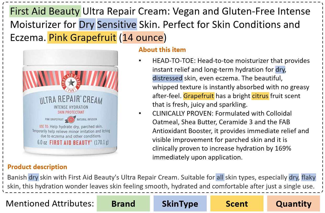
Figure 1: An example of the product profile on an e-Commerce platform. It consists of a title, several information bullets, and a product description.

Most existing studies on attribute value extraction use neural sequence labeling architectures (Zheng et al., 2018; Karamanolakis et al., 2020; Xu et al., 2019). To handle multiple attributes, one line of previous contributions develops a set of “attribute-specific” models (i.e., one model per attribute). The goal is to construct neural networks with (partially) separate model parameters for different attributes. For example, one can construct an independent sequence labeling model for each attribute and make predictions with all the models collectively (e.g., the vanilla OpenTag model (Zheng et al., 2018)). Instead of totally separate models, one can also use different tag sets corresponding to different attributes. These networks can also share the feature encoder and use separate label decoders (Yang et al., 2017). However, the explicit network (component) separation in these contributions constrains knowledge-sharing across different attributes. Exposure to other attributes can help in disambiguating the values for each attribute. And having access to the entire training data for all attributes helps with the generic sequence tagging task. Another line for multi-attribute extraction contributions learns a single model for all attributes. The model proposed by Xu et al. (2019), for example, embeds the attribute name with the textual sequence, to achieve a single “attribute-aware” extraction model for all attributes. This approach addresses the issues in the previous direction. However, sharing all the network parameters with all attributes could limit the model’s capacity to capture attribute-specific characteristics.

In this paper we address the limitations of the existing contribution lines, through adaptive decoder parameterization. We propose to generate a decoder on the fly for each attribute based on its embedding. This results in different but semantically correlated decoders, which maintain the specific characteristics for each attribute, while facilitating knowledge-sharing across different attributes. To this end, we use conditional random fields (CRF) (Lafferty et al., 2001) as the decoders, and parameterize the decoding layers with the attribute embedding through a hypernetwork (Ha et al., 2017) and a Mixture-of-Experts (MoE) module (Jacobs et al., 1991). We further explore several pretrained attribute embedding techniques, to add useful attribute-specific external signals. We use both contextualized and static embeddings for the attribute name along with its potential values to capture meaningful semantic representations.

We summarize our contributions as follows: (1) We propose a multi-attribute value extraction model with an adaptive CRF-based decoder. Our model allows for knowledge sharing across different attributes, yet maintains the individual characteristics of each attribute. (2) We propose several attribute embedding methods, that provide important external semantic signals to the model. (3) We conduct extensive experiments on a real-world e-Commerce dataset, and show improvements over previous methods. We also draw insights on the behavior of the model and the attribute value extraction task itself.

2 Background

2.1 Problem Definition

The main goal of the task is to extract the corresponding values for a given attribute, out of a number of attributes of interest, from the text sequence of a product profile. Formally, given a text sequence $X=[x_{1},\ldots,x_{n}]$ in a product profile, where $n$ is the number of words, and a query attribute $r\in{R}$, where $R$ is a predefined set of attributes, the model is expected to extract all text spans from $X$ that could be valid values for attribute $r$ characterizing this product. When there are no corresponding values mentioned in $X$, the model should return an empty set. For example, for the product in Figure 1, given its title as $X$, the model is expected to return (“Dry”, “Sensitive”) if $r=$“SkinType”, and an empty set if $r=$“Color”.

Following standard approaches (Zheng et al., 2018; Xu et al., 2019; Karamanolakis et al., 2020), under the assumption that different values for an attribute do not overlap in the text sequence, we formulate the value extraction task as a sequence tagging task with the BIOE tagging scheme. That is, given $X$ and $r$, we want to predict a tag sequence $Y=[y_{1},\ldots,y_{n}]$, where $y_{i}\in\{\text{B},\text{I},\text{O},\text{E}\}$ is the tag for $x_{i}$. “B”/“E” indicates the corresponding word is the beginning/ending of an attribute value, “I” means the word is inside an attribute value, and “O” means the word is outside any attribute value. Table 1 shows an example of the tag sequence for attribute “Scent” of a shower gel collection, where “orchid”, “cherry pie”, “mango ice cream” could be extracted as the values.

X	orchid	/	cherry	pie	/	mango	ice	cream	scent
Y	B	O	B	E	O	B	I	E	O

Table 1: An example of the tag sequence for attribute “Scent” annotated with the BIOE scheme.

2.2 BiLSTM-CRF Architecture

The BiLSTM-CRF architecture (Huang et al., 2015) consists of a BiLSTM-based text encoder, and a CRF-based decoder. This architecture has been proven to be effective for the attribute value extraction task (Zheng et al., 2018; Xu et al., 2019; Karamanolakis et al., 2020). We build our AdaTag model based on the BiLSTM-CRF architecture as we find that the BiLSTM-CRF-based models generally perform better than their BiLSTM-based, BERT-based (Devlin et al., 2019) and BERT-CRF-based counterparts, as shown in §5. We introduce the general attribute-agnostic BiLSTM-CRF architecture, which our model is based on, in this subsection.

Given a text sequence $X=[x_{1},\ldots,x_{n}]$. We obtain the sequence of word embeddings $\mathbf{X}=[\mathbf{x}_{1},\ldots,\mathbf{x}_{n}]$ using an embedding matrix $\mathbf{W}_{\text{word}}$. We get the hidden representation of each word by feeding $\mathbf{X}$ into a bi-directional Long-Short Term Memory (LSTM) (Hochreiter and Schmidhuber, 1997) layer with hidden size $d_{h}$:

$$[\mathbf{h}_{1},\ldots,\mathbf{h}_{n}]=\texttt{BiLSTM}([\mathbf{x}_{1},\ldots,\mathbf{x}_{n}]).$$ (1)

We use a CRF-based decoder to decode the sequence of hidden representations while capturing the dependency among tags (e.g., “I” can only be followed by “E”). It consists of a linear layer and a transition matrix, which are used to calculate the emission score and the transition score for the tag prediction respectively. Let $V=[\text{B},\text{I},\text{O},\text{E}]$ be the vocabulary of all possible tags. We calculate an emission score matrix $\mathbf{P}=[\mathbf{p}_{1},\ldots,\mathbf{p}_{n}]\in\mathbb{R}^{4\times n}$, where $\mathbf{P}_{ij}$ is the score for assigning the $i$-th tag in $V$ to $x_{j}$. This is computed by feeding $[\mathbf{h}_{1},\ldots,\mathbf{h}_{n}]$ into a linear layer with parameters $[\mathbf{W},\mathbf{b}]$, specifically $\mathbf{p}_{i}=\mathbf{Wh}_{i}+\mathbf{b}\in\mathbb{R}^{4}$, where $\mathbf{W}\in\mathbb{R}^{4\times d_{h}}$ and $\mathbf{b}\in\mathbb{R}^{4}$. For a BIOE tag sequence $Y=[y_{1},\ldots,y_{n}]$, we get its index sequence $Z=[z_{1},\ldots,z_{n}]$ where $z_{i}\in\{1,2,3,4\}$ is the index of $y_{i}$ in $V$. The score for an input text sequence $X$ to be assigned with a tag sequence $Y$ is calculated as:

$$s(X,Y)=s(X,Z)=\sum_{i=1}^{n-1}\mathbf{T}_{z_{i}z_{i+1}}+\sum_{i=1}^{n}\mathbf{P}_{z_{i}i},$$ (2)

where $\mathbf{T}\in\mathbb{R}^{4\times 4}$ is the transition matrix of CRF, such that $\mathbf{T}_{ij}$ is the score of a transition from the $i$-th tag to the $j$-th tag in $V$.

3 Method

3.1 Model Overview

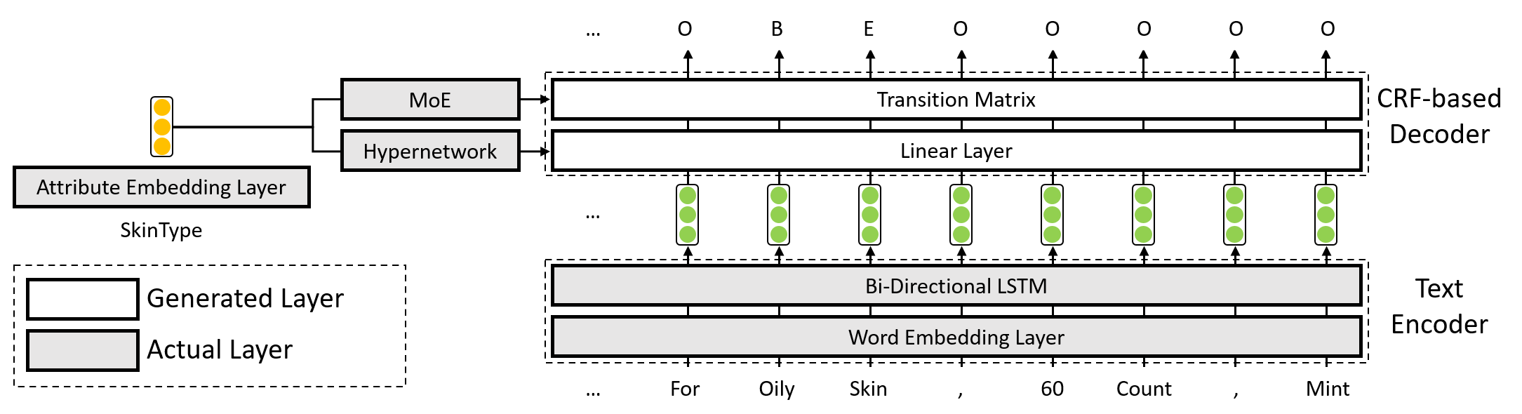
Figure 2: Model architecture. AdaTag equips the BiLSTM-CRF architecture with an adaptive CRF-based decoder.

The multi-attribute value extraction task can be thought of as a group of extraction subtasks, corresponding to different attributes. While all attributes share the general knowledge about value extraction, each has its specificity. The key idea in our proposed model is to dynamically adapt the parameters of the extraction model based on the specific subtask corresponding to the given attribute. We use a BiLSTM-CRF (Huang et al., 2015) architecture, where different subtasks, corresponding to different attributes, share the same text encoder to derive a contextualized hidden representation for each word. Then the hidden representations of the text sequence are decoded into a sequence of tags with a CRF-based decoder, the parameters of which are generated on the fly based on the attribute embedding. In this setup, different subtasks are trained jointly, and different decoders are correlated based on the attribute embedding. This facilitates a knowledge-sharing scheme across different attributes. Intuitively, this can help with learning generic abilities like detecting value boundary, which is at the core of the extraction process of any attribute. At the same time, our model provides each subtask with a customized decoder parameterization, which improves the model’s capacity for capturing attribute-specific knowledge.

Figure 2 presents our overall model architecture, where we equip the BiLSTM-CRF architecture with an adaptive CRF-based decoder. In §3.2, we will introduce our adaptive CRF-based decoder which is parameterized with the attribute embedding. In §3.3, we will describe how to obtain pretrained attribute embeddings that can capture the characteristics of different subtasks, so that “similar” attributes get “similar” decoding layers.

3.2 Adaptive CRF-based Decoder

In attribute value extraction, the model takes the text sequence $X$ with a query attribute $r$ as input, and is expected to predict $Y$ based on both $X$ and $r$. To make the model aware of the query attribute, we need to incorporate the attribute information into some components of the BiLSTM-CRF architecture. The BiLSTM-based text encoder is responsible for encoding the text sequence and obtain a contextualized representation for each word, which can be regarded as “understanding” the sentence. The CRF-based decoder then predicts a tag for each word based on its representation. Therefore, we propose that all attributes share a unified text encoder so that the representation can be enhanced through learning with different subtasks, and each attribute has a decoder adapted to its corresponding subtask, the parameters of which are generated based on the attribute information.

As introduced in §2.2, a CRF-based decoder consists of a linear layer and a transition matrix. The linear layer takes hidden representations as input, and predicts a tag distribution for each word independently. It captures most of characteristics of value extraction for a given attribute based on the text understanding. More flexibility is needed to model the specificity of different attributes. By contrast, the transition matrix learns the dependency among tags to avoid predicting unlikely tag sequence. It only captures shallow characteristics for the attribute based on its value statistics. For example, the transition scores form “B” to other tags largely depend on the frequent lengths of the attribute values. If single-word values are mentioned more often, then “B” is more likely to be followed by “O”. If two-word values dominate the vocabulary, then “B” is more likely to be followed by “E”. Attributes could be simply clustered based on these shallow characteristics.

In this work we parameterize the CRF-based decoder with the attribute embedding $\mathbf{r}\in\mathbb{R}^{d_{r}}$, where $d_{r}$ is the dimension of the attribute embedding. For the linear layer, we adopt a hypernetwork (Ha et al., 2017) due to its high flexibility. For the transition matrix, we develop a Mixture-of-Experts (Pahuja et al., 2019) module to leverage the latent clustering nature of attributes. We nevertheless experiment with all 4 combinations of these methods in §5.3, and this choice does the best.

Hypernetwork.

The idea of hypernetworks (Ha et al., 2017) is to use one network to generate the parameters of another network. Such approach has high flexibility when no constraint is imposed during generation. We therefore use it to parameterize the linear layer. In our model, we learn two different linear transformations that map the attribute embedding to the parameters of the linear layer ($\mathbf{W}\in\mathbb{R}^{4\times d_{h}}$, $\mathbf{b}\in\mathbb{R}^{4}$) in the CRF-based decoder:

$$\begin{split}\mathbf{W}&=\texttt{Reshape}(\mathbf{W}_{\text{hyper}}^{w}\mathbf{r}+\mathbf{b}_{\text{hyper}}^{w}),\\ \mathbf{b}&=\texttt{Reshape}(\mathbf{W}_{\text{hyper}}^{b}\mathbf{r}+\mathbf{b}_{\text{hyper}}^{b}).\end{split}$$ (3)

Here $\mathbf{W}_{\text{hyper}}^{w}\in\mathbb{R}^{4d_{h}\times d_{r}}$, $\mathbf{b}_{\text{hyper}}^{w}\in\mathbb{R}^{4d_{h}}$, $\mathbf{W}_{\text{hyper}}^{b}\in\mathbb{R}^{4\times d_{r}}$, $\mathbf{b}_{\text{hyper}}^{b}\in\mathbb{R}^{4}$, and the Reshape operator reshapes a $1$-D vector into a matrix with the same number of elements.

Mixture-of-Experts.

The idea of Mixture-of-Experts (Jacobs et al., 1991) is to have a group of networks (“experts”) that jointly make decisions with dynamically determined weights. Unlike previous approaches that combine each expert’s prediction, we combine their parameters for generating the transition matrix. Let $k$ be the number of experts we use to parameterize the transition matrix $\mathbf{T}\in\mathbb{R}^{4\times 4}$ where $k$ is a hyperparameter. We introduce $k$ learnable matrices $\mathbf{T}^{(1)},\ldots,\mathbf{T}^{(k)}$ for the $k$ experts. Each expert’s matrix can be understood as a cluster prototype and we employ a linear gating network to compute the probability of assigning the given attribute to each expert: $\bm{\lambda}=\texttt{Softmax}(\mathbf{W}_{\text{moe}}\mathbf{r}+\mathbf{b}_{\text{moe}})$. Here $\mathbf{W}_{\text{moe}}\in\mathbb{R}^{k\times d_{r}}$, $\mathbf{b}_{\text{moe}}\in\mathbb{R}^{k}$, $\bm{\lambda}=[\lambda_{1},\ldots,\lambda_{k}]\in\mathbb{R}^{k}$ and $\sum_{i=1}^{k}\lambda_{i}=1$. The parameters for the transition matrix for this attribute is calculated as: $\mathbf{T}=\sum_{i=1}^{k}\lambda_{i}\mathbf{T}^{(i)}$.

3.3 Pretrained Attribute Embeddings

The attribute embedding $\mathbf{r}$ plays a key role in deriving the attribute-specific decoding layers. Therefore, the quality of the attribute embeddings is crucial to the success of our parameterization method. Good attribute embeddings are supposed to capture the subtask similarities such that similar extraction tasks use decoders with similar parameters. In this work, we propose to use the attribute name and possible values as a proxy to capture the characteristics of the value extraction task for a given attribute. The attribute embeddings can therefore be directly derived from the training data and loaded into the attribute embedding layer as initialization.

For each attribute $r$, we first collect all the sentences from the training data that are annotated with at least one value for $r$. We denote the collected sentences with values as $D_{r}=\{(\tilde{r},v_{i},X_{i})\}_{i=1}^{n_{r}}$ where $\tilde{r}$ is the phrase representation of $r$ (e.g., $\tilde{r}=$ “Skin Type” if $r=$ “SkinType”), $v_{i}$ is a span in text sequence $X_{i}$ that serves as the value for $r$, and $n_{r}$ is the number of collected sentences. For each $(\tilde{r},v_{i},X_{i})$, we can calculate an attribute name embedding $\mathbf{r}_{i}^{\text{name}}$ and an attribute value embedding $\mathbf{r}_{i}^{\text{value}}$ in either a contextualized way or an uncontextualized way, which are detailed later. We pool over all instances in $D_{r}$ to get the final attribute name embedding and attribute value embedding, which are concatenated as the attribute embedding: $\mathbf{r}^{\text{name}}=\frac{1}{n_{r}}\sum_{i=1}^{n_{r}}\mathbf{r}_{i}^{\text{name}}$, $\mathbf{r}^{\text{value}}=\frac{1}{n_{r}}\sum_{i=1}^{n_{r}}\mathbf{r}_{i}^{\text{value}}$, $\mathbf{r}=\texttt{Concat}(\mathbf{r}^{\text{name}},\mathbf{r}^{\text{value}})$.

Contextualized Embeddings.

Taking the context into consideration helps get embeddings that can more accurately represent the semantics of the word. Here we use the contextualized representations provided by BERT (Devlin et al., 2019) to generate the embedding. We use BERT to encode $X_{i}$ and get $v_{i}$’s phrase embedding (the averaged embedding of each word in the phrase) as $\mathbf{r}_{i}^{\text{value}}$. By replacing $v_{i}$ with “[BOA] $\tilde{r}$ [EOA]” and encoding the modified sequence with BERT, we get the phrase embedding for “[BOA] $\tilde{r}$ [EOA]” as $\mathbf{r}_{i}^{\text{name}}$.

Uncontextualized Embeddings.

Static embeddings like Word2Vec (Mikolov et al., 2013) and Glove (Pennington et al., 2014) can be more stable to use under noisy contexts. We use Glove (50d) to get the phrase embedding for $v_{i}$ as $\mathbf{r}_{i}^{\text{value}}$ and the phrase embedding for $\tilde{r}$ as $\mathbf{r}_{i}^{\text{name}}$.

3.4 Model Training

As we parameterize the CRF-based decoder with the attribute embedding through MoE and hypernetwork, the learnable parameters in our model includes $\boldsymbol{\uptheta}_{\text{encoder}}=\{\mathbf{W}_{\text{word}},\boldsymbol{\uptheta}_{\text{bi-lstm}}\}$, $\boldsymbol{\uptheta}_{\text{hyper}}=\{\mathbf{W}_{\text{hyper}}^{w},\mathbf{b}_{\text{hyper}}^{w},\mathbf{W}_{\text{hyper}}^{b},\mathbf{b}_{\text{hyper}}^{b}\}$, $\boldsymbol{\uptheta}_{\text{moe}}=\{\mathbf{W}_{\text{moe}},\mathbf{b}_{\text{moe}},\{\mathbf{T}^{(i)}\}_{i=1}^{k}\}$. We freeze the attribute embeddings $\mathbf{W}_{\text{att}}$ as it gives better performance, which is also discussed in §5.3.

The whole model is trained end-to-end by maximizing the log likelihood of $(X,r,Y)$ triplets in the training set, which is derived from Equation 2 as:

$$\begin{split}s(X,r,Y)&=\sum_{i=0}^{n}\mathbf{T}_{z_{i}z_{i+1}}+\sum_{i=1}^{n}\mathbf{P}_{z_{i}i},\\ \log p(Y\mid X,r)&=\log\frac{s(X,r,Y)}{\sum_{Y^{\prime}\in V^{n}}s(X,r,Y^{\prime})},\end{split}$$ (4)

where $V_{n}$ is the set of all tag sequences of length $n$. The log likelihood can be computed efficiently using the forward algorithm (Baum and Eagon, 1967) for hidden Markov models (HMMs). At inference, we adopt Viterbi algorithm (Viterbi, 1967) to get the most likely $Y$ given $X$ and $r$ in test set.

4 Experimental Setup

4.1 Dataset

To evaluate the effectiveness of our proposed model, we build a dataset by collecting product profiles (title, bullets, and description) from the public web pages at Amazon.com.

Following previous works (Zheng et al., 2018; Karamanolakis et al., 2020; Xu et al., 2019), we obtain the attribute-value pairs for each product using the product information on the webpages by distant supervision. We select 32 attributes with different frequencies. For each attribute, we collect product profiles that are labeled with at least one value for this attribute. We further split the collected data into training (90%) and development (10%) sets.

The annotations obtained by distant supervision are often noisy so they cannot be considered as gold labels. To ensure the reliability of the evaluation results, we also manually annotated an additional testing set covering several attributes. We randomly selected 12 attributes from the 32 training attributes, took a random sample from the relevant product profiles for each attribute, and asked human annotators to annotate the corresponding values. We ensured that there is no product overlapping between training/development sets and the test set.

Putting together the datasets built for each individual attribute, we end up with training and development sets for 32 attributes, covering 333,857 and 40,008 products respectively. The test set has 12 attributes and covers 11,818 products. Table 2 presents the statistics of our collected dataset. Table 3 shows the attribute distribution of the training set. It clearly demonstrates the data imbalance issue of the real-world attribute value extraction data.

Most of the attribute values are usually covered in the title and bullets, since sellers would aim to highlight the product features early on in the product profile. The description, on the other hand, can provide few new values complementing those mentioned in the title and bullets, but significantly increases the computational costs due to its length. Therefore, we consider two settings for experiments: extracting from the title only (“Title”) and extracting from the concatenation of the title and bullets (“Title + Bullets”).

Split	# Attributes	# Products	Avg. # Words (Title)	Avg. # Words (Title+Bullets)
train	32	333,857	20.9	113.4
dev	32	40,008	21.0	113.7
test	12	11,818	20.5	120.0

Table 2: Statistics of our collected dataset.

# Products	# Att.	Examples
$[10000,50279]$	$12$	Color, Flavor, SkinType, HairType
$[1000,10000)$	$10$	ActiveIngredients, CaffeineContent
$[100,1000)$	$6$	SpecialIngredients, DosageForm
$[15,100)$	$4$	PatternType, ItemShape

Table 3: Frequencies of different attributes in the training set.

4.2 Evaluation Metrics

For each attribute, we calculate Precision/Recall/F₁ based on exact string matching. That is, an extracted value is considered correct only if it exactly matches one of the ground truth values for the query attribute in the given text sequence. We use Macro-Precision/Macro-Recall/Macro-F₁ (denoted as P/R/F₁) as the aggregated metrics to avoid bias towards high-resource attributes. They are calculated by averaging per-attribute metrics.

4.3 Compared Methods

We compare our proposed model with a series of strong baselines for attribute value extraction.

BiLSTM uses a BiLSTM-based encoder. Each hidden representation is decoded independently into a tag with a linear layer followed by softmax. BiLSTM-CRF (Huang et al., 2015) uses a BiLSTM-based encoder and a CRF-based decoder, as described in §2.2. Zheng et al. (2018) propose OpenTag, which uses a self-attention layer between the BiLSTM-based encoder and CRF-based decoder for interpretable attribute value extraction. However, we find the self-attention layer not helpful for the performance. We therefore only present the results for BiLSTM-CRF in §5. BERT (Devlin et al., 2019) and BERT-CRF replace the BiLSTM-based text encoder with BERT.

Note that these four methods don’t take the query attribute as input. To make them work in our more realistic setting with multiple ($N$) attributes, we consider two variants for each of them. (1) “$N$ tag sets”: We introduce one set of B/I/E tags for each attribute, so that a tag sequence can be unambiguously mapped to the extraction results for multiple attributes. For example, the tag sequence “B-SkinType E-SkinType O B-Scent” indicates that the first two words constitutes a value for attribute SkinType, and the last word is a value for Scent. Only one model is needed to handle the extraction for all attributes. (2) “$N$ models”: We build one value extraction model for each attribute — we’ll train $N$ models for this task.

The “$N$ models” variant isolates the learning of different attributes. To enable knowledge sharing, other methods share the model components or the whole model among all attributes: BiLSTM-CRF-SharedEmb shares a word embedding layer among all attributes. Each attribute has its own BiLSTM layer and CRF-based decoder, which are independent from each other. BiLSTM-MultiCRF (Yang et al., 2017) shares a BiLSTM-based text encoder among all attributes. Each attribute has its own CRF-based decoder. SUOpenTag (Xu et al., 2019) encodes both the text sequence and the query attribute with BERT and adopts a cross-attention mechanism to get an attribute-aware representation for each word. The hidden representations are decoded into a tags with a CRF-based decoder.

We also include AdaTag (Random AttEmb), which has the same architecture as our model but uses randomly initialized learnable attribute embeddings of the same dimension.

4.4 Implementation Details

We implement all models with PyTorch (Paszke et al., 2019). For models involving BERT, we use the bert-base-cased version. Other models use pretrained 50d Glove (Pennington et al., 2014) embeddings as the initialization of the word embedding matrix $\mathbf{W}_{\text{word}}$. We choose $d_{h}=200$ as the hidden size of the BiLSTM layer and 32 as the batch size. BERT-based models are optimized using AdamW (Loshchilov and Hutter, 2019) optimizer with learning rate $2e^{-5}$. Others use the Adam (Kingma and Ba, 2015) optimizer with learning rate $1e^{-3}$. We perform early stopping if no improvement in (Macro-) F₁ is observed on the development set for 3 epochs. For our model, we use contextualized attribute embeddings as described in §3.2 and freeze them during training. We set $k=3$ for MoE. We made choices based on the development set performance.

5 Experimental Results

5.1 Overall Results

Table 4 presents the overall results using our dataset under both “Title” and “Title + Bullets” settings. Our model demonstrates great improvements over baselines on all metrics except getting second best recall under the “Title + Bullets” settings. The comparisons demonstrate the overall effectiveness of our model and pretrained attribute embeddings.

Methods	Title			Title + Bullets
	P(%)	R(%)	F1(%)	P(%)	R(%)	F1(%)
Group I: $N$ tag sets
BiLSTM ($N$ tag sets)	35.15	54.28	38.92	32.17	34.30	31.18
BiLSTM-CRF ($N$ tag sets)	35.23	53.94	38.85	34.03	35.01	32.11
BERT ($N$ tag sets)	33.52	50.48	36.29	31.41	30.62	28.26
BERT-CRF ($N$ tag sets)	34.55	51.96	37.45	32.63	31.24	28.89
Group II: $N$ models
BiLSTM ($N$ models)	64.37	71.71	64.64	61.61	60.26	58.56
BiLSTM-CRF ($N$ models)	63.94	72.14	64.78	62.07	61.46	59.19
BERT ($N$ models)	55.34	72.86	58.48	53.35	61.27	54.37
BERT-CRF ($N$ models)	54.29	72.79	57.49	49.25	59.33	50.49
Group III: shared components
BiLSTM-CRF-SharedEmb	63.77	72.50	64.62	58.95	60.58	57.66
BiLSTM-MultiCRF	64.48	72.04	64.81	60.64	62.75	59.78
SUOpenTag	63.62	71.67	64.76	61.57	60.48	59.62
AdaTag (Random AttEmb)	64.80	71.95	65.74	60.14	62.14	60.04
AdaTag (Our Model)	65.00	75.87	67.48	62.87	62.45	60.87

Table 4: Performance comparison on test set with 12 attributes (best in boldface and second best underlined).

The “$N$ tag sets” variants get much lower performance than other methods, probably due to the severe data imbalance issue in the training set (see Table 3). All attributes share the same CRF-based decoder, which could make learning biased towards high-resource attributes. Note that introducing one set of tags for each entity type is the standard approach for the Named Entity Recognition (NER) task. Its low performance suggests that the attribute value extraction task is inherently different from standard NER.

Variants of “shared components” generally achieve higher performance than the independent modeling methods (“$N$ models”), which demonstrates the usefulness of enabling knowledge sharing among different subtasks.

We also notice that BERT and BERT-CRF models get lower performance than their BiLSTM and BiLSTM-CRF counterparts. The reason could be the domain discrepancy between the corpora that BERT is pretrained on and the product title/bullets. The former consist of mainly natural language sentences, while the latter are made up of integration of keywords and ungrammatical sentences.

5.2 High- vs. Low-Resource Attributes

To better understand the gain achieved by joint modeling, we further split the 12 testing attributes into 8 high-resource attributes and 4 low-resource attributes, based on the size of the training data with $1000$ instances as the threshold. It is important to point out that many factors (e.g., vocabulary size, value ambiguity, and domain diversity), other than the size of training data, can contribute to the difficulty of modeling an attribute. Therefore, the performance for different attributes is not directly comparable.

From results in Table 5, we can see that our model gets a lot more significant improvement from the independent modeling approach (BiLSTM-CRF ($N$ models)) on low-resource attributes compared to high-resource attributes. This suggests that low-resource attributes benefit more from knowledge sharing, making our model desirable in the real-world setting with imbalanced attribute distribution.

Methods	High-Resource Att.			Low-Resource Att.
	P(%)	R(%)	F1(%)	P(%)	R(%)	F1(%)
BiLSTM-CRF ($N$ models)	54.04	75.66	61.57	83.72	65.08	71.19
BiLSTM-MultiCRF	54.38	74.42	60.23	84.70	67.29	73.97
SUOpenTag	55.34	72.94	60.49	80.16	69.13	73.31
AdaTag (Our Model)	56.05	76.07	62.00	82.90	75.48	78.45

Table 5: Performance comparison on high-resource and low-resource attributes.

5.3 Ablation Studies

Attribute Embeddings.

We study different choices of adopting pretrained attribute embeddings. Specially, we experiment with contextualized embeddings (BERT${}_{\text{name+value}}$) and uncontextualized embeddings (Glove${}_{\text{name+value}}$) under the “Title” setting. For given attribute embeddings, we can either finetune them during training or freeze them once loaded. We also experiment with attribute name embeddings $\mathbf{r}^{\text{name}}$ and attribute value embeddings $\mathbf{r}^{\text{value}}$ only to understand which information is more helpful. The baseline is set as using randomly initialized learnable attribute embeddings. Table 6 shows the results. Comparing attribute embeddings with the same dimension, we find that freezing pretrained embeddings always leads to performance gain over the random baseline. This is because our parameterization methods have high flexibility in generating the parameters for the decoder. Using pretrained embeddings and freezing them provides the model with a good starting point and makes learning easier by reducing the degree of freedom. BERT${}_{\text{name}}$ (freeze) outperforms BERT${}_{\text{value}}$ (freeze), suggesting that the attribute name is more informative in determining the characteristics of the value extraction task on our dataset, where the values labeled through distant supervision are noisy.

Attribute Embeddings	Dimension	P(%)	R(%)	F1(%)
Random	100	63.05	72.35	64.82
Glove${}_{\text{name+value}}$	100	64.12	70.51	63.89
Glove${}_{\text{name+value}}$ (freeze)	100	64.47	73.11	65.53
Random	768	63.83	72.39	65.12
BERT${}_{\text{name}}$	768	62.01	73.94	64.89
BERT${}_{\text{name}}$ (freeze)	768	64.90	74.31	66.60
BERT${}_{\text{value}}$	768	65.03	72.36	65.53
BERT${}_{\text{value}}$ (freeze)	768	62.96	73.92	65.51
Random	1536	64.80	71.95	65.74
BERT${}_{\text{name+value}}$	1536	63.57	73.57	65.81
BERT${}_{\text{name+value}}$ (freeze)	1536	65.00	75.87	67.48

Table 6: Performance (Title) with different choices for deriving and adopting attribute embeddings.

Linear Layer	Transition Matrix	P(%)	R(%)	F1(%)
MoE	MoE	42.28	65.80	47.94
hypernetwork	hypernetwork	65.59	69.39	63.66
MoE	hypernetwork	53.52	66.43	55.10
hypernetwork	MoE	65.00	75.87	67.48

Table 7: Performance (Title) with different parameterization methods.

Decoder Parameterization.

We study different design choices for parameterizing the CRF-based decoder. For designs involving MoE, we search the number of experts ($k$) in $[1,2,3,4,5]$ and adopt the best one to present the results. We experiment under the “Title” setting. From Table 7, we find that parameterizing the linear layer with MoE leads to much lower performance. This is reasonable because the linear layer plays a much more important role in the decoder while the transition matrix acts more like a regularization to avoid bad tag sequences. MoE uses $k$ matrices as basis and expects to represent the parameters for any attribute as a linear combination of the bases. That limits the expressiveness to capture complicated characteristics of different attributes and will thus severely hurt the performance. As for the transition matrix, modeling with MoE is a better choice. This is because the transition matrix is more “structured” in the sense that each of it element is expected to be either a big number or a small number based on its semantics. For example, the transition score for $\text{I}\rightarrow\text{E}$ should be much higher than $\text{I}\rightarrow\text{B}$. Hypernetwork is too flexible to generate such “structured” parameters.

5.4 Effect of Number of Attributes

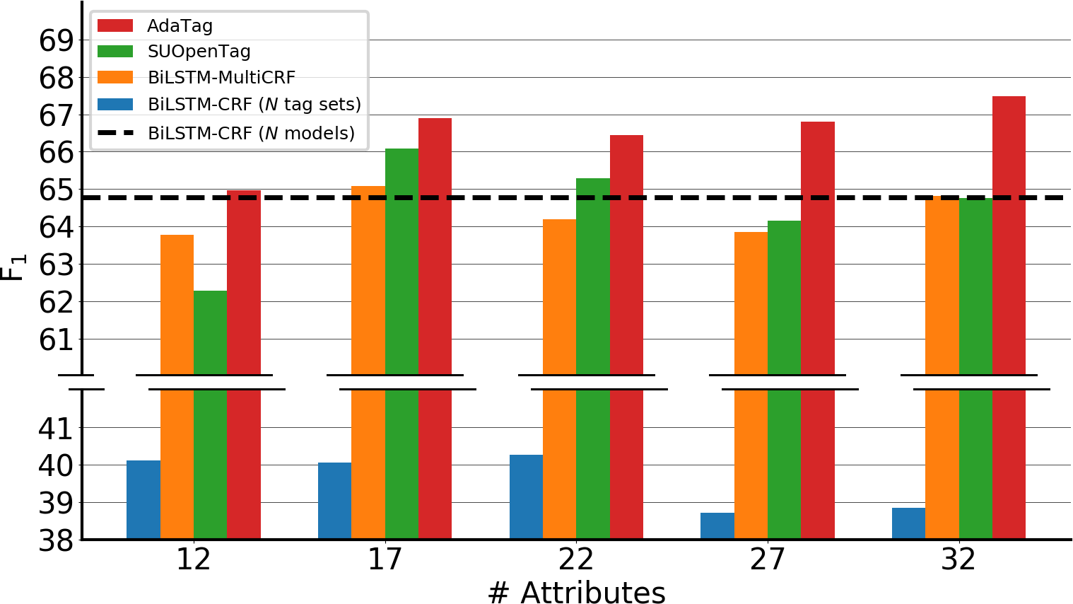
Figure 3: Performance (Title) with different numbers of training attributes. We use broken y-axis due to the large gap in results between BiLSTM-CRF ($N$ tag sets) and other models.

An important motivation of our model is that joint modeling of different attributes can facilitate knowledge sharing and improve the performance. Here we study the performance of model improvement along with increment of the number of jointly modeled attributes. We experiment under the “Title” setting. We start with training our model on 12 attributes that have test data. After that, we random select 5, 10, 15, 20 attributes from the remaining attributes, and add them to the joint training. The evaluation results on 12 test attributes are presented in Figure 3. While our model general demonstrates greater improvement with joint modeling of more attributes, other models’ performance fluctuate or goes down. That also demonstrates the scalability of our model when new attributes keep emerging in real-world scenarios.

6 Related Work

Attribute Value Extraction.

OpenTag (Zheng et al., 2018) formulates attribute value extraction as a sequence tagging task, and proposes a BiLSTM-SelfAttention-CRF architecture to address the problem. Xu et al. (2019) propose an “attribute-aware” setup, by utilizing one set of BIO tags and attribute name embedding with an attention mechanism, to enforce the extraction network to be attribute comprehensive. Karamanolakis et al. (2020) additionally incorporate the product taxonomy into a multi-task learning setup, to capture the nuances across different product types. Zhu et al. (2020) introduce a multi-modal network to combine text and visual information with a cross-modality attention to leverage image rich information that is not conveyed in text. Wang et al. (2020) use a question answering formulation to tackle attribute value extraction. We adopt the extraction setup in our model as most of previous contributions, using sequence labeling architecture. But we utilize an adaptive decoding approach, where the decoding network is parameterized with the attribute embedding.

Dynamic Parameter Generation.

Our model proposes an adaptive-based decoding setup, parameterized with attribute embeddings through a Mixture-of-Experts module and a hypernetwork. Jacobs et al. (1991) first propose a system composed of several different “expert” networks and use a gating network that decides how to assign different training instances to different “experts”. Alshaikh et al. (2020); Guo et al. (2018); Le et al. (2016); Peng et al. (2019) all use domain/knowledge experts, and combine the predictions of each expert with a gating network. Unlike these works, we combine the weights of each expert to parameterize a network layer given an input embedding. Ha et al. (2017) propose the general idea of generating the parameters of a network by another network. The proposed model in Cai et al. (2019) generates the parameters of an encoder-decoder architecture by referring to the context-aware and topic-aware input. Suarez (2017) uses a hypernetwork to scale the weights of the main recurrent network. Platanios et al. (2018) tackle neural machine translation between multiple languages using a universal model with a contextual parameter generator.

7 Conclusion

In this work we propose a multi-attribute value extraction model that performs joint modeling of many attributes using an adaptive CRF-based decoder. Our model has a high capacity to derive attribute-specific network parameters while facilitating knowledge sharing. Incorporated with pretrained attribute embeddings, our model shows marked improvements over previous methods.

Appendix A Number of Model Parameters

Methods	# Parameters
BiLSTM ($\mathbf{N}$ tag sets)	$0.6k\cdot\mathbf{N}+6M$
BiLSTM-CRF ($\mathbf{N}$ tag sets)	$9\cdot\mathbf{N}^{2}+0.6k\cdot\mathbf{N}+6M$
BiLSTM/BiLSTM-CRF ($\mathbf{N}$ models)	$6M\cdot\mathbf{N}$
BiLSTM-CRF-SharedEmb	$0.1M\cdot\mathbf{N}+6M$
BiLSTM-MultiCRF	$2k\cdot\mathbf{N}+6M$
AdaTag	$8M$

Table 8: Numbers of parameters for BiLSTM-based models with $\mathbf{N}$ attributes.

In our main experiment (Table 4), the numbers of parameters ($M=1,000,000$; $k=1,000$) for BiLSTM-based models with $\mathbf{N}$ attributes are listed in Table 8. BERT (bert-base-cased) itself has $110M$ parameters, making BERT-based models generally much larger.

For our AdaTag, the weights for the hypernetwork ($\mathbf{W}_{\text{hyper}}^{w}\in\mathbb{R}^{4d_{h}\times d_{r}}$) have $(4\times 200)\times 1536$ parameters. The number can be reduced by inserting a middle layer with fewer neurons.

References

- Ai et al. (2017) Qingyao Ai, Yongfeng Zhang, Keping Bi, Xu Chen, and W. Bruce Croft. 2017. Learning a hierarchical embedding model for personalized product search. In Proceedings of the 40th International ACM SIGIR Conference on Research and Development in Information Retrieval, Shinjuku, Tokyo, Japan, August 7-11, 2017, pages 645–654. ACM.
- Alshaikh et al. (2020) Rana Alshaikh, Zied Bouraoui, Shelan Jeawak, and Steven Schockaert. 2020. A mixture-of-experts model for learning multi-facet entity embeddings. In Proceedings of the 28th International Conference on Computational Linguistics, pages 5124–5135, Barcelona, Spain (Online). International Committee on Computational Linguistics.
- Baum and Eagon (1967) Leonard E Baum and John Alonzo Eagon. 1967. An inequality with applications to statistical estimation for probabilistic functions of markov processes and to a model for ecology. Bulletin of the American Mathematical Society, 73(3):360–363.
- Cai et al. (2019) Hengyi Cai, Hongshen Chen, Cheng Zhang, Yonghao Song, Xiaofang Zhao, and Dawei Yin. 2019. Adaptive parameterization for neural dialogue generation. In Proceedings of the 2019 Conference on Empirical Methods in Natural Language Processing and the 9th International Joint Conference on Natural Language Processing (EMNLP-IJCNLP), pages 1793–1802, Hong Kong, China. Association for Computational Linguistics.
- Devlin et al. (2019) Jacob Devlin, Ming-Wei Chang, Kenton Lee, and Kristina Toutanova. 2019. BERT: Pre-training of deep bidirectional transformers for language understanding. In Proceedings of the 2019 Conference of the North American Chapter of the Association for Computational Linguistics: Human Language Technologies, Volume 1 (Long and Short Papers), pages 4171–4186, Minneapolis, Minnesota. Association for Computational Linguistics.
- Guo et al. (2018) Jiang Guo, Darsh Shah, and Regina Barzilay. 2018. Multi-source domain adaptation with mixture of experts. In Proceedings of the 2018 Conference on Empirical Methods in Natural Language Processing, pages 4694–4703, Brussels, Belgium. Association for Computational Linguistics.
- Ha et al. (2017) David Ha, Andrew M. Dai, and Quoc V. Le. 2017. Hypernetworks. In 5th International Conference on Learning Representations, ICLR 2017, Toulon, France, April 24-26, 2017, Conference Track Proceedings. OpenReview.net.
- Hochreiter and Schmidhuber (1997) Sepp Hochreiter and Jürgen Schmidhuber. 1997. Long short-term memory. Neural computation, 9(8):1735–1780.
- Huang et al. (2015) Zhiheng Huang, Wei Xu, and Kai Yu. 2015. Bidirectional LSTM-CRF models for sequence tagging. CoRR, abs/1508.01991.
- Jacobs et al. (1991) Robert A Jacobs, Michael I Jordan, Steven J Nowlan, and Geoffrey E Hinton. 1991. Adaptive mixtures of local experts. Neural computation, 3(1):79–87.
- Karamanolakis et al. (2020) Giannis Karamanolakis, Jun Ma, and Xin Luna Dong. 2020. TXtract: Taxonomy-aware knowledge extraction for thousands of product categories. In Proceedings of the 58th Annual Meeting of the Association for Computational Linguistics, pages 8489–8502, Online. Association for Computational Linguistics.
- Kingma and Ba (2015) Diederik P. Kingma and Jimmy Ba. 2015. Adam: A method for stochastic optimization. In 3rd International Conference on Learning Representations, ICLR 2015, San Diego, CA, USA, May 7-9, 2015, Conference Track Proceedings.
- Kula (2015) Maciej Kula. 2015. Metadata embeddings for user and item cold-start recommendations. arXiv preprint arXiv:1507.08439.
- Kulkarni et al. (2019) Ashish Kulkarni, Kartik Mehta, Shweta Garg, Vidit Bansal, Nikhil Rasiwasia, and Srinivasan Sengamedu. 2019. Productqna: Answering user questions on e-commerce product pages. In Companion Proceedings of The 2019 World Wide Web Conference, pages 354–360.
- Lafferty et al. (2001) John D. Lafferty, Andrew McCallum, and Fernando C. N. Pereira. 2001. Conditional random fields: Probabilistic models for segmenting and labeling sequence data. In Proceedings of the Eighteenth International Conference on Machine Learning (ICML 2001), Williams College, Williamstown, MA, USA, June 28 - July 1, 2001, pages 282–289. Morgan Kaufmann.
- Le et al. (2016) Phong Le, Marc Dymetman, and Jean-Michel Renders. 2016. LSTM-based mixture-of-experts for knowledge-aware dialogues. In Proceedings of the 1st Workshop on Representation Learning for NLP, pages 94–99, Berlin, Germany. Association for Computational Linguistics.
- Loshchilov and Hutter (2019) Ilya Loshchilov and Frank Hutter. 2019. Decoupled weight decay regularization. In 7th International Conference on Learning Representations, ICLR 2019, New Orleans, LA, USA, May 6-9, 2019. OpenReview.net.
- Mikolov et al. (2013) Tomas Mikolov, Kai Chen, Greg Corrado, and Jeffrey Dean. 2013. Efficient estimation of word representations in vector space. arXiv preprint arXiv:1301.3781.
- Pahuja et al. (2019) Vardaan Pahuja, Jie Fu, and Christopher J. Pal. 2019. Learning sparse mixture of experts for visual question answering. CoRR, abs/1909.09192.
- Paszke et al. (2019) Adam Paszke, Sam Gross, Francisco Massa, Adam Lerer, James Bradbury, Gregory Chanan, Trevor Killeen, Zeming Lin, Natalia Gimelshein, Luca Antiga, Alban Desmaison, Andreas Köpf, Edward Yang, Zachary DeVito, Martin Raison, Alykhan Tejani, Sasank Chilamkurthy, Benoit Steiner, Lu Fang, Junjie Bai, and Soumith Chintala. 2019. Pytorch: An imperative style, high-performance deep learning library. In Advances in Neural Information Processing Systems 32: Annual Conference on Neural Information Processing Systems 2019, NeurIPS 2019, December 8-14, 2019, Vancouver, BC, Canada, pages 8024–8035.
- Peng et al. (2019) Hao Peng, Ankur Parikh, Manaal Faruqui, Bhuwan Dhingra, and Dipanjan Das. 2019. Text generation with exemplar-based adaptive decoding. In Proceedings of the 2019 Conference of the North American Chapter of the Association for Computational Linguistics: Human Language Technologies, Volume 1 (Long and Short Papers), pages 2555–2565, Minneapolis, Minnesota. Association for Computational Linguistics.
- Pennington et al. (2014) Jeffrey Pennington, Richard Socher, and Christopher Manning. 2014. GloVe: Global vectors for word representation. In Proceedings of the 2014 Conference on Empirical Methods in Natural Language Processing (EMNLP), pages 1532–1543, Doha, Qatar. Association for Computational Linguistics.
- Platanios et al. (2018) Emmanouil Antonios Platanios, Mrinmaya Sachan, Graham Neubig, and Tom Mitchell. 2018. Contextual parameter generation for universal neural machine translation. In Proceedings of the 2018 Conference on Empirical Methods in Natural Language Processing, pages 425–435, Brussels, Belgium. Association for Computational Linguistics.
- Suarez (2017) Joseph Suarez. 2017. Language modeling with recurrent highway hypernetworks. In Advances in Neural Information Processing Systems 30: Annual Conference on Neural Information Processing Systems 2017, December 4-9, 2017, Long Beach, CA, USA, pages 3267–3276.
- Viterbi (1967) Andrew Viterbi. 1967. Error bounds for convolutional codes and an asymptotically optimum decoding algorithm. IEEE transactions on Information Theory, 13(2):260–269.
- Wang et al. (2020) Qifan Wang, Li Yang, Bhargav Kanagal, Sumit Sanghai, D. Sivakumar, Bin Shu, Zac Yu, and Jon Elsas. 2020. Learning to extract attribute value from product via question answering: A multi-task approach. In KDD ’20: The 26th ACM SIGKDD Conference on Knowledge Discovery and Data Mining, Virtual Event, CA, USA, August 23-27, 2020, pages 47–55. ACM.
- Xu et al. (2019) Huimin Xu, Wenting Wang, Xin Mao, Xinyu Jiang, and Man Lan. 2019. Scaling up open tagging from tens to thousands: Comprehension empowered attribute value extraction from product title. In Proceedings of the 57th Annual Meeting of the Association for Computational Linguistics, pages 5214–5223, Florence, Italy. Association for Computational Linguistics.
- Yang et al. (2017) Zhilin Yang, Ruslan Salakhutdinov, and William W. Cohen. 2017. Transfer learning for sequence tagging with hierarchical recurrent networks. In 5th International Conference on Learning Representations, ICLR 2017, Toulon, France, April 24-26, 2017, Conference Track Proceedings. OpenReview.net.
- Zheng et al. (2018) Guineng Zheng, Subhabrata Mukherjee, Xin Luna Dong, and Feifei Li. 2018. Opentag: Open attribute value extraction from product profiles. In Proceedings of the 24th ACM SIGKDD International Conference on Knowledge Discovery & Data Mining, KDD 2018, London, UK, August 19-23, 2018, pages 1049–1058. ACM.
- Zhu et al. (2020) Tiangang Zhu, Yue Wang, Haoran Li, Youzheng Wu, Xiaodong He, and Bowen Zhou. 2020. Multimodal joint attribute prediction and value extraction for E-commerce product. In Proceedings of the 2020 Conference on Empirical Methods in Natural Language Processing (EMNLP), pages 2129–2139, Online. Association for Computational Linguistics.