Phase ordering, topological defects, and turbulence in the 3D incompressible Toner-Tu equation

Abstract

We investigate phase ordering dynamics of the incompressible Toner-Tu equation in three dimensions. We show that the phase ordering proceeds via defect merger events and the dynamics is controlled by the Reynolds number Re. At low Re, the dynamics is similar to that of the Ginzburg-Landau equation. At high Re, turbulence controls phase ordering. In particular, we observe a forward energy cascade from the coarsening length scale to the dissipation scale.

Phase ordering (or coarsening) refers to the dynamics of a system from a disordered state to an orientationally ordered phase with broken symmetry on a sudden change of the control parameter Bray (1993); Chaikin and Lubensky (1995). Biological systems such as a fish school or a bird flock show collective behavior - an otherwise randomly moving group of organisms start to perform coherent motion to generate spectacularly ordered patterns whose size is much larger than an individual organism Ramaswamy (2010); Marchetti et al. (2013); Ramaswamy (2019). Although the exact biological or environmental factors that trigger such transition depend on the particular species, physicists have successfully used the theory of dry-active matter to study disorder-order phase transition in these systems Toner and Tu (1995); Chaté (2020). Theoretical studies have revealed that for an incompressible flock, where we can ignore density fluctuations, the order-disorder phase transition is continuous Chen et al. (2015, 2016, 2018).

In classical spin systems with continuous symmetry, domain walls or topological defects are crucial to the growth of order and the existence of equilibrium phase transition Bray (1993); Chaikin and Lubensky (1995). Several studies have highlighted the role of defects in the phase-ordering dynamics in spin systems Ostlund (1981); Toyoki (1991); Lau and Dasgupta (1989); Sinha and Roy (2010). Interestingly, suppression of defects in the two-dimensional (2D) XY model Sinha and Roy (2010) and the three-dimensional (3D) Heisenberg model Lau and Dasgupta (1989) destroys the underlying phase-transition, and the system remains ordered at all temperatures.

Phase-ordering has been investigated in dry, polar active matter Mishra et al. (2010); Das et al. (2018); Rana and Perlekar (2020); Chardac et al. (2021). However, only recent studies have started to explore the role of defects in phase ordering. We investigated phase-ordering in the two-dimensional (2D) incompressible Toner-Tu (ITT) equation in an earlier study Rana and Perlekar (2020). Our study revealed that the phase-ordering proceeds via coarsening of defect structures (vortices), similar to the planar XY model. However, the merger dynamics had similarities with vortex mergers in 2D fluid flows. More recently, experiments Chardac et al. (2021) investigated coarsening dynamics in 2D dry-active matter and observed, consistent with Ref. Rana and Perlekar (2020), that phase-ordering proceeds via the merger of topological defects.

How does phase ordering proceeds in three-dimensional (3D) polar, dry-active matter? In this paper, we investigate this question by performing high-resolution direct numerical simulations of the incompressible Toner-Tu (ITT) equations. We show that phase ordering in the 3D ITT equation proceeds via defect merger. The Reynolds number Re - the ratio of inertial to viscous forces - controls the merger dynamics. For small $\mbox{Re}\to 0$, the ordering dynamics have similarities with the three-dimensional Heisenberg model. For large Re, on the other hand, turbulence drives the evolution and speeds up phase ordering. In particular, we observe an inertial range with Kolmogorov scaling in the energy spectrum and a positive energy flux Frisch and Kolmogorov (1995).

The 3D incompressible Toner-Tu (ITT) equation is Chen et al. (2016)

$$\partial_{t}\bm{u}+\lambda\bm{u}\cdot\nabla\bm{u} =-\nabla P+\nu\nabla^{2}\bm{u}+\bm{f}.$$ (1)

Here $\bm{u}({\bm{x}},t)\equiv(u_{x},u_{y},u_{z})$, and $P({\bm{x}},t)$ are the velocity and the pressure fields, $\bm{f}\equiv\left(\alpha-\beta|\bm{u}|^{2}\right)\bm{u}$ is the active driving term with coefficients $\alpha,\beta>0$, $\lambda$ is the advection coefficient, and $\nu$ is the viscosity. The incompressibility constraint $\nabla\cdot{\bm{u}}=0$ relates the velocity to the pressure. Note that $u=0$ and $u=U$ with $U\equiv\sqrt{\alpha/\beta}$ are the unstable and stable homogeneous solutions of the ITT equation. As we are interested in phase-ordering under a sudden quench from a disordered configuration to zero noise, we do not consider a random driving term in Eq. 1. Note that for $\beta=0$ and $\lambda=1$, Eq. 1 reduces to the linearly forced Navier-Stokes equation Rosales and Meneveau (2005), whereas it reduces to the Ginzburg-Landau (GL) equation Onuki (2002) for $\lambda=0$ and in the absence of pressure term. Therefore, similar to the GL equation we expect topological defects to play crucial role in phase-ordering dynamics of the ITT equation.

By rescaling the space $x\to x/L$, the time $t\to\alpha t$, the pressure $P\to P/\alpha LU$, and the velocity field $u\to u/U$ in Eq. 1, we obtain the following dimensionless form of the ITT equation Rana and Perlekar (2020)

$$\partial_{t}\bm{u}+\mbox{Re}\mbox{Cn}^{2}\bm{u}\cdot\nabla\bm{u}=-\nabla P+\mbox{Cn}^{2}\nabla^{2}\bm{u}+\left(1-|\bm{u}|^{2}\right)\bm{u},$$ (2)

where $\mbox{Re}\equiv\lambda UL/\nu$ is the Reynolds number with $U\equiv\sqrt{\alpha/\beta}$, and $\mbox{Cn}=\sqrt{\nu/\alpha L^{2}}$ is the Cahn number.

We use a pseudospectral method to perform direct numerical simulation (DNS) of Eq. 2 in a tri-periodic cubic box of length $L=2\pi$. Wediscretize the box with $N^{3}$ collocation points with $N=1024$ and use a second-order exponential scheme for time integration Cox and Matthews (2002). We decompose the velocity field into its mean ${\bm{V}}(t)=\langle\bm{u}\rangle$ and fluctuating part ${\bm{u}}^{\prime}(x,t)\equiv\bm{u}(x,t)-\bm{V}(t)$ to investigate the ordering dynamics, where the angular brackets denote spatial averaging. Along with the velocity field, we monitor the evolution of the energy spectrum

$$E_{k}(t)\equiv\frac{1}{2}\sum_{k-\frac{1}{2}\leq p<k+\frac{1}{2}}|\widehat{\bm{u}^{\prime}}_{\bm{p}}(t)|^{2},$$ (3)

and the total energy is $E(t)=\frac{1}{2}V^{2}(t)+{\mathcal{E}}(t)$. Here, $\widehat{\bm{u}}_{\bm{k}}(t)\equiv\sum_{\bm{x}}\bm{u}(\bm{x},t)\exp(-i\bm{k}\cdot\bm{x})$ is the Fourier transform of the velocity field with $i=\sqrt{-1}$ Rana and Perlekar (2020). The flow is initialized with a disordered configuration with $E_{k}(t=0)=Ak^{2}$ and $A=10^{-8}$. In our DNS, we choose $\mbox{Cn}=10^{-2}/2\pi$, $\alpha=1$, $\beta=1$, and investigate phase ordering for different values of Re.

In Fig. 1, we plot the magnitude of the mean velocity $V(t)$ and the fluctuation energy ${\mathcal{E}}(t)=\sum_{k=1}^{N/2}E_{k}(t)$.

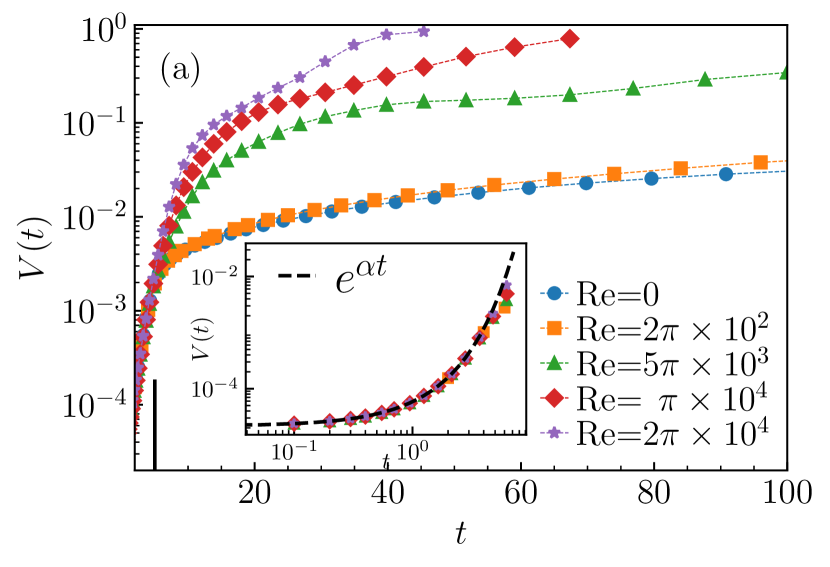
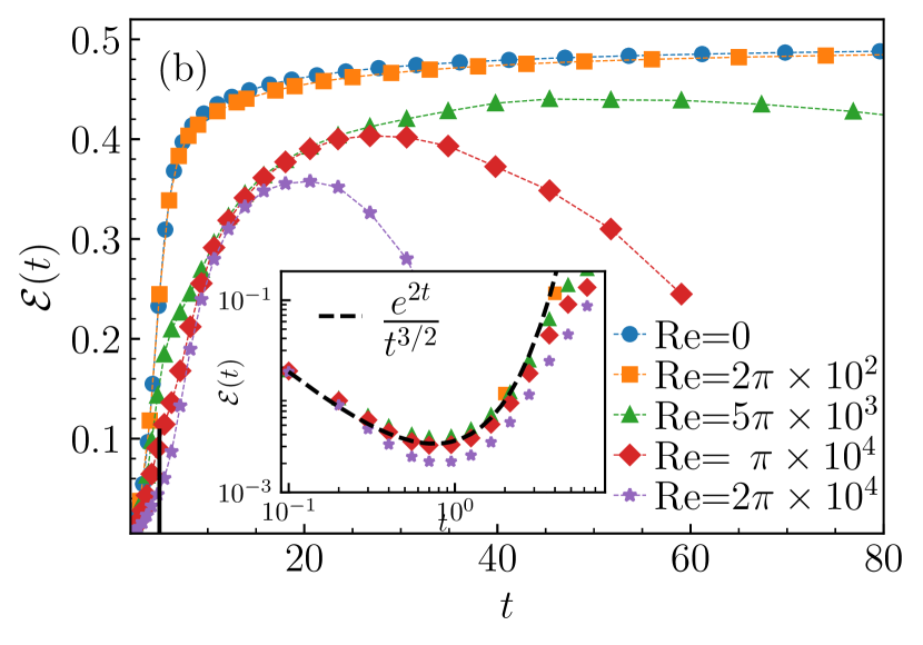
Figure 1: Time evolution of (a) $V(t)$ and (b) ${\mathcal{E}}(t)$ for different Re. (Insets) Zoomed in plots showing early time-evolution along with the theoretical prediction (dashed line).

At early times, the nonlinearities in Eq. 1 can be ignored and we arrive at the following time evolution equation of the energy spectrum Bratanov et al. (2015); Rana and Perlekar (2020)

$$\partial_{t}E_{k}(t)\approx 2(\alpha-\nu k^{2})E_{k}(t).$$ (4)

Using Eq. 4 and the initial condition for the energy spectrum we obtain $V(t)\sim\exp(\alpha t)$ and ${\mathcal{E}}\sim\exp(2t)/t^{3/2}$ [see Fig. 1].

The departure from the early exponential growth of $V(t)$ and ${\mathcal{E}}(t)$ marks the onset of the phase-ordering regime. We observe that $V(t)$ approaches the ordered state faster by increasing the Reynolds number. On the other hand, ${\mathcal{E}}(t)$ first increases, attains a plateau and then decreases. The plateau region and the peak value of ${\mathcal{E}}(t)$ decrease with increasing Reynolds. Later we show that the width of the plateau region is related to strength of the energy cascade.

For the ITT equations, the excess free-energy per unit volume is $h\equiv\mbox{Cn}^{2}|\nabla\bm{u}|^{2}/2$ and the defects are identified as velocity nulls, i.e. spatial locations where $\bm{u}={\bm{0}}$. Since $n=D=3$ for us, the ITT equation permits unit magnitude topological charge. We locate defects using the algorithm prescribed by Berg and Lüscher (1981) that has been successfully used to study: (a) the role of defects in the 3D Heisenberg transition Lau and Dasgupta (1989), and (b) coarsening dynamics in the 3D Ginzburg-Landau equations Toyoki (1991). Similar algorithms have also been used to identify vector nulls in magnetohydrodynamics Greene (1990), and fluid turbulence Mora et al. (2021). In Fig. 2(a,b) we show the time evolution of the iso-$h$ surfaces overlaid with defect positions during phase-ordering for low and high-Re. The streamline plots of pair of oppositely charged defects undergoing merger are shown in Fig. 2(c) [$\mbox{Re}=0$] and Fig. 2(d) [$\mbox{Re}=2\pi\times 10^{4}$].

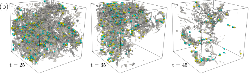
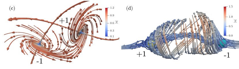
Figure 2: Iso-$h$ surfaces overlayed on the defect positions marked by colored spheres (blue : -1, yellow : +1) for (a) $\mbox{Re}=0$ and (b) $\mbox{Re}=\pi\times 10^{4}$ at different stages in the coarsening regime. We show only a subdomain of size $(\pi/2)^{3}$ from the simulation box for better visual representation. Streamlines of two neighbour defects undergoing merger at (c) $\mbox{Re}=0$ and (d) $\mbox{Re}=\pi\times 10^{3}$.

At low Re, in Fig. 2(a), we observe that the isosurfaces are primarily localized around the lines joining oppositely charged defects. The evolution resembles phase-ordering in the 3D Ginzburg-Landau equations Ostlund (1981); Toyoki (1991).

In contrast, at high-Re we find tubular structures similar to fluid turbulence Kaneda et al. (2003) and the defects reside in the proximity of these tubes [see Fig. 2(b)]. Furthermore, the visible clustering of defects at high-Re is consistent with the observed clustering of vector nulls in fluid turbulence Mora et al. (2021).

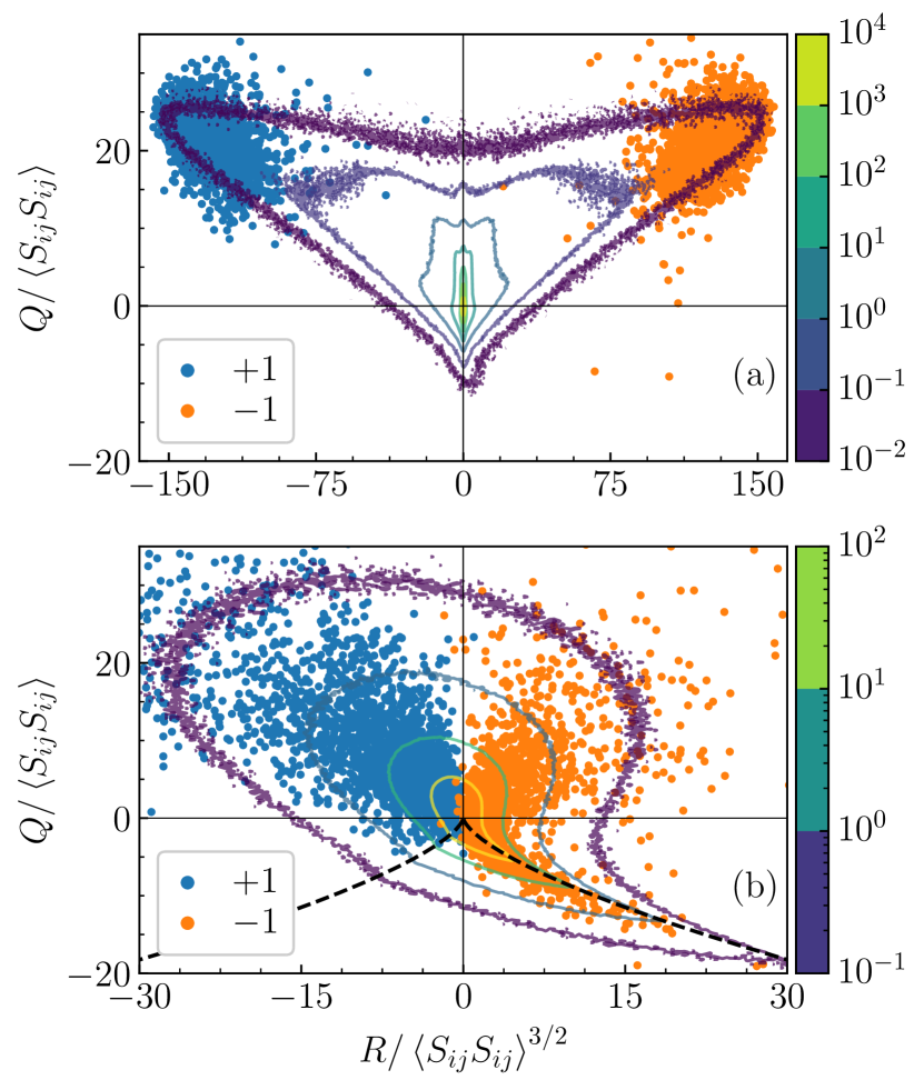
Figure 3: Contour plot of the joint probability distribution $P(R,Q)$ for (a) $\mbox{Re}=0$, and (b) $\mbox{Re}=\pi\times 10^{4}$ in the coarsening regime. Red (Blue) circles mark the position of +1(-1) defect on the $R-Q$ plane. In (b), the black dashed line shows the zero-discriminant curve $D\equiv 27R^{2}+4Q^{3}=0$ that distinguishes vortical ($D>0$) and strain-dominated ($D<0$) regions.

The spatial structures of fluid flows are often characterized by the invariants $Q\equiv-\mathrm{Tr}(\bm{A}^{2})/3$ and $R\equiv-\mathrm{Tr}(\bm{A}^{3})/3$ of the velocity gradient tensor $\bm{A}\equiv\nabla\bm{u}$. For high-Re fluid turbulence, the joint probability distribution function $P(R,Q)$ resembles an inverted tear-drop Pandit et al. (2009). In the R-Q plane, regions above the curve $(27/4)R^{2}+Q^{3}=0$ are vortical, whereas those below are extensional Ooi et al. (1999). From the flow structures around topological defects [see Fig. 2(c,d)], it is easy to identify that a positive (negative) topological charge would have $R<0(>0)$.

In Fig. 3, we plot the joint probability distribution function $P(R,Q)$ for $\mbox{Re}=0$ and $\mbox{Re}=2\pi\times 10^{4}$ at a representative time in the phase-ordering regime. By overlaying the $Q$ and $R$ values at the location of topological defects on the $P(R,Q)$, as expected, we find that the negative (positive) defects occupy the region with $R>0(<0)$. For $\mbox{Re}=0$, we find symmetric $P(R,Q)$ located primarily in the region $Q>0$, indicating that the flow structures are vortical. In contrast, for $\mbox{Re}=2\pi\times 10^{4}$ we observe that $P(R,Q)$ has a tear-drop shape reminiscent of fluid turbulence. The tail region ($Q>0$ and $R<0$) indicates strongly dissipative extensional flow regions (which also carry a negative charge).

A unique length scale typically describes the dynamics of systems undergoing phase-ordering, this is often referred to as the dynamic scaling hypothesis. In the following sections we investigate the validity of this hypothesis for phase-ordering in the ITT equation for low and high-Re.

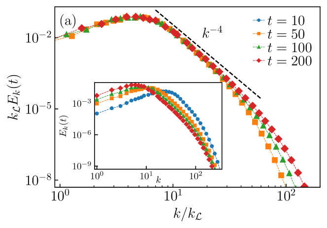
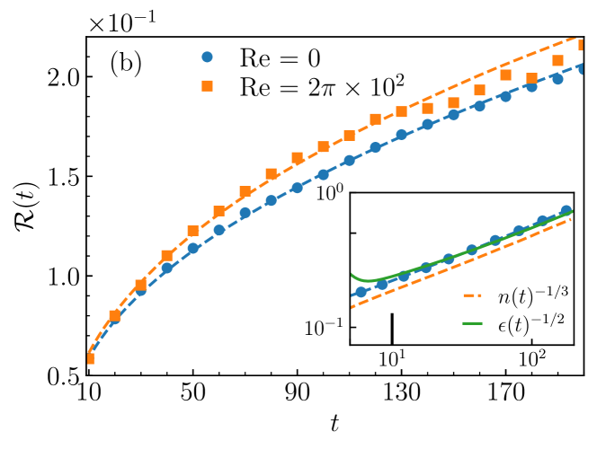
Figure 4: (a) Scaled energy spectrum $k_{\cal L}E_{k}(t)$ versus $k/k_{\cal L}$ for $\mbox{Re}=0$ at different times. For $k\ll k_{\mathcal{L}}$, we observe Porod’s scaling $E_{k}(k)\sim k^{-4}$. (Inset) Time evolution of the energy spectrum. (b) Evolution of average minimum inter-defect separation $R(t)$ for $\mbox{Re}=0$ and $\mbox{Re}=2\pi\times 10^{2}$. Dashed lines show the evolution of $\mathcal{L}(t)$ (scaled for comparison with $R(t)$). (Inset) Plot showing ${\mathcal{L}}(t)n(t)^{1/3}$ versus $t$ at $\mbox{Re}=0$.

Low Reynolds number– In Fig. 4, we plot the energy spectrum. With time, the peak of the spectrum shifts towards small-wave numbers, indicating a growing length scale often defined as Onuki (2002); Qian and Mazenko (2003); Bray (1993); Yurke et al. (1993); Mondello and Goldenfeld (1990); Onuki (2002); Rana and Perlekar (2020)

$${\mathcal{L}}(t)\equiv 2\pi\frac{\sum_{k}E_{k}(t)}{\sum_{k}kE_{k}(t)}.$$ (5)

For low $\mbox{Re}\to 0$, consistent with the Ginzburg-Landau scaling, we observe ${\mathcal{L}}(t)\sim\sqrt{t}$ [see Fig. 4(b)] Bray (2002). The rescaled energy spectrum $k_{\mathcal{L}}E_{k}$ versus $k/k_{\mathcal{L}}$ collapses onto a single curve for different times [see Fig. 4(a)], and we observe Porod’s scaling $E_{k{\mathcal{L}}}\propto(k{\mathcal{L}})^{-4}$ for $k{\mathcal{L}}(t)>1$ due to the presence of defects Bray (2002).

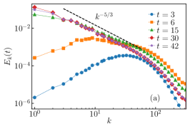
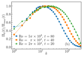
Figure 5: (a) Evolution of the energy spectrum at $\mbox{Re}=\pi\times 10^{4}$. Dashed black line shows the Kolmogorov scaling $k^{-5/3}$. (b) Energy flux at different Re in the coarsening regime. At higher Re, the wavenumber range over which we observe the energy flux increases. (c) Evolution of the maximum of energy flux $\Pi_{max}(t)$ at various Re.

Figure 6: Pseudocolor plot of the velocity magnitude (z=$\pi$ plane) along with the velocity streamlines during the late stages of phase-ordering for $\mbox{Re}=2\pi\times 10^{4}$.

The plot in Fig. 4(b) shows that the average minimum inter-defect separation $R(t)\propto{\mathcal{L}}(t)$, validating the dynamical scaling hypothesis. For uniformly distributed defects, we expect ${\mathcal{L}}(t)\propto n(t)^{-1/3}$, where $n(t)$ is the defect number density Chandrasekhar (1943); Hertz (1909); Rana and Perlekar (2020). We verify this in Fig. 4(b,inset).

High Reynolds number– In Fig. 5(a) we show the time evolution of the energy spectra for high $\mbox{Re}=5\pi\times 10^{3}$. At early times, similar to small Re, the peak of the spectrum shifts towards small $k$. At intermediate times which correspond to the plateau region in Fig. 2 (b), we observe a Kolmogorov scaling $E_{k}\sim k^{-5/3}$ [Fig. 5(b)]. A crucial feature of homogeneous, turbulence is the existence of a region of constant energy flux $\Pi_{k}\equiv\lambda\sum_{|\bm{p}|\leq|\bm{k}|}^{N/2}\widehat{\bm{u}}_{\bm{p}}\cdot(\widehat{\bm{u}\cdot\nabla\bm{u}})_{\bm{-p}}$ Frisch and Kolmogorov (1995). We evaluate $\Pi_{k}$ for different $\mbox{Re}=2\pi\times 10^{4}$ at representative times in the phase-ordering regime and find that it remains nearly constant between wave-numbers corresponding to the coarsening scale $k_{\mathcal{L}}\sim 2\pi/{\mathcal{L}}$ and the dissipation scale $k_{\eta}\sim(\nu^{3}/\Pi_{k})^{1/4}$ [Fig. 5(b)]. In Fig. 5(c), we show the time evolution of $\Pi_{max}(t)\equiv max[\Pi_{k}(t)]$. The time range over which $\Pi_{max}(t)$ is nearly constant coincides with the plateau region in ${\mathcal{E}}(t)$. At high-Re, the strong turbulence–marked by a broader inertial range and higher magnitude of $\Pi_{max}$– leads to a faster ordering. On reducing the Re, the cascade range and its strength reduces, we observe a broader time-window over which $\Pi_{max}$ remains constant.

Thus the following picture of phase-ordering emerges: active driving $\alpha-\beta|\bm{u}|^{2}$ injects energy primarily at large length scales, which is then redistributed to small scales by a forward energy cascade due to the advective nonlinearity. At late times, we observe regions of turbulence interspersed with growing patches of order (Fig. 6).

To conclude, we study the coarsening dynamics of the 3D ITT equation. We find that similar to 2D, phase ordering proceeds via repeated defect merger Rana and Perlekar (2020). At low Re, the defects are uniformly distributed throughout the domain and the dynamics is characterized by a unique growing length scale. On the other hand, at high Re, defects are clustered and the advective nonlinearities controls the phase ordering. In particular, we observe the Kolmogorov scaling in the energy spectrum and a region of constant energy flux.