Optimal Eddy Viscosity in Closure Models for 2D Turbulent Flows

Abstract

We consider the question of fundamental limitations on the performance of eddy-viscosity closure models for turbulent flows, focusing on the Leith model for 2D Large-Eddy Simulation. Optimal eddy viscosities depending on the magnitude of the vorticity gradient are determined subject to minimum assumptions by solving PDE-constrained optimization problems defined such that the corresponding optimal Large-Eddy Simulation best matches the filtered Direct Numerical Simulation. First, we consider pointwise match in the physical space and the main finding is that with a fixed cutoff wavenumber $k_{c}$, the performance of the Large-Eddy Simulation systematically improves as the regularization in the solution of the optimization problem is reduced and this is achieved with the optimal eddy viscosities exhibiting increasingly irregular behavior with rapid oscillations. Since the optimal eddy viscosities do not converge to a well-defined limit as the regularization vanishes, we conclude that in this case the problem of finding an optimal eddy viscosity does not in fact have a solution and is thus ill-posed. We argue that this observation is consistent with the physical intuition concerning closure problems. The second problem we consider involves matching time-averaged vorticity spectra over small wavenumbers. It is shown to be better behaved and to produce physically reasonable optimal eddy viscosities. We conclude that while better behaved and hence practically more useful eddy viscosities can be obtained with stronger regularization or by matching quantities defined in a statistical sense, the corresponding Large-Eddy Simulations will not achieve their theoretical performance limits.

I Introduction

The closure problem is arguably one of the most important outstanding open problems in turbulence research. It touches upon some of the key basic questions concerning turbulent flows and at the same time has far-reaching consequences for many applications, most importantly, for how we simulate turbulent flows in numerous geophysical, biological and engineering settings. Given the extreme spatio-temporal complexity of turbulent flows, accurate numerical solutions of the Navier-Stokes system even at modest Reynolds numbers requires resolutions exceeding the capability of commonly accessible computational resources. To get around this difficulty, one usually relies on various simplified versions of the Navier-Stokes system obtained through different forms of averaging and/or filtering, such as the Reynolds-Averaged Navier-Stokes (RANS) system and the Large-Eddy Simulation (LES). However, such formulations are not closed, because these systems involve nonlinear terms representing the effect of unresolved subgrid stresses on the resolved variables. The “closure problem” thus consists in expressing these quantities in terms of resolved variables such that the RANS or LES system is closed.

In general, closure models in fluid mechanics are of two main types: algebraic, where there is an algebraic relationship expressing the subgrid stresses in terms of the resolved quantities, and differential, where this relationship involves an additional partial-differential equation (PDE) which needs to be solved together with the RANS or LES system. Most classical models are usually formulated based on some ad-hoc, albeit well-justified, physical assumptions. There exists a vast body of literature concerning the design, calibration and performance of such models in various settings. Since it is impossible to offer an even cursory survey of these studies here, we refer the reader to the well-known monographs (Lesieur, 1993; Pope, 2000; Davidson, 2015) for an overview of the subject. Recently, there has been a lot of activity centered on learning new empirical closure models from data using methods of machine learning (Kutz, 2017; Gamahara and Hattori, 2017; Jimenez, 2018; Duraisamy et al., 2019; Duraisamy, 2021; Pawar and San, 2021). It is however fair to say that the field of turbulence modelling has been largely dominated by empiricism and there is a consensus that the potential and limitations of even the most common models are still not well understood. Our study tackles this fundamental question, more specifically, how well certain common closure models can in principle perform if they are calibrated in a optimal way. We will look for an optimal, in a mathematically precise sense, form of a certain closure model and will conclude that, somewhat surprisingly, it does not in fact exist.

On the other hand, from the physical point of view, turbulence closure models are not meant to capture nonlinear transfer processes with pointwise accuracy, but rather to represent them in a certain average sense. The ill-posedness of the problem of optimally calibrating a closure model signalled above can thus be viewed as a consequence of the inability of the closure model to match the original solution pointwise in space and in time. More precisely, the optimal eddy viscosity exhibits unphysical high-frequency oscillations. In the present study we will use a novel and mathematically systematic approach to illustrate this physical intuition and demonstrate how the ill-posedness arises. We will also show that the model calibration problem is in fact well-behaved when the LES with a closure model is required to match quantities defined in the statistical rather than pointwise sense.

We are going to focus on an example from a class of widely used algebraic closure models, namely, the Smagorinsky-type eddy-viscosity models (Smagorinsky, 1963) for LES. More specifically, we will consider the Leith model (Leith, 1968, 1971, 1996) for two-dimensional (2D) turbulent flows. Like all eddy-viscosity closure models, the Leith model depends on one key parameter which is the eddy viscosity typically taken to be a function of some flow variable. Needless to say, performance of such models critically depends on the form of this function. One specific question we are interested in is how accurately the LES equipped with such an eddy-viscosity closure model can at best reproduce solutions of the Navier-Stokes system obtained via Direct Numerical Simulation (DNS). Another related question we will consider concerns reproducing certain statistical properties of Navier-Stokes flows in LES. We will address these questions by formulating them as PDE-constrained optimization problems where we will seek an optimal functional dependence of the eddy viscosity on the state variable. In the first problem we will require the corresponding LES to match the filtered DNS pointwise in space over a time window of several eddy turnover times, whereas in the second problem the LES will be required to match the time-averaged enstrophy spectrum of the Navier-Stokes flow for small wavenumbers. By framing these questions in terms of optimization problems we will be able to find the best (in a mathematically precise sense) eddy viscosities, and this will in turn allow us to establish ultimate performance limitations for this class of closure models. We emphasize that the novelty of our approach is that by finding an optimal functional form of the eddy viscosity we identify, subject to minimum assumptions, an optimal structure of the nonlinearity in the closure model, which is fundamentally different, and arguably more involved, than calibrating one or more constants in a selected ansatz for the eddy viscosity. This formulation is also more general than common dynamic closure models and some formulations employing machine learning to deduce information about local properties of closure models from the DNS (see, e.g., (Maulik et al., 2020)). Our goal is to understand what form the eddy viscosity needs to take in order to maximize the performance of the closure model in achieving a prescribed objective. The emphasis will be on methodology rather than on specific contributions to subgrid modeling.

The optimization problem in question has a non-standard structure, but an elegant solution can be obtained using a generalization of the adjoint-based approach developed by Bukshtynov et al. (2011); Bukshtynov and Protas (2013). In being based on methods of the calculus of variations, this approach thus offers a mathematically rigorous alternative to machine-learning methods which have recently become popular (Kutz, 2017; Gamahara and Hattori, 2017; Jimenez, 2018; Duraisamy et al., 2019; Duraisamy, 2021; Pawar and San, 2021). As a proof of the concept applicable to the problem considered here, this approach was recently adapted to find optimal closures in a simple one-dimensional (1D) model problem by Matharu and Protas (2020). Importantly, this approach involves a regularization parameter controlling the “smoothness” of the obtained eddy viscosity.

In the first problem, which involves matching the filtered DNS solution in the pointwise sense, we find optimal eddy viscosities for the Leith closure model in the LES systems with different filter cutoff wavenumbers $k_{c}$. As this wavenumber increases and the filter width vanishes, the optimal eddy viscosity is close to zero and the match between the predictions of the LES and the filtered DNS is nearly exact, as expected. On the other hand, for smaller cutoff wavenumbers $k_{c}$ the optimal eddy viscosity becomes highly irregular whereas the match between the LES and DNS deteriorates, although it still remains much better than the match involving the LES with the standard Leith model or with no closure model at all. Interestingly, the optimal eddy viscosity reveals highly oscillatory behavior with alternating positive and negative values as the state variable increases. When the regularization in the solution of the optimization problems is reduced and the numerical resolution is refined at a fixed cutoff wavenumber, the frequency and amplitude of these oscillations are amplified which results in an improved match against the DNS. Thus, in this limit the optimal eddy viscosity becomes increasingly oscillatory as a function of the state variable which suggests that in the absence of regularization the problem of finding an optimal eddy viscosity does not in fact have a solution as the limiting eddy viscosity is not well defined. On the other hand, an arbitrarily regular eddy viscosity can be found when sufficient regularization is used in the solution of the optimization problem, but at the price of reducing the match against the DNS. While such smooth eddy viscosities may be more useful in practice, the corresponding LES models will not achieve their theoretical performance limits. In addition to this observation, our results also demonstrate how the best accuracy achievable by the LES with the considered closure model depends on the cutoff wavenumber of the filter, which sheds new light on the fundamental performance limitations inherent in this closure model.

In our second problem, which involves matching the time-averaged vorticity spectrum of the filtered DNS, the obtained optimal eddy viscosity is more regular and its key features remain essentially unchanged as the regularization in the solution of the optimization problems is reduced and the numerical resolution is refined. This demonstrates that the problem of optimally calibrating the closure model is better behaved when a suitable statistical quantity is used as the target. This is not surprising as such a formulation is in fact closer to the spirit of turbulence modelling.

The structure of the paper is as follows: in the next section we formulate our LES model and state the optimization problem defining the optimal eddy viscosity; in Section III we introduce an adjoint-based approach to the solution of the optimization problem and in Section IV discuss computational details; our results are presented in Section V whereas final conclusions are deferred to Section VI ; some additional technical material is provided in Appendix A.

II Large-Eddy Simulation and Optimal Eddy Viscosity

We consider 2D flows of viscous incompressible fluids on a periodic domain $\Omega:=[0,2\pi]^{2}$ over the time interval $[0,T]$ for some $T>0$ (“:=” means “equal to by definition”). Assuming the fluid is of uniform unit density $\rho=1$, its motion is governed by the Navier-Stokes system written here in the vorticity form

$$\partial_{t}{w}+\boldsymbol{\nabla}^{\perp}\psi\cdot\boldsymbol{\nabla}{w} =\nu_{N}\boldsymbol{\Delta}{w}-\alpha{w}+f_{\omega} \text{in}\quad{(0,T]\times\Omega},$$ (1a)

$$\boldsymbol{\Delta}\psi =-{w} \text{in}\quad{(0,T]\times\Omega},$$ (1b)

$${w}(t=0) ={w_{0}} \text{in}\quad\Omega,$$ (1c)

where $w=-\boldsymbol{\nabla}^{\perp}\cdot\boldsymbol{u}$, with $\boldsymbol{\nabla}^{\perp}=[\partial_{x_{2}},-\partial_{x_{1}}]^{T}$ and $\boldsymbol{u}$ the velocity field, is the vorticity component perpendicular to the plane of motion, $\psi$ is the streamfunction, $\nu_{N}$ is the coefficient of the kinematic viscosity (for simplicity, we reserve the symbol $\nu$ for the eddy viscosity), and ${w_{0}}$ is the initial condition. System (1) is subject to two forcing mechanisms: a time-independent forcing $f_{\omega}$ which ensures that the flow remains in a statistical equilibrium and the Ekman friction $-\alpha{w}$ describing large-scale dissipation due to, for example, interactions with boundary layers arising in geophysical fluid phenomena. The forcing term is defined to act on Fourier components of the solution with wavenumbers in the range $[k_{a},k_{b}]$ for some $0<k_{a}<k_{b}<\infty$, i.e.,

$$\left[\widehat{f}_{\omega}\right]_{\boldsymbol{k}}:=\begin{cases}F,\quad&k_{a}\leq|\boldsymbol{k}|\leq k_{b},\\ 0,\quad&\text{otherwise},\end{cases}$$ (2)

where $\left[\widehat{f}_{\omega}\right]_{\boldsymbol{k}}$ is the Fourier component of $f_{\omega}$ with the wavevector $\boldsymbol{k}$ (hereafter hats “ $\widehat{\cdot}$ ” will denote Fourier coefficients) and $F>0$ is a constant parameter.

The phenomenology of 2D forced turbulence is described by the Kraichnan-Batchelor-Leith theory (Kraichnan, 1967; Batchelor, 1969; Leith, 1968) which makes predictions about various physical characteristics of such flows. Their prominent feature, distinct from turbulent flows in three dimensions (3D), is the presence of a forward enstrophy cascade and an inverse energy cascade (Boffetta, 2007; Boffetta and Musacchio, 2010; Bracco and McWilliams, 2010; Vallgren and Lindborg, 2011; Boffetta and Ecke, 2012). Here we will chose $k_{a}$ and $k_{b}$ such that the forcing term (2) will act on a narrow band of Fourier coefficients to produce a well-developed enstrophy cascade towards large wavenumbers and a rudimentary energy cascade towards small wavenumbers. The parameters $\nu_{N}$, $\alpha$ and $F$ will be adjusted to yield a statistically steady state with enstrophy $\mathcal{E}(t):=\int_{\Omega}{w}^{2}(t,\mathbf{x})\,d\Omega$ fluctuating around a well-defined mean value $\mathcal{E}_{0}$. The initial condition $\omega_{0}$ in 1c will be chosen such that the evolution begins already in this statistically steady state at time $t=0$.

II.1 The Leith Closure Model

The LES is obtained by applying a suitable low-pass filter $G_{\delta}$, where $\delta>0$ is its width, to the Navier-Stokes system (1) and defining the filtered variables ${\widetilde{w}}=G_{\delta}\ast{w}$ and $\widetilde{\psi}=G_{\delta}\ast\psi$ (“ $\ast$ ” denotes the convolution operation and hereafter we will use tilde “ $\widetilde{\cdot}$ ” to represent filtered variables). For simplicity, we will employ a sharp low-pass spectral filter defined in terms of its Fourier-space representation as

$$\left[\widehat{G}_{\delta}\right]_{\boldsymbol{k}}:=\begin{cases}1,&|\boldsymbol{k}|\leq{k_{c}},\\ 0,&\text{otherwise},\end{cases}$$ (3)

where ${k_{c}}$ is the largest resolved wavenumber such that the filter width is $\delta=2\pi/{k_{c}}$. Since we normally have $k_{b}<{k_{c}}$, it follows that $\widetilde{f_{\omega}}=f_{\omega}$. Application of filter (3) to the vorticity equation (1a) yields $\partial_{t}{\widetilde{w}}+{\stackon[-8pt]{$\boldsymbol{\nabla}^{\perp}\widetilde{\psi}\cdot\boldsymbol{\nabla}{\widetilde{w}}$}{\vstretch{1.3}{\hstretch{2.4}{\widetilde{\phantom{\;\;\;\;\;\;\;}}}}}}=\nu_{N}\boldsymbol{\Delta}{\widetilde{w}}-\alpha{\widetilde{w}}+f_{\omega}+M$, where the term $M$ represents the effect of the unresolved subgrid quantities

$$M={\stackon[-8pt]{\boldsymbol{\nabla}^{\perp}\widetilde{\psi}\cdot\boldsymbol{\nabla}{\widetilde{w}}}{\vstretch{1.3}{\hstretch{2.4}{\widetilde{\phantom{\;\;\;\;\;\;\;}}}}}-\stackon[-8pt]{\boldsymbol{\nabla}^{\perp}\psi\cdot\boldsymbol{\nabla}{w}}{\vstretch{1.3}{\hstretch{2.4}{\widetilde{\phantom{\;\;\;\;\;\;\;}}}}}}.$$ (4)

Since expression (4) depends on the original unfiltered variables ${w}$ and $\psi$, to close the filtered system the term $M$ must be modelled in terms of an expression involving the filtered variables only. We will do this using the Leith model (Leith, 1968, 1971, 1996), which has a similar structure to the Smagorinsky model (Smagorinsky, 1963) widely used as a closure for 3D flows, but is derived considering the forward enstrophy cascade as the dominant mechanism in 2D turbulent flows. There is evidence for good performance of the Leith model in such flows (Graham and Ringler, 2013; Maulik and San, 2017). Its preferred form is

$$M\approx\widetilde{M}=\boldsymbol{\nabla}\cdot(\widetilde{{\nu_{L}}\boldsymbol{\nabla}\widetilde{\omega}}),$$ (5)

in which $\widetilde{\omega}$ is the solution to the LES system, cf. 8, and the eddy viscosity is assumed to be a linear function of the magnitude of the vorticity gradient, i.e.,

$$\nu_{L}(s):=(C_{L}\delta)^{3}\,\sqrt{s}\qquad\text{with}\quad s:=|\boldsymbol{\nabla}\widetilde{\omega}|^{2}\in\mathcal{I}:=[0,s_{\text{max}}],$$ (6)

where the Leith constant $C_{L}=1$ and $s_{\text{max}}>0$ is a sufficiently large number to be specified later. We will refer to $\mathcal{I}$ as the “state space” domain.

While in the original formulation of the Leith model the eddy viscosity is taken to be a linear function of $|\boldsymbol{\nabla}\widetilde{\omega}|$ as in (6) (Graham and Ringler, 2013; Maulik and San, 2017), here we consider a general dependence of the eddy viscosity on $|\boldsymbol{\nabla}\widetilde{\omega}|$ in the form

$$\nu(s)=\left[\nu_{L}(s)+\nu_{0}\right]\varphi\left(\frac{s}{s_{\text{max}}}\right),$$ (7)

where $\nu_{0}>0$ and $\varphi\;:\;[0,1]\rightarrow\mathbb{R}$ is a dimensionless function subject to some minimum only assumptions to be specified below. The parameter $\nu_{0}$ is introduced to allow the eddy viscosity $\nu(s)$ to take nonzero values at $s=0$, in contrast to Leith’s original model (6). We remark that defining the eddy viscosity in terms of such a function $\varphi$ ensures that ansatz (7) is dimensionally consistent. Making $\varphi$ and $\nu$ functions of $|\boldsymbol{\nabla}\widetilde{\omega}|^{2}$, rather than of $|\boldsymbol{\nabla}\widetilde{\omega}|$, in (7) will simplify subsequent calculations. We add that ansatz (7) is used here to illustrate the approach and in principle one could also consider other formulations parametrized by nondimensional functions. With the Leith model (5)–(7), the LES version of the 2D Navier-Stokes system (1) takes the form

$$\partial_{t}\widetilde{\omega}+{\stackon[-8pt]{$\boldsymbol{\nabla}^{\perp}\widetilde{\psi}\cdot\boldsymbol{\nabla}\widetilde{\omega}$}{\vstretch{1.3}{\hstretch{2.4}{\widetilde{\phantom{\;\;\;\;\;\;\;}}}}}} =\boldsymbol{\nabla}\cdot{\stackon[-8pt]{$\left(\left[\nu_{N}+\nu(s)\right]\boldsymbol{\nabla}\widetilde{\omega}\right)$}{\vstretch{1.3}{\hstretch{3.0}{\widetilde{\phantom{\;\;\;\;\;\;\;\;\;}}}}}}-\alpha\widetilde{\omega}+f_{\omega} \text{in}\quad{(0,T]\times\Omega},$$ (8a)

$$\boldsymbol{\Delta}\widetilde{\psi} =-\widetilde{\omega} \text{in}\quad{(0,T]\times\Omega},$$ (8b)

$$\widetilde{\omega}(t=0) =\widetilde{\omega}_{0}{:=}\widetilde{w}_{0} \text{in}\quad\Omega,$$ (8c)

where the initial condition is given as the filtered initial condition (1c) from the DNS system.

An equivalent form of equation (8a) can be obtained noting that with the form of the filter given in (3), the decomposition of the subgrid stresses (4) reduces to $M=\boldsymbol{\nabla}^{\perp}\widetilde{\psi}\cdot\boldsymbol{\nabla}\widetilde{\omega}-{\stackon[-8pt]{$\boldsymbol{\nabla}^{\perp}\psi\cdot\boldsymbol{\nabla}\omega$}{\vstretch{1.3}{\hstretch{2.4}{\widetilde{\phantom{\;\;\;\;\;\;\;}}}}}}$ (Pope, 2000). As a result, the advection term in (8a) can be replaced with $\boldsymbol{\nabla}^{\perp}\widetilde{\psi}\cdot\boldsymbol{\nabla}\widetilde{\omega}$. While our numerical solution will be based on (8a), this second form will facilitate the derivations presented in Section III. We will assume that for all times $t\in[0,T]$ the filtered vorticity field $\widetilde{\omega}$ is in the Sobolev space $H_{0}^{2}(\Omega)$ of zero-mean functions with square-integrable second derivatives (Adams and Fournier, 2003). We stress the distinction between the fields $w$, $\widetilde{w}$, $\widetilde{\omega}$ which represent, respectively, the solution of the DNS system 1, its filtered version and the solution of the LES system 8.

II.2 Optimization Formulation for Eddy Viscosity

We consider two formulations with the DNS field matched pointwise in space and in time, and in a certain statistical sense. First, the optimal eddy viscosity will be found as a minimizer of an error functional representing the mean-square error between observations of the filtered DNS, i.e., of the filtered solution $\widetilde{w}(t,\mathbf{x})$ of the Navier-Stokes system (1), and observations the corresponding prediction $\widetilde{\omega}(t,\mathbf{x};{\varphi})$ of the LES model (8) with eddy viscosity $\nu$. These observations are acquired at points $\mathbf{x}_{i}$, $i=1,\dots,M^{2}$, forming a uniform $M\times M$ grid in $\Omega$ with operators $H_{i}\;:\;{H^{2}}(\Omega)\longrightarrow\mathbb{R}$ defined as

$$\left(H_{i}{\widetilde{\omega}}\right)(t):=\int_{\Omega}\delta(\mathbf{x}-\mathbf{x}_{i}){\widetilde{\omega}}(t,\mathbf{x})\,d\Omega={\widetilde{\omega}}(t,\mathbf{x}_{i}),\quad i=1,\dots,M^{2},$$ (9)

where $\delta(\cdot)$ is the Dirac delta distribution and observations $\left(H_{i}\widetilde{\omega}({\varphi})\right)(t)$ of the LES solution are defined analogously (an integral representation of the observation operators will be convenient for the derivation of the solution approach for the optimization problem presented in Section III). The number of the observations points $M^{2}$ will be chosen such that $M\gtrapprox k_{c}$, i.e., the observations will resolve all flow features with wavenumbers slightly higher than the cutoff wavenumber $k_{c}$ in (3). The error functional then takes the form

$${\mathcal{J}_{1}}({{\varphi}}):=\frac{1}{2}\int_{0}^{T}\sum_{i=1}^{M^{2}}\left[\left(H_{i}{\widetilde{w}}\right)(t)-\left(H_{i}\widetilde{\omega}({\varphi})\right)(t)\right]^{2}\,dt,$$ (10)

and is understood as depending on the function $\varphi$ parametrizing the eddy viscosity $\nu=\nu(s)$ via ansatz (7).

In the second formulation, the optimal eddy viscosity will be found by minimizing the error between the time-averaged vorticity spectra in the filtered DNS and predicted by the LES. For simplicity and with a slight abuse of notation, we will treat the wavenumber $k$ as a continuous variable, i.e., we will assume that $\boldsymbol{k}\in\mathbb{R}^{2}$ rather than $\boldsymbol{k}\in\mathbb{Z}^{2}$; in the actual implementation one needs to account for the discrete nature of the wavevector $\boldsymbol{k}$. The vorticity spectrum predicted by the LES is then defined as

$$E_{\widetilde{\omega}}(t,k):=\frac{1}{2}\int_{\mathscr{C}(k)}|\widehat{\widetilde{\omega}}(t,\boldsymbol{k})|^{2}\,dS(\boldsymbol{k}),\qquad\forall t,k\geq 0,$$ (11)

where $\widehat{\widetilde{\omega}}(t,\boldsymbol{k})$ is the Fourier transform of $\widetilde{\omega}(t,\mathbf{x})$ and $\mathscr{C}(k):=\{\boldsymbol{k}\in\mathbb{R}^{2}:|\boldsymbol{k}|=k\}$ a circle with radius $k$ in the $2$D plane. The vorticity spectrum $E_{w}(t,k)$ in the (filtered) DNS is defined analogously. Denoting $[f]_{T}:=(1/T)\int_{0}^{T}f(t)\,dt$ the time average of a function $f\>:\;[0,T]\rightarrow\mathbb{R}$, the error functional is defined as

$${\mathcal{J}_{2}(\varphi):=\frac{1}{4}\int_{k=0}^{k_{c}}\left(\left[E_{\widetilde{\omega}}(\cdot,k;\varphi)\right]_{T}-\left[E_{w}(\cdot,k)\right]_{T}\right)^{2}\,dk,}$$ (12)

with matching performed up to the cutoff wavenumber $k_{c}$.

The form of equation (8a) suggests that $\nu=\nu(s)$, and hence also $\varphi=\varphi(s/s_{\text{max}})$, must be at least piecewise $C^{1}$ functions on $\mathcal{I}$ and $[0,1]$, respectively. However, as will become evident in Section III, our solution approach imposes some additional regularity requirements, namely, $\nu=\nu(s)$ needs to be piecewise $C^{2}$ on $\mathcal{I}$ with the first and third derivatives vanishing at $s=0,s_{\text{max}}$. Since gradient-based solution approaches to PDE-constrained optimization problems are preferably formulated in Hilbert spaces (Protas et al., 2004), we shall look for an optimal function $\varphi$ parametrizing the optimal eddy viscosity as an element of the following linear space which is a subspace of the Sobolev space $H^{2}(\mathcal{I})$

$$\mathcal{S}:={\left\{\varphi\in{C^{3}([0,1])}\>:\>\frac{d}{d\xi}\varphi(\xi)=\frac{d^{3}}{d\xi^{3}}\varphi(\xi)=0\ \text{at}\ \xi=0,1\right\}}.$$ (13)

Then, the problem of finding an optimal eddy viscosity in the two formulations becomes

$$\widecheck{\varphi}:=\underset{\varphi\in\mathcal{S}}{\operatorname*{arg\,min}}\,\mathcal{J}_{j}(\varphi),\qquad j=1,2,$$ (14)

where the optimal eddy viscosity $\widecheck{\nu}$ is deduced from $\widecheck{\varphi}$ via ansatz (7). Our approach to solving this problem is outlined in the next section.

III Adjoint-based Optimization

To fix attention, we focus here on solution of the optimization problem in the first formulation, i.e., for $j=1$ in (14), with the error functional given in (10). Essentially the same approach can also be used to solve the second optimization problem with the error functional (12) and required modifications are discussed in Appendix A. We formulate our approach in the continuous (“optimize-then-discretize”) setting (Gunzburger, 2003) and adopt the strategy developed and validated by Matharu and Protas (2020). Here we only summarize its key steps and refer the reader to that study for further details. A local solution of problem 10, 13–14 can be found using an iterative gradient-based minimization approach as $\widecheck{\varphi}=\underset{n\to\infty}{\text{lim}}\varphi^{(n)}$, where

$$\begin{cases}\varphi^{(n+1)}&=\varphi^{(n)}-\tau^{(n)}\,\nabla_{\varphi}\mathcal{J}_{1}(\varphi^{(n)}),\quad\quad n=0,1,\dots,\\ \varphi^{(0)}&=\varphi_{0},\end{cases}$$ (15)

in which $\varphi^{(n)}$ is the approximation of the optimal function $\widecheck{\varphi}$ at the $n$th iteration (which can be used to construct the corresponding approximation $\nu^{(n)}$ of the optimal eddy viscosity), $\nabla_{\varphi}\mathcal{J}_{1}(\varphi)$ is the gradient of the error functional (10) with respect to $\varphi$, $\tau^{(n)}$ is the step length along the descent direction and $\varphi_{0}$ is an initial guess usually suggested by some form of the eddy viscosity.

A central element of algorithm (15) is the gradient $\nabla_{\varphi}{\mathcal{J}_{1}}(\varphi)$. In many problems of PDE-constrained optimization it can be conveniently expressed using solutions of suitably-defined adjoint equations (Gunzburger, 2003). However, the present optimization problem 10, 13–14 has a nonstandard structure because the control variable $\varphi(s/s_{\text{max}})$ is a function of the dependent variable $s=|\boldsymbol{\nabla}\widetilde{\omega}|^{2}$ in system (8). On the other hand, in its standard formulation adjoint analysis allows one to obtain expressions for gradients depending on the independent variables in the problem (here, $t$ and $\mathbf{x}$). This difficulty was overcome by Bukshtynov et al. (2011); Bukshtynov and Protas (2013) who generalized adjoint analysis of PDE systems to problems of the type 10, 13–14 by introducing a suitable change of variables. For convenience we will denote $\sigma:=s/s_{\text{max}}$.

The Gâteaux (directional) differential of the error functional (10) with respect to ${{\varphi}}$, defined by ${\mathcal{J}_{1}}^{\prime}({{\varphi}};{\varphi}^{\prime}):=\lim_{\epsilon\to 0}\epsilon^{-1}\left[{\mathcal{J}_{1}}({{\varphi}}+\epsilon{\varphi}^{\prime})-{\mathcal{J}_{1}}({{\varphi}})\right]$, is defined as

$${\mathcal{J}_{1}}^{\prime}({{\varphi}};{\varphi}^{\prime})= \int_{0}^{T}\int_{\Omega}\,\sum_{i=1}^{M^{2}}H_{i}^{*}\left[\left(H_{i}\widetilde{\omega}({\varphi})\right)(t)-\left(H_{i}{\widetilde{w}}\right)(t)\right]\,{\widetilde{\omega}^{\prime}}(t,\mathbf{x};{{\varphi}},{\varphi}^{\prime})\,d\mathbf{x}\,dt,$$ (16)

where ${\varphi}^{\prime}\in\mathcal{S}$ is an arbitrary perturbation of the control variable ${\varphi}$, $\widetilde{\omega}^{\prime}(t,\mathbf{x};{{\varphi}},{\varphi}^{\prime})$ satisfies the system

$$\mathcal{K}\begin{bmatrix}\widetilde{\omega}^{\prime}\\ \\ \widetilde{\psi}^{\prime}\end{bmatrix}:=\begin{bmatrix}\partial_{t}\widetilde{\omega}^{\prime}+\boldsymbol{\nabla}^{\perp}\widetilde{\psi}^{\prime}\cdot\boldsymbol{\nabla}\widetilde{\omega}+\boldsymbol{\nabla}^{\perp}\widetilde{\psi}\cdot\boldsymbol{\nabla}\widetilde{\omega}^{\prime}+\alpha\widetilde{\omega}^{\prime}\qquad\qquad\qquad\\ -\boldsymbol{\nabla}\cdot\left(2(\boldsymbol{\nabla}\widetilde{\omega}\cdot\boldsymbol{\nabla}\widetilde{\omega}^{\prime})(\frac{d\nu}{d{s}}\,\varphi\boldsymbol{\nabla}\widetilde{\omega}+\frac{\nu_{L}+\nu_{0}}{s_{\text{max}}}\,\frac{d\varphi}{d\sigma}\,{\boldsymbol{\nabla}\widetilde{\omega}})+(\nu_{N}+\nu)\boldsymbol{\nabla}\widetilde{\omega}^{\prime}\right)\\ \boldsymbol{\Delta}\widetilde{\psi}^{\prime}+\widetilde{\omega}^{\prime}\end{bmatrix}=\begin{bmatrix}\boldsymbol{\nabla}\cdot\left((\nu_{L}+\nu_{0}){\varphi}^{\prime}\boldsymbol{\nabla}\widetilde{\omega}\right)\\ \\ 0\end{bmatrix},$$ (17a)

$$\widetilde{\omega}^{\prime}({t=0,\mathbf{x}})=0,$$ (17b)

obtained as linearization of the LES system 8 and $H_{i}^{*}\;:\;\mathbb{R}\longrightarrow{H^{-2}}(\Omega)$, $i=1,\dots,M^{2}$, are the adjoints of the observation operators $H_{i}$, cf. 9, given by

$${\forall\xi\in\mathbb{R},\qquad\left(H_{i}^{*}\xi\right):=\delta(\mathbf{x}-\mathbf{x}_{i})\xi,}\quad i=1,\dots,M^{2}.$$ (18)

In order to extract the gradient $\nabla_{{\varphi}}{\mathcal{J}_{1}}$ from the Gâteaux differential (16), we note that this derivative is a bounded linear functional when viewed as a function of ${\varphi}^{\prime}$ and invoke the Riesz representation theorem (Berger, 1977) to obtain

$${\mathcal{J}_{1}}^{\prime}({{\varphi}};{\varphi}^{\prime})=\left\langle\nabla_{{\varphi}}^{H^{2}}{\mathcal{J}_{1}},{\varphi}^{\prime}\right\rangle_{H^{2}({[0,1]})}=\left\langle\nabla_{{\varphi}}^{L^{2}}{\mathcal{J}_{1}},{\varphi}^{\prime}\right\rangle_{L^{2}({[0,1]})},$$ (19)

where the inner product in the space $H^{2}({[0,1]})$ is defined as

$$\Big{\langle}p_{1},p_{2}\Big{\rangle}_{H^{2}({[0,1]})}=\int_{0}^{1}p_{1}\,p_{2}+\ell_{1}^{2}\,\frac{dp_{1}}{d\sigma}\frac{dp_{2}}{d\sigma}+\ell_{2}^{4}\,\frac{d^{2}p_{1}}{d\sigma^{2}}\frac{d^{2}p_{2}}{d\sigma^{2}}\,d\sigma,$$ (20)

in which $\ell_{1}$ and $\ell_{2}$ are length-scale parameters. While for all values of $\ell_{1},\ell_{2}\in(0,\infty)$ the inner products (20) are equivalent (in the sense of norm equivalence), these two parameters play a very important role in regularization of solutions to the optimization problem (10)–(14). In 15 we require the gradient in the space $H^{2}({[0,1]})$, i.e., $\nabla_{{\varphi}}{\mathcal{J}_{1}}=\nabla_{{\varphi}}^{H^{2}}{\mathcal{J}_{1}}$, but it is convenient to first derive the gradient with respect to the $L^{2}$ topology.

Introducing adjoint fields $\widetilde{\omega}^{*}$ and $\widetilde{\psi}^{*}$, we can define the following duality-pairing relation

$$\left(\mathcal{K}\begin{bmatrix}\widetilde{\omega}^{\prime}\\ \widetilde{\psi}^{\prime}\end{bmatrix},\begin{bmatrix}\widetilde{\omega}^{*}\\ \psi^{*}\end{bmatrix}\right):= \int_{0}^{T}\int_{\Omega}\mathcal{K}\begin{bmatrix}\widetilde{\omega}^{\prime}\\ \widetilde{\psi}^{\prime}\end{bmatrix}\cdot\begin{bmatrix}\widetilde{\omega}^{*}\\ \widetilde{\psi}^{*}\end{bmatrix}\,d\mathbf{x}\,dt$$ (21)

$$\int_{0}^{T}\int_{\Omega}\begin{bmatrix}\widetilde{\omega}^{\prime}\\ \widetilde{\psi}^{\prime}\end{bmatrix}\cdot\mathcal{K}^{*}\begin{bmatrix}\widetilde{\omega}^{*}\\ \widetilde{\psi}^{*}\end{bmatrix}\,d\mathbf{x}\,dt=\left(\begin{bmatrix}\widetilde{\omega}^{\prime}\\ \widetilde{\psi}^{\prime}\end{bmatrix},\mathcal{K}^{*}\begin{bmatrix}\widetilde{\omega}^{*}\\ \psi^{*}\end{bmatrix}\right),$$

where integration by parts was performed with respect to both space and time (noting the periodic boundary conditions and the initial condition (17b)) and the adjoint system has the form

$$\mathcal{K}^{*}\begin{bmatrix}\widetilde{\omega}^{*}\\ \\ \widetilde{\psi}^{*}\end{bmatrix}:=\begin{bmatrix}-\partial_{t}\widetilde{\omega}^{*}-\boldsymbol{\nabla}^{\perp}\widetilde{\psi}\cdot\boldsymbol{\nabla}\widetilde{\omega}^{*}+\alpha\widetilde{\omega}^{*}+\widetilde{\psi}^{*}\qquad\qquad\qquad\qquad\\ -\boldsymbol{\nabla}\cdot\left(2\,(\boldsymbol{\nabla}\widetilde{\omega}\cdot\boldsymbol{\nabla}\widetilde{\omega}^{*})\,(\frac{d\nu}{d{s}}\,\varphi\boldsymbol{\nabla}\widetilde{\omega}+\frac{\nu_{L}+\nu_{0}}{s_{\text{max}}}\,\frac{d\varphi}{d\sigma}\,{\boldsymbol{\nabla}\widetilde{\omega}})+(\nu_{N}+\nu)\boldsymbol{\nabla}\widetilde{\omega}^{*}\right)\\ \boldsymbol{\Delta}\widetilde{\psi}^{*}-\boldsymbol{\nabla}^{\perp}\cdot(\widetilde{\omega}^{*}\,\boldsymbol{\nabla}\widetilde{\omega})\end{bmatrix}=\begin{bmatrix}W\\ \\ 0\end{bmatrix},$$ (22a)

$$\widetilde{\omega}^{*}({t=T,\mathbf{x}})=0,$$ (22b)

with the source term $W(t,\mathbf{x}):=\sum_{i=1}^{M^{2}}H_{i}^{*}\left[\left(H_{i}\widetilde{\omega}({\varphi})\right)(t)-\left(H_{i}{\widetilde{w}}\right)(t)\right]$. Combining (17), (21) and (22), we then arrive at

$$\left(\begin{bmatrix}\widetilde{\omega}^{\prime}\\ \widetilde{\psi}^{\prime}\end{bmatrix},\mathcal{K}^{*}\begin{bmatrix}\widetilde{\omega}^{*}\\ \widetilde{\psi}^{*}\end{bmatrix}\right) =\overbrace{\int_{0}^{T}\int_{\Omega}\,{W(t,\mathbf{x})}\,\widetilde{\omega}^{\prime}\,d\mathbf{x}dt}^{{\mathcal{J}_{1}}^{\prime}({{\varphi}};{\varphi}^{\prime})}$$ (23)

$$={-\int_{0}^{T}\int_{\Omega}\,\left(\nu_{L}+\nu_{0}\right)\,\left(\boldsymbol{\nabla}\widetilde{\omega}\cdot\boldsymbol{\nabla}\widetilde{\omega}^{*}\right)\,{\varphi}^{\prime}\,d\mathbf{x}\,dt,}$$

from which we obtain an expression for the Gâteaux differential

$${{\mathcal{J}_{1}}^{\prime}({{\varphi}};{\varphi}^{\prime})=-\int_{0}^{T}\int_{\Omega}\,\left(\nu_{L}+\nu_{0}\right)\,\left(\boldsymbol{\nabla}\widetilde{\omega}\cdot\boldsymbol{\nabla}\widetilde{\omega}^{*}\right)\,{\varphi}^{\prime}\,d\mathbf{x}\,dt{,}}$$

with the perturbation ${\varphi}^{\prime}$ now appearing explicitly as a factor. However, this expression is still not consistent with the Riesz form (19), which requires integration with respect to $s$ over $[0,1]$. In order to perform the required change of variables, we make the substitution $\varphi^{\prime}(\boldsymbol{\nabla}\widetilde{\omega}\cdot\boldsymbol{\nabla}\widetilde{\omega})=\int_{0}^{1}\,\delta\left(\frac{\boldsymbol{\nabla}\widetilde{\omega}\cdot\boldsymbol{\nabla}\widetilde{\omega}}{s_{\text{max}}}-\sigma\right)\,\varphi^{\prime}(\sigma)\,d\sigma$. Fubini’s theorem then allows us to swap the order of integration such that the Gâteaux differential (16) is finally recast in the Riesz form (19) as an integral with respect to $\sigma$

$${\mathcal{J}_{1}}^{\prime}({\varphi};\varphi^{\prime})=\int_{0}^{1}\left[-\int_{0}^{T}\int_{\Omega}\,\delta\left(\frac{\boldsymbol{\nabla}\widetilde{\omega}\cdot\boldsymbol{\nabla}\widetilde{\omega}}{s_{\text{max}}}-\sigma\right)\,\left(\nu_{L}+\nu_{0}\right)\,\boldsymbol{\nabla}\widetilde{\omega}\cdot\boldsymbol{\nabla}\widetilde{\omega}^{*}\,d\mathbf{x}\,dt\right]\,\varphi^{\prime}(\sigma)\,d\sigma.$$ (24)

The gradient defined with respect to the $L^{2}$ topology is then deduced from this expression as

$$\nabla_{\varphi}^{L^{2}}{\mathcal{J}_{1}}(\sigma)=-\int_{0}^{T}\int_{\Omega}\,\delta\left(\frac{\boldsymbol{\nabla}\widetilde{\omega}\cdot\boldsymbol{\nabla}\widetilde{\omega}}{s_{\text{max}}}-\sigma\right)\,\left(\nu_{L}+\nu_{0}\right)\,\boldsymbol{\nabla}\widetilde{\omega}\cdot\boldsymbol{\nabla}\widetilde{\omega}^{*}\,d\mathbf{x}\,dt.$$ (25)

The $L^{2}$ gradient given in (25) may in principle be discontinuous as a function of $s$ and hence will not ensure the regularity required of the optimal eddy viscosity, cf. Section II.2. To circumvent this problem, we define a Sobolev gradient using the Riesz relations (19) to identify the $H^{2}$ inner product (20) with expression (24) for the Gâteaux differential. Integrating by parts with respect to $\sigma$ and noting that the perturbation ${\varphi}^{\prime}\in\mathcal{S}$ is arbitrary, we obtain the Sobolev gradient $\nabla_{{\varphi}}^{H^{2}}{\mathcal{J}}$ as a solution of the elliptic boundary-value problem

$$\left[\operatorname{Id}-\ell_{1}^{2}\,\frac{d^{2}}{d\sigma^{2}}+\ell_{2}^{4}\frac{d^{4}}{d\sigma^{4}}\right]\nabla_{\varphi}^{H^{2}}\mathcal{J}_{1}(\sigma) =\nabla_{\varphi}^{L^{2}}\mathcal{J}_{1}(\sigma),\qquad\sigma\in[0,1],$$ (26a)

$$\frac{d^{(1)}\,(\nabla_{\varphi}^{H^{2}}\mathcal{J}_{1})}{d\sigma^{(1)}}\Big{|}_{\sigma=0,1} =\frac{d^{(3)}\,(\nabla_{\varphi}^{H^{2}}\mathcal{J}_{1})}{d\sigma^{(3)}}\Big{|}_{\sigma=0,1}=0.$$ (26b)

The choice of the boundary conditions in (26b) ensures the vanishing of all the boundary terms resulting from the integration by parts. There is in fact some freedom in how to cancel these terms and the choice in (26b) is arguably the least restrictive. As argued in Section II.1, we allow the eddy viscosity $\nu(s)$ to take nonzero values at $s=0$ so the corresponding Sobolev gradient should not vanish at $\sigma=0$ such that it can modify the value of $\varphi(0)$, which turns out to be important in practice, cf. Section V. Thus, the choice of boundary conditions at $\sigma=0$ provided in (26b) is necessary. On the other hand, the choice of the boundary conditions at $\sigma=1$ has been found to have little effect on the gradient and on the obtained results provided $s_{\text{max}}$ is sufficiently large. Therefore, the form of these boundary conditions given in (26b) is justified by simplicity. The boundary conditions (26b) are the reason for the presence of additional constraints in the definition of space $\mathcal{S}$ in (13).

Determination of the Sobolev gradients $\nabla_{{\varphi}}^{H^{2}}\mathcal{J}_{1}$ based on the $L^{2}$ gradients $\nabla_{{\varphi}}^{L^{2}}{\mathcal{J}_{1}}$ by solving system (26) can be viewed as low-pass filtering of the latter gradient using a non-sharp filter (as discussed by Protas et al. (2004), this can be seen representing the operator $\left[\operatorname{Id}-\ell_{1}^{2}\,(d^{2}/d{\sigma}^{2})+\ell_{2}^{4}(d^{4}/d{\sigma}^{4})\right]^{-1}$ in the Fourier space). The parameters $\ell_{1}$ and $\ell_{2}$ serve as cutoff length scales representing the wavelengths of the finest features retained in the gradients $\nabla_{{\varphi}}^{H^{2}}{\mathcal{J}_{1}}$ such that increasing $\ell_{1}$ and $\ell_{2}$ has the effect of making the Sobolev gradient “smoother” and vice versa. Thus, $\ell_{1}$ and $\ell_{2}$ are “knobs” which can be tuned to control the regularity of the optimal eddy viscosities obtained as solutions of the problem (10)–(14).

Since by construction $\nabla_{{\varphi}}^{H^{2}}{\mathcal{J}_{1}}\in\mathcal{S}$, choosing the initial guess in (15) such that ${\varphi}_{0}\in\mathcal{S}$ will ensure that ${\varphi}^{(0)},{\varphi}^{(1)},\dots,{\widecheck{\varphi}}\in\mathcal{S}$. At each step in (15) an optimal step size $\tau^{(n)}$ can be found by solving the following line-minimization problem (Nocedal and Wright, 2006)

$$\tau^{(n)}=\operatorname*{arg\,min}_{\tau>0}{\mathcal{J}_{1}}({\varphi}^{(n)}-\tau\,\nabla_{{\varphi}}{\mathcal{J}_{1}}({\varphi}^{(n)})).$$ (27)

Numerical implementation of the approach outlined above is discussed in the next section.

IV Computational Approach

The evaluation of the Sobolev gradient $\nabla_{{\varphi}}^{H^{2}}{\mathcal{J}_{1}}$ requires the numerical solutions of the LES system 8 and the adjoint system 22 followed by the solution of problem 26. For the first two systems we use a standard Fourier pseudo-spectral method in combination with a CN/RKW3 time-stepping technique introduced by Le and Moin (1991) which give spectrally accurate results in space and a globally second-order accuracy in time. The spatial domain is discretized using $N_{x}=256$ equispaced grid points in each direction. Since the eddy viscosity $\nu=\nu(s)$ and the function $\varphi(s/s_{\text{max}})$ are state-dependent, we also need to discretize the state domain $\mathcal{I}$, cf. (7), which is done using $N_{s}$ Chebyshev points (values of $N_{s}$ are provided in Table 1). We use Chebyshev differentiation matrices to perform differentiation with respect to $s$ and the eddy viscosity $\nu(s)$ and its derivatives are interpolated from state space $\mathcal{I}$ to the spatial domain $\Omega$ using the barycentric formulas (Trefethen, 2013). The boundary-value problem (26) is solved using a method based on ultraspherical polynomials available in the chebop feature of Chebfun (Driscoll et al., 2014). Solution of the 2D Navier-Stokes system 1 is dealiased using Gaussian filtering based on the $3/2$ rule (Hou, 2009), however, this is unnecessary for the LES system 8 due to the aggressive filtering applied. To ensure that aliasing errors resulting from the presence of state-dependent viscosity are eliminated, the adjoint system 22 is solved using twice as many grid points $2N_{x}$ in each direction.

Evaluation of the $L^{2}$ gradient 25 requires non-standard integration over level sets as described by Bukshtynov and Protas (2013). While for simplicity a simple gradient approach was presented in (15), in practice we use the Polak-Ribière variant of the conjugate-gradient method to accelerate convergence. For the line minimization problem 27, the standard Brent’s algorithm is used (Press et al., 2007). The consistency and accuracy of the formulation and of the entire computational approach was validated using a standard suite of tests as was done by Matharu and Protas (2020).

V Results

The results obtained by solving optimization problem (14) with error functionals 10 and 12 are presented in Sections V.1 and V.2 below. Our computations are based on a flow problem defined by the following parameters $\nu_{N}=1\times 10^{-2}$, $\alpha=1\times 10^{-3}$, $F=5$, and $k_{a}=k_{b}=4$. In the first optimization problem we fix $M=32$ in (10), which is slightly larger than the largest cutoff wavenumber $k_{c}$ we consider (cf. Table 1) and therefore ensures that the optimal eddy viscosity is determined based on all available flow information, and $T=20\approx 30t_{e}$, where $t_{e}:=\left[\int_{0}^{T}\mathcal{E}(t)\,dt/(8\pi^{2}T)\right]^{-1/2}$ is the eddy turnover time (Bracco and McWilliams, 2010). We emphasize that the key insights provided by our computations do not depend on the particular choice of $T$, as long as it remains of comparable magnitude to the value given above.

V.1 Matching the DNS Pointwise in Space and Time — Results for the Optimization Problem with Error Functional (10)

Our first set of results addresses the effect of the cutoff wavenumber $k_{c}$. They are obtained by solving problem 14 with ${j}=1$ for decreasing values of $k_{c}=30,25,20$ while retaining fixed values of the regularization parameters $\ell_{1},\ell_{2}$ and a fixed resolution $N_{s}$ in the state space $\mathcal{I}$, cf. cases A, B and C in Table 1. In each case the optimization problem is solved using the initial guess $\varphi_{0}(s/s_{\text{max}})\equiv 0$ corresponding to no closure model at all. The dependence of the error functional ${\mathcal{J}_{1}}(\nu^{(n)})$ on iterations $n$ in the three cases is shown in Figure 1a, where we see that the mean-square errors between the DNS and the optimal LES increase as the cutoff wavenumber $k_{c}$ is decreased and the largest relative reduction of the error is achieved in case C with the smallest $k_{c}$. While minimization in problem (14) is performed with respect to the nondimensional function $\varphi$, cf. (7), we focus here on the corresponding optimal eddy viscosities $\widecheck{\nu}=\widecheck{\nu}(s)$ shown in Figure 1b. Since small values of $s$ are attained more frequently in the flow, cf. the probability density function (PDF) of $\sqrt{s}$ embedded in the figure, the horizontal axis is scaled as $\sqrt{s}$ which magnifies the region of small values of $s$. We see that for the largest cutoff wavenumber $k_{c}=30$ the optimal eddy viscosity is close to zero over the entire range of $s$. However, for decreasing $k_{c}$ the optimal eddy viscosity exhibits oscillations of increasing magnitude. We note that values of $s\gtrapprox 50$ occur very rarely in the flow and hence the gradient (25) provides little sensitivity information for $s$ in this range. Thus, the behavior of $\widecheck{\nu}(s)$ for $s\gtrapprox 50$ is an artifact of the regularization procedure defined in (26) and is not physically relevant.

Case	$k_{c}$	$N_{s}$	$\ell_{1}$	$\ell_{2}$	${\varphi}_{0}$	${\mathcal{J}_{1}}({\varphi}_{0})$	${\mathcal{J}_{1}}({\varphi}^{(\infty)})$	$r$
A	30	$64$	$10^{4}$	$10^{3}$	No Closure	$4.398\times 10^{-7}$	$1.492\times 10^{-7}$	$8.999\times 10^{-8}$
B	25	$64$	$10^{4}$	$10^{3}$	No Closure	$1.951\times 10^{-5}$	$2.450\times 10^{-6}$	$1.572\times 10^{-6}$
C	20	$64$	$10^{4}$	$10^{3}$	No Closure	$3.635\times 10^{-4}$	$6.217\times 10^{-5}$	$4.468\times 10^{-5}$
D	20	$128$	$10^{3}$	$10^{2}$	Case C	$6.217\times 10^{-5}$	$2.001\times 10^{-5}$	$1.239\times 10^{-5}$
E	20	$256$	$10^{1}$	$10^{0}$	Case D	$2.333\times 10^{-5}$	$1.450\times 10^{-5}$	$8.723\times 10^{-6}$

Table 1: Summary information about the different cases considered when solving optimization problem (14) with $j=1$.

In order to provide additional insights about the properties of the optimal eddy viscosity, our second set of results is obtained as solutions of problem 14 with ${j}=1$ using a fixed $k_{c}=20$ and progressively reduced regularization achieved by decreasing the parameters $\ell_{1},\ell_{2}$ while simultaneously refining the resolution $N_{s}$ in the state space $\mathcal{I}$, cf. cases C, D and E in Table 1. Optimization problems with weaker regularization are solved using the optimal eddy viscosity obtained with stronger regularization as the initial guess. From the normalized error functionals shown as functions of iterations in Figure 2a, we see that as regularization is reduced, the mean-square errors between the optimal LES and the DNS become smaller and approach a certain nonzero limit, cf. Table 1. As is evident from Figure 2b, this is achieved with the corresponding optimal eddy viscosities developing oscillations with an ever increasing frequency. More precisely, each time the regularization parameters $\ell_{1},\ell_{2}$ are reduced and the resolution $N_{s}$ is refined, a new oscillation with a higher frequency appears in the optimal eddy viscosity $\widecheck{\nu}(s)$ (in fact, in each case, this is the highest-frequency oscillation which can be represented on a grid with $N_{s}$ points).

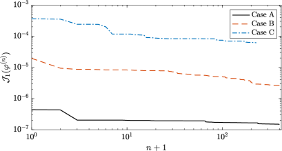
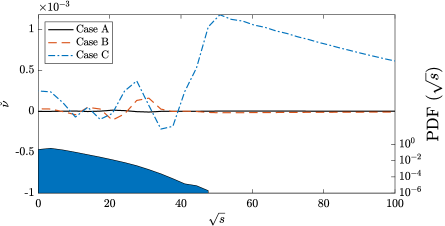
Figure 1: (a) Dependence of the functional ${\mathcal{J}_{1}}({\varphi}^{(n)})$ on the iteration $n$ and (b) dependence of the corresponding optimal eddy viscosity $\widecheck{\nu}$ on $\sqrt{s}$ for cases A, B and C, cf. Table 1. Panel (b) also shows the PDF of $\sqrt{s}$ in case C.

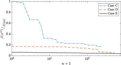
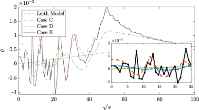
Figure 2: (a) Dependence of the normalized functional ${\mathcal{J}_{1}}({\varphi}^{(n)})/{\mathcal{J}_{1}}({\varphi}_{0})$, with ${\mathcal{J}_{1}}({\varphi}_{0})$ from case C, on the iteration $n$ and (b) dependence of the corresponding optimal eddy viscosity $\widecheck{\nu}$ on $\sqrt{s}$ for cases C, D and E, cf. Table 1. The inset in panel (b) shows magnification of the region $\sqrt{s}\in[0,25]$. Panel (b) also shows the Leith model with $k_{c}=20$ and the eddy viscosity $\nu_{L}(s)$, cf. (6).

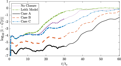
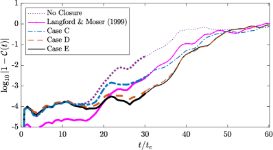
Figure 3: Adjusted normalized correlations 28 for the LES with (a) no closure and the optimal eddy viscosity in cases A, B and C, and (b) no closure and the optimal eddy viscosity in cases C, D and E. The correlation is also shown for the Leith model with $k_{c}=20$ and the eddy viscosity $\nu_{L}(s)$, cf. (6), in (a) and for an optimal closure model based on the stochastic estimator (Langford and Moser, 1999) in (b). Thick and thin lines correspond to, respectively, time in the “training window” ($t\in[0,T]$) and beyond this window ($t\in(T,2T]$).

In order to assess how well the solutions of the LES system (8) with the optimal eddy viscosities $\widecheck{\nu}$ shown in Figures 1b and 2b approximate the solution of the Navier-Stokes system (1), in Figures 3a and 3b we show the time evolution of the quantity $\log_{10}|1-\mathcal{C}(t)|$ where

$$\mathcal{C}(t):=\frac{1}{||\widetilde{w}(t)||_{L^{2}(\Omega)}\,||\widetilde{\omega}(t)||_{L^{2}(\Omega)}}\int_{\Omega}\widetilde{w}(t,\mathbf{x})\,\widetilde{\omega}(t,\mathbf{x})\ d\Omega$$ (28)

is the normalized correlation between the two flows. For a more comprehensive assessment, these results are shown for $t\in[0,2T]$, i.e., for times up to twice longer than the “training window” $[0,T]$ used in the optimization problem 14. In Figure 3b we also present the results obtained for $k_{c}=20$ with an optimal closure model based on the linear stochastic estimator introduced by Langford and Moser (1999). Since at early times correlation $\mathcal{C}(t)$ reveals exponential decay corresponding to the exponential divergence of the LES flow from the DNS, this effect can be quantified by approximating the correlation as $\mathcal{C}(t)\approx\bar{\mathcal{C}}(t):=\mathcal{C}_{0}e^{-rt}$, where $\mathcal{C}_{0}=1$ follows the fact that $\widetilde{\omega}_{0}\equiv\widetilde{w}_{0}$, whereas the decay rate $r$ is obtained from a least-squares fit over the time window $[0,T]$. The decay rates $r$ obtained in this way are collected in Table 1.

Finally, in order to provide insights about how the closure model with the optimal eddy viscosity acts in the physical space, in Figures 4a, 4b and 4d we show the vorticity field $\widetilde{\omega}(T,\mathbf{x})$, the corresponding state variable $s(T,\mathbf{x})$ cf. (7), and the spatial distribution $\widecheck{\nu}(s(T,\mathbf{x}))$ of the optimal eddy viscosity obtained in case E; for comparison, the spatial distribution of the eddy viscosity $\nu_{L}(s(T,\mathbf{x}))$ in the Leith model, cf. (6) with $\delta=0.02$, is shown in Figure 4c (the fields are shown in the entire domain, i.e., for $\mathbf{x}\in\Omega$, at the end of the training window). We see that while the vorticity and state-variable fields vary smoothly, this is also the case for the spatial distribution of the eddy viscosity $\nu_{L}(s(T,\mathbf{x}))$ in the Leith model. On the other hand, the spatial distribution of the optimal eddy viscosity $\widecheck{\nu}(s(T,\mathbf{x}))$ exhibits rapid variations, which is consistent with the results presented in Figure 2b. In particular, positive and negative values of $\widecheck{\nu}(s(T,\mathbf{x}))$, corresponding to localized dissipation and injection of enstrophy, tend to form concentric bands in some low-vorticity regions of the flow domain. The time evolution of the vorticity field in the DNS, LES with no closure model and LES with the optimal eddy viscosity (case E) are available together with an animated version of Figure 3b as a movie on-line. An animation representing the time evolution of the fields shown in Figure 4 for $t\in[0,{2}T]$ is available as a movie on-line.

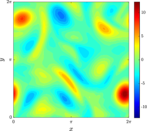
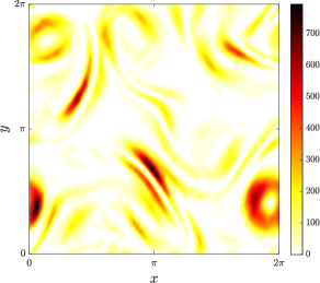
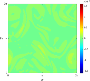
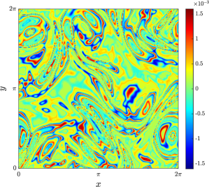
Figure 4: For case E we show: (a) the vorticity field $\widetilde{\omega}(T,\mathbf{x})$, $\mathbf{x}\in\Omega$, (b) the corresponding state variable $s(T,\mathbf{x})$, cf. (7), and the spatial distribution of (c) the eddy viscosity $\nu_{L}(s(T,\mathbf{x}))$ in the Leith model, cf. (6) with $\delta=0.02$, and (d) the optimal eddy viscosity $\widecheck{\nu}(s(T,\mathbf{x}))$, cf. Figure 2b, all shown at the end of the training window for $t=T$. For better comparison the same color scale is used in panels (c) and (d).

V.2 Matching the DNS in an Average Sense — Results for the Optimization Problem with Error Functional (12)

Now we review the results obtained by solving optimization problem (14) for ${j}=2$ with a fixed cutoff wavenumber $k_{c}=20$ and with two sets of parameters determining regularization ($\ell_{1}$ and $\ell_{2}$) and the resolution in the state space $\mathcal{I}$ ($N_{s}$), cf. cases F and G in Table 2. We remark that the regularization performed in the present problem is less aggressive than in the problem discussed in Section V.1. As shown in Figure 5a, the normalized error functional converges to a local minimum in only a few iterations and, as the regularization is reduced, a larger reduction of the error functional is obtained. However, as is evident from Figure 5b, this is achieved with optimal eddy viscosities much better behaved than the optimal eddy viscosities found by solving the optimization problem discussed in Section V.1, even though a weaker regularization is now applied, cf. Table 2 (the obtained optimal eddy viscosity exhibits more small-scale variability in case G than in case F, but the difference is not significant).

The difference between the time-averaged vorticity spectra (11) is the LES with no closure, LES with the optimal closure $\widecheck{\nu}$ (cases F and G) and in the filtered DNS is shown in Figure 6 as a function of the wavenumber $k$ (this quantity is related to the integrand expression in the error functional (12)). We see that when the optimal eddy viscosity $\widecheck{\nu}$ is used in the LES, this error is reduced, especially at low wavenumbers $k$. On the other hand, the evolution of the quantity $\log_{10}|1-\mathcal{C}(t)|$, cf. (28), shown for the same cases in Figure 7 demonstrates that, in contrast to Figure 3, in the present problem the LES flows equipped with the optimal eddy viscosity do not achieve a better pointwise-in-space accuracy with respect to the DNS than the LES flow with no closure model.

Finally, we show the vorticity field $\widetilde{\omega}(T,\mathbf{x})$, the corresponding state variable $s(T,\mathbf{x})$, cf. (7), the spatial distribution $\widecheck{\nu}(s(T,\mathbf{x}))$ of the optimal eddy viscosity obtained in case G, and for comparison, the spatial distribution of the eddy viscosity $\nu_{L}(s(T,\mathbf{x}))$ in the Leith model, cf. (6), in Figures 8a, 8b, 8d, and 8c, respectively. We remark that the spatial distribution of the optimal eddy viscosity in Figure 8d is now significantly smoother than the distribution of the optimal eddy viscosity obtained in the first formulation by solving optimization problem (14) with ${j}=1$, cf. Figure 4d. An animated version of Figure 8 illustrating the evolution of the fields for $t\in[0,{2}T]$ is available as a movie on-line.

Case	$k_{c}$	$N_{s}$	$\ell_{1}$	$\ell_{2}$	$\varphi_{0}$	$\mathcal{J}_{2}(\varphi_{0})$	$\mathcal{J}_{2}(\varphi^{(\infty)})$	$r$
F	20	$256$	$10^{1}$	$10^{0}$	No Closure	$6.736\times 10^{-2}$	$8.876\times 10^{-3}$	$2.882\times 10^{-4}$
G	20	$512$	$10^{-1}$	$10^{-2}$	No Closure	$6.736\times 10^{-2}$	$6.286\times 10^{-3}$	$1.685\times 10^{-4}$

Table 2: Summary information about the different cases considered when solving optimization problem (14) with ${j}=2$.

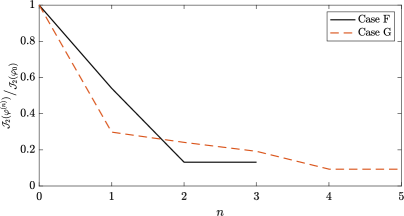
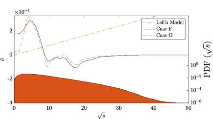
Figure 5: (a) Dependence of the normalized functional $\mathcal{J}_{2}({\varphi}^{(n)})/\mathcal{J}_{2}(\varphi_{0})$ on the iteration $n$ and (b) dependence of the corresponding optimal eddy viscosity $\widecheck{\nu}$ on $\sqrt{s}$ for cases F and G, cf. Table 2. Panel (b) also shows the PDF of $\sqrt{s}$ in case G.

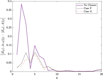
Figure 6: The difference between time-averaged vorticity spectra (11) in the filtered DNS and in the LES with no closure and with the optimal eddy viscosity $\widecheck{\nu}$ obtained in cases F and G, cf. Table 2, as function of the wavenumber $k$.

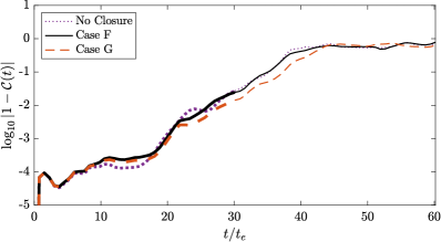
Figure 7: Adjusted normalized correlations 28 for the LES with no closure and the optimal eddy viscosity in cases F and G. Thick and thin lines correspond to, respectively, time in the “training window” ($t\in[0,T]$) and beyond this window ($t\in(T,2T]$).

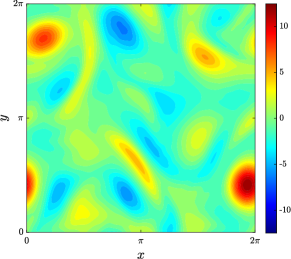
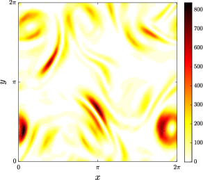
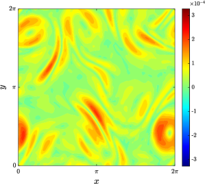
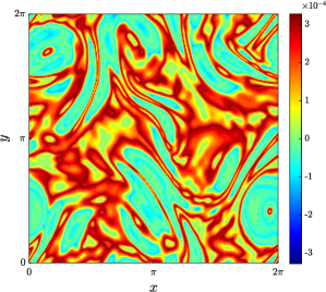
Figure 8: For case G we show: (a) the vorticity field $\widetilde{\omega}(T,\mathbf{x})$, $\mathbf{x}\in\Omega$, (b) the corresponding state variable $s(T,\mathbf{x})$, cf. (7), and the spatial distribution of (c) the eddy viscosity $\nu_{L}(s(T,\mathbf{x}))$ in the Leith model, cf. (6) with $\delta=0.02$, and (d) the optimal eddy viscosity $\widecheck{\nu}(s(T,\mathbf{x}))$, cf. Figure 5b, all shown at the end of the training window for $t=T$. For better comparison the same color scale is used in panels (c) and (d).

VI Discussion and Conclusions

In this study we have considered the question of fundamental limitations on the performance of eddy-viscosity closure models for turbulent flows. We focused on the Leith model for 2D LES for which we sought optimal eddy viscosities that subject to minimum assumptions would result in the least mean-square error between the corresponding LES and the filtered DNS. Such eddy viscosities were found as minimizers of a PDE-constrained optimization problem with a nonstandard structure which was solved using a suitably adapted adjoint-based gradient approach (Matharu and Protas, 2020). A key element of this approach was a regularization strategy involving the length-scale parameters $\ell_{1}$ and $\ell_{2}$ in the Sobolev gradients, cf. (26). The approach proposed is admittedly rather technically involved which may limit its practical applicability to construct new forms of the eddy viscosity, but its value is in making it possible to systematically characterize the best possible performance of different types of closure models.

Our main finding in Section V.1 is that with a fixed cutoff wavenumber $k_{c}$ the LES with an optimal eddy viscosity $\widecheck{\nu}$ matches the DNS increasingly well as the regularization in the solution of the optimization problem is reduced, cf. Figure 2a. This is quantified by a reduction of the rate of exponential decay of the correlation between the corresponding LES and the DNS, cf. Figure 3b and Table 1. This optimal performance of the closure model is achieved with eddy viscosities $\widecheck{\nu}(s)$ rapidly oscillating with a frequency increasing as the regularization parameters are reduced. From this we conclude that in the limit of vanishing regularization parameters and an infinite numerical resolution the optimal eddy viscosity would be undefined as it would exhibit oscillations with an unbounded frequency. Thus, from the mathematical point of view, the problem of finding an optimal eddy viscosity in the absence of regularization is ill-posed. In practical terms, this means that the “best” eddy viscosity for the Leith model does not exist.

The optimal performance of the LES is realized by a rapid variation of the eddy viscosity $\widecheck{\nu}(s)$ which oscillates between positive and negative values as $s$ changes, cf. Figure 2b, resulting in the dissipation and injection of the enstrophy occurring in the physical domain in narrow alternating bands, cf. Figure 4d. We note that a somewhat similar behavior was also observed in (Maulik et al., 2020) where the authors used machine learning methods to determine pointwise estimates of eddy viscosity which exhibited oscillations between positive and negative values. This behavior can be understood in physical terms based on relations (4)–(5) which can be interpreted as defining the eddy viscosity in terms of the space- and time-dependent DNS field, but the problem is severely overdetermined. Thus, some form of relaxation is needed to determine $\nu$ and the proposed optimization approach with its inherent regularization strategy is one possibility.

In addition, the optimal eddy viscosities found here have the property that $\widecheck{\nu}(0)>0$, in contrast to what is typically assumed in the Leith model where $\nu(0)=0$ (Maulik and San, 2017). In contrast to the behavior observed in Figure 4d, standard eddy viscosity closure models are usually assumed to be strictly dissipative Rodi et al. (2013), which is reflected in the fact that the eddy viscosity is non-negative as in Figure 4c. We add that we have also considered finding optimal eddy viscosities by matching against the unfiltered DNS field, i.e., using $w(t,\mathbf{x})$ in the error functional (10) instead of $\widetilde{w(}t,\mathbf{x})$, however, this approach produced results very similar to the ones reported above. As is evident from Figure 3b, the performance of the LES with optimal eddy viscosities compares favourably to the LES with an optimal closure model proposed by Langford and Moser (1999) based on a stochastic estimator, which has a less restrictive structure than the Leith model.

The optimal eddy viscosities constructed in Section V.1 to maximize the pointwise match against the filtered DNS are unlikely to be useful in practice due to their highly irregular behaviour which is difficult to resolve using finite numerical precision. On the other hand, the second formulation studied in Section V.2 where optimal eddy viscosities were determined by matching predictions of the LES against the time-averaged vorticity spectrum of the DNS for small wavenumbers lead to a much better behaved optimization problem and produced results easier to interpret physically. In particular, the general form of the optimal eddy viscosity obtained in this case was found to have little dependence on regularization, cf. Figure 5b.

The main question left open by the results reported here is whether the optimal eddy viscosity for the Smagorinsky model in 3D turbulent flows would exhibit similar properties. It can be studied by solving an optimization problem analogous to (14), a task we will undertake in the near future. In addition, it is also interesting to analyze the optimal performance of other closure models using the framework developed here.

Appendix A Gradient of the Error Functional $\mathcal{J}_{2}$

Here we discuss computation of the gradients $\nabla^{L^{2}}_{\varphi}\mathcal{J}_{2}$ and $\nabla^{H^{2}}_{\varphi}\mathcal{J}_{2}$ of the error functional 12. The difference with respect to the formulation used in Section III is that functional (12) is defined in the Fourier space and we adopt with suitable modifications the approach developed in Farazmand et al. (2011). Proceeding as in Section III, we first compute the Gâteaux differential of the error functional 12 with respect to $\varphi$

$$\mathcal{J}_{2}^{\prime}(\varphi;\varphi^{\prime})={\frac{1}{2T}\int_{t=0}^{T}\int_{k=0}^{k_{c}}\bigg{(}\left[E_{\widetilde{\omega}}(\cdot,k;\varphi)\right]_{T}-\left[E_{w}(\cdot,k)\right]_{T}\bigg{)}\,\left(\int_{\mathscr{C}(k)}\widehat{\widetilde{\omega}}\overline{\widehat{\widetilde{\omega}}}^{\prime}+\overline{\widehat{\widetilde{\omega}}}\widehat{\widetilde{\omega}}^{\prime}\,dS(\boldsymbol{k})\right)dk\,dt,}$$ (29)

where $\overline{\cdot}$ denotes the complex conjugate and $\widehat{\widetilde{\omega}}^{\prime}$ is the Fourier transform of the solution $\widetilde{\omega}^{\prime}$ to 17. We note that the gradients $\nabla^{L^{2}}_{\varphi}\mathcal{J}_{2}$ and $\nabla^{H^{2}}_{\varphi}\mathcal{J}_{2}$ satisfy Riesz identities analogous to (19). Next we introduce new adjoint fields $\widetilde{\omega}^{*}$ and $\widetilde{\psi}^{*}$ assumed to satisfy the same adjoint system (22), but with a different source term $W$ whose form is to be determined. Utilizing Parseval’s identity and the fact that all fields are real-valued in physical space, we rewrite the duality relation (21) as

$$\left(\begin{bmatrix}[1.0]\widetilde{\omega}^{\prime}\\ \widetilde{\psi}^{\prime}\end{bmatrix},\mathcal{K}^{*}\begin{bmatrix}[1.0]\widetilde{\omega}^{*}\\ \widetilde{\psi}^{*}\end{bmatrix}\right) =\frac{1}{2}\left(\widehat{\begin{bmatrix}[1.0]\widetilde{\omega}^{\prime}\\ \widetilde{\psi}^{\prime}\end{bmatrix}},\widehat{\mathcal{K}^{*}\begin{bmatrix}[1.0]\widetilde{\omega}^{*}\\ \widetilde{\psi}^{*}\end{bmatrix}}\right)+\frac{1}{2}\overline{\left(\widehat{\begin{bmatrix}[1.0]\widetilde{\omega}^{\prime}\\ \widetilde{\psi}^{\prime}\end{bmatrix}},\widehat{\mathcal{K}^{*}\begin{bmatrix}[1.0]\widetilde{\omega}^{*}\\ \widetilde{\psi}^{*}\end{bmatrix}}\right)},$$ (30)

$$={\frac{1}{2T}\,\int_{t=0}^{T}\int_{k=0}^{k_{c}}\int_{\mathscr{C}(k)}\widehat{\left[\begin{smallmatrix}\widetilde{\omega}^{\prime}\\ \widetilde{\psi}^{\prime}\end{smallmatrix}\right]}\cdot\overline{\widehat{\mathcal{K}^{*}\left[\begin{smallmatrix}\widetilde{\omega}^{*}\\ \widetilde{\psi}^{*}\end{smallmatrix}\right]}}+\overline{\widehat{\left[\begin{smallmatrix}\widetilde{\omega}^{\prime}\\ \widetilde{\psi}^{\prime}\end{smallmatrix}\right]}}\cdot\widehat{\mathcal{K}^{*}\left[\begin{smallmatrix}\widetilde{\omega}^{*}\\ \widetilde{\psi}^{*}\end{smallmatrix}\right]}\,dS(\boldsymbol{k})\,dk\,dt.}$$

Combining (17), (21), (22), 29 and 30 results in

$$\left(\begin{bmatrix}\widetilde{\omega}^{\prime}\\ \widetilde{\psi}^{\prime}\end{bmatrix},\mathcal{K}^{*}\begin{bmatrix}\widetilde{\omega}^{*}\\ \widetilde{\psi}^{*}\end{bmatrix}\right)=\overbrace{{\frac{1}{2T}\int_{t=0}^{T}\int_{k=0}^{k_{c}}\bigg{(}\left[E_{\widetilde{\omega}}(\cdot,k;\varphi)\right]_{T}-\left[E_{w}(\cdot,k)\right]_{T}\bigg{)}\,\left(\int_{\mathscr{C}(k)}\widehat{\widetilde{\omega}}\overline{\widehat{\widetilde{\omega}}}^{\prime}+\overline{\widehat{\widetilde{\omega}}}\widehat{\widetilde{\omega}}^{\prime}\,dS(\boldsymbol{k})\right)dk\,dt,}}^{\mathcal{J}_{2}^{\prime}({{\varphi}};{\varphi}^{\prime})}$$

from which we deduce the form of the source term in the adjoint system as

$$\widehat{W}(t,\boldsymbol{k})=\left(\left[E_{\widetilde{\omega}}(\cdot,k;\varphi)\right]_{T}-\left[E_{w}(\cdot,k)\right]_{T}\right)\,\widehat{\widetilde{\omega}}(t,\boldsymbol{k}).$$ (31)

Once the adjoint system (22) with the source term (31) is solved, the $L^{2}$ gradient $\nabla_{\varphi}^{L^{2}}\mathcal{J}_{2}$ can be computed using expression (25). The Sobolev gradient $\nabla_{\varphi}^{H^{2}}\mathcal{J}_{2}$ is then obtained as discussed in Section III by solving system (26). In summary, the difference in the computation of the gradients of the error functionals $\mathcal{J}_{1}$ and $\mathcal{J}_{2}$ is confined to the form of the source term $W$ in the adjoint system (22).