Gromov-Hausdorff distance between filtered $A_{\infty}$ categories 1: Lagrangian Floer theory

Abstract.

In this paper we introduce and study a distance, Gromov-Hausdorff distance, which measures how two filtered $A_{\infty}$ categories are far away each other.

In symplectic geometry the author associated a filtered $A_{\infty}$ category, Fukaya category, to a finite set of Lagrangian submanifolds. The Gromov-Hausdorff distance then gives a new invariant of a finite set of Lagrangian submanifolds.

One can estimate it by the Hofer distance of Hamiltonian diffeomorphisms needed to send one Lagrangain submanifold to the other.

A motivation to introduce Gromov-Hausdorff distance is to obtain a certain completion of Fukaya category. If we have a sequence of sets of Lagrangian submanifolds, which is a Cauchy sequence in the sense of Hofer metric, then the associated filtered $A_{\infty}$ categories also form a Cauchy sequence in Gromov-Hausdorff distance. In this paper we develop a theory to obtain an inductive limit of such a sequence of filtered $A_{\infty}$ categories. In other words, we give an affirmative answer to [Fu5, Conjecture 15.34].

We can use this result to associate a filtered $A_{\infty}$ category to a finite set of Lagrangian submanifolds, without assuming transversality conditions between Lagrangian submanifolds.

The author believes that the story of Gromov-Hausdorff distance between filtered $A_{\infty}$ categories will play an important role in the study of homological Mirror symmetry over Novikov ring. Recently homological Mirror symmetry over Novikov field is much studied. However there is practically no study of homological Mirror symmetry over Novikov ring at this stage.

Feb., 2021

1. Introduction

Let $(X,\omega)$ be a symplectic manifold that is compact or tame. We consider a finite set $\mathbb{L}$ of relatively spin (embedded and compact) Lagrangian submanifolds. When we assume that, for $L,L^{\prime}\in\mathbb{L}$ with $L\neq L^{\prime}$, $L$ is transversal to $L^{\prime}$, we obtain a filtered $A_{\infty}$ category $\mathfrak{F}(\mathbb{L})$ whose object is a pair $(L,b)$ such that $L\in\mathbb{L}$ and $b$ is a bounding cochain of $L$ in the sense of [FOOO1, Definition 3.6.4]. ([AFOOO, Fu5].)

In this paper we introduce a way to measure how two filtered $A_{\infty}$ categories are close each other. It is an analogue of Gromov-Hausdorff distance [GLP] between metric spaces and we call it Gromov-Hausdorff distance between filtered $A_{\infty}$ categories. We denote by $d_{\rm GH}(\mathscr{C}_{1},\mathscr{C}_{2})$ the Gromov-Hausdorff distance between filtered $A_{\infty}$ categories $\mathscr{C}_{1}$ and $\mathscr{C}_{2}$. There are a few different versions of Gromov-Hausdorff distance. See Definitions 2.5, 2.17, 12.9, and 12.10.

Gromov-Hausdorff distance satisfies the triangle inequality. It is actually a pseudo-distance. Namely $d_{\rm GH}(\mathscr{C}_{1},\mathscr{C}_{2})=0$ may not imply that $\mathscr{C}_{1}$ is isomorphic to $\mathscr{C}_{2}$.

We prove (in Corollaries 2.21 and 12.15) that if $\mathbb{L}=\{L_{1},\dots,L_{K}\}$ is a finite set of relatively spin Lagrangian submanifolds which are mutually transversal and if $\varphi_{i}$, $i=1,\dots,K$ is a finite set of Hamiltonian diffeomorphisms then

$$d_{\rm GH}(\mathfrak{F}(L_{1},\dots,L_{K}),\mathfrak{F}(\varphi_{1}(L_{1}),\dots,\varphi_{K}(L_{K})))\leq\max\{d_{\rm Hof}({\rm id},\varphi_{i})\mid i=1,\dots,K\},$$

where $d_{\rm Hof}$ is Hofer distance [Ho]. In other words, the map which associates a filtered $A_{\infty}$ category $\mathfrak{F}(L_{1},\dots,L_{K})$ to $L_{1},\dots,L_{K}$ is 1-Lipschitz with respect to Gromov-Hausdorff distance and the Hofer distance of $L_{i}$. A similar 1-Lipschitz property was proved for Floer homology in [FOOO1, FOOO3]. In this paper we enhance it so that multiplicative structures are included.

One motivation for the author to introduce Gromov-Hausdorff distance between filtered $A_{\infty}$ categories is to extend the definition of $\mathfrak{F}(L_{1},\dots,L_{n})$ to the case when $L_{i}$ is a limit of Lagrangian submanifolds with respect to Hofer distance.

Definition 1.1.

For a positive integer $K$ and a symplectic manifold $(X,\omega)$ that is compact or tame, let $\mathfrak{Lag}^{K}$ be the set of all $k$-tuples $\mathbb{L}=(L_{1},\dots,L_{K})$ of immersed relatively spin Lagrangian submanifolds of $X$, such that $L_{i}$ has clean self intersection.

We denote by $\mathfrak{Lag}^{K}_{\rm trans}$ its subset of elements $(L_{1},\dots,L_{K})\in\mathfrak{Lag}^{K}_{\rm trans}$ such that $L_{i}$ is transversal to $L_{j}$ for all $i,j$ with $L_{i}\neq L_{j}$.

For $\mathbb{L}\in\mathfrak{Lag}^{k}_{\rm trans}$ the filtered $A_{\infty}$ category $\mathfrak{F}(\mathbb{L})$ is defined ([AFOOO, AJ, Fu5, FOOO1]) such that its object is a pair $(L,b)$, where $L\in\mathbb{L}$ and $b$ is its bounding cochain. The next definition is a variant of one in [Ch2].

Definition 1.2.

When $\mathbb{L}^{1},\mathbb{L}^{2}\in\mathfrak{Lag}^{K}$ we define the Hofer distance between them $d_{\rm Hof}(\mathbb{L}^{1},\mathbb{L}^{2})$ to be the infimum of the positive numbers $\epsilon$ with the following properties. There exists $k$-tuple of Hamiltonian diffeomorphisms $\varphi_{i}$, $i=1,\dots,k$ such that:

1. $\varphi_{i}(L^{1}_{i})=L^{2}_{i}$.

2. $d_{\rm Hof}(\varphi_{i},{\rm identity})<\epsilon$.

Here $d_{\rm Hof}$ is the Hofer metric ([Ho]) of the group of Hamiltonian diffeomorphisms.

Theorem 1.3.

For a Cauchy sequence $\{\mathbb{L}^{n}\}$ of elements of $\mathfrak{Lag}^{K}_{\rm trans}$ with respect to Hofer distance, the sequence $\{\mathfrak{F}(\mathbb{L}^{n})\}$ of gapped unital filtered $A_{\infty}$ categories converges to a unital completed DG-category in Gromov-Hausdorff infinite distance. The limit is unique up to equivalence.

Let $\overline{\mathfrak{Lag}^{K}}$ be the completion of $\mathfrak{Lag}^{K}$ with respect to the Hofer metric.

Corollary 1.4.

To an element $\mathbb{L}$ of $\overline{\mathfrak{Lag}^{K}}$ we can associate a unital completed DG-category $\mathfrak{F}(\mathbb{L})$ such that $\mathbb{L}\mapsto\mathfrak{F}(\mathbb{L})$ is $1$-Lipschitz with respect to the Hofer distance and Gromov-Hausdorff infinite distance.

The proof of Theorem 1.3 and Corollary 1.4 is in Section 15. The notion of a Gromov-Hausdorff infinite distance is defined in Section 12.

A competed DG-category is a filtered DG-category $\mathscr{C}$ together with an additional structure which gives a subcomplex $\overset{\circ}{\mathscr{C}}(a,b)$ of a morphism complex ${\mathscr{C}}(a,b)$ such that ${\mathscr{C}}(a,b)$ is its completion. (See Definition 2.16.) We will use this extra structure to avoid certain pathological phenomena which could occur when Floer homology is not finitely generated.

The equivalence is defined in Definition 12.10. If $\mathscr{C}$ is equivalent to $\mathscr{C}^{\prime}$ then it implies, for example, that there exists an isometry $I:\mathfrak{OB}(\mathscr{C})\to\mathfrak{OB}(\mathscr{C}^{\prime})$ between metric spaces of objects, such that $H(\mathscr{C}(a,b),\mathfrak{m}_{1})$ is almost isomorphic to $H(\mathscr{C}^{\prime}(I(a),I(b)),\mathfrak{m}_{1})$ (Theorem 12.13).

In [FOOO1, Section 6.5.4] we generalized the definition of Floer cohomology $HF((L_{1},b_{1}),(L_{2},b_{2});\Lambda_{0})$ to the case when the intersection of $L_{1}$ and $L_{2}$ is not transversal. (We do not assume it is clean either. Namely there is no assumption on the way how $L_{1}$ and $L_{2}$ intersect.) Corollary 1.5 generalizes this construction to a construction of a filtered $A_{\infty}$ category without assuming tranversality.

Corollary 1.5.

To $\mathbb{L}\in\mathfrak{Lag}^{K}$, we can associate a unital completed DG-category $\mathfrak{F}(\mathbb{L})$ with the following properties.

1. An object $\mathfrak{OB(\mathfrak{F}(\mathbb{L}))}$ is a pair $(L,b)$ such that $L\in\mathbb{L}$ and $b$ is a bounding cochain of $L$.

2. For objects $(L_{1},b_{1}),(L_{2},b_{2})$ of $\mathfrak{F}(\mathbb{L})$, the completed $\mathfrak{m}_{1}$ cohomology group ${HF}((L_{1},b_{1}),(L_{2},b_{2}))$ of the morphism complex is almost isomorphic to the Floer cohomology $HF((L_{1},b_{1}),(L_{2},b_{2});\Lambda_{0})$ defined in [FOOO1, Section 6.5.4].

The filtered $A_{\infty}$ category $\mathfrak{F}(\mathbb{L})$ is independent of the choices up to equivalence.

Corollary 1.5 is proved at the end of Section 15.

Remark 1.6.

Note that it is important that we take the Novikov ring $\Lambda_{0}$ as the coefficient ring of Floer cohomology. (See for example [Fu5, Definition 2.1] for the definition of the (universal) Novikov ring $\Lambda_{0}$.) When the coefficient ring is the Novikov field $\Lambda$, this result was known already by the following reason. The Floer cohomology $HF((L_{1},b_{1}),(L_{2},b_{2});\Lambda)$ over $\Lambda$ is invariant under Hamiltonian diffeomorphisms. (This is [FOOO1, Theorem G (G4)].) Therefore we can replace $\mathbb{L}$ by $\{\varphi_{L}(L)\mid L\in\mathbb{L}\}$ by taking an appropriate Hamiltonian diffeomorphism $\varphi_{L}$ (which depends on $L$) for $L\in\mathbb{L}$ so that $\varphi_{L}(L)$ is transversal to $\varphi_{L^{\prime}}(L^{\prime})$ for two elements $L,L^{\prime}\in\mathbb{L}$.

The Floer cohomology $HF((L_{1},b_{1}),(L_{2},b_{2});\Lambda_{0})$ is not invariant under Hamiltonian diffeomorphisms. We also like to mention that the torsion part (the part which is killed by multiplying $T^{\alpha}$) contains many important informations of Lagrangian submanifolds.

We also provide an example of $n$-tuples of Lagrangian submanifolds $L_{1},\dots,L_{n}$ and $L^{\prime}_{1},\dots,L^{\prime}_{n}$ of a certain symplectic manifold $X$ such that:

1. For each $i$, $L_{i}$ is Hamiltonian isotopic to $L^{\prime}_{i}$.

2. For each $i$, there exists symplectic diffeomorphism $\varphi_{i}:X\to X$ such that $\varphi_{i}(L_{j})=L^{\prime}_{j}$ for $j\neq i$.

3. $d_{\rm GH}(\mathfrak{F}(L_{1},\dots,L_{n}),\mathfrak{F}(L^{\prime}_{1},\dots,L^{\prime}_{n}))\neq 0$.

See Theorem 3.1.

To define the notion appearing in Corollary 1.5 (2) above, we first review a certain part of [FOOO1, Section 6.5.4].

Definition 1.7.

Let $\vec{a}=(a_{1},a_{2},\dots)$ be a sequence such that $a_{i}\in{\mathbb{Z}}_{\geq 0}\cup\{\infty\}$ and that $a_{i}\geq a_{i+1}$. We then define a $\Lambda_{0}$ module $\Lambda_{0}(\vec{a})$ by

$$\Lambda_{0}(\vec{a})=\underset{i=1}{\widehat{\overset{\infty}{\bigoplus}}}\frac{\Lambda_{0}}{T^{a_{i}}\Lambda_{0}}.$$

Here $\widehat{\bigoplus}$ is the $T$-adic completion of the direct sum. We set ${\Lambda_{0}}/{T^{a_{i}}\Lambda_{0}}=\Lambda_{0}$ if $a_{i}=\infty$ and ${\Lambda_{0}}/{T^{a_{i}}\Lambda_{0}}=0$ if $a_{i}=0$.

For two Lagrangian submanifolds $L_{1},L_{2}$ which are transversal and $b_{1}$, $b_{2}$ bounding cochains of $L_{1},L_{2}$ respectively, it is proved in [FOOO1, Theorem 6.1.20] that there exists $\vec{a}$ such that:

(1.1) $$HF((L_{1},b_{1}),(L_{2},b_{2});\Lambda_{0})\cong\Lambda_{0}(\vec{a}).$$

Moreover $a_{i}=0$ except finitely many natural numbers $i$. Furthermore, the following result is proved in [FOOO1, FOOO3]. We assume $L_{1}$ is transversal to $L_{2}$. Let $\varphi_{1}$, $\varphi_{2}$ be Hamiltonian diffeomorphisms such that $\varphi_{1}(L_{1})$ is transversal to $\varphi_{2}(L_{2})$. We put

$$HF((L_{1},b_{1}),(L_{2},b_{2});\Lambda_{0}) \cong\Lambda_{0}(\vec{a}),$$

$$HF((\varphi_{1}(L_{1}),(\varphi_{1})_{*}(b_{1})),(\varphi_{2}(L_{2}),(\varphi_{2})_{*}(b_{2}));\Lambda_{0}) \cong\Lambda_{0}(\vec{a}^{\prime}).$$

Then we have:

(1.2) $$|a_{i}-a^{\prime}_{i}|\leq d_{\rm Hof}(\varphi_{1},\varphi_{2}).$$

Now the definition of Floer cohomology in the case when $L_{1}$ is not transversal to $L_{2}$ is as follows. We take a sequence of Hamiltonian diffeomorphisms $\varphi_{n}$ such that $\varphi_{n}(L_{1})$ is transversal to $L_{2}$ and that $\epsilon_{n}=d_{\rm Hof}(\varphi_{n},\varphi_{n+1})$ satisfies $\sum\epsilon_{n}<\infty$. We assume furthermore that $\lim_{n\to\infty}d_{\rm Hof}({\rm id},\varphi_{n})=0$.

We put

$$HF((\varphi_{n}(L_{1}),(\varphi_{n})_{*}(b_{1})),(L_{2},b_{2});\Lambda_{0})=\Lambda_{0}(\vec{a}^{n}).$$

Then by (1.2) $n\mapsto a^{n}_{i}$ is a Cauchy sequence. We put $a^{\infty}_{i}=\lim_{n\to\infty}a^{n}_{i}$ and define:

(1.3) $$HF((L_{1},b_{1}),(L_{2},b_{2});\Lambda_{0}):=\Lambda_{0}(\vec{a}^{\infty}).$$

Note that infinitely many numbers $a^{\infty}_{i}$ can be non-zero. (See [FOOO1, Example 6.5.40].) In such a case the Floer cohomology may not be finitely generated.

Conjecture 1.8.

If $L_{1},L_{2}$ are real analytic then the Floer cohomology (1.3) is finitely generated. The filtered $A_{\infty}$ category $\mathfrak{F}(\mathbb{L})$ is gapped if all the elements of $\mathbb{L}$ are real analytic. Moreover the ‘almost isomorphic’ in Theorem 1.5 (2) can be replaced by ‘isomorphic’.

We now define the notion ‘almost isomorphic’ appearing in Theorem 1.5 (2).

Definition 1.9.

Let $V$ be a $\Lambda_{0}$ module. Its energy filter is a system of submodules $\mathfrak{F}^{\lambda}V\subseteq V$ for $\lambda\geq 0$ such that:

1. If $\lambda<\lambda^{\prime}$ then $\mathfrak{F}^{\lambda^{\prime}}V\subseteq\mathfrak{F}^{\lambda}V$.

2. For $c>0$, $T^{c}\mathfrak{F}^{\lambda}V\subseteq\mathfrak{F}^{c+\lambda}V$.

3. $V$ is complete with respect to the topology induced by the filtration.

We say $V$ is a filtered $\Lambda_{0}$ module if it has an energy filter.

We consider a cochain complex $(C,d)$ over $\Lambda_{0}$. We assume that $C$ is energy filtered and $d$ preserves the energy filtration. We call such $(C,d)$ a filtered cochain complex over $\Lambda_{0}$.

We say a filtered $\Lambda_{0}$ module $V$ is zero energy generated if the following holds. We put $V_{\Lambda}:=V\otimes_{\Lambda_{0}}\Lambda$. We assume that there exists a filtration $\mathfrak{F}^{\lambda}V_{\Lambda}$ for $\lambda\in\mathbb{R}$ such that items (1)(2)(3) above hold. Moreover we require:

1. The $\Lambda_{0}$ module $V$ coincides with $\mathfrak{F}^{0}V_{\Lambda}$. The energy filter of $V$ coincides with the restriction of one on $V_{\Lambda}$.

Hereafter when we study filtered chain complex over $\Lambda_{0}$ we assume that it is zero energy generated, unless otherwise mentioned explicitly.

The cohomology group of filtered cochain complex over $\Lambda_{0}$ may not be zero energy generated since it has a torsion. However it has the following property.

Definition 1.10.

A filtered $\Lambda_{0}$ module $V$ is said to be divisible if for any $v\in\mathfrak{F}^{\lambda}(V)$ and $\lambda\geq\epsilon>0$ there exists $w\in\mathfrak{F}^{\lambda-\epsilon}(V)$ such that $T^{\epsilon}w=v$.

Definition 1.11.

For a divisible filtered $\Lambda_{0}$ module $V$ we define its spectral dimension $f(\cdot;V):[0,\infty)\to{\mathbb{Z}}_{\geq 0}\cup\{\infty\}$ as follows. We consider a finitely generated submodule $W$ of $\mathfrak{F}^{\lambda}V$ and denote by $\#W$ the smallest number of generators of $W$. We define $f(\lambda;V)$ to be the supremum of $\#W$ for all finitely generated submodules $W$ of $\mathfrak{F}^{\lambda}V$.

The function $f(\cdot;V)$ is non-increasing.

Example 1.12.

[FOOO1, Lemma 6.5.31] implies

$$f(\lambda;\Lambda_{0}(\vec{a}))=\#\{i\mid a_{i}>\lambda\}.$$

Definition 1.13.

Let $V_{1},V_{2}$ be energy filtered $\Lambda_{0}$ modules. We say $V_{1}$ is almost isomorphic to $V_{2}$ if for any $\lambda$

$$\lim_{\epsilon>0,\epsilon\to 0}f(\lambda-\epsilon;V_{1})\geq f(\lambda;V_{2}),\geq\lim_{\epsilon>0,\epsilon\to 0}f(\lambda+\epsilon;V_{1}),$$

$$\lim_{\epsilon>0,\epsilon\to 0}f(\lambda-\epsilon;V_{2})\geq f(\lambda;V_{1})\geq\lim_{\epsilon>0,\epsilon\to 0}f(\lambda+\epsilon;V_{2}).$$

We remark that this condition is equivalent to the condition that $f(\lambda;V_{1})=f(\lambda;V_{2})$ for $\lambda\in(0,\infty)$ outside the discrete subset where $f(\cdot;V_{1})$ and $f(\cdot;V_{2})$ are discontinuous.

Note that Example 1.12 implies that $\Lambda_{0}(\vec{a})$ is almost isomorphic to $\Lambda_{0}(\vec{b})$ if and only if $\vec{a}=\vec{b}$. Note however that $f(\lambda;\Lambda_{+})\equiv 1\equiv f(\lambda;\Lambda_{0})$, for $\lambda>0$. Therefore ‘almost isomorphic’ does not imply ‘isomorphic’ in general.

Gromov-Hausdorff distance we introduce in this paper is a version with multiplicative structures of the notion of a convergence of $\Lambda_{0}$ modules used in (1.3). The author recently learned that an idea of the argument of the proof of inequalities such as (1.2) appeared in an earlier work by Ostrover [Os]. The structure theorem (1.1) is of rather simple form since in Lagrangian Floer theory of [FOOO1], a generator of Floer’s cochain complex corresponding to an intersection point $[p]$ is in $\mathfrak{F}^{0}$. This is the zero-energy-generated-ness of the Floer’s cochain complex. In the generality studied in [FOOO1] we do not know any other way. However in a certain situation where action functional is well-defined, a natural way is to put the generator at $\mathfrak{F}^{\lambda}$ where $\lambda$ is the value of the action functional. In such a case the Floer cohomology has a structure called a persistent module. Then (1.1) becomes a normal form theorem of persistent modules [Ba]. In such a situation a similar argument as [FOOO1] is used by Usher [Us]. Polterovich-Shelukhin [PS] showed the continuity of barcodes associated to persistent modules in Floer homology of periodic Hamiltonian systems in the situation when action functional is well-defined. The idea to study the limit using the continuity, which was used in (1.3), appears in a recent work by Roux-Seyfaddini-Viterbo [RSV], where its important applications to Hamiltonian dynamics are given. The estimate of the Hofer distance (of objects of a filtered $A_{\infty}$ category) by the Hofer-Chekanov’s distance between Lagrangian submanifolds was proved in [Fu5] using the moduli space defined in [FOOO1]. A similar estimate appears in [BCS]. Biran-Cornea-Shelvkin [BCS] also discuss its interesting relation to Lagrangian cobordism.

The explanation of the structure of the paper and the outline of the sections are in order. In Section 2 we define Gromov-Hausdorff distance. In Section 3 a simple example which shows non-triviality of Gromov-Hausdorff distance of filtered $A_{\infty}$ categories in Lagrangian Floer theory is given. The algebraic part of the construction of the limit of a sequence of filtered $A_{\infty}$ categories is discussed in Sections 4, 5, 6, and 7. Section 9 is devoted to the proof of the triangle inequality of Gromov-Hausdorff distance. To show the well-defined-ness of the limit up to equivalence, we need to study unitality of the limit. In Sections 10 and 11 we discuss algebraic part of the story of unitality of the limit. Theorem 4.11, which is an algebraic story of inductive limit of a sequence of filtered $A_{\infty}$ categories, is proved in Section 11. Sections 12 provides an input needed to obtain unital inductive system of filtered $A_{\infty}$ categories. We call it an infinite homotopy equivalence (between two objects of a filtered $A_{\infty}$ category). The existence of an infinite homotopy equivalence is proved in the situation of Lagrangian Floer theory in Section 16. Section 14 gives a relation between spectral dimension and Gromov-Hausdorff distance which is used to prove Theorem 1.5 (2). The proof of Theorem 1.3 is completed in Section 15 assuming the results established in Section 16. Section 17 discuss a generalization of Theorems 1.3 where ‘a finite set of Lagrangian submanifolds’ will be replaced by ‘a separable subspace of the completion of the set of Lagrangian submanifolds’.

We remark that Sections 15, 16 are the parts where various techniques and results developed to study Lagrangian Floer theory, such as virtual fundamental chain, is applied. Sections 2-14 (except Section 3, which is elementary) are of algebraic nature. The discussion there is mostly self-contained except we use freely various results on homological algebra of filtered $A_{\infty}$ categories, which are obtained and explained in [Fu2, FOOO1, Fu5]. The author thinks that this paper shows that homological algebra of filtered $A_{\infty}$ categories over $\Lambda_{0}$ is much richer that homological algebra of $A_{\infty}$ categories over a filed.

2. Gromov-Hausdorff distance between filtered $A_{\infty}$ categories.

In this section we introduce the notion of Gromov-Hausdorff distance. We work on the Novikov ring $\Lambda_{0}^{R}$ over a certain ground ring $R$. In this paper we assume that the ground ring $R$ is always a field of characteristic $0$. When we apply it to Lagrangian Floer theory we put $R={\mathbb{R}}$ since the constructions in Floer theory we developed mostly use the de Rham model. (We can work over the ring of integers or of rational numbers using the singular homology model but then the exact unit is hard to obtain.) We hereafter omit $R$ and write $\Lambda_{0}$ etc. in place of $\Lambda_{0}^{R}$. The morphism complex of a filtered $A_{\infty}$ category is either ${\mathbb{Z}}$ graded or ${\mathbb{Z}}/2N$ graded for a certain positive integer $N$.

For an element $x$ of a filtered $\Lambda_{0}$ module $V$ we define its valuation $\mathfrak{v}(x)$ to be the infimum of the numbers $\lambda$ such that $x\in\mathfrak{F}^{\lambda}V$. If $V$ is zero energy generated or divisible then $x\in\mathfrak{F}^{\mathfrak{v}(x)}V$.

From now on in this paper we use the following convention: the ‘curvature’ $\mathfrak{m}_{0}$ is always zero.

We recall:

Definition 2.1.

Let $\mathscr{C}$ be a filtered $A_{\infty}$ category. We say $\{{\bf e}_{c}\}$ for ${\bf e}_{c}\in\mathscr{C}(c,c)$ with $\deg{\bf e}_{c}=0$ to be a strict unit, if the following holds.

1. $\mathfrak{m}_{2}({\bf e}_{c},y)=y$, $(-1)^{\deg x}\mathfrak{m}_{2}(x,{\bf e}_{c})=x$ for $y\in\mathscr{C}(c,b)$, $x\in\mathscr{C}(a,c)$.

2. $\mathfrak{m}_{1}({\bf e}_{c})=0$. $\mathfrak{m}_{k}(\dots,{\bf e}_{c},\dots)=0$ for $k\geq 3$.

3. $\mathfrak{v}({\bf e}_{c})=0$.

We sometimes say unit in place of strict unit.

For a filtered $A_{\infty}$ category $\mathscr{C}$ we define an $A_{\infty}$ category $\mathscr{C}_{\Lambda}$ such that the sets of its objects is the same as $\mathscr{C}$ and that for objects $a,b$

$$\mathscr{C}_{\Lambda}(a,b)=\mathscr{C}(a,b)\otimes_{\Lambda_{0}}\Lambda.$$

We recall the next definition.

Definition 2.2.

([Fu5, Definition 15.2]) Let $\mathscr{C}$ be a unital filtered $A_{\infty}$ category. Let $c_{1},c_{2}$ be ojects of $\mathscr{C}$. We define the Hofer distance $d_{\rm Hof}(c_{1},c_{2})$ between them to be the infimum of the positive numbers $\epsilon$ such that the following holds.

1. There exist $t_{12}\in\mathscr{C}_{\Lambda}(c_{1},c_{2})$, $t_{21}\in\mathscr{C}_{\Lambda}(c_{2},c_{1})$ of degree $0$ and $s_{1}\in\mathscr{C}_{\Lambda}(c_{1},c_{1})$, $s_{2}\in\mathscr{C}_{\Lambda}(c_{2},c_{2})$ of degree $-1$ such that

   1. $\mathfrak{m}_{2}(t_{21},t_{12})+\mathfrak{m}_{1}(s_{2})={\bf e}_{c_{2}}$.

   2. $\mathfrak{m}_{2}(t_{12},t_{21})+\mathfrak{m}_{1}(s_{1})={\bf e}_{c_{1}}$.

   3. $\mathfrak{m}_{1}(t_{21})=0$. $\mathfrak{m}_{1}(t_{12})=0$.

2. We require $\mathfrak{v}(t_{21})>-\epsilon_{1}$, $\mathfrak{v}(t_{12})>-\epsilon_{2}$ where $\epsilon_{1},\epsilon_{2}$ are positive numbers with $\epsilon_{1}+\epsilon_{2}\leq\epsilon$. We also require $\mathfrak{v}(s_{1})>-\epsilon$, $\mathfrak{v}(s_{2})>-\epsilon$.

We call $(t_{12},t_{21},s_{1},s_{2})$ satisfying (1) a homotopy equivalence between $c_{1},c_{2}$ and $(\epsilon_{1},\epsilon_{2})$ its energy loss.

Note that the Hofer distance between objects may be infinite. We also remark that $d_{\rm Hof}(c_{1},c_{2})=0$ may not imply that $c_{1}=c_{2}$. So Hofer distance is actually a pseudo-distance. In the case of $A_{\infty}$ categories in Lagrangian Floer theory (the transversal or clean case) $d_{\rm Hof}((L_{1},b_{1}),(L_{2},b_{2}))=0$ implies that $L_{1}=L_{2}$. See [Fu5, Proposition 15.6].

Remark 2.3.

Let $(t_{12},t_{21},s_{1},s_{2})$ be a homotopy equivalence with energy loss $(\epsilon_{1},\epsilon_{2})$. We may replace $t_{12},t_{21}$ by $T^{\delta}t_{12},T^{-\delta}t_{21}$ and may assume $\epsilon_{1}=\epsilon_{2}=\epsilon/2$. In such a case we say energy loss of $(t_{12},t_{21},s_{1},s_{2})$ is $\epsilon$.

Lemma 2.4.

For three objects $c_{1},c_{2},c_{3}$ of $\mathscr{C}$ the triangle inequality: $d_{\rm Hof}(c_{1},c_{2})+d_{\rm Hof}(c_{2},c_{3})\geq d_{\rm Hof}(c_{1},c_{3})$ holds.

Proof.

Let $(t_{12},t_{21},s_{1},s_{2})$ (resp. $(t_{23},t_{32},s^{\prime}_{2},s_{3})$) be a homotopy equivalence between $c_{1}$ and $c_{2}$ (resp. $c_{2}$ and $c_{3}$) such that its energy loss is $\epsilon_{12}$ (resp. $\epsilon_{23}$). We put $t_{13}=\mathfrak{m}_{2}(t_{12},t_{23})$, $t_{31}=\mathfrak{m}_{2}(t_{32},t_{21})$ and

$$s^{\prime}_{1}=s_{1}-\mathfrak{m}_{2}(t_{12},\mathfrak{m}_{2}(s_{2},t_{21}))+\mathfrak{m}_{3}(t_{12},t_{23},\mathfrak{m}_{2}(t_{32},t_{12}))+\mathfrak{m}_{2}(t_{12},\mathfrak{m}_{3}(t_{23},t_{31},t_{12})).$$

It is easy to see $\mathfrak{m}_{2}(t_{13},t_{31})+\mathfrak{m}_{1}(s^{\prime}_{1})={\bf e}_{c_{1}}$ and $\mathfrak{v}(s^{\prime}_{1})\geq-(\epsilon_{12}+\epsilon_{23})$. We can calculate in the same way for $\mathfrak{m}_{2}(t_{31},t_{13})$. The proof of Lemma 2.4 is complete. ∎

We will prove in Corollary 4.5 that Hofer distance is invariant under homotopy equivalence of filtered $A_{\infty}$ categories.

Let $A,B$ be subsets of a metric space $(Y,d)$. We recall that the Hausdorff distance $d_{\rm H}(A,B)$ between $A$ and $B$ is the infimum of positive numbers $\epsilon$ such that for each $p\in A$ (resp. $q\in B$) there exists $q\in B$ (resp. $p\in A$) such that $d(p,q)<\epsilon$.

The gapped condition introduced in [FOOO1, Definition 3.2.26] plays an important role in the homological algebra of filtered $A_{\infty}$ categories. We write $\mathscr{C}(a,b)=\overline{\mathscr{C}}(a,b)\,\,\widehat{\otimes}_{R}\,\,\Lambda_{0}$. The structure operations $\mathfrak{m}_{k}$ are written as $\mathfrak{m}_{k}=\sum_{i=1}^{\infty}T^{\lambda_{i}}\overline{\mathfrak{m}}_{k,i}$ where the maps $\overline{\mathfrak{m}}_{k,i}$ are $R$ linear maps between tensor products of $\overline{\mathscr{C}}(c_{i},c_{j})$ (over the ground ring $R$) and real numbers $\lambda_{i}$ are non-negative and converge to $+\infty$ as $i$ goes to $\infty$. A filtered $A_{\infty}$ category is called gapped if there exists a discrete (additive) sub-monoid $G$ of ${\mathbb{R}}_{\geq 0}$ such that $\lambda_{i}$ appearing in the structure operations is always an element of $G$. The gapped-ness of filtered $A_{\infty}$ functors etc. is defined in the same way.

Gromov’s compactness theorem implies that if $\mathbb{L}$ is a finite set of mutually transversal or clean Lagrangian submanifolds then $\mathfrak{F}(\mathbb{L})$ is gapped.

Definition 2.5.

Let $\mathscr{C}_{1}$, $\mathscr{C}_{2}$ be unital and gapped filtered $A_{\infty}$ categories. We define the Gromov-Hausdorff distance $d_{\rm GH}(\mathscr{C}_{1},\mathscr{C}_{2})$ between them as follows. The inequality $d_{\rm GH}(\mathscr{C}_{1},\mathscr{C}_{2})<\epsilon$ holds if and only if there exists a unital and gapped filtered $A_{\infty}$ category $\mathscr{C}$ such that:

1. The set of objects $\mathfrak{OB}(\mathscr{C})$ is the disjoint union of $\mathfrak{OB}(\mathscr{C}_{1})$ and $\mathfrak{OB}(\mathscr{C}_{2})$.

2. There exists a unital and gapped homotopy equivalence from the filtered $A_{\infty}$ category $\mathscr{C}_{1}$ (resp. $\mathscr{C}_{2}$) to the full subcategories of $\mathscr{C}$ so that it is the inclusion $\mathfrak{OB}(\mathscr{C}_{1})\to\mathfrak{OB}(\mathscr{C})$ (resp. $\mathfrak{OB}(\mathscr{C}_{2})\to\mathfrak{OB}(\mathscr{C})$) for objects.

3. The Haudsorff distance between $\mathfrak{OB}(\mathscr{C}_{1})$ and $\mathfrak{OB}(\mathscr{C}_{2})$ in $\mathfrak{OB}(\mathscr{C})$ (with respect to the Hofer distance) is smaller than $\epsilon$.

Remark 2.6.

Items (1)(3) imply that the Gromov-Hausdorff distance ([GLP, Definition 3.4]) between two (pseudo) metric spaces $(\mathfrak{OB}(\mathscr{C}_{1}),d_{\rm Hof})$ and $(\mathfrak{OB}(\mathscr{C}_{2}),d_{\rm Hof})$ is not greater than $d_{\rm GH}(\mathscr{C}_{1},\mathscr{C}_{2})$.

Example 2.7.

Let $\mathscr{C}$ be a unital and gapped filtered $A_{\infty}$ category and $A,B$ two subsets of $\mathfrak{OB}(\mathscr{C})$. Let $\mathscr{C}(A)$, $\mathscr{C}(B)$ be the full subcategories of $\mathscr{C}$ the set of whose objects are $A$, $B$, respectively. Then $d_{\rm GH}(\mathscr{C}(A),\mathscr{C}(B))\leq d_{\rm H}(A,B)$.

Definition 2.8.

Two unital and gapped filtered $A_{\infty}$ categories $\mathscr{C}_{1}$, $\mathscr{C}_{2}$ are said to be weakly equivalent if there exists a unital and gapped filtered $A_{\infty}$ category $\mathscr{C}$ such that (1)(2) of Definition 2.5 hold and

1. The Haudsorff distance between $\mathfrak{OB}(\mathscr{C}_{1})$ and $\mathfrak{OB}(\mathscr{C}_{2})$ in $\mathfrak{OB}(\mathscr{C})$ (with respect to Hofer distance) is $0$.

This is slightly stronger that $d_{\rm GH}(\mathscr{C}_{1},\mathscr{C}_{2})=0$.

Theorem 2.9.

Gromov-Hausdorff distance satisfies the triangle inequality. Moreover the weak equivalence between gapped and unital filtered $A_{\infty}$ categories is an equivalence relation.

We will prove Theorem 2.9 in Section 9.

The filtered $A_{\infty}$ category which appears in Lagrangian Floer theory is gapped when the intersection of Lagragian submanifolds are transversal or clean. When we take the limit or in the case intersection may not be clean, the gapped-ness may not hold. In such a case various basic results on homological algebra of filtered $A_{\infty}$ categories do not hold. For example the proof of Theorem 2.9 we will give in Section 9 does not work.

We will modify the definition of Gromov-Hausdorff distance and weak equivalence below so that we can prove the triangle inequality without assuming gapped-ness. We first introduce a few notions.

Definition 2.10.

Let $V,W$ be divisible $\Lambda_{0}$ modules and $\varphi:V\to W$ a filtered $\Lambda_{0}$ homomorphism.

We say that $\varphi$ is almost surjective if for any $x\in W$ and $\epsilon>0$ there exists $y\in V$ such that $\varphi(y)=T^{\epsilon}x$. We say that $\varphi$ is almost injective if for each $y\in V$ with $\varphi(y)=0$, and $\epsilon>0$, $T^{\epsilon}y=0$. We say $\varphi$ is an almost isomorphism if $\varphi$ is almost surjective and almost injective.

Example 2.11.

Let $C:=\Lambda_{0}/\Lambda_{+}$. The zero homomorphism from $C$ to $0$ is almost injective but is not injective.

Let $C_{1}$ be the $T$-adic completion of the direct sum $(\Lambda_{0})^{\mathbb{N}}$ and $C_{2}:=\Lambda_{0}$. We define $\varphi:C_{1}\to C_{2}$ by $\varphi(x_{1},\dots,x_{n},\dots)=\sum_{i=1}^{\infty}T^{1/i}x_{i}.$ Then $\varphi$ is almost surjective but is not surjective. (In fact the image is $\Lambda_{+}$.)

The next lemma is not difficult to prove. We will prove it in Section 14.

Lemma 2.12.

If $\varphi:V\to W$ is an almost isomorphism between divisible filtered $\Lambda_{0}$ modules, then $V$ is almost isomorphic to $W$, in the sense of Definition 1.13.

Definition 2.13.

Let $(C,d)$, $(C_{1},d_{1})$, $(C_{2},d_{2})$ be filtered cochain complexes over $\Lambda_{0}$. (Note that we always assume that they are zero energy generated.)

1. We say a pair $(C,C_{0})$ is a completed complex if $C=(C,d)$ is a filtered $\Lambda_{0}$ complex and $C_{0}\subset C$ is its subcomplex such that $C$ is a completion of $C_{0}$ with respect to the $T$-adic topology. We call $C_{0}$ the finite part of $C$. We require $C_{0}\subset C_{0}\otimes_{\Lambda_{0}}\Lambda:=(C_{0})_{\Lambda}$ and $C_{0}=\mathfrak{F}^{0}(C_{0})_{\Lambda}$.

2. Let $(C_{i},C_{i,0})$ be a completed complex for $i=1,2$. Let $\mathfrak{i}:(C_{1},C_{1,0})\to(C_{2},C_{2,0})$ be an injective filtered cochain homomorphism. We say $(C_{1},C_{1,0})$ is a completed subcomplex of $(C_{2},C_{2,0})$ and $\mathfrak{i}$ a completed injection, if $\mathfrak{i}(C_{1,0})\subseteq C_{2,0}$ and $\mathfrak{v}(\mathfrak{i}(x))=\mathfrak{v}(x)$.

Definition 2.14.

Let $(C_{1},C_{1,0})$, $(C_{2},C_{2,0})$ be completed cochain complexes. We say that a completed injection $(C_{1},C_{1,0})\to(C_{2},C_{2,0})$ is an almost cochain homotopy equivalence if for each finitely generated subcomplex $W$ of $C_{2,0}$ and $\epsilon>0$ there exists $G:W\to C_{1,0}$ (which is abbreviated as an $\epsilon$-$W$ shrinker) such that:

1. The image of $dG+Gd-T^{\epsilon}$ is in $C_{1,0}$.

2. $G=0$ on $C_{1,0}$.

3. $G$ preserves energy filtration.

Suppose that a finitely generated submodule $W^{0}\subseteq C_{2,0}$ is zero energy generated. We put $W:=(W^{0}_{\Lambda}+d_{2}(W^{0}_{\Lambda}))\cap C_{2,0}$, which is a finitely generated subcomplex of $C_{2,0}$. We call an $\epsilon$-$W$ shrinker $G$ of $(C_{1},C_{1,0})\to(C_{2},C_{2,0})$ an $\epsilon$-$W^{0}$ shrinker, by an abuse of notation. When $W^{0}=\Lambda y\cap C_{2,0}$ we call it an $\epsilon$-$y$ shrinker.

Lemma 2.15.

If $(C_{1},C_{1,0})$ is a completed subcomplex of $(C_{2},C_{2,0})$ and if the inclusion $(C_{1},C_{1,0})\to(C_{2},C_{2,0})$ is an almost cochain homotopy equivalence then the homomorphism $H(C_{1})\to H(C_{2})$ induced on cohomologies is an almost isomorphism.

Proof.

We first prove $H(C_{1})\to H(C_{2})$ is almost surjective. Let $x\in C_{2}$ with $dx=0$. We take $\lambda_{i}$ such that $\lambda_{i}\to\infty$. Let $y_{1}\in C_{2,0}$ such that $x-y_{1}\in\mathfrak{F}^{\lambda_{1}}C_{2}$. Since $dx=0$ we have $dy_{1}\in\mathfrak{F}^{\lambda_{1}}C_{2}$. We take $\epsilon-y_{1}$ shrinker $G_{1}$. Then $T^{\epsilon}x-dG_{1}y_{1}\in\mathfrak{F}^{\lambda_{1}}C_{2}+C_{1,0}.$ We put $T^{\epsilon}x-dG_{1}y_{1}=z_{1}+w_{1}$, with $z_{1}\in\mathfrak{F}^{\lambda_{1}}C_{2}$ and $w_{1}\in C_{1,0}$. We take $y_{2}\in\mathfrak{F}^{\lambda_{1}}C_{2,0}$ such that $z_{1}-y_{2}\in\mathfrak{F}^{\lambda_{2}}C_{2}$. Since $dz_{1}+dw_{1}=0$, there exists $a_{2}\in C_{1,0}$ such that $dy_{2}-a_{2}\in\mathfrak{F}^{\lambda_{2}}C_{2}$. We take $\epsilon/2-\{y_{2},a_{2}\}$ shrinker $G_{2}$. Then $T^{\epsilon/2}z_{1}-(dG_{2}+G_{2}d)y_{2}\in\mathfrak{F}^{\lambda_{2}}C_{2}+\mathfrak{F}^{\lambda_{1}}C_{1,0}$. Since $G_{2}(dy_{2}-a_{2})\in\mathfrak{F}^{\lambda_{2}}C_{2}$ and $G_{2}a_{2}=0$, we have $G_{2}dy_{2}\in\mathfrak{F}^{\lambda_{2}}C_{2}$.

We put $T^{\epsilon/2}z_{1}-dG_{2}y_{2}=z_{2}+w_{2}$ with $z_{2}\in\mathfrak{F}^{\lambda_{2}}C_{2}$, $w_{2}\in\mathfrak{F}^{\lambda_{1}}C_{1,0}$. Inductively we can find $z_{k}\in\mathfrak{F}^{\lambda_{k}}C_{2}$, $y_{k}\in\mathfrak{F}^{\lambda_{k-1}}C_{2,0}$, $w_{k}\in\mathfrak{F}^{\lambda_{k-1}}C_{1,0}$ such that

$$z_{k+1}+w_{k+1}=T^{2^{-k}\epsilon}z_{k}-dG_{k+1}y_{k+1}.$$

Therefore

$$T^{2\epsilon}x=\sum_{i=1}^{\infty}T^{2^{1-i}\epsilon}w_{i}+\sum_{i=1}^{\infty}T^{2^{1-i}\epsilon}dG_{i}y_{i}.$$

The first sum in the right hand side is a cycle in $C_{1}$ and the second sum in the right hand side is a boundary in $C_{2}$. Therefore $[T^{2\epsilon}x]$ is in the image of $H(C_{1})\to H(C_{2})$ as required.

We next prove that $H(C_{1})\to H(C_{2})$ is almost injective. Let $x\in C_{1}$ and $dx=0$. Suppose $[x]=0$ in $H_{2}(C_{2})$. There exists $y\in C_{2}$ such that $x=dy$. We take $\lambda_{i}$ such that $\lambda_{i}\to\infty$. Let $y_{1}\in C_{2,0}$ such that $y-y_{1}\in\mathfrak{F}^{\lambda_{1}}C_{2}$. Since $x-dy_{1}\in\mathfrak{F}^{\lambda_{1}}C_{2}$ there exists $a_{1}\in C_{1,0}$ such that $a_{1}-dy_{1}\in\mathfrak{F}^{\lambda_{1}}C_{2,0}$. We take $\epsilon$-$\{y_{1},a_{1}\}$ shrinker $G_{1}$. Then

$$T^{\epsilon}x=T^{\epsilon}d(y-y_{1})+dG_{1}dy_{1}+dw_{1}$$

with $w_{1}\in C_{1}$. Note that $G_{1}dy_{1}-G_{1}a_{1}\in\mathfrak{F}^{\lambda_{1}}C_{2}$ and $G_{1}a_{1}=0$ (since $a\in C_{1,0}$). We put $z_{1}=T^{\epsilon}(y-y_{1})+G_{1}dy_{1}\in\mathfrak{F}^{\lambda_{1}}C_{2}$. Let $y_{2}\in\mathfrak{F}^{\lambda_{1}}C_{2,0}$ with $z_{1}-y_{2}\in\mathfrak{F}^{\lambda_{2}}C_{2}$. Since $dz_{1}=T^{\epsilon}x-dw_{1}\in C_{1}$, we can take $a_{2}\in C_{1,0}$ such that $a_{2}-dy_{2}\in\mathfrak{F}^{\lambda_{2}}C_{2,0}$. We take $\epsilon/2$-$\{y_{2},a_{2}\}$ shrinker $G_{2}$. Then

$$T^{\epsilon/2}dz_{1}=T^{\epsilon/2}d(z_{1}-y_{2})+dG_{2}dy_{2}+dw_{2}$$

with $w_{2}\in\mathfrak{F}^{\lambda_{1}}C_{1}$. We put $z_{2}=T^{\epsilon/2}(z_{1}-y_{2})+G_{2}dy_{2}\in\mathfrak{F}^{\lambda_{2}}C_{2}$.

Inductively we can find $z_{k}\in\mathfrak{F}^{\lambda_{k}}C_{2}$, $w_{k}\in\mathfrak{F}^{\lambda_{k-1}}C_{1}$, $y_{k}\in\mathfrak{F}^{\lambda_{k-1}}C_{2}$ such that $T^{2^{-k}\epsilon}dz_{k-1}=dz_{k}+dw_{k}$ and $z_{k}=T^{2^{1-k}\epsilon}(z_{k-1}-y_{k})+G_{k}dy_{k}$. Therefore

$$T^{2\epsilon}x=d\left(\sum_{k}T^{2^{1-k}\epsilon}w_{k}\right),$$

as required. ∎

Definition 2.16.

A completed DG-category is a filterd DG-category $\mathscr{C}$ together with an assignment of $\overset{\circ}{\mathscr{C}}(a,b)$ for each $a,b\in\mathfrak{OB}(\mathscr{C})$ such that $(\mathscr{C}(a,b),\overset{\circ}{\mathscr{C}}(a,b))$ is a completed complex and $\mathfrak{m}_{2}(\overset{\circ}{\mathscr{C}}(a,c)\otimes\overset{\circ}{\mathscr{C}}(c,b))\subseteq\overset{\circ}{\mathscr{C}}(a,c).$ We call $\overset{\circ}{\mathscr{C}}(a,b)$ the finite part of $\mathscr{C}(a,b)$. When $\mathscr{C}$ is unital we require that the unit is contained in the finite part.

Definition 2.17.

Let $\mathscr{C}_{1}$, $\mathscr{C}_{2}$ be unital and completed DG-categories. We define the Gromov-Hausdorff distance $d_{\rm GH}(\mathscr{C}_{1},\mathscr{C}_{2})$ between them as follows. The inequality $d_{\rm GH}(\mathscr{C}_{1},\mathscr{C}_{2})<\epsilon$ holds if and only if there exist a unital completed DG-category $\mathscr{C}$ and a $DG$-functor $\mathscr{C}_{i}\to\mathscr{C}$ such that (1)(3) of Definition 2.5 and the following hold.

1. For each $a,b\in\mathfrak{OB}(\mathscr{C}_{1})$ (resp. $a^{\prime},b^{\prime}\in\mathfrak{OB}(\mathscr{C}_{2})$) we have:

   1. $\mathscr{C}_{1}(a,b)$ (resp. $\mathscr{C}_{2}(a^{\prime},b^{\prime})$) is a completed subcomplex of $\mathscr{C}(a,b)$ (resp. $\mathscr{C}(a^{\prime},b^{\prime})$).

   2. The cochain maps $(\mathscr{C}_{1}(a,b),\mathfrak{m}_{1})\to(\mathscr{C}(a,b),\mathfrak{m}_{1})$, $(\mathscr{C}_{2}(a^{\prime},b^{\prime}),\mathfrak{m}_{1})\to(\mathscr{C}(a^{\prime},b^{\prime}),\mathfrak{m}_{1})$ are almost cochain homotopy equivalences.

Two unital and completed DG categories $\mathscr{C}_{1}$, $\mathscr{C}_{2}$ are said to be weakly equivalent if there exists $\mathscr{C}_{0}$ such that (1) of Definition 2.5 and (2’) above hold and

$$d_{\rm H}(\mathfrak{OB}(\mathscr{C}_{1}),\mathfrak{OB}(\mathscr{C}_{2}))=0.$$

A DG-functor $\mathscr{C}_{1}\to\mathscr{C}_{0}$ is said to be an almost homotopy equivalent injection if (2)’ above holds.

Theorem 2.18.

Gromov-Hausdorff distance of unital completed DG-categories satisfies the triangle inequality. The weak equivalence defined above is an equivalence relation.

We will prove Theorem 2.18 in Section 9.

Lemma 2.19.

If $\mathscr{C}\to\mathscr{C}^{\prime}$ is an almost homotopy equivalent injection between completed DG-categories, then the map $\mathfrak{OB}(\mathscr{C})\to\mathfrak{OB}(\mathscr{C}^{\prime})$ is an isometric embedding, with respect to Hofer metric.

We can use Lemma 2.15 to prove this lemma. We omit the proof since in Section 12 we prove a stronger result Theorem 12.12.

The next result is the reason why the author named the notion in Definition 2.2 to be the Hofer distance. Let $(X,\omega)$ be a symplectic manifold and $H:X\times[0,1]\to{\mathbb{R}}$ a time dependent Hamiltonian function. We denote its (time dependent) Hamiltonian vector field by $\mathfrak{X}_{H_{t}}$. We take the one parameter group of transformations $\varphi^{t}_{H}$ generated by $\mathfrak{X}_{H_{t}}$. Namely we require $\frac{d\varphi^{t}_{H}}{dt}=\mathfrak{X}_{H_{t}}\circ\varphi^{t}_{H},$ and $\varphi^{0}_{H}={\rm identity}.$ Here we put $H_{t}(x):=H(x,t)$. We assume that $H$ is normalized, that is, $\int_{X}H(x,t)\omega^{n}=0$ (in the case when $X$ is compact), $\mathcal{H}=0$ outside a compact set (in the case when $X$ is non-compact). We define:

(2.1) $$E^{-}({H})=\int_{0}^{1}-\min\;{H}_{t}\,dt,\quad E^{+}({H})=\int_{0}^{1}\max\;{H}_{t}\,dt,$$

and $E(H)=E^{-}({H})+E^{+}({H})$. We put $\varphi=\varphi^{1}_{H}$. Let $(L,b)$ be a pair of a relatively spin Lagrangian submanifold and its bounding cochain. We assume $L$ is transversal to $\varphi(L)$ and take a finite set $\mathbb{L}$ of relatively spin Lagrangian submanifolds containing $L$ and $\varphi(L)$ such that $L_{1}\pitchfork L_{2}$ for $L_{1},L_{2}\in\mathbb{L}$, $L_{1}\neq L_{2}$. Let $\mathfrak{F}(\mathbb{L})$ be the filtered $A_{\infty}$ category whose object is a pair $(L^{\prime},b^{\prime})$ such that $L^{\prime}\in\mathbb{L}$ and $b$ is a bounding cochain of $L^{\prime}$.

Theorem 2.20.

The Hofer distance of $\mathfrak{F}(\mathbb{L})$ satisfies the inequality:

$$d_{\rm Hof}((L,b),(\varphi(L),\varphi_{*}(b)))\leq E({H}).$$

Theorem 2.20 is [Fu5, Theorem 15.5]. (The proof there is based on [FOOO1, Section 5.3] and [FOOO3].) We will prove its stronger version Theorem 12.14 in Section 16. We review the proof of Theorem 2.20 in Section 16.

We remark that the Hofer distance between $\varphi$ and the identity map is the infimum of $E({H})$ for $H$ such that $\varphi^{1}_{H}=\varphi$.

For a filtered $A_{\infty}$ category $\mathscr{C}$ and a subset $A$ of $\mathfrak{OB}(\mathscr{C})$ we denote by $\mathscr{C}(A)$ the full subcategory of $\mathscr{C}$ the set of whose objects is $A$.

The next corollary is an immediate consequence of Theorem 2.20.

Corollary 2.21.

Let $\varphi_{i}:X\to X$ be Hamiltonian diffeomorphisms such that $d_{\rm H}(\varphi_{i},{\rm id})<\epsilon$ for $i=1,\dots,k$ and $L_{1},\dots,L_{k}$ be relatively spin Lagrangian submanifolds. Then

$$d_{\rm GH}(\mathfrak{F}(L_{1},\dots,L_{k}),\mathfrak{F}(\varphi_{1}(L_{1}),\dots,\varphi_{k}(L_{k}))<\epsilon.$$

3. An example.

In this section, we prove Theorem 3.1, which shows a certain non-triviality of Gromov-Hausdorff distance we introduced in Section 2, in Lagrangian Floer theory.

Theorem 3.1.

For each sufficiently small positive number $\epsilon$ and a natural number $n$ there exists a compact symplectic manifold $(X,\omega)$ and its spin Lagrangian submanifolds $L_{1},\dots,L_{n}$, $L^{\prime}_{1},\dots,L^{\prime}_{n}$ with the following properties.

1. The $1$ form $0$ is a bounding cochain of $L_{1},\dots,L_{n}$, $L^{\prime}_{1},\dots,L^{\prime}_{n}$.

2. The pair $(L_{i},0)$ is Hamiltonian isotopic to $(L^{\prime}_{i},0)$.

3. For every $i\in\{1,\dots,n\}$, there exists a symplectic diffeomorphism $\varphi_{i}:X\to X$ such that $\varphi_{i}(L_{j})=L^{\prime}_{j}$ for $j\neq i$.

4. $d_{\rm GH}(\mathfrak{F}((L_{1},0),\dots,(L_{n},0)),\mathfrak{F}((L^{\prime}_{1},0),\dots,(L^{\prime}_{n},0))=\epsilon.$

Proof.

Let $L_{1},\dots,L_{n}$ be circles (smooth submanifolds diffeomorphic to $S^{1}$) in $S^{2}$ which intersect transversally each other and that there exists an $n$-gon $D_{n}^{2}$ that is a connected component of $S^{2}\setminus\bigcup_{i}L_{i}$ such that $\partial D_{n}^{2}$ is a union of arcs $\partial_{i}D_{n}^{2}$ $i=1,\dots,n$ and $\partial_{i}D_{n}^{2}\subset L_{i}$. (In particular the boundary of $\partial_{i}D_{n}^{2}$ comprises two points, the intersection points of $L_{i}\cap L_{i-1}$ and of $L_{i}\cap L_{i+1}$.

We add handles to the union of the connected components of $S^{2}\setminus\bigcup_{i}L_{i}$ other than $D_{n}^{2}$ to obtain $\Sigma$ so that $\Sigma\setminus\bigcup_{i}L_{i}$ is a union of two connected components, one is $D_{n}^{2}$ and the other is a bordered Riemann surface of higher genus. We will make a particular choice for the way to add handles later so that (3) is satisfied.

We define $L^{\prime}_{1}$ by moving $L_{1}$ via a Hamiltonian isotopy as in Figure 1 below.

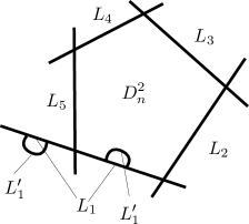
Figure 1. $L^{\prime}_{1}$

We put $L_{i}=L^{\prime}_{i}$ for $i\neq 1$. We may take $L^{\prime}_{1}$ so that (2) holds. (1) is obvious from construction. We observe that there is only one non-trivial operation of positive energy that is

$$\mathfrak{m}_{n-1}:CF(L_{1},L_{2})\otimes\dots\otimes CF(L_{n-1},L_{n})\to CF(L_{1},L_{n})$$

which is induced from the holomorphic $n$-gon $D_{n}^{2}$. It gives

(3.1) $$\mathfrak{m}_{n-1}(p_{1,2},\dots,p_{n-1,n})=T^{\lambda}p_{1,n}$$

where $p_{i,i+1}$ is the generator of $CF(L_{i},L_{i+1})$ corresponding to the intersection point that is a vertex of $D_{n}^{2}$ and $\lambda$ is the area of $D_{n}^{2}$.

If we replace $L_{1}$ by $L^{\prime}_{1}$ we obtain the same conclusion except (3.1) is replaced by

(3.2) $$\mathfrak{m}_{n-1}(p_{1,2},\dots,p_{n-1,n})=T^{\lambda^{\prime}}p_{1,n}$$

where $\lambda^{\prime}<\lambda$. This implies that the Gromov-Hausdorff distance

(3.3) $$d_{\rm GH}(\mathfrak{F}((L_{1},0),\dots,(L_{n},0)),\mathfrak{F}((L^{\prime}_{1},0),\dots,(L^{\prime}_{n},0))$$

is non-zero. Moreover it is easy to see that (3.3) is a continuous function of $\lambda^{\prime}$ (when we take a $\lambda^{\prime}$ parametrized family of $L_{1}^{\prime}$) and it converges to $0$ as $\lambda^{\prime}$ converges to $\lambda$. (It is likely that (3.3) is $\lambda-\lambda^{\prime}$. We do not need to prove it to prove Theorem 3.1.) Thus (4) holds.

We finally prove (3). Let us consider the case of the Figure 1 ($n=5$ in particular) and $i=3$. We take domains $A_{1},B_{1},A_{2},B_{2}$ as in Figure 2.

Figure 2. $A_{1},A_{1},B_{1},B_{2}$

We may take $\Sigma$ so that there are 1-handles $H_{1}$, $H_{2}$ such that $H_{i}$ connects $A_{i}$ to $B_{i}$.

We next take an annulus $S^{1}\times[0,1]$ as follows. It starts at the part of $D^{2}_{n}$ where we modify $L_{1}$ to $L^{\prime}_{1}$. It crosses $L_{3}$ and enters into the domain $A_{1}$. Then it passes through the handle $H_{1}$ to arrive in $B_{1}$. It crosses $L_{1}$ at the part where we modify $L_{1}$ to $L^{\prime}_{1}$ and enters $A_{2}$. It passes through the handle $H_{2}$ to arrive in $B_{2}$. It then comes back. (See Figure 3.)

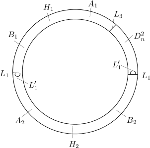
Figure 3. Annulus

The intersection of the annulus $S^{1}\times[0,1]$ with $L_{1}$ is a union of two arcs and it does not intersect with $L_{i}$ other than $L_{1}$ and $L_{3}$.

Now it is easy to see that there exists a symplectic diffeomorphism which has a compact support in the interior of the annulus and which sends $L_{1}$ to $L^{\prime}_{1}$. The proof of Theorem 3.1 is complete. ∎

Remark 3.2.

We remark that in the example we gave above, which is the case of real 2 dimension, the property (4) can be checked very easily and the non-existence of $\varphi:\Sigma\to\Sigma$ suth that $\varphi(L_{i})=L^{\prime}_{i}$ for $i=1,\dots,n$ can be proved by an elementary method. However we can replace $\Sigma$ by $\Sigma\times S^{2}$ and $L_{i},L^{\prime}_{i}$ by $L_{i}\times S^{1}$, $L^{\prime}_{i}\times S^{1}$, respectively, (Here $S^{1}$ is the equator. We take the same equator for $i=1,\dots,n$.) the properties (1)(2)(3)(4) still hold. In this $4$ dimensional case, to prove the non-existence of $\varphi:\Sigma\to\Sigma$ such that $\varphi(L_{i})=L^{\prime}_{i}$ for $i=1,\dots,n$, it seems necessary to use a certain non-elementary method such as pseudo-holomorphic curves, (that is, the Floer theory).

4. Filtered $A_{\infty}$ functors with energy loss.

Let us study the situation where two filtered $A_{\infty}$ categories are close to each other in Gromov-Hausdorff distance. We translate this assumption to another notion, that is, a filtered $A_{\infty}$ functor with energy loss.

Let $\mathscr{C}$ be a filtered $A_{\infty}$ category and $a,b$ its objects. We define:

(4.1) $$\left\{\begin{aligned} &\overset{\circ}{B}_{k}\mathscr{C}[1](a,b):=\underset{a=c_{0},c_{1},\cdots,c_{k-1},c_{k}=b}{\bigoplus}\mathscr{C}[1](c_{0},c_{1})\otimes\cdots\otimes\mathscr{C}[1](c_{k-1},c_{k})\\ &\overset{\circ}{B}\mathscr{C}[1](a,b):=\underset{k=1,2,\dots}{{\bigoplus}}\overset{\circ}{B}_{k}\mathscr{C}[1](a,b).\end{aligned}\right.$$

Let $B\mathscr{C}[1](a,b)$ (resp. $B_{k}\mathscr{C}[1](a,b)$) be the completion of $\overset{\circ}{B}\mathscr{C}[1](a,b)$ (resp. $\overset{\circ}{B}_{k}\mathscr{C}[1](a,b)$) with respect to the energy filtration.

Note that we do not include $k=0$ in (4.1). This is different from the convention of [Fu5, Section 2]. In this paper we assume that a filtered $A_{\infty}$ category satisfies $\mathfrak{m}_{0}=0$.

We define a homomorphism

(4.2) $$\Delta:B_{k}\mathscr{C}[1](a,b)\to\underset{k_{1}+k_{2}=k}{\widehat{\bigoplus}}\underset{c}{\widehat{\bigoplus}}\,\,\,B_{k_{1}}\mathscr{C}[1](a,c)\widehat{\boxtimes}B_{k_{2}}\mathscr{C}[1](c,b)$$

by

(4.3) $$\Delta(x_{1}\otimes\cdots\otimes x_{k})=\sum_{k^{\prime}=1}^{k-1}(x_{1}\otimes\cdots\otimes x_{k^{\prime}})\boxtimes(x_{k^{\prime}+1}\otimes\cdots\otimes x_{k}).$$

This map is co-associative in an obvious sense. Here and hereafter we use $\boxtimes$ in place of $\otimes$ in the right hand sides of (4.2),(4.3). In fact several different kinds of tensor products appear in this paper so it seems necessary to introduce several different notations for tensor products to distinguish them.

The submodule $\overset{\circ}{B}\mathscr{C}[1](a,b)$ is preserved by $\Delta$. We call $\overset{\circ}{B}\mathscr{C}[1](a,b)$ the finite part of $B\mathscr{C}[1](a,b)$

Let $\mathscr{C}$, $\mathscr{C}^{\prime}$ be filtered $A_{\infty}$ categories and $\Phi_{\rm ob}:\mathfrak{OB}(\mathscr{C})\to\mathfrak{OB}(\mathscr{C}^{\prime})$ a set theoretical map. Let $a,b$ be objects of $\mathscr{C}$ and $a^{\prime}=\Phi_{\rm ob}(a)$, $b^{\prime}=\Phi_{\rm ob}(b)$. When a $\Lambda_{0}$ filtered module homomorphism $\Phi_{k}(a,b):B_{k}\mathscr{C}[1](a,b)\to\mathscr{C}^{\prime}[1](a^{\prime},b^{\prime}),$ of degree $0$ is given for each $k,a,b$, there exists uniquely a $\Lambda_{0}$ module homomorphism $\widehat{\Phi}(a,b):B\mathscr{C}[1](a,b)\to B\mathscr{C}^{\prime}[1](a^{\prime},b^{\prime})$ such that:

1. The map $\widehat{\Phi}(a,b)$ is a co-homomorphism. Namely

   (4.4) $$\Delta\circ\widehat{\Phi}(a,b)=\bigoplus_{c}(\widehat{\Phi}(a,c)\boxtimes\widehat{\Phi}(c,b))\circ\Delta.$$

2. The composition of $\widehat{\Phi}(a,b)$ with the projection $B\mathscr{C}[1](a,b)\to\mathscr{C}[1](a,b)$ is $\Phi_{k}(a,b)$ on $B_{k}\mathscr{C}[1](a,b)$.

3. The finite parts are preserved by $\widehat{\Phi}(a,b)$.

Definition 4.1.

A filtered $A_{\infty}$ functor $\Phi$ from $\mathscr{C}$ to $\mathscr{C}^{\prime}$ with energy loss $\rho$ is by definition $(\Phi_{\rm ob},\{\Phi_{k}(a,b)\})$ such that:

1. A set theoretical map $\Phi_{\rm ob}:\mathfrak{OB}(\mathscr{C})\to\mathfrak{OB}(\mathscr{C}^{\prime})$ is given.

2. For objects $a,b$ and $k=1,2,\dots$ $\Phi_{k}(a,b)$ is a $\Lambda$ module homomorphism:

   $$\Phi_{k}(a,b):B_{k}\mathscr{C}_{\Lambda}[1](a,b)\to\mathscr{C}^{\prime}_{\Lambda}[1](a^{\prime},b^{\prime}).$$

   (Note that here we change the coefficient ring from $\Lambda_{0}$ to $\Lambda$.)

3. We obtain $\widehat{\Phi}(a,b):\overset{\circ}{B}\mathscr{C}_{\Lambda}[1](a,b)\to\overset{\circ}{B}\mathscr{C}^{\prime}_{\Lambda}[1](a^{\prime},b^{\prime})$ as above. Then

   $$\widehat{\Phi}(a,b)\circ\hat{d}=\hat{d}\circ\widehat{\mathfrak{F}}(a,b).$$

   Here $\hat{d}$ is the derivation obtained from $A_{\infty}$ operations.

4. We consider the energy filtration $\mathfrak{F}^{\lambda}$ of $B\mathscr{C}_{\Lambda}[1](a,b)$ such that $x_{1}\otimes x_{2}\otimes\dots\otimes x_{k}$ is in $\mathfrak{F}^{\lambda}B\mathscr{C}_{\Lambda}[1](a,b)$ if and only if $x_{i}\in\mathfrak{F}^{\lambda_{i}}(c_{i},c_{i+1})$ with $\sum\lambda_{i}=\lambda$. Then

   $$\Phi_{k}(a,b)(\mathfrak{F}^{\lambda}B_{k}\mathscr{C}_{\Lambda}[1](a,b))\subset\mathfrak{F}^{\lambda-k\rho}\mathscr{C}^{\prime}_{\Lambda}[1](a^{\prime},b^{\prime})$$

Definition 4.2.

We say a filtered $A_{\infty}$ functor $\Phi:\mathscr{C}\to\mathscr{C}^{\prime}$ with energy loss $\rho$ between unital filtered $A_{\infty}$ categories is unital if

$$\Phi_{1}({\bf e}_{a})={\bf e}_{\Phi_{\rm ob}(a)},\quad\Phi_{k}(x_{1},\dots,{\bf e}_{c_{i}},\dots,x_{k})=0,\quad k\geq 2.$$

Here ${\bf e}_{a}\in\mathscr{C}(a,a)$ is the unit.

Note that a filtered $A_{\infty}$ functor $\Phi:\mathscr{C}\to\mathscr{C}^{\prime}$ with energy loss 0 is nothing but a filtered $A_{\infty}$ functor. In [FOOO1, Definition 5.21] we defined the notion of a filtered $A_{\infty}$ bi-module homomorphism with energy loss. Biran-Cornea-Shelukhin [BCS] uses a related notion which they call a weakly filtered $A_{\infty}$ functor with discrepancy.

Lemma 4.3.

Let $\Phi^{n}:\mathscr{C}^{n}\to\mathscr{C}^{n+1}$ be a filtered $A_{\infty}$ functor with energy loss $\rho_{n}$ for $n=1,2$. Then we can compose to obtain $\Phi^{2}\circ\Phi^{1}:\mathscr{C}^{1}\to\mathscr{C}^{3}$ that is a filtered $A_{\infty}$ functor with energy loss $\rho_{1}+\rho_{2}$.

Proof.

We can define a composition as an $A_{\infty}$ functor linear over $\Lambda$. (See for example [Fu2, Definition 7.34].) Then Definition 4.1 (4) can be checked easily from the explicit formula. In fact $\widehat{\Phi^{2}\circ\Phi^{1}}=\widehat{\Phi^{2}}\circ\widehat{\Phi^{1}}$. ∎

Lemma 4.4.

If $\Phi:\mathscr{C}_{1}\to\mathscr{C}_{2}$ is a unital filtered $A_{\infty}$ functor with energy loss $\rho$, then

$$d_{{\rm Hof}}(\Phi_{\rm ob}(c_{1}),\Phi_{\rm ob}(c_{2}))\leq d_{{\rm Hof}}(c_{1},c_{2})+2\rho,$$

Proof.

Let $c_{1},c_{2}\in\mathfrak{OB}(\mathscr{C}_{1})$ and $(t_{12},t_{21},s_{1},s_{2})$ be a homotopy equivalence between them with energy loss $\epsilon$. We put $t^{\prime}_{12}:=\Phi_{1}(t_{12})$, $t^{\prime}_{21}:=\Phi_{2}(t_{21})$ $s^{\prime}_{1}=\Phi_{1}(s_{1})+\Phi_{2}(t_{12},t_{21})$, $s^{\prime}_{2}=\Phi_{1}(s_{2})+\Phi_{2}(t_{21},t_{12})$. It is easy to check that they become a homotopy equivalence between $\Phi_{\rm ob}(c_{1}),\Phi_{\rm ob}(c_{2})$ with energy loss $\epsilon+2\rho$. The lemma follows. ∎

The next corollary is immediate from Lemma 4.4.

Corollary 4.5.

The Hofer distance is invariant under the unital homotopy equivalence of unital filtered $A_{\infty}$ categories.

Definition 4.6.

Let $(C,d)$, $(C^{\prime},d^{\prime})$ be filtered (resp. completed) cochain complexes over $\Lambda_{0}$. A cochain map (resp. completed cochain map) with energy loss $\rho$ from $(C,d)$ to $(C^{\prime},d^{\prime})$ is by definition a cochain map (resp. completed cochain map) $\phi:C_{\Lambda}\to C^{\prime}_{\Lambda}$ such that $\phi(\mathfrak{F}^{\lambda}C_{\Lambda})\subseteq\mathfrak{F}^{\lambda-\rho}C^{\prime}_{\Lambda}$.

Let $\phi,\psi:C_{\Lambda}\to C^{\prime}_{\Lambda}$ be cochain maps with energy loss $\rho$. A cochain homotopy with energy loss $\rho$ between $\phi,\psi$ is $H:C_{\Lambda}\to C^{\prime}_{\Lambda}$ such that $d^{\prime}_{\Lambda}\circ H+H\circ d_{\Lambda}=\phi-\psi^{\prime}$ and $H(\mathfrak{F}^{\lambda}C_{\Lambda})\subseteq\mathfrak{F}^{\lambda-\rho}C^{\prime}_{\Lambda}$. In the case of completed cochain complexes we require that $H$ preserves the finite part.

A cochain map $\phi$ with energy loss $\rho_{1}$ from $(C,d)$ to $(C^{\prime},d^{\prime})$ is said to be a cochain homotopy equivalence with energy loss $\rho$ if there exists a cochain map $\psi$ with energy loss $\rho_{2}$ from $(C^{\prime},d^{\prime})$ to $(C,d)$ with $\rho_{1}+\rho_{2}\leq\rho$ such that the compositions $\phi\circ\psi$ and $\psi\circ\phi$ are cochain homotopy equivalent to the identity map as cochain maps with energy loss $\rho$.

Theorem 4.7.

Suppose $\mathscr{C}_{1}$ and $\mathscr{C}_{2}$ are gapped and unital filtered $A_{\infty}$ categories with $d_{\rm GH}(\mathscr{C}_{1},\mathscr{C}_{2})<\epsilon$. Then there exists a gapped filtered $A_{\infty}$ functor $\Phi:\mathscr{C}_{1}\to\mathscr{C}_{2}$ with energy loss $\epsilon$.

Its linear part $\Phi_{1}:\mathscr{C}_{1}(a,b)\to\mathscr{C}_{2}(\Phi_{\rm ob}(a),\Phi_{\rm ob}(b))$ is a cochain homotopy equivalence with energy loss $2\epsilon$.

The same holds for completed DG-category (which is not necessary gapped).

Proof.

The main part of the proof is the following:

Lemma 4.8.

Let $\mathscr{C}$ be a gapped and unital filtered $A_{\infty}$ category and $\mathfrak{C}_{\mathcal{I}}=\{c_{i}\mid i\in\mathcal{I}\}$, $\mathfrak{C}^{\prime}_{\mathcal{I}}=\{c^{\prime}_{i}\mid i\in\mathcal{I}\}$ are sets of objects. Here $\mathcal{I}$ is a certain index set. We assume that $d_{\rm Hof}(c_{i},c^{\prime}_{i})<\epsilon$ for $i\in\mathcal{I}$. Then there exists a filtered $A_{\infty}$ functor with energy loss $\epsilon$, $\Phi:{\mathscr{C}}(\mathfrak{C}_{\mathcal{I}})\to{\mathscr{C}}(\mathfrak{C}^{\prime}_{\mathcal{I}})$ between full subcategories.

Its linear part is a cochain homotopy equivalence with energy loss $2\epsilon$.

The same holds for completed DG-category (which is not necessary gapped).

Proof.

We may assume that $\mathscr{C}$ is a DG-category. (Here we use gapped-ness.) Note that there is an embedding of filtered $A_{\infty}$ categories $\mathfrak{I}:{\mathscr{C}}(\mathfrak{C}_{\mathcal{K}})\to{\mathscr{C}}(\mathfrak{C}_{\mathcal{K}}\cup\mathfrak{C}^{\prime}_{\mathcal{K}}).$ By [Fu2, Lemma 8.45] $\mathfrak{I}_{\Lambda}:{\mathscr{C}}_{\Lambda}(\mathfrak{C}_{\mathcal{K}})\to{\mathscr{C}}_{\Lambda}(\mathfrak{C}_{\mathcal{K}}\cup\mathfrak{C}^{\prime}_{\mathcal{K}})$ is a homotopy equivalence of $A_{\infty}$ categories over $\Lambda$. Its homotopy inverse $\Psi$ in the case of DG-category is given explicitly in [Fu2, page 115], that is:

(4.5) $$\Psi_{k}(x_{1},\dots,x_{k})=t\circ x_{1}\circ s_{1}\circ x_{2}\circ\dots\circ x_{k-1}\circ s_{k-1}\circ x_{k}\circ t^{\prime}.$$

Here the symbol $\circ$ is obtained from the $\mathfrak{m}_{2}$ operator by putting the sign. Namely

(4.6) $$x\circ y=(-1)^{\deg x}\mathfrak{m}_{2}(x,y),\qquad dx=\mathfrak{m}_{1}(x).$$

Then $\circ$ is associative and $d$ is a coderivation. (See [Fu2, Proof of Lemma 8.45].)

The morphisms $t,t^{\prime},s_{j}$ are defined as follows. Let $x_{j}\in\mathscr{C}(c_{i_{j-1}},c_{i_{j}})$, $j=1,\dots,k$ and $t=t_{c^{\prime}_{i_{0}},c_{i_{0}}}\in\mathscr{C}(c^{\prime}_{i_{0}},c_{i_{0}})$, $t^{\prime}=t_{c_{i_{k}},c^{\prime}_{i_{k}}}\in\mathscr{C}(c_{i_{k}},c^{\prime}_{i_{k}})$ and $s_{j}=s_{c_{i_{j}}}\in\mathscr{C}(c_{i_{j}},c_{i_{j}})$. Here $(t_{c_{i},c^{\prime}_{i}},t_{c^{\prime}_{i},c_{i}},s_{c_{i}},s_{c^{\prime}_{i}})$ is a homotopy equivalence with energy loss $\epsilon$ between $c_{i}$ and $c^{\prime}_{i}$. It is easy to check $\mathfrak{v}(\Psi_{k}(x_{1},\dots,x_{k}))>\sum\mathfrak{v}(x_{j})-k\epsilon,$ that is, $\Psi$ has energy loss $\epsilon$.

The linear part $\Psi_{1}\circ\mathfrak{I}_{1}$ is given by $x\mapsto t\circ x\circ t^{\prime}$. Its cochain homotopy inverse is given by $y\mapsto t^{\prime}\circ x\circ t$. In fact the composition is $x\mapsto t\circ t^{\prime}\circ x\circ t\circ t^{\prime}$ and

$$t^{\prime}\circ t\circ x\circ t\circ t^{\prime}-x=-d(s\circ x\circ t\circ t^{\prime}+x\circ s^{\prime})+(s\circ dx\circ t\circ t^{\prime}+dx\circ s^{\prime}).$$

∎

Now we prove Theorem 4.7. We take $\epsilon^{\prime}$ such that $d_{\rm GH}(\mathscr{C}_{1},\mathscr{C}_{2})<\epsilon^{\prime}<\epsilon.$ We take $\mathscr{C}$ as in Definition 2.5. We take $\mathscr{C}^{0}_{i}$ the full subcategory of $\mathscr{C}_{i}$ with the following properties.

1. The $\epsilon-\epsilon^{\prime}$ neighborhood of $\mathfrak{OB}(\mathscr{C}^{0}_{i})$ contains $\mathfrak{OB}(\mathscr{C}_{i})$.

2. There exists a bijection $I:\mathfrak{OB}(\mathscr{C}^{0}_{i})\to\mathfrak{OB}(\mathscr{C}^{0}_{2})$ such that $d_{\rm Hof}(c,I(c))<\epsilon^{\prime}$ for any $c$.

Applying Lemma 4.8 to $\mathscr{C}^{0}_{1}$ and $\mathscr{C}^{0}_{2}$ we obtain a filtered $A_{\infty}$ functor with energy loss $\epsilon^{\prime}$, $\Phi_{0}$, from $\mathscr{C}^{0}_{1}$ to $\mathscr{C}^{0}_{2}$.

Let $J:\mathfrak{OB}(\mathscr{C}_{1})\to\mathfrak{OB}(\mathscr{C}^{0}_{1})$ be a set theoretical map such that $d_{\rm Hof}(c,J(c))<\epsilon-\epsilon_{1}$. (Note that $J$ may not be continuous.) Using the same formula (4.5) we obtain a filtered $A_{\infty}$ functor $\Phi_{1}:\mathscr{C}_{1}\to\mathscr{C}_{1}^{0}$ of energy loss $\epsilon-\epsilon^{\prime}$ such that it becomes $J$ for objects. The composition of $\Phi_{0}\circ\Phi_{1}$ with the inclusion $\mathscr{C}_{1}^{0}\to\mathscr{C}_{1}$ is the required filtered $A_{\infty}$ functor. ∎

Definition 4.9.

An inductive system of filtered $A_{\infty}$ categories is a pair $((\mathscr{C}^{1},\mathscr{C}^{2},\dots),\linebreak(\Phi^{1},\Phi^{2},\dots))$ such that:

1. A filtered $A_{\infty}$ category $\mathscr{C}^{n}$ is given for $n=1,2,\dots$.

2. A filtered $A_{\infty}$ functor with energy loss $\epsilon_{n}$, $\Phi^{n}:\mathscr{C}^{n}\to\mathscr{C}^{n+1}$ is given for $n=1,2,\dots$.

3. The sum $\sum\epsilon_{n}$ is finite.

Definition 4.10.

An inductive system of filtered $A_{\infty}$ categories is said to be unital (resp. gapped) if filtered $A_{\infty}$ categories and filtered $A_{\infty}$ functors are all unital (resp. gapped). (We remark that the discrete monoid $G$ appearing in the definition of gapped-ness may depend on $n$.)

Theorem 4.11.

Let $(\{\mathscr{C}^{n}\},\{\Phi^{n}\})$ be a gapped inductive system of filtered $A_{\infty}$ categories. Then there exists a completed DG-category ${\mathscr{C}}^{\infty}$ such that:

1. The set of objects of ${\mathscr{C}}^{\infty}$ is identified with the inductive limit as the sets $\varinjlim\mathfrak{OB}({\mathscr{C}}^{n})$. Here we use $\Phi^{n}_{\rm ob}:\mathfrak{OB}({\mathscr{C}}^{n})\to\mathfrak{OB}({\mathscr{C}}^{n+1})$ to define this inductive system.

2. We put $\epsilon^{\prime}_{n}=\sum_{m=n}^{\infty}\epsilon_{m}$. Then there exists a filtered $A_{\infty}$ functor $\Upsilon^{\infty,n}:{\mathcal{C}}^{n}\to{\mathcal{C}}^{\infty}$ with energy loss $\epsilon^{\prime}_{n}$ such that $\Upsilon^{\infty,n+1}\circ\Phi^{n}=\Upsilon^{\infty,n}.$

3. Let $a^{\infty},b^{\infty}\in\mathfrak{OB}({\mathcal{C}}^{\infty})$. We take $a^{m},a^{m+1},\dots$ and $b^{m},b^{m+1},\dots$ which represents $a^{\infty},b^{\infty}$. Then the cohomology group $H({\mathscr{C}}^{\infty}(a^{\infty},b^{\infty}),\mathfrak{m}_{1})$ is almost isomorphic to $H(\varinjlim({\mathscr{C}}^{n}(a^{n},b^{n}),\mathfrak{m}_{1}).$

4. If ${\mathscr{C}}^{n}$, $\Phi^{n}$ are all unital then ${\mathscr{C}}^{\infty}$ is homotopically unital. Moreover $\Upsilon^{\infty,n}$ is homotopically unital.

Theorem 4.11 will be proved in Sections 5-11. We now define the inductive limit appearing in item (3).

Definition 4.12.

An inductive system of filtered cochain complexes over $\Lambda_{0}$ (resp. completed cochain complexes) is $(\{C^{n}\},\{\varphi^{n}\})$ where:

1. A filtered cochain complex $C^{n}$ over $\Lambda_{0}$ (resp. completed cochain complexes $(C^{n},C^{n}_{0})$) is given.

2. A filtered (resp. completed) cochain map $\varphi^{n}:C^{n}\to C^{n+1}$ over $\Lambda_{0}$ with energy loss $\epsilon_{n}$ is given.

3. The sum $\sum\epsilon_{n}$ is finite.

Lemma-Definition 4.13.

We can define the inductive limit of an inductive system of filtered cochain complexes over $\Lambda_{0}$ or completed cochain complexes. The inductive limit is a completed cochain complex in the sense of Definition 2.13.

Proof.

We consider the inductive limit $\varinjlim\,C^{n}_{\Lambda}$ that is a $\Lambda$ vector space, which we denote by $\overset{\circ}{C^{\infty}_{\Lambda}}$. The co-boundary operators $d_{n}$ on $C^{n}_{\Lambda}$ induces a co-boundary operator $d$ on $\overset{\circ}{C^{\infty}_{\Lambda}}$. We define a filtration $\mathfrak{F}^{\lambda}\overset{\circ}{C^{\infty}_{\Lambda}}$ as follows. An element $x^{\infty}$ of $\overset{\circ}{C^{\infty}_{\Lambda}}$ is contained in $\mathfrak{F}^{\lambda}\overset{\circ}{C^{\infty}_{\Lambda}}$ if and only if there exists a sequence $x^{n}\in C^{n}_{\Lambda}$ such that $\lim_{n\to\infty}x^{n}=x^{\infty}$ and that $\mathfrak{v}(x^{n})\geq\lambda_{n}$ with $\lim_{n\to\infty}\lambda_{n}=\lambda$. We put $\overset{\circ}{C^{\infty}}:=\mathfrak{F}^{0}\overset{\circ}{C^{\infty}_{\Lambda}}$. Let $C^{\infty}$ be the completion of $\overset{\circ}{C^{\infty}}$ with respect to the energy filtration. Then $(C^{\infty},\overset{\circ}{C^{\infty}})$ is the completed filtered cochain complex we look for.

In the case of inductive system of compelted cochain complexes we first take the inductive limit of the finite part and then take the completion. ∎

We remark that if $\Phi:\mathscr{C}\to\mathscr{C}^{\prime}$ is a filtered $A_{\infty}$ functor with energy loss $\rho$ then, for objects $a,b$ of $\mathscr{C}$, the map $\Phi_{1}(a,b):\mathscr{C}(a,b)\to\mathscr{C}^{\prime}(\Phi_{\rm ob}(a),\Phi_{\rm ob}(b))$ is a filtered cochain map of energy loss $\rho$. Therefore the inductive limit $\varinjlim({\mathscr{C}}^{n}(a^{n},b^{n}),\mathfrak{m}_{1})$ appearing in Theorem 4.11 (3)(b) is defined in Lemma-Definition 4.13.

Remark 4.14.

Let $(\{C^{n}\},\{\varphi^{n}\})$ be an inductive system of filtered cochain complexes over $\Lambda_{0}$. Suppose in addition that the energy loss of $\varphi^{n}$ is $0$. We obtain the inductive limit in the usual sense. Namely we take the set theoretical inductive limit of $C^{n}$ and define the co-boundary operator as the limit. This inductive limit or its completion, however, may not coincide with one in Lemma-Definition 4.13.

In fact, let us take $C^{n}=\Lambda_{0}$ with $0$ as co-boundary operators. We put $\varphi^{n}(x)=T^{1/2^{n}}x$. The inductive limit in Lemma-Definition 4.13 is $\Lambda_{0}$. The usual inductive limit is $\Lambda_{+}$. We remark that $\Lambda_{+}$ is closed in $\Lambda_{0}$ with respect to the $T$-adic topology.

5. The Bar resolution of a filtered $A_{\infty}$ category.

In this section we describe the Bar-resolution of a filtered $A_{\infty}$ category. The Bar resolution is a well established notion. We give its definition here since we need to study various filtrations carefully.

Definition 5.1.

A doubly filtered differential graded co-category $\mathscr{B}$ is the following object. Hereafter we write DFDGC instead of doubly filtered differential graded co-category.

1. The set of objects, $\mathfrak{OB}(\mathscr{B})$, is given.

2. For each $a,b\in\mathfrak{OB}(\mathscr{B})$ a completed cochain complex over $\Lambda_{0}$, abbreviated by $\mathscr{B}(a,b)$, is given. Its filtration $\mathfrak{F}^{\mathfrak{\lambda}}\mathscr{B}(a,b)$ is called the energy filtration. We denote the finite part of $\mathscr{B}(a,b)$ by $\overset{\circ}{\mathscr{B}}(a,b)$

3. Another filtration $\mathfrak{S}^{k}\mathscr{B}(a,b)$, abbreviated by number filtration, is given such that:

   1. For $k=1,2,\dots$ $\mathfrak{S}^{k}\mathscr{B}(a,b)$ is a completed subcomplex of $\mathscr{B}(a,b)$ with $\mathfrak{S}^{k}\overset{\circ}{\mathscr{B}}(a,b)$ being its finite part.

   2. $\mathfrak{S}^{k+1}\mathscr{B}(a,b)\supseteq\mathfrak{S}^{k}\mathscr{B}(a,b)$.

   3. We require $\overset{\circ}{\mathscr{B}}(a,b):=\bigcup_{n}\mathfrak{S}^{n}\overset{\circ}{\mathscr{B}}(a,b).$

4. A map $\Delta:\overset{\circ}{\mathscr{B}}(a,b)\to\underset{c}{{\bigoplus}}\overset{\circ}{\mathscr{B}}(a,c)\boxtimes\overset{\circ}{\mathscr{B}}(c,b).$ is given. We call it the co-composition. It induces $\Delta:{\mathscr{B}}(a,b)\to\underset{c}{\widehat{\bigoplus}}{\mathscr{B}}(a,c)\widehat{\boxtimes}{\mathscr{B}}(c,b).$

5. The co-composition is co-associative and preserves co-derivation and two filtrations.

Definition 5.2.

To a filtered $A_{\infty}$ category $\mathscr{C}$ we associate a DFDGC $B\mathscr{C}$ as follows. We call $B\mathscr{C}$ the Bar resolution of $\mathscr{C}$.

1. The set of objects is defined by $\mathfrak{OB}(B\mathscr{C}):=\mathfrak{OB}(\mathscr{C})$.

2. The finite part of the morphism space $\overset{\circ}{B}\mathscr{C}(a,b)$ is defined by (4.1). $B\mathscr{C}(a,b)$ is its completion. The co-boundary operator is the co-derivation $\hat{d}$ induced from the $A_{\infty}$ operations $\mathfrak{m}_{k}$. The energy filtration of $B\mathscr{C}(a,b)$ is induced from the energy filtration of $\mathscr{C}(a,b)$ in an obvious way.

3. The number filtration is defined by: $\mathfrak{S}^{k}\overset{\circ}{B}\mathscr{C}(a,b):=\bigoplus_{\ell=1}^{k}\overset{\circ}{B}_{\ell}\mathscr{C}(a,b).$ Here the right hand side is defined by (4.1).

4. The co-composition is defined by (4.3). It is obvious that it is co-associative and preserves two filtrations. Moreover $\hat{d}$ is a co-derivation and preserves two filtrations.

Definition 5.3.

Let $\mathscr{B}$, $\mathscr{B}^{\prime}$ be DFDGCs. A DFDGC morphism with energy loss $\rho$ from $\mathscr{B}$ to $\mathscr{B}^{\prime}$ is $\Psi:=(\Psi_{\rm ob},\Psi_{\Lambda})$ where:

1. A map $\Psi_{\rm ob}:\mathfrak{OB}(\mathscr{B})\to\mathfrak{OB}(\mathscr{B}^{\prime})$ is given.

2. Let $a^{\prime}=\Psi_{\rm ob}(a)$, $b^{\prime}=\Psi_{\rm ob}(b)$. Then a $\Lambda$ linear map $\Psi_{\Lambda}(a,b):\overset{\circ}{\mathscr{B}}_{\Lambda}(a,b)\to\overset{\circ}{\mathscr{B}^{\prime}}_{\Lambda}(a^{\prime},b^{\prime})$ of degree $0$ is given. The map $\Psi_{\Lambda}(a,b)$ preserves the number filtration and the finite part.

3. The linear map $\Psi_{\Lambda}$ is a co-homomorphism. Namely $\Delta\circ{\Psi_{\Lambda}}(a,b)=\bigoplus_{c}({\Psi_{\Lambda}}(a,c)\boxtimes{\Psi_{\Lambda}}(c,b))\circ\Delta.$ on $\overset{\circ}{\mathscr{B}}_{\Lambda}(a,b)$.

4. We require

   (5.1) $$\Psi_{\Lambda}(a,b)(\mathfrak{F}^{\lambda}\mathfrak{S}^{k}(\overset{\circ}{\mathscr{B}}(a,b)))\subseteq\mathfrak{F}^{\lambda-k\rho}\mathfrak{S}^{k}(\overset{\circ}{\mathscr{B}^{\prime}}(a^{\prime},b^{\prime})).$$

   In particular $\Psi_{\Lambda}(a,b)$ induces a map: $\mathfrak{F}^{\lambda}\mathfrak{S}^{k}({\mathscr{B}}(a,b))\to\mathfrak{F}^{\lambda-k\rho}\mathfrak{S}^{k}({\mathscr{B}^{\prime}}(a^{\prime},b^{\prime}))$.

Definition 5.4.

Let $\Phi:\mathscr{C}\to\mathscr{C}^{\prime}$ be a filtered $A_{\infty}$ functor with energy loss $\rho$. It induces a DFDGC morphism with with energy loss $\rho$, which is abbreviated by $B\Phi:B\mathscr{C}\to B\mathscr{C}^{\prime}$, as follows.

1. The map $(B\Phi)_{\rm ob}:\mathfrak{OB}(B\mathscr{C})\to\mathfrak{OB}(B\mathscr{C}^{\prime})$ is $\Phi_{\rm ob}$.

2. Let $a^{\prime}=\Phi_{\rm ob}(a)$, $b^{\prime}=\Phi_{\rm ob}(b)$. The map $(B\Phi)_{\Lambda}(a,b):\overset{\circ}{\mathscr{B}}_{\Lambda}(a,b)\to\overset{\circ}{\mathscr{B}^{\prime}}_{\Lambda}(a^{\prime},b^{\prime})$ is obtained in Definition 4.1 (3).

The fact that they satisfy (1)-(4) of Definition 5.3 is immediate from Definition 4.1.

Definition 5.5.

An inductive system of DFDGC is $(\{\mathscr{B}^{n}\},\{\Psi^{n}\})$ where:

1. A DFDGC $\mathscr{B}^{n}$ is given for $n=1,2,\dots$.

2. A DFDGC morphism with energy loss $\epsilon_{n}$, $\Psi^{n}:\mathscr{B}^{n}\to\mathscr{B}^{n+1}$, is given for $n=1,2,\dots$.

3. The sum $\sum\epsilon_{n}$ is finite.

Lemma 5.6.

If $(\{\mathscr{C}^{n}\},\{\Phi^{n}\})$ is an inductive system of filtered $A_{\infty}$ categories, then $(\{B\mathscr{C}^{n}\},\{B\Phi^{n}\})$ is an inductive system of DFDGC.

The proof is obvious. Note that the maps appearing in the morphisms of DFDGC are linear, while the maps appearing in the filtered $A_{\infty}$ functors are multi-linear (or non-linear). By this reason taking the inductive limit is much easier for DFDGC than for filtered $A_{\infty}$ categories.

Definition 5.7.

Let $(\{\mathscr{B}^{n}\},\{\Psi^{n}\})$ be an inductive system of DFDGC. We define its inductive limit, abbreviated by $\varinjlim\,{\mathscr{B}}^{n}$, as follows. We put ${\mathscr{B}}^{\infty}=\,\varinjlim{\mathscr{B}}^{n}$.

1. The set $\mathfrak{OB}({\mathscr{B}}^{\infty})$ of its objects is the inductive limit $\varinjlim\,\mathfrak{OB}({\mathscr{B}}^{n})$ as sets. Note that we use $\Psi^{n}_{\rm ob}$ to define this inductive system.

2. Let $a^{\infty},b^{\infty}$ be elements of ${\mathscr{B}}^{\infty}$. We take sequences $a^{n}$, $b^{n}$ of elements $\mathfrak{OB}({\mathscr{B}}^{n})$ representing $a^{\infty},b^{\infty}$, respectively. We put

   (5.2) $$\mathfrak{S}^{k}{\mathscr{B}}^{\infty}(a^{\infty},b^{\infty})=\varinjlim\,\mathfrak{S}^{k}{\mathscr{B}}^{n}(a^{n},b^{n}).$$

   Note that $\mathfrak{S}^{k}{\mathscr{B}}^{n}(a^{n},b^{n})$ together with $\Psi^{n}_{\Lambda}(a^{n},b^{n})$ becomes an inductive system of completed cochain complexes. Therefore the inductive limit in the right hand side of (5.2) is defined by Lemma-Definition 4.13.

3. We put $\overset{\circ}{\mathscr{B}^{\infty}}(a,b):=\bigcup_{n}\mathfrak{S}^{n}\overset{\circ}{\mathscr{B}^{\infty}}(a,b)$ and define ${\mathscr{B}}^{\infty}(a,b)$ to be its completion with respect to the energy filtration.

4. Since $\Psi^{n}$ preserves co-composition $\Delta$ it induces a co-composition $\Delta$ on the inductive limit.

It is easy to see that the axiom of DFDGC is satisfied.

6. Back to $A_{\infty}$ category via Co-Bar resolution.

Let $(\{\mathscr{C}^{n}\},\{\Phi^{n}\})$ be an inductive system of filtered $A_{\infty}$ categories. By Lemma 5.6 and Definition 5.7 we obtain a DFDGC $\mathscr{B}^{\infty}$ by

(6.1) $$\mathscr{B}^{\infty}:=\varinjlim\,B{\mathscr{C}}^{n}.$$

Note that by Lemma-Definition 4.13 we have an inductive limit

(6.2) $$\mathscr{C}^{\infty}(a,b):=\varinjlim\,{\mathscr{C}}^{n}(a^{n},b^{n}),$$

which is a completed cochain complex if $a=\lim a_{n}$ and $b=\lim b_{n}$. In particular the boundary operator $\mathfrak{m}_{1}$ is induced on it. However its $A_{\infty}$ operations $\mathfrak{m}_{k}$ for $k>1$ is not given.

We define a few maps between $B{\mathscr{C}}^{n}(a_{n},b_{n})$, $\mathscr{B}^{\infty}(a,b)$. Let $a_{n},b_{n}\in\mathfrak{OB}(\mathscr{C}^{n})$. For $n^{\prime}>n$ we define $a_{n^{\prime}},b_{n^{\prime}}$ inductively by $a_{n^{\prime}+1}=\Phi^{n^{\prime}+1,n^{\prime}}_{\rm ob}(a_{n^{\prime}})$, $b_{n^{\prime}+1}=\Phi^{n^{\prime}+1,n^{\prime}}_{\rm ob}(b_{n^{\prime}})$. We then define $\hat{\Phi}^{n^{\prime},n}(a_{n},b_{n}):\overset{\circ}{B}\mathscr{C}^{n}(a_{n},b_{n})\to\overset{\circ}{B}\mathscr{C}^{n^{\prime}}(a_{n^{\prime}},b_{n^{\prime}})$ by

(6.3) $$\hat{\Phi}^{n^{\prime},n}(a_{n},b_{n}):=\hat{\Phi}^{n^{\prime},n^{\prime}-1}(a_{n^{\prime}-1},b_{n^{\prime}-1})\circ\dots\circ\hat{\Phi}^{n+1,n}(a_{n},b_{n})$$

We put $a_{\infty}=\lim a_{n}$ $b_{\infty}=\lim b_{n}$. We define

(6.4) $$\hat{\Phi}^{\infty,n}(a_{n},b_{n}):\overset{\circ}{B}\mathscr{C}^{n}(a_{n},b_{n})\to\overset{\circ}{\mathscr{B}^{\infty}}(a_{\infty},b_{\infty})$$

by sending ${\bf x}$ to an element represented by $(\hat{\Phi}^{n^{\prime},n}({\bf x}))_{n^{\prime}=n}^{\infty}$. We have the following:

(6.5) $$\hat{\Phi}^{\infty,n}(a_{n},b_{n})(\mathfrak{F}^{\lambda}\mathfrak{S}^{k}\overset{\circ}{B}\mathscr{C}^{n}(a_{n},b_{n}))\subseteq\mathfrak{F}^{\lambda-k\epsilon_{n}}\mathfrak{S}^{k}\overset{\circ}{\mathscr{B}^{\infty}}(a_{\infty},b_{\infty})$$

with $\epsilon_{n}\to 0$.

We use the Co-Bar resolution to define the inductive limit of filtered $A_{\infty}$ categories. The notion of a Co-Bar resolution is classical. (See for example [Ke].) We however give a detailed proof since again we need to study its relation to the two filtrations. We also need to use operations and notations we introduce below in later sections. Let $\mathscr{B}$ be a DFDGC. For its objects $a,b$, we consider

(6.6) $$\left\{\begin{aligned} \overset{\circ}{A}_{k}\mathscr{B}[1](a,b)&=\underset{a=c_{0},c_{1},\cdots,c_{k-1},c_{k}=b}{{\bigoplus}}\overset{\circ}{\mathscr{B}}[1](c_{0},c_{1})\boxtimes\cdots\boxtimes\overset{\circ}{\mathscr{B}}[1](c_{k-1},c_{k})\\ \overset{\circ}{A}\mathscr{B}[1](a,b)&=\underset{k=1,2,\dots}{{\bigoplus}}\overset{\circ}{A}_{k}\mathscr{B}[1](a,b).\end{aligned}\right.$$

The energy filtration of $\mathscr{B}[1](a,b)$ induces an energy filtration of $\overset{\circ}{A}\mathscr{B}[1](a,b)$. Here we use $A$ and $\boxtimes$ in place of $B$ and $\otimes$ to distinguish Co-Bar resolution from Bar resolution. (The symbol $A$ stands for Adams, who introduced Co-Bar resolution in [Ad]. The symbol $F$ is used in some of the references. I avoid it since $F$ is used for filtration.) Let $A_{k}\mathscr{B}[1](a,b)$ be the completion of $\overset{\circ}{A}_{k}\mathscr{B}[1](a,b)$ with respect to the energy filtration. The co-boundary operator $d$ and co-composition $\Delta$ induces operations

(6.7) $$\left\{\begin{aligned} \partial:A\mathscr{B}[-1](a,b)\to A\mathscr{B}[-1](a,b)\\ \hat{\Delta}:A\mathscr{B}[-1](a,b)\to A\mathscr{B}[-1](a,b)\end{aligned}\right.$$

by

(6.8) $$\left\{\begin{aligned} \partial(x_{1}\boxtimes\dots\boxtimes x_{k})&=\sum_{i=1}^{k}(-1)^{*}x_{1}\boxtimes\dots\boxtimes d(x_{i})\boxtimes\dots\boxtimes x_{k},\\ \hat{\Delta}(x_{1}\boxtimes\dots\boxtimes x_{k})&=\sum_{i=1}^{k}(-1)^{*}x_{1}\boxtimes\dots\boxtimes\Delta(x_{i})\boxtimes\dots\boxtimes x_{k},\end{aligned}\right.$$

where $*=\deg^{\prime}x_{1}+\dots+\deg^{\prime}x_{i-1}$. Note that the co-derivation $\Delta$ appearing in the right hand side is a map $\Delta:\mathscr{B}[-1](a,b)\to\widehat{\bigoplus_{c}}\,\,\,\mathscr{B}[-1](a,c)\,\,\widehat{\boxtimes}\,\,\mathscr{B}[-1](c,b).$ It satisfies $\Delta(\overset{\circ}{\mathscr{B}}[-1](a,b))\subseteq{\bigoplus_{c}}\,\,\,\overset{\circ}{\mathscr{B}}[-1](a,c)\,\,{\boxtimes}\,\,\overset{\circ}{\mathscr{B}}[-1](c,b).$ We put

(6.9) $$\mathfrak{M}_{1}:=\partial+\hat{\Delta}:(A\mathscr{B}[-1](a,b))[1]\to(A\mathscr{B}[-1](a,b))[1].$$

We also define:

(6.10) $$\mathfrak{M}_{2}:(A\mathscr{B}[-1](a,c))[1]\,\oslash(A\mathscr{B}[-1](c,b))[1]\to(A\mathscr{B}[-1](a,b))[1]$$

by

(6.11) $$\mathfrak{M}_{2}(x_{1}\boxtimes\dots\boxtimes x_{k}\oslash x_{k+1}\boxtimes\dots\boxtimes x_{m})=(-1)^{*}x_{1}\boxtimes\dots\boxtimes x_{k}\boxtimes x_{k+1}\boxtimes\dots\boxtimes x_{m}$$

with $*=\deg^{\prime}x_{1}+\dots+\deg^{\prime}x_{i-1}+1$. Here $\oslash$ is a tensor product. We use this symbol to distinguish it from $\otimes$, $\boxtimes$. The operators $\mathfrak{M}_{1}$ and $\mathfrak{M}_{2}$ has degree $1$. It is easy to see

(6.12) $$\left\{\begin{aligned} &\mathfrak{M}_{1}\circ\mathfrak{M}_{1}=0,\\ &\mathfrak{M}_{1}(\mathfrak{M}_{2}({\bf x}\oslash{\bf y}))+\mathfrak{M}_{2}(\mathfrak{M}_{1}({\bf x})\oslash{\bf y}))+(-1)^{\deg^{\prime}{\bf x}}\mathfrak{M}_{2}({\bf x}\oslash\mathfrak{M}_{1}({\bf y})))=0.\end{aligned}\right.$$

Moreover $\mathfrak{M}_{1}$ and $\mathfrak{M}_{2}$ preserve the energy filtration. Therefore putting $\mathfrak{M}_{k}=0$ for $k=3,4,\dots$ we obtain a filtered $A_{\infty}$ category. We denote it by $A\mathscr{B}$ also. Since $\mathfrak{M}_{k}=0$ for $k=3,4,\dots$, $A\mathscr{B}$ is actually a DG-category. However the sign convention is one of an $A_{\infty}$ category. (In other words we need a sign change to obtain a DG-category.)

We define the total number filtration $\mathfrak{S}^{n}\overset{\circ}{A}\mathscr{B}$ so that $\mathfrak{S}^{n}\overset{\circ}{A\mathscr{B}}$ is the sub-$\Lambda_{0}$-module generated by the union of

$$\mathfrak{S}^{n_{1}}\overset{\circ}{\mathscr{B}}[1](c_{0},c_{1})\boxtimes\cdots\boxtimes\mathfrak{S}^{n_{k}}\overset{\circ}{\mathscr{B}}[1](c_{k-1},c_{k})$$

with $n_{1}+\dots+n_{k}\leq n$. We remark that $A\mathscr{B}$ is the completion of $\overset{\circ}{A}\mathscr{B}:=\bigcup_{n}\mathfrak{S}^{n}\overset{\circ}{A}\mathscr{B}$.

$A\mathscr{B}$ becomes a completed DG-category. Its finite part is $\overset{\circ}{A}\mathscr{B}$.

Definition 6.1.

We call the completed DG-category $A\mathscr{B}$ the Co-Bar resolution of $\mathscr{B}$.

Let $(\{\mathscr{C}^{n}\},\{\Phi^{n}\})$ be an inductive system of filtered $A_{\infty}$ categories. We put $\mathscr{B}^{\infty}:=\varinjlim\,B{\mathscr{C}}^{n}.$ Then $A\mathscr{B}^{\infty}$ is a completed DG-category.

Definition 6.2.

We define

$$\varinjlim\,{\mathscr{C}}^{n}:=A\mathscr{B}^{\infty}$$

to be the inductive limit of an inductive system of filtered $A_{\infty}$ categories.

We remark that $\varinjlim\,{\mathscr{C}}^{n}(a,b)=\mathfrak{S}^{1}\mathscr{B}^{\infty}(a,b)=\mathfrak{S}^{1}A\mathscr{B}^{\infty}(a,b).$ Here the inductive limit in the left hand side is one as filtered cochain complexes over $\Lambda_{0}$. Therefore there exists a completed injection

(6.13) $$I:({\mathscr{C}}^{\infty}(a,b),\mathfrak{m}_{1})\to(A\mathscr{B}^{\infty}(a,b),\mathfrak{M}_{1}).$$

Theorem 6.3.

The completed injection $I$ is an almost cochain homotopy equivalence.

Corollary 6.4.

The map $I_{*}:H({\mathscr{C}}^{\infty}(a,b),\mathfrak{m}_{1})\to H(A\mathscr{B}^{\infty}(a,b),\mathfrak{M}_{1})$ is an almost isomorphism of $\Lambda_{0}$ modules.

This is a consequence of Theorem 6.3 and Lemma 2.15. We prove Theorem 6.3 in the next section.

7. Almost cochain homotopy equivalence: the proof of Theorem 6.3.

We begin with the following, which seems to be known to experts at least in the case of DG or $A_{\infty}$ category over a filed, such as $\Lambda$ or $R$. We remark that if $\mathscr{C}$ is gapped then $AB\mathscr{C}$ is gapped.

Theorem 7.1.

Let $\mathscr{C}$ be a gapped filtered $A_{\infty}$ category. Then there exists a gapped homotopy equivalence of filtered $A_{\infty}$ categories

$$\mathfrak{I}=(I_{1},I_{2},.\dots):\mathscr{C}\to AB\mathscr{C}$$

so that the linear part $I_{1}$ is the inclusion $I:\mathscr{C}=\mathfrak{S}^{1}AB\mathscr{C}\subseteq A_{1}B\mathscr{C}$.

Proof.

We write an element of $AB\mathscr{C}$ as

(7.1) $${\bf x}=x_{1}\odot_{1}x_{2}\odot_{2}\dots\odot_{m-1}x_{m-1}\odot x_{m}$$

where $\odot_{i}$ is one of $\boxtimes$ or $\otimes$ and $x_{i}\in\mathscr{C}(c,c^{\prime})$ for certain elements $c,c^{\prime}\in\mathfrak{OB}(\mathscr{C})$. We define $\deg\otimes=0$, $\deg\boxtimes=1$.

The co-boundary operator $\mathfrak{M}_{1}$ is the sum of the operations of the forms (I), (II) below.

1. Replacing $\otimes$ to $\boxtimes$. Namely

   (7.2) $$x_{1}\odot_{1}\dots\odot_{k-1}x_{k}\otimes x_{k+1}\odot_{k+2}\dots\odot_{k}x_{m}$$

   $$\mapsto(-1)^{*}x_{1}\odot_{1}\dots\odot_{k-1}x_{k}\boxtimes x_{k+1}\circ_{k+2}\dots\odot_{k}x_{m}$$

   where $*=\deg^{\prime}x_{1}+\deg\odot_{1}+\dots+\deg^{\prime}x_{k-1}+\deg\odot_{k-1}$. The sum of such operations is $\hat{\Delta}$.

2. Applying $\mathfrak{m}_{k}$ to $x_{i+1}\otimes\dots\otimes x_{i+k}$. In other words

   (7.3) $$x_{1}\odot_{1}\dots\odot_{i-1}x_{i}\odot_{i}x_{i+1}\otimes\dots\otimes x_{i+k}\odot_{i+k+1}\dots\odot_{m}x_{m}$$

   $$\mapsto(-1)^{*}x_{1}\odot_{1}\dots\odot_{i}\mathfrak{m}_{k}(x_{i+1},\dots,x_{i+k})\odot_{i+k+1}\dots\odot_{m}x_{m}$$

   Here we require $\odot_{i+1}=\dots=\odot_{i+k}=\otimes$. The sign is $*=\deg^{\prime}x_{1}+\deg\odot_{1}+\dots+\deg^{\prime}x_{k-1}+\deg\odot_{i}$.

For a given $k$ we denote the sum of such operations by $\partial_{k}$. The sum $\widehat{\Delta}+\sum_{k=1}^{\infty}\partial_{k}$ is the co-boundary operator of $AB\mathscr{C}$.

Definition 7.2.

We define the operator $S$ as the sum of the following operations

(7.4) $$x_{1}\odot_{1}\dots\odot_{k-1}x_{k}\boxtimes x_{k+1}\odot_{k+2}\dots\odot_{m}x_{m}$$

$$\mapsto(-1)^{*}x_{1}\odot_{1}\dots\odot_{k-1}x_{k}\otimes x_{k+1}\odot_{k+2}\dots\odot_{m}x_{m}.$$

Namely we replace one of $\boxtimes$ to $\otimes$. The sign is $*=\deg^{\prime}x_{1}+\deg\odot_{1}+\dots+\deg\odot_{i}$.

One can easily check the next formula:

(7.5) $$\left\{\begin{aligned} &(\hat{\Delta}\circ S+S\circ\hat{\Delta})({\bf x})=m-1,\\ &\partial_{1}\circ S+S\circ\partial_{1}=0.\end{aligned}\right.$$

Here $m$ is as in (7.1). Moreover we have

(7.6) $$\partial_{k}(\mathfrak{S}^{m}AB\mathscr{C})\subseteq\mathfrak{S}^{m-1}AB\mathscr{C}$$

for $k\geq 2$. Therefore

(7.7) $$H\left(\frac{\mathfrak{S}^{m}AB\mathscr{C}}{\mathfrak{S}^{m-1}AB\mathscr{C}},\mathfrak{M}_{1}\right)=0$$

for $m>1$. (We use the fact that the ground ring is a field of characteristic $0$ here.) It implies that $I=I_{1}$ induces an isomorphism on cohomologies.

More precisely (7.7) implies that the cohomology of $\overset{\circ}{A}B\mathscr{C}(a,b)$ with $\mathfrak{M}_{1}$ as coboundary operator is isomorphic to the cohomology of $\mathscr{C}(a,b)$ with $\mathfrak{m}_{1}$ as coboundary operator. We need to show that the inclusion induces an isomorphism between the cohomology of $\overset{\circ}{A}B\mathscr{C}(a,b)$ and the cohomology of its completion $AB\mathscr{C}(a,b)$. The proof of this fact is similar to the proof of Lemma 2.15 or of Theorem 6.3. So we omit it.

To complete the proof it suffices to find $I_{k}$ for $k=2,\dots$ such that $\mathfrak{I}=(I_{1},I_{2},\dots)$ becomes an $A_{\infty}$ functor. We define: $I_{k}:\mathscr{C}[1](c_{0},c_{1})\widehat{\oslash}\cdots\widehat{\oslash}\mathscr{C}[1](c_{k-1},c_{k})\to AB\mathscr{C}(c_{0},c_{k})$ by

(7.8) $$I_{k}(x_{1}\oslash\cdots\oslash x_{k}):=x_{1}\otimes\cdots\otimes x_{k}.$$

Namely we replace all the $\oslash$ to $\otimes$. Note that the right hand side is an element of $B_{k}\mathscr{C}[1](c_{0},c_{k})=B\mathscr{C}(c_{0},c_{1})\subseteq A_{1}B\mathscr{C}(c_{0},c_{1})$. It is straitforward to check that (7.8) defines an $A_{\infty}$ functor. ∎

Remark 7.3.

The fact that the composition of the Bar and the Co-Bar resolutions is equivalent to the identity functor is well established. (See for example [Ke].) Since the author could not find the simple formula (7.8) in the literature, he includes it here. Note that even in the case when $\mathscr{C}$ is a DG-category the map $I_{2}$ is non-zero. Namely $\mathfrak{I}$ is not a DG functor. So in the literature the process of inverting the weak equivalence is used. By using the language of $A_{\infty}$ category we can explicitly construct a homotopy equivalence.

Proof of Theorem 6.3.

We begin with the following definition.

Definition 7.4.

Let $(C_{i},C_{i,0})$ be a completed cochain complex for $i=0,1,2$ and $\mathfrak{i}_{i}:(C_{i},C_{i,0})\to(C_{i+1},C_{i+1,0})$ a completed injection for $i=0,1$. We say $\mathfrak{i}_{1}$ is almost cochain homotopy equivalance relative to $C_{0}$ if the following holds. For any finitely generated subcomplex $W$ of $C_{2,0}$ and $\epsilon>0$ there exists $G:W\to C_{2,0}$ such that

1. The image of $dG+Gd-T^{\epsilon}$ is in $C_{1,0}$.

2. $G=0$ on $C_{0,0}$.

3. $G$ preserves energy filtration.

We call $G$ a $\epsilon$-$W$ shrinker relative to $C_{0}$.

Lemma 7.5.

Let $(C_{i},C_{i,0})$ be a completed cochain complex for $i=1,2,3$ , and $\mathfrak{i}_{i}:(C_{i},C_{i,0})\to(C_{i+1},C_{i+1,0})$ a completed injection for $i=0,1,2$. Suppose $\mathfrak{i}_{1}$ and $\mathfrak{i}_{2}$ are almost cochain homotopy equivalences relative to $C_{0}$. Then the composition $\mathfrak{i}_{2}\circ\mathfrak{i}_{1}:(C_{1},C_{1,0})\to(C_{3},C_{3,0})$ is an almost cochain homotopy equivalence relative to $C_{0}$.

Proof.

Let $W\subset C_{3,0}$ and $\epsilon>0$. We take $\epsilon-W$ shrinker $G_{1}$ relative to $C_{0}$ (for $\mathfrak{i}_{2}$). We take $W^{+}$ which contains $W$, $G_{1}W$. We then take $\epsilon-{W^{+}}$-shrinker $G_{2}$ relative to $C_{0}$ (for $\mathfrak{i}_{1}$). We observe

$$(T^{\epsilon}-(dG_{2}+G_{2}d))\circ(T^{\epsilon}-(dG_{1}+G_{1}d))(W)\subset C_{1}.$$

Since $(T^{\epsilon}-(dG_{2}+G_{2}d))\circ(T^{\epsilon}-(dG_{1}+G_{1}d))=T^{2\epsilon}-T^{\epsilon}(d(G_{1}+G_{2})+(G_{1}+G_{2})d)+(dG_{2}G_{1}+G_{2}G_{1}d)$, the map $G:=T^{\epsilon}(G_{1}+G_{2})-G_{2}G_{1}$ is a $2\epsilon-W$ shrinker relative to $C_{0}$ we look for. ∎

Lemma 7.6.

Let $(C_{i},C_{i,0})$ $i=1,2,\dots$ and $(C,C_{0})$ be completed cochain complexes, and the cochain homomorphisms $(C_{i},C_{i,0})\to(C_{i+1},C_{i+1,0})$ completed injections. We assume $C_{0}=\bigcup_{i}C_{i,0}.$ We also assume that $(C_{i},C_{i,0})\to(C_{i+1},C_{i+1,0})$ is an almost cochain homotopy equivalence for $i=1,2,\dots$.

Then $(C_{1},C_{1,0})\to(C,C_{0})$ is an almost cochain homotopy equivalence.

Proof.

By Lemma 7.5 the inclusion $C_{1}\to C_{k}$ is an almost cochain homotopy equivalence. Since any finitely generated subcomplex of $C_{0}$ is contained in $C_{k,0}$ for some $k$, the lemma follows. ∎

Therefore to prove Theorem 6.3 it suffices to show the next lemma.

Lemma 7.7.

The inclusion $\mathfrak{S}^{m-1}A\mathscr{B}^{\infty}[-1](a,b)\to\mathfrak{S}^{m}A\mathscr{B}^{\infty}[-1](a,b)$ is an almost cochain homotopy equivalence relative to ${\mathscr{C}}^{\infty}(a,b)=\mathfrak{S}^{1}A\mathscr{B}^{\infty}[-1](a,b)$.

Proof.

We begin with the following sublemma.

Sublemma 7.8.

Let $W$ be a finitely generated subcomplex of $\mathfrak{S}^{m}\overset{\circ}{A}\mathscr{B}^{\infty}(a,b).$ Then for any sufficiently large $n$ there exists $W^{n}\subset\mathfrak{S}^{m}\overset{\circ}{A}B\mathscr{C}^{n}(a,b)_{\Lambda}$ such that

1. $W^{n}$ is a subcomplex.

2. The restriction of $A\widehat{\Phi}^{\infty,n}$ defines an isomorphism $W^{n}\to W$.

3. For $w\in W^{n}$ we have

   (7.9) $$|\mathfrak{v}(w)-\mathfrak{v}(A\widehat{\Phi}^{\infty,n}(w))|\leq\epsilon_{n}$$

   with $\lim_{m\to\infty}\epsilon_{n}=0$.

4. $$A\widehat{\Phi}^{\infty,n}\left(\mathfrak{S}^{0}\overset{\circ}{A}B\mathscr{C}^{n}[-1](a,b)\cap W_{n}\right)=\mathfrak{S}^{0}\overset{\circ}{A}\mathscr{B}^{\infty}[-1](a,b)\cap W.$$

Proof.

Let $y_{1},\dots,y_{k}$ be a basis of $W_{\Lambda}$ such that $\mathfrak{v}(y_{i})=0$. (Since $W$ is zero energy generated there exists such a basis.) Then taking $n_{0}$ large there exists $\hat{y}_{i}\in\mathfrak{S}^{m}\overset{\circ}{A}B\mathscr{C}^{n_{0}}(a,b)_{\Lambda}$ such that $A\widehat{\Phi}^{\infty,n_{0}}(\hat{y}_{i})=y_{i}$ and $|\mathfrak{v}(\hat{y}_{i})-\mathfrak{v}(y_{i})|\leq\epsilon_{n_{0}}.$ Since $W$ is a subcomplex there exists $a_{i,j}\in\Lambda_{0}$ such that $\mathfrak{M}_{1}(y_{i})=\sum_{j}a_{i,j}y_{j}.$ Therefore for sufficiently large $n$, $y^{\prime}_{i}:=A\widehat{\Phi}^{n,n_{0}}(\hat{y}_{i})$ satisfies the equation $\mathfrak{M}_{1}(y^{\prime}_{i})=\sum_{j}a_{i,j}y^{\prime}_{j}.$ The subcomplex $W^{n}=\mathfrak{F}^{0}(\sum\Lambda y^{\prime}_{i})$ has the properties (1)(2)(3). Since total number filtration is preserved by $A\widehat{\Phi}^{\infty,n_{0}}$ we may choose $\hat{y}_{i}$ so that (4) is satisfied. ∎

Now we prove Lemma 7.7. Let $W$ be a finitely generated subcomplex of $\mathfrak{S}^{m}\overset{\circ}{A}\mathscr{B}^{\infty}(a,b).$ Let $W^{n}$ be as in Sublemma 7.8. We put

(7.10) $$G:=\frac{T^{(k+2)\epsilon}}{m-1}A\widehat{\Phi}^{\infty,n}\circ S\circ A\widehat{\Phi}^{n,\infty}_{W}.$$

Here $S$ in the right hand side is as in Definition 7.4 and $A\widehat{\Phi}^{n,\infty}_{W}$ is the inverse of $A\widehat{\Phi}^{\infty,n}:W_{n}\to W$. (7.5), (7.6), (7.9), (6.5) imply that

$$T^{{(k+2)\epsilon}}-(G\circ\mathfrak{M}_{1}+\mathfrak{M}_{1}\circ G)$$

sends $W^{+}\cap\mathfrak{S}^{m}\overset{\circ}{A}\mathscr{B}^{\infty}[-1](a,b)$ to $\mathfrak{S}^{m-1}\overset{\circ}{A}\mathscr{B}^{\infty}[-1](a,b)$. Note $S$ in Definition 7.4 is zero on $\mathfrak{S}^{0}AB\mathscr{C}^{n}(a,b)$. Therefore $G$ in (7.10) is zero on $\mathfrak{S}^{0}\overset{\circ}{A}\mathscr{B}^{\infty}[-1](a,b)\cap W$ by Sublemma 7.8 (4). The fact that $G$ preserves energy filtration follows from (7.9). The proof of Lemma 7.7 is complete. ∎

The proof of Theorem 6.3 is now complete. ∎

8. Reduced Bar-Co-bar resolution.

As we will see later (See Lemma 11.4.) it is hard to study unitality of $A\mathscr{B}^{\infty}$ and $AB\mathscr{C}$. By this reason we study its reduced version. We first consider $AB\mathscr{C}$. Supose $\mathscr{C}$ has strict unit ${\bf e}_{c}$. We consider a sub $\Lambda_{0}$ module $\overset{\circ}{\mathscr{I}}(\mathscr{C})$ of $\overset{\circ}{A}B\mathscr{C}$ which is generated by

(8.1) $${\bf x}=x_{1}\odot_{1}x_{2}\odot_{2}\dots\odot_{m-1}x_{m-1}\odot x_{m}$$

such that one of $x_{2}$,…,$x_{m-1}$ is ${\bf e}_{c}$. Let ${\mathscr{I}}(\mathscr{C})$ be the closure of $\overset{\circ}{\mathscr{I}}(\mathscr{C})$ in $AB\mathscr{C}$.

Lemma 8.1.

$\mathscr{I}(\mathscr{C})$ is an ideal of DG-category $AB\mathscr{C}$. $\mathscr{I}(\mathscr{C})$ is preserved by the operators $\hat{\Delta}$, $\partial_{k}$ and $S$.

We remark that we say $\mathscr{I}(\mathscr{C})$ is an ideal if ${\bf x}\in\mathscr{I}(\mathscr{C})(a,b)$ and ${\bf y}\in AB\mathscr{C}(b,c)$, ${\bf z}\in AB\mathscr{C}(d,a)$ then $\mathfrak{M}_{2}({\bf x},{\bf y})\in\mathscr{I}(\mathscr{C})(a,c)$, $\mathfrak{M}_{2}({\bf z},{\bf x})\in\mathscr{I}(\mathscr{C})(d,c)$. The lemma is easy to prove.

Definition 8.2.

We denote by $A^{\rm red}B\mathscr{C}$ the quotient of $AB\mathscr{C}$ by the ideal $\mathscr{I}(\mathscr{C})$.

Lemma 8.1 implies that $A^{\rm red}B\mathscr{C}$ is a completed DG-category with finite part $\overset{\circ}{A}B\mathscr{C}:={\overset{\circ}{A}B\mathscr{C}}/{\overset{\circ}{\mathscr{I}}(\mathscr{C})}$. The total number filtration $\mathfrak{S}^{k}AB\mathscr{C}$ of $AB\mathscr{C}$ induces $\mathfrak{S}^{k}A^{\rm red}B\mathscr{C}$ for $A^{\rm red}B\mathscr{C}$. The energy filtration $\mathfrak{F}^{\lambda}A^{\rm red}B\mathscr{C}$ of $A^{\rm red}B\mathscr{C}$ is also induced from the energy filtration of $AB\mathscr{C}$.

Lemma 8.3.

There exists a homotopy equivalence: $\mathfrak{I}:\mathscr{C}\to A^{\rm red}B\mathscr{C}$.

Using the fact that $S$ preserves $\mathfrak{I}$, the proof is the same as the proof of Proposition 7.1.

Let $(\{\mathscr{C}^{n}\},\{\Phi^{n}\})$ be a unital inductive system of filtered $A_{\infty}$ categories. We observe $A\widehat{\Phi}^{n}(\mathscr{I}(\mathscr{C}^{n}))\subseteq\mathscr{I}(\mathscr{C}^{n+1}).$ This is a consequence of strict unitality of $\widehat{\Psi}^{n}$. Therefore we define $\overset{\circ}{\mathscr{I}^{\infty}}\subseteq\overset{\circ}{A}\mathscr{B}^{\infty}$ by $\bigcup_{k}\bigcup_{n}A\widehat{\Phi}^{\infty,n}(\mathfrak{S}^{k}\overset{\circ}{A}B\mathcal{\mathscr{missing}}C^{n})\cap\mathscr{I}(\mathscr{C}^{n}))$ and denote its closure by $\mathscr{I}^{\infty}$.

Definition 8.4.

We denote by $A^{\rm red}\mathscr{B}^{\infty}$ the quotient of $A\mathscr{B}^{\infty}$ by the ideal $\mathscr{I}^{\infty}$.

$A^{\rm red}\mathscr{B}^{\infty}$ is a completed DG-category with finite part $\overset{\circ}{A}\mathscr{B}^{\infty}:={\overset{\circ}{A}\mathscr{B}^{\infty}}/{\overset{\circ}{\mathfrak{I}}}$. The total number filtration $\mathfrak{S}^{k}A^{\rm red}\mathscr{B}^{\infty}$ and the energy filtration $\mathfrak{F}^{\lambda}A^{\rm red}\mathscr{B}^{\infty}$ of $A^{\rm red}\mathscr{B}^{\infty}$ are induced by those on $A^{\rm red}B\mathscr{C}^{n}$.

Lemma 8.5.

The completed injection $I:({\mathscr{C}}^{\infty}(a,b),\mathfrak{m}_{1})\to(A^{\rm red}\mathscr{B}^{\infty}(a,b),\mathfrak{M}_{1})$ is an almost cochain homotopy equivalence.

Using Lemma 8.1 the proof is the same as the proof of Theorem 6.3.

9. The triangle inequality of Gromov-Hausdorff distance.

In this section we prove Theorems 2.9 and 2.18. We prove Theorem 2.9 first.

Let $\mathscr{C}_{i}$ be a gapped and unital filtered $A_{\infty}$ category for $i=1,2,3$. We assume $d_{\rm GH}(\mathscr{C}_{i},\mathscr{C}_{i+1})<\epsilon_{i}$ for $i=1,2$. We will prove $d_{\rm GH}(\mathscr{C}_{1},\mathscr{C}_{3})<\epsilon_{1}+\epsilon_{2}$. By definition there exist gapped and unital filtered $A_{\infty}$ categories $\mathscr{C}_{12},\mathscr{C}_{23}$ and homotopy equivalences to the images: $\mathfrak{I}_{12,1}:\mathscr{C}_{1}\to\mathscr{C}_{12}$, $\mathfrak{I}_{12,2}:\mathscr{C}_{2}\to\mathscr{C}_{12}$, $\mathfrak{I}_{23,2}:\mathscr{C}_{2}\to\mathscr{C}_{23}$, $\mathfrak{I}_{23,3}:\mathscr{C}_{3}\to\mathscr{C}_{23}$, such that $d_{\rm H}(\mathfrak{OB}(\mathscr{C}_{1}),\mathfrak{OB}(\mathscr{C}_{2}))<\epsilon_{1}$, $d_{\rm H}(\mathfrak{OB}(\mathscr{C}_{2}),\mathfrak{OB}(\mathscr{C}_{3}))<\epsilon_{2}.$ We first replace all the filtered $A_{\infty}$ categories with the canonical model. Namely we use:

Theorem 9.1.

For any gapped and unital filtered $A_{\infty}$ category $\mathscr{C}$ there exists a gapped filtered and unital $A_{\infty}$ category $\mathscr{H}$ and a gapped and unital homotopy equivalence $\mathfrak{F}:\mathscr{C}\to\mathscr{H}$ such that the operation $\overline{\mathfrak{m}}_{1}$ is zero on $\mathscr{H}$.

This is [FOOO1, Theorem 5.4.1] in the case of filtered $A_{\infty}$ algebra. The proof given there can be used to prove the category case without any change.

We may assume that $\mathscr{C}_{i}$, $i=1,2,3$ and $\mathscr{C}_{12}$, $\mathscr{C}_{23}$ are canonical, that is, $\overline{\mathfrak{m}}_{1}$ is zero. We may also assume that $\mathfrak{I}_{12,1}$, $\mathfrak{I}_{12,2}$, $\mathfrak{I}_{23,2}$, $\mathfrak{I}_{23,3}$ are bijections on object.

We note that a homotopy equivalence $\mathfrak{F}:\mathscr{C}\to\mathscr{C}^{\prime}$ between canonical and unital filtered $A_{\infty}$ categories which is a bijection on objects has a (strict) inverse $\mathfrak{G}$. Namely the compositions $\mathfrak{G}\circ\mathfrak{F}$ and $\mathfrak{F}\circ\mathfrak{G}$ are equal to the identity functors.

We next replace filtered $A_{\infty}$ categories by DG-categories. We can do so by using the composition of Bar and Co-Bar resolutions. Namely we consider $AB\mathscr{C}_{i}$, $i=1,2,3$ and $AB\mathscr{C}_{12}$, $AB\mathscr{C}_{23}$. Then $\mathfrak{I}_{12,1}$, $\mathfrak{I}_{12,2}$, $\mathfrak{I}_{23,2}$, $\mathfrak{I}_{23,3}$ induce DG-functors among them. Note that a DG-functor $\Psi$ assigns linear maps $AB\mathscr{C}_{ij}(a,b)\to AB\mathscr{C}_{ij}(\Psi_{\rm ob}(a),\Psi_{\rm ob}(b))$ which are compatible with compositions and co-boundary operators. They induce cochain homotopy equivalences between morphism complexes. (However they are not isomorphisms.) Therefore to prove Theorem 2.9 it suffices to prove the next proposition. ∎

Proposition 9.2.

Let $\mathscr{C}_{i}$ ($i=1,2,3$) and $\mathscr{C}_{12},\mathscr{C}_{23}$ be gapped DG-categories. Let $\mathfrak{I}_{12,1}:\mathscr{C}_{1}\to\mathscr{C}_{12}$, $\mathfrak{I}_{12,2}:\mathscr{C}_{2}\to\mathscr{C}_{12}$, $\mathfrak{I}_{23,2}:\mathscr{C}_{2}\to\mathscr{C}_{23}$, $\mathfrak{I}_{23,3}:\mathscr{C}_{3}\to\mathscr{C}_{23}$, be DG-functors such that:

1. Those are injective on objects.

2. For any $a,b\in\mathfrak{OB}(\mathscr{C}_{1})$, the functor $\mathfrak{I}_{12,1}$ induces an injective cochain homomorphism $\mathscr{C}_{1}(a,b)\to\mathscr{C}_{21}((\mathfrak{I}_{12,1})_{\rm ob}(a),(\mathfrak{I}_{12,1})_{\rm ob}(b))$. The same holds for $\mathfrak{I}_{12,2}$, $\mathfrak{I}_{23,2}$, $\mathfrak{I}_{23,3}$.

3. The cochain homomorphisms in (2) induces an isomorphisms on $\overline{\mathfrak{m}}_{1}$ homology.

Then

$$d_{\rm GH}(\mathscr{C}_{1},\mathscr{C}_{3})\leq d_{\rm H}(\mathfrak{OB}(\mathscr{C}_{1}),\mathfrak{OB}(\mathscr{C}_{2}))+d_{\rm H}(\mathfrak{OB}(\mathscr{C}_{2}),\mathfrak{OB}(\mathscr{C}_{3})).$$

Proof.

We may and will assume $\mathfrak{OB}(\mathscr{C}_{ij})=\mathfrak{OB}(\mathscr{C}_{i})\sqcup\mathfrak{OB}(\mathscr{C}_{j})$ for $(ij)=(12),(23)$. We will define a DG-category $\mathscr{C}_{13}$ below. We first put

$$\mathfrak{OB}(\mathscr{C}_{13})=\mathfrak{OB}(\mathscr{C}_{1})\sqcup\mathfrak{OB}(\mathscr{C}_{2})\sqcup\mathfrak{OB}(\mathscr{C}_{3}).$$

We will define morphism complexes. Roughly speaking we do so by adding ‘composed morphisms’ formally when it is not defined already. The detail follows. Let $a,b\in\mathfrak{OB}(\mathscr{C}_{2})$. We have three cochain complexes $\mathscr{C}_{12}(a,b)$, $\mathscr{C}_{23}(a,b)$, $\mathscr{C}_{2}(a,b).$ There are cochain homotopy equivalences $\mathscr{C}_{2}(a,b)\to\mathscr{C}_{12}(a,b)$, $\mathscr{C}_{2}(a,b)\to\mathscr{C}_{23}(a,b)$. We remark that they are induced by the injective map of $R$ vector spaces. Therefore they are spit injective. We first define

$$\breve{\mathscr{C}}_{13}(a,b)=\bigoplus_{\text{$\alpha,\beta=(12)$ or $(23)$}}\breve{\mathscr{C}}^{\alpha\beta}_{13}(a,b)$$

where

(9.1) $$\breve{\mathscr{C}}^{(12)(12)}_{13}(a,b)=\widehat{\bigoplus}\,\mathscr{C}_{12}(a_{0},b_{0})\widehat{\otimes}_{\Lambda_{0}} \mathscr{C}_{23}(b_{0},a_{1})$$

$$\widehat{\otimes}_{\Lambda_{0}}\dots\widehat{\otimes}_{\Lambda_{0}}\mathscr{C}_{12}(a_{k},b_{k}).$$

Here the direct sum is taken over all $k=0,1,2,\dots$ and $a_{i},b_{i}\in\mathfrak{OB}(\mathscr{C}_{2})$ such that $a_{0}=a$, $b_{k}=b$ and $\widehat{\bigoplus}$ is the completion of the direct sum. The definition of $\breve{\mathscr{C}}^{ij}_{13}(a,b)$ for $i,j=(12)$,or $(21)$, or $(22)$ is similar. See Figure 6.

We define its submodule as follows. Let

$${\bf x}=x_{0}\otimes y_{1}\otimes\dots\otimes y_{k}\otimes x_{k}$$

be an element of $\breve{\mathscr{C}}^{(12)(12)}_{13}(a,b)$. Suppose $y_{i}\in\mathscr{C}_{2}(b_{i-1},a_{i})$. Then we put

$${\bf x}^{\prime}_{i}=x_{0}\otimes\cdots\otimes(x_{i-1}\circ y_{i}\circ x_{i+1})\otimes\dots y_{k}\otimes x_{k}\in\breve{\mathscr{C}}^{(12)(12)}_{13}(a,b).$$

where $\circ$ is the composition in $\mathscr{C}_{12}$.

Suppose $x_{i}\in\mathscr{C}_{2}(a_{i},b_{i})$ for $i=1,\dots,k-1$ then we put

$${\bf x}^{\prime\prime}_{i}=x_{0}\otimes\dots\otimes(y_{i-1}\circ x_{i}\circ y_{i})\otimes\dots y_{k}\otimes x_{k}\in\breve{\mathscr{C}}^{(12)(12)}_{13}(a,b).$$

where $\circ$ is the composition in $\mathscr{C}_{21}$. If $x_{0}\in\mathscr{C}_{2}(a_{0},b_{0})$ then we put

$${\bf x}^{\prime\prime}_{0}=(x_{0}\circ y_{1})\otimes\dots\otimes y_{k}\otimes x_{k}\in\breve{\mathscr{C}}^{(21)(12)}_{13}(a,b).$$

If $x_{k}\in\mathscr{C}_{2}(b_{k},a_{k})$ then we put

$${\bf x}^{\prime\prime}_{k}=x_{0}\otimes y_{1}\otimes\dots\otimes(y_{k}\circ x_{k})\in\breve{\mathscr{C}}^{(12)(21)}_{13}(a,b).$$

For ${\bf x}\in\breve{\mathscr{C}}^{\alpha\beta}_{13}(a,b)$ for $(\alpha\beta)\neq((12),(12))$ we define ${\bf x}^{\prime}_{i}$, ${\bf x}^{\prime\prime}_{i}$ in a similar way. We divide $\breve{\mathscr{C}}_{13}(a,b)$ by the closure of the submodules generated all of ${\bf x}-{\bf x}^{\prime}_{i}$, ${\bf x}-{\bf x}^{\prime\prime}_{i}$ and denote the quotient by ${\mathscr{C}}_{13}(a,b)$.

The co-boundary operators of $\mathscr{C}_{12}$ and of $\mathscr{C}_{21}$ induce co-boundary operators on $\breve{\mathscr{C}}_{13}(a,b)$. It is easy to see that it induces a co-boundary operator on ${\mathscr{C}}_{13}(a,b)$.

For $a\in\mathfrak{OB}(\mathscr{C}_{1})$, $b\in\mathfrak{OB}(\mathscr{C}_{2})$ we define:

$$\breve{\mathscr{C}}_{13}(a,b) =\mathscr{C}_{12}(a,b)\oplus\widehat{\bigoplus_{c\in\mathscr{C}_{2}}}\mathscr{C}_{12}(a,c)\widehat{\otimes}_{\Lambda_{0}}(\breve{\mathscr{C}}^{(23)(12)}_{13}(c,b)\oplus\breve{\mathscr{C}}^{(23)(23)}_{13}(c,b)),$$

$$\breve{\mathscr{C}}_{13}(b,a) =\mathscr{C}_{12}(b,a)\oplus\widehat{\bigoplus_{c\in\mathscr{C}_{2}}}(\breve{\mathscr{C}}^{(23)(23)}_{13}(b,c)\oplus\breve{\mathscr{C}}^{(12)(23)}_{13}(b,c))\widehat{\otimes}_{\Lambda_{0}}\mathscr{C}_{12}(c,a).$$

We take a quotient in a similar way to obtain ${\mathscr{C}}_{13}(a,b)$, ${\mathscr{C}}_{13}(b,a)$.

For $a,b\in\mathfrak{OB}(\mathscr{C}_{1})$, we define: (See Figure 6.)

$$\breve{\mathscr{C}}_{13}(a,b)=\mathscr{C}_{12}(a,b)\oplus\widehat{\bigoplus_{c,c^{\prime}\in\mathscr{C}_{2}}}\mathscr{C}_{12}(a,c)\widehat{\otimes}_{\Lambda_{0}}\breve{\mathscr{C}}^{(23)(23)}_{13}(c,c^{\prime})\widehat{\otimes}_{\Lambda_{0}}\mathscr{C}_{12}(c^{\prime},b).$$

We take a quotient in a similar way to obtain ${\mathscr{C}}_{13}(a,b)$.

For $a\in\mathfrak{OB}(\mathscr{C}_{1})$, $b\in\mathfrak{OB}(\mathscr{C}_{3})$ we define: (See Figure 6.)

$$\breve{\mathscr{C}}_{13}(a,b)= \widehat{\bigoplus_{c\in\mathscr{C}_{2}}}\mathscr{C}_{12}(a,c)\widehat{\otimes}\mathscr{C}_{23}(c,b)$$

$$\oplus\widehat{\bigoplus_{c,c^{\prime}\in\mathscr{C}_{2}}}\mathscr{C}_{12}(a,c)\widehat{\otimes}_{\Lambda_{0}}\breve{\mathscr{C}}^{(23)(12)}_{13}(c,c^{\prime})\widehat{\otimes}_{\Lambda_{0}}\mathscr{C}_{23}(c^{\prime},b).$$

We take a quotient in a similar way to obtain ${\mathscr{C}}_{13}(a,b)$.

The other cases are similar.

Figure 4. $\mathscr{C}_{13}^{(12)(21)}$

Figure 5. From $\mathscr{C}_{1}$ to $\mathscr{C}_{1}$ Figure 6. From $\mathscr{C}_{1}$ to $\mathscr{C}_{3}$

We define compositions in $\mathscr{C}_{13}$ by first taking ’formal composition’ and then contract if composition is defined in ${\mathscr{C}}_{12}$ or in ${\mathscr{C}}_{23}$. For example if

$$x_{1}\otimes\dots\otimes x_{k}\in\breve{\mathscr{C}}^{(12)(12)}_{13}(a,b),\quad y_{1}\otimes\dots\otimes y_{\ell}\in\breve{\mathscr{C}}^{(12)(12)}_{13}(b,c)$$

with $a,b,c\in\mathfrak{OB}(\mathscr{C}_{2})$ then

$$(x_{1}\otimes\dots\otimes x_{k})\circ(y_{1}\otimes\dots\otimes y_{\ell}):=x_{1}\otimes\dots\otimes(x_{k}\circ y_{1})\otimes\dots\otimes y_{\ell},$$

where $\circ$ in the right hand side is the composition in $\mathscr{C}_{12}$. It is easy to see that it induces a composition on $\mathscr{C}_{13}$. We thus obtained a filtered DG-category $\mathscr{C}_{13}$.

There is an obvious DG-functor $\mathfrak{I}_{1}:\mathscr{C}_{1}\to\mathscr{C}_{13}$.

Lemma 9.3.

For $a,b\in\mathfrak{OB}(\mathscr{C}_{1})$ the DG-functor $\mathfrak{I}_{1}$ induces an isomorphism $H({\mathscr{C}}_{1}(a,b),\overline{\mathfrak{m}}_{1})\to H({\mathscr{C}}_{13}(a,b),\overline{\mathfrak{m}}_{1})$ of $\overline{\mathfrak{m}}_{1}$ cohomologies.

Proof.

The isomorphism $H({\mathscr{C}}_{1}(a,b),\overline{\mathfrak{m}}_{1})\cong H({\mathscr{C}}_{12}(a,b),\overline{\mathfrak{m}}_{1})$ is the assumption. We define a filtration on $\mathfrak{N}_{m}\mathscr{C}_{13}(a,b)$ for $a,b\in\mathfrak{OB}(\mathscr{C}_{2})$ as follows. We first filter $\breve{\mathscr{C}}_{13}(a,b)$ by the number of tensors. More precisely elements of $\mathfrak{N}_{m}\breve{\mathscr{C}}_{13}(a,b)$ are those written as at most $2m$ tensor products. Then it induces a filtration $\mathfrak{N}_{m}\mathscr{C}_{13}(a,b)$ on $\mathscr{C}_{13}(a,b)$.

Since $\mathscr{C}_{2}(a,b)\to\mathscr{C}_{12}(a,b)$ induces an isomorphism in $\overline{\mathfrak{m}}_{1}$ cohomology for $a,b\in\mathfrak{OB}(\mathscr{C}_{2})$, there exists $G:\mathscr{C}_{12}(a,b)\to\mathscr{C}_{12}(a,b)$ of degree $+1$ such that

1. The image of $dG+Gd-{\rm id}$ is in $\mathscr{C}_{2}(a,b)$.

2. $G=0$ in $\mathscr{C}_{2}(a,b)$.

In fact $\overline{\mathfrak{m}}_{1}$ is obtained from an $R$-linear map on $R$ vector spaces by taking $\hat{\otimes}_{R}\Lambda_{0}$ and an injective cochain map over $R$ which induces an isomorphism on cohomology has such $G$. We choose a splitting

$$\mathscr{C}_{12}(a,b)=\mathscr{C}_{2}(a,b)\oplus\mathscr{C}^{*}_{12}(a,b),\quad\mathscr{C}_{23}(a,b)=\mathscr{C}_{2}(a,b)\oplus\mathscr{C}^{*}_{23}(a,b),$$

as zero energy generated $\Lambda_{0}$ modules. Each element of $\mathfrak{N}_{k}\mathscr{C}_{13}(a,b)$ has a representative which is a $T$-adic convergent sum of the elements of the form:

$${\bf x}=u\otimes x_{0}\otimes y_{1}\otimes\dots\otimes y_{k}\otimes x_{k}\otimes v$$

where $x_{i}\in\mathscr{C}^{*}_{23}(a_{i},b_{i+1})$, $y_{i}\in\mathscr{C}^{*}_{23}(b_{i},a_{i})$

We define

(9.2) $$\hat{G}({\bf x})=\frac{1}{m}\sum_{i=0}^{k}(-1)^{*}u\otimes x_{0}\otimes y_{1}\otimes\dots\otimes G(x_{i})\otimes\dots\otimes y_{k}\otimes x_{k}\otimes v$$

on $\mathfrak{N}_{m}{\mathscr{C}}_{13}(a,b)$. The sign is by Kozule rule.

We claim that the image of $\hat{G}\circ d+d\circ\hat{G}-{\rm id}$ is in $\mathfrak{N}_{m-1}{\mathscr{C}}_{13}(a,b)$. Moreover $\hat{G}$ is zero on $\mathfrak{N}_{0}{\mathscr{C}}_{13}(a,b)$.

Note that $\mathscr{C}^{*}_{12}(a,b)$, $\mathscr{C}^{*}_{23}(a,b)$ are not invariant by the co-boundary operator. Nevertheless we can prove this claim as follows. We need to show that the next two operations cancel modulo elements of $\mathfrak{N}_{m-1}{\mathscr{C}}_{13}(a,b)$.

1. First apply co-boundary operator to the factor $y_{i}$ and then apply $G$ to the factor $x_{i}$.

2. First apply $G$ to the factor $x_{i}$ then apply co-boundary operator to a factor $y_{i}$.

We put $dy_{i}=z^{*}_{i}+z_{i}$ where $z_{i}\in\mathscr{C}_{2}(b_{i},a_{i})$, $z^{*}_{i}\in\mathscr{C}^{*}_{12}(b_{i},a_{i})$, $Gx_{i}=v^{*}_{i}+v_{i}$ where $v_{i}\in\mathscr{C}_{2}(a_{i},b_{i+1})$, $v^{*}_{i}\in\mathscr{C}^{*}_{21}(a_{i},b_{i+1})$. We observe both (a) and (b) give $\cdots v^{*}_{i}\otimes z^{*}_{i}\cdots$ up to sign, modulo elements of $\mathfrak{N}_{m-1}{\mathscr{C}}_{13}(a,b)$, by definition. Then sign is opposite. In this way we can find that the terms which appears by the fact that $\mathscr{C}^{*}_{12}(a,b)$, $\mathscr{C}^{*}_{23}(a,b)$ are not preserved by $d$ lies in $\mathfrak{N}_{m-1}{\mathscr{C}}_{13}(a,b)$. We have proved the claim.

It is easy to see that the claim implies the lemma. ∎

Lemma 9.3 and Whitehead’s theorem imply that $\mathfrak{I}_{1}$ is a homotopy equivalence to the full subcategory. It is easy to see that $d_{\rm H}(\mathfrak{OB}(\mathscr{C}_{1}),\mathfrak{OB}(\mathscr{C}_{3}))\leq\epsilon_{1}+\epsilon_{2}.$ The proof of Theorem 2.9 is now complete. ∎

We next prove Theorem 2.18. Actually most of the proof is the same as the proof of Proposition 9.2. In the situation of Proposition 9.2 we remove the gapped-ness assumption of DG-categories but assume they are completed DG-categories. In (3) we assume the cochain homomorphisms are almost homotopy equivalences.

We construct $\mathscr{C}_{13}$ in a similar way. Its finite part is defined replacing $\widehat{\bigoplus}$ $\widehat{\otimes}$ by ${\bigoplus}$ ${\otimes}$ and $\mathscr{C}_{23}(b_{1},a_{1})$ etc. by its finite part in Formula (9.1) etc.

Then we prove the following variant of Lemma 9.3.

Lemma 9.4.

For $a,b\in\mathfrak{OB}(\mathscr{C}_{1})$ the completed injection $({\mathscr{C}}_{1}(a,b),{\mathfrak{m}}_{1})\to({\mathscr{C}}_{13}(a,b),{\mathfrak{m}}_{1})$ is an almost cochain homotopy equivalence.

Proof.

Let $a,b\in\mathfrak{OB}(\mathscr{C}_{1})$. The filtration $\mathfrak{N}_{m}\overset{\circ}{\mathscr{C}}_{13}(a,b)$ is defined in the same way as in the proof of Lemma 9.3. Using Lemma 7.6, it suffices to prove that $\mathfrak{N}_{m-1}{\mathscr{C}}_{13}(a,b)\to\mathfrak{N}_{m}{\mathscr{C}}_{13}(a,b)$ is an almost cochain homotopy equivalence relative to ${\mathscr{C}}_{12}(a,b)$. Let $W$ be a finitely generated subcomplex of $\mathfrak{N}_{m}\overset{\circ}{\mathscr{C}}_{13}(a,b)$. We observe the following. There exists a finite subset $\mathfrak{O}$ of $\mathfrak{OB}(\mathscr{C}_{2})$ and a finitely generated subcomplex $U_{k}(c,c^{\prime})$ of $\mathscr{C}_{21}(c,c^{\prime})$, $U^{\prime}_{k}(c,c^{\prime})$ of $\mathscr{C}_{12}(c,c^{\prime})$ for $c,c^{\prime}\in\mathfrak{O}$, a finitely generated subcomlex $U_{k}(a,c)$ (resp. $U_{k}(c,b)$) of $\mathscr{C}_{12}(a,c)$ (resp. $\mathscr{C}_{12}(c,b)$) for $k=1,\dots,2m$ with the following properties.

1. We require $U_{k}(c,c^{\prime})\subseteq U_{k+1}(c,c^{\prime})$, $U^{\prime}_{k}(c,c^{\prime})\subseteq U^{\prime}_{k+1}(c,c^{\prime})$, $U_{k}(a,c)\subset U_{k+1}(a,c)$, and $U_{k}(c,b)\subseteq U_{k+1}(c,b)$.

2. They are preserved by the composition in the following sense:

   $$U_{k_{1}}(c_{1},c_{2})\circ(U^{\prime}_{k_{2}}(c_{2},c_{3})\cap\mathscr{C}_{2}(c_{2},c_{3}))\circ U_{k_{3}}(c_{3},c_{4})\subseteq U_{k_{1}+k_{2}+k_{3}}(c_{1},c_{4}),$$

   $$U^{\prime}_{k_{1}}(c_{1},c_{2})\circ(U_{k_{2}}(c_{2},c_{3})\cap\mathscr{C}_{2}(c_{2},c_{3}))\circ U^{\prime}_{k_{3}}(c_{3},c_{4})\subseteq U^{\prime}_{k_{1}+k_{2}+k_{3}}(c_{1},c_{4}),$$

   $$U_{k_{1}}(a,c_{1})\circ(U^{\prime}_{k_{2}}(c_{1},c_{2})\cap\mathscr{C}_{2}(c_{1},c_{2}))\subseteq U_{k_{1}+k_{2}}(a,c_{2}),$$

   $$(U^{\prime}_{k_{1}}(c_{1},c_{2})\cap\mathscr{C}_{2}(c_{1},c_{2}))\circ U_{k_{2}}(c_{2},b)\subseteq U_{k_{1}+k_{2}}(c_{1},b).$$

3. Moreover we require that every element of $W$ is represented by a finite sum of elements of the form

   (9.3) $${\bf x}=u\otimes x_{0}\otimes y_{1}\otimes\dots\otimes y_{k}\otimes x_{k}\otimes v$$

   where $u\in U_{1}(a,c)$, $x_{i}\in U^{\prime}_{1}(c,c^{\prime})$, $y_{i}\in U_{1}(c,c^{\prime})$, $v\in U_{1}(c,b)$ with $c,c^{\prime}\in\mathfrak{O}$, $k\leq m$.

Let $W^{+}$ be the submodule generated by elements of the form (9.3) such that $u\in U_{n_{1}}(a,a_{0})$, $x_{i}\in U_{k_{i}}(a_{i},b_{i+1})$, $y_{i}\in U_{\ell_{i}}(b_{i},a_{i})$, $v\in U_{n_{2}}(a_{k},b)$ with $a_{i},b_{i}\in\mathfrak{O}$ and $n_{1}+n_{2}+\sum k_{i}+\sum\ell_{i}\leq 2m$.

We take complement $U_{k}^{*}(c,c^{\prime})$ such that $U_{k}(c,c^{\prime})=(U_{k}^{*}(c,c^{\prime})\cap\mathscr{C}_{2}(c,c^{\prime}))\oplus U_{k}^{*}(c,c^{\prime})$ and $U_{k}^{*}(c,c^{\prime})\subseteq U_{k+1}^{*}(c,c^{\prime})$. We take $U_{k}^{\prime*}(c,c^{\prime})$, $U_{k}^{*}(a,c)$, $U_{k}^{*}(c,b)$ in the same way.

Now we take $\epsilon/m$-$U^{\prime}_{m}(c,c^{\prime})$ shrinker $G$ for each $c,c^{\prime}\in\mathfrak{O}$. For an element ${\bf x}\in W^{+}$ of the form (9.3) we assume that $u\in U^{*}_{n_{1}}(a,a_{0})$, $x_{i}\in U^{*}_{k_{i}}(a_{i},b_{i+1})$, $y_{i}\in U^{*}_{\ell_{i}}(b_{i},a_{i})$, $v\in U^{*}_{n_{2}}(a_{k},b)$. Now we can define $\epsilon$-$W^{+}$ shrinker relative to ${\mathscr{C}}_{1}(a,b)$ by the formula (9.2) times $T^{\epsilon}$. ∎

The proof of Theorem 2.18 is complete. ∎

Remark 9.5.

We made rather cumbersome choice of subcomplexes $U_{k}(c,c^{\prime})$ etc. during the proof of Lemma 9.4. We assumed that $W$ is invariant by the co-boundary operator. However when we write an element of $W$ as a sum of elements of the form (9.3) each term may not be an element of $W$. In such a case the calculation appearing in the proof of Lemma 9.3 cannot be carried out. After modifying $W$ to $W^{+}$ this becomes possible.

10. Homotopical unitality of filtered $A_{\infty}$ functors: Review.

We next discuss the unitality of the inductive limit. Since the definition of the Gromov-Hausdorff distance uses the strict unit, the unitality of the inductive limit is essential to discuss well-defined-ness of the limit in the sense of (weak) equivalence. We first recall the notion of homotopical unitality, which is discussed in detail in [FOOO1, Section 3.2]. There the case of filtered $A_{\infty}$ algebra is discussed. However we can adapt the argument to our category case easily.

Definition 10.1.

Let $\mathscr{C}$ be a filtered $A_{\infty}$ category. Suppose we are given an element ${\bf e}_{c}$ of $\mathscr{C}(c,c)$ with $\deg{\bf e}_{c}=0$, $\mathfrak{v}({\bf e}_{c})=0$ for each $c\in\mathfrak{OB}(\mathscr{C})$. We say that $\mathscr{C}$ is homotopically unital and $\{{\bf e}_{c}\mid c\in\mathfrak{OB}(\mathscr{C})\}$ is its homotopy unit, if the following follows.

We use symbols ${\bf e}^{+}_{c}$, ${\bf f}_{c}$ and put

(10.1) $$\left\{\begin{aligned} &\mathscr{C}^{+}(c,c):=\mathscr{C}(c,c)\oplus\Lambda_{0}{\bf e}^{+}_{c}\oplus\Lambda_{0}{\bf f}_{c},\\ &\mathscr{C}^{+}(c,c^{\prime}):=\mathscr{C}(c,c^{\prime})\qquad\text{if $c\neq c^{\prime}$.}\end{aligned}\right.$$

We define $\deg{\bf e}_{c}^{+}=0$, $\deg{\bf f}_{c}=-1$, and $\mathfrak{v}({\bf e}_{c}^{+})=\mathfrak{v}({\bf f}_{c})=0$. We remark $B\mathscr{C}(a,b)\subseteq B\mathscr{C}^{+}(a,b)$. We require that there exists a filtered $A_{\infty}$ category such that:

1. $\mathfrak{OB}(\mathscr{C}^{+})=\mathfrak{OB}(\mathscr{C})$. The module of morphisms of $\mathscr{C}^{+}$ is as in (10.1).

2. The structure operations of $\mathscr{C}^{+}$ coincide with the structure operations of $\mathscr{C}$ on $\mathscr{C}(a,b)$.

3. The elements ${\bf e}^{+}_{c}$ is a stric unit of the filtered $A_{\infty}$ category $\mathscr{C}^{+}$.

4. $\mathfrak{m}^{+}_{1}({\bf f}_{c})-({\bf e}^{+}_{c}-{\bf e}_{c})\in\Lambda_{+}\mathscr{C}(c,c).$

5. The image of $\mathfrak{m}^{+}$ is in $\mathscr{C}$ except the case described in items (3)(4).

We call $\mathscr{C}^{+}$ a unitalization of $\mathscr{C}$.

Remark 10.2.

Note that for a given $\mathscr{C}$ and its homotopy unit ${\bf e}_{c}$, the operation $\mathfrak{m}^{+}$ which satisfies (1)-(4) above may not be unique. When we say homotopy unit we include the operator $\mathfrak{m}^{+}$ as a part of the structure given. The same remark applies to a homotopically unital functor.

If $\mathscr{C}$ has a strict unit $\{{\bf e}_{c}\}$ then it is also a homotopy unit. In fact, we define $\mathfrak{m}^{+}_{1}({\bf f}_{c})={\bf e}^{+}_{c}-{\bf e}_{c}.$ The operation to the other elements including ${\bf e}^{+}_{c}$, ${\bf f}_{c}$ are $0$ except those determined by the strict unitality of ${\bf e}^{+}_{c}$. It is easy to check that this gives a structure of unital filtered $A_{\infty}$ category on $\mathscr{C}^{+}$. From now on when $\mathscr{C}$ is unital we always take this unital filtered $A_{\infty}$ structure on $\mathscr{C}^{+}$.

We next discuss homotopically unital filtered $A_{\infty}$ functors.

Definition 10.3.

Let $\mathscr{C}_{1}$, $\mathscr{C}_{2}$ be homotopically unital filtered $A_{\infty}$ categories. A filtered $A_{\infty}$ functor $\Phi:\mathscr{C}_{1}\to\mathscr{C}_{2}$ with energy loss $\rho$ is said to be homotopically unital if it extends to a unital filtered $A_{\infty}$ functor $\Phi^{+}:\mathscr{C}^{+}_{1}\to\mathscr{C}^{+}_{2}$ with energy loss $\rho$. We call $\Phi^{+}$ the unitalization of $\Phi$

If $\mathscr{C}_{2}$ is unital and $\mathscr{C}_{1}$ is homotopically unital we say a filtered $A_{\infty}$ functor with energy loss $\Phi:\mathscr{C}_{1}\to\mathscr{C}_{2}$ is $\#$-homotopically unital if $\Phi$ extends to a unital filtered $A_{\infty}$ functor with energy loss $\Phi^{\#}:\mathscr{C}^{+}_{1}\to\mathscr{C}_{2}$. We call $\Phi^{\#}$ the $\#$-unitalization of $\Phi$.

We use the next construction in Section 11.

Lemma-Definition 10.4.

If $\mathscr{C}$ is a unital filtered $A_{\infty}$ category then there exists a unital filtered $A_{\infty}$ functor $\mathfrak{I}:\mathscr{C}\to\mathscr{C}^{+}.$

Proof.

Since $\mathscr{C}(c,c)$ is the completion of a free $\Lambda_{0}$ module we take a splitting (as a graded $\Lambda_{0}$ modules) :

(10.2) $$\mathscr{C}(c,c)=\Lambda_{0}{\bf e}_{c}\oplus\mathscr{C}^{*}(c,c).$$

We then split $\mathfrak{m}_{k}:B_{k}\mathscr{C}[1](c,c)\to\mathscr{C}[1](c,c)$ as $\mathfrak{m}_{k}({\bf x})=\mathfrak{m}^{0}_{k}({\bf x}){\bf e}_{c}+\mathfrak{m}^{*}_{k}({\bf x}).$ Here $\mathfrak{m}^{0}_{k}({\bf x})\in\Lambda_{0}$ and $\mathfrak{m}^{*}_{k}({\bf x})\in\mathscr{C}[1](c,c)$. We put $\mathfrak{I}_{k}({\bf x})=\mathfrak{m}^{0}_{k}({\bf x}){\bf f}_{c}$ for $k\geq 2$ and $\mathfrak{I}_{1}(a{\bf e}_{c}+x)=a{\bf e}^{+}_{c}+x,$ for $x\in\mathscr{C}^{*}(c,c)$. It is easy to check that $\mathfrak{I}$ is a unital filtered $A_{\infty}$ functor (with energy loss $0$.) ∎

Definition 10.5.

When $\Phi^{\#}:\mathscr{C}^{+}_{1}\to\mathscr{C}_{2}$ is a unital filtered $A_{\infty}$ functor with energy loss $\rho$, we define: $\Phi^{+}=\mathfrak{I}\circ\Phi^{\#}.$

Note that $\Phi^{+}$ and $\Phi$ are different on $B\mathscr{C}_{1}$. We remark however that $H(\mathscr{C}_{1}(c);\mathfrak{m}_{1})$ is canonically isomorphic to $H(\mathscr{C}^{+}_{1}(c);\mathfrak{m}_{1})$ and $\Phi^{+}$ and $\Phi$ induces the same map on this cohomology groups.

11. Homotopical unitality of the inductive limit.

In this section, we prove Theorem 4.11 (4). Namely we prove Proposition 11.1 below. Let $(\{\mathscr{C}^{n}\},\{\Phi^{n}\})$ be a unital inductive system of filtered $A_{\infty}$ categories. We consider $\varinjlim\,{\mathscr{C}}^{n}:=A\mathscr{B}^{\infty}$ and its reduced version $(\varinjlim\,{\mathscr{C}}^{n})^{\rm red}:=A^{\rm red}\mathscr{B}^{\infty}$.

Proposition 11.1.

The inductive limits $\varinjlim\,{\mathscr{C}}^{n}$ and $(\varinjlim\,{\mathscr{C}}^{n})^{\rm red}$ are homotopically unital.

Proof.

Let $c_{n}\in\mathfrak{OB}(\mathscr{C}^{n})$. We denote its unit by ${\bf e}_{c_{n}}$. By definition of unitality $\Phi^{n}_{1}({\bf e}_{c_{n}})={\bf e}_{\Phi^{n}_{\rm ob}(c_{n})}$. Suppose $c_{\infty}\in\mathfrak{OB}(\mathscr{C}^{\infty})=\varinjlim\,\mathfrak{OB}(\mathscr{C}^{n})$. We take its representative $(c_{n},\dots)$. Then by the above remark $\Phi^{\infty,n}({\bf e}_{c_{n}})$ is independent of $n$. We denote this element by ${\bf e}_{c_{\infty}}$. Note that ${\bf e}_{c_{\infty}}\in\mathscr{C}^{\infty}(c_{\infty},c_{\infty})=(\varinjlim\,{\mathscr{C}}^{n})(c_{\infty},c_{\infty})\subset A\mathscr{B}^{\infty}(c_{\infty},c_{\infty})$. It is contained in the finite part. We will prove that this element is a homotopy unit. Note that ${\bf e}_{c_{\infty}}$ is not a strict unit. In fact for $x\in\mathscr{C}^{\infty}(c_{\infty},c_{\infty})$ we have $\mathfrak{M}_{2}({\bf e}_{c_{\infty}},x)={\bf e}_{c_{\infty}}\boxtimes x\neq x.$ Here we use $+1$ in the sign of (6.11). Let ${\bf x}\in\mathscr{B}^{\infty}(c_{\infty},c_{\infty}^{\prime})$. We take $c_{n},c^{\prime}_{n}\in\mathfrak{OB}(\mathscr{C}^{n})$ and ${\bf x}_{n}\in B\mathscr{C}^{n}(c_{n},c_{n}^{\prime})$ such that $\lim_{n\to\infty}c_{n}=c_{\infty}$, $\lim_{n\to\infty}c^{\prime}_{n}=c^{\prime}_{\infty}$, $\lim_{n\to\infty}{\bf x}_{n}={\bf x}_{\infty}$. By strict unitality of ${\Phi^{n}}$ and $\widehat{\Phi^{n}}({\bf x}_{n})={\bf x}_{n+1}$ we find that

$$\widehat{\Phi}^{n}({\bf e}_{c_{n}}\otimes{\bf x}_{n})={\bf e}_{c_{n+1}}\otimes{\bf x}_{n+1},\qquad\widehat{\Phi}^{n}({\bf x}_{n}\otimes{\bf e}_{c_{n}})={\bf x}_{n+1}\otimes{\bf e}_{c_{n+1}}.$$

Therefore $\Phi^{\infty,n}({\bf e}_{c_{n}}\otimes{\bf x}_{n})$ and $\Phi^{\infty,n}({\bf x}_{n}\otimes{\bf e}_{c_{n}})$ are independent of sufficiently large $n$. We denote them by ${\bf e}_{c_{\infty}}\otimes{\bf x}_{\infty}$ and ${\bf x}_{\infty}\otimes{\bf e}_{c_{\infty}}$, respectively. Note that $\mathfrak{v}({\bf x}_{\infty})=\mathfrak{v}({\bf e}_{c_{\infty}}\otimes{\bf x}_{\infty})=\mathfrak{v}({\bf x}_{\infty}\otimes{\bf e}_{c_{\infty}})$. Now we define:

(11.1) $$\left\{\begin{aligned} \mathfrak{M}_{2}({\bf f}_{c_{\infty}},{\bf x}_{\infty})&=-{\bf e}_{c_{\infty}}\otimes{\bf x}_{\infty},\\ \mathfrak{M}_{2}({\bf x}_{\infty},{\bf f}_{c_{\infty}})&=-(-1)^{\deg^{\prime}{\bf x}_{\infty}}{\bf x}_{\infty}\otimes{\bf e}_{c_{\infty}},\\ \mathfrak{M}_{2}({\bf f}_{c_{\infty}},{\bf f}_{c_{\infty}})&=0,\\ \mathfrak{M}_{1}({\bf f}_{c_{\infty}})&={\bf e}^{+}_{c_{\infty}}-{\bf e}_{c_{\infty}}.\end{aligned}\right.$$

In the other cases the operations $\mathfrak{M}_{1}$, $\mathfrak{M}_{2}$ are determined automatically from the requirement that ${\bf e}^{+}_{c_{\infty}}$ is a strict unit and the operations coincide with given one on $A\mathscr{B}^{\infty}$. It is easy to check that they define a structure of unital DG-category on $(A\mathscr{B}^{\infty})^{+}$. For example

$$\mathfrak{M}_{1}(\mathfrak{M}_{2}({\bf f},x))=-\mathfrak{M}_{1}({\bf e}\otimes x)=-x+{\bf e}\boxtimes x+{\bf e}\otimes\mathfrak{m}_{1}(x),$$

$$\mathfrak{M}_{2}(\widehat{\mathfrak{M}}_{1}({\bf f},x))=\mathfrak{M}_{2}({\bf e}^{+}-{\bf e},x)+\mathfrak{M}_{2}({\bf f},\mathfrak{m}_{1}(x))=x-{\bf e}\boxtimes x-{\bf e}\otimes\mathfrak{m}_{1}(x).$$

The proof of the case of $A^{\rm red}\mathscr{B}^{\infty}$ is the same. ∎

Definition 11.2.

For a unital filtered $A_{\infty}$ category $\mathscr{C}$ we define homotopy unit of $AB\mathscr{C}$ and of $A^{\rm red}B\mathscr{C}$ by the same formula (11.1).

We then obtain a unital filtered $A_{\infty}$ functor with energy loss $A\Phi^{\infty,n}:(AB\mathscr{C}^{n})^{+}\to(A\mathscr{B}^{\infty})^{+}$, $A^{\rm red}\Phi^{\infty,n}:(A^{\rm red}B\mathscr{C}^{n})^{+}\to(A^{\rm red}\mathscr{B}^{\infty})^{+}.$

The situation which actually appears in the proof of Theorem 4.11 (4) is slightly different and is as follows.

Definition 11.3.

Let $(\{\mathscr{C}^{n}\},\{\Phi^{n}\})$ be an inductive system of filtered $A_{\infty}$ categories. We call it to be $\#$-homotopically unital if $\mathscr{C}^{n}$ is unital and $\Phi^{n}$ is $\#$-homotopically unital for $n=1,2,\dots$.

If $(\{\mathscr{C}^{n}\},\{\Phi^{n}\})$ is $\#$-homotopically unital then by Definition 10.5 we obtain a unital filtered $A_{\infty}$ functor $(\Phi^{n})^{+}:(\mathscr{C}^{n})^{+}\to(\mathscr{C}^{n+1})^{+}$. Then by Proposition 11.1, we obtain a unital completed DG-category $(\varinjlim\,(\mathscr{C}^{n})^{\rm red})^{+}$.

We call $(A\varinjlim\,(\mathscr{C}^{n})^{\rm red})^{+}$ the inductive limit of the $\#$-homotopically unital inductive system $(\{\mathscr{C}^{n}\},\{\Phi^{n}\})$. We denote it by

$$\varinjlim\,(\mathscr{C}^{n})^{+}:=((A\varinjlim\,(\mathscr{C}^{n})^{+})^{\rm red})^{+}.$$

The reason we use reduced version here is the following.

Lemma 11.4.

If $\mathscr{C}$ is a gapped unital filtered $A_{\infty}$ category, the homotopy equivalence $\mathfrak{I}:\mathscr{C}\to A^{\rm red}B\mathscr{C}$ is homotopically unital.

Proof.

We define $I_{1}^{+}({\bf e}^{+}_{c})={\bf e}^{+}_{c}$, $I_{1}^{+}({\bf f}^{+}_{c})={\bf f}^{+}_{c}$ and put all the other operations including ${\bf e}^{+}_{c}$,${\bf f}^{+}_{c}$ to be zero. We can then check the fact that it defines a unital filtered $A_{\infty}$ functor (with energy loss $0$) easily. For example

$$(I_{*}^{+}\circ\hat{d})({\bf f}_{c},x_{1},\dots,x_{k}) =-{\bf e}_{c}\otimes x_{1}\otimes\dots\otimes x_{k},$$

$$(\mathfrak{M}_{*}\circ\widehat{I}^{+})({\bf f}_{c},x_{1},\dots,x_{k}) =\mathfrak{M}_{2}({\bf f}_{c},x_{1}\otimes\dots\otimes x_{k})$$

$$=-{\bf e}_{c}\otimes x_{1}\otimes\dots\otimes x_{k}.$$

∎

Since the obvious quotient map $(AB\mathscr{C})^{+}\to(A^{\rm red}B\mathscr{C})^{+}$ which is unital induces an isomorphism on $\overline{\mathfrak{m}}_{1}$ cohomology it has a unital homotopy inverse ($A_{\infty}$ functor). So $\mathscr{C}^{+}$ is unitally homotopy equivalent to $AB\mathscr{C}$. However the author does not know an explicit formula of the homotopy inverse to the functor $(AB\mathscr{C})^{+}\to(A^{\rm red}B\mathscr{C})^{+}$. The author does not know whether $\mathfrak{I}:\mathscr{C}\to AB\mathscr{C}$ is homotopically unital or not. If we define $\mathfrak{I}^{+}$ by the same formula as above then $(I_{*}^{+}\circ\hat{d})(x,{\bf f}_{c},y)=(-1)^{\deg x}x\otimes{\bf e}_{c}\otimes y,$ which is different from $(\mathfrak{M}_{*}\circ\widehat{I}^{+})(x,{\bf f}_{c},y)=0$.

Lemma 11.5.

Let $(\{\mathscr{C}^{n}\},\{\Phi^{n}\})$ be a unital inductive system of filtered $A_{\infty}$ categories. Let $a_{\infty},b_{\infty}\in\mathfrak{OB}(\varinjlim\,\mathscr{C}^{n})$. Take $a_{n},b_{n}\in\mathfrak{OB}(\mathscr{C}^{n})$ such that $\lim_{n\to\infty}a_{n}=a_{\infty}$, $\lim_{n\to\infty}b_{n}=b_{\infty}$. Then

(11.2) $$d_{\rm Hof}(a_{\infty},b_{\infty})\leq\liminf_{n\to\infty}d_{\rm Hof}(a_{n},b_{n}).$$

The same holds for a $\#$-homotopically unital inductive system.

Proof.

Let $\rho=\lim_{n\to\infty}d_{\rm Hof}(a_{n},b_{n})$ and $\epsilon$ be a positive number. For a sufficiently large $n$, we have $d_{\rm Hof}(a_{n},b_{n})<\rho+\epsilon$. We take a homotopy equivalence $t_{a,b;n}\in\mathscr{C}^{n}_{\Lambda}(a^{n},b^{n})$, $t_{b,a;n}\in\mathscr{C}_{\Lambda}(b^{n},a^{n})$, $s_{a;n}\in\mathscr{C}_{\Lambda}(a^{n},a^{n})$, $s_{b;n}\in\mathscr{C}_{\Lambda}(b^{n},b^{n})$ that has energy loss $\rho+\epsilon$.

We replace $s_{a,n}$ by $s_{a,n}+{\bf f}_{a}$ and $s_{b,n}+{\bf f}_{b}$. Then they define homlotopy equivalence in the unitalization $(\mathscr{C}^{n})^{+}$. By Lemma 11.4 it induces 4-tuple of elements $\hat{t}_{a,b;n}\in A^{\rm red}B\mathscr{C}^{n}_{\Lambda}(a^{n},b^{n})$, $\hat{t}_{b,a;n}\in A^{\rm red}B\mathscr{C}^{n}_{\Lambda}(b^{n},a^{n})$, $\hat{s}_{a;n}\in A^{\rm red}B\mathscr{C}^{n}_{\Lambda}(a^{n},a^{n})$, $\hat{s}_{b;n}\in A^{\rm red}B\mathscr{C}^{n}_{\Lambda}(b^{n},b^{n})$ which is a homotopy equivalence in $(A^{\rm red}B\mathscr{C}^{n})^{+}$. We put

$$\left\{\begin{aligned} &t_{a,b;\infty}=A^{\rm red}\Phi_{1}^{\infty,n}(\hat{t}_{a,b;n}),\qquad t_{b,a;\infty}=A^{\rm red}\Phi_{1}^{\infty,n}(\hat{t}_{b,a;n}),\\ &s_{a:\infty}=A^{\rm red}\Phi_{1}^{\infty,n}(\hat{s}_{a:n})+A^{\rm red}\Phi_{2}^{\infty,n}(\hat{t}_{a,b;n},\hat{t}_{b,a;n}),\\ &s_{b;\infty}=A^{\rm red}\Phi_{1}^{\infty,n}(\hat{s}_{b;n})+A^{\rm red}\Phi_{2}^{\infty,n}(\hat{t}_{b,a:n},\hat{t}_{a,b;n}).\end{aligned}\right.$$

They become homotopy equivalence in $(A^{\rm red}\mathscr{B}^{\infty})^{+}$.

Since the energy loss of $\widehat{\Phi}^{\infty,n}$ is arbitrary small on $\mathfrak{S}^{2}A^{\rm red}/B\mathscr{C}^{n}$, by taking $n$ large, $d_{\rm Hof}(a_{\infty},b_{\infty})<\rho+2\epsilon$. Since $\epsilon$ is arbitrary small we have proved (11.2). The proof of the other case is similar and so is omitted. ∎

We will use the next lemma to show the uniqueness of the limit up to weak equivalence.

Lemma 11.6.

Let $(\{\mathscr{C}^{n}_{(i)}\},\{\Phi^{n}_{(i)}\})$ be a $\#$-homotopically unital inductive system of filtered $A_{\infty}$ categories, for $i=0,1,2$.

Suppose there exist fully faithful embeddings of unital filtered $A_{\infty}$ categories $\Psi_{i}^{n}:\mathscr{C}_{(i)}^{n}\to\mathscr{C}_{(0)}^{n}$ (with energy loss $0$) such that:

(11.3) $$\Phi_{(0)}^{n}\circ\Psi_{i}^{n}=\Psi_{i}^{n+1}\circ\Phi_{(i)}^{n}$$

for $i=1,2$. Then we have:

(11.4) $$d_{\rm GH}(\varinjlim\,(\mathscr{C}_{(1)}^{n})^{+},\varinjlim\,(\mathscr{C}_{(2)}^{n})^{+})\leq\liminf_{n\to\infty}d_{\rm H}(\mathfrak{OB}(\mathscr{C}_{(1)}^{n}),\mathfrak{OB}(\mathscr{C}_{(2)}^{n})).$$

Here $d_{H}$ in the right hand side is the Hausdorff distance of subsets in $\mathfrak{OB}(\mathscr{C}_{(0)}^{n})$ with respect to the Hofer distance. If the right hand side of (11.4) is zero then $\varinjlim\,(\mathscr{C}_{(1)}^{n})^{+}$ is weakly equivalent to $\varinjlim\,(\mathscr{C}_{(2)}^{n})^{+}$.

Proof.

We consider three inductive limits $\varinjlim\,(\mathscr{C}_{(1)}^{n})^{+}$, $\varinjlim\,(\mathscr{C}_{(2)}^{n})^{+}$, $\varinjlim\,(\mathscr{C}_{(0)}^{n})^{+}$. Since (11.3) is the exact equality it is obvious from the construction that the sequence $\Psi_{i}^{n}$, $n=1,2,3,\dots$ induces a unital filtered $A_{\infty}$ functors

(11.5) $$\Psi_{i}^{\infty}:\varinjlim\,(\mathscr{C}_{(i)}^{n})^{+}\to\varinjlim\,(\mathscr{C}_{(0)}^{n})^{+},$$

for $i=1,2$.

Lemma 11.7.

$\Psi_{i}^{\infty}$ is an almost homotopy equivalent injection. The same holds for reduced version.

We prove Lemma 11.7 later. Using Lemma 11.7 we obtain:

$$d_{\rm GH}(\varinjlim\,(\mathscr{C}_{(1)}^{n})^{+},\varinjlim\,(\mathscr{C}_{(2)}^{n})^{+})\leq d_{\rm H}(\mathfrak{OB}(\varinjlim\,\mathscr{C}_{(1)}^{n})^{+}),\mathfrak{OB}(\varinjlim\,\mathscr{C}_{(2)}^{n})^{+}))$$

by the definition of Gromov-Hausdorff distance. Lemma 11.5 implies that

$$d_{\rm H}(\mathfrak{OB}(\varinjlim\,(\mathscr{C}_{(1)}^{n})^{+}),\mathfrak{OB}(\varinjlim\,\mathscr{C}_{(2)}^{n})^{+}))\leq\lim_{n\to\infty}d_{\rm H}(\mathfrak{OB}(\mathscr{C}_{(1)}^{n}),\mathfrak{OB}(\mathscr{C}_{(2)}^{n})).$$

Thus to prove (11.4) it remains to prove Lemma 11.7. ∎

Proof of Lemma 11.7.

The proof is a relative version of the proof of Theorem 6.3. We first consider $I_{n}:AB\mathscr{C}^{n}_{(1)}\to AB\mathscr{C}^{n}_{(0)}$. Let $a,b\in\mathfrak{OB}(\mathscr{C}^{n}_{(1)})$. An element of $AB\mathscr{C}^{n}_{(0)}(a,b)$ is a linear combination of elements of the form

(11.6) $${\bf x}=x_{1}\odot_{1}x_{2}\odot_{2}\dots\odot_{m-1}x_{m-1}\odot x_{m}.$$

Here the notations are the same as in (7.1). $\odot_{i}$ is either $\otimes$ or $\boxtimes$. We say that $\odot_{i}$ is an inner tensor if $x_{i},x_{i+1}$ are both in $\mathscr{C}^{n}_{(1)}$. Otherwise it is an outer tensor. We define relative total number filtration $\mathfrak{S}_{\rm out}^{k}(AB\mathscr{C}^{n}_{(0)})$ such that ${\bf x}\in\mathfrak{S}_{\rm out}^{k}(AB\mathscr{C}^{n}_{(0)})$ if and only if the number of outer tensors appearing in (11.6) in not greater than $k$. We remark that $\mathfrak{S}^{\rm out}_{0}(AB\mathscr{C}^{n}_{(0)})=AB\mathscr{C}^{n}_{(1)}.$

We write $\otimes^{\rm out}$ or $\boxtimes^{\rm out}$ in place of $\otimes$ or $\boxtimes$ if they are outer tensors. We then define the operator $S^{\rm out}$ as the sum of the following operations

(11.7) $$x_{1}\odot_{1}\dots\odot_{k-1}x_{k}\boxtimes^{\rm out}x_{k+1}\odot_{k+2}\dots\odot_{m}x_{m}$$

$$\mapsto(-1)^{*}x_{1}\odot_{1}\dots\odot_{k-1}x_{k}\otimes^{\rm out}x_{k+1}\odot_{k+2}\dots\odot_{m}x_{m}.$$

Namely we replace one of $\boxtimes^{\rm out}$ to $\otimes^{\rm out}$. The sign is $*=\deg^{\prime}x_{1}+\deg\odot_{1}+\dots+\deg\odot_{i}$. The following formula can be proved in the same way as (7.5), (7.6)

(11.8) $$\left\{\begin{aligned} &(\hat{\Delta}\circ S^{\rm out}+S^{\rm out}\circ\hat{\Delta})({\bf x})=k,\\ &\partial_{1}\circ S^{\rm out}+S^{\rm out}\circ\partial_{1}=0.\end{aligned}\right.$$

Here $k$ is the number of outer tensors appearing in (11.6). Moreover we have

(11.9) $$(\partial_{k}\circ S^{\rm out}+S^{\rm out}\circ\partial_{k})(\mathfrak{S}^{\rm out}_{k}AB\mathscr{C})\subseteq\mathfrak{S}^{\rm out}_{k-1}AB\mathscr{C}$$

for $k\geq 2$.

We next observe that the relative total number filtration is preserved by $A\widehat{\Phi}^{\infty,n}:AB\mathscr{C}^{n}_{(0)}\to AB\mathscr{C}^{n+1}_{(0)}$. Therefore it induces a relative total number filtration on $A\mathscr{B}^{\infty}_{(0)}[-1]$, which we denote by $\mathfrak{S}^{\rm out}_{k}(A\mathscr{B}^{\infty}_{(0)}[-1])(a,b)$. It is easy to see

$$\mathfrak{S}^{\rm out}_{0}(A\mathscr{B}^{\infty}_{(0)}[-1])(a,b)=(A\mathscr{B}^{\infty}_{(1)}[-1])(a,b).$$

Therefore by Lemma 7.6 it suffices to show that

$$\mathfrak{S}^{\rm out}_{k-1}(A\mathscr{B}^{\infty}_{(0)}[-1])(a,b)\to\mathfrak{S}^{\rm out}_{k}(A\mathscr{B}^{\infty}_{(0)}[-1])(a,b)$$

is an almost cochain homotopy equivalence relative to $AB\mathscr{C}^{n}_{(1)}$. Using (11.8), (11.9), we can prove it in the same way as Lemma 7.7. The proof of Lemma 11.7 is complete. ∎

Remark 11.8.

It seems difficult to obtain the same conclusion as Lemma 12.5 when we require only homotopy commutativity of (11.3). We will discuss this point further in Remark 13.4.

Proof of Theorem 4.11.

Let $(\{\mathscr{C}^{n}\},\{\Phi^{n}\})$ be an inductive system of filtered $A_{\infty}$ categories. We defined, in Definition 6.2, the inductive limit $\varinjlim\,\mathscr{C}^{n}$. Theorem 4.11 (1) is immediate from the construction. Theorem 4.11 (3) is a consequence of Theorem 6.3. The filtered $A_{\infty}$ functor $\Upsilon^{\infty,n}:(\mathscr{C}^{n})^{+}\to(\varinjlim\,\mathscr{C}^{n})^{+}$ is obtained as the composition of

$$\mathfrak{I}^{+}:(\mathscr{C}^{n})^{+}\to(A^{\rm red}B\mathscr{C}^{n})^{+},\qquad A^{\rm red}\Phi^{n,\infty}:(A^{\rm red}B\mathscr{C}^{n})^{+}\to(A^{\rm red}\mathscr{B}^{\infty})^{+}$$

(Note that $(\varinjlim\,\mathscr{C}^{n})^{+}=(A^{\rm red}\mathscr{B}^{\infty})^{+}$ by definition.) Lemma 11.4 implies that $\mathfrak{I}^{+}$ is unital. The unitality of the $A^{\rm red}\Phi^{n,\infty}$ is obvious. Theorem 4.11 (2) is proved. ∎

Gromov [GLP] proved that the metric space (with respect to the Gromov-Hausdorff distance) of all isometry classes of compact metric spaces is complete. See, for example, [Fu1, Theorem 1.5] for its proof.

Theorem 4.11 is its filtered $A_{\infty}$ category analogue in a certain sense. However it does not contain a statement that $\mathscr{C}^{n}$ converges to the inductive limit with respect to the Gromov-Hausdorff distance. Theorem 13.1 is a certain completeness result.

12. Hofer infinite distance and homotopical unitality

To apply the results of Section 11 to the inductive system obtained from a sequence of subsets of the given filtered $A_{\infty}$ category by Theorem 4.7, a difficulty lies in the fact that the filtered $A_{\infty}$ functor with energy loss obtained by Theorem 4.7 is not unital. It seems that it is not homotopically unital either, in general.

Remark 12.1.

In several references such as [Le, Se], the unit in the cohomology level, that is, an element of $H(\mathscr{C}(c,c))$ which behaves as the identity map in the cohomology groups, is used instead of a homotopy unit or a strict unit. It is known (see [Le, Se]) that the existence of such a homology unit is equivalent to homotopical unitality, in the case of $A_{\infty}$ category over a field. A method to prove it is to reduce the structure to the $\mathfrak{m}_{1}$ cohomology group. In the case of a filtered $A_{\infty}$ category we cannot reduce the structure to the $\mathfrak{m}_{1}$ cohomology group, since it has a torsion.

Note that the functor in Theorem 4.7 preserves the unit on homology level. However it does not seem to imply homotopical unitality.

We strengthen Hofer distance to Hofer infinite distance to overcome this difficulty. Let $\mathscr{C}$ be a unital filtered $A_{\infty}$ category. For $x\in\mathscr{C}(c_{1},c_{2})$ we write ${\rm soc}(x)=c_{1}$, ${\rm tar}(x)=c_{2}$.

Definition 12.2.

Let $\mathscr{C}$ be a filtered $A_{\infty}$ category and $c_{1},c_{2}\in\mathfrak{OB}(\mathscr{C})$. An infinite homotopy equivalence between $c_{1}$ and $c_{2}$ is a 4-tuple of sequences $(\{t^{k}_{12}\},\{t^{k}_{21}\},\{s^{k}_{1}\},\{s^{k}_{2}\})$, $k=1,2,\dots$ with the following properties.

1. $t^{k}_{12}\in\mathscr{C}_{\Lambda}(c_{1},c_{2})$, $t^{k}_{21}\in\mathscr{C}_{\Lambda}(c_{2},c_{1})$, $s^{k}_{1}\in\mathscr{C}_{\Lambda}(c_{1},c_{1})$, $s^{k}_{2}\in\mathscr{C}_{\Lambda}(c_{2},c_{2})$.

2. $\deg^{\prime}t^{k}_{12},\deg^{\prime}t^{k}_{12}=1-2k$, $\deg^{\prime}s^{k}_{1},\deg^{\prime}s^{k}_{2}=-2k$.

3. They satisfy Maurer-Cartan equation (12.1). We consider a sequence $\vec{u}=(u(1),\dots,u({\ell}))$ which enjoyes the following properties:

   1. The symbol $u(i)$ is one of the elements $t^{k}_{12}$, $t^{k}_{21}$, $s^{k}_{1}$, $s^{k}_{2}$ where $k=1,2,\dots$.

   2. We require ${\rm tar}(u(i))={\rm soc}(u(i+1))$.

   We put $\deg^{\prime}\vec{u}=\sum\deg^{\prime}u(i)=\sum(\deg u(i)-1)$ and ${\rm soc}(\vec{u})={\rm soc}(u(1))$, ${\rm tar}(\vec{u})={\rm soc}(u(\ell))$. We also put

   $$\mathfrak{m}(\vec{u})=\mathfrak{m}_{\ell}(u(1),\dots,u({\ell})).$$

   For $k=1,2,\dots$ let $\mathfrak{u}(1,2;k)$ be the set of all such $\vec{u}$ with ${\rm soc}(\vec{u})=1$, ${\rm tar}(\vec{u})=2$ and $\deg^{\prime}\vec{u}=1-2k$. We define $\mathfrak{u}(2,1;k)$ in the same way. For $k=1,2,\dots$ let $\mathfrak{u}(1;k)$ be the set of all such $\vec{u}$ with ${\rm soc}(\vec{u})=1$, ${\rm tar}(\vec{u})=1$ and $\deg^{\prime}\vec{u}=-2k$. We define $\mathfrak{u}(2;k)$ in the same way.

   Now we require the following:

   (12.1) $$\left\{\begin{aligned} &\sum_{\vec{u}\in\mathfrak{u}(1,2;k)}\mathfrak{m}(\vec{u})=0,\quad\sum_{\vec{u}\in\mathfrak{u}(2,1;k)}\mathfrak{m}(\vec{u})=0,\\ &\sum_{\vec{u}\in\mathfrak{u}(1;1)}\mathfrak{m}(\vec{u})={\bf e}_{c_{1}},\quad\sum_{\vec{u}\in\mathfrak{u}(2;1)}\mathfrak{m}(\vec{u})={\bf e}_{c_{2}},\\ &\sum_{\vec{u}\in\mathfrak{u}(1;k)}\mathfrak{m}(\vec{u})=0,\quad\sum_{\vec{u}\in\mathfrak{u}(2;k)}\mathfrak{m}(\vec{u})=0,\qquad\text{$k\geq 2$}.\end{aligned}\right.$$

Definition 12.3.

We define the Hofer infinite distande $d_{\rm Hof,\infty}^{\rm bi}(c_{1},c_{2})$ as follows. The inequality $d_{\rm Hof,\infty}(c_{1},c_{2})<\epsilon$ holds if and only if there exists an infinite homotopy equivalence $(\{t^{k}_{12}\},\{t^{k}_{21}\},\{s^{k}_{1}\},\{s^{k}_{2}\})$ such that

(12.2) $$\mathfrak{v}(s_{12}^{k})\geq-\epsilon_{1}-(k-1)\epsilon, \mathfrak{v}(s_{21}^{k})\geq-\epsilon_{2}-(k-1)\epsilon,$$

$$\mathfrak{v}(s_{1}^{k})\geq-k\epsilon, \mathfrak{v}(s_{2}^{k})\geq-k\epsilon,$$

and $\epsilon=\epsilon_{1}+\epsilon_{2}$. We define the energy loss of an infinite homotopy equivalence $(\{t^{k}_{12}\},\{t^{k}_{21}\},\{s^{k}_{1}\},\{s^{k}_{2}\})$ is the pair of positive numbers $(\epsilon_{1},\epsilon_{2})$ such that (12.2) is satisfied.

In the same way as Remark 2.3, we can modify the infinite homotopy as $t^{k}_{12}\mapsto T^{\delta}t^{k}_{12}$, $t^{k}_{21}\mapsto T^{-\delta}t^{k}_{21}$ so that $\epsilon_{1}=\epsilon_{2}=\epsilon/2$. In such a case we say energy loss is $\epsilon$.

Let us demonstrate a few cases of the equation (12.1). The set $\mathfrak{u}(1,2;1)$ consists of a single element $t^{1}_{12}$. Therefore the first equation is

(12.3) $$\mathfrak{m}_{1}(t^{1}_{12})=0.$$

The set $\mathfrak{u}(1;1)$ consists of 2 elements $(t^{1}_{12},t^{1}_{21})$ and $s^{1}_{1}$. Therefore the equation is

(12.4) $$\mathfrak{m}_{2}(t^{1}_{12},t^{1}_{21})+\mathfrak{m}_{1}(s^{1}_{1})={\bf e}_{c_{1}}.$$

Formulas (12.3) and (12.4) coincide with Definition 2.2 (1). We remark also that the inequality (12.2) coincides with Definition 2.2 (2).

The set $\mathfrak{u}(1,2;2)$ consists of four elements, $(t^{1}_{12},s^{1}_{2})$, $(s^{1}_{1},t^{1}_{12})$, $(t^{2}_{12})$, and $(t^{1}_{12},t^{1}_{21},t^{1}_{12})$. Therefore the equation is:

$$\mathfrak{m}_{2}(t^{1}_{12},s^{1}_{2})+\mathfrak{m}_{2}(s^{1}_{1},t^{1}_{12})+\mathfrak{m}_{1}(t^{2}_{12})+\mathfrak{m}_{3}(t^{1}_{12},t^{1}_{21},t^{1}_{12})=0.$$

If $\mathscr{C}$ is a DG-category then the fourth term drops. It then means that $t^{1}$ and $s^{1}$ ‘homotopicaly commutes’. (Here we put homotopically commutes in the quote since $s^{1}$ is not a cocycle.)

Remark 12.4.

Let us consider the case of a DG-category. The cohomology class of the cocycle $\mathfrak{m}_{2}(t^{1}_{12},s^{1}_{2})+\mathfrak{m}_{2}(s^{1}_{1},t^{1}_{12})$ could be an obstruction to the existence of infinite homotopy equivalence. Note that we can change $s^{1}_{2}$ and $s^{1}_{1}$ by adding cocycles so that this cohomology class vanishes. However then the cohomology class of $\mathfrak{m}_{2}(t^{1}_{21},s^{1}_{1})+\mathfrak{m}_{2}(s^{1}_{2},t^{1}_{21})$ changes also. Therefore it seems impossible to eliminate this obstruction by changing $s^{1}_{2}$ and $s^{1}_{1}$ by cocycles.

Lemma 12.5.

If $\Phi:\mathscr{C}_{1}\to\mathscr{C}_{2}$ is a unital filtered $A_{\infty}$ functor with energy loss $\rho$, then

$$d_{{\rm Hof},\infty}(\Phi_{\rm ob}(c_{1}),\Phi_{\rm ob}(c_{2}))\leq d_{{\rm Hof},\infty}(c_{1},c_{2})+2\rho.$$

Proof.

Let $c^{\prime}_{i}=\Phi_{\rm ob}(c_{i})$ for $i=1,2$ and $(\{t^{k}_{12}\},\{t^{k}_{21}\},\{s^{k}_{1}\},\{s^{k}_{2}\})$ the infinite homotopy equivalence between them with energy loss $\epsilon$. Using the notation in Definition 12.2 (3) we put

$$(t^{k}_{12})^{\prime}=\sum_{\vec{u}\in\mathfrak{u}(12;k)}\Phi_{*}(\vec{u})\in\mathscr{C}_{\Lambda}(c^{\prime}_{1},c^{\prime}_{2}),\qquad(s^{k}_{1})^{\prime}=\sum_{\vec{u}\in\mathfrak{u}(1;k)}\Phi_{*}(\vec{u})\in\mathscr{C}_{\Lambda}(c^{\prime}_{1},c^{\prime}_{1}).$$

We define $(t^{k}_{21})^{\prime}$ and $(s^{k}_{2})^{\prime}$ in the same way. It is easy to check that they become an infinite homotopy equivalence between $c^{\prime}_{1}$ and $c^{\prime}_{2}$ with energy loss $\epsilon+2\rho$. ∎

Lemma 12.5 immediately implies the following:

Corollary 12.6.

If $\Phi$ is a unital homotopy equivalence between two unital filtered $A_{\infty}$ categories $\mathscr{C}_{1}$, $\mathscr{C}_{2}$, then $\Phi_{\rm ob}$ preserves Hofer infinite distance.

Theorem 12.7.

$d_{\rm Hof,\infty}(c_{1},c_{3})\leq d_{\rm Hof,\infty}(c_{1},c_{2})+d_{\rm Hof,\infty}(c_{2},c_{3}).$

We will prove Theorem 12.7 later in this section.

We can prove that Hofer infinite metric is equal to Hofer metric in certain cases.

Proposition 12.8.

We assume that ${\mathscr{C}}$ is gapped. If degree $-1$ cohomology $H^{-1}(\overline{\mathscr{C}}(c,c),\overline{\mathfrak{m}}_{1})$ of the $R$ reduction of $\mathscr{C}(c,c)$ vanishes for an arbitrary object $c\in\mathfrak{OB}(\mathscr{C})$ then Hofer infinite distance coincides with Hofer distance.

Proof.

We can find a unital and gapped filtered $A_{\infty}$ category $\mathscr{C}^{\prime}$ which is unitally homotopy equivalent to $\mathscr{C}$ and whose morphism spaces $\mathscr{C}^{\prime}(a,b)$ are

(12.5) $$\mathscr{C}^{\prime}(a,b)\cong H(\overline{\mathscr{C}}(a,b),\overline{\mathfrak{m}}_{1})\otimes_{R}\Lambda_{0},$$

as $\Lambda_{0}$ modules. In the case when we replace $\Lambda_{0}$ by $R$ this is a classical result going back to Kadaišibili [Ka]. In the filtered case this fact is proved in [FOOO1, Theorem 5.4.2] for a filtered $A_{\infty}$ algebra. We can prove the category case in exactly the same way.

By Corollary 12.6 it suffices to prove the case of $\mathscr{C}^{\prime}$. Let $c_{1},c_{2}\in\mathfrak{OB}(\mathscr{C}^{\prime})$ and $(t_{12},t_{21},s_{1},s_{2})$ is an infinite homotopy equivalence between them. We observe that the degree of $s_{1}$, $s_{2}$ are $-1$ and so $s_{1}$, $s_{2}$ are $0$ by assumption. Therefore by putting $t^{1}_{12}=t_{12}$, $t^{1}_{21}=t_{21}$ and all other $t^{k}_{12}$, $t^{k}_{21}$, $s^{k}_{1}$, $s^{k}_{2}$ to be $0$ we obtain an infinite homotopy equivalence. It implies that the Hofer infinite distance is not greater than Hofer distance. The inequality of the other direction is obvious. ∎

We define a Hausdorff distance between subsets of $(\mathfrak{OB}(\mathscr{C}),d_{\rm Hof.\infty})$ using Hofer infinite distance. We denote it by $d_{\rm H,\infty}$.

Definition 12.9.

Let $\mathscr{C}_{1}$, $\mathscr{C}_{2}$ be unital and gapped filtered $A_{\infty}$ categories. We define the Gromov-Hausdorff infinite distance $d_{\rm GH,\infty}(\mathscr{C}_{1},\mathscr{C}_{2})$ as follows. The inequality $d_{\rm GH,\infty}(\mathscr{C}_{1},\mathscr{C}_{2})<\epsilon$ holds if and only if there exists a unital and gapped filtered $A_{\infty}$ category $\mathscr{C}$ such that (1)(2) of Definition 2.5 hold and

1. $d_{\rm H,\infty}(\mathfrak{OB}(\mathscr{C}_{1}),\mathfrak{OB}(\mathscr{C}_{2})<\epsilon.$

Two unital and gapped filtered $A_{\infty}$ categories $\mathscr{C}_{1}$, $\mathscr{C}_{2}$ are said to be equivalent if there exists a unital and gapped filtered $A_{\infty}$ category $\mathscr{C}$ such that (1)(2) of Definition 2.5 hold and

1. $d_{\rm H,\infty}(\mathfrak{OB}(\mathscr{C}_{1}),\mathfrak{OB}(\mathscr{C}_{2})=0$.

In the situation when we do not assume gapped-ness we define:

Definition 12.10.

Let $\mathscr{C}_{1}$, $\mathscr{C}_{2}$ be completed unital DG-categories. We define the Gromov-Hausdorff infinite distance $d_{\rm GH,\infty}(\mathscr{C}_{1},\mathscr{C}_{2})$ between them as follows. The inequality $d_{\rm GH}(\mathscr{C}_{1},\mathscr{C}_{2})<\epsilon$ holds if and only if there exists a unital completed DG-category $\mathscr{C}$ such that (1) of Definition 2.5 (2)’ of Definition 2.17 and (3)’ of Definition 12.9 hold. Two unital and completed DG categories $\mathscr{C}_{1}$, $\mathscr{C}_{2}$ are said to be equivalent if there exists $\mathscr{C}_{0}$ such that (1) of Definition 2.5 and (2)’ above hold and the Hausdorff distance $d_{\rm H,\infty}(\mathfrak{OB}(\mathscr{C}_{1}),\mathfrak{OB}(\mathscr{C}_{2}))$ is $0$.

Theorem 12.11.

Gromov-Hausdorff infinite distance in Definition 12.9 satisfies the triangle inequality. Equivalence in Definition 12.9 is an equivalence relation.

Using Theorem 12.7 the proof is the same as the proofs of Theorems 2.9 and 2.18.

Theorem 12.12.

If $\mathscr{C}\to\mathscr{C}^{\prime}$ is an almost homotopy equivalent injection of completed DG-categories, then $\mathfrak{OB}(\mathscr{C})\to\mathfrak{OB}(\mathscr{C}^{\prime})$ is an isometric embedding with respect to Hofer infinite distance.

Theorem 12.12 is an enhancement of Lemma 2.19. We will prove it at the end of this section. Using Theorem 12.12, we will prove the next result in Section 14.

Theorem 12.13.

Suppose a unital complete DG-category $\mathscr{C}_{1}$ is equivalent to $\mathscr{C}_{2}$. We assume $\mathfrak{OB}(\mathscr{C}_{i})$ is complete and Haudorff for $i=1,2$. Then there exists an isometry $I:\mathfrak{OB}(\mathscr{C}_{1})\to\mathfrak{OB}(\mathscr{C}_{2})$ such that for $a,b\in\mathfrak{OB}(\mathscr{C}_{1})$ the cohomology group $H(\mathscr{C}_{1}(a,b),\mathfrak{m}_{1})$ is almost isomorphic to $H(\mathscr{C}_{2}(I(a),I(b)),\mathfrak{m}_{1})$.

We can find $\mathscr{C}^{\prime}$ which is equivalent to $\mathscr{C}$ such that $\mathfrak{OB}(\mathscr{C}^{\prime})$ is complete and Hausdorff (Proposition 17.5).

We can improve Theorem 2.20 as follows.

Theorem 12.14.

In the situation of Theorem 2.20 we have:

$$d_{\rm Hof,\infty}((L,b),(\varphi(L),\varphi_{*}(b))\leq E({H}).$$

We will prove Theorem 12.14 in Section 16. The next corollary then follows.

Corollary 12.15.

Let $\varphi_{i}:X\to X$ be Hamiltonian diffeomorphisms such that $d_{\rm H}(\varphi_{i},{\rm id})<\epsilon$ for $i=1,\dots,k$ and $L_{1},\dots,L_{k}$ be relatively spin Lagrangian submanifolds. Then

$$d_{\rm GH,\infty}(\mathfrak{F}(L_{1},\dots,L_{k}),\mathfrak{F}(\varphi_{1}(L_{1}),\dots,\varphi_{k}(L_{k}))<\epsilon.$$

Now we have the following improvement of Theorem 4.7:

Theorem 12.16.

Suppose $\mathscr{C}_{1}$ and $\mathscr{C}_{2}$ are gapped and unital filtered $A_{\infty}$ categories with $d_{\rm GH,\infty}(\mathscr{C}_{1},\mathscr{C}_{2})<\epsilon$. Then there exists a gapped and $\#$-homotopy unital filtered $A_{\infty}$ functor $\Phi:\mathscr{C}_{1}\to\mathscr{C}_{2}$ with energy loss $\epsilon$.

Its linear part $\Phi_{1}:\mathscr{C}_{1}(a,b)\to\mathscr{C}_{2}(\Phi_{\rm ob}(a),\Phi_{\rm ob}(b))$ is a cochain homotopy equivalence with energy loss $2\epsilon$.

The same holds for completed DG-category (which is not necessary gapped).

Proof.

In the same way as the proof of Theorem 4.7 it suffices to prove the next lemma.

Lemma 12.17.

Let $\mathscr{C}$ be a unital filtered $A_{\infty}$ category and $\mathfrak{C}_{\mathcal{I}}=\{c_{i}\mid i\in\mathcal{I}\}$, $\mathfrak{C}^{\prime}_{\mathcal{I}}=\{c^{\prime}_{i}\mid i\in\mathcal{I}\}$ are sets of objects. Here $\mathcal{I}$ is a certain index set. We assume that $d_{\rm Hof}(c_{i},c^{\prime}_{i})<\epsilon$ for $i\in\mathcal{I}$. Then there exists a $\#$-homotopy unital filtered $A_{\infty}$ functor with energy loss $\epsilon$, $\Phi:{\mathscr{C}}(\mathfrak{C}_{\mathcal{I}})\to{\mathscr{C}}(\mathfrak{C}_{\mathcal{I}}^{\prime})$ between full subcategories.

Its linear part is a cochain homotopy equivalence with energy loss $2\epsilon$.

The same holds for completed DG-category (which is not necessary gapped).

Proof.

It suffices to show that the filtered $A_{\infty}$ functor $\Psi$ with energy loss $\epsilon$ given by (4.5) extends to a unital filtered $A_{\infty}$ functor $\Psi^{\#}:\mathscr{C}(\mathfrak{C}_{\mathcal{K}})^{+}\to{\mathscr{C}}(\mathfrak{C}_{\mathcal{K}}^{\prime})$ with energy loss $\epsilon$. We put

(12.6) $$\Psi^{\#}_{k+\sum\ell_{i}}({\bf f}_{c_{0}}^{\otimes\ell_{0}},x_{1},{\bf f}^{\otimes\ell_{1}}_{c_{1}},\dots,{\bf f}_{c_{k-1}}^{\otimes\ell_{k-1}},x_{k},{\bf f}_{c_{k}}^{\otimes\ell_{k}})$$

$$:=t^{\ell_{0}+1}_{c^{\prime}_{0},c_{0}}\circ x_{1}\circ s_{c_{1}}^{\ell_{1}+1}\circ x_{2}\circ\dots\circ x_{k-1}\circ s_{c_{k-1}}^{\ell_{k-1}+1}\circ x_{k}\circ t_{c_{k},c^{\prime}_{k}}^{\ell_{k}+1}$$

where $\ell_{i}=0,1,\dots$ and $\Psi^{\#}_{k}({\bf f}_{c}^{\otimes k}):=s_{c}^{k},$ for $k=1,2,\dots$. The explaination of the notations in (12.6) is in order. We assume $x_{i}\in\mathscr{C}(c_{i-1},c_{i})$ for $i=1,\dots,k$. We remark that $\mathscr{C}^{+}(c_{i},c_{i})=\mathscr{C}^{+}(c_{i},c_{i})\oplus\Lambda_{0}{\bf f}_{c_{i}}\oplus\Lambda_{0}{\bf e}^{+}_{c_{i}}.$ The element ${\bf f}_{c_{i}}^{\otimes\ell_{i}}$ appearing in (12.6) is defined by ${\bf f}_{c_{i}}^{\otimes\ell_{i}}:=\underbrace{{\bf f}_{c_{i}}\otimes\dots\otimes{\bf f}_{c_{i}}}_{\ell_{i}}.$ By the assumption, there exists an infinite homotopy equivalence $(\{t^{k}_{c_{i},c^{\prime}_{i}}\},\{t^{k}_{c^{\prime}_{i},c_{i}}\}\{s^{k}_{c_{i}}\},\{s^{k}_{c^{\prime}_{i}}\})$ of energy loss $\epsilon$. They appear in (12.6). Note that (4.5) is the case of DG-category. The composition $\circ$ is obtained from $\mathfrak{m}_{2}$ by putting the sign as in (4.6).

In the case of a DG-category, the Maurer-Cartan equation (12.1) becomes the following equations.

(12.7) $$\left\{\begin{aligned} &d(t^{k}_{c,c^{\prime}})-\sum_{\ell=1}^{k-1}s^{\ell}_{c}\circ t^{k-\ell}_{c,c^{\prime}}+\sum_{\ell=1}^{k-1}t^{k-\ell}_{c,c^{\prime}}\circ s^{\ell}_{c^{\prime}}=0\\ &d(t^{k}_{c^{\prime},c})-\sum_{\ell=1}^{k-1}s^{\ell}_{c^{\prime}}\circ t^{k-\ell}_{c^{\prime},c}+\sum_{\ell=1}^{k-1}t^{k-\ell}_{c^{\prime},c}\circ s^{\ell}_{c}=0\end{aligned}\right.$$

(12.8) $$\left\{\begin{aligned} &d(s^{k}_{c})-\sum_{\ell=1}^{k-1}s^{\ell}_{c}\circ s^{k-\ell}_{c}+\sum_{\ell=1}^{k}t^{1+k-\ell}_{c,c^{\prime}}\circ t^{\ell}_{c^{\prime},c}=\begin{cases}0&\text{$k\neq 1$}\\ {\bf e}_{c}&\text{$k=1$}\end{cases}\\ &d(s^{k}_{c^{\prime}})-\sum_{\ell=1}^{k-1}s^{\ell}_{c^{\prime}}\circ s^{k-\ell}_{c^{\prime}}+\sum_{\ell=1}^{k}t^{1+k-\ell}_{c^{\prime},c}\circ t^{\ell}_{c,c^{\prime}}=\begin{cases}0&\text{$k\neq 1$}\\ {\bf e}_{c^{\prime}}&\text{$k=1$}\end{cases}\end{aligned}\right.$$

Using (12.7) and (12.8) it is straightforward to check that $\Psi^{\#}$ is a unital filtered $A_{\infty}$ functor with energy loss $\epsilon$ as follows. Let $\pi_{1}:B\mathscr{C}[1](c_{0},c_{k})\to\mathscr{C}[1](c_{0},c_{k})$ be the projection to the direct summand. We calculate, for $k>0$:

(12.9) $$(\pi_{1}\circ\hat{d}\circ\widehat{\Phi^{\#}})({\bf f}_{c^{\prime}_{0}}^{\otimes\ell_{0}},x_{1},{\bf f}^{\otimes\ell_{1}}_{c^{\prime}_{1}},\dots,{\bf f}_{c^{\prime}_{k-1}}^{\otimes\ell_{k-1}},x_{k},{\bf f}_{c^{\prime}_{k}}^{\otimes\ell_{k}})$$

$$=(\pi_{1}\circ\hat{d}_{1})(t^{\ell_{0}+1}_{c^{\prime}_{0},c_{0}}\circ x_{1}\circ s_{c_{1}}^{\ell_{1}+1}\circ\dots\circ s_{c_{k-1}}^{\ell_{k-1}+1}\circ x_{k}\circ t_{c_{k},c^{\prime}_{k}}^{\ell_{k}+1})$$

$$\qquad+\sum_{i=1}^{k-1}\sum_{j=1}^{\ell_{i}}(-1)^{\deg x_{1}+\dots+\deg^{\prime}x_{i}}(t^{\ell_{0}+1}_{c^{\prime}_{0},c_{0}}\circ x_{1}\circ s_{c_{1}}^{\ell_{1}+1}\circ\dots$$

$$\qquad\qquad\qquad\qquad\qquad\qquad\circ s_{c_{i-1}}^{\ell_{j-1}+1}\circ x_{i}\circ t_{c_{i},c^{\prime}_{i}}^{j+1})$$

$$\qquad\qquad\circ(t^{\ell_{i}-j+1}_{c^{\prime}_{i},c_{i}}\circ x_{i+1}\circ\dots\circ s_{c_{k-1}}^{\ell_{k-1}+1}\circ x_{k}\circ t_{c_{k},c^{\prime}_{k}}^{\ell_{k}+1})$$

$$\qquad-\sum_{j=1}^{\ell_{0}}s^{j}_{c^{\prime}_{0},c^{\prime}_{0}}\circ(t^{\ell_{0}-j+1}_{c^{\prime}_{0},c_{0}}\circ x_{1}\circ s_{c_{1}}^{\ell_{1}+1}\circ\dots\circ s_{c_{k-1}}^{\ell_{k-1}+1}\circ x_{k}\circ t_{c_{k},c^{\prime}_{k}}^{\ell_{k}+1})$$

$$\qquad+\sum_{j=1}^{\ell_{k}}(-1)^{\deg x_{1}+\dots+\deg^{\prime}x_{k}+1}(t^{\ell_{0}+1}_{c^{\prime}_{0},c_{0}}\circ x_{1}$$

$$\qquad\qquad\qquad\qquad\circ s_{c_{1}}^{\ell_{1}+1}\dots\circ s_{c_{k-1}}^{\ell_{k-1}+1}\circ x_{k}\circ t_{c_{k},c^{\prime}_{k}}^{j+1})\circ s_{c^{\prime}_{k},c^{\prime}_{k}}^{\ell_{k}-j+1},$$

Here $\hat{d}_{1}$ is co-derivation on the Bar-complex which is induced from the coboundary operator $d$ of $\mathscr{C}(c_{i},c_{i+1})$. We next calculate:

(12.10) $$(\pi_{1}\circ\widehat{\Phi^{\#}}\circ\hat{d})({\bf f}_{c^{\prime}_{0}}^{\otimes\ell_{0}},x_{1},{\bf f}^{\otimes\ell_{1}}_{c^{\prime}_{1}},\dots,{\bf f}_{c^{\prime}_{k-1}}^{\otimes\ell_{k-1}},x_{k},{\bf f}_{c^{\prime}_{k}}^{\otimes\ell_{k}})$$

$$=\sum_{i=1}^{k}(-1)^{\deg x_{1}+\dots+\deg^{\prime}x_{i-1}+1}t^{\ell_{0}+1}_{c^{\prime}_{0},c_{0}}\circ x_{1}\circ s_{c_{1}}^{\ell_{1}+1}\circ\dots$$

$$\qquad\qquad\qquad\qquad\qquad\qquad\circ dx_{i}\circ\dots\circ s_{c_{k-1}}^{\ell_{k-1}+1}\circ x_{k}\circ t_{c_{k},c^{\prime}_{k}}^{\ell_{k}+1}$$

$$\quad+\sum_{i=1}^{k-1}\sum_{j=1}^{\ell_{i}}(-1)^{\deg x_{1}+\dots+\deg^{\prime}x_{i}}t^{\ell_{0}+1}_{c^{\prime}_{0},c_{0}}\circ x_{1}\circ\dots$$

$$\qquad\qquad\qquad\qquad\qquad\qquad\circ x_{i}\circ s^{j}_{c_{i}}\circ{\bf e}_{c_{i}}\circ{s}^{\ell_{i}-j-1}_{c_{i}}\circ\dots\circ x_{k}\circ t_{c_{k},c^{\prime}_{k}}^{\ell_{k}+1}$$

$$\quad-\sum_{j=1}^{\ell_{0}}t^{j+1}_{c^{\prime}_{0},c^{\prime}_{0}}\circ{\bf e}_{c_{0}}\circ s^{\ell_{0}-j+1}_{c^{\prime}_{0},c_{0}}\circ x_{1}\circ s_{c_{1}}^{\ell_{1}+1}\circ\dots\circ s_{c_{k-1}}^{\ell_{k-1}+1}\circ x_{k}\circ t_{c_{k},c^{\prime}_{k}}^{\ell_{k}+1}$$

$$\quad+\sum_{j=1}^{\ell_{k}}(-1)^{\deg x_{1}+\dots+\deg^{\prime}x_{k}}t^{\ell_{0}+1}_{c^{\prime}_{0},c_{0}}\circ x_{1}\circ s_{c_{1}}^{\ell_{1}+1}\circ\dots$$

$$\qquad\qquad\qquad\qquad\qquad\qquad\circ s_{c_{k-1}}^{\ell_{k-1}+1}\circ x_{k}\circ s_{c_{k},c^{\prime}_{k}}^{j+1}\circ{\bf e}_{c^{\prime}_{k}}\circ t_{c^{\prime}_{k},c^{\prime}_{k}}^{\ell_{k}-j+1}$$

$$\quad+\sum_{i;\ell_{i}=0}(-1)^{\deg x_{1}+\dots+\deg^{\prime}x_{i-1}}t^{\ell_{0}+1}_{c^{\prime}_{0},c_{0}}\circ x_{1}\circ s_{c_{1}}^{\ell_{1}+1}\circ\dots$$

$$\qquad\qquad\qquad\qquad\qquad\qquad\circ x_{i}\circ x_{i+1}\circ\dots\circ s_{c_{k-1}}^{\ell_{k-1}+1}\circ x_{k}\circ t_{c_{k},c^{\prime}_{k}}^{\ell_{k}+1}$$

(12.7) and (12.8) implies (12.9) = (12.10). The case when $k=0$ is similar. The proof of Lemma 12.17 is complete. ∎

The proof of Theorem 12.16 is now complete. ∎

Proof of Theorem 12.7.

By Corollary 12.6 it suffices to consider the case of DG-category. Let $(\{s^{k,12}_{c_{1}}\},\{s^{k,12}_{c_{2}}\},\{t^{k}_{c_{1},c_{2}}\},\{t^{k}_{c_{2},c_{1}}\})$ be an infinite homotopy equivalence between $c_{1}$ and $c_{2}$ and $(\{s^{k,23}_{c_{2}}\},\{s^{k,23}_{c_{3}}\},\{t^{k}_{c_{2},c_{3}}\},\{t^{k}_{c_{3},c_{2}}\})$ an infinite homotopy equivalence between $c_{2}$ and $c_{3}$.

We will define an infinite homotopy equivalence $(\{s^{k,13}_{c_{1}}\},\{s^{k,13}_{c_{3}}\},\{t^{k}_{c_{1},c_{3}}\},\{t^{k}_{c_{3},c_{1}}\})$ between $c_{1}$ and $c_{3}$. We define

(12.11) $$s^{k,13}_{c_{1}}=s^{k,12}_{c_{1}}+\sum_{\ell}\sum_{m_{0},\dots,m_{\ell+1}}t^{m_{0}}_{c_{1},c_{2}}\circ s^{m_{1},21}_{c_{2}}\circ s^{m_{2},12}_{c_{2}}\circ\dots\circ s^{m_{\ell},21}_{c_{2}}\circ t^{m_{\ell+1}}_{c_{2},c_{1}}.$$

Here the sum in the second term is taken over all $\ell=1,3,5,\dots$ and $m_{i}$ such that

$$-1-2k=-2m_{0}+\sum_{i=1}^{\ell}(-1-2m_{i})-2m_{\ell+1}.$$

In other words, we take the sum for all the choices which give elements of correct degree. The definition of $s^{k,13}_{c_{3}}$ is similar.

We define

(12.12) $$t^{k}_{c_{1},c_{3}}=\sum_{\ell}\sum_{m_{0},\dots,m_{\ell+1}}t^{m_{0}}_{c_{1},c_{2}}\circ s^{m_{1},21}_{c_{2}}\circ\dots\circ s^{m_{\ell},12}_{c_{2}}\circ t^{m_{\ell+1}}_{c_{2},c_{3}}.$$

Here the sum is taken over all $\ell=0,2,4,\dots$ and $m_{i}$ such that

$$-2k=-2m_{0}+\sum_{i=1}^{\ell}(-1-2m_{i})-2m_{\ell+1}.$$

The definition of $t^{k}_{c_{3},c_{1}}$ is similar. We can check that they satisfy Maurer-Cartan equation by a straightforward calculation. Let us explain it by figures.

Figure 7. $t^{k}_{c_{1},c_{3}}$

Figure 7 depicts $t^{k}_{c_{1},c_{3}}$. Its co-boundary $dt^{k}_{c_{1},c_{3}}$ is obtained by applying the co-boundary operator $d$ to various factors. When $d$ is applied to $t^{m_{0}}_{c_{1},c_{2}}$ it gives the terms depicted by (a)(b) of Figure 8.

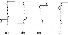
Figure 8. $dt^{k}_{c_{1},c_{2}}$ and $dt^{k}_{c_{2},c_{3}}$

When $d$ is applied to $t^{m_{\ell+1}}_{c_{2},c_{3}}$ it gives the terms depicted by (c)(d) of Figure 8. When $d$ is applied to $s^{m_{1},23}_{c_{2}}$ it gives the terms depicted by (e)(f)(g) of Figure 9. Note that (g) appears only when $m_{1}=1$.

Figure 9. $ds^{k,23}_{c_{2}}$

When $d$ is applied to $s^{m_{i},23}_{c_{2}}$, $i>1$, it gives the terms depicted by (h)(i)(j) of Figure 9. Note that (j) appears only when $m_{i}=1$. When $d$ is applied to $s^{m_{\ell},12}_{c_{2}}$ it gives the terms depicted by (k)(l)(m) of Figure 10. Note that (m) appears only when $m_{\ell}=1$.

Figure 10. $ds^{k,12}_{c_{2}}$

When $d$ is applied to $s^{m_{i},12}_{c_{2},c_{2}}$, $i<\ell$, it gives the terms depicted by (n)(o)(p) of Figure 9. Note that (p) appears only when $m_{i}=1$.

Now we observe that (b) and (g), (d) and (m), (e)+(h) and (p), (k)+(n) and (j) cancel each other.

(a) + (l) + (o) becomes $\sum_{k_{1}+k_{2}=k}s^{k_{1},13}_{c_{1}}\circ t^{k_{2},13}_{c_{1},c_{3}}$ and (c) + (f) + (i) becomes $\sum_{k_{1}+k_{2}=k}t^{k_{1},13}_{c_{1},c_{3}}\circ s^{k_{2},13}_{c_{3}}.$ We can check the sign easily. We thus verified (12.7). We can verify (12.8) in a similar way.

It is easy to calculate the energy loss of $(\{t^{k,13}_{c_{1},c_{3}}\},\{t^{k,13}_{c_{3},c_{1}},\{s^{k,13}_{c_{1}}\},\{s^{k,13}_{c_{3}}\})$ and complete the proof of Theorem 12.7. ∎

Proof of Theorem 12.12..

The proof is based on the obstruction theory and uses a construction of [FOOO1]. Let $\mathscr{C}$ be a unital completed DG-category.

Definition 12.18.

A model of $\mathscr{C}\times[0,1]$ is a unital completed DG-category $\mathfrak{C}$ with the following properties. (See [FOOO1, Definition 4.2.1].)

1. $\mathfrak{OB}(\mathscr{C})=\mathfrak{OB}(\mathfrak{C})$.

2. There exist linear and unital morphisms of completed DG-categories ${\rm Eval}_{s=0}:\mathfrak{C}\to\mathscr{C}$, ${\rm Eval}_{s=1}:\mathfrak{C}\to\mathscr{C}$ and ${\rm Incl}:\mathscr{C}\to\mathfrak{C}$. They are the identity maps for objects and preserve the finite parts.

3. ${\rm Eval}_{s=0}\circ{\rm Incl}={\rm Eval}_{s=0}\circ{\rm Incl}={\rm Identity}$.

4. The linear parts of ${\rm Eval}_{s=0}$ and ${\rm Eval}_{s=1}$ induce cochain homotopy equivalences $\mathfrak{C}(c,c^{\prime})\to\mathscr{C}(c,c^{\prime})$ for $c,c^{\prime}\in\mathfrak{OB}(\mathscr{C})$. It preserves the finite parts.

5. The map $({\rm Eval}_{s=0})_{1}\oplus({\rm Eval}_{s=1})_{1}:\mathfrak{(}a,b)\to\mathscr{C}(c,c^{\prime})\oplus\mathscr{C}(c,c^{\prime})$ is surjective. The restriction to the finite part is also surjective.

(Actually we do not use ${\rm Incl}$ in this paper.) A model of $\mathscr{C}\times[0,1]$ always exists. This is proved in the case of filtered $A_{\infty}$ algebra in [FOOO1, Subsection 4.2.1]. The construction there can be adapted to our case of unital completed filtered DG-category easily.

We next modify Maurer-Cartan equation a bit. Let $s^{k}_{c}$, $s^{k}_{c^{\prime}}$, $t^{k}_{c,c^{\prime}}$, $t^{k}_{c^{\prime},c}$, be a solution of Maurer-Cartan equation (12.7), (12.8) with energy loss $(\epsilon_{1},\epsilon_{2})$. We take

$$S^{k}_{c}=T^{k\epsilon}s^{k}_{c},\quad S^{k}_{c^{\prime}}=T^{k\epsilon}s^{k}_{c^{\prime}}\qquad T^{k}_{c,c^{\prime}}=T^{\epsilon_{1}+(k-1)\epsilon}t^{k}_{c,c^{\prime}},\qquad T^{k}_{c^{\prime},c}=T^{\epsilon_{2}+(k-1)\epsilon}t^{k}_{c^{\prime},c}.$$

They satisfy:

(12.13) $$\left\{\begin{aligned} &d(T^{k}_{c,c^{\prime}})-\sum_{\ell=1}^{k-1}S^{\ell}_{c}\circ T^{k-\ell}_{c,c^{\prime}}+\sum_{\ell=1}^{k-1}T^{k-\ell}_{c,c^{\prime}}\circ S^{\ell}_{c^{\prime}}=0\\ &d(T^{k}_{ba})-\sum_{\ell=1}^{k-1}S^{\ell}_{c^{\prime}}\circ T^{k-\ell}_{c^{\prime},c}+\sum_{\ell=1}^{k-1}T^{k-\ell}_{c^{\prime},c}\circ S^{\ell}_{c}=0\end{aligned}\right.$$

(12.14) $$\left\{\begin{aligned} &d(S^{k}_{c})-\sum_{\ell=1}^{k-1}S^{\ell}_{c}\circ S^{k-\ell}_{c}+\sum_{\ell=1}^{k}T^{1+k-\ell}_{c,c^{\prime}}\circ T^{\ell}_{c^{\prime},c}=\begin{cases}0&\text{$k\neq 1$}\\ T^{\epsilon}{\bf e}_{c}&\text{$k=1$}\end{cases}\\ &d(S^{k}_{c^{\prime}})-\sum_{\ell=1}^{k-1}S^{\ell}_{c^{\prime}}\circ S^{k-\ell}_{c^{\prime}}+\sum_{\ell=1}^{k}T^{1+k-\ell}_{c^{\prime},c}\circ T^{\ell}_{c,c^{\prime}}=\begin{cases}0&\text{$k\neq 1$}\\ T^{\epsilon}{\bf e}_{c^{\prime}}&\text{$k=1$}\end{cases}\end{aligned}\right.$$

Moreover $S^{k}_{c},S^{k}_{c^{\prime}},T^{k}_{c,c^{\prime}},T^{k}_{c^{\prime},c}$ are contained in $\mathscr{C}(c,c)$, $\mathscr{C}(c^{\prime},c^{\prime})$, $\mathscr{C}(c,c^{\prime})$, $\mathscr{C}(c^{\prime},c)$, respectively.

When $(S^{k}_{c},S^{k}_{c^{\prime}},T^{k}_{c,c^{\prime}},T^{k}_{c^{\prime},c})$ is a solution of (12.13),(12.14) then, for $\delta>0$, $(T^{2k\delta}S^{k}_{c}$, $T^{2k\delta}S^{k}_{c^{\prime}}$, $T^{(2k-1)\delta}T^{k}_{c,c^{\prime}}$, $T^{(2k-1)\delta}T^{k}_{c^{\prime},c})$ is a solution with $\epsilon$ replaced by $\epsilon+2\delta$. In case we can take $\delta$ as small as we want we say ‘raising the energy level arbitrary small amount’ to describe this process.

Now we start the proof. Let $c,c^{\prime}\in\mathfrak{OB}(\mathscr{C})$. The inequality $d_{\rm Hof,\infty}^{\mathscr{C}_{1}}(c,c^{\prime})\geq d_{\rm Hof,\infty}^{\mathscr{C}}(c,c^{\prime})$ is obvious. Here $d_{\rm Hof,\infty}^{\mathscr{C}_{1}}$, $d_{\rm Hof,\infty}^{\mathscr{C}}$ (resp. $d_{\rm Hof,\infty}^{\mathscr{C}}$) is the Hofer infinite distance of $\mathscr{C}_{1}$ (resp. $\mathscr{C}$). We will prove the opposite inequality. Suppose there exists an infinite homotopy equivalence between $c$ and $c^{\prime}$ with energy loss $\epsilon$. Then we have a solution $S^{k}_{c},S^{k}_{c^{\prime}},T^{k}_{c,c^{\prime}},T^{k}_{c^{\prime},c}$ of (12.13),(12.14).

We will construct a solution $\hat{S}^{k}_{c},\hat{S}^{k}_{c^{\prime}},\hat{T}^{k}_{c,c^{\prime}},\hat{T}^{k}_{c^{\prime},c}$ in $\mathscr{C}$ of (12.13),(12.14) with $\epsilon$ replaced by $\epsilon+2\delta_{K}$ for $k=1,\dots,K$ by induction on $K$.

1. We require ${\rm Eval}_{s=1}(\hat{S}^{k}_{c})=T^{2k\delta_{K}}S^{k}_{c}$, ${\rm Eval}_{s=1}(\hat{S}^{k}_{c^{\prime}})=T^{2k\delta_{K}}S^{k}_{c^{\prime}}$, ${\rm Eval}_{s=1}(\hat{T}^{k}_{c,c^{\prime}})=T^{2(k-1)\delta_{K}}T^{k}_{c,c^{\prime}}$, and ${\rm Eval}_{s=1}(\hat{T}^{k}_{c^{\prime},c})=T^{2(k-1)\delta_{K}}T^{k}_{c^{\prime},c}$.

2. We require ${\rm Eval}_{s=0}(\hat{S}^{k}_{c})\in\mathscr{C}_{1}(c,c)$, ${\rm Eval}_{s=0}(\hat{S}^{k}_{c^{\prime}})\in\mathscr{C}_{1}(c^{\prime},c^{\prime})$, ${\rm Eval}_{s=0}(\hat{T}^{k}_{c,c^{\prime}})\in\mathscr{C}_{1}(c,c^{\prime})$, and ${\rm Ev}_{s=0}(\hat{T}^{k}_{c^{\prime},c})\in\mathscr{C}_{1}(c^{\prime},c)$.

The construction is by induction on $K$. There are two inductive steps. The first is: given $\hat{S}^{k}_{c},\hat{S}^{k}_{c^{\prime}},\hat{T}^{k}_{c,c^{\prime}},\hat{T}^{k}_{c^{\prime},c}$ for $k<K$ we construct $\hat{T}^{K}_{c,c^{\prime}},\hat{T}^{K}_{c^{\prime},c}$ by raising the energy level arbitrary small amount. The second is: given $\hat{S}^{k}_{c},\hat{S}^{k}_{c^{\prime}}$ for $k<K$ and $\hat{T}^{k}_{c,c^{\prime}},\hat{T}^{k}_{c^{\prime},c}$ for $k\leq K$ we construct $\hat{S}^{K}_{c},\hat{S}^{K}_{c^{\prime}}$ by raising the energy level arbitrary small amount.

We describe the first inductive step. The second is entirely similar.

We put $\mathfrak{s}^{k}_{c}:={\rm Eval}_{s=0}(\hat{S}^{k}_{c})$ etc. We consider

$$OB=\sum_{\ell=1}^{K-1}\hat{S}^{\ell}_{c}\circ\hat{T}^{K-\ell}_{c,c^{\prime}}-\sum_{\ell=1}^{K-1}\hat{T}^{K-\ell}_{c,c^{\prime}}\circ\hat{S}^{\ell}_{c^{\prime}}$$

This is a cocycle and ${\rm Eval}_{s=1}(OB)=\mathfrak{M}_{1}(T^{K}_{c,c^{\prime}})$. Since ${\rm Eval}_{s=1}$ is surjective and cochain homotopy equivalence, we can show that there exists $\hat{T}^{K,\prime}_{c,c^{\prime}}\in\mathfrak{C}(c,c^{\prime})$ such that $\mathfrak{M}_{1}(\hat{T}^{K,\prime}_{c,c^{\prime}})=OB$, ${\rm Eval}_{s=1}(\hat{T}^{K,\prime}_{c,c^{\prime}})=T^{K,\prime}_{c,c^{\prime}}.$ We have

(12.15) $$\mathfrak{M}_{1}({\rm Eval}_{s=0}(\hat{T}^{K,\prime}_{c,c^{\prime}}))=\sum_{\ell=1}^{K-1}\mathfrak{s}^{\ell}_{c}\circ\mathfrak{t}^{K-\ell}_{c,c^{\prime}}-\sum_{\ell=1}^{K-1}\mathfrak{t}^{K-\ell}_{c,c^{\prime}}\circ\mathfrak{s}^{\ell}_{c^{\prime}}.$$

We denote the right hand side by $\mathfrak{ob}$. It is a cycle in $\mathscr{C}_{1}(c,c^{\prime})$. (12.15) implies that $[\mathfrak{ob}]$ is zero in $H(\mathscr{C}(c,c^{\prime}))$. Therefore by Lemma 2.15 (the almost injectivity) we may assume that $[\mathfrak{ob}]$ is zero in $H(\mathscr{C}_{1}(c,c^{\prime}))$ by raising the energy level arbitrary small amount. Therefore we have $\mathfrak{t}^{K,\prime}_{c,c^{\prime}}\in\mathscr{C}_{1}(c,c^{\prime})$ such that $\mathfrak{M}_{1}(\mathfrak{t}^{K,\prime}_{c,c^{\prime}})=\mathfrak{ob}.$ We consider ${\rm Eval}_{s=0}(\hat{T}^{K,\prime}_{c,c^{\prime}})-\mathfrak{t}^{K,\prime}_{c,c^{\prime}}.$ This is a cycle and represents an element of $H(\mathscr{C}(c,c^{\prime}))$. Therefore by Lemma 2.15 (the almost surjectivity) we may change $\mathfrak{t}^{K,\prime}_{c,c^{\prime}}$ by a cycle in $\mathscr{C}_{1}(c,c^{\prime})$ to $\mathfrak{t}^{K}_{c,c^{\prime}}$ such that ${\rm Eval}_{s=0}(\hat{T}^{K,\prime}_{c,c^{\prime}})-\mathfrak{t}^{K}_{c,c^{\prime}}$ is a coboundary $\mathfrak{M}_{1}({\rm C})$, by raising the energy level arbitrary small amount. By Definition 12.18 (5), there exists $\hat{\rm C}\in\mathfrak{C}_{1}(c,c^{\prime})$ such that ${\rm Eval}_{s=0}(\hat{\rm C})=C,$ ${\rm Eval}_{s=1}(\hat{\rm C})=0.$ Now we change $\hat{T}^{K,\prime}_{c,c^{\prime}}$ to $\hat{T}^{K}_{ab}=\hat{T}^{K,\prime}_{ab}-\mathfrak{M}_{1}(\hat{\rm C}).$ Then $\hat{T}^{K}_{c,c^{\prime}}$ has the required properties.

Thus by induction we obtain a solution $\mathfrak{s}^{k}_{c},\mathfrak{s}^{k}_{c^{\prime}},\mathfrak{t}^{k}_{c,c^{\prime}},\mathfrak{t}^{k}_{c^{\prime},c}$ of (12.13),(12.14) on $\mathfrak{C}_{1}$ by raising the energy level arbitrary small amount. The proof of Theorem 12.12 is complete. ∎

13. Equivalence of inductive limit.

Let $\mathcal{K}$ be an index set. We consider two $\mathcal{K}$ parametrized families of sequences $\mathfrak{c}_{k,(i)}=(c^{1}_{k,(i)},c^{2}_{k,(i)},\dots)$ of objects of ${\mathscr{C}}$ for $k\in\mathcal{K}$, $i=1,2$ such that

(13.1) $$d_{\rm Hof,\infty}(c^{n}_{k,(i)},c^{n+1}_{k,(i)})<\epsilon_{n},\qquad\sum_{n=1}^{\infty}\epsilon_{n}<\infty.$$

We put $\mathfrak{C}_{\mathcal{K},(i)}=\{\mathfrak{c}_{k,(i)}\mid k\in\mathcal{K}\}$ and $\mathfrak{C}^{n}_{\mathcal{K},(i)}=\{c^{n}_{k,(i)}\mid k\in\mathcal{K}\}$. By Theorem 12.16 we obtain a $\#$-unital inductive system of unital filtered $A_{\infty}$ categories $(\{\mathscr{C}(\mathfrak{C}^{n}_{\mathcal{K},(i)})\},\{\Phi^{n}_{(i)}\})$. By Proposition 11.1 and Definition 10.5, we obtain a homotopically unital completed DG-categories as the inductive limits of these inductive systems. We denote them by ${\mathscr{C}}^{\infty}(\mathfrak{C}_{\mathcal{K},(i)}):=\varinjlim\,\mathscr{C}(\mathfrak{C}^{n}_{\mathcal{K},(i)})$ and denote the unitalization of ${\mathscr{C}}^{\infty}(\mathfrak{C}_{\mathcal{K},(i)})$ by ${\mathscr{C}}^{\infty}(\mathfrak{C}_{\mathcal{K},(i)})^{+}=(\varinjlim\,\mathscr{C}(\mathfrak{C}^{n}_{\mathcal{K},(i)}))^{+}$. We use reduced version of Bar-Co-Bar resolution.

Theorem 13.1.

In the above situation we have the following two inequalities.

(13.2) $$\left\{\begin{aligned} d_{{\rm Hof},\infty}({\mathscr{C}}^{\infty}(\mathfrak{C}_{\mathcal{K},(1)})^{+},{\mathscr{C}}^{\infty}(\mathfrak{C}_{\mathcal{K},(2)})^{+})&\leq\liminf_{n\to\infty}d_{{\rm H},\infty}(\mathfrak{C}^{n}_{\mathcal{K},(1)},\mathfrak{C}^{n}_{\mathcal{K},(2)}),\\ d_{{\rm Hof}}({\mathscr{C}}^{\infty}(\mathfrak{C}_{\mathcal{K},(1)})^{+},{\mathscr{C}}^{\infty}(\mathfrak{C}_{\mathcal{K},(2)})^{+})&\leq\liminf_{n\to\infty}d_{\rm H}(\mathfrak{C}^{n}_{\mathcal{K},(1)},\mathfrak{C}^{n}_{\mathcal{K},(2)})).\end{aligned}\right.$$

Proof.

We first construct another unital inductive system of filtered $A_{\infty}$ categories $(\{\mathscr{C}^{n}_{(0)})\},\{\Phi^{n}_{(0)}\})$. Note that to define completed unital DG categories ${\mathscr{C}}^{\infty}(\mathfrak{C}_{\mathcal{K},(1)})^{+}$, ${\mathscr{C}}^{\infty}(\mathfrak{C}_{\mathcal{K},(2)})^{+}$, we defined and used $(\{\mathscr{C}(\mathfrak{C}^{n}_{\mathcal{K},(i)})\},\{\Phi^{n}_{(i)}\})$ for $i=1,2$. We made two choices to define it.

1. We take an infinite homotopy equivalence between $c_{k,(i)}^{n}$ and $c_{k,(i)}^{n+1}$ for each $n$ and $k$. (We used it to obtain $\Phi_{(i)}^{n}$ by Lemma 12.17.)

2. We also take a splitting (10.2) to obtain a unital filtered $A_{\infty}$ functor from a $\#$-homotopical unital filtered $A_{\infty}$ functor.

We fix these two choices for $i=1,2$. We put $\mathscr{C}_{(0)}^{n}={\mathscr{C}}^{(n)}(\mathfrak{OB}(\mathscr{C}_{(1)}^{n})\sqcup\mathfrak{OB}(\mathscr{C}_{(2)}^{n}))$. Note that we take disjoint union $\sqcup$ and not the union. In other words in the case when $\mathfrak{OB}(\mathscr{C}_{(1)}^{n})\cap\mathfrak{OB}(\mathscr{C}_{(2)}^{n})\neq\emptyset$ we still regard the elements of the intersection as two different elements.

Now the choices $(*)(**)$ made for $i=1,2$ induce the choices $(*)(**)$ for $i=0$. Using them we obtain a unital inductive system of filtered $A_{\infty}$ categories $(\{\mathscr{C}^{n}_{(0)})\},\{\Phi^{n}_{(0)}\})$.

Because of our choice we obtain a fully faithful embeddings of unital filtered $A_{\infty}$ categories $\Psi_{i}^{n}:\mathscr{C}(\mathfrak{C}^{n}_{\mathcal{K},(i)})\to\mathscr{C}_{(0)}^{n}$ with energy loss $0$ for $i=1,2$, such that

(13.3) $$\Phi_{(0)}^{n}\circ\Psi_{i}^{n}=\Psi_{i}^{n+1}\circ\Phi_{(i)}^{n}.$$

for $i=1,2$. We emphasis that this is an exact equality. Therefore the second inequality is a consequence of Lemma 11.6.

The proof of the first inequality is mostly the same. During the proof of Lemma 11.6 we obtained ${\mathscr{C}}^{\infty}(\mathfrak{C}_{\mathcal{K},(0)})^{+}:=\varinjlim\,\mathscr{C}_{(0)}^{n}$ and an almost homotopy equivalent injection to this completed DG-category from ${\mathscr{C}}^{\infty}(\mathfrak{C}_{\mathcal{K},(i)})^{+}$, for $i=1,2$ (Lemma 11.7). It suffices to estimate $d_{{\rm Hof},\infty}(\mathfrak{c}_{k,(1)},\mathfrak{c}_{k,(2)})$. Here $\mathfrak{c}_{k,(1)},\mathfrak{c}_{k,(2)}$ are regarded as objects of ${\mathscr{C}}^{\infty}(\mathfrak{C}_{\mathcal{K},(0)})^{+}$.

By construction there exists a unital filtered $A_{\infty}$ functor $(\Upsilon^{\infty,n})^{+}:\mathscr{C}_{(0)}^{n}\to{\mathscr{C}}^{\infty}(\mathfrak{C}_{\mathcal{K},(0)})^{+}$ of energy loss $\epsilon^{\prime}_{n}$ such that $\lim_{n\to\infty}\epsilon^{\prime}_{n}=0$. Let $\rho_{n}=d_{{\rm H},\infty}(\mathfrak{C}^{n}_{\mathcal{K},(1)},\mathfrak{C}^{n}_{\mathcal{K},(2)})$ Note $\Upsilon^{\infty,n}_{\rm ob}(c^{n}_{\mathcal{K},(i)})=\mathfrak{c}_{k,(i)}$. Therefore by Lemma 12.5 we have $d_{{\rm Hof},\infty}(\mathfrak{c}_{k,(1)},\mathfrak{c}_{k,(2)})\leq\rho_{n}+\epsilon^{\prime}_{n}.$ Since $\epsilon^{\prime}_{n}$ is arbitrary small the first inequality holds. ∎

We remark that the above proof implies the next:

Proposition 13.2.

The limit completed DG-category ${\mathscr{C}}^{\infty}(\mathfrak{C}_{\mathcal{K},(i)})^{+}$ is independent of the choices $(*)$, $(**)$ up to equivalence.

Corollary 13.3.

We consider a $\mathcal{K}$ parametrized family of sequences $\mathfrak{c}_{k}=(c^{1}_{k},c^{2}_{k},\dots)$ of objects of ${\mathscr{C}}$ for $k\in\mathcal{K}$ such that $d_{\rm Hof,\infty}(c^{n}_{k},c^{n+1}_{k})<\epsilon_{n},$ $\sum_{n=1}^{\infty}\epsilon_{n}<\infty.$ We put $\mathfrak{C}^{n}_{\mathcal{K}}=\{c^{n}_{k}\mid k\in\mathcal{K}\}$. Then the sequence $\mathscr{C}(\mathfrak{C}^{n}_{\mathcal{K}})^{+}$, $n=1,2,\dots$ converges to $\varinjlim\,\mathscr{C}(\mathfrak{C}^{n}_{\mathcal{K}})^{+}$ in Gromov-Hausdorff infinite distance.

Proof.

We put $c^{n}_{k,(2)}=c^{m}_{k,(2)}$ for $n>m$ and $c^{n}_{k,(2)}=c^{n}_{k,(2)}$ for $n\leq m$. We also put $c^{n}_{k,(1)}=c^{n}_{k}$. Then Theorem 13.1 implies

(13.4) $$d_{{\rm Hof}}(\varinjlim\,\mathscr{C}(\mathfrak{C}^{n}_{\mathcal{K}})^{+},\mathscr{C}(\mathfrak{C}^{m}_{\mathcal{K}})^{+})\leq\liminf_{n\to\infty}d_{H,\infty}(\mathfrak{C}^{n}_{\mathcal{K}},\mathfrak{C}^{m}_{\mathcal{K}}).$$

The corollary follows from this inequality. ∎

Remark 13.4.

Let $(\{\mathscr{C}^{n}_{(i)}\},\{\Phi_{(i)}^{n}\})$ be a unital inductive system of filtered $A_{\infty}$ categories, for $i=1,2$. The author does not know whether

$$d_{\rm GH,\infty}(\varinjlim\,\mathscr{C}^{n}_{(1)},\varinjlim\,\mathscr{C}^{n}_{(2)})\leq\liminf_{n\to\infty}d_{\rm GH,\infty}(\mathscr{C}^{n}_{(1)},\mathscr{C}^{n}_{(2)})$$

holds or not. If one tries to prove it then it seems necessary to generalize Lemma 11.6 so that the exact equality (11.3) is relaxed to a certain ‘homotopical commutativity’.

14. Spectre dimension and Gromov-Hausdorff distance.

In this section we study the relation of spectre dimension of the cohomlology group and Gromov-Hausdorff distance. Let $\mathscr{C}_{1}$ and $\mathscr{C}_{2}$ be filtered $A_{\infty}$ category (gapped case) or completed DG-category (the case of the limit). We assume that $d_{\rm GH,\infty}(\mathscr{C}_{1},\mathscr{C}_{2})<\epsilon$ and take $\mathscr{C}$ as in Definition 12.10.

Theorem 14.1.

Let $a,b\in\mathfrak{OB}(\mathscr{C}_{1})$ and $a^{\prime},b^{\prime}\in\mathfrak{OB}(\mathscr{C}_{2})$ such that

$$d_{\rm Hof,\infty}(a,a^{\prime})<\epsilon_{,}\qquad d_{\rm Hof,\infty}(b,b^{\prime})<\epsilon.$$

Let $H_{1}(a,b)=H(\mathscr{C}_{1}(a,b),\mathfrak{m}_{1})$, $H_{2}(a^{\prime},b^{\prime})=H(\mathscr{C}_{2}(a^{\prime},b^{\prime}),\mathfrak{m}_{1})$. Then for $2\epsilon\leq\lambda$

$$f(\lambda;H_{1}(a,b))\leq f(\lambda-2\epsilon;H_{2}(a^{\prime},b^{\prime})),\qquad f(\lambda;H_{2}(a^{\prime},b^{\prime}))\leq f(\lambda-2\epsilon;H_{1}(a,b)).$$

In particular if $d_{\rm Hof,\infty}(a,a^{\prime})=d_{\rm Hof,\infty}(b,b^{\prime})=0$ then $H(\mathscr{C}_{1}(a,b),\mathfrak{m}_{1})$ is almost isomorphic to $H(\mathscr{C}_{2}(a^{\prime},b^{\prime}),\mathfrak{m}_{1})$.

Theorem 14.1, Proposition 13.2 and Corollary 13.3 imply the next:

Corollary 14.2.

Suppose that we are in the situation of Proposition 13.2. Then $H(\mathscr{C}^{\infty}(\mathfrak{c}_{k,(1)},\mathfrak{c}_{k^{\prime},(1}),\mathfrak{m}_{1})$ is almost isomorphic to $H(\mathscr{C}^{\infty}(\mathfrak{c}_{k,(2)},\mathfrak{c}_{k^{\prime},(2)}),\mathfrak{m}_{1})$.

In the situation of Corollary 13.3. We put $H_{\infty}=H(\mathscr{C}^{\infty}(\mathfrak{c}_{k},\mathfrak{c}_{k^{\prime}}),\mathfrak{m}_{1})$ and $H_{n}=H(\mathscr{C}^{n}(c_{k},c_{k^{\prime}}),\mathfrak{m}_{1})$. Then, there exists $\epsilon_{n}$ which converges to $0$ and such that

$$f(\lambda;H_{\infty})\leq f(\lambda-\epsilon_{n};H_{n}),\qquad f(\lambda;H_{n})\leq f(\lambda-\epsilon_{n};H_{\infty}).$$

The proof of Theorem 14.1 uses Lemma 2.12, which we now prove.

Proof of Lemma 2.12.

Let $\varphi:V_{1}\to V_{2}$ be an almost isomorphism between divisible filtered $\Lambda_{0}$ modules. Let $W\in V_{2}$ be a finitely generated submodule of $F^{\lambda}V_{2}$. Let $x_{i}\in V_{2}$, $i=1,\dots,m$ be its generator. Note that $T^{-\lambda}x_{i}\in V_{2}$ exists by divisibility. For $\epsilon>0$, there exists $y^{\prime}_{i}\in V_{1}$ such that $T^{\epsilon-\lambda}x_{i}=\varphi(y^{\prime}_{i})$. We put $y_{i}=T^{\lambda-\epsilon}y^{\prime}_{i}$. Let $W^{\prime}$ be a submodule of $F^{\lambda-\epsilon}V_{1}$ generated by $y_{i}$, $i=1,\dots,m$. Then $\varphi(W^{\prime})=W$.

By definition, $W^{\prime}$ is generated by $m^{\prime}$ elements $z_{1},\dots,z_{m^{\prime}}$ with $m^{\prime}=f(\lambda-\epsilon;V_{1})$. Therefore $W$ is generated by $\varphi(z_{1}),\dots,\varphi(z_{m^{\prime}})$. We have proved $f(\lambda;V_{2})\leq\lim_{\epsilon>0,\epsilon\to 0}f(\lambda-\epsilon;V_{1}).$

We next prove an inequality of opposite direction. Since $f(\lambda;V_{1})$ is an integer valued non-increasing function, there exists a discrete set $S$ such that if $\lambda\notin S$ then there exists $\lambda^{\prime}>\lambda$ such that $f(\lambda;V_{1})=f(\lambda^{\prime};V_{1})$. We take such $\lambda$, $\lambda^{\prime}$. We put $\epsilon=\lambda^{\prime}-\lambda$. Let $W\subset F^{\lambda^{\prime}}V_{1}$ be a finitely generated submodule such that the minimal number of generators of $W$ is $m=f(\lambda^{\prime};V_{1})$. By divisibility there exists $W_{1}\subset F^{\lambda}V_{1}$ such that $T^{\epsilon}W_{1}=W$ and $W_{1}$ is finitely generated. Let $\{x_{1},\dots,x_{m}\}$ be a generator of $W_{1}$. Let $W^{\prime}=\varphi(W_{1})$. Then $W^{\prime}$ is a finitely generated submodule of $F^{\lambda}V_{2}$. Therefore it is generated by $m^{\prime}=f(\lambda;V_{2})$ elements. Suppose it is generated by $\varphi(y_{1}),\dots,\varphi(y_{m^{\prime}})$. There exists $a_{ij}\in\Lambda_{0}$ such that $\varphi\left(x_{i}-\sum_{j}a_{ij}y_{j}\right)=0$ for $i=1,\dots,m$. Since $\varphi$ is almost injective, it implies $T^{\epsilon}x_{i}=\sum_{j}T^{\epsilon}a_{ij}y_{j}.$ Therefore $W$ is generated by $m^{\prime}$ elements. We have proved $f(\lambda;V_{1})\leq f(\lambda;V_{2}),$ for $\lambda\notin S$. The proof of Lemma 2.12 is complete. ∎

Lemma 14.3.

Let $(C_{1},d_{1}),(C_{2},d_{2})$ be filtered cochain complexes over $\Lambda_{0}$ and $\varphi:(C_{1},d_{1})\to(C_{2},d_{2})$ a cochain homotopy equivalence with energy loss $\epsilon$ in the sense of Definition 4.6. Then

$$f(\lambda;H(C_{1},d_{1}))\leq f(\lambda-\epsilon;H(C_{2},d_{2})),\qquad f(\lambda;H(C_{2},d_{2}))\leq f(\lambda-\epsilon;H(C_{1},d_{1})).$$

for $\lambda\geq\epsilon$.

Proof.

By definition there exists $\epsilon_{1}$, $\epsilon_{2}$ with $\epsilon_{1}+\epsilon_{2}=\epsilon$ and $\psi:(C_{1},d_{1})\to(C_{2},d_{2})$ such that $T^{\epsilon_{1}}\varphi$ and $T^{\epsilon_{2}}\psi$ preserves the energy filtration and $T^{\epsilon_{2}}\psi\circ T^{\epsilon_{1}}\varphi$ and $T^{\epsilon_{1}}\varphi\circ T^{\epsilon_{2}}\psi$ are cochain homotopic to $T^{\epsilon}$, (by cochain homotopy which preserves filtrations). Thus there exist $h=(T^{\epsilon_{1}}\varphi)_{*}:H(C_{1},d_{1})\to H(C_{2},d_{2})$ and $g=(T^{\epsilon_{2}}\psi)_{*}:H(C_{2},d_{2})\to H(C_{1},d_{1})$ such that $h\circ g=T^{\epsilon}$ and $g\circ h=T^{\epsilon}$.

Let $W\subset F^{\lambda}H(C_{1},d_{1})$ be a finitely generated submodule. By divisibility, there exists $W_{0}\subset F^{\lambda-\epsilon}H(C_{1},d_{1})$ such that $W=T^{\epsilon}W_{0}$. Since $h(W_{0})\subset F^{\lambda-\epsilon}H(C_{2},d_{2})$ it is generated by $f(\lambda-\epsilon;H(C_{2},d_{2}))$ elements. Therefore $W=gh(W_{0})$ is generated by $f(\lambda-\epsilon;H(C_{2},d_{2}))$ elements. We have proved $f(\lambda;H(C_{1},d_{1}))\leq f(\lambda-\epsilon;H(C_{2},d_{2}))$. We can prove the other inequality by exchanging the role of $g$ and $h$. ∎

Theorem 14.1 follows from Theorem 4.7 and Lemmas 2.12 and 14.3.

Remark 14.4.

The proof of Lemma 14.3 is mostly the same as the proof of [FOOO1, Lemma 6.5.31] which was used to prove (1.2). A similar argument is used in the study of persistence modules. See for example [PRSZ, Section 2.2].

The proof of Theorem 12.13.

By Theorem 12.12 $\mathfrak{OB}(\mathscr{C}_{1})$ and $\mathfrak{OB}(\mathscr{C}_{2})$ are subspaces of $\mathfrak{OB}(\mathscr{C})$. The Hausdorff distance between them in $\mathfrak{OB}(\mathscr{C})$ is zero. Using the assumption that $\mathfrak{OB}(\mathscr{C}_{i})$ is complete and Hausdorff it implies that $\mathfrak{OB}(\mathscr{C}_{1})$ is isometric to $\mathfrak{OB}(\mathscr{C}_{2})$. The second half then follows from Theorem 14.1. ∎

15. The proof of Theorem 1.3.

In this section we prove Theorem 1.3. Let $\{\mathbb{L}^{n}\}\in\mathfrak{Lag}^{K}_{\rm trans}$, $n=1,2,\dots$ be a Cauchy sequence with respect to Hofer distance. We first consider the following situation.

Definition 15.1.

We say that $\{\mathbb{L}^{n}\}$ is a strongly transversal sequence if $\mathbb{L}^{n}\sqcup\mathbb{L}^{n+1}\in\mathfrak{Lag}^{2K}_{\rm trans}$ holds for each $n$.

Step 1. Let $\{\mathbb{L}^{n}\}$ be a strongly transversal Cauchy sequence. We first fix a compatible almost complex structure. We also choose a system of data needed to define the filtered $A_{\infty}$ category $\mathfrak{F}(\mathbb{L}^{n})$, that is, Kuranishi structures on the moduli spaces of pseudo-holomorphic disks, strips and polygons involved and CF-perturbations to obtain virtual fundamental chains. We denote this choice by $\Xi^{n}$. We have thus obtained $\mathfrak{F}(\mathbb{L}^{n})$.

By [Fu4] we can take those Kuranishi structures and CF-perturbations so that they are compatible with the forgetful maps of the boundary marked points (other than $0$-th marked point). Then the differential 0-form $1$ of each $L\in\mathbb{L}^{n}$ becomes a strict unit. We next define $\mathfrak{F}(\mathbb{L}^{n}\sqcup\mathbb{L}^{n+1})$. Note that the moduli spaces of pseudo-holomorphic disks, strips and polygons needed to define this filtered $A_{\infty}$ category have Kuranishi structures. We construct the Kuranishi structures by induction on energy and complexity of the source. Its boundary is a union of the fiber products of moduli spaces of pseudo-holomorphic disks, strips and polygons which appear in the definition of $\mathfrak{F}(\mathbb{L}^{n})$ and $\mathfrak{F}(\mathbb{L}^{n+1})$ or those which appeared in the earlier steps of induction. Therefore the Kuranishi structures and CF-perturbations at the boundary of the moduli spaces are already given by $\Xi^{n}$, $\Xi^{n+1}$ or by induction hypothesis. By [FOOO4, FOOO6] we can obtain Kuranshi structures on those moduli spaces of pseudo-holomorphic disks, strips and polygons so that they are compatible each other at the boundary and corners, and also for the part of the moduli space of disks, strips and polygons appearing in the construction of $\mathfrak{F}(\mathbb{L}^{n})$ and $\mathfrak{F}(\mathbb{L}^{n+1})$ it coincides with $\Xi^{n}$ and $\Xi^{n+1}$. Then by [FOOO5, Chapter 17], we obtain a system of CF-perturbations so that they are compatible with each other and also with the CF-perturbations given in $\Xi^{n}$ and $\Xi^{n+1}$. We denote this system of Kuranishi structures and CF-perturbations by $\Xi^{n,n+1}$.

We thus obtained $\mathfrak{F}(\mathbb{L}^{n}\sqcup\mathbb{L}^{n+1})$. By construction $\mathfrak{F}(\mathbb{L}^{n})$ and $\mathfrak{F}(\mathbb{L}^{n+1})$ are its full subcategories. In fact, since we extend the given system of Kuranishi structures and CF-perturbations to the one we need to obtain this filtered $A_{\infty}$ category, the structure operations of $\mathfrak{F}(\mathbb{L}^{n}\cup\mathbb{L}^{n+1})$ coincide with the structure operations of $\mathfrak{F}(\mathbb{L}^{n})$ or $\mathfrak{F}(\mathbb{L}^{n+1})$ as far as the morphisms between the objects in the latter categories concern.

We put $\epsilon_{n}=d_{\rm Hof}(\mathbb{L}^{n},\mathbb{L}^{n+1})$. Then by Corollary 12.15 the Haudorff distance (with respect to the Hofer infinite distance) of $\mathfrak{OB}(\mathfrak{F}(\mathbb{L}^{n}))$ and $\mathfrak{OB}(\mathfrak{F}(\mathbb{L}^{n+1}))$ in $\mathfrak{OB}(\mathbb{L}^{n}\sqcup\mathbb{L}^{n+1})$ is not greater than $\epsilon_{n}$. Therefore by Theorem 12.16 we obtain a $\#$-unital filtered $A_{\infty}$ functor $\Phi^{n}:\mathfrak{OB}(\mathfrak{F}(\mathbb{L}^{n}))\to\mathfrak{OB}(\mathfrak{F}(\mathbb{L}^{n+1}))$ with energy loss $\epsilon_{n}$. Thus we obtain a $\#$-unital inductive system of filtered $A_{\infty}$ categories $(\{\mathfrak{F}(\mathbb{L}^{n})\},\{\Phi^{n}\})$. Therefore we obtain a unital completed DG-category $\varinjlim\,\mathfrak{F}(\mathbb{L}^{n})$. This depends on the choices $\{\Xi^{n}\},\{\Xi^{n,n+1}\}$ and $(*)$, $(**)$ appearing in the proof of Theorem 13.1.

Definition 15.2.

Let $\{\mathbb{L}^{n,i}\}$ be a strongly transversal sequence for $i=1,2$. We say a pair $(\{\mathbb{L}^{n,1}\},\{\mathbb{L}^{n,2}\})$ is strongly transversal if for any $n$ the set of Lagrangian submanifolds $\mathbb{L}^{n,1}\cup\mathbb{L}^{n+1,1}\cup\mathbb{L}^{n,2}\cup\mathbb{L}^{n+1,2}$ is an element of $\mathfrak{Lag}^{4K}_{\rm trans}$.

Step 2. Let $(\{\mathbb{L}^{n,1}\},\{\mathbb{L}^{n,2}\})$ be a strongly transversal pair of strongly transversal Cauchy sequences. We fix choices of $\{\Xi^{n,i}\},\{\Xi^{n,n+1,i}\}$ for $i=1,2$ and $(*)$, $(**)$. We then obtain $\varinjlim\,\mathfrak{F}(\mathbb{L}^{n,i})$ for $i=1,2$.

Lemma 15.3.

In this situation we have:

(15.1) $$d_{\rm GH,\infty}(\varinjlim\,\mathfrak{F}(\mathbb{L}^{n,1}),\varinjlim\,\mathfrak{F}(\mathbb{L}^{n,2}))\leq\liminf_{n\to\infty}d_{\rm Hof}(\mathbb{L}^{1},\mathbb{L}^{2}).$$

In the case the right hand side is $0$, the inductive limit $\varinjlim\,\mathfrak{F}(\mathbb{L}^{n,1})$ is equivalent to $\varinjlim\,\mathfrak{F}(\mathbb{L}^{n,2})$.

Proof.

We first construct a filtered $A_{\infty}$ category $\mathfrak{F}(\mathbb{L}^{n,1}\sqcup\mathbb{L}^{n,2})$. The construction is the same as the case of $\mathfrak{F}(\mathbb{L}^{n}\sqcup\mathbb{L}^{n+1})$. Namely we can extend the given system of Kuranishi structures and CF-perturbations $\Xi^{n,1}$, $\Xi^{n,2}$ to $\Xi^{n,1,2}$. Therefore $\mathfrak{F}(\mathbb{L}^{n,1})$ and $\mathfrak{F}(\mathbb{L}^{n,2})$ are full subcategory of $\mathfrak{F}(\mathbb{L}^{n,1}\sqcup\mathbb{L}^{n,2})$. We next perform the same construction to obtain a system of Kuranishi structures and CF-perturbations $\Xi^{n,n+1,1,2}$ and define $\mathfrak{F}(\mathbb{L}^{n,1}\sqcup\mathbb{L}^{n+1,1}\sqcup\mathbb{L}^{n,2}\sqcup\mathbb{L}^{n+1,2})$. The four filtered $A_{\infty}$ categories $\mathfrak{F}(\mathbb{L}^{n,1}\sqcup\mathbb{L}^{n,2})$, $\mathfrak{F}(\mathbb{L}^{n+1,1}\sqcup\mathbb{L}^{n+1,2})$, $\mathfrak{F}(\mathbb{L}^{n,1}\sqcup\mathbb{L}^{n+1,1})$, $\mathfrak{F}(\mathbb{L}^{n,2}\sqcup\mathbb{L}^{n+1,2})$, are full subcategories of $\mathfrak{F}(\mathbb{L}^{n,1}\sqcup\mathbb{L}^{n+1,1}\sqcup\mathbb{L}^{n,2}\sqcup\mathbb{L}^{n+1,2})$. Using again Corollary 12.15 and Theorem 12.16 we obtain a $\#$-unital filtered $A_{\infty}$ functor

$$\Phi^{n,0}:\mathfrak{F}(\mathbb{L}^{n,1}\sqcup\mathbb{L}^{n,2})\to\mathfrak{F}(\mathbb{L}^{n+1,1}\sqcup\mathbb{L}^{n+1,2})$$

with energy loss $\epsilon_{n}$. Here $\epsilon_{n}=\max(d_{\rm Hof}(\mathbb{L}^{n,1},\mathbb{L}^{n+1,1}),d_{\rm Hof}(\mathbb{L}^{n,2},\mathbb{L}^{n+1,2}))$.

Let $\Psi_{i}^{n}:\mathfrak{F}(\mathbb{L}^{n,i})\to\mathfrak{F}(\mathbb{L}^{n,1}\sqcup\mathbb{L}^{n,2})$ be canonical embedding as full subcategories, for $i=1,2$. By construction we have

(15.2) $$\Phi^{n,0}\circ\Psi_{i}^{n}=\Psi_{i}^{n+1}\circ\Phi^{n,i}.$$

This is an exact equality. The rest of the proof is the same as the proof of Lemma 11.6 and Theorem 13.1. ∎

Step 3. Let $\mathbb{L}$ be an element of the completion $\overline{\mathfrak{Lag}^{K}}$ of $\mathfrak{Lag}^{K}$. We first observe that there exists a strongly transversal Cauchy sequence $\{\mathbb{L}^{n}\}$ which converges to $\mathbb{L}$. We next observe that for two strongly transversal Cauchy sequences $\{\mathbb{L}^{n,i}\}$, $i=1,2$ converging to $\mathbb{L}$, there exists a third strongly transversal Cauchy sequence $\{\mathbb{L}^{n,3}\}$ converging to $\mathbb{L}$, such that the pairs $(\{\mathbb{L}^{n,1}\},\{\mathbb{L}^{n,3}\})$ and $(\{\mathbb{L}^{n,2}\},\{\mathbb{L}^{n,3}\})$ are both strongly transversal. Using Lemma 15.3 twice we conclude that $\varinjlim\,\mathfrak{F}(\mathbb{L}^{n,1})$ is equivalent to $\varinjlim\,\mathfrak{F}(\mathbb{L}^{n,2})$. Thus by using the limit we obtain $\mathfrak{F}(\mathbb{L})$ which is well-defined up to equivalence.

Step 4. Let $\mathbb{L}_{m}\in\overline{\mathfrak{Lag}^{K}}$ and $\mathbb{L}_{m}$, $m=1,2,\dots$ be a Cauchy sequence. We will prove that $\mathfrak{F}(\mathbb{L}_{m})$ converges with respect to the Gromov-Hausdorff infinite distance. We put $\epsilon^{\prime}_{m}=\sum_{\ell\geq m}d_{\rm Hof}(\mathbb{L}_{\ell},\mathbb{L}_{\ell+1})$. We observe that there exists a $n,m\in{\mathbb{Z}}_{+}$ parametrized family of objects $\mathbb{L}^{n}_{m}\in\mathfrak{Lag}^{K}_{\rm trans}$ such that:

1. $d_{\rm Hof}(\mathbb{L}_{m},\mathbb{L}^{n}_{m})<1/n$,

2. For any positive integers $m,m^{\prime},m^{\prime\prime}$ we have $\mathbb{L}^{n}_{m}\cup\mathbb{L}^{n+1}_{m}\sqcup\mathbb{L}^{n}_{m^{\prime}}\sqcup\mathbb{L}^{n+1}_{m^{\prime}}\sqcup\mathbb{L}^{n}_{m^{\prime\prime}}\sqcup\mathbb{L}^{n+1}_{m^{\prime\prime}}\in\mathfrak{Lag}^{6K}_{\rm trans}$.

The existence of such $\mathbb{L}^{n}_{m}$ is easy to prove.

We consider the sequence $\{\mathbb{L}^{n}_{n}\}$. It is a Cauchy sequence and is strongly transversal. Therefore we obtain the limit $\varinjlim\,\mathfrak{F}(\mathbb{L}^{n}_{n})$. We consider another sequence, $\{\mathbb{L}^{n}_{m}\}$ for a fixed $m$. Then by item (2), the pair $(\{\mathbb{L}^{n}_{m}\},\{\mathbb{L}^{n}_{n}\})$ is transversal. Therefore by Lemma 15.3 we have $d_{\rm GH,\infty}(\varinjlim\,\mathfrak{F}(\mathbb{L}^{n}_{n}),\mathbb{L}_{m})\leq\epsilon^{\prime}_{m}.$ Therefore $\mathfrak{F}(\mathbb{L}_{m})$ converges to $\varinjlim\,\mathfrak{F}(\mathbb{L}^{n}_{n})$ by Gromov-Hausdorff infinite distance. The uniqueness of the limit up to equivalence can be proved in the same way as Step 3.

Step 5. We take a compatible almost complex structure $J$ at the beginning of the construction. We will prove that $\mathfrak{F}(\mathbb{L})$ is independent of the choice of $J$ up to equivalence. Let $J_{0},J_{1}$ be two compatible almost complex structures. We take a path $\mathcal{J}=\{J_{t}\}$ of compatible almost complex structures joining them. We may assume that $J_{t}=J_{0}$ for sufficiently small $t$ and $J_{t}=J_{1}$ if $1-t$ is sufficiently small.

Let $\mathbb{L}^{n}\in\mathfrak{Lag}^{K}_{\rm trans}$. We take choices $\Xi_{0}^{n}$ (resp. $\Xi_{1}^{n}$), that is, Kuranishi structures and CF-perturbations of the moduli spaces of pseudo holomorphic disks, strips and polygons, with respect to the almost complex structure $J_{0}$ (resp $J_{1}$) and obtain $\mathfrak{F}(\mathbb{L}^{n};J_{0})$, $\mathfrak{F}(\mathbb{L}^{n};J_{1})$.

We consider the disjoint union $(\mathbb{L}^{n}\times\{0\})\sqcup(\mathbb{L}^{n}\times\{1\})$ of two copies of $\mathbb{L}^{n}$. We put $\widehat{\mathbb{L}}^{n}=(\mathbb{L}^{n}\times\{0\})\sqcup(\mathbb{L}^{n}\times\{1\})$. For an element $L$ of $\mathbb{L}^{n}$ we write $L(0)$ (resp. $L(1)$) when we regard it as an object of $\mathfrak{F}(\mathbb{L}^{n};J_{0})$ (resp. $\mathfrak{F}(\mathbb{L}^{n};J_{1})$).

Using $J_{t}$ and extending the given data $\Xi^{n}$, $\Xi^{\prime n}$ we obtain a pseudo-isotopy between $\mathfrak{F}(\mathbb{L}^{n};J_{0})$ and $\mathfrak{F}(\mathbb{L}^{n};J_{1})$, which we write $\mathfrak{F}(\mathbb{L}^{n};\mathcal{J})$. Roughly speaking this is the following object. For $L\neq L^{\prime}$, $L,L^{\prime}\in\mathbb{L}^{n}$, the morphism complex $CF(L,L^{\prime};J_{j})$ (for $j=0,1$) between them is a free $\Lambda_{0}$ module

$$CF(L,L^{\prime};J_{j})=\bigoplus_{p\in L\cap L^{\prime}}\Lambda_{0}[p]$$

generated by the intersection points. We change it to

$$CF(L,L^{\prime};\mathcal{J})=\bigoplus_{p\in L\cap L^{\prime}}\Omega([0,1])[p]\,\widehat{\otimes}\,\Lambda_{0}.$$

Here $\Omega([0,1])$ is the de Rham complex of the interval.

For $L=L^{\prime}\in\mathbb{L}^{n}$, we put

$$CF(L,L;\mathcal{J})=\Omega(L\times[0,1])\widehat{\otimes}\Lambda_{0}.$$

We use the union of the moduli spaces of $J_{t}$-disks, strips and polygons for $t\in[0,1]$. On these spaces we can define Kuranishi structures and CF perturbations extending $\Xi_{0}^{n}$, $\Xi^{n}_{1}$, which we denote by $\Xi_{01}^{n}$. See [FOOO4, FOOO6] for the detail of this construction.

This filtered $A_{\infty}$ category is curved. (The operator $\mathfrak{m}_{0}$ may be non-zero.) Using bounding cochains we can eliminate $\mathfrak{m}_{0}$ and obtain a strict filtered $A_{\infty}$ category which we denote by $\mathfrak{F}(\mathbb{L}^{n};\mathcal{J})$.

The pullbacks of differential forms by the inclusions $\{0\}\to[0,1]$, $\{1\}\to[0,1]$ define filtered $A_{\infty}$ functors (of energy loss $0$) $\mathfrak{J}^{n}_{0}:\mathfrak{F}(\mathbb{L}^{n};\mathcal{J})\to\mathfrak{F}(\mathbb{L}^{n};J_{0})$, $\mathfrak{J}^{n}_{1}:\mathfrak{F}(\mathbb{L}^{n};\mathcal{J})\to\mathfrak{F}(\mathbb{L}^{n};J_{1})$ which are homotopy equivalences.

To use the filtered $A_{\infty}$ category $\mathfrak{F}(\mathbb{L}^{n};\mathcal{J})$ to prove that $\mathfrak{F}(\mathbb{L}^{n};J_{0})$ is equivalent to $\mathfrak{F}(\mathbb{L}^{n};J_{1})$, we invert the arrows of $\mathfrak{J}^{n}_{j}$ as follows. We first review the structure operations $\mathfrak{M}_{k}$ of $\mathfrak{F}(\mathbb{L}^{n};\mathcal{J})$.

Let $h_{i}$ be a differential form on $[0,1]\times(L\cap L^{\prime})$ or $[0,1]\times L$. Let $t$ be the standard coordinate of $[0,1]$. We write $h_{i}$ as $h_{i}=h_{i}^{0}+dt\wedge h_{i}^{1}$ where $h_{i}^{0}$, $h_{i}^{1}$ are smoothly $t$-dependent family of smooth differential forms on $L$ or on $L\cap L^{\prime}$. (In case $L\neq L^{\prime}$ the latter is a finite set.) Then

(15.3) $$\mathfrak{M}_{k}(h_{1},\dots,h_{k})$$

$$=\mathfrak{m}^{\sharp}_{k}(h^{0}_{1},\dots,h^{0}_{k})+dt\wedge\mathfrak{c}_{k}(h^{0}_{1},\dots,h^{0}_{k})$$

$$\,\,\,\,\,+dt\wedge\sum_{i=1}^{k}(-1)^{1+\deg^{\prime}h^{0}_{1}+\dots+\deg^{\prime}h^{0}_{i-1}}\mathfrak{m}^{\sharp}_{k}(h^{0}_{1},\dots,h^{1}_{i},\dots,h^{0}_{k})$$

for $k\neq 1$ and

(15.4) $$\mathfrak{M}_{1}(h)= \mathfrak{m}^{\sharp}_{1}(h^{0})-\frac{\partial h^{0}}{\partial t}+dt\wedge\mathfrak{c}_{1}(h^{0})-dt\wedge\mathfrak{m}^{\sharp}_{1}(h^{1})$$

where $\mathfrak{m}^{\sharp}_{k}$ and $\mathfrak{c}_{k}$ are smoothly $t$-depedent family of operators with smooth Schwartz kernels, except $\mathfrak{m}_{1}^{\sharp}$ contains the de Rham differential $d$ on $L$ and $\mathfrak{m}_{2}^{\sharp}$ contains the cup product. (They do not have smooth Schwartz kernels but their $t$ derivatives are $0$.) (See [FOOO5, Section 22.3].)

A filtered $A_{\infty}$ functor $\Psi^{n,c}_{0}:\mathfrak{F}_{c}(\mathbb{L}^{n};J_{0})\to\mathfrak{F}_{c}(\mathbb{L}^{n};\mathcal{J})$ we look for is of the form

$$(\Psi^{n,c}_{0})_{k}(g_{1},\dots,g_{k})=(\Psi^{n,c}_{0})^{0}_{k}(g_{1},\dots,g_{k})+dt\wedge(\Psi^{n,c}_{0})^{1}_{k}(g_{1},\dots,g_{k}),$$

where $g_{i}$ are differential forms on $L$ or on $L\cap L^{\prime}$ and $(\Psi^{n,c}_{0})^{0}_{k}$, $(\Psi^{n,c}_{0})^{1}_{k}$ have smooth Schwartz kernels, except $(\Psi^{n,c}_{0})^{0}_{1}$ contains the identity map. (Note that the right hand side is a differential form on $[0,1]\times L$ or $[0,1]\times(L\cap L^{\prime})$.)

Lemma 15.4.

There exists uniquely such a filtered $A_{\infty}$ functor with the following additional properties:

1. The composition $\mathfrak{J}^{n}_{0}\circ\Psi^{n,c}$ is the identity functor.

2. $(\Psi^{n,c}_{0})^{1}_{k}=0$.

Proof.

We consider the condition that $(\Psi^{n,c}_{0})^{0}_{k}$ and $(\Psi^{n,c}_{0})^{1}_{k}=0$ define a filtered $A_{\infty}$ functor. Hereafter during the proof of Lemma 15.4, we write $\Psi_{k}$ in place of $(\Psi^{n,c}_{0})^{0}_{k}$. The condition consists of two systems of equations: one concerns the part which contains $dt$, the other concerns the part which does not contain $dt$. In view of Formulas (15.3) and (15.4), the first one is:

(15.5) $$0=-\frac{d\Psi_{k}}{dt}({\bf x})+\sum_{\ell\leq k}\sum_{c\in I({\bf x},\ell)}\mathfrak{c}_{\ell}\left(\Psi_{*}({\bf x}_{c;1}),\dots,\Psi_{*}({\bf x}_{c;\ell})\right).$$

The explanation of the second term of the right hand side is in order. We put

$$\Delta^{\ell}:=(\Delta\otimes\underbrace{{\rm id}\otimes\dots\otimes{\rm id}}_{\ell-1})\circ\dots\circ\Delta.$$

This is a $\Lambda_{0}$ homomorphism from $B\mathscr{C}(a,b)$ to $B_{\ell}(B\mathscr{C})(a,b)$. ($\mathscr{C}=\mathfrak{F}(\mathbb{L}^{n};J_{0})$ here.) We then write

(15.6) $$\Delta^{\ell}({\bf x})=\sum_{c\in I({\bf x},\ell)}{\bf x}_{c;1}\otimes\dots\otimes{\bf x}_{c;\ell},$$

where $I({\bf x},\ell)$ is a certain index set depending on ${\bf x}$ and $\ell$. In case ${\bf x}_{c;i}\in B_{m_{i}}\mathscr{C}$ $\Psi_{*}({\bf x}_{c;i})$ is $\Psi_{m_{i}}({\bf x}_{c;i})$ by definition.

Note that $\Psi_{k}$ can be regarded as a $t$-parametrized family of operations

$$\Psi_{k}(t):B_{k}\mathscr{C}(a,b)\to\mathscr{C}(a,b)$$

which is smooth in $t$ variables. Thus the first term makes sense. The condition (1) gives an initial condition (15.5), that is,

(15.7) $$\Psi_{1}(0)={\rm identity},\qquad\Psi_{k}(0)=0,\quad k>1.$$

We observe that $\mathfrak{c}_{1}\equiv 0\mod\Lambda_{+}$. Note that we can regard (15.5) as an ordinary differential equation on the Schwartz kernels. Using these facts we can solve (15.5) uniquely with initial condition (15.7) by induction on energy and number filtrations. (We use gapped-ness here.)

To complete the proof of Lemma 15.4 it suffices to check that $\{\Psi_{k}\}$ defines a filtered $A_{\infty}$ functor. The part of this condition which contains $dt$ is (15.5). The other part can be written as follows.

(15.8) $$\sum_{\ell}\sum_{c\in I({\bf x},\ell)}\sum_{i=1}^{\ell}(-1)^{*}\Psi_{\ell}({\bf x}_{c;1}\dots\mathfrak{m}_{*}({\bf x}_{c;i})\dots\bf x_{c;\ell})$$

$$=\sum_{\ell}\sum_{c\in I({\bf x},\ell)}\mathfrak{m}^{\sharp}_{\ell}(\Psi_{*}({\bf x}_{c;1}),\dots\Psi_{*}({\bf x}_{c;\ell})),$$

where the sign $*$ is $*=\deg^{\prime}{\bf x}_{c;1}+\dots+\deg^{\prime}{\bf x}_{c;i-1}$. We will prove this equality by induction on energy and number filtrations. We remark that (15.8) is satisfied at $t=0$ by (15.7).

The $t$ derivative of the left hand side of (15.8) becomes:

(15.9) $$\mathfrak{c}\circ\widehat{\Psi}\circ\hat{d}=\mathfrak{c}\circ\hat{d}^{\sharp}\circ\widehat{\Psi},$$

where $\widehat{\Psi}$ is the co-homomorphism induced from $\{\Psi_{k}\}$, $\hat{d}$ is the coderivation induced from $\{\mathfrak{m}_{k}\}$ and $\hat{d}^{\sharp}$ is the coderivation induced from $\{\mathfrak{m}^{\sharp}_{k}\}$. Using the fact that $\mathfrak{c}_{k}$ strictly increases energy filtration we can use induction hypothesis to prove the equality in (15.9).

The $t$-derivative of the right hand side of (15.8) is

(15.10) $$\frac{d\mathfrak{m}^{\sharp}_{*}}{dt}(\widehat{\Psi}({\bf x}))+\sum_{c\in I({\bf x},3)}\mathfrak{m}^{\sharp}_{*}\left(\widehat{\Psi}({\bf x}_{c;1})\otimes\mathfrak{c}_{*}(\widehat{\Psi}({\bf x}_{c;2}))\otimes\widehat{\Psi}({\bf x}_{c;3})\right)$$

Here we use (15.5).

For ${\bf y}\in B\mathfrak{F}_{c}(\mathbb{L}^{n};\mathcal{J})$, the $A_{\infty}$ relations of the structure operations induce the following formula:

(15.11) $$-\frac{d\mathfrak{m}^{\sharp}_{*}}{dt}({\bf y})+(\mathfrak{c}_{*}\circ\widehat{d}^{\sharp})({\bf y})-\sum_{c\in I({\bf y},3)}\mathfrak{m}^{\sharp}_{*}\left({\bf y}_{c;1}\otimes\mathfrak{c}_{*}({\bf y}_{c;2})\otimes{\bf y}_{c;3}\right)=0.$$

We apply (15.11) to ${\bf y}=\widehat{\Psi}({\bf x})$ to obtain (15.9) = (15.10).

Thus (15.8) is proved by induction. The proof of Lemma 15.4 is complete. ∎

In the same way we obtain a filtered $A_{\infty}$ functor $\Psi^{n,c}_{1}:\mathfrak{F}_{c}(\mathbb{L}^{n};J_{1})\to\mathfrak{F}_{c}(\mathbb{L}^{n};\mathcal{J})$.

Using the bounding cochains, the maps $\Psi^{n,c}_{0}$,$\Psi^{n,c}_{1}$ induce filtered $A_{\infty}$ functor $\mathfrak{F}(\mathbb{L}^{n};J_{j})\to\mathfrak{F}(\mathbb{L}^{n};\mathcal{J})$ for $j=0,1$, which we denote by $\Psi^{n}_{j}$.

Let $b(0)$ be a bounding cochain of $L\in\mathbb{L}^{n}$ with respect to the filtered $A_{\infty}$ structure induced by an almost complex structure $J_{0}$. We then obtain $b(1):=(\mathfrak{J}^{n}_{1}\circ\Psi^{n}_{0})_{*}(b(0)).$ Here $b(1)$ is a bounding cochain of $L\in\mathbb{L}$ with respect to the filtered $A_{\infty}$ structure induced by an almost complex structure $J_{1}$. Inspecting the definition we have $b(t)$ which solves $\frac{db(t)}{dt}=\sum_{\ell}\mathfrak{c}_{\ell}(b(t),\dots,b(t)),$ so that at $t=0,1$ it becomes $b(0)$ and $b(1)$. Using this fact we can find $(\Psi^{n}_{0})_{\rm ob}(L,b(0))=(\Psi^{n}_{1})_{\rm ob}(L,b(1)).$ This fact and the fact that $\Psi^{n}_{j}$ is a homotopy equivalence for $j=0,1$ implies

(15.12) $$d_{\rm H,\infty}(\mathfrak{OB}(\mathfrak{F}(\mathbb{L}^{n};J_{0};\Xi^{n}_{0})),\mathfrak{OB}(\mathfrak{F}(\mathbb{L}^{n};J_{1};\Xi^{n}_{1})))=0.$$

Here Hausdorff distance is taken with respect to Hofer infinite distance.

We can perform the same construction for a pair $n,n+1$. Namely we obtain filtered $A_{\infty}$ categories $\mathfrak{F}(\mathbb{L}^{n}\sqcup\mathbb{L}^{n+1};\mathcal{J})$ and filtered $A_{\infty}$ functors

$$\Psi^{n,n+1}_{j}:\mathfrak{F}(\mathbb{L}^{n}\sqcup\mathbb{L}^{n+1};J_{j})\to\mathfrak{F}(\mathbb{L}^{n}\sqcup\mathbb{L}^{n+1};\mathcal{J}).$$

$\mathfrak{F}(\mathbb{L}^{n};\mathcal{J})$ and $\mathfrak{F}(\mathbb{L}^{n+1};\mathcal{J})$ are full subcategories of $\mathfrak{F}(\mathbb{L}^{n}\sqcup\mathbb{L}^{n+1};\mathcal{J})$. The next diagram commutes.

(15.13) $$\begin{CD}\mathfrak{F}(\mathbb{L}^{n};\mathcal{J})@>{}>{}>\mathfrak{F}(\mathbb{L}^{n}\sqcup\mathbb{L}^{n+1};\mathcal{J})@ <<<\mathfrak{F}(\mathbb{L}^{n+1};\mathcal{J})\\ @ AA{\Psi^{n}_{j}}A@ AA{\Psi^{n,n+1}_{j}}A@ AA{\Psi^{n+1}_{j}}A\\ \mathfrak{F}(\mathbb{L}^{n};J_{j})@>{}>{}>\mathfrak{F}(\mathbb{L}^{n}\sqcup\mathbb{L}^{n+1};J_{j})@ <<<\mathfrak{F}(\mathbb{L}^{n+1};J_{j})\end{CD}$$

Using the first line of Diagram (15.13) we obtain $\Phi^{n}_{\mathcal{J}}:\mathfrak{F}(\mathbb{L}^{n};\mathcal{J})\to\mathfrak{F}(\mathbb{L}^{n+1};\mathcal{J})$. Thus we obtain an inductive system $(\{\mathfrak{F}(\mathbb{L}^{n};\mathcal{J}),\{\Phi^{n}_{\mathcal{J}}\}\})$.

Moreover for $(\{\mathfrak{F}(\mathbb{L}^{n};J_{0}),\{\Phi^{n}_{J_{0}}\}\})$ and $(\{\mathfrak{F}(\mathbb{L}^{n};J_{1}),\{\Phi^{n}_{J_{1}}\}\})$ the commutativity of Diagram (15.13) implies $\Psi^{n+1}_{j}\circ\Phi^{n}_{j}=\Phi^{n}_{\mathcal{J}}\circ\Psi^{n}_{j},$ for $j=0,1$. This is an exact equality. The rest of the proof of independence of $J$ is the same as the proof of Lemma 11.6 and Theorem 4.11. We use $\varinjlim\,\mathfrak{F}(\mathbb{L}^{n};\mathcal{J})$, and (15.12) to conclude that $\varinjlim\,\mathfrak{F}(\mathbb{L}^{n};J_{0};\Xi^{n}_{0})$ is equivalent to $\varinjlim\,\mathfrak{F}(\mathbb{L}^{n};J_{1};\Xi^{n}_{1}))$.

Step 6. We finally mention the ‘homotopy inductive limit argument’. When we construct a filtered $A_{\infty}$ category $\mathfrak{F}(\mathbb{L})$ for $\mathbb{L}\in\mathfrak{Lag}^{k}_{\rm trans}$, we use the moduli spaces of pseudo-holomorphic disks, strips, and polygons and Kuranishi structures and CF-perturbations thereon. Actually we need to restrict ourselves to finitely many moduli spaces for this purpose. The reason is explained in detail in [FOOO2, Subsection 7.2.3]. The following way to resolve this problem is established in [FOOO2, Section 7] and is used repeatedly in various papers by FOOO. We use the notion of a filtered $A_{m,K}$-structure. Here the natural number $m$ indicates that the structure operations $\mathfrak{m}_{k}$ are defined only for $k\leq m$ and the positive real number $K$ indicates that the structure operations are defined of the form $\sum_{i}T^{\lambda_{i}}\overline{\mathfrak{m}}_{k,i}$ with $\lambda_{i}\leq K$ and $\overline{\mathfrak{m}}_{k,i}$ being ${\mathbb{R}}$ linear. Moreover the $A_{\infty}$ relation holds only modulo $T^{K}$. (See [FOOO2, Subsection 7.2.6] for the detail of the definition of filtered $A_{m,K}$ structures.) We need to study only finitely many moduli spaces to obtain such a structure. We thus obtain $\mathfrak{F}(\mathbb{L};n,K)$. Note that we obtain $A_{m,K}$ structure for any but finite $m,K$. We next show that for $m\leq m^{\prime}$ and $K\leq K^{\prime}$ the filtered $A_{m^{\prime},K^{\prime}}$ category $\mathfrak{F}(\mathbb{L};m^{\prime},K^{\prime})$ regarded as a filtered $A_{m,K}$ category is homotopy equivalent to $\mathfrak{F}(\mathbb{L};m,K)$. Then by an obstruction theory the $A_{m,K}$ structure on $\mathfrak{F}(\mathbb{L};m,K)$ extends to an $A_{m^{\prime},K^{\prime}}$ structure without changing its underlying $A_{m,K}$ structure, (in the chain level). Thus going to $m^{\prime}\to\infty$, $K^{\prime}\to\infty$ we obtain a filtered $A_{\infty}$ structure. See [FOOO2, Subsection 7.2] or [FOOO5, Section 22.2] for detail.

Now we can easily combine this ‘homotopy inductive limit argument’ to our discussion to obtain a limit. Suppose we have a strongly transversal sequence $\{\mathbb{L}^{n}\}$. We take for each $m,K$ a data $\Xi^{n}_{m,K}$, that is, a system of Kuranishi structures and CF-perturbations, on a finitely many moduli spaces, to obtain an $A_{m,K}$ structure. Then we use them for all $m,K$ to promote $A_{m,K}$ structure to $A_{\infty}$ structure. This is the way we obtain $\mathfrak{F}(\mathbb{L}^{n})$.

Now for $n$ and $n+1$, we obtained $\mathfrak{F}(\mathbb{L}^{n};m,K)$ and $\mathfrak{F}(\mathbb{L}^{n+1};m,K)$. We can extend it to obtain $\mathfrak{F}(\mathbb{L}^{n}\sqcup\mathbb{L}^{n+1};m,K)$. Now we can perform the process of extending $A_{m,K}$ structure to $A_{m^{\prime},K^{\prime}}$ structure in a way consistent with the fully faithful embeddings

$$\mathfrak{F}(\mathbb{L}^{n};m,K)\to\mathfrak{F}(\mathbb{L}^{n}\sqcup\mathbb{L}^{n+1};m,K),\quad\mathfrak{F}(\mathbb{L}^{n+1};m,K)\to\mathfrak{F}(\mathbb{L}^{n}\sqcup\mathbb{L}^{n+1};m,K).$$

Thus we obtain $\mathfrak{F}(\mathbb{L}^{n}\sqcup\mathbb{L}^{n+1})$ together with fully faithful embeddings:

$$\mathfrak{F}(\mathbb{L}^{n})\to\mathfrak{F}(\mathbb{L}^{n}\sqcup\mathbb{L}^{n+1}),\quad\mathfrak{F}(\mathbb{L}^{n+1})\to\mathfrak{F}(\mathbb{L}^{n}\sqcup\mathbb{L}^{n+1}).$$

Thus the construction of Step 1 works. The construction of the other steps can be combined with the ‘homotopy inductive limit argument’ in the same way.

The proof of Theorem 1.3 is now complete. ∎

Proof of Corollary 1.5.

The completed DG-category $\mathfrak{F}(\mathbb{L})$ is obtained in Theorem 1.3. (1) is immediate from construction. (2) is the consequence of Corollary 14.2. ∎

16. Hofer infinite distance in Lagrangian Floer theory.

In this section, we prove Theorem 12.14. This is an improvement of Theorem 2.20 which is [Fu5, Theorem 15.5]. The proof of Theorem 12.14 is also an enhancement of the proof of [Fu5, Theorem 15.5]. We begin with a review of the proof of [Fu5, Theorem 15.5]. Suppose we have a finite set of relatively spin compact Lagrangian submanifolds $\mathbb{L}$ of $(X,\omega)$. (We can include the case when elements of $\mathbb{L}$ is immersed, if they are self-clean.) We then obtain a (strict) filtered $A_{\infty}$ category $\mathfrak{F}(\mathbb{L})$ whose object is a pair $(L,b)$ where $L\in\mathbb{L}$ and $b\in\Lambda_{+}CF^{\rm odd}(L,L)$ is a bounding cochain. Note that $CF(L,L)=\Omega(\tilde{L}\times_{X}\tilde{L})\widehat{\otimes}\Lambda_{0}$ and $b$ is assumed to satisfy Maurer-Cartan equation $\sum_{k=0}^{\infty}\mathfrak{m}_{k}(b,\dots,b)=0.$ Let $\varphi:X\to X$ be a Hamiltonian diffeomorphism. We assume $\varphi(L)\in\mathfrak{F}(\mathbb{L})$. Theorem 2.20 = [Fu5, Theorem 15.5] claims

(16.1) $$d_{\rm Hof}((L,b),(\varphi(L),\varphi_{*}(b))\leq d_{\rm Hof}({\rm id},\varphi).$$

The proof uses Yoneda embedding $\mathfrak{YON}:\mathfrak{F}(\mathbb{L})\to\mathfrak{Rep}(\mathfrak{F}(\mathbb{L})^{\rm op},\mathcal{CH})$. The target of this functor can be identified with the full sub-category of the filtered DG-category of right filtered $A_{\infty}$ modules, which is represented by an object of $\mathfrak{F}(\mathbb{L})$. Using the fact that Yoneda embedding is a homotopy equivalece to the image ([Fu2, Theorem 9.1]) Corollary 12.6 implies that

$$d_{\rm Hof,\infty}(\mathfrak{YON}(L,b),\mathfrak{YON}(\varphi(L),\varphi_{*}(b)))=d_{\rm Hof,\infty}((L,b),(\varphi(L),\varphi_{*}(b)).$$

Therefore we estimate the left hand side. We write $\mathfrak{Y}(L,b)$ and $\mathfrak{Y}(\varphi(L),\varphi_{*}(b))$ instead of $\mathfrak{YON}(L,b)$ and $\mathfrak{YON}(\varphi(L),\varphi_{*}(b))$ from now on.

We review the definition of those objects. The description below is the same as [Fu2] except the following two points: We use the notion of a right module rather than a functor to the DG-category of chain complexes. (They are equivalent.) We work over Novikov ring while the discussion of [Fu2] is the case of $A_{\infty}$ category over the ground ring $R$. There is no difference between them since our filtered $A_{\infty}$ category $\mathfrak{F}(\mathbb{L})$ is strict.

A right filtered $A_{\infty}$ module over $\mathfrak{F}(\mathbb{L})$ assigns a cochain complex $D(a)$ to each object $a$ of $\mathfrak{F}(\mathbb{L})$ and structure maps

$$\mathfrak{n}_{k}:D(a)\otimes B_{k}\mathfrak{F}(\mathbb{L})[1](a,b)\to D(b),$$

to each $k$ and objects $a,b$. Note that $\mathfrak{n}_{0}$ is the co-boundary operator of $D(a)$. We require that they satisfy $A_{\infty}$ relations

(16.2) $$\sum_{c\in I({\bf x},2)}\mathfrak{n}_{*}(\mathfrak{n}_{*}(y;{\bf x}_{2;1});{\bf x}_{2;2}) +\mathfrak{n}_{0}(\mathfrak{n}_{k}(y;{\bf x}))$$

$$+\mathfrak{n}_{k}(\mathfrak{n}_{0}(y);{\bf x})+(-1)^{\deg^{\prime}y}\mathfrak{n}_{*}(y;\hat{d}({\bf x}))=0.$$

Here we use notation (15.6). $\hat{d}$ is the co-derivation induced by $A_{\infty}$ operations. Note that in this paper we do not include $B_{0}\mathscr{C}(a,b)$ in $B\mathscr{C}(a,b)$ so we include the second and the third terms. In the convention of several other papers they are spacial cases of the first term.

If $c$ is an object of $\mathfrak{F}(\mathbb{L})$ the Yoneda embedding associates a right $\mathfrak{F}(\mathbb{L})$ module $\mathfrak{Y}(c)$ that is

(16.3) $$\left\{\begin{aligned} &(\mathfrak{Y}(c))(a):=CF(c,a;\Lambda_{0})\\ &\mathfrak{n}_{k}(y;x_{1},\dots,x_{k}):=\mathfrak{m}_{k+1}(y,x_{1},\dots,x_{k})\end{aligned}\right.$$

(We remark that the operations $\mathfrak{m}_{k+1}$ in this formula already contains the correction by the bounding cochains.) (16.2) is a consequence of the $A_{\infty}$ relations of $\mathfrak{m}_{k}$.

Now we assume that $(L,b)$ and $(\varphi(L),\varphi_{*}(b))$ are objects of $\mathfrak{F}(\mathbb{L})$. We review the construction of a right module homomorphism from $\mathfrak{Y}(L,b)$ to $\mathfrak{Y}(\varphi(L),\varphi_{*}(b))$ which was given in [Fu5, Section 15.5] based on [FOOO1, Subsection 5.3.1].

We first review the construction of the bounding cochain $\varphi_{*}(b)$. (The discussion below is sketchy since it is a review of the construction of [Fu5, Section 15.5] and [FOOO1, Subsection 4.6.1]. See those papers for detail.) Let $J$ be the almost complex structure we use to define our filtered $A_{\infty}$ category $\mathfrak{F}(\mathbb{L})$. We take time dependent Hamiltonian $H:X\times[0,1]\to{\mathbb{R}}$. Let $\varphi^{t}:X\to X$ be the family of Hamiltonian diffeomorphisms such that $\varphi^{0}={\rm id}$ and $\frac{d}{d{t}}\varphi^{t}=\mathfrak{X}_{H_{t}}\circ\varphi^{t}$. Here $\mathfrak{X}_{H_{t}}$ is the Hamiltonian vector field associated to $H_{t}(x):=H(x,t)$. We assume $\varphi^{1}=\varphi$. We may assume that $H_{t}$ is a constant function if $t$ is in a small neighborhood of $0$ or of $1$.

We consider a one parameter family of almost complex structures $J^{(\rho)}$, such that $J^{(0)}=J$ and $J^{(1)}=(\varphi^{-1})_{*}J$. (Later we specify the choice.) We observe that moduli spaces of $J^{(1)}$-holomorphic disks bounding $L$ is canonically identified with moduli spaces of $J$-holomorphic disks bounding $\varphi(L)$.

We consider the moduli spaces of pseudo-holomorphic maps $u$ bounding $L$ from the tree like union $\Sigma$ of disks with $k+1$ boundary marked points $(z_{0},\dots,z_{k})$ together with tree like unions of sphere components rooted at interior points of disk components. The map $u$ is required to be $J^{(\rho_{\alpha_{i}})}$ holomorphic on a disk component $D^{2}_{\alpha_{i}}$ of $\Sigma$ where $\rho_{\alpha_{i}}$ depends on the component. We require $\rho_{\alpha_{i}}\geq\rho_{\alpha_{j}}$ if $D^{2}_{\alpha_{i}}$ is ‘closer’ to the $0$-th marked point $z_{0}$ than $D^{2}_{\alpha_{j}}$. (See Figure 11.)

Figure 11. Time ordered product moduli space.

When there is a tree of sphere components, we require that $u$ is $J^{(\rho_{\alpha_{i}})}$ holomorphic there, if the root of this tree of sphere components is at $D^{2}_{\alpha_{i}}$.

As we mentioned already the moduli spaces of $J^{(1)}$ holomorphic disks which bounds $L$ is canonically identified with the moduli spaces of $J$ holomorphic disks which bounds $\varphi(L)$. We use Kuranishi structures and CF-perturbations of the latter when we defined $\mathfrak{F}(\mathbb{L})$. We use exactly the same Kuranishi structures and CF-perturbations for the moduli spaces of $J^{(1)}$ holomorphic disks which bound $L$. The Kuranishi structures and CF-perturbations of $J^{(0)}$ (= $J$) holomorphic disks which bounds $L$ is also given while we defined $\mathfrak{F}(\mathbb{L})$. We extend them to Kuranishi structures and CF-perturbations of the moduli space of maps $u$ as in Figure 11. It defines a map $\mathfrak{g}_{k}:B_{k}CF(L,L)\to CF(\varphi(L),\varphi(L)).$ By studying its boundary we can find that it is a filtered $A_{\infty}$ homomorphism between two (curved) filtered $A_{\infty}$ algebras $CF(L,L)$ and $CF(\varphi(L),\varphi(L))$. (Their curved filtered $A_{\infty}$ structures are defined during the construction of $\mathfrak{F}(\mathbb{L})$ using the almost complex structure $J$.) Now we put $\varphi_{*}(b):=\sum_{k=0}^{\infty}\mathfrak{g}_{k}(b,\dots,b).$

We next review the construction of the right filtered $A_{\infty}$ module homomorphism $t^{1}_{c,c^{\prime}}:\mathfrak{Y}(L,b)\to\mathfrak{Y}(\varphi(L),\varphi_{*}(b))$. (Here $c=\mathfrak{Y}(L,b)$ and $c^{\prime}=\mathfrak{Y}(\varphi(L),\varphi_{*}(b))$.) Let $M_{0},\dots,M_{k}\in\mathbb{L}$ and $b_{i}$ be bounding cochain of $M_{i}$. We will define:

(16.4) $$\phi_{k}:CF(L,M_{0})\otimes CF(M_{0},M_{1})\otimes\dots\otimes CF(M_{k-1},M_{k})\to CF(\varphi(L),M_{k}).$$

Here and hereafter we write $M_{i}$ instead of $(M_{i},b_{i})$.

To define $\phi_{k}$ we use moduli spaces which we describe below. See [Fu5, Definition 15.26] for detail. Let $\chi:{\mathbb{R}}\to[0,1]$ be a non-decreasing smooth function such that $\chi(\tau)=0$ for sufficiently small $\tau$ and $\chi(\tau)=1$ for sufficiently large $\tau$. We take a $(\tau,t)\in{\mathbb{R}}\times[0,1]$ dependent family of almost complex structures $J_{\tau,t}$ with the following properties.

1. There exists $A>0$ such that $J_{\tau,t}=J$ if $\tau<-A$.

2. (16.5) $$J_{\tau,t}=(\varphi^{t})^{-1}_{*}J$$

   if $\tau>+A$.

3. We dentote by $\varphi_{cH}^{\rho}$ the one parameter family of Hamilton diffeomorphisms generated by the time dependent Hamiltonian $cH:X\times[0,1]\to{\mathbb{R}}$. Then

   (16.6) $$J_{\tau,1}=(\varphi_{\chi(\tau)H}^{1})^{-1}_{*}J$$

   if $\tau>0$.

4. $J_{\tau,t}=J$ for any $\tau$ and for $t$ sufficiently close to $0$.

We denote this source dependent (that is, $(\tau,t)$ dependent) family of almost complex structures by $\mathcal{J}^{1;c,c^{\prime}}$.

Note that we used a one parameter family of almost complex structures $J^{(\rho)}$ to obtain $\varphi_{*}(b)$. We specify this choice as follows. We take an order preserving diffeomorphism $\theta:(0,1)\to{\mathbb{R}}$ and put $J^{(\rho)}=(\varphi_{\chi(\theta(\rho))H}^{1})^{-1}_{*}J.$ Now for a map $u:{\mathbb{R}}\times[0,1]\to X$ we consider the equation

(16.7) $$\frac{\partial u}{\partial\tau}+J_{\tau,t}\left(\frac{\partial u}{\partial t}-\chi(\tau)\mathfrak{X}_{H_{t}}\right)=0.$$

We denote the $(\tau,t)$-dependent Hamilton vector field $\chi(\tau)\mathfrak{X}_{H_{t}}$ by $\mathfrak{X}^{1;c,c^{\prime}}$ and put $\mathcal{X}^{1;c,c^{\prime}}_{\tau,t}:=\chi(\tau)\mathfrak{X}_{H_{t}}$.

The boundary condition at $t=1$ is

(16.8) $$u(\tau,1)\in L.$$

The boundary condition at $t=0$ is as follows. We require that there are $k$ boundary marked points $z_{0,1}=(\tau_{0,1},0),\dots,z_{0,k}=(\tau_{0,k},0)$ with $\tau_{0,1}<\dots<\tau_{0,k}$. We then require

(16.9) $$u(\tau,t)\in M_{i}$$

if $\tau\in(\tau_{0,i},\tau_{0,i+1})$. (Here we put $\tau_{0,-1}=-\infty$, $\tau_{0,k+1}=\infty$ as convention.)

We consider the configuration of such $u$ and several of the configurations as in Figure 11 attached at $t=1$. If a disk $D^{2}_{\alpha}$ is attached at $(\tau,1)$ the map $u_{\alpha}$ on $D^{2}_{\alpha}$ is required to be $J^{(\rho)}$ holomorphic with $\theta(\rho)\leq\tau$. See Figure 12 below.

Figure 12. An element of the moduli space used to define $\phi_{k}$.

We use the compactifications of the moduli spaces of such configurations and their CF-perturbations to define $\phi_{k}$. Actually we put more marked points on $t=0$ and $t=1$ (and the boundaries of trees of disks attached to $t=1$) and put bounding cochains (of $M_{i}$ or of $L$) there.

The condition that $\{\phi_{k}\}$ defines a right filtered $A_{\infty}$ module homomorphism is written as the next formula.

(16.10) $$(-1)^{\deg^{\prime}y}\phi_{*}(y;\hat{d}({\bf x}))+\sum_{i\in I({\bf x},2)}\phi_{*}(\mathfrak{n}(y;{\bf x}_{i;1}),{\bf x}_{i;2})$$

$$=\sum_{i\in I({\bf x},2)}\mathfrak{n}_{*}(\phi_{*}(y;{\bf x}_{i;1});{\bf x}_{i;2}).$$

Here we use notation (15.6). As usual, this formula can be checked by studying the boundary of our moduli spaces (and using Stokes’ formula [FOOO5, Theorem 9.28] and composition formula [FOOO5, Theorem 10.21]). The first term of the left hand side corresponds to the boundary where a polygon bubbles at the line $t=0$. The second term of the left hand side corresponds to the boundary where a strip escapes to $\tau\to-\infty$. The right hand side corresponds to the boundary where a strip escapes to $\tau\to+\infty$. All the contributions from other boundaries cancel out by using bounding cochains attached. See [Fu5, Figure 91].

The estimate of the energy loss of $\phi_{k}$ follows from the inequality:

(16.11) $$\int_{{\mathbb{R}}\times[0,1]}u^{*}\omega+\lim_{\tau\to+\infty}\int_{[0,1]}H(t,u(\tau,t))dt\geq-\int_{0}^{1}\inf(H_{t})dt$$

for an element $u$ of our moduli space. This is an estimate which goes back to Chekanov [Ch1] and was used in [FOOO1, FOOO3]. See [Fu5, Lemma 15.29] for its proof.

The upshot of this construction is that we can use $H_{t}$ to obtain $\mathcal{J}^{1;c,c^{\prime}}$, $\mathfrak{X}^{1;c,c^{\prime}}_{\tau,t}$ and construct $t^{1}_{c^{\prime},c}=\{\phi_{k}\}$. Hereafter we write $\phi^{1}_{c,c^{\prime};k}$ in place of $\phi_{k}$.

The right filtered $A_{\infty}$ homomorphism $t^{1}_{c,c^{\prime}}:\mathfrak{Y}(\varphi(L),\varphi_{*}(b))\to\mathfrak{Y}(L,b)$ can be constructed by using $H^{\prime}(x,t)=-H(x,1-t)$. Namely $J^{1;c^{\prime},c}_{\tau,t}=J^{1;c^{\prime},c}_{-\tau,t}$ and $\mathfrak{X}^{1;c^{\prime},c}_{\tau,t}=-\mathfrak{X}^{1;c^{\prime},c}_{\tau,1-t}$.

Remark 16.1.

There is a slight asymmetry between $L$ and $\varphi(L)$. If we want them to be completely symmetric we take $L^{\prime}$ and put $L=\varphi_{0}(L^{\prime})$ and $\varphi(L)=\varphi_{1}(L^{\prime})$.

We next discuss the construction of the cochain homotopy $s^{1}_{c}$ from $t^{1}_{c,c^{\prime}}\circ t^{1}_{c^{\prime},c}$ to the identity.

We consider $A>0$ such that $J_{\tau,t}=J$ if $\tau<-A$. For $R>A$, we define a one parameter family of source dependent almost complex structures $J^{1;c}_{R;\tau,t}$ by

(16.12) $$J^{1;c}_{R;\tau,t}=\begin{cases}\begin{aligned} J^{1;c,c^{\prime}}_{R+\tau,t}\qquad&\tau<A-R\\ J^{1;c^{\prime},c}_{-R+\tau,t}\qquad&\tau>R-A\\ (\varphi^{t})^{-1}_{*}J\qquad&A-R\leq\tau\leq R-A,\end{aligned}\end{cases}$$

and a one parameter family of source dependent Hamiltonian vector fields $\mathfrak{X}^{1;c}_{R;\tau,t}$ by

(16.13) $$\mathfrak{X}^{1;c}_{R;\tau,t}=\begin{cases}\begin{aligned} \mathfrak{X}^{1;c,c^{\prime}}_{R+\tau,t}\qquad&\tau<A-R\\ \mathfrak{X}^{1;c^{\prime},c}_{-R+\tau,t}\qquad&\tau>R-A\\ \mathfrak{X}_{H_{t}}\qquad&A-R\leq\tau\leq R-A.\end{aligned}\end{cases}$$

We extend the families $J^{1;c}_{R;\tau,t}$ and $\mathfrak{X}^{1;c}_{R;\tau,t}$ to $R\in[0,A]$ so that $J^{1;c}_{0;\tau,t}=J$ and $\mathfrak{X}^{1;c}_{0;\tau,t}=0$ and obtain $\mathcal{J}^{1;c}$ and $\mathfrak{X}^{1;c}$.

We change (16.7) to

(16.14) $$\frac{\partial u}{\partial\tau}+J^{1;c}_{R;\tau,t}\left(\frac{\partial u}{\partial t}-\mathfrak{X}^{1;c}_{R,\tau,t}\right)=0.$$

Thus in the same way we obtain a totality of the pair $(R,u)$ of $R\in[0,\infty)$ and a solution $u$ of (16.14) together with the configurations as in Figure 11 attached at $t=1$.

This system of moduli spaces has a system of Kuranishi structures and CF-perturbations which are compatible with the previously defined ones at the boundary. We thus obtain:

(16.15) $$\psi^{1}_{c;k}:CF(L,M_{0}) \otimes CF(M_{0},M_{1})$$

$$\otimes\dots\otimes CF(M_{k-1},M_{k})\to CF(L,M_{k}).$$

We put $s^{1}_{c}=\{\psi^{1}_{c;k}\}$. The system of $\Lambda_{0}$ module homomorphisms $s^{1}_{c}$ can be regarded as a pre-natural transformation between two right filtered $A_{\infty}$ modules (that is identified as filtered $A_{\infty}$ functors). It is not a cocycle, that is, $s^{1}_{c}$ is not a right module homomorphism. The boundary $\mathfrak{M}_{1}(s^{1}_{c})$ is defined by the next formula.

(16.16) $$\mathfrak{M}_{1}(s^{1}_{c})_{k}({\bf x})= \sum_{i\in I({\bf x},2)}\psi^{1}_{c;*}(\mathfrak{n}(y;{\bf x}_{i;1}),{\bf x}_{i;2})$$

$$-\sum_{i\in I({\bf x},2)}\mathfrak{n}_{*}(\psi^{1}_{c;*}(y;{\bf x}_{i;1});{\bf x}_{i;2})+(-1)^{\deg^{\prime}y}\psi^{1}_{c,c;*}(y;\hat{d}({\bf x})).$$

Here we use notation (15.6). As in the case of (16.10), the three terms of the right hand sides corresponds to the three types of the boundary of the moduli space of the solutions of (16.14). The first term corresponds to the boundary where a strip escapes to $\tau\to-\infty$. The second term corresponds to the boundary where a strip escapes to $\tau\to+\infty$. The third term corresponds to the boundary where a polygon bubbles at the line $t=0$. Many of the other boundary components are cancel out by using bounding cochains. It remains two types of boundary components which correspond to $R\to\infty$ and to $R\to 0$, respectively. We thus obtain the required formula $\mathfrak{M}_{1}(s^{1}_{c})+\mathfrak{M}_{2}(t^{1}_{c,c^{\prime}},t^{1}_{c^{\prime},c})={\rm id}.$ The review of the proof of Theorem 2.20 is over. We will continue to prove Theorem 12.14.

The next step is to obtain a pre-natural transformation $t^{2}_{c,c^{\prime}}=\{\phi^{2}_{c,c^{\prime};k}\}$, which satisfies:

(16.17) $$\mathfrak{M}_{1}(t^{2}_{c,c^{\prime}})+\mathfrak{M}_{2}(t^{1}_{c,c^{\prime}},s^{1}_{c^{\prime}})+\mathfrak{M}_{2}(s^{1}_{c},t^{1}_{c,c^{\prime}})=0.$$

(See (12.7). Here we use the sign convention of $A_{\infty}$ structure. In (12.7) the sign convention of DG-categories is used.) We remark that the second and third terms are obtained from a one parameter family of source dependent almost complex structures and Hamiltonian vector fields which is obtained by ‘composing’ those that were used to obtain $t^{1}_{c,c^{\prime}},s^{1}_{c^{\prime}},s^{1}_{c},t^{1}_{c,c^{\prime}}$. Those are depicted by Figure 13.

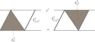
Figure 13. Family of piecewise linear functions.

The gray regions of the figure show a one parameter families of piecewise linear functions as in Figure 14, which can be converted to a one parameter family of source dependent almost complex structures and Hamiltonian vector fields as we did during the construction of $s^{1}_{c}$.

Figure 14. Family of piecewise linear functions.

We join this family of piecewise linear functions with an afine function representing $t^{1}_{c,c^{\prime}}$. Thus the third term of (16.17) corresponds to the left of Figure 13 and the second term of (16.17) corresponds to the right of Figure 13. The boundary of the two one parameter families intersect at one point which represents $t^{1}_{c,c^{\prime}}\circ t^{1}_{c^{\prime},c}\circ t^{1}_{c,c^{\prime}}$. The other ends correspond to ${\bf e}_{c}\circ t^{1}_{c,c^{\prime}}$ and $t^{1}_{c,c^{\prime}}\circ{\bf e}_{c^{\prime}}$, respectively. As (pre)natural transformations they coincide with each other, but, as piecewise linear functions or source dependent almost complex structures and Hamiltoniam vector fileds, they are different. We join them by a one parameter family of piecewise linear functions depicted by Figure 15. We call this (and similar) family as a phantom cell.

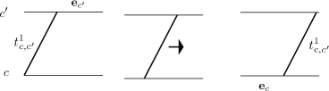
Figure 15. A phantom cell.

We thus obtain a cell decomposition of $S^{1}$ into three 1-cells which parametrize piecewise linear functions. We can find a 2-cell $\Delta^{2}$ and a family of piecewise linear functions parametrized by $\Delta^{2}$ so that on the boundary $\partial\Delta^{2}=S^{1}$ it becomes the above described $S^{1}$ parametrized family. In fact we can take $sf+(1-s)f_{0}$ where $f_{0}$ is the unique affine map so that $f_{0}(0)=0$ and $f_{0}(1)=1$ at $1$, for example. It gives a map from $\partial\Delta^{2}\times[0,1]$ to the space of piecewise linear functions. At $s=1$ the function is independent of $\partial\Delta^{2}$ factor. So it induces a map from the cone of $\partial\Delta^{2}$ to the space of piecewise linear functions.

In the same way as (16.12) and (16.13), from the family of piecewise linear functions we can obtain a $\Delta^{2}$ parametrized family of source dependent families of almost complex structures and Hamiltonian vector fields. Then for each point in the interior ${\rm Int}{\Delta^{2}}$ of $\Delta^{2}$ we obtain an equation similar to (16.14) where $R$ there is replaced by a point of ${\rm Int}{\Delta^{2}}$. At the boundary $\partial{\Delta^{2}}$ the moduli space of its solutions becomes the (fiber) products of the moduli spaces which was used to define $t^{1}_{c,c^{\prime}}$, $t^{1}_{c^{\prime},c}$, $s^{1}_{c}$, $s^{1}_{c^{\prime}}$. These moduli spaces have Kuranishi structures and CF-perturbations which are compatible with those used to define $t^{1}_{c,c^{\prime}}$, $t^{1}_{c^{\prime},c}$, $s^{1}_{c}$, $s^{1}_{c^{\prime}}$. Therefore we use those Kuranishi structures and CF-perturbations to define

(16.18) $$\phi^{2}_{c,c^{\prime};k}:CF(L,M_{0}) \otimes CF(M_{0},M_{1})$$

$$\otimes\dots\otimes CF(M_{k-1},M_{k})\to CF(\varphi(L),M_{k}).$$

This is the definition of $t^{2}_{c,c^{\prime}}$. As in the case of $s^{1}_{c}$ the moduli space we used to define $t^{2}_{c,c^{\prime}}$ has 4 types of boundaries. Three of them correspond to $\mathfrak{M}_{1}(t^{2}_{c,c^{\prime}})$. The last one is obtained from the $S^{1}=\partial\Delta^{2}$ parametrized family. Two among three 1-cells of $\partial\Delta^{2}$ give $\mathfrak{M}_{2}(t^{1}_{c,c^{\prime}},s^{1}_{c^{\prime}})$ and $\mathfrak{M}_{2}(s^{1}_{c},t^{1}_{c,c^{\prime}})$, respectively, by construction. We claim that the phantom cells do not contribute to the operation. In fact, the moduli spaces of the solutions of the equation do not change if we move on a phantom 1-cell. We can take our CF-perturbations so that this symmetry is preserved. Then the integration along the fiber is zero in the chain level. (This argument is the same as the proof of strict unitality of the degree-$0$ form $1$.) Thus we verified (16.17). The estimate of the energy loss is the same as (16.11).

To clarify the construction we will discuss one more step of the construction explicitly. We will construct $s^{2}_{c}=\{\psi^{2}_{c;k}\}$, that satisfies:

(16.19) $$\mathfrak{M}_{1}(s^{2}_{c})+\mathfrak{M}_{2}(t^{2}_{c,c^{\prime}},t^{1}_{c^{\prime},c})+\mathfrak{M}_{2}(t^{1}_{c,c^{\prime}},t^{2}_{c^{\prime},c})+\mathfrak{M}_{2}(s^{1}_{c},s^{1}_{c})=0.$$

The second, third and fourth terms of the left hand side is depicted by Figure 16 which is similar to Figure 13.

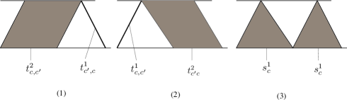
Figure 16. 2,3 and 4th terms of (16.19).

(1)(2)(3) of Figure 16 correspond 2-cells parametrizing piecewise linear functions. They are glued to give a two dimensional cell complex depicted by Figure 17 below.

Figure 17. A cell complex describing (16.19).

The 2-dimensional cell complex in Figure 17 is homeomorphic to a 2-cell and its boundary is a 1-dimensional cell complex homeomorphic to a circle and its 1-cells are phantom cells. We depict it in Figure 18 below. (The arrows in the figure show how a part of the graph moves when we move on the circle in the counter clockwise direction.)

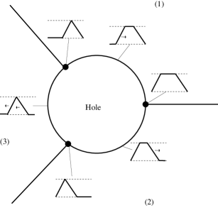
Figure 18. A circle of phantom cells.

We can fill this hole and construct a 2-cycle parametrizing a piecewise linear functions as follows.

We observe that a piecewise linear function corresponding to a point of a phantom cell has a part (a union of intervals) where the function is constant, (that is $0$ or $1$). Suppose those intervals are $[a_{1},b_{1}]$, …, $[a_{m},b_{m}]$ with $b_{i}<a_{i+1}$. (In our particular situation there are at most two such intervals. We describe this process in such a way that we can use it in more general situation also.) At time $s\in[0,1]$ we shrink the length of each such interval by the factor $(1-s)$. Namely the first interval becomes $[a_{1},b_{1}-s(b_{1}-a_{1})]$ The second interval becomes $[a_{2}-s(b_{1}-a_{1}),b_{2}-s(b_{1}-a_{1})-s(b_{2}-a_{2})]$ and etc. The exception is the case when $b_{m}=1$. In that case we do not change $b_{m}$ but change $a_{m}$ to $a_{m}-\sum_{i=1}^{m-1}s(b_{i}-a_{i})$. We move the part where the piecewise linear functions are non-constant to the left. See Figure 19.

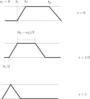
Figure 19. Fill the hole.

At $s=1$ certain parameters of a phantom cell become trivial and so the dimension of the cell complex strictly decreases. Therefore we obtain a cell complex of dimension 2 (in our case) such that its boundary is $S^{1}$. Note that the complex we use to fill the hole consists of phantom cells.

We thus obtain a 2-dimensional cell complex which parametrizes piecewise linear functions and which is a cycle.

Therefore we can find a 3-dimensional cell complex $C_{3}$ which parametrizes piecewise linear functions and whose boundary is the above 2 cycle. Thus we obtain a $C_{3}$ parametrized family of source dependent families of almost complex structures and of Hamiltonian vector fields. Then we obtain a moduli space of solutions of an equation similar to (16.14) where $R$ is replaced by an element of $C_{3}$.

We extend Kuranishi structures and CF-perturbations to these moduli spaces. Then we obtain maps $\phi^{2}_{c;k}$ as in (16.18). We thus obtained $s^{2}_{c}=\{\psi^{2}_{c;k}\}$. Using the fact that the boundary of $C_{3}$ is the union of 2-cells as in Figure 17 and phantom cells we can prove (16.19) by Stokes’ theorem ([FOOO5, Theorem 9.28]), composition formula ([FOOO5, Theorem 10.21]) and the fact that phantom cells do not contribute to the map (integration along the fiber) in the chain level.

The construction of $s^{k}_{c}$, $s^{k}_{c^{\prime}}$ and $t^{k}_{c,c^{\prime}}$, $t^{k}_{c^{\prime},c}$ for general $k$ is mostly the same as the case we already described. Let us discuss the case of $t^{k}_{c,c^{\prime}}$. The equation $t^{k}_{c,c^{\prime}}$ to satisfy is

$$\mathfrak{M}_{1}(t^{k}_{c,c^{\prime}})+\sum_{\ell=1}^{k-1}\mathfrak{M}_{2}(s^{\ell}_{c},t^{k-\ell}_{c,c^{\prime}})+\sum_{\ell=1}^{k-1}\mathfrak{M}_{2}(t^{k-\ell}_{c,c^{\prime}},s^{\ell}_{c^{\prime}})=0$$

See (12.7). By induction hypothesis, we have constructed cells of piecewise linear functions, corresponding to $s^{\ell}_{c},t^{k-\ell}_{c,c^{\prime}},t^{k-\ell}_{c,c^{\prime}},s^{\ell}_{c^{\prime}}$. We observe that those cells are glued together to give a cell complex $C_{0}$ whose boundary consists of phantom cells. This is a consequence of

$$\mathfrak{M}_{1}\left(\sum_{\ell=1}^{k-1}\mathfrak{M}_{2}(s^{\ell}_{c},t^{k-\ell}_{c,c^{\prime}})+\sum_{\ell=1}^{k-1}\mathfrak{M}_{2}(t^{k-\ell}_{c,c^{\prime}},s^{\ell}_{c^{\prime}})\right)=0$$

that follows from the induction hypothesis. Therefore in the same way as we did in Figure 19 we can shrink the length of the ‘flat’ parts of the graph of piecewise linear functions and move the other parts to the left to obtain a cell complex $D$ such that $D$ consists of phantom cells and $\partial D=\partial C_{0}$. Thus we glue $C_{0}$ and $-D$ along the boundary to obtain a cycle $C_{1}$. Therefore we obtain a cell complex $C$ parametrizing piecewise linear functions such that $\partial C=C_{1}=C_{0}\cup-D.$ Therefore using $C$ parametrized family of source dependent almost complex structures and Hamiltonian vector fields we define moduli spaces. They have Kuranishi structures and CF-perturbations which are compatible with the previously given one. We thus obtain maps which define $t^{k}_{c,c^{\prime}}$.

Here we need to remark the following. During the above construction we need to extend the CF-perturbation given at the boundary to the interior. Such a theory is developed in detail in [FOOO5, Chapter 17]. The case of a Kuranishi structure with corners is studied there. We defined a moduli space of $C$ parametrized equations. The parameter space $C$ is a cell complex and is not necessary a manifold with corners. To apply the theory of [FOOO5, Chapter 17] to our case we proceed as follows. From the construction it is obvious that the cell complex $C$ we use has a triangulation so that the triangulations of various cell complexes (used to define $s^{k}_{c},t^{k}_{c,c^{\prime}},t^{k}_{c,c^{\prime}},s^{k}_{c^{\prime}}$) are compatible at the boundary. In other words the triangulation of the boundary of the cell complex to define $s^{k}_{c}$,$t^{k}_{c,c^{\prime}}$ etc. is a subdivision of the product of those used to define $s^{\ell}_{c}$,$t^{\ell}_{c,c^{\prime}}$ etc. We remark that a simplex is a manifold with corners. So when we restrict our moduli space to the part corresponding to a simplex of the triangulation of $C$, we obtain a Kuranishi structure with corners. Therefore applying [FOOO5, Chapter 17] to each simplex inductively from those adjoining the boundary to those in the interior we can construct CF-perturbations on the parts of the moduli spaces corresponding to various simplexes so that they coincide at the overlapped part.

The last point to mention is ‘homotopy inductive limit argument’. Again we need to stop the argument at the stage when only a finite number of moduli spaces are involved. We can resolve this issue in the following way as usual. Observe that the equation we want to solve is Maurer-Cartan equation. Therefore we can define the notion of a gauge equivalence of infinite homotopy equivalences in the same way as the gauge equivalence of bounding cochains (See [FOOO1, Section 4.3]). We can also define the notion of an $(m,K)$-homotopy equivalence. Namely an $(m,K)$-homotopy equivalence assigns $t^{k}_{c,c^{\prime}}$, $s^{k}_{c}$ etc. only for $k\leq m$ and they satisfy Maurer-Cartan equation modulo $T^{K}$. The argument we have described gives such $(m,K)$-homotopy equivalence for any but finite $m$ and $K$, which we write $(\hat{t}(m,K),\hat{s}(m,K))$. Then we can show for $m<m^{\prime}$, $K<K^{\prime}$ $(\hat{t}(m,K),\hat{s}(m,K))$ is gauge equivalent to $(\hat{t}(m^{\prime},K^{\prime}),\hat{s}(m^{\prime},K^{\prime}))$ as $(m,K)$-homotopy equivalences. Then by a homological algebra we can show that $(\hat{t}(m,K),\hat{s}(m,K))$ can be extended to an $(m^{\prime},K^{\prime})$-homotopy equivalence. Therefore by an induction argument we can construct an infinite homotopy equivalence.

The proof of Theorem 12.14 is now complete. ∎

17. Completions of filtered $A_{\infty}$ categories.

In Theorem 1.3 we study Cauchy sequences of finite sets of Lagrangian submanifolds. Actually the argument of its proof works in more general case, which we discuss here.

Definition 17.1.

Let $(X,\omega)$ be a symplectic manifold which is compact or tame. We define a metric space $\overline{\mathfrak{L}}$ as follows. Its element is an equivalence class of a sequence $\{L^{n}\}$ such that

1. $L^{n}$ is a relatively spin Lagrangian submanifold of $X$. We assume $L^{n}$ is unobstructed.

2. $\sum_{n=1}^{\infty}d_{\rm Hof}(L^{n},L^{n+1})<\infty.$

Two sequences $\{L_{i}^{n}\}$, $i=1,2$ are said to be equivalent if

$$\lim_{n\to\infty}d_{\rm Hof}(L_{1}^{n},L_{2}^{n})=0.$$

We define the Hofer metric $d_{\rm Hof}([\{L^{n}_{1}\}],[\{L^{n}_{2}\}])$ between two equivalence classes by

$$d_{\rm Hof}([\{L^{n}_{1}\}],[\{L^{n}_{2}\}])=\lim_{n\to\infty}d_{\rm Hof}(L_{1}^{n},L_{2}^{n}).$$

Clearly $\overline{\mathfrak{L}}$ is a complete metric space.

Theorem 17.2.

For any separable subset $\mathbb{L}$ of $\overline{\mathfrak{L}}$ we can associate a unital completed DG-category $\mathfrak{F}(\mathbb{L})$ with the following properties.

1. The set of objects of $\mathfrak{F}(\mathbb{L})$ is an equivalence classes of pairs $([\{L^{n}\}],[(b^{n})])$ where $\{L^{n}\}$ is a Cauchy sequence converging to an element of $\mathbb{L}$ and $b^{n}$ is a sequence of bounding cochains of $L^{n}$ which has certain compatibility conditions explained during the proof.

2. $\mathfrak{F}(\mathbb{L})$ is well-defined up to equivalence.

3. If $\mathbb{L}\subseteq\mathbb{L}^{\prime}$ then $\mathfrak{F}(\mathbb{L})$ is equivalent to the full subcategory of $\mathfrak{F}(\mathbb{L}^{\prime})$.

4. If $\mathbb{L}$ is a finite set then $\mathfrak{F}(\mathbb{L})$ is equivalent to one in Theorem 1.3.

Proof.

The proof is similar to the proof of Theorem 1.3 so we will be rather sketchy. Since $\mathbb{L}$ is separable we can find a sequence of finite sets of Lagrangian submanifolds $\mathbb{L}^{n}$ with the following properties.

1. For any element $L^{\infty}$ of $\mathbb{L}$ there exists a sequence $L^{n}\in\mathbb{L}^{n}$ such that $L^{\infty}=\lim_{n\to\infty}L^{n}$.

2. For any $L^{n}\in\mathbb{L}^{n}$ there exists $L^{n+1}\in\mathbb{L}^{n+1}$ such that $d_{\rm Hof}(L^{n},L^{n+1})<\epsilon_{n}$ with $\sum\epsilon_{n}<\infty$. ($\epsilon_{n}$ is independent of $L^{n}$.)

3. The sequence $\mathbb{L}^{n}$ is strongly transversal in the sense of Definition 15.1.

The existence of $\mathbb{L}^{n}$ satisfying (a)(b) is easy to show. We can then replace $\mathbb{L}^{n}=\{L^{n}_{i}\mid i=1,\dots,m_{n}\}$ by $\mathbb{L}^{n\prime}=\{L^{n,\prime}_{i}\mid i=1,\dots,m_{n}\}$ inductively such that elements of $\mathbb{L}^{n-1}$ is transversal to elements of $\mathbb{L}^{n\prime}$ and that $d_{\rm Hof}(L^{n}_{i},L^{n,\prime}_{i})<\epsilon^{\prime}_{n}$ with $\sum\epsilon^{\prime}_{n}<\infty$. This $\mathbb{L}^{n\prime}$ has property (c) also.

We take $\epsilon_{n}$ as above and modify $\mathfrak{F}(\mathbb{L}^{n})$ to $\widehat{\mathfrak{F}}(\mathbb{L}^{n})$ as follows. For each element $[\hat{L}]$ of $\mathbb{L}$ we take and fix a sequence $\hat{L}=(L_{1},L_{2},\dots)$ such that $L_{m}\in\mathbb{L}^{m}$,

(17.1) $$d_{\rm Hof}(L^{m},L^{m+1})<2\epsilon_{m}$$

and $\hat{L}$ represents $[\hat{L}]$. Moreover we take and fix a Hamiltonian diffeomorphism $\varphi_{m}$ such that $\varphi_{m}(L_{m})=L_{m+1}$ and $d_{\rm Hof}({\rm id},\varphi_{m})<2\epsilon_{m}$. We fix such a choice for each element of $\mathbb{L}$. For $[\hat{L}],[\hat{L}^{\prime}]$ with $(L_{1},\dots,L_{m})=(L^{\prime}_{1},\dots,L^{\prime}_{m})$ we require that $\varphi_{i}=\varphi^{\prime}_{i}$ holds for $i<m$. Here $[\hat{L}],[\hat{L}^{\prime}]$ are represented by $(L_{i})_{i=1}^{\infty}$, $(L^{\prime}_{i})_{i=1}^{\infty}$ respectively and $\varphi_{i}$, $\varphi^{\prime}_{i}$ are Hamiltonian diffeomorphisms which we associate to $[\hat{L}],[\hat{L}^{\prime}]$, respectively.

The set of objects of $\widehat{\mathfrak{F}}(\mathbb{L}^{n})$ is a pair $([\hat{L}],b)$ where $[\hat{L}]$ is an element of $\mathbb{L}$ and $b$ is a bounding cochain of $L^{n}$.

The morphism module is defined by

$$CF(((L^{n},L^{n+1},\dots),b),((L^{n\prime},L^{n+1\prime},\dots),b^{\prime})):=CF((L^{n},b),(L^{n\prime},b^{\prime})),$$

where the right hand side is the Floer’s cochain module.

Using (b)(c) and (17.1) we can proceed in the same way as Step 1 of the proof of Theorem 1.3 to obtain a $\#$-unital filtered $A_{\infty}$ functor $\Phi^{n}:\widehat{\mathfrak{F}}(\mathbb{L}^{n})\to\widehat{\mathfrak{F}}(\mathbb{L}^{n+1})$ with energy loss $\epsilon_{n}$. Note that $\Phi^{n}_{\rm ob}([\hat{L}],b)=([\hat{L}],(\varphi_{n})_{*}b)$, where $\varphi_{n}$ is a Hamilton diffeomorphism which we fixed above for $[\hat{L}]$.

By property (a) the sequence $\{L^{n}\}$ represents elements of $\mathbb{L}$ and any element of $\mathbb{L}$ is represented by a certain sequence $L^{n}$. The condition $\Phi^{n}_{\rm ob}(L^{n},b^{n})=(L^{n+1},b^{n+1})$ is the condition for $b^{n}$ mentioned in (1). Thus (1) is proved.

The proof of well-defined-ness is the same as the various well-defined-ness proof of Theorem 1.3. The claims (3)(4) of Theorem 17.2 then is immediate from the construction. ∎

Remark 17.3.

There are many cases where the metric space $\overline{\mathfrak{L}}$ is not separable. An easy example is $T^{2}$. There is a continuum of Lagrangian $S^{1}$ which are geodesic with respect to the flat metric. They are unobstructed and two of such $S^{1}$ are not Hamiltonian isotopic with each other. Therefore the Hofer distance between them is infinite. So $\overline{\mathfrak{L}}$ contains uncountably many connected components. In view of the study of family Floer homologies (See [Ab, Tu, Yu].) such continuum (of pairs of Lagrangian submanifolds and their bounding cochains) becomes a set of points of a certain rigid analytic space. (Note that the topology on this set coming from rigid analytic structure is much different from the Hofer metric. The latter is finer structure in the sense that it distinguishes two Hamiltonian isotopic Lagrangian submanifolds). So we need to combine two stories somehow to obtain a filtered $A_{\infty}$ category containing ‘all’ the unobstructed Lagrangian submanifolds.

In the Fano case such as certain toric manifolds there are cases where we can take sufficiently large separable set of Lagrangian submanifolds which can play a similar role as the set of ‘all’ Lagrangian submanifolds. For example in the case $X=S^{2}$ we may take the set of all oriented great circles, which is homeomorphic to $S^{2}$.

Remark 17.4.

The difficulty to generalize the proof of Theorem 17.2 to the case when $\mathbb{L}$ is not separable, is the following. During the proof we take an $\mathbb{N}$ parametrized family of finite sets of Lagrangian submanifolds and take an inductive limit with respect to the $\mathbb{N}$ parametrized inductive system. When we consider non-separable $\mathbb{L}$ we need to consider the following situation: $\mathbb{L}_{1}$, $\mathbb{L}_{2}$, $\mathbb{L}_{3}$, $\mathbb{L}_{4}$ are finite sets of Lagrangian submanifolds and $\Phi_{ji}:\mathfrak{F}(\mathbb{L}_{i})\to\mathfrak{F}(\mathbb{L}_{j})$ for $(ji)=(21),(31),(42),(43)$ are defined. In such a situation we can still take an inductive limit if $\Phi_{42}\circ\Phi_{21}=\Phi_{43}\circ\Phi_{31}$ holds as an exact equality. We can find $\Phi_{ji}$ such that $\Phi_{42}\circ\Phi_{21}$ is homotopic (or homotopy equivalent) to $\Phi_{43}\circ\Phi_{31}$. However the exact equality is hard to achieve.

Proposition 17.5.

For a completed DG-category $\mathscr{C}$, there exists a completed DG-category $\mathscr{C}^{\prime}$ equivalent to $\mathscr{C}$ such that $\mathfrak{OB}(\mathscr{C}^{\prime})$ is complete and Hausdorff.

Proof.

The proof is mostly the same as the proof of Theorem 17.2. For $c,c^{\prime}\in\mathfrak{OB}(\mathscr{C})$ we write $c\sim c^{\prime}$ if $d_{\rm Hof,\infty}(c,c^{\prime})=0$. This is an equivalence relation. We pick up one representative from the equivalence classes to obtain $C$. We replace $\mathscr{C}$ by its full subcategory the set of whose objects is $C$. We thus may assume that $\mathfrak{OB}(\mathscr{C})$ is Hausdorff. Let $\overline{\mathfrak{OB}(\mathscr{C})}$ be the completion of $\mathfrak{OB}(\mathscr{C})$ with respect to the Hofer infinite metric. For each $\mathfrak{c}\in\overline{\mathfrak{OB}(\mathscr{C})}$ we choose a sequence of elements $\{c^{n}(\mathfrak{c})\}$ with $c^{n}(\mathfrak{c})\in\mathfrak{OB}(\mathscr{C})$ such that

(17.2) $$d_{\rm Hof,\infty}(c^{n}(\mathfrak{c}),\mathfrak{c})<\epsilon_{n}.$$

with $\epsilon_{n}\to 0$. Here $\epsilon_{n}$ is independent of $\mathfrak{c}$. In case $\mathfrak{c}=c\in\mathfrak{OB}(\mathscr{C})$ we take $c^{n}(\mathfrak{c})=c$.

We consider the completed DG-category $\mathscr{C}^{n}$ the set of whose objects is $\mathfrak{OB}(\mathscr{C})$ and for $\mathfrak{c},\mathfrak{c}^{\prime}\in\mathfrak{OB}(\mathscr{C})$ the morphism complex is defined by

$$\mathscr{C}^{n}(\mathfrak{c},\mathfrak{c}^{\prime}):=\mathscr{C}(c^{n}(\mathfrak{c}),c^{n}(\mathfrak{c}^{\prime})).$$

Structure operations are those of $\mathscr{C}$. Using (17.2) we can construct a $\#$-unital inductive system of completed DG-categories $(\{\mathscr{C}^{n}\},\{\Phi^{n}\})$. It is easy to see that the inductive limit of this inductive system is the required $\mathscr{C}^{\prime}$. ∎

18. A concluding remark: SYZ and KAM.

Let $X$ be an algebraic variety over ${\mathbb{C}}[[T]]$. We put $\Lambda_{0}^{(m)}={\mathbb{C}}[[T^{1/m}]]$ and $\Lambda^{(m)}$ be its field of fractions. We put $X^{(m)}=X\times_{{\mathbb{C}}[[T]]}\Lambda_{0}^{(m)}$ and $X^{(m)}_{\Lambda}=X\times_{{\mathbb{C}}[[T]]}\Lambda^{(m)}$. We fix a vector bundle $\mathcal{E}_{\Lambda^{(m)}}$ on $X^{(m)}_{\Lambda}$. We consider the set of all vector bundles $\mathcal{E}$ on $X^{(n)}$ such that

$$\mathcal{E}\times_{\Lambda_{0}^{(n)}}\Lambda^{(mnk)}\cong\mathcal{E}_{\Lambda^{(m)}}\times_{\Lambda^{(m)}}\Lambda^{(mnk)}$$

for some $k$. We write $\mathcal{E}\sim\mathcal{F}$ if they become isomorphic on $\Lambda_{0}^{(n^{\prime})}$ for certain $n^{\prime}$. Let $Y$ be the set of $\sim$ equivalence classes. For $[\mathcal{E}],[\mathcal{F}]\in Y$ we may choose representatives such that $\mathcal{E}$ and $\mathcal{F}$ are vector bundles on $X^{(m)}$. We define a metric $d([\mathcal{E}],[\mathcal{F}])$ so that $d([\mathcal{E}],[\mathcal{F}])<\epsilon$ if and only if there exists $n$ such that

1. There exists an isomorphism $\varphi:\mathcal{E}\times_{\Lambda^{(m)}}\Lambda^{(mn)}\to\mathcal{F}\times_{\Lambda^{(m)}}\Lambda^{(mn)}$.

2. $T^{k/mn}\varphi$ and $T^{k/mn}\varphi^{-1}$ are defined on $X\times_{\rm Spec({\mathbb{C}}[[T]])}\Lambda_{0}^{(nm)}$.

3. $k/mn<\epsilon$.

Then $(Y,d)$ becomes a metric space. Let $\overline{Y}$ be its completion. We might extend this definition to coherent sheaves or objects of its derived category. It seems likely that such a metric space is related to the space of Lagrangian submanifolds and its Hofer distance via homological mirror symmetry.

Suppose $\pi:X\to B$ is an SYG-fibration ([SYZ]). Let $f:X\to X$ be a symplectic diffeomorphism which commutes with $\pi$ and which is linear on each Lagrangian fiber. We may expect that such a symplectic diffeomorphism is obtained as a monodromy of a maximal degenerate family of Calabi-Yau manifolds ([Fu3]).

We consider its Mirror $\hat{X}$ which could be a scheme over $\Lambda_{0}^{(m)}$. Homological Mirror symmetry predicts that the fibers of $\pi:X\to B$ (at a rational point of $B$) correspond to a skyscraper sheaf $\mathcal{E}_{p}$ on $\hat{X}\times_{\Lambda_{0}^{(m)}}\Lambda^{(m)}$. For this object $\mathcal{E}_{\Lambda^{(m)}}:=\mathcal{E}_{p}$ we carry out the construction suggested above to obtain a metric space $\overline{Y_{p}}$. It is expected that $f$ via the mirror symmetry becomes an automorphism (of the derived category of coherent sheaves) given by $\mathcal{E}\mapsto\mathcal{E}\otimes\mathcal{L}$ on $\overline{Y_{p}}$ for a certain ample line bundle $\mathcal{L}$. (See [Fu6].) Note that $\mathcal{E}_{p}\otimes\mathcal{L}$ is $\mathcal{E}_{p}$ for the skyscraper sheaf $\mathcal{E}_{p}$. The sheaf on $\hat{X}\times_{\Lambda_{0}^{(m)}}\Lambda^{(m)}$ which corresponds to the fiber is a fixed point of this automorphism.

Now we take $f_{\epsilon}$ which is sufficiently close to $f$. The KAM theorem seems to say that the Mirror $\hat{f}_{\epsilon}$ to $f_{\epsilon}$ (that is an isometry and $x\mapsto d(x,f_{\epsilon}(x))$ is bounded) has a fixed point on $Y_{p}$ for $p$ in a subset of almost full measure.

The space $\overline{Y_{p}}$ seems to be closely related to a space appearing in rigid analytic geometry. It might be possible to expect that there is a certain fixed point theorem which implies the existence of a fixed point of $\hat{f}_{\epsilon}$ on $\overline{Y_{p}}$.

It would be very interesting if one can relate such a fixed point theorem to the KAM theory and also relate the existence of KAM tori with the existence of a fixed point of $\hat{f}_{\epsilon}$ on $Y_{p}$.

References

- [Ab] M. Abouzaid, Family Floer cohomology and mirror symmetry, Proceedings of the International Congress of Mathematicians—Seoul 2014. Vol. II, 813–836, Kyung Moon Sa, Seoul, 2014.
- [AFOOO] M. Abouzaid, K. Fukaya, Y.-G. Oh, H. Ohta and K. Ono, Quantum cohomology and split generation in Lagrangian Floer theory, in preparation.
- [Ad] J.F. Adams, On the Cobar Construction, Proceedings of the National Academy of Sciences of the United States of America 42-7 (1956), 409–412.
- [AJ] M. Akaho and D. Joyce, Immersed Lagrangian Floer theory, J. Differential Geometry 86 (2010) 381-500.
- [Ba] A. Barannikov, The framed Morse complex and its invariants Singularities and bifurcations, Adv. Soviet. Math. 21 Amer. Math. Soc., Providence, (1994) 93–115.
- [BCS] P. Biran, O Cornea and E. Shelvkin, Lagrangian Shadows and triangulated Categories. arXiv:1806.06630.
- [Ch1] Y. Chekanov, Lagrangian intersections, symplectic energy, and areas of holomorphic curves, Duke Math. J. 95 (1998), no. 1, 213–226.
- [Ch2] Y. Chekanov, Invariant Finsler metrics on the space of Lagrangian embeddings, Math. Z., 234 (2000) 605–619.
- [Fu1] K. Fukaya, Hausdorff convergence of Riemannian manifolds and its applications, in “Recent Topics in Differential and Analytic Geometry” ed. by T. Ochiai, Advanced Studies in Pure Mathematics, Kinokuniya, Tokyo (1990), 143 – 238.
- [Fu2] K. Fukaya, Floer homology and mirror symmetry II, Minimal Surfaces, Geometric Analysis and Symplectic Geometry (Baltimore, MD, 1999), Adv. Stud. Pure Math. 34 (2002), 31–127.
- [Fu3] K. Fukaya, Galois symmetry on Floer cohomology, Turkish J. Math. 27 (2003), 11–32.
- [Fu4] K. Fukaya, Cyclic symmetry and adic convergence in Lagrangian Floer theory, Kyoto J. Math. 50 (2010), no. 3, 521–590.
- [Fu5] K. Fukaya, Unobstructed immersed Lagrangian correspondences and filtered functors, ArXiv 1706.02131v2.
- [Fu6] K. Fukaya, Lecture at Kyoto University 2021 January; SYZ and KAM, A note is on http://scgp.stonybrook.edu/people/faculty/bios/kenji-fukaya.
- [FOOO1] K. Fukaya, Y.-G. Oh, H. Ohta and K. Ono, Lagrangian intersection Floer theory-anomaly and obstruction, Part I, AMS/IP Studies in Advanced Math. vol. 46.1, International Press/ Amer. Math. Soc. (2009). MR2553465.
- [FOOO2] K. Fukaya, Y.-G. Oh, H. Ohta and K. Ono, Lagrangian intersection Floer theory-anomaly and obstruction, Part II, AMS/IP Studies in Advanced Math. vol. 46.2, International Press/ Amer. Math. Soc. (2009). MR2548482.
- [FOOO3] K. Fukaya, Y.-G. Oh, H. Ohta and K. Ono, Displacement of polydisks and Lagrangian Floer theory, J. Symplectic Geom. 11 (2013), no 2, 231–268
- [FOOO4] K. Fukaya, Y.-G. Oh, H. Ohta and K. Ono, Construction of Kuranishi structures on the moduli spaces of pseudo holomorphic disks: I, Surveys in Differential Geometry 22 (2018) 133-190, arXiv:1710.01459.
- [FOOO5] K. Fukaya, Y.-G. Oh, H. Ohta and K. Ono, Kuranishi structures and Virtual fundamental chains, (2020) Springe Monograph in Mathematics, xv+638, Springer, Singapore ISBN 978-981-15-5562-6.
- [FOOO6] K. Fukaya, Y.-G. Oh, H. Ohta and K. Ono, Construction of Kuranishi structures on the moduli spaces of pseudo-holomorphic disks: II, arXiv:1808.06106.
- [GLP] M. Gromov, J. Lafontaine and P. Pansu, Structure métrique pour variétés riemanniennes, Cedic/Fernand Nathan, Paris 1981
- [Ho] H. Hofer, On the topological properties of symplectic maps, Proc. Royal Soc. Edinburgh 115 (1990), 25–38.
- [Ka] T.V. Kadeišivili, The algebraic structure in the homology of an -algebra, Soobshch. Akad. Nauk Gruzin. SSR 108 (1982) 249–252. (in Russian).
- [Ke] B. Keller, A-infinity algebras, modules and functor categories, arXiv:math/0510508.
- [Le] K. Lefèvre-Hasegawa, Sur les catégories, Thése Doctorat Universite Paris 7 (2003).
- [Os] Y. Ostrover, A comparison Hofer’s metric on Hamiltonian diffeomorphisms and Lagrangian submanmifolds, Commun. Contemp. Math. 5 (2003) 803–311.
- [PS] L. Polterovich and E. Shelukhin, Autonomous Hamiltonian flows, Hofer’s geometry, and persistent modules, Selecta Math. 22 (2016) 227–296.
- [PRSZ] L. Polterovich, D. Rosen, K. Samvelyan and J. Zhang, Persistence in Geometry and Analysis , Amer. Math. Soc., Providence, (2020).
- [RSV] F. Le Roux, S. Seyfaddini and C. Viterbo, Barcodes and area-preserving homeomorphisms , ArXive:1810.03139.
- [Se] P. Seidel, Fukaya categories and Picard-Lefschetz theory, ETH Lecture Notes series of the European Math. Soc., 2008.
- [SYZ] A Strominger, S-T Yau, and E Zaslow. Mirror symmetry is T-duality, Nuclear Physics. B, 479(1- 2):243–259, 1996.
- [Tu] J. Tu On the reconstruction problem in mirror symmetry, Advances in Mathematics, 256:449–478, 2014.
- [Us] M. Usher, Boundary depth in Floer theory and its applications to Hamiltonian dynamics and coisotropic submanifolds, Israel J. Math. 184 (2011), 1–57.
- [Yu] H. Yuan, Family Floer program and non-archimedean SYZ mirror construction, arXiv:2003.06106.