Improving Bridge estimators via $f$-GAN

Abstract

Bridge sampling is a powerful Monte Carlo method for estimating ratios of normalizing constants. Various methods have been introduced to improve its efficiency. These methods aim to increase the overlap between the densities by applying appropriate transformations to them without changing their normalizing constants. In this paper, we first give a new estimator of the asymptotic relative mean square error (RMSE) of the optimal Bridge estimator by equivalently estimating an $f$-divergence between the two densities. We then utilize this framework and propose $f$-GAN-Bridge estimator ($f$-GB) based on a bijective transformation that maps one density to the other and minimizes the asymptotic RMSE of the optimal Bridge estimator with respect to the densities. This transformation is chosen by minimizing a specific $f$-divergence between the densities. We show $f$-GB is optimal in the sense that within any given set of candidate transformations, the $f$-GB estimator can asymptotically achieve an RMSE lower than or equal to that achieved by Bridge estimators based on any other transformed densities. Numerical experiments show that $f$-GB outperforms existing methods in simulated and real-world examples. In addition, we discuss how Bridge estimators naturally arise from the problem of $f$-divergence estimation.

Keywords: Monte Carlo estimation, Normalizing constants, Bayes factor, $f$-divergence, Generative adversarial network, Normalizing flow

1 Introduction

Estimating the normalizing constant of an unnormalized probability density, or the ratio of normalizing constants between two unnormalized densities is a challenging and important task. In Bayesian inference, such problems are closely related to estimating the marginal likelihood of a model or the Bayes factor between two competing models, and can arise from fields such as econometrics (Geweke,, 1999), astronomy (Bridges et al.,, 2009), phylogenetics (Fourment et al.,, 2020), etc. Monte Carlo methods such as Bridge sampling (Bennett,, 1976; Meng and Wong,, 1996), path sampling (Gelman and Meng,, 1998), reverse logistic regression (Geyer,, 1994), nested sampling Skilling et al., (2006) and reverse Annealed Importance Sampling (Burda et al.,, 2015) have been proposed to address this problem. See Friel and Wyse, (2012) for an overview of some popular algorithms. Fourment et al., (2020) also compare the empirical performance of 19 algorithms for estimating normalizing constants in the context of phylogenetics.

Bridge sampling (Bennett,, 1976; Meng and Wong,, 1996) is a powerful, easy-to-implement Monte Carlo method for estimating the ratio of normalizing constants. Let $\tilde{q}_{i}(\omega),\omega\in\Omega_{i},\ i=1,2$ be two unnormalized probability densities with respect to a common measure $\mu$. Let $q_{i}(\omega)=\tilde{q}_{i}(\omega)/Z_{i}$ be the corresponding normalized density, where $Z_{i}$ is the normalizing constant. Bridge sampling estimates $r=Z_{1}/Z_{2}$ using samples from $q_{1},q_{2}$ and the unnormalized density functions $\tilde{q}_{1},\tilde{q}_{2}$. Meng and Schilling, (2002) point out that Bridge sampling is equally useful for estimating a single normalizing constant. The relative mean square error (RMSE) of a Bridge estimator depends on the overlap or “distance” between $q_{1},q_{2}$. The overlap can be quantified by some divergence between them. When $q_{1},q_{2}$ share little overlap, the corresponding Bridge estimator has large RMSE and therefore is unreliable. In order to improve the efficiency of Bridge estimators, various methods such as Warp Bridge sampling (Meng and Schilling,, 2002), Warp-U Bridge sampling (Wang et al.,, 2020) and Gaussianized Bridge sampling (Jia and Seljak,, 2020) have been introduced. These methods first apply transformations $T_{i}$ to $q_{i}$ in a tractable way without changing the normalizing constant $Z_{i}$ for $i=1,2$, then compute Bridge estimators based on the transformed densities $q_{i}^{(T)}$ and the corresponding samples for $i=1,2$. If $q_{1}^{(T)},q_{2}^{(T)}$ have greater overlap than the original ones, then the resulting Bridge estimator of $r$ based on $q_{1}^{(T)},q_{2}^{(T)}$ would have a lower RMSE.

In this paper, we first demonstrate the connection between Bridge estimators and $f$-divergence (Ali and Silvey,, 1966). We show that one can estimate the asymptotic RMSE of the optimal Bridge estimator by equivalently estimating a specific $f$-divergence between $q_{1},q_{2}$. Nguyen et al., (2010) propose a general variational framework for $f$-divergence estimation. We apply this framework to our problem and obtain a new estimator of the asymptotic RMSE of the optimal Bridge estimator using the unnormalized densities $\tilde{q}_{1},\tilde{q}_{2}$ and the corresponding samples. We also find a connection between Bridge estimators and the variational lower bound of $f$-divergence given by Nguyen et al., (2010). In particular, we show that the problem of estimating an $f$-divergence between $q_{1},q_{2}$ using this variational framework naturally leads to a Bridge estimator of $r=Z_{1}/Z_{2}$. Kong et al., (2003) observe that the optimal Bridge estimator is a maximum likelihood estimator under a semi-parametric formulation. We use this $f$-divergence estimation framework to extend this observation and show that many special cases of Bridge estimators such as the geometric Bridge estimator can also be interpreted as maximizers of some objective functions that are related to the $f$-divergence between $q_{1},q_{2}$. This formulation also connects Bridge estimators and density ratio estimation problems: Since we can evaluate the unnormalized densities $\tilde{q}_{1},\tilde{q}_{2}$, we know the true density ratio up to a multiplicative constant $r=Z_{1}/Z_{2}$. Hence estimating $r$ can be viewed as a problem of estimating the density ratio between $q_{1},q_{2}$. A similar idea has been explored in e.g. Noise Contrastive Estimation (Gutmann and Hyvärinen,, 2010), where the authors treat the unknown normalizing constant as a model parameter, and cast the estimation problem as a classification problem. Similar ideas have also been discussed in e.g. Geyer, (1994) and Uehara et al., (2016).

We then utilize the connection between the asymptotic RMSE of the optimal Bridge estimator and a specific $f$-divergence between $q_{1},q_{2}$, and propose $f$-GAN-Bridge estimator ($f$-GB), which improves the efficiency of the optimal Bridge estimator of $r$ by directly minimizing the first order approximation of its asymptotic RMSE with respect to the densities using an $f$-GAN. $f$-GAN (Nowozin et al.,, 2016) is a class of generative model that aims to approximate the target distribution by minimizing an $f$-divergence between the generative model and the target. Let $\mathcal{T}$ be a collection of transformations $T$ such that $\tilde{q}_{1}^{(T)}$, the transformed unnormalized density of $q_{1}$ is computationally tractable and have the same normalizing constant $Z_{1}$ as the original $\tilde{q}_{1}$. The $f$-GAN-Bridge estimator is obtained using a two-step procedure: We first use the $f$-GAN framework to find the transformation $T^{*}$ that minimizes a specific $f$-divergence between $q_{1}^{(T)}$ and $q_{2}$ with respect to $T\in\mathcal{T}$. Once $T^{*}$ and $q_{1}^{(T^{*})}$ are chosen, we then compute the optimal Bridge estimator of $r$ based on $q_{1}^{(T^{*})}$ and $q_{2}$ as the $f$-GAN-Bridge estimator. We show $T^{*}$ asymptotically minimizes the first order approximation of the asymptotic RMSE of the optimal Bridge estimator based on $q_{1}^{(T)}$ and $q_{2}$ with respect to $T$. In contrast, existing methods such as Warp Bridge sampling (Meng and Schilling,, 2002; Wang et al.,, 2020) and Gaussianized Bridge sampling (Jia and Seljak,, 2020) do not offer such theoretical guarantee. The transformed $q_{1}^{(T)}$ can be parameterized in any way as long as it is computationally tractable and preserves the normalizing constant $Z_{1}$. In this paper, we parameterize $q_{1}^{(T)}$ as a Normalizing flow (Rezende and Mohamed,, 2015; Dinh et al.,, 2016) with base density $q_{1}$ because of its flexibility.

1.1 Summary of our contributions

The main contribution of our paper is that we give a computational framework to improve the optimal Bridge estimator by minimizing the first order approximation of its asymptotic RMSE with respect to the densities. We also give a new estimator of the asymptotic RMSE of the optimal Bridge estimator using the variational framework proposed by Nguyen et al., (2010). This formulation allows us to cast the estimation problem as a 1-d optimization problem. We find the $f$-GAN-Bridge estimator outperforms existing methods significantly in both simulated and real-world examples. Numerical experiments show that the proposed method provides not only a reliable estimate of $r$, but also an accurate estimate of its RMSE. In addition, we also find a connection between Bridge estimators and the problem of $f$-divergence estimation, which allows us to view Bridge estimators from a different perspective.

This paper is structured as follows: In Section 2, we briefly review Bridge sampling and existing improvement strategies. In Section 3, we give a new estimator of the asymptotic RMSE of the optimal Bridge estimator using the variational framework for $f$-divergence estimation (Nguyen et al.,, 2010). We also demonstrate the connection between Bridge estimators and the problem of $f$-divergence estimation. In Section 4, we introduce the $f$-GAN-Bridge estimator and give implementation details. We give both simulated and real-world examples in Section 5, 6. Section 7 concludes the paper with a discussion. A Python implementation of the proposed method alongside with examples can be found on Github. A Python implementation of the proposed method alongside with examples can be found in https://github.com/hwxing3259/Bridge_sampling_and_fGAN.

2 Bridge sampling and related works

Let $Q_{1},Q_{2}$ be two probability distributions of interest. Let $q_{i}(\omega),\omega\in\Omega_{i},i=1,2$ be the densities of $Q_{1},Q_{2}$ with respect to a common measure $\mu$ defined on $\Omega_{1}\cup\Omega_{2}$, where $\Omega_{1}$ and $\Omega_{2}$ are the corresponding supports. We use $\tilde{q}_{i}(\omega),i=1,2$ to denote the unnormalized densities and $Z_{i},i=1,2$ to denote the corresponding normalizing constants, i.e. $q_{i}(\omega)=\tilde{q}_{i}(\omega)/Z_{i}$ for $i=1,2$. Suppose we have samples from $q_{1},q_{2}$, but we are only able to evaluate the unnormalized densities $\tilde{q}_{i}(\omega),i=1,2$. Our goal is to estimate the ratio of normalizing constants $r=Z_{1}/Z_{2}$ using only $\tilde{q}_{i}(\omega),i=1,2$ and samples from the two distributions. Bridge sampling (Bennett,, 1976; Meng and Wong,, 1996) is a powerful method for this task.

Definition 2.1 (Bridge estimator).

Suppose $\mu(\Omega_{1}\cap\Omega_{2})>0$ and $\alpha:\Omega_{1}\cap\Omega_{2}\to\mathbb{R}$ satisfies $0<\left|\int_{\Omega_{1}\cap\Omega_{2}}\alpha(\omega)q_{1}(\omega)q_{2}(\omega)d\mu(\omega)\right|<\infty$. Given samples $\{\omega_{ij}\}_{j=1}^{n_{i}}\sim q_{i}$ for $i=1,2$, the Bridge estimator $\hat{r}_{\alpha}$ of $r=Z_{1}/Z_{2}$ is defined as

$$\hat{r}_{\alpha}=\frac{{n_{2}}^{-1}\sum_{j=1}^{n_{2}}\alpha(\omega_{2j})\tilde{q}_{1}(\omega_{2j})}{{n_{1}}^{-1}\sum_{j=1}^{n_{1}}\alpha(\omega_{1j})\tilde{q}_{2}(\omega_{1j})}$$ (1)

The choice of free function $\alpha$ directly affects the quality of $\hat{r}_{\alpha}$, which is quantified by the relative mean square error (RMSE) $E(\hat{r}_{\alpha}-r)^{2}/r^{2}$. Let $n=n_{1}+n_{2}$ and $s_{i}=n_{i}/n$ for $i=1,2$. Let $RE^{2}(\hat{r}_{\alpha})$ denote the asymptotic RMSE of $\hat{r}_{\alpha}$ as $n_{1},n_{2}\rightarrow\infty$. Under the assumption that the samples from $q_{1},q_{2}$ are i.i.d., Meng and Wong, (1996) show the optimal $\alpha$ which minimizes the first order approximation of $RE^{2}(\hat{r}_{\alpha})$ takes the form

$$\alpha_{opt}(\omega)\propto\frac{1}{s_{1}\tilde{q}_{1}(\omega)+s_{2}\tilde{q}_{2}(\omega)r},\quad\omega\in\Omega_{1}\cap\Omega_{2}$$ (2)

The resulting $RE^{2}(\hat{r}_{\alpha_{opt}})$ with the optimal free function $\alpha_{opt}$ is

$$RE^{2}(\hat{r}_{\alpha_{opt}})=\frac{1}{ns_{1}s_{2}}\left[\left(\int_{\Omega_{1}\cap\Omega_{2}}\frac{q_{1}(\omega)q_{2}(\omega)}{s_{1}q_{1}(\omega)+s_{2}q_{2}(\omega)}d\mu(\omega)\right)^{-1}-1\right]+o\left(\frac{1}{n}\right).$$ (3)

Note that the optimal $\alpha_{opt}$ is not directly usable as it depends on the unknown quantity $r$ we would like to estimate in the first place. To resolve this problem, Meng and Wong, (1996) give an iterative procedure

$$\hat{r}^{(t+1)}=\frac{n_{2}^{-1}\sum_{j=1}^{n_{2}}\tilde{q}_{1}(\omega_{2j})/(s_{1}\tilde{q}_{1}(\omega_{2j})+s_{2}\tilde{q}_{2}(\omega_{2j})\hat{r}^{(t)})}{n_{1}^{-1}\sum_{j=1}^{n_{1}}\tilde{q}_{2}(\omega_{1j})/(s_{1}\tilde{q}_{1}(\omega_{1j})+s_{2}\tilde{q}_{2}(\omega_{1j})\hat{r}^{(t)})},\quad t=0,1,2,...$$ (4)

The authors show that for any initial value $\hat{r}^{(0)}$, $\hat{r}^{(t)}$ is a consistent estimator of $r$ for all $t\geq 1$, and the sequence $\{\hat{r}^{(t)}\},\ t=0,1,2,...$ converges to the unique limit $\hat{r}_{opt}$. Let $MSE(\log\hat{r}_{opt})$ denote the asymptotic mean square error of $\log\hat{r}_{opt}$.

Under the i.i.d. assumption, the authors also show $RE^{2}(\hat{r}_{opt})$ and $MSE(\log\hat{r}_{opt})$ are asymptotically equivalent to $RE^{2}(\hat{r}_{\alpha_{opt}})$ in (3) up to the first order (i.e. they have the same leading term). Note that $\hat{r}_{opt}$ can be found numerically while $\hat{r}_{\alpha_{opt}}$ is not directly computable. We will focus on the asymptotically optimal Bridge estimator $\hat{r}_{opt}$ for the rest of the paper.

2.1 Improving Bridge estimators via transformations

From (3) and the fact that $RE^{2}(\hat{r}_{opt})$ and $RE^{2}(\hat{r}_{\alpha_{opt}})$ are asymptotically equivalent, we see $RE^{2}(\hat{r}_{opt})$ depends on the overlap between $q_{1}$ and $q_{2}$. Even when $\Omega_{1}=\Omega_{2}$, if $q_{1}$ and $q_{2}$ put their probability mass on very different regions, the integral in (3) would be close to 0, leading to large RMSE and unreliable estimators. In order to improve the performance of $\hat{r}_{opt}$, one may apply transformations to $q_{1},q_{2}$ (and to the corresponding samples) to increase their overlap while keeping the transformed unnormalized densities computationally tractable and the normalizing constants unchanged. We assume that we are dealing with unconstrained, continuous random variables with a common support, i.e. $\Omega_{1}=\Omega_{2}=\mathbb{R}^{d}$. When the supports $\Omega_{1},\Omega_{2}$ are constrained or different from each other, we can usually match them by applying simple invertible transformations to $q_{1}$, $q_{2}$. When $\Omega_{1}$,$\Omega_{2}$ have different dimensions, Chen and Shao, (1997) suggest matching the dimensions of $q_{1},q_{2}$ by augmenting the lower dimensional distribution using some completely known random variables (See Appendix 9 for details).

Voter, (1985) gives a method to increase the overlap in the context of free energy estimation by shifting the samples from one distribution to the other and matching their modes. Meng and Schilling, (2002) extends this idea and consider more general mappings. Let $T_{i}:\mathbb{R}^{d}\to\mathbb{R}^{d}$, $i=1,2$ be two smooth and invertible transformations that aim to bring $q_{1},q_{2}$ “closer”. For $\omega_{i}\sim q_{i}$, define $\omega_{i}^{(T)}=T_{i}(\omega_{i})$, $\ i=1,2$. Then for $i=1,2$, the distribution of the transformed sample $\omega_{i}^{(T)}$ has density

$$q_{i}^{(T)}(\omega_{i}^{(T)}) =\tilde{q}_{i}(T_{i}^{-1}(\omega_{i}^{(T)}))\left|\det J_{i}(\omega_{i}^{(T)})\right|/Z_{i}$$ (5)

$$\equiv\tilde{q}_{i}^{(T)}(\omega_{i}^{(T)})/Z_{i},\quad i=1,2$$ (6)

where $\tilde{q}_{i}^{(T)}$ is the unnormalized version of $q_{i}^{(T)}$, $T_{i}^{-1}$ is the inverse transformation of $T_{i}$ and $J_{i}(\omega)$ is its Jacobian. One can then apply (1) to the transformed samples and the corresponding unnormalized densities $\tilde{q}_{1}^{(T)},\tilde{q}_{2}^{(T)}$, and obtain a Bridge estimator

$$\hat{r}^{(T)}_{\alpha}=\frac{n_{2}^{-1}\sum_{j=1}^{n_{2}}\tilde{q}_{1}^{(T)}(T_{2}(\omega_{2j}))\alpha(T_{2}(\omega_{2j}))}{n_{1}^{-1}\sum_{j=1}^{n_{1}}\tilde{q}_{2}^{(T)}(T_{1}(\omega_{1j}))\alpha(T_{1}(\omega_{1j}))}$$ (7)

without the need to sample from $\tilde{q}_{1}^{(T)}$ or $\tilde{q}_{2}^{(T)}$ separately. Let $\hat{r}_{opt}^{(T)}$ denote the asymptotically optimal Bridge estimator based on the transformed densities. We stress that the superscript of $\hat{r}^{(t)}$ in (4) indicates the number of iterations, while the superscript in $\hat{r}_{opt}^{(T)}$ means it is based on the transformed densities. If the transformed $q_{1}^{(T)},q_{2}^{(T)}$ have a greater overlap than the original $q_{1},q_{2}$, then $\hat{r}^{(T)}_{opt}$ should be a more reliable estimator of $r$ with a lower RMSE. Meng and Schilling, (2002) further extend this idea and propose the Warp transformation, which aims to increase the overlap by centering, scaling and symmetrizing the two densities $q_{1},q_{2}$. One limitation of the Warp transformation is that it does not work well for multimodal distributions. Wang et al., (2020) propose the Warp-U transformation to address this problem. The key idea of the Warp-U transformation is to first approximate $q_{i}$ by a mixture of Normal or $t$ distributions, then construct a coupling between them which allows us to map $q_{i}$ into a unimodal density in the same way as mapping the mixture back to a single standard Normal or $t$ distribution.

An alternative to the Warp transformation (Meng and Schilling,, 2002) is a Normalizing flow. A Normalizing flow (NF) (Rezende and Mohamed,, 2015; Dinh et al.,, 2016; Papamakarios et al.,, 2017) parameterizes a continuous probability distribution by mapping a simple base distribution (e.g. standard Normal) to the more complex target using a bijective transformation $T$, which is parameterized as a composition of a series of smooth and invertible mappings $f_{1},...,f_{K}$ with easy-to-compute Jacobians. This $T$ is applied to the “base” random variable $z_{0}\sim p_{0}$, where $z_{0}\in\mathbb{R}^{d}$ and $p_{0}$ is the known base density. Let

$$z_{k}=f_{k}\circ f_{k-1}\circ...\circ f_{1}(z_{0}),\quad k=1,...,K$$ (8)

Since the transformation $T$ is smooth and invertible, by applying change of variable repeatedly, the final output $z_{K}$ has density

$$p_{K}(z_{K})=p_{0}(z_{0})\prod_{k=1}^{K}\left|\det J_{k}(z_{k-1})\right|^{-1}$$ (9)

where $J_{k}$ is the Jacobian of the mapping $f_{k}$. The final density $p_{K}$ can be used to approximate target distributions with complex structure, and one can sample from $p_{K}$ easily by applying $T=f_{K}\circ f_{K-1}\circ...\circ f_{1}$ to $z_{0}\sim p_{0}$. In order to evaluate $p_{K}$ efficiently, we are restricted to transformations $f_{k}$ whose $\det J_{k}(z)$ is easy to compute. For example, Real-NVP (Dinh et al.,, 2016) uses the following transformation: For $m\in\mathbb{N}$ such that $1<m<d$, let $z_{1:m}$ be the first $m$ entries of $z\in\mathbb{R}^{d}$, let $\times$ be element-wise multiplication and let $\mu_{k},\sigma_{k}:\mathbb{R}^{m}\to\mathbb{R}^{d-m}$ be two mappings (usually parameterized by neural nets). The smooth and invertible transformation $y=f_{k}(z)$ for each step $k$ in Real-NVP is defined as

$$y_{1:m}=z_{1:m},\quad y_{m+1:d}=\mu_{k}(z_{1:m})+\sigma_{k}(z_{1:m})\times z_{m+1:d}$$ (10)

This means $f_{k}$ keeps the first $m$ entries of input $z$, while shifting and scaling the remaining ones. The Jacobian $J_{k}$ of $f_{k}$ is lower triangular, hence $\det J_{k}(z)=\prod_{i=1}^{d-m}\sigma_{ik}(z_{1:m})$, where $\sigma_{ik}(z_{1:m})$ is the $i$th entry of $\sigma_{k}(z_{1:m})$. Each transformation $f_{k}$ is also called a coupling layer. When composing a series of coupling layers $f_{1},...,f_{K}$, the authors also swap the ordering of indices in (10) so that the dimensions that are kept unchanged in one step $k$ are to be scaled and shifted in the next step. Jia and Seljak, (2020) utilize the idea of transforming $q_{i}$ using a Normalizing flow, and propose Gaussianzed Bridge sampling (GBS) for estimating a single normalizing constant. The authors set $q_{1}$ to be a completely known density, e.g. standard multivariate Normal, and aim to approximate the target $q_{2}$ using a Normalizing flow with base density $q_{1}$. The transformed density $q_{1}^{(T)}$ is estimated by matching the marginal distributions between $q_{1}^{(T)}$ and $q_{2}$. Once $q_{1}^{(T)}$ is chosen, the authors use (7) and the iterative procedure (4) to form the asymptotically optimal Bridge estimator of $Z_{2}$ based on the transformed $q_{1}^{(T)}$ and the original $q_{2}$.

The idea of increasing overlap via transformations is also applicable to discrete random variables. For example, Meng and Schilling, (2002) suggest using swapping and permutation to increase the overlap between two discrete distributions. Tran et al., (2019) also give Normalizing flow models applicable to discrete random variables based on modulo operations. We give a toy example of increasing the overlap between two discrete distributions using Normalizing flows in Appendix 14. In the later sections, we will extend the idea of increasing overlap via transformations, and propose a new strategy to improve $\hat{r}^{(T)}_{opt}$ by directly minimizing the first order approximation of $RE^{2}(\hat{r}^{(T)}_{opt})$ with respect to the transformed densities.

3 Bridge estimators and $f$-divergence estimation

Frühwirth-Schnatter, (2004) gives an MC estimator of $RE^{2}(\hat{r}_{opt})$. In this section, we introduce an alternative estimator of $RE^{2}(\hat{r}_{opt})$ and $MSE(\log\hat{r}_{opt})$ by equivalently estimating an $f$-divergence between $q_{1},q_{2}$. This formulation allows us to utilize the variational lower bound of $f$-divergence given by Nguyen et al., (2010), and cast the problem of estimating $RE^{2}(\hat{r}_{opt})$ as a 1-d optimization problem. In the later section, we will also show how to use this new estimator to improve the efficiency of $\hat{r}^{(T)}_{opt}$. In addition, we find that estimating different choices of $f$ divergences under the variational framework proposed by Nguyen et al., (2010) naturally leads to Bridge estimators of $r$ with different choices of free function $\alpha(\omega)$.

3.1 Estimating $RE^{2}(\hat{r}_{opt})$ via $f$-divergence estimation

$f$-divergence (Ali and Silvey,, 1966) is a broad class of divergences between two probability distributions. By choosing $f$ accordingly, one can recover common divergences between probability distributions such as KL divergence $KL(q_{1},q_{2})$, Squared Hellinger distance $H^{2}(q_{1},q_{2})$ and total variation distance $d_{TV}(q_{1},q_{2})$.

Definition 3.1 ($f$-divergence).

Suppose the two probability distributions $Q_{1},Q_{2}$ have absolutely continuous density functions $q_{1}$ and $q_{2}$ with respect to a base measure $\mu$ on a common support $\Omega$. Let the generator function $f:\mathbb{R}^{+}\rightarrow\mathbb{R}$ be a convex and lower semi-continuous function satisfying $f(1)=0$. The $f$-divergence $D_{f}(q_{1},q_{2})$ defined by $f$ takes the form

$$D_{f}(q_{1},q_{2})=\int_{\Omega}f\left(\frac{q_{1}(\omega)}{q_{2}(\omega)}\right)q_{2}(\omega)d\mu(\omega)$$ (11)

Unless otherwise stated, we assume $\Omega=\mathbb{R}^{d}$ where $d\in\mathbb{N}$ i.e. both $q_{1}$ and $q_{2}$ are defined on $\mathbb{R}^{d}$. If the densities $q_{1},q_{2}$ have different or disjoint supports $\Omega_{1}$, $\Omega_{2}$, then we apply appropriate transformations and augmentations discussed in the previous sections to ensure that the transformed and augmented densities (if necessary) are defined on the common support $\Omega=\mathbb{R}^{d}$. In this paper, we focus on a particular choice of $f$-divergence that is closely related to $RE^{2}(\hat{r}_{opt})$ in (3).

Definition 3.2.

(Weighted harmonic divergence) Let $q_{1},q_{2}$ be continuous densities with respect to a base measure $\mu$ on the common support $\Omega$. The weighted harmonic divergence is defined as

$$H_{\pi}(q_{1},q_{2})=1-\int_{\Omega}\left(\pi q_{1}^{-1}(\omega)+(1-\pi)q_{2}^{-1}(\omega)\right)^{-1}d\mu(\omega)$$ (12)

where $\pi\in(0,1)$ is the weight parameter.

Wang et al., (2020) observe that the weighted harmonic divergence $H_{\pi}(q_{1},q_{2})$ is an $f$-divergence with generator $f(u)=1-\frac{u}{\pi+(1-\pi)u}$, and $RE^{2}(\hat{r}_{opt})$ can be rearranged as

$$RE^{2}(\hat{r}_{opt})=(s_{1}s_{2}n)^{-1}\left((1-H_{s_{2}}(q_{1},q_{2}))^{-1}-1\right)+o\left(\frac{1}{n}\right).$$ (13)

The same statement also holds for $MSE(\log\hat{r}_{opt})$ since $MSE(\log\hat{r}_{opt})$ is asymptotically equivalent to $RE^{2}(\hat{r}_{opt})$ (Meng and Wong,, 1996). This means if we have an estimator of $H_{s_{2}}(q_{1},q_{2})$, then we can plug it into the leading term of the right hand side of (13) and obtain an estimator of the first order approximation of $RE^{2}(\hat{r}_{opt})$ and $MSE(\log\hat{r}_{opt})$. Before we give the estimator of $H_{s_{2}}(q_{1},q_{2})$, we first introduce the variational framework for $f$-divergence estimation proposed by Nguyen et al., (2010). Every convex, lower semi-continuous function $f:\mathbb{R}^{+}\rightarrow\mathbb{R}$ has a convex conjugate $f^{*}$ which is defined as follows,

Definition 3.3.

(Convex conjugate) Let $f:\mathbb{R}^{+}\rightarrow\mathbb{R}$ be a convex and lower semi-continuous function. The convex conjugate of $f$ is defined as

$$f^{*}(t)=\sup_{u\in\mathbb{R}^{+}}\{ut-f(u)\}$$ (14)

Nguyen et al., (2010) show that any $f$-divergence $D_{f}(q_{1},q_{2})$ satisfies

$$D_{f}(q_{1},q_{2}) \geq\sup_{V\in\mathcal{V}}\Big{(}E_{q_{1}}[V(\omega)]-E_{q_{2}}[f^{*}(V(\omega))]\Big{)},$$ (15)

where $\mathcal{V}$ is an arbitrary class of functions $V:\Omega\to\mathbb{R}$, and $f^{*}(t)$ is the convex conjugate of the generator $f$ which characterizes the $f$-divergence $D_{f}(q_{1},q_{2})$. A table of common $f$-divergences with their generator $f$ and the corresponding convex conjugate $f^{*}$ can be found in Nowozin et al., (2016). Nguyen et al., (2010) show that if $f$ is differentiable and strictly convex, then $D_{f}(q_{1},q_{2})$ is equal to $E_{q_{1}}[V(\omega)]-E_{q_{2}}[f^{*}(V(\omega))]$ in (15) if and only if $V(\omega)=f^{\prime}\left(\frac{q_{1}(\omega)}{q_{2}(\omega)}\right)$, the first order derivative of $f$ evaluated at $q_{1}(\omega)/q_{2}(\omega)$. The authors then give a new strategy of estimating the $f$-divergence $D_{f}(q_{1},q_{2})$ by finding the maximum of an empirical estimate of $E_{q_{1}}[V(\omega)]-E_{q_{2}}[f^{*}(V(\omega))]$ in (15) with respect to the variational function $V\in\mathcal{V}$. We now use this framework to give an estimator of $H_{\pi}(q_{1},q_{2})$.

Proposition 1 (Estimating $H_{\pi}(q_{1},q_{2})$).

Let $q_{1},q_{2}$ be continuous densities with respect to a base measure $\mu$ on the common support $\Omega$. Let $\{\omega_{ij}\}_{j=1}^{n_{i}}$ be samples from $q_{i}$ for $i=1,2$. Let $\pi\in(0,1)$ be the weight parameter. Let $r$ be the true ratio of normalizing constants between $q_{1},q_{2}$, and $C_{2}>C_{1}>0$ be constants such that $r\in[C_{1},C_{2}]$. For $\tilde{r}\in[C_{1},C_{2}]$, define

$$\leavevmode\resizebox{432.17372pt}{}{$G(\tilde{r};\pi)=1-\frac{1}{\pi}E_{q_{1}}\left(\frac{\pi\tilde{q}_{2}(\omega)\tilde{r}}{(1-\pi)\tilde{q}_{1}(\omega)+\pi\tilde{q}_{2}(\omega)\tilde{r}}\right)^{2}-\frac{1}{1-\pi}E_{q_{2}}\left(\frac{(1-\pi)\tilde{q}_{1}(\omega)}{(1-\pi)\tilde{q}_{1}(\omega)+\pi\tilde{q}_{2}(\omega)\tilde{r}}\right)^{2}$}$$ (16)

Then $H_{\pi}(q_{1},q_{2})$ satisfies

$$H_{\pi}(q_{1},q_{2})\geq G(\tilde{r};\pi)\quad\forall\tilde{r}\in[C_{1},C_{2}],$$ (17)

and equality holds if and only if $\tilde{r}=r$. In addition, let

$$\hat{G}(\tilde{r};\pi,\{\omega_{ij}\}_{j=1}^{n_{i}})=1-\frac{1}{\pi n_{1}}\sum_{j=1}^{n_{1}}\left(\frac{\pi\tilde{q}_{2}(\omega_{1j})\tilde{r}}{(1-\pi)\tilde{q}_{1}(\omega_{1j})+\pi\tilde{q}_{2}(\omega_{1j})\tilde{r}}\right)^{2}-\\ \frac{1}{(1-\pi)n_{2}}\sum_{j=1}^{n_{2}}\left(\frac{(1-\pi)\tilde{q}_{1}(\omega_{2j})}{(1-\pi)\tilde{q}_{1}(\omega_{2j})+\pi\tilde{q}_{2}(\omega_{2j})\tilde{r}}\right)^{2}$$ (18)

be the empirical estimate of $G(\tilde{r};\pi)$ based on $\{\omega_{ij}\}_{j=1}^{n_{i}}\sim q_{i}$ for $i=1,2$.

If $\hat{r}_{\pi}=\operatorname*{arg\,max}_{\tilde{r}\in[C_{1},C_{2}]}\hat{G}(\tilde{r};\pi,\{\omega_{ij}\}_{j=1}^{n_{i}})$, then $\hat{r}_{\pi}$ is a consistent estimator of $r$, and $\hat{G}(\hat{r}_{\pi};\pi,\{\omega_{ij}\}_{j=1}^{n_{i}})$ is a consistent estimator of $H_{\pi}(q_{1},q_{2})$ as $n_{1},n_{2}\rightarrow\infty$.

Proof.

See Appendix 8. ∎

Note that (17) is a special case of the variational lower bound (15) with the $f$-divergence $D_{f}(q_{1},q_{2})=H_{\pi}(q_{1},q_{2})$, the corresponding generator $f(u)=1-\frac{u}{\pi+(1-\pi)u}$ and variational function $V_{\tilde{r}}(\omega)=f^{\prime}\left(\frac{\tilde{q}_{1}(\omega)}{\tilde{q}_{2}(\omega)\tilde{r}}\right)$ with $\mathcal{V}=\{V_{\tilde{r}}(\omega)|\tilde{r}\in[C_{1},C_{2}]\}$, i.e. $\tilde{r}\in[C_{1},C_{2}]$ is the is the sole parameter of $V_{\tilde{r}}(\omega)$. Note that $V_{r}(\omega)=f^{\prime}\left(\frac{q_{1}(\omega)}{q_{2}(\omega)}\right)$ since $r$ is the ratio of normalizing constants between $q_{1},q_{2}$. We parameterize the variational function in this specific form because we would like to take the advantage of knowing the unnormalized densities $\tilde{q}_{1},\tilde{q}_{2}$ in our setup. Here we assume that $\tilde{r}\in[C_{1},C_{2}]$ instead of $\tilde{r}\in\mathbb{R}^{+}$. This is not a strong assumption, since we can set $C_{1}$ $(C_{2})$ to be arbitrarily small (large). We take $\hat{G}(\hat{r}_{s_{2}};s_{2},\{\omega_{ij}\}_{j=1}^{n_{i}})$ as an estimator of $H_{s_{2}}(q_{1},q_{2})$, and define our estimator of the first order approximation of $RE^{2}(\hat{r}_{opt})$ as follows:

Definition 3.4 (Estimator of $RE^{2}(\hat{r}_{opt})$).

Let $\{\omega_{ij}\}_{j=1}^{n_{i}}$ be samples from $q_{i}$ for $i=1,2$. Define

$$\widehat{RE}^{2}(\hat{r}_{opt})=(s_{1}s_{2}n)^{-1}\left((1-\hat{G}(\hat{r}_{s_{2}};s_{2},\{\omega_{ij}\}_{j=1}^{n_{i}}))^{-1}-1\right)$$ (19)

as an estimator of the first order approximation of both $RE^{2}(\hat{r}_{opt})$ and $MSE(\log\hat{r}_{opt})$ in (13).

Even though $\hat{G}(\hat{r}_{s_{2}};s_{2},\{\omega_{ij}\}_{j=1}^{n_{i}})$ is a consistent estimator of $H_{s_{2}}(q_{1},q_{2})$, it suffers from a positive bias (See Appendix 10 for details). We have not found a practical strategy to correct it so far. On the other hand, we believe this bias does not prevent our proposed error estimator $\widehat{RE}^{2}(\hat{r}_{opt})$ from being useful in practice. Since our estimator of $RE^{2}(\hat{r}_{opt})$ in (19) is a monotonically increasing function of $\hat{G}(\hat{r}_{\pi};\pi,\{\omega_{ij}\}_{j=1}^{n_{i}})$ in Prop 1, the positive bias in $\hat{G}(\hat{r}_{\pi};\pi,\{\omega_{ij}\}_{j=1}^{n_{i}})$ leads to a positive bias in $\widehat{RE}^{2}(\hat{r}_{opt})$. Therefore $\widehat{RE}^{2}(\hat{r}_{opt})$ will systemically overestimate the true error $RE^{2}(\hat{r}_{opt})$, which will lead to more conservative conclusions (e.g. wider error bars). This is certainly not ideal, but we believe in practice, it is less harmful than underestimating the variability in $\hat{r}_{opt}$. In addition, we see the proposed error estimator provides accurate estimates of $RE^{2}(\hat{r}_{opt})$ in both examples in Sec 5 and 6, indicating the effectiveness of it.

3.2 $f$-divergence estimation and Bridge estimators

In the last section, we focus on estimating $H_{\pi}(q_{1},q_{2})$. We now extend the estimation framework to other choices of $f$-divergence, and show how Bridge estimators naturally arise from this estimation problem. Let an $f$-divergence $D_{f}(q_{1},q_{2})$ with the corresponding generator $f(u)$ be given. Similar to Proposition 1, under our parameterization of the variational function $V_{\tilde{r}}$, the empirical estimate of $E_{q_{1}}[V(\omega)]-E_{q_{2}}[f^{*}(V(\omega))]$ in (15) becomes

$$\hat{G}_{f}(\tilde{r};\{\omega_{ij}\}_{j=1}^{n_{i}}) =\frac{1}{n_{1}}\sum_{j=1}^{n_{1}}V_{\tilde{r}}(\omega_{1j})-\frac{1}{n_{2}}\sum_{j=1}^{n_{2}}f^{*}(V_{\tilde{r}}(\omega_{2j}))$$ (20)

$$=\frac{1}{n_{1}}\sum_{j=1}^{n_{1}}f^{\prime}\left(\frac{\tilde{q}_{1}(\omega_{1j})}{\tilde{q}_{2}(\omega_{1j})\tilde{r}}\right)-\frac{1}{n_{2}}\sum_{j=1}^{n_{2}}f^{*}\circ f^{\prime}\left(\frac{\tilde{q}_{1}(\omega_{2j})}{\tilde{q}_{2}(\omega_{2j})\tilde{r}}\right),$$ (21)

where $\{\omega_{ij}\}_{j=1}^{n_{i}}\sim q_{i}$ for $i=1,2$. Let $\hat{r}^{(f)}=\operatorname*{arg\,max}_{\tilde{r}\in\mathbb{R}^{+}}\hat{G}_{f}(\tilde{r};\{\omega_{ij}\}_{j=1}^{n_{i}})$. By Nguyen et al., (2010), $V_{\hat{r}^{(f)}}=f^{\prime}\left(\frac{\tilde{q}_{1}(\omega)}{\tilde{q}_{2}(\omega)\hat{r}^{(f)}}\right)$ is an estimator of $V_{r}(\omega)=f^{\prime}\left(\frac{\tilde{q}_{1}(\omega)}{\tilde{q}_{2}(\omega)r}\right)$, and $\hat{G}_{f}(\hat{r}^{(f)};\{\omega_{ij}\}_{j=1}^{n_{i}})$ is an estimator of $D_{f}(q_{1},q_{2})$. In Proposition 1 we have shown that $\hat{r}^{(f)}$ and $\hat{G}_{f}(\hat{r}^{(f)};\{\omega_{ij}\}_{j=1}^{n_{i}})$ are consistent estimators of $r$ and $D_{f}(q_{1},q_{2})$ when $D_{f}(q_{1},q_{2})$ is the weighted Harmonic divergence $H_{\pi}(q_{1},q_{2})$ . Here we show the connection between $\hat{r}^{(f)}$ and the Bridge estimators of $r$ with different choices of free function $\alpha(\omega)$.

Proposition 2 (Connection between $\hat{r}^{(f)}$ and Bridge estimators).

Suppose $f(u):\mathbb{R}^{+}\to\mathbb{R}$ is strictly convex, twice differentiable and satisfies $f(1)=0$. Let $\{\omega_{ij}\}_{j=1}^{n_{i}}$ be samples from $q_{i}$ for $i=1,2$. If $\hat{r}^{(f)}=\operatorname*{arg\,max}_{\tilde{r}\in\mathbb{R}^{+}}\hat{G}_{f}(\tilde{r};\{\omega_{ij}\}_{j=1}^{n_{i}})$ is a stationary point of $\hat{G}_{f}(\tilde{r};\{\omega_{ij}\}_{j=1}^{n_{i}})$ in (21), then $\hat{r}^{(f)}$ satisfies the following equation

$$\hat{r}^{(f)}=\frac{\frac{1}{n_{2}}\sum_{j=1}^{n_{2}}f^{\prime\prime}\left(\frac{\tilde{q}_{1}(\omega_{2j})}{\tilde{q}_{2}(\omega_{2j})\hat{r}^{(f)}}\right)\frac{\tilde{q}_{1}(\omega_{2j})}{\tilde{q}_{2}(\omega_{2j})^{2}}\tilde{q}_{1}(\omega_{2j})}{\frac{1}{n_{1}}\sum_{j=1}^{n_{1}}f^{\prime\prime}\left(\frac{\tilde{q}_{1}(\omega_{1j})}{\tilde{q}_{2}(\omega_{1j})\hat{r}^{(f)}}\right)\frac{\tilde{q}_{1}(\omega_{1j})}{\tilde{q}_{2}(\omega_{1j})^{2}}\tilde{q}_{2}(\omega_{1j})}$$ (22)

where $f^{\prime\prime}$ is the second order derivative of $f$.

Proof.

See Appendix 8. ∎

In Equation (22), $f^{\prime\prime}\left(\frac{\tilde{q}_{1}(\omega)}{\tilde{q}_{2}(\omega)\hat{r}^{(f)}}\right)\frac{\tilde{q}_{1}(\omega)}{\tilde{q}_{2}(\omega)^{2}}$ plays the role of the free function $\alpha(\omega)$ in a Bridge estimator (1). Common Bridge estimators such as the asymptotically optimal Bridge estimator $\hat{r}_{opt}$ and the geometric Bridge estimator can be recovered by choosing $f$ accordingly (See Appendix 11). Kong et al., (2003) observe that $\hat{r}_{opt}$ can be viewed as a semi-parametric maximum likelihood estimator. Proposition 2 extends this observation and show that in addition to $\hat{r}_{opt}$, a large class of Bridge estimators can also be viewed as maximizers of some objective functions that are related to the variational lower bound of some $f$-divergences. In the next section, we will show how to use this variational framework to minimize the first order approximation of $RE^{2}(\hat{r}^{(T)}_{opt})$ with respect to the transformed densities.

4 Improving $\hat{r}_{opt}$ via an $f$-GAN

From Sec 2.1, we see that one can improve $\hat{r}_{opt}$ and reduce its RMSE by first transforming $q_{1},q_{2}$ appropriately, then computing $\hat{r}^{(T)}_{opt}$ using the transformed densities and samples. From Sec 3 we also see the first order approximation of $RE^{2}(\hat{r}_{opt})$ is a monotonic function of $H_{s_{2}}(q_{1},q_{2})$. In this section, we utilize this observation and introduce the $f$-GAN-Bridge estimator ($f$-GB) that aims to improve $\hat{r}^{(T)}_{opt}$ by minimizing the first order approximation of $RE^{2}(\hat{r}^{(T)}_{opt})$ with respect to the transformed densities. We show it is equivalent to minimizing $H_{s_{2}}(q_{1}^{(T)},q_{2})$ with respect to $q_{1}^{(T)}$ using the variational lower bound of $H_{\pi}(q_{1},q_{2})$ (17) and $f$-GAN (Nowozin et al.,, 2016).

4.1 The $f$-GAN framework

We start by introducing the GAN and $f$-GAN models. A Generative Adversarial Network (GAN) (Goodfellow et al.,, 2014) is an expressive class of generative models. Let $p_{tar}$ be the target distribution of interest. In the original GAN, Goodfellow et al., (2014) estimate a generative model $p_{\phi}$ parameterized by a real vector $\phi$ by approximately minimizing the Jensen-Shannon divergence between $p_{\phi}$ and $p_{tar}$. The key idea of the original GAN is to introduce a separate discriminator which tries to distinguish between “true samples” from $p_{tar}$ and artificially generated samples from $p_{\phi}$. This discriminator is then optimized alongside with the generative model $p_{\phi}$ in the training process. See Creswell et al., (2018) for an overview of GAN models.

$f$-GAN (Nowozin et al.,, 2016) extends the original GAN model using the variational lower bound of $f$-divergence (15), and introduces a GAN-type framework that generalizes to minimizing any $f$-divergence between $p_{tar}$ and $p_{\phi}$. Let an $f$-divergence with the generator $f$ be given. Nowozin et al., (2016) parameterize the variational function $V_{\xi}$ and the generative model $p_{\phi}$ as two neural nets with parameters $\xi$ and $\phi$ respectively, and propose

$$G(\phi,\xi)=E_{p_{tar}}(V_{\xi}(\omega))-E_{p_{\phi}}(f^{*}(V_{\xi}(\omega)))$$ (23)

as the objective function of the $f$-GAN model, where $f^{*}$ is the convex conjugate of the generator $f$ of the chosen $f$-divergence. Recall that $G(\phi,\xi)$ is in the form of the variational lower bound (15) of $D_{f}(p_{\phi},p_{tar})$. Nowozin et al., (2016) show that $D_{f}(p_{\phi},p_{tar})$ can be minimized by solving $\min_{\phi}\max_{\xi}G(\phi,\xi)$. Intuitively, we can view $\max_{\xi}G(\phi,\xi)$ as an estimate of $D_{f}(p_{\phi},p_{tar})$ (Nguyen et al.,, 2010). This means minimizing $\max_{\xi}G(\phi,\xi)$ with respect to $\phi$ can be interpreted as minimizing an estimate of $D_{f}(p_{\phi},p_{tar})$.

Now we show how to use the $f$-GAN framework to construct the $f$-GAN-Bridge estimator ($f$-GB). Suppose $q_{1},q_{2}$ are defined on a common support $\Omega=\mathbb{R}^{d}$. Let $T_{\phi}:\Omega\rightarrow\Omega$ be a transformation parameterized by a real vector $\phi\in\mathbb{R}^{l}$ that aims to map $q_{1}$ to $q_{2}$. Let $q_{1}^{(\phi)}$ be the transformed density obtained by applying $T_{\phi}$ to $q_{1}$, and $\tilde{q}_{1}^{(\phi)}$ be the corresponding unnormalized density. We also require $\tilde{q}_{1}^{(\phi)}$ to be computationally tractable, and $\tilde{q}_{1}^{(\phi)}=q_{1}^{(\phi)}Z_{1}$, i.e. $\tilde{q}_{1}^{(\phi)}$ and $\tilde{q}_{1}$ have the same normalizing constant $Z_{1}$. Let $\mathcal{T}=\{T_{\phi}:\phi\in\mathbb{R}^{l}\}$ be a collection of such transformations. Define $\hat{r}^{(\phi)}_{opt}$ to be the asymptotically optimal Bridge estimator of $r$ based on the unnormalized densities $\tilde{q}_{1}^{(\phi)},\tilde{q}_{2}$ and corresponding samples $\{T_{\phi}(\omega_{1j})\}_{j=1}^{n_{1}},\{\omega_{2j}\}_{j=1}^{n_{2}}$. Let $\pi\in(0,1)$. Define

$$\leavevmode\resizebox{460.35788pt}{}{$G(\phi,\tilde{r};\pi)=1-\frac{1}{\pi}E_{q_{1}^{(\phi)}}\left(\frac{\pi\tilde{q}_{2}(\omega)\tilde{r}}{(1-\pi)\tilde{q}_{1}^{(\phi)}(\omega)+\pi\tilde{q}_{2}(\omega)\tilde{r}}\right)^{2}-\frac{1}{1-\pi}E_{q_{2}}\left(\frac{(1-\pi)\tilde{q}_{1}^{(\phi)}(\omega)}{(1-\pi)\tilde{q}_{1}^{(\phi)}(\omega)+\pi\tilde{q}_{2}(\omega)\tilde{r}}\right)^{2}$}.$$ (24)

By Proposition 1, $G(\phi,\tilde{r};\pi)$ is the variational lower bound of $H_{\pi}(q_{1}^{(\phi)},q_{2})$. In order to illustrate our idea, we first give an idealized Algorithm 1 to find the $f$-GAN-Bridge estimator. A practical version will be given in the next section.

Algorithm 1 $f$-GAN-Bridge estimator (Idealized version)

Samples $\{\omega_{ij}\}_{j=1}^{n_{i}}\sim q_{i}$ for $i=1,2$; Candidate transformations $T_{\phi}\in\mathcal{T}$ parameterized by $\phi\in\mathbb{R}^{l}$.

Set $n=n_{1}+n_{2}$, $s_{i}=n_{i}/n$ for $i=1,2$.

Find $(\phi^{*},\tilde{r}^{*})$, a solution of $\min_{\phi\in\mathbb{R}^{l}}\max_{\tilde{r}\in\mathbb{R}^{+}}G(\phi,\tilde{r};s_{2})$ defined in (24).

Use the iterative procedure in (4) to compute the asymptotically optimal Bridge estimator $\hat{r}^{(\phi^{*})}_{opt}$ based on $\tilde{q}_{1}^{(\phi^{*})}$, $\tilde{q}_{2}$ and the samples $\{T_{\phi^{*}}(\omega_{1j})\}_{j=1}^{n_{1}}$,$\{\omega_{2j}\}_{j=1}^{n_{2}}$.

Compute $\widehat{RE}^{2}(\hat{r}^{(\phi^{*})}_{opt})=(s_{1}s_{2}n)^{-1}\left((1-G(\phi^{*},\tilde{r}^{*};s_{2}))^{-1}-1\right)$.

return $\hat{r}^{(\phi^{*})}_{opt}$ as the $f$-GAN-Bridge estimate of $r$, $\widehat{RE}^{2}(\hat{r}^{(\phi^{*})}_{opt})$ as an estimate of $RE^{2}(\hat{r}^{(\phi^{*})}_{opt})$ and $MSE(\log\hat{r}^{(\phi^{*})}_{opt})$.

Since $\tilde{q}_{1}^{(\phi)}$ and $\tilde{q}_{1}$ have the same normalizing constant by (6), $\hat{r}^{(\phi)}_{opt}$ is an asymptotically optimal Bridge estimator of $r$ for any transformation $T_{\phi}\in\mathcal{T}$. We show that within the given family of transformations $\mathcal{T}$, Algorithm 1 is able to find $T_{\phi^{*}}$ that minimizes the first order approximation of $RE^{2}(\hat{r}^{(\phi)}_{opt})$ with respect to $T_{\phi}\in\mathcal{T}$ under the i.i.d. assumption.

Proposition 3 (Minimizing $RE^{2}(\hat{r}^{(\phi)}_{opt})$ using Algorithm 1).

If $(\phi^{*},\tilde{r}^{*})$ is a solution of $\min_{\phi\in\mathbb{R}^{l}}\max_{\tilde{r}\in\mathbb{R}^{+}}G(\phi,\tilde{r};s_{2})$ defined in Algorithm 1, then $G(\phi,\tilde{r}^{*};s_{2})=H_{s_{2}}(q_{1}^{(\phi)},q_{2})$ for all $\phi\in\mathbb{R}^{l}$, $T_{\phi^{*}}$ minimizes $H_{s_{2}}(q_{1}^{(\phi)},q_{2})$ with respect to $T_{\phi}\in\mathcal{T}$. If the samples $\{\omega_{ij}\}_{j=1}^{n_{i}}\overset{i.i.d.}{\sim}q_{i}$ for $i=1,2$, then $T_{\phi^{*}}$ also minimizes $RE^{2}(\hat{r}^{(\phi)}_{opt})$ with respect to $T_{\phi}\in\mathcal{T}$ up to the first order.

Proof.

See Appendix 8. ∎

From Proposition 3 we see that under the i.i.d. assumption, $T_{\phi^{*}}$ and the corresponding $f$-GAN-Bridge estimator $\hat{r}^{(\phi^{*})}_{opt}$ are optimal in the sense that $\hat{r}^{(\phi^{*})}_{opt}$ attains the minimal RMSE (up to the first order) among all possible transformations $T_{\phi}\in\mathcal{T}$ and their corresponding $\hat{r}^{(\phi)}_{opt}$. Since $G(\phi^{*},\tilde{r}^{*};s_{2})=H_{s_{2}}(q_{1}^{(\phi^{*})},q_{2})$, $\widehat{RE}^{2}(\hat{r}^{(\phi^{*})}_{opt})$ in Algorithm 1 is exactly the leading term of $RE^{2}(\hat{r}_{opt}^{(\phi^{*})})$ in the form of (13). Note that by Proposition 1, $\tilde{r}^{*}$ is equal the true ratio of normalizing constants $r$. This means if we have $(\phi^{*},\tilde{r}^{*})$ in the idealized Algorithm 1, it seems there is no need to carry out the following Bridge sampling step. However, $(\phi^{*},\tilde{r}^{*})$ is not computable in practice as $G(\phi,\tilde{r};s_{2})$ depends on the unknown normalizing constants $Z_{1},Z_{2}$. Therefore $G(\phi,\tilde{r};s_{2})$ has to be approximated by an empirical estimate, and its corresponding optimizer w.r.t. $\tilde{r}$ is no longer equal to $r$. In the next section, we will give a practical implementation of Algorithm 1 and discuss the role of $\tilde{r}^{*}$ when $G(\phi,\tilde{r};s_{2})$ is replaced by an empirical estimate of it.

In Algorithm 1, we use the $f$-GAN framework to minimize $H_{s_{2}}(q_{1}^{(\phi)},q_{2})$ with respect to $T_{\phi}\in\mathcal{T}$. We can also apply this $f$-GAN framework to minimizing other choices of $f$-divergences such as KL divergence, Squared Hellinger distance and weighted Jensen-Shannon divergence. However, these choices of $f$-divergence are less efficient compared to the weighted Harmonic divergence $H_{s_{2}}(q_{1}^{(\phi)},q_{2})$ if our goal is to improve the efficiency of $\hat{r}_{opt}^{(\phi)}$, as we can show that minimizing these choices of $f$-divergence between $q_{1}^{(\phi)}$ and $q_{2}$ can be viewed as minimizing some upper bounds of the first order approximation of $RE^{2}(\hat{r}^{(\phi)}_{opt})$ (See Appendix 12).

4.2 Implementation and numerical stability

In this section, we give a practical implementation of the idealized Algorithm 1 based on an alternative objective function. We first describe the practical version of Algorithm 1 in Sec 4.2.1, then justify the choice of this alternative objective in Sec 4.2.2.

4.2.1 A practical implementation of Algorithm 1

In this paper, we parameterize $q_{1}^{(\phi)}$ as a Normalizing flow. In particular, we parameterize $q_{1}^{(\phi)}$ as a Real-NVP (Dinh et al.,, 2016) with base density $q_{1}$ and a smooth, invertible transformation $T_{\phi}$, where $T_{\phi}$ is parameterized by a real vector $\phi\in\mathbb{R}^{l}$. See Sec 2.1 for a brief description of Real-NVP. Given samples $\{\omega_{ij}\}_{j=1}^{n_{i}}\sim q_{i}$ for $i=1,2$, define

$$\hat{G}(\phi,\tilde{r};\pi,\{\omega_{ij}\}_{j=1}^{n_{i}})=1-\frac{1}{\pi n_{1}}\sum_{j=1}^{n_{1}}\left(\frac{\pi\tilde{q}_{2}(T_{\phi}(\omega_{1j}))\tilde{r}}{(1-\pi)\tilde{q}_{1}^{(\phi)}(T_{\phi}(\omega_{1j}))+\pi\tilde{q}_{2}(T_{\phi}(\omega_{1j}))\tilde{r}}\right)^{2}\\ -\frac{1}{(1-\pi)n_{2}}\sum_{j=1}^{n_{2}}\left(\frac{(1-\pi)\tilde{q}_{1}^{(\phi)}(\omega_{2j})}{(1-\pi)\tilde{q}_{1}^{(\phi)}(\omega_{2j})+\pi\tilde{q}_{2}(\omega_{2j})\tilde{r}}\right)^{2}$$ (25)

to be the empirical estimate of $G(\phi,\tilde{r};\pi)$ in (24). Unlike Algorithm 1, we do not aim to solve $\min_{\phi\in\mathbb{R}^{l}}\max_{\tilde{r}\in\mathbb{R}^{+}}\hat{G}(\phi,\tilde{r};\pi,\{\omega_{ij}\}_{j=1}^{n_{i}})$ directly. Instead, we define our objective function as

$$L_{\lambda_{1},\lambda_{2}}(\phi,\tilde{r};\pi,\{\omega_{ij}\}_{j=1}^{n_{i}})=-\log(1-\hat{G}(\phi,\tilde{r};\pi,\{\omega_{ij}\}_{j=1}^{n_{i}}))\\ -\frac{\lambda_{1}}{n_{1}}\sum_{j=1}^{n_{1}}\left(\log\tilde{q}_{2}(T_{\phi}(\omega_{1j}))-\log\tilde{q}_{1}^{(\phi)}(T_{\phi}(\omega_{1j}))\right)-\frac{\lambda_{2}}{n_{2}}\sum_{j=1}^{n_{2}}\log\tilde{q}_{1}^{(\phi)}(\omega_{2j}),$$ (26)

where $\lambda_{1},\lambda_{2}\geq 0$ are two hyperparameters. We first give Algorithm 2, a practical implementation of Algorithm 1, then justify the choice of the objective function (26) in the following section. See Appendix 13 for implementation details.

Algorithm 2 $f$-GAN-Bridge estimator (Practical version)

Training samples $\{\omega_{ij}\}_{j=1}^{n_{i}}$ and estimating samples $\{\omega^{\prime}_{ij}\}_{j=1}^{n^{\prime}_{i}}$ from $q_{i}$ for $i=1,2$; Initial parameters $\phi_{0}\in\mathbb{R}^{l}$, $\tilde{r}_{0}>0$; Learning rate $\eta_{\phi},\eta_{\tilde{r}}>0$; Tolerance level $\epsilon_{1},\epsilon_{2}>0$; Hyperparameters $\lambda_{1},\lambda_{2}\geq 0$.

Transform and augment $q_{1},q_{2}$ appropriately so that both densities are on a common support.

Set $t=0,n^{\prime}=n^{\prime}_{1}+n^{\prime}_{2},s_{i}=n^{\prime}_{i}/n^{\prime}$ for $i=1,2$

while $\left|L_{\lambda_{1},\lambda_{2}}(\phi_{t},\tilde{r}_{t};s_{2},\{\omega_{ij}\}_{j=1}^{n_{i}})-L_{\lambda_{1},\lambda_{2}}(\phi_{t-1},\tilde{r}_{t-1};s_{2},\{\omega_{ij}\}_{j=1}^{n_{i}})\right|>\epsilon_{1}$ or $\left|\tilde{r}_{t}-\tilde{r}_{t-1}\right|>\epsilon_{2}$ or $t=0$ do

     Update $\phi_{t+1}=\phi_{t}-\eta_{\phi}\nabla_{\phi}L_{\lambda_{1},\lambda_{2}}(\phi_{t},\tilde{r}_{t};s_{2},\{\omega_{ij}\}_{j=1}^{n_{i}})$

     Update $\tilde{r}_{t+1}=\tilde{r}_{t}+\eta_{\tilde{r}}\nabla_{\tilde{r}}L_{\lambda_{1},\lambda_{2}}(\phi_{t},\tilde{r}_{t};s_{2},\{\omega_{ij}\}_{j=1}^{n_{i}})$

     Update $t=t+1$

end while

Use $\tilde{r}_{t}$ as the initial value of the iterative procedure in (4), compute $\hat{r}^{\prime(\phi_{t})}_{opt}$ based on $\tilde{q}_{1}^{(\phi_{t})},\tilde{q}_{2}$ and the estimating samples $\{T_{\phi_{t}}(\omega^{\prime}_{1j})\}_{j=1}^{n^{\prime}_{1}}$, $\{\omega^{\prime}_{2j}\}_{j=1}^{n^{\prime}_{2}}$.

Compute $\widehat{RE}^{2}(\hat{r}^{\prime(\phi_{t})}_{opt})=\max_{\tilde{r}\in\mathbb{R}^{+}}(s_{1}s_{2}n^{\prime})^{-1}\left((1-\hat{G}(\phi_{t},\tilde{r};s_{2},\{\omega^{\prime}_{ij}\}_{j=1}^{n^{\prime}_{i}}))^{-1}-1\right)$. return $\hat{r}^{\prime(\phi_{t})}_{opt}$ as the $f$-GAN-Bridge estimate of $r$; $\widehat{RE}^{2}(\hat{r}^{\prime(\phi_{t})}_{opt})$ as an estimate of $RE^{2}(\hat{r}^{\prime(\phi_{t})}_{opt})$ and $MSE(\log\hat{r}^{\prime(\phi_{t})}_{opt})$.

In Algorithm 2, most of the computational cost is spent on estimating $q_{1}^{(\phi)}$. Since we parameterize $q_{1}^{(\phi)}$ as a Real-NVP in this paper, we leverage the GPU computing framework for neural networks. In particular, we implement Algorithm 2 using PyTorch (Paszke et al.,, 2017) and CUDA (NVIDIA et al.,, 2020). As a result, most of the computation of Algorithm 2 is parallelized and carried out on the GPU. This greatly accelerates the training process in Algorithm 2. We will further compare the computational cost of Algorithm 2 to existing improvement strategies for Bridge sampling (Meng and Schilling,, 2002; Jia and Seljak,, 2020; Wang et al.,, 2020) in Section 5 and 6.

4.2.2 Choosing the objective function

Note that the original empirical estimate $\hat{G}(\phi,\tilde{r};s_{2},\{\omega_{ij}\}_{j=1}^{n_{i}})$ can be extremely close to 1 when $q_{1}^{(\phi)}$ and $q_{2}$ share little overlap. In order to improve its numerical stability, we first transform $\hat{G}(\phi,\tilde{r};s_{2},\{\omega_{ij}\}_{j=1}^{n_{i}})$ to log scale using a monotonic function $h(x)=-\log(1-x)$, then apply the log-sum-exp trick on the transformed $-\log(1-\hat{G}(\phi,\tilde{r};s_{2},\{\omega_{ij}\}_{j=1}^{n_{i}}))$. Since $h(x)$ is monotonically increasing on $(-\infty,1)$, applying this transformation does not change the optimizers of $\hat{G}(\phi,\tilde{r};s_{2},\{\omega_{ij}\}_{j=1}^{n_{i}})$.

In addition, GAN-type models can be difficult to train in practice (Arjovsky and Bottou,, 2017). Grover et al., (2018) suggest one can stabilize the adversarial training process of GAN-type models by incorporating a log likelihood term into the original objective function when the generative model $q_{1}^{(\phi)}$ is a Normalizing flow. Since both $\tilde{q}_{1}^{(\phi)}$ and $\tilde{q}_{2}$ are computationally tractable in our setup, we are able to extend this idea and stabilize the alternating training process by incorporating two “likelihood” terms that are asymptotically equivalent to $\lambda_{1}KL(q_{1}^{(\phi)},q_{2}),\lambda_{2}KL(q_{2},q_{1}^{(\phi)})$ up to additive constants into the transformed $f$-GAN objective $-\log(1-\hat{G}(\phi,\tilde{r};s_{2},\{\omega_{ij}\}_{j=1}^{n_{i}}))$. Our proposed objective function $L_{\lambda_{1},\lambda_{2}}(\phi,\tilde{r};s_{2},\{\omega_{ij}\}_{j=1}^{n_{i}})$ is then a weighted combination of $-\log(1-\hat{G}(\phi,\tilde{r};s_{2},\{\omega_{ij}\}_{j=1}^{n_{i}}))$ and the two “likelihood” terms, where the hyper parameters $\lambda_{1},\lambda_{2}\geq 0$ control the contribution of the “likelihood” terms.

Similar to Algorithm 1, let $(\phi^{*}_{L},\tilde{r}^{*}_{L})$ be a solution of the min-max problem $\min_{\phi\in\mathbb{R}^{l}}\max_{\tilde{r}\in\mathbb{R}^{+}}L_{\lambda_{1},\lambda_{2}}(\phi,\tilde{r};s_{2},\{\omega_{ij}\}_{j=1}^{n_{i}})$. Note that regardless of the choice of $\lambda_{1},\lambda_{2}$, the scalar parameter $\tilde{r}$ only depends on $L_{\lambda_{1},\lambda_{2}}(\phi,\tilde{r};s_{2},\{\omega_{ij}\}_{j=1}^{n_{i}})$ through $\hat{G}(\phi,\tilde{r};s_{2},\{\omega_{ij}\}_{j=1}^{n_{i}})$. Therefore by Proposition 2, if $\tilde{r}^{*}_{L}$ is a stationary point of $L_{\lambda_{1},\lambda_{2}}(\phi^{*}_{L},\tilde{r};s_{2},\{\omega_{ij}\}_{j=1}^{n_{i}})$ w.r.t. $\tilde{r}\in\mathbb{R}^{+}$, then $\tilde{r}^{*}_{L}$ can be viewed as a Bridge estimator of $r$ based on the transformed $\tilde{q}_{1}^{(\phi^{*}_{L})}$ and the original $\tilde{q}_{2}$ with a specific choice of the free function $\alpha(\omega)$. However, $\tilde{r}^{*}_{L}$ is sub-optimal since the free function $\alpha(\omega)$ it uses is different from the optimal $\alpha_{opt}(\omega)$ in (2). This means $\tilde{r}^{*}_{L}$ will have greater asymptotic error than the asymptotically optimal Bridge estimator. In addition, $\tilde{r}^{*}_{L}$ suffers from an adaptive bias (Wang et al.,, 2020). Such bias arises from the fact that the estimated transformed density $q_{1}^{(\phi_{t})}$ in Algorithm 2 is chosen based on the training samples $\{\omega_{ij}\}_{j=1}^{n_{i}}$ for $i=1,2$. This means the density of the distribution of the transformed training samples $\{T_{\phi_{t}}(\omega_{1j})\}_{j=1}^{n_{1}}$ is no longer proportional to $\tilde{q}_{1}^{(\phi_{t})}(T_{\phi_{t}}(\omega_{1j}))$ for $j=1,...,n_{1}$, as $\phi_{t}$ can be viewed as a function of $\{\omega_{ij}\}_{j=1}^{n_{i}}$ (See Appendix 13 for more discussions). Hence we do not use $\tilde{r}^{*}_{L}$ as our final estimator of $r$. Instead, once we have obtained $\tilde{r}^{*}_{L}$, we use it as a sensible initial value of the iterative procedure in (4), and compute the asymptotically optimal Bridge estimator $\hat{r}^{\prime(\phi^{*}_{L})}_{opt}$ using a separate set of estimating samples $\{\omega^{\prime}_{ij}\}_{j=1}^{n^{\prime}_{i}}$, $i=1,2$. The resulting $\hat{r}^{\prime(\phi^{*}_{L})}_{opt}$ does not suffer from the adaptive bias as the estimating samples are independent to the transformation $q_{1}^{(\phi_{t})}$. When $n^{\prime}_{i}=n_{i}$ for $i=1,2$, $\hat{r}^{\prime(\phi^{*}_{L})}_{opt}$ is also statistically more efficient than $\tilde{r}^{*}_{L}$.

On the other hand, if $\phi_{L}^{*}$ is a minimizer of $L_{\lambda_{1},\lambda_{2}}(\phi,\tilde{r}^{*}_{L};s_{2},\{\omega_{ij}\}_{j=1}^{n_{i}})$ with respect to $\phi$, then it asymptotically minimizes a mixture of $-\log(1-H_{s_{2}}(q_{1}^{(\phi)},q_{2}))$, $KL(q_{1}^{(\phi)},q_{2})$ and $KL(q_{2},q_{1}^{(\phi)})$. Recall that as $n_{1},n_{2}\to\infty$, the additional log likelihood terms in (26) is asymptotically equivalent to $\lambda_{1}KL(q_{1}^{(\phi)},q_{2}),\lambda_{2}KL(q_{2},q_{1}^{(\phi)})$ up to additive constants. We have demonstrated that minimizing $-\log(1-H_{s_{2}}(q_{1}^{(\phi)},q_{2}))$ with respect to $\phi$ is equivalent to minimizing the first order approximation of $RE^{2}(\hat{r}^{(\phi)}_{opt})$ under the i.i.d. assumption. We can also show that minimizing $KL(q_{1}^{(\phi)},q_{2}),KL(q_{2},q_{1}^{(\phi)})$ correspond to minimizing upper bounds of the first order approximation of $RE^{2}(\hat{r}^{(\phi)}_{opt})$ w.r.t. $\phi$ under the same assumption (See Appendix 12). Note that when $\lambda_{1},\lambda_{2}\neq 0$, Proposition 3 no longer holds for this hybrid objective asymptotically, i.e. $T_{\phi^{*}_{L}}$ no longer asymptotically minimizes the first order approximation of $RE^{2}(\hat{r}^{(\phi)}_{opt})$ w.r.t. $T_{\phi}$. However, we find Algorithm 2 with the hybrid objective works well in the numerical examples in Sec 5, 6 for any value of $\lambda_{1},\lambda_{2}\in(10^{-2},10^{-1})$. We want to keep $\lambda_{1},\lambda_{2}$ small since we do not want the log likelihood terms to dominate $\hat{G}(\phi,\tilde{r};s_{2},\{\omega_{ij}\}_{j=1}^{n_{i}})$ in the hybrid objective $L_{\lambda_{1},\lambda_{2}}(\phi,\tilde{r};s_{2},\{\omega_{ij}\}_{j=1}^{n_{i}})$. In addition, we would like to stress that even though the final $\phi_{t}$ in Algorithm 2 does not asymptotically minimize the first order approximation of $RE^{2}(\hat{r}^{(\phi)}_{opt})$ w.r.t. $\phi$ when $\lambda_{1},\lambda_{2}>0$, $\widehat{RE}^{2}(\hat{r}^{\prime(\phi_{t})}_{opt})$ in Algorithm 2 is still a consistent estimator of the first order approximation of $RE^{2}(\hat{r}^{\prime(\phi_{t})}_{opt})$ by Proposition 1 and the fact that $\hat{r}^{\prime(\phi_{t})}_{opt}$ is the asymptotically optimal Bridge estimator based on the transformed $q_{1}^{(\phi_{t})}$ and the original $q_{2}$.

5 Example 1: Mixture of Rings

We first demonstrate the effectiveness of the $f$-GAN-Bridge estimator and Algorithm 2 using a simulated example. Since this paper focuses on improving the original Bridge estimator (Meng and Wong,, 1996) rather than giving a new estimator of the normalizing constant or the ratio of normalizing constants, we will focus on comparing the performance of the proposed $f$-GAN-Bridge estimator to existing improvement strategies for Bridge sampling (Meng and Schilling,, 2002; Wang et al.,, 2020; Jia and Seljak,, 2020) in this and the following section. We do not include other classes of methods such as path sampling (Gelman and Meng,, 1998; Lartillot and Philippe,, 2006), nested sampling (Skilling et al.,, 2006), variational approaches (Ranganath et al.,, 2014), etc. in the examples. Empirical study (Fourment et al.,, 2020) finds evidence that Bridge sampling was competitive with a wide range of methods, including the methods mentioned above, in the context of phylogenetics.

In this example, we set $q_{1}$, $q_{2}$ to be mixtures of ring-shaped distributions, and we would like to estimate the ratio of their normalizing constants. We choose this example because such mixture has a multi-modal structure, and its normalizing constant is available in closed form. Let $\boldsymbol{x}\in\mathbb{R}^{2}$. In order to define the pdf of $q_{1},q_{2}$ for this example, we first define the pdf of a 2-d ring distribution as

$$R(\boldsymbol{x};\boldsymbol{\mu},b,\sigma)=\frac{1}{\sqrt{2\pi^{3}\sigma^{2}}\Phi(b/\sigma)}\exp\left(-\frac{(\|\boldsymbol{x}-\boldsymbol{\mu}\|^{2}_{2}-b)^{2}}{2\sigma^{2}}\right);\quad\boldsymbol{\mu}\in\mathbb{R}^{2},\ b,\sigma>0$$ (27)

where $\Phi(\cdot)$ is the standard Normal CDF and $\boldsymbol{\mu},b,\sigma$ controls the location, radius and thickness of the ring respectively. Let $\tilde{R}(\boldsymbol{x};\boldsymbol{\mu},b,\sigma)=\exp\left(-\frac{(\|\boldsymbol{x}-\boldsymbol{\mu}\|^{2}_{2}-b)^{2}}{2\sigma^{2}}\right)$ be the corresponding unnormalized density. Let $\boldsymbol{\omega}\in\mathbb{R}^{p}$ where $p$ is an even integer. For $i=1,2$, let the unnormalized density $\tilde{q}_{i}$ be

$$\tilde{q}_{i}(\boldsymbol{\omega};\boldsymbol{\mu}_{i1},\boldsymbol{\mu}_{i2},b_{i},\sigma_{i})=\prod_{j=1}^{p/2}\left(\frac{1}{2}\tilde{R}\left(\{\omega_{2j-1},\omega_{2j}\};\boldsymbol{\mu}_{i1},b_{i},\sigma_{i}\right)\right.+\\ \left.\frac{1}{2}\tilde{R}\left(\{\omega_{2j-1},\omega_{2j}\};\boldsymbol{\mu}_{i2},b_{i},\sigma_{i}\right)\right)$$ (28)

where $\omega_{j}$ is the $j$th entry of $\boldsymbol{\omega}$. This means for $i=1,2$, if $\boldsymbol{\omega}\sim q_{i}$, then every two entries of $\boldsymbol{\omega}$ are independent and identically distributed, and follow an equally weighted mixture of 2-d ring distributions with different location parameters $\boldsymbol{\mu}_{i1},\boldsymbol{\mu}_{i2}$ and the same radius and thickness parameter $b_{i},\sigma_{i}$. It is straightforward to verify that $Z_{i}$, the normalizing constant of $\tilde{q}_{i}$ is $\left(\sqrt{2\pi^{3}\sigma_{i}^{2}}\Phi(b_{i}/\sigma_{i})\right)^{p/2}$. In this example, we consider dimension $p=\{12,18,24,30,36,42,48\}$, and set $\boldsymbol{\mu}_{11}=(2,2),\boldsymbol{\mu}_{12}=(-2,-2),\boldsymbol{\mu}_{21}=(3,-3),\boldsymbol{\mu}_{22}=(-3,3)$, $b_{1}=3,b_{2}=6,\sigma_{1}=1,\sigma_{2}=2$.

In this example, we estimate $\log r=\log Z_{1}-\log Z_{2}$ using the $f$-GAN-Bridge estimator ($f$-GB, Algorithm 2), Warp-III Bridge estimator (Meng and Schilling,, 2002), Warp-U Bridge estimator (Wang et al.,, 2020) and Gaussianzed Bridge Sampling (GBS) (Jia and Seljak,, 2020). We fix $N_{i}$, the number of samples from $q_{i}$, to be $2000$ for $i=1,2$, and compare the performance of these methods as we increase the dimension $p$. For each value of $p$, we run each methods 100 times. For Algorithm 2, we set $\lambda_{1},\lambda_{2}=0.05$, and $\tilde{q}^{(\phi)}_{1}$ to be a Real-NVP with 4 coupling layers. For Warp-III and GBS, we use the recommended or default settings. For Warp-U, we adopt the cross splitting strategy suggested by the authors: We first estimate the Warp-U transformation using first half of the samples as the training set, and compute the Warp-U Bridge estimator using the second half as the estimating set. We then swap the role of the training and estimating set to compute another Warp-U Bridge estimator. The final output would then be the average of the two Warp-U Bridge estimators. This idea has also been discussed in Wong et al., (2020). Let $\hat{r}$ be a generic estimator of $r$. For each method and each value of $p$, we compute a MC estimate of the MSE of $\log\hat{r}$ based on the results from the repeated runs. We use it as the benchmark of performance. From Figure 1 we see $f$-GB outperforms all other methods for all choices of $p$. We also include a scatter plot of the first two dimensions of samples from $q_{1},q_{2}$ and the transformed $q_{1}^{(\phi_{t})}$ when $p=48$, where $q_{1}^{(\phi_{t})}$ is estimated using Algorithm 2 with $n_{i}=n^{\prime}_{i}=N_{i}/2$ for $i=1,2$. We see the transformed $q_{1}^{(\phi_{t})}$ captures the structure of $q_{2}$ accurately, and they share much greater overlap than the original $q_{1},q_{2}$.

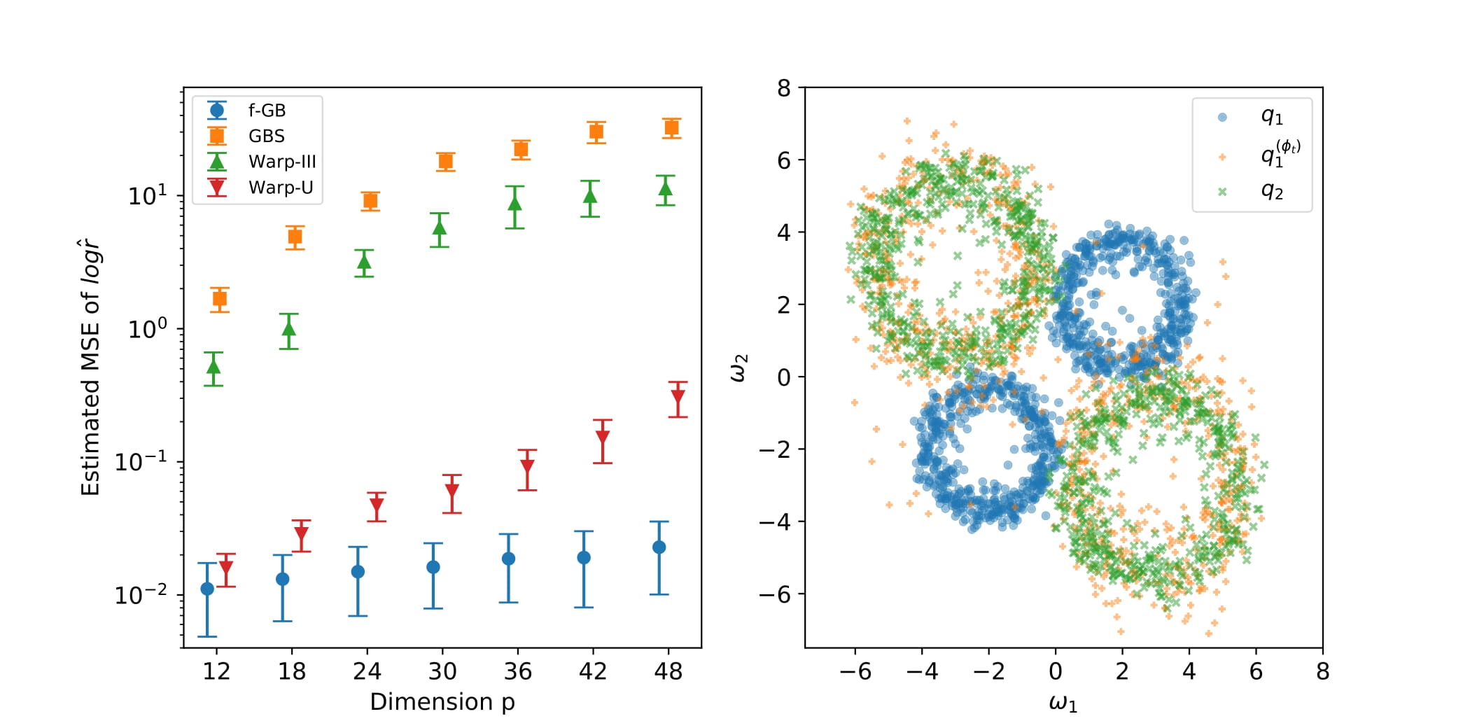
Figure 1: Left: MC estimates of MSE of $\log\hat{r}$ for each methods. Vertical segments are $2\sigma$ error bars. Note that the y-axis is on log scale. Right: Scatter plot of the first two dimensions of samples from $q_{1},q_{2}$ and $q_{1}^{(\phi_{t})}$ when $p=48$. $q_{1}^{(\phi_{t})}$ is obtained from Algorithm 2 with $n_{i}=n^{\prime}_{i}=1000$ for $i=1,2$.

We now compare the computational cost of these methods. Recall that our Algorithm 2 utilizes GPU acceleration. Because of the difference in GPU and CPU computing, it is not straightforward to compare the computational cost of Algorithm 2 with GBS, Warp-III and Warp-U, which are CPU based, using benchmarks such as CPU seconds or number of function calls. We simply report the averaged running time for each method on our machine in Figure 2. Similar to Wang et al., (2020), we will also report the average “precision per second”, which is the reciprocal of the product of the running time and the estimated MSE of $\log\hat{r}$, for each method (higher precision per second means better efficiency). We see that for all methods, the computation time is approximately a linear function of the dimension $p$. Even though $f$-GB takes roughly twice longer to run compared to GBS and $30\sim 40$ times longer compared to Warp-III, it achieves the highest precision per second for all dimension $p$ we consider. In addition, we also run further simulations with larger sample sizes. We find that when $p=48$, Warp-U needs around $N_{1}=N_{2}=7500$ samples to reach a similar level of precision as $f$-GB based on $N_{1}=N_{2}=2000$ samples. In this case, Warp-U takes around $3\sim 4$ times longer to run compared to $f$-GB. For Warp-III and GBS, we further increase the sample size to $N_{1}=N_{2}=5\times 10^{4}$, but find that their performance is still worse than $f$-GB and Warp-U, and both take more than three times longer to run. For Warp-III and Warp-U, it is not obvious how they would benefit from GPU computation. Although GBS may benefit from GPU acceleration in principle, it would require careful implementation and optimization. Therefore we compare our Algorithm 2 to these methods based on their publicly available implementations.

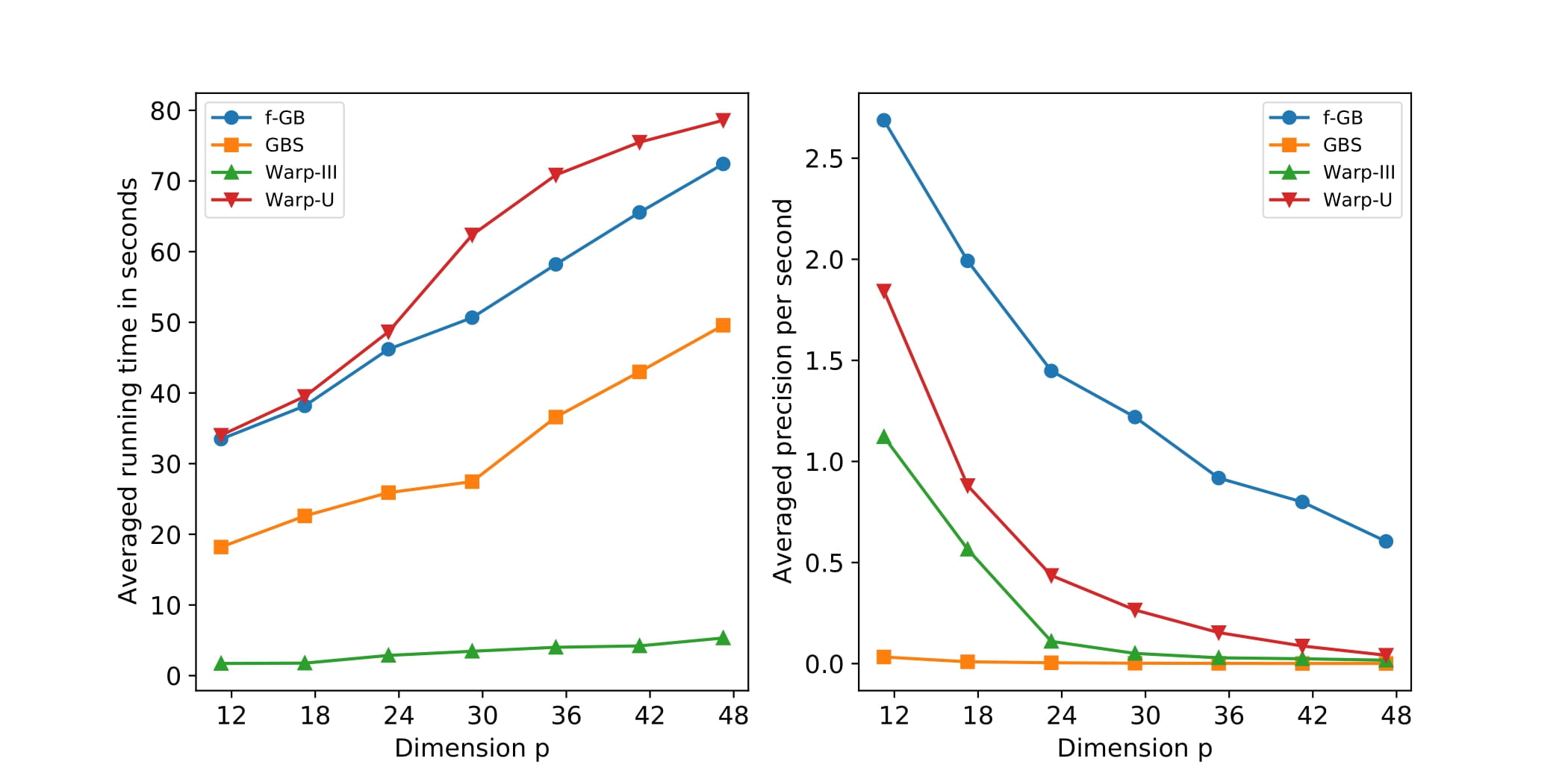
Figure 2: Left: Averaged running time for each method. Right: Averaged precision per second (i.e. reciprocal of the product of running time and the estimated MSE of $\log\hat{r}$) for each method.

Recall that $MSE(\log\hat{r}_{opt})$ is asymptotically equivalent to $RE^{2}(\hat{r}_{opt})$ (Meng and Wong,, 1996). Therefore $\widehat{RE}^{2}(\hat{r}^{\prime(\phi_{t})}_{opt})$ returned from Algorithm 2 can also be viewed as an estimate of $MSE(\log\hat{r}^{\prime(\phi_{t})}_{opt})$. In order to assess its accuracy, we compare it with both the error estimator given in Frühwirth-Schnatter, (2004) and a direct MC estimator of $MSE(\log\hat{r}^{\prime(\phi_{t})}_{opt})$: For each value of $p$, we first run Algorithm 2 with $N_{1}=N_{2}=2000$ samples as before (i.e. we set $n_{i}=n^{\prime}_{i}=1000$ for $i=1,2$). We then fix the transformed density $\tilde{q}^{(\phi_{t})}_{1}$ obtained from Algorithm 2, repeatedly draw $n^{\prime}_{1}=n^{\prime}_{2}=1000$ independent samples from $\tilde{q}^{(\phi_{t})}_{1},q_{2}$ and record $\hat{r}^{\prime(\phi_{t})}_{opt}$, $\widehat{RE}^{2}(\hat{r}^{\prime(\phi_{t})}_{opt})$ and the error estimate given in Frühwirth-Schnatter, (2004) (F-S) based on these new samples. We repeat this process 100 times, and report the box plots of $\widehat{RE}^{2}(\hat{r}^{\prime(\phi_{t})}_{opt})$ and the error estimates given in Frühwirth-Schnatter, (2004) (F-S) based on the repeated runs. We also compare the results with the direct MC estimate of $MSE(\log\hat{r}^{\prime(\phi_{t})}_{opt})$ based on the repeated estimates $\log\hat{r}^{\prime(\phi_{t})}_{opt}$ and the ground truth $\log r$. Note that here we fix the transformed $\tilde{q}^{(\phi_{t})}_{1}$ and only repeat the Bridge sampling step in Algorithm 2. We summarize the results in Figure 3. We see that $\widehat{RE}^{2}(\hat{r}^{\prime(\phi_{t})}_{opt})$ returned from Algorithm 2 agrees with the error estimator given in Frühwirth-Schnatter, (2004) (F-S), and provides a sensible estimate of $MSE(\log\hat{r}^{\prime(\phi_{t})}_{opt})$ for all choices of $p$.

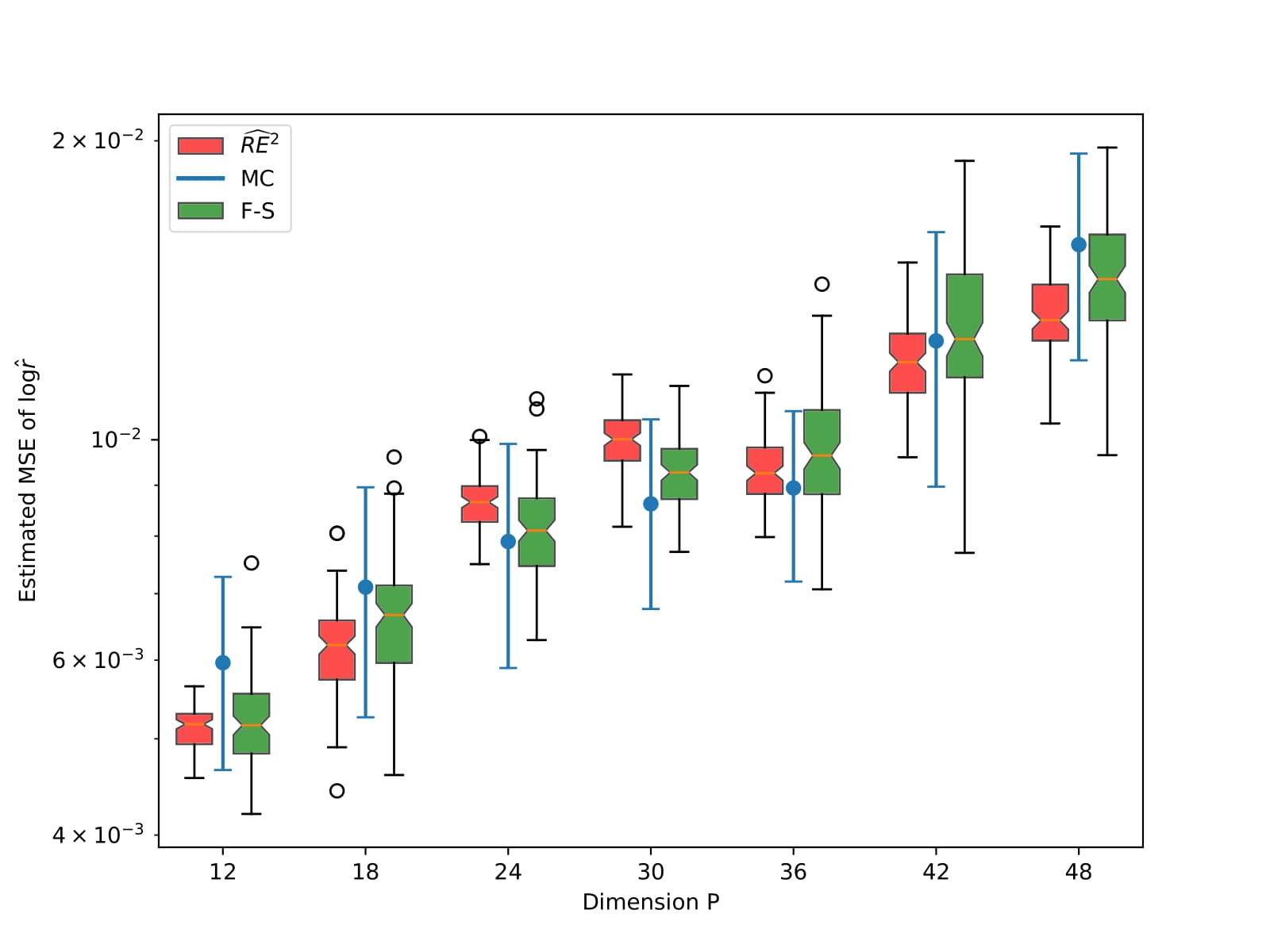
Figure 3: Box plots of 100 repetitions of $\widehat{RE}^{2}(\hat{r}^{\prime(\phi_{t})}_{opt})$ based on Algorithm 2 and the error estimator given in Frühwirth-Schnatter, (2004) (F-S) for each dimension $P$. Blue vertical segments are the $2\sigma$ error bars of the corresponding MC estimates of $MSE(\log\hat{r}^{\prime(\phi_{t})}_{opt})$ based on 100 repetitions.

6 Example 2: Comparing two Bayesian GLMMs

In this section we demonstrate the effectiveness of the $f$-GAN-Bridge estimator and Algorithm 2 by considering a Bayesian model comparison problem based on the six cities dataset (Fitzmaurice and Laird,, 1993), where $q_{1},q_{2}$ are the posterior densities of the parameters of two Bayesian GLMMs $M_{1},M_{2}$. This example is adapted from Overstall and Forster, (2010). We choose this example because it is based on real world dataset, and the posteriors $q_{1},q_{2}$ are relatively high dimensional and are defined on disjoint supports with different dimensions.

The six cities dataset consists of the wheezing status $y_{ij}$ (1 = wheezing, 0 otherwise) of child $i$ at time $j$ for $i=1,...,n$, $n=537$ and $j=1,...4$. It also includes $x_{ij}$, the smoking status (1 = smoke, 0 otherwise) of the $i$-th child’s mother at time-point $j$ as a covariate. We compare two mixed effects logistic regression models $M_{1},M_{2}$ with different linear predictors. Define

$$M1:\eta_{ij}^{(1)} =\beta_{0}+u_{i};\quad u_{i}\stackrel{{\scriptstyle i.i.d.}}{{\sim}}N(0,\sigma^{2})$$ (29)

$$M2:\eta_{ij}^{(2)} =\beta_{0}+\beta_{1}x_{ij}+u_{i};\quad u_{i}\stackrel{{\scriptstyle i.i.d.}}{{\sim}}N(0,\sigma^{2})$$ (30)

where $\beta_{0},\beta_{1}$ are regression parameters, $u_{i}$ is the random effect of the $i$-th child and $\sigma^{2}$ controls the variance of the random effects. We use the default prior given by Overstall and Forster, (2010) for both models, i.e. we take $\beta_{0}\sim N(0,4)$, $\sigma^{-2}\sim\Gamma(0.5,0.5)$ for $M_{1}$ and $(\beta_{0},\beta_{1})\sim N(0,4n(\boldsymbol{X}^{T}\boldsymbol{X})^{-1})$, $\sigma^{-2}\sim\Gamma(0.5,0.5)$ for $M_{2}$ where $\boldsymbol{X}=[\boldsymbol{1}_{4n}^{T},(\boldsymbol{x}_{1},...,\boldsymbol{x}_{n})^{T}]$, $\boldsymbol{x}_{i}=(x_{i1},...,x_{i4})$ for $i=1,...,n$.

Let $\boldsymbol{y}=(\boldsymbol{y}_{1},...\boldsymbol{y}_{n})$ with $\boldsymbol{y}_{i}=(y_{i1},...,y_{i4})$. Let $\boldsymbol{u}=(u_{1},...u_{n})$ be the vector of random effects. Let $q_{1}(\beta_{0},\boldsymbol{u})=p(\beta_{0},\boldsymbol{u}|\boldsymbol{X},\boldsymbol{y},M_{1})$ be the marginal posterior of $(\beta_{0},\boldsymbol{u})$ under $M_{1}$, and $\tilde{q}_{1}(\beta_{0},\boldsymbol{u})$ be the corresponding unnormalized density. Let $q_{2}(\beta_{0},\beta_{1},\boldsymbol{u})$, $\tilde{q}_{2}(\beta_{0},\beta_{1},\boldsymbol{u})$ be defined in a similar fashion under $M_{2}$. Samples of $q_{1},q_{2}$ are obtained using MCMC package R2WinBUGS (Sturtz et al.,, 2005; Lunn et al.,, 2000). For $k=1,2$, the normalizing constant $Z_{k}$ of $\tilde{q}_{k}$ is the marginal likelihood under $M_{k}$. We first generate $2\times 10^{5}$ MCMC samples from $q_{1},q_{2}$ and estimate $\log Z_{1},\log Z_{2}$ using the method described in Overstall and Forster, (2010). The estimated log marginal likelihoods of $M_{1},M_{2}$ based on $2\times 10^{5}$ MCMC samples are $-808.139$ and $-809.818$ respectively. The results are consistent with the estimated log marginal likelihoods reported in Overstall and Forster, (2010) based on $5\times 10^{4}$ MCMC samples. We take them as the baseline “true values” of $\log Z_{1}$ and $\log Z_{2}$. See Overstall and Forster, (2010) for R codes and technical details.

Similar to the previous example, we use $f$-GB to estimate the log Bayes factor $\log r=\log Z_{1}-\log Z_{2}$ between $M_{1},M_{2}$. Note that $q_{1},q_{2}$ are defined on disjoint support $\mathbb{R}^{n+1},\mathbb{R}^{n+2}$ respectively. In order to apply our Algorithm 2 to this problem, we first augment $q_{1}$ using a standard Normal to match up the difference in dimension between $q_{1}$ and $q_{2}$: Let $q_{1,aug}(\beta_{0},\gamma,\boldsymbol{u})=q_{1}(\beta_{0},\boldsymbol{u})N(\gamma;0,1)$ be the augmented density where $N(\cdot;0,1)$ is the standard Normal pdf. Let $\tilde{q}_{1,aug}$ be the corresponding unnormalized augmented density. Note that $\tilde{q}_{1,aug}$ and $\tilde{q}_{1}$ have the same normalizing constant $Z_{1}$. We can then apply Algorithm 2 to $q_{1,aug}$ and $q_{2}$ since $q_{1,aug}$ and $q_{2}$ are now defined on a common support $\mathbb{R}^{n+2}$. We can sample from $q_{1,aug}$ by simply concatenating a sample $(\beta_{0},\boldsymbol{u})\sim q_{1}$ and a sample $\gamma\sim N(0,1)$.

Let $N_{k}$ be the number of MCMC samples drawn from $q_{k}$ for $k=1,2$. In this example, we compare the performance of the $f$-GAN-Bridge estimator with the Warp-III Bridge estimator and the Warp-U Bridge estimator as we increase the number of MCMC samples $N_{1},N_{2}$. We consider sample size $N=\{1000,2000,3000,4000,5000\}$. This is a challenging task since the sample size $N$ is limited compared to the dimension of the problem (Recall that $q_{1},q_{2}$ are defined on $\mathbb{R}^{n+1},\mathbb{R}^{n+2}$ respectively with $n=537$). For each choice of $N$, we repeatedly draw $N_{1}=N_{2}=N$ MCMC samples from $q_{1},q_{2}$ respectively and estimate the MSE of $\log\hat{r}$ for each method in the same way as in the previous example. For our Algorithm 2, we augment $q_{1}$ as described above, set $\lambda_{1},\lambda_{2}=0.1$ and $q_{1,aug}^{(\phi)}$ to be a Real-NVP with 10 coupling layers. For the Warp-U and Warp-III Bridge estimator, we still use the recommended or default settings. We do not include GBS in this example since we find that for all values of $N$, it does not converge for most of the repetitions. From Figure 4 we see our Algorithm 2 outperforms the Warp-III and the Warp-U Bridge estimator for all sample size $N$. We also include a scatter plot of the first two dimensions of samples from $q_{1,aug},q_{2}$ and the transformed $q^{(\phi_{t})}_{1,aug}$, where $q^{(\phi_{t})}_{1,aug}$ is obtained from Algorithm 2 with $N=3000$. We see $q^{(\phi_{t})}_{1,aug}$ an $q_{2}$ share much greater overlap than the original $q_{1,aug},q_{2}$. From Figure 5 we see for the same sample size $N$, the running time of $f$-GB is $4\sim 6$ times as long as Warp-III, and roughly $30\%\sim 40\%$ shorter than Warp-U. On the other hand, $f$-GB achieves the highest precision per second for all sample size $N$ in this example. We further increase the sample size $N$, and find that Warp-U requires around $10^{4}$ MCMC samples to reach a similar level of precision achieved by $f$-GB with $N=5000$ samples, and takes around $2$ times longer to run. Similarly, Warp-III requires around $8\times 10^{4}$ samples to get a similar level of precision, and takes around three times longer to run.

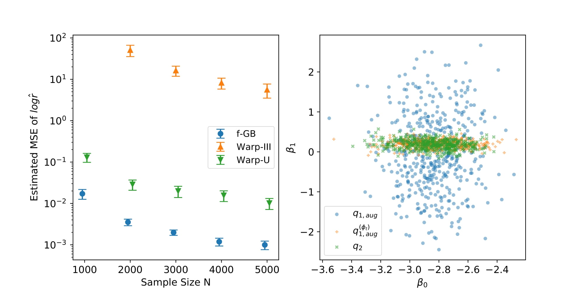
Figure 4: Left: MC estimates of MSE of $\log\hat{r}$ for each methods. Vertical segments are $2\sigma$ error bars. Note that the y-axis is on log scale. Warp-III does not converge for most of the repetitions when $N=1000$. Right: Scatter plot of the first two dimensions of samples from $q_{1,aug},q_{2}$ and $q_{1,aug}^{(\phi_{t})}$, where $q_{1,aug}^{(\phi_{t})}$ is obtained from Algorithm 2 with $n_{1}=n^{\prime}_{i}=1500$ for $i=1,2$. The first two dimensions of $q_{1,aug}$ and $q_{2}$ are $(\beta_{0},\gamma),(\beta_{0},\beta_{1})$ respectively.

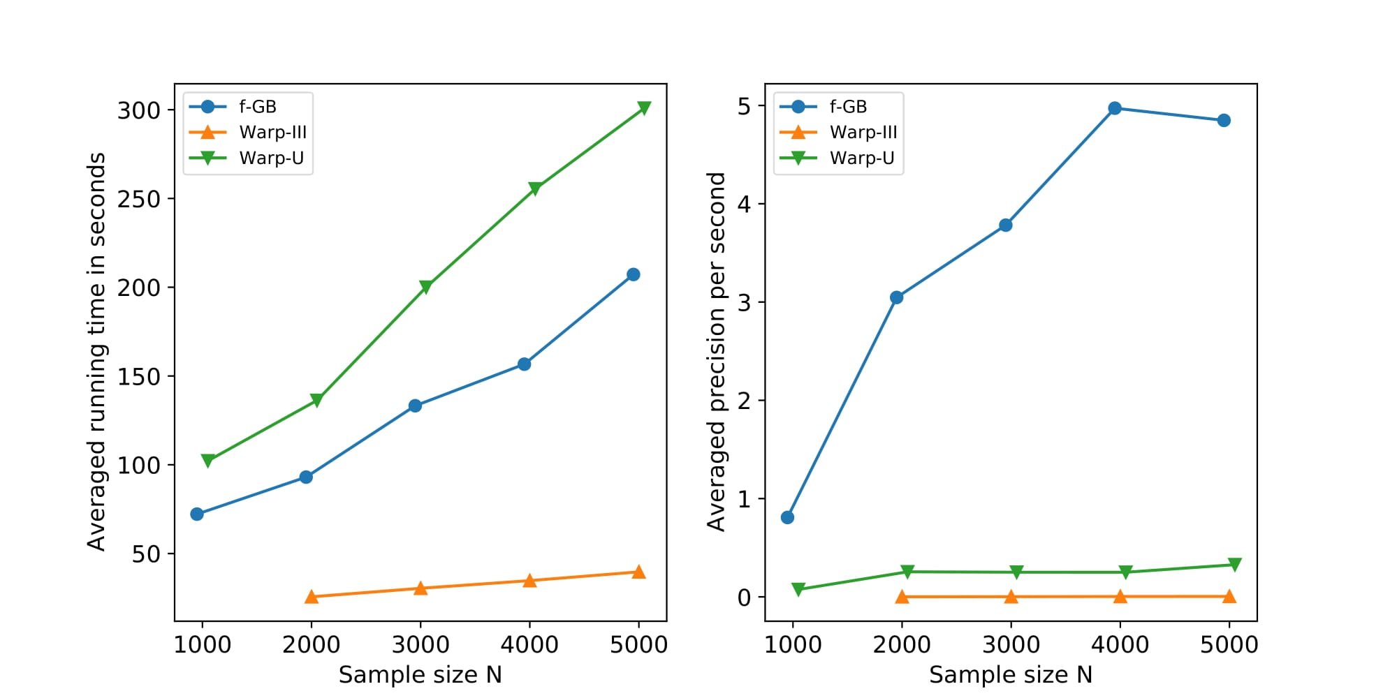
Figure 5: Left: Averaged running time for each method. Warp-III does not converge for most of the repetitions when $N=1000$. Right: Averaged precision per second (i.e. reciprocal of the product of running time and the estimated MSE of $\log\hat{r}$) for each method.

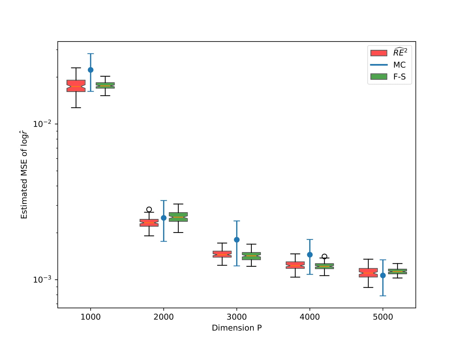
Figure 6: Box plots of 100 repetitions of $\widehat{RE}^{2}(\hat{r}^{\prime(\phi_{t})}_{opt})$ based on Algorithm 2 and the error estimator given in Frühwirth-Schnatter, (2004) (F-S) for each sample size $N$. Blue vertical segments are the $2\sigma$ error bars of the corresponding MC estimates of $MSE(\log\hat{r}^{\prime(\phi_{t})}_{opt})$ based on 100 repetitions.

For each choice of $N$, we also compare $\widehat{RE}^{2}(\hat{r}^{\prime(\phi_{t})}_{opt})$ returned from Algorithm 2 with the error estimator given in Frühwirth-Schnatter, (2004) (F-S) and a direct MC estimator of $MSE(\log\hat{r}^{\prime(\phi_{t})}_{opt})$ in the same way as in the last example. We summarize the results in Figure 6. In principle, it is not appropriate to use $\widehat{RE}^{2}(\hat{r}^{\prime(\phi_{t})}_{opt})$ as an estimate of $MSE(\log\hat{r}^{\prime(\phi_{t})}_{opt})$ in this example as the MCMC samples are correlated. However, from Figure 6 we see it agrees with the erorr estimator given in Frühwirth-Schnatter, (2004), which does take autocorrelation into account, and still provides sensible estimate of $MSE(\log\hat{r}^{\prime(\phi_{t})}_{opt})$ for all choices of $N$. This is likely due to the fact that the autocorrelation in our MCMC samples is weak, as we find that for all $N$, the effective sample sizes for all dimensions of the MCMC samples from $q_{1},q_{2}$ are greater than $0.8N$. When working with weakly correlated MCMC samples, we recommend users to compute both our $\widehat{RE}^{2}(\hat{r}^{\prime(\phi_{t})}_{opt})$ and the error estimator given in Frühwirth-Schnatter, (2004), which does take autocorrelation into account, and check if they agree with each other. When the MCMC samples are strongly correlated, we do not recommend using $\widehat{RE}^{2}(\hat{r}^{\prime(\phi_{t})}_{opt})$ as the error estimate of $\hat{r}^{\prime(\phi_{t})}_{opt}$.

7 Conclusion

In this paper, we give a new estimator of $RE^{2}(\hat{r}_{opt})$ based on the variational lower bound of $f$-divergence proposed by Nguyen et al., (2010), discuss the connection between Bridge estimators and the problem of $f$-divergence estimation, and give a computational framework to improve the optimal Bridge estimator using an $f$-GAN (Nowozin et al.,, 2016). We show that under the i.i.d. assumption, our $f$-GAN-Bridge estimator is optimal in the sense that it asymptotically minimizes the first order approximation of $RE^{2}(\hat{r}_{opt}^{(\phi)})$ with respect to the transformed density $q_{1}^{(\phi)}$. We see that in both simulated and real world examples, our $f$-GB estimator provides accurate estimate of $r$ and outperforms existing methods significantly. In addition, Algorithm 2 also provides accurate estimates of $RE^{2}(\hat{r}_{opt}^{(\phi)})$ and $MSE(\log\hat{r}_{opt}^{(\phi)})$. In our experience, Algorithm 2 ($f$-GB) is computationally more demanding than the existing methods. In the numerical examples, the running time of Algorithm 2 is roughly 1 to 3 times as long as the existing methods such as Warp-U and GBS when the sample size are the same. We have not attempted to formalize the difference in computational cost because of the very different nature of GPU and CPU computing. Although in our examples, it is possible for a competing method to match the performance of the $f$-GB estimator by increasing the number of samples drawn from $q_{1},q_{2}$, it takes longer to run, and can be inefficient or impractical when sampling from $q_{1},q_{2}$ is computationally expensive. This also means the $f$-GB estimator is especially appealing when we only have a limited amount of samples from $q_{1},q_{2}$. In summary, when $q_{1},q_{2}$ are relatively simple-structured and low dimensional, the extra computational cost required by $f$-GB may not be worthwhile. However, when $q_{1},q_{2}$ are high dimensional or have complicated multi-modal structure, we recommend the users to choose the more accurate $f$-GB estimator of $r$, given the key summary role it plays in many applications and publications.

7.1 Limitations and future works

One limitation of the $f$-GB estimator is the computational cost. In this paper we parameterize $q_{1}^{(\phi)}$ as a Normalizing flow. A possible direction of future work is to explore different choices of parameterizations of $q_{1}^{(\phi)}$. We expect that we can speed up our Algorithm 2 by replacing a Normalizing flow by simpler transformations such as Warp-I and Warp-II transformation (Meng and Schilling,, 2002) at the expense of flexibility. Another limitation is that Algorithm 1 is only optimal when samples from $q_{1},q_{2}$ are i.i.d. Recall that $RE^{2}(\hat{r}_{opt})$ in (13) is derived based on the i.i.d. assumption. Therefore if the samples from $q_{1},q_{2}$ are correlated, then Proposition 3 no longer holds, and minimizing $H_{s_{2}}(q_{1}^{(\phi)},q_{2})$ with respect to $q_{1}^{(\phi)}$ is no longer equivalent to minimizing the first order approximation of $RE^{2}(\hat{r}^{(\phi)}_{opt})$. Therefore it is of interest to see if it is possible to give an algorithm that minimizes the first order approximation of $RE^{2}(\hat{r}^{(\phi)}_{opt})$ when the samples are correlated. In addition, our approach only focuses on estimating the ratio of normalizing constants between two densities. When we have multiple unnormalized densities and would like to estimate the ratios between their normalizing constants, our approach needs to estimate these quantities separately in a pairwise fashion, which can be inefficient. Meng and Schilling, (1996) and (Geyer,, 1994) show that one can estimate multiple normalizing constants simultaneously up to a common multiplicative constant. We are also interested in extending our improvement strategy to this multiple densities setup.

SUPPLEMENTARY MATERIAL

8 Proofs

Here we give proof of Proposition 1, 2 and 3.

Proposition 1 (Estimating $H_{\pi}(q_{1},q_{2})$).

Let $q_{1},q_{2}$ be continuous densities with respect to a base measure $\mu$ on the common support $\Omega$. Let $\{\omega_{ij}\}_{j=1}^{n_{i}}$ be samples from $q_{i}$ for $i=1,2$. Let $\pi\in(0,1)$ be the weight parameter. Let $r$ be the true ratio of normalizing constants between $q_{1},q_{2}$, and $C_{2}>C_{1}>0$ be constants such that $r\in[C_{1},C_{2}]$. For $\tilde{r}\in[C_{1},C_{2}]$, define

$$G(\tilde{r};\pi)=1-\frac{1}{\pi}E_{q_{1}}\left(\frac{\pi\tilde{q}_{2}(\omega)\tilde{r}}{(1-\pi)\tilde{q}_{1}(\omega)+\pi\tilde{q}_{2}(\omega)\tilde{r}}\right)^{2}-\frac{1}{1-\pi}E_{q_{2}}\left(\frac{(1-\pi)\tilde{q}_{1}(\omega)}{(1-\pi)\tilde{q}_{1}(\omega)+\pi\tilde{q}_{2}(\omega)\tilde{r}}\right)^{2}.$$ (31)

Then $H_{\pi}(q_{1},q_{2})$ satisfies

$$H_{\pi}(q_{1},q_{2})\geq\sup_{\tilde{r}\in[C_{1},C_{2}]}G(\tilde{r};\pi),$$ (32)

and equality holds if and only if $\tilde{r}=r$. In addition, let $\hat{G}(\tilde{r};\pi,\{\omega_{ij}\}_{j=1}^{n_{i}})$ be an empirical estimate of $G(\tilde{r};\pi)$ based on $\{\omega_{ij}\}_{j=1}^{n_{i}}\sim q_{i}$ for $i=1,2$. If $\hat{r}_{\pi}=\operatorname*{arg\,max}_{\tilde{r}\in[C_{1},C_{2}]}\hat{G}(\tilde{r};\pi,\{\omega_{ij}\}_{j=1}^{n_{i}})$, then $\hat{r}_{\pi}$ is a consistent estimator of $r$, and $\hat{G}(\hat{r}_{\pi};\pi,\{\omega_{ij}\}_{j=1}^{n_{i}})$ is a consistent estimator of $H_{\pi}(q_{1},q_{2})$ as $n_{1},n_{2}\rightarrow\infty$.

Proof.

By definition, we know $0\leq H_{\pi}(q_{1},q_{2})\leq 1$. And by setting $D_{f}(q_{1},q_{2})=H_{\pi}(q_{1},q_{2})$, $f(u)=1-\frac{u}{\pi+(1-\pi)u}$ and variational function $V_{\tilde{r}}(\omega)=f^{\prime}\left(\frac{\tilde{q}_{1}(\omega)}{\tilde{q}_{2}(\omega)\tilde{r}}\right)$ with $\mathcal{V}=\{V_{\tilde{r}}(\omega)|\tilde{r}\in[C_{1},C_{2}]\}$, we see $G(\tilde{r};\pi)$ exists for all $\tilde{r}\in[C_{1},C_{2}]$ and is the variational lower bound of $H_{\pi}(q_{1},q_{2})$ in the form of (15). Then by Nguyen et al., (2010), equality holds if and only if $V_{\tilde{r}}(\omega)=f^{\prime}\left(\frac{\tilde{q}_{1}(\omega)}{\tilde{q}_{2}(\omega)r}\right)$. Since $f(u)$ is strictly convex, $f^{\prime}(u)$ is monotonically increasing. By assumption, we also know $q_{1}(\omega),q_{2}(\omega)>0$ for all $\omega\in\Omega$. Therefore by applying the inverse of $f^{\prime}$ to both side, we see $V_{\tilde{r}}(\omega)=f^{\prime}\left(\frac{\tilde{q}_{1}(\omega)}{\tilde{q}_{2}(\omega)r}\right)$ if and only if $\tilde{r}=r$. Therefore $G(r;\pi)=H_{\pi}(q_{1},q_{2})$, and $\tilde{r}=r$ is the unique maximizer of $G(\tilde{r};\pi)$.

Now we show the consistency of $\hat{r}_{\pi}$. It can be shown in a similar fashion to the proof of the consistency of an extremum estimator in e.g. Newey and McFadden, (1994) Theorem 2.1.

We first check $\hat{G}(\tilde{r};\pi,\{\omega_{ij}\}_{j=1}^{n_{i}})$ satisfies the uniform law of large number (ULLN). Let

$$g_{1}(\omega,\tilde{r})=\frac{1}{\pi}\left(\frac{\pi\tilde{q}_{2}(\omega)\tilde{r}}{(1-\pi)\tilde{q}_{1}(\omega)+\pi\tilde{q}_{2}(\omega)\tilde{r}}\right)^{2}$$

and

$$g_{2}(\omega,\tilde{r})=\frac{1}{1-\pi}\left(\frac{(1-\pi)\tilde{q}_{1}(\omega)}{(1-\pi)\tilde{q}_{1}(\omega)+\pi\tilde{q}_{2}(\omega)\tilde{r}}\right)^{2}.$$

Since $0<g_{1}(\omega,\tilde{r}),g_{2}(\omega,\tilde{r})<\max(\frac{1}{\pi},\frac{1}{1-\pi})$ for any $\omega\in\Omega$ and $\tilde{r}\in[C_{1},C_{2}]$, by Jennrich, (1969) Theorem 2, we have

$$\sup_{\tilde{r}\in[C_{1},C_{2}]}\left|\frac{1}{n_{1}}\sum_{j=1}^{n_{1}}g_{1}(\omega_{1j})-E_{q_{1}}g_{1}(\omega,\tilde{r})\right|\rightarrow_{p}0$$

and

$$\sup_{\tilde{r}\in[C_{1},C_{2}]}\left|\frac{1}{n_{2}}\sum_{j=1}^{n_{2}}g_{2}(\omega_{2j})-E_{q_{2}}g_{2}(\omega,\tilde{r})\right|\rightarrow_{p}0$$

as $n_{1},n_{2}\rightarrow\infty$. Since $G(\tilde{r};\pi)=1-E_{q_{1}}g_{1}(\omega,\tilde{r})-E_{q_{2}}g_{2}(\omega,\tilde{r})$, by triangle inequality, we have

$$\sup_{\tilde{r}\in[C_{1},C_{2}]}\left|\hat{G}(\tilde{r};\pi,\{\omega_{ij}\}_{j=1}^{n_{i}})-G(\tilde{r};\pi)\right|\rightarrow_{p}0$$

as $n_{1},n_{2}\rightarrow\infty$. Hence $\hat{G}(\tilde{r};\pi,\{\omega_{ij}\}_{j=1}^{n_{i}})$ satisfies the uniform law of large number (ULLN).

We also need to check $G(\hat{r}_{\pi};\pi)\rightarrow_{p}G(r;\pi)$:

$$G(r;\pi) \geq G(\hat{r}_{\pi};\pi)\quad\mbox{since $r$ is the unique maximizer of $G(\tilde{r};\pi)$}$$ (33)

$$=\hat{G}(\hat{r}_{\pi};\pi,\{\omega_{ij}\}_{j=1}^{n_{i}})+(G(\hat{r}_{\pi};\pi)-\hat{G}(\hat{r}_{\pi};\pi,\{\omega_{ij}\}_{j=1}^{n_{i}}))$$ (34)

$$\geq\hat{G}(r;\pi,\{\omega_{ij}\}_{j=1}^{n_{i}})+(G(\hat{r}_{\pi};\pi)-\hat{G}(\hat{r}_{\pi};\pi,\{\omega_{ij}\}_{j=1}^{n_{i}}))$$ (35)

$$=G(r;\pi)+(\hat{G}(r;\pi,\{\omega_{ij}\}_{j=1}^{n_{i}})-G(r;\pi))+(G(\hat{r}_{\pi};\pi)-\hat{G}(\hat{r}_{\pi};\pi,\{\omega_{ij}\}_{j=1}^{n_{i}}))$$ (36)

Since the last two terms converge in probability to 0 by ULLN, we have $G(r;\pi)\geq G(\hat{r}_{\pi};\pi)\geq G(r;\pi)+o_{p}(1)$. This implies $G(\hat{r}_{\pi};\pi)\rightarrow_{p}G(r;\pi)$.

Since $[C_{1},C_{2}]$ is compact and $G(\tilde{r};\pi)$ is continuous, for every open interval $A\subset[C_{1},C_{2}]$ containing $r$, we have $\sup_{\tilde{r}\not\in A}G(\tilde{r};\pi)<G(r;\pi)$. On the other hand, $G(\hat{r}_{\pi};\pi)\rightarrow_{p}G(r;\pi)$ implies that $Pr(G(\hat{r}_{\pi};\pi)>\sup_{\tilde{r}\not\in A}G(\tilde{r};\pi))$ converges to 1. Therefore $Pr(\hat{r}_{\pi}\in A)$ also converges to 1, i.e. $\hat{r}_{\pi}$ is a consistent estimator of $r$.

Finally we show $\hat{G}(\hat{r}_{\pi};\pi,\{\omega_{ij}\}_{j=1}^{n_{i}})$ is a consistent estimator of $H_{\pi}(q_{1},q_{2})$. Recall that $G(r;\pi)=H_{\pi}(q_{1},q_{2})$. By triangle inequality,

$$\left|\hat{G}(\hat{r}_{\pi};\pi,\{\omega_{ij}\}_{j=1}^{n_{i}})-H_{\pi}(q_{1},q_{2})\right| \leq\left|\hat{G}(\hat{r}_{\pi};\pi,\{\omega_{ij}\}_{j=1}^{n_{i}})-G(\hat{r}_{\pi};\pi)\right|+\left|G(\hat{r}_{\pi};\pi)-G(r;\pi)\right|$$ (37)

The first term on the RHS converges to 0 in probability by ULLN. The second term on the RHS converges to 0 in probability by continuous mapping theorem and the fact that $\hat{r}_{\pi}$ is a consistent estimator of $r$. Hence $\hat{G}(\hat{r}_{\pi};\pi,\{\omega_{ij}\}_{j=1}^{n_{i}})$ is a consistent estimator of $H_{\pi}(q_{1},q_{2})$. ∎

Proposition 2 (Connection between $\hat{r}^{(f)}$ and Bridge sampling).

Suppose $f(u):\mathbb{R}^{+}\to\mathbb{R}$ is strictly convex, twice differentiable and satisfies $f(1)=0$. Let $\{\omega_{ij}\}_{j=1}^{n_{i}}$ be samples from $q_{i}$ for $i=1,2$. If $\hat{r}^{(f)}=\operatorname*{arg\,max}_{\tilde{r}\in\mathbb{R}^{+}}\hat{G}_{f}(\tilde{r};\{\omega_{ij}\}_{j=1}^{n_{i}})$ is a stationary point of $\hat{G}_{f}(\tilde{r};\{\omega_{ij}\}_{j=1}^{n_{i}})$ in (21), then $\hat{r}^{(f)}$ satisfies the following equation

$$\hat{r}^{(f)}=\frac{\frac{1}{n_{2}}\sum_{j=1}^{n_{2}}f^{\prime\prime}\left(\frac{\tilde{q}_{1}(\omega_{2j})}{\tilde{q}_{2}(\omega_{2j})\hat{r}^{(f)}}\right)\frac{\tilde{q}_{1}(\omega_{2j})}{\tilde{q}_{2}(\omega_{2j})^{2}}\tilde{q}_{1}(\omega_{2j})}{\frac{1}{n_{1}}\sum_{j=1}^{n_{1}}f^{\prime\prime}\left(\frac{\tilde{q}_{1}(\omega_{1j})}{\tilde{q}_{2}(\omega_{1j})\hat{r}^{(f)}}\right)\frac{\tilde{q}_{1}(\omega_{1j})}{\tilde{q}_{2}(\omega_{1j})^{2}}\tilde{q}_{2}(\omega_{1j})}.$$ (38)

where $f^{\prime\prime}$ is the second order derivative of $f$.

Proof.

Note that the objective function can be written as

$$\hat{G}_{f}(\tilde{r};\{\omega_{ij}\}_{j=1}^{n_{i}}) =\frac{1}{n_{1}}\sum_{j=1}^{n_{1}}f^{\prime}\left(\frac{\tilde{q}_{1}(\omega_{1j})}{\tilde{q}_{2}(\omega_{1j})\tilde{r}}\right)-\frac{1}{n_{2}}\sum_{j=1}^{n_{2}}f^{*}\circ f^{\prime}\left(\frac{\tilde{q}_{1}(\omega_{2j})}{\tilde{q}_{2}(\omega_{2j})\tilde{r}}\right)$$ (39)

$$=\frac{1}{n_{1}}\sum_{j=1}^{n_{1}}f^{\prime}\left(\frac{\tilde{q}_{1}(\omega_{1j})}{\tilde{q}_{2}(\omega_{1j})\tilde{r}}\right)-\frac{1}{n_{2}}\sum_{j=1}^{n_{2}}\frac{\tilde{q}_{1}(\omega_{2j})}{\tilde{q}_{2}(\omega_{2j})\tilde{r}}f^{\prime}\left(\frac{\tilde{q}_{1}(\omega_{2j})}{\tilde{q}_{2}(\omega_{2j})\tilde{r}}\right)-f\left(\frac{\tilde{q}_{1}(\omega_{2j})}{\tilde{q}_{2}(\omega_{2j})\tilde{r}}\right)$$ (40)

using the equation $f^{*}\circ f^{\prime}(u)=uf^{\prime}(u)-f(u)$ (Uehara et al.,, 2016). Let $S(\tilde{r};\{\omega_{ij}\}_{j=1}^{n_{i}})=\frac{d}{d\tilde{r}}\hat{G}_{f}(\tilde{r};\{\omega_{ij}\}_{j=1}^{n_{i}})$. If $\hat{r}^{(f)}$ is the stationary point, then it satisfies the “score” equation

$$0 =S(\hat{r}^{(f)};\{\omega_{ij}\}_{j=1}^{n_{i}})$$ (41)

$$=-\frac{1}{n_{1}}\sum_{j=1}^{n_{1}}f^{\prime\prime}\left(\frac{\tilde{q}_{1}(\omega_{1j})}{\tilde{q}_{2}(\omega_{1j})\hat{r}^{(f)}}\right)\frac{\tilde{q}_{1}(\omega_{1j})}{\tilde{q}_{2}(\omega_{1j})(\hat{r}^{(f)})^{2}}+\frac{1}{n_{2}}\sum_{j=1}^{n_{2}}f^{\prime\prime}\left(\frac{\tilde{q}_{1}(\omega_{2j})}{\tilde{q}_{2}(\omega_{2j})\hat{r}^{(f)}}\right)\frac{\tilde{q}_{1}(\omega_{2j})^{2}}{\tilde{q}_{2}(\omega_{2j})^{2}(\hat{r}^{(f)})^{3}}$$ (42)

The above equation can be rearranged as

$$\hat{r}^{(f)}=\frac{\frac{1}{n_{2}}\sum_{j=1}^{n_{2}}f^{\prime\prime}\left(\frac{\tilde{q}_{1}(\omega_{2j})}{\tilde{q}_{2}(\omega_{2j})\hat{r}^{(f)}}\right)\frac{\tilde{q}_{1}(\omega_{2j})}{\tilde{q}_{2}(\omega_{2j})^{2}}\tilde{q}_{1}(\omega_{2j})}{\frac{1}{n_{1}}\sum_{j=1}^{n_{1}}f^{\prime\prime}\left(\frac{\tilde{q}_{1}(\omega_{1j})}{\tilde{q}_{2}(\omega_{1j})\hat{r}^{(f)}}\right)\frac{\tilde{q}_{1}(\omega_{1j})}{\tilde{q}_{2}(\omega_{1j})^{2}}\tilde{q}_{2}(\omega_{1j})}$$ (43)

∎

Proposition 3 (Minimizing $RE^{2}(\hat{r}^{(\phi)}_{opt})$ using Algorithm 1).

If $(\phi^{*},\tilde{r}^{*})$ is the solution of $\min_{\phi\in\mathbb{R}^{l}}\max_{\tilde{r}\in\mathbb{R}^{+}}G(\phi,\tilde{r};s_{2})$ defined in Algorithm 1, then $G(\phi,\tilde{r}^{*};s_{2})=H_{s_{2}}(q_{1}^{(\phi)},q_{2})$ for all $\phi\in\mathbb{R}^{l}$, $T_{\phi^{*}}$ minimizes $H_{s_{2}}(q_{1}^{(\phi)},q_{2})$ with respect to $T_{\phi}\in\mathcal{T}$. If the samples $\{\omega_{ij}\}_{j=1}^{n_{i}}\overset{i.i.d.}{\sim}q_{i}$ for $i=1,2$, then $T_{\phi^{*}}$ also minimizes $RE^{2}(\hat{r}^{(\phi)}_{opt})$ with respect to $T_{\phi}\in\mathcal{T}$ up to the first order.

Proof.

For every $\phi\in\mathbb{R}^{l}$, $G(\phi,\tilde{r};s_{2})$ is the variational lower bound of $H_{s_{2}}(q_{1}^{(\phi)},q_{2})$ in the form of (15). By Proposition 1, we know $G(\phi,\tilde{r};s_{2})$ is uniquely maximized at $\tilde{r}=r$ w.r.t $\tilde{r}>0$, and $G(\phi,r;s_{2})=H_{s_{2}}(q_{1}^{(\phi)},q_{2})$. Since $(\phi^{*},\tilde{r}^{*})$ is the solution of $\min_{\phi\in\mathbb{R}^{l}}\max_{\tilde{r}\in\mathbb{R}^{+}}G(\phi,\tilde{r};s_{2})$, it is straightforward to verify that $\tilde{r}^{*}=r$, and $H_{s_{2}}(q_{1}^{(\phi^{*})},q_{2})=G(\phi^{*},\tilde{r}^{*};s_{2})\leq G(\phi,\tilde{r}^{*};s_{2})$ for any $\phi\in\mathbb{R}^{l}$. Hence $T_{\phi^{*}}$ minimizes $H_{s_{2}}(q_{1}^{(\phi)},q_{2})$ with respect to $T_{\phi}\in\mathcal{T}$.

Since the leading term of $RE^{2}(\hat{r}^{(\phi)}_{opt})$ in (13) is a monotonically increasing function of $H_{s_{2}}(q_{1}^{(\phi)},q_{2})$, $T_{\phi^{*}}$ minimizes $H_{s_{2}}(q_{1}^{(\phi)},q_{2})$ w.r.t. $T_{\phi}\in\mathcal{T}$ implies $T_{\phi^{*}}$ minimizes the leading term of $RE^{2}(\hat{r}^{(\phi)}_{opt})$ w.r.t. $T_{\phi}\in\mathcal{T}$ under the assumption that samples $\{\omega_{ij}\}_{j=1}^{n_{i}}\sim q_{i}$ are i.i.d. for $i=1,2$. ∎

9 Dimension matching

The standard Bridge estimator (1) can not be applied directly when $\Omega_{1}$,$\Omega_{2}$ have different dimensions. This is a common and important case. For example, if we would like to compare two models $M_{1},M_{2}$ by estimating the Bayes factor between them, the standard Bridge estimator (1) is not directly applicable when $M_{1},M_{2}$ are controlled by parameters that live in different dimensions.

Assume $\Omega_{1}=\mathbb{R}^{d_{1}}$, $\Omega_{2}=\mathbb{R}^{d_{2}}$ and $d_{1}<d_{2}$. Discrete cases work similarly. Chen and Shao, (1997) resolve the problem of unequal dimensions by first augmenting the lower dimensional density $q_{1}(\omega_{1})$ by some completely known, normalized density $p(\theta|\omega_{1})$ where $\theta\in\mathbb{R}^{d_{2}-d_{1}}$. This ensures the augmented density

$$q_{1}^{*}(\omega_{1},\theta) =\tilde{q}_{1}^{*}(\omega_{1},\theta)/Z_{1}$$ (44)

$$=\tilde{q}_{1}(\omega_{1})p(\theta|\omega_{1})/Z_{1}$$ (45)

matches the dimension of the $q_{2}$, where $\tilde{q}_{1}^{*}(\omega_{1},\theta)$ is the unnormalized augmented density. Let $\Omega_{1}^{*}$ be the augmented support of $q_{1}^{*}$. Since the augmented density $q_{1}^{*}(\omega_{1},\theta)$ and the original $q_{1}(\omega_{1})$ have the same normalizing constant, we can then treat $r=Z_{1}/Z_{2}$ as the ratio between the normalizing constants of $q_{1}^{*}(\omega_{1},\theta)$ and $q_{2}(\omega_{2})$, and form an “augmented” Bridge estimator $\hat{r}^{*}_{\alpha}$ based on the augmented densities. Chen and Shao, (1997) also show that when the free function $\alpha(\omega)=\alpha_{opt}(\omega)$, the optimal augmenting density $p_{opt}(\theta|\omega_{1})$ which attains the minimal $RE^{2}(\hat{r}^{*}_{\alpha_{opt}})$ is

$$p_{opt}(\theta|\omega_{1})=q_{2}(\theta|\omega_{1})$$ (46)

i.e. $p_{opt}(\theta|\omega_{1})$ is the conditional distribution of the remaining $d_{2}-d_{1}$ entries of $\omega_{2}\sim q_{2}$ given that the first $d_{1}$ entries are $\omega_{1}$. However, $q_{2}(\theta|\omega_{1})$ is difficult to evaluate or sample from in general. One way to approximate the optimal augmenting distribution $q_{2}(\theta|\omega_{1})$ is to incorporate the augmented density $q_{1}^{*}(\omega_{1},\theta)$ with a Normalizing flow (see Sec 2.1). Assume we start with an arbitrary augmenting density $p(\theta|\omega_{1})$, e.g. standard Normal $N(0,I_{d_{2}-d_{1}})$. Consider a Normalizing flow with base density $q_{1}^{*}$ and a smooth and invertible transformation $T^{*}_{1}:\Omega_{1}^{*}\to\Omega_{2}$ that aims to map the augmented $q_{1}^{*}$ to the target $q_{2}$. Let $(\omega_{1}^{(T)},\theta^{(T)})=T^{*}_{1}(\omega_{1},\theta)$. If $q_{1}^{*(T)}(\omega_{1}^{(T)},\theta^{(T)})\approx q_{2}(\omega_{1}^{(T)},\theta^{(T)})$ for all $(\omega_{1}^{(T)},\theta^{(T)})\in\Omega_{2}$, i.e. $q_{1}^{*(T)}$ is a good approximation to $q_{2}$, then for the transformed augmenting density, we expect $q_{1}^{*(T)}(\theta^{(T)}|\omega_{1}^{(T)})\approx q_{2}(\theta^{(T)}|\omega_{1}^{(T)})$ as well. This means the transformed $q_{1}^{*(T)}$ automatically learns the optimal augmenting density.

10 Bias in the estimator of $H_{\pi}(q_{1},q_{2})$ given in Proposition 1

In Proposition 1, the estimator of $H_{\pi}(q_{1},q_{2})$ is given in the form of the maximum of the function $\hat{G}(\tilde{r};\pi,\{\omega_{ij}\}_{j=1}^{n_{i}})$ w.r.t. $\tilde{r}$. Let $r=Z_{1}/Z_{2}$ be the true ratio of normalizing constants. Even though $\hat{G}(r;\pi,\{\omega_{ij}\}_{j=1}^{n_{i}})$ is an unbiased estimator of $H_{\pi}(q_{1},q_{2})$, our proposed estimator $\hat{G}(\hat{r}_{\pi};\pi,\{\omega_{ij}\}_{j=1}^{n_{i}})$ sufferes from a positive bias. Intuitively speaking, this bias is analogous to the fact that the training error of a model is an underestimate of the true error. We use a toy example to illustrate this bias. Let $x\in\mathbb{R}^{3}$, $\sigma_{1}=1$ and $\sigma_{2}=3$. Let

$$\tilde{q}_{1}=\exp\left(-\frac{\left\lVert x\right\rVert^{2}_{2}}{2\sigma_{1}^{2}}\right)$$ (47)

$$\tilde{q}_{2}=\exp\left(-\frac{\left\lVert x\right\rVert^{2}_{2}}{2\sigma_{2}^{2}}\right).$$ (48)

In other words, $\tilde{q}_{1},\tilde{q}_{2}$ are the unnormalized pdf of two Gaussian distributions with zero mean and covaraince $\sigma_{1}I_{3},\sigma_{2}I_{3}$ respectively, where $I_{p}$ is the $p\times p$ identity matrix. Let $q_{1},q_{2}$ be the corresponding normalized densities. Let $\pi=0.5$. It is straightforward to form an unbiased MC estimate of $H_{\pi}(q_{1},q_{2})$ using (12). Let $N=\{10,20,30,...,1000\}$. For each value of $N$, we repeatedly compute the proposed estimator $\hat{G}(\hat{r}_{\pi};\pi,\{\omega_{ij}\}_{j=1}^{n_{i}})$ 1000 times based on $n_{1}=n_{2}=N$ i.i.d. samples from $q_{1},q_{2}$ respectively. We then report the sample mean of the repeated estimates for each $N$, and compare it with a high precision unbiased MC estimator of $H_{\pi}(q_{1},q_{2})$. From Figure 7 we see $\hat{G}(\hat{r}_{\pi};\pi,\{\omega_{ij}\}_{j=1}^{n_{i}})$ does exhibit a positive bias when $N<500$, and this bias gradually vanishes as sample size increases.

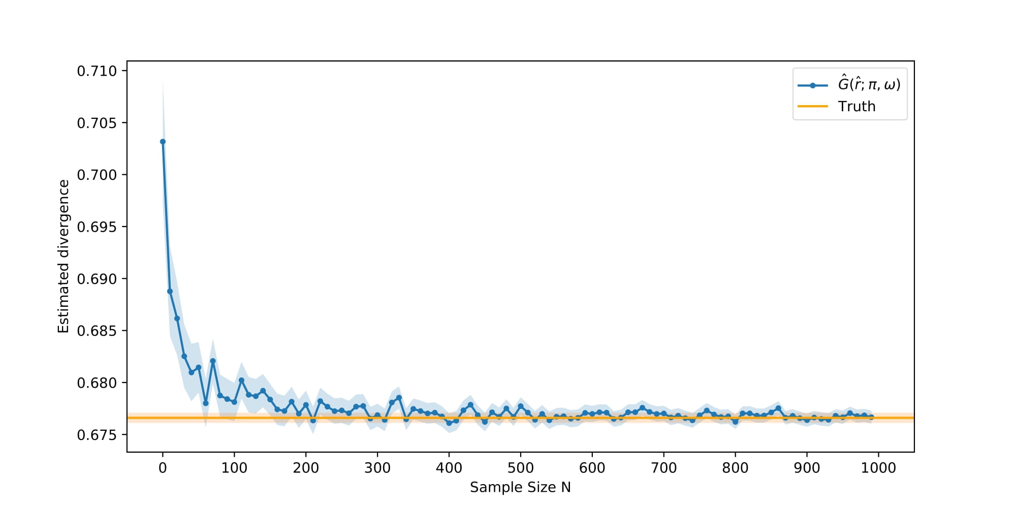
Figure 7: Sample mean of the estimated $H_{\pi}(q_{1},q_{2})$ for each sample size $N$. The blue band represents the $2\sigma$ error bars of the sample means. Orange line represents a high precision unbiased MC estimator of $H_{\pi}(q_{1},q_{2})$. Orange band represents the $2\sigma$ error bar of the MC estimate.

Even though we have not found a practical strategy to correct this bias, we believe this bias does not prevent our proposed estimator from being useful in practice. Since our estimator of $RE^{2}(\hat{r}_{opt})$ in (19) is a monotonically increasing function of $\hat{G}(\hat{r}_{\pi};\pi,\{\omega_{ij}\}_{j=1}^{n_{i}})$, the positive bias in $\hat{G}(\hat{r}_{\pi};\pi,\{\omega_{ij}\}_{j=1}^{n_{i}})$ leads to a positive bias in $\widehat{RE}^{2}(\hat{r}_{opt})$. Therefore $\widehat{RE}^{2}(\hat{r}_{opt})$ will systemically overestimate the true error $RE^{2}(\hat{r}_{opt})$, which will lead to more conservative conclusions (e.g. wider error bars). This is certainly not ideal, but we believe in practice, it is less harmful than underestimating the variability in $\hat{r}_{opt}$. In addition, we see that our proposed error estimator provides accurate estimates of the MSE of $\log\hat{r}^{\prime(\phi^{t})}_{opt}$ in both examples in Sec 5 and 6, indicating the effectiveness of it.

11 $f$-divergence and Bridge estimators

Here we give some examples of Proposition 2. We demonstrate how the Bridge estimators with different choices of free function $\alpha(\omega)$ arise from estimating different $f$-divergences.

Example 1 (KL divergence and the Importance sampling estimator)

KL divergence

$$KL(q_{1},q_{2})=\int_{\Omega}\log\left(\frac{q_{1}(\omega)}{q_{2}(\omega)}\right)q_{1}(\omega)d\mu(\omega)$$ (49)

is an $f$-divergence with $f(u)=u\log u$, $f^{\prime}(u)=1+\log u$ and $f^{*}(t)=\exp(t-1)$. This specification corresponds to $V_{\tilde{r}}(\omega)=1+\log\frac{\tilde{q}_{1}(x)}{\tilde{q}_{2}(x)\tilde{r}}$. Suppose we have $\{\omega_{1j}\}_{j=1}^{n_{1}}\sim q_{1}$ and $\{\omega_{2j}\}_{j=1}^{n_{2}}\sim q_{2}$. The maximizer $\hat{r}_{KL}$ of equation (20) under this specification is

$$\hat{r}_{KL} =\operatorname*{arg\,max}_{\tilde{r}\in\mathbb{R}^{+}}\frac{1}{n_{1}}\sum_{j=1}^{n_{1}}\left(1+\log\frac{\tilde{q}_{1}(\omega_{1j})}{\tilde{q}_{2}(\omega_{1j})\tilde{r}}\right)-\frac{1}{n_{2}}\sum_{j=1}^{n_{2}}\frac{\tilde{q}_{1}(\omega_{2j})}{\tilde{q}_{2}(\omega_{2j})\tilde{r}}$$ (50)

$$=\frac{1}{n_{2}}\sum_{j=1}^{n_{2}}\frac{\tilde{q}_{1}(\omega_{2j})}{\tilde{q}_{2}(\omega_{2j})}$$ (51)

Note that this is the Importance sampling estimator of $r$ using $q_{2}$ as the proposal, which is a special case of a Bridge estimator with free function $\alpha(\omega)=\tilde{q}_{2}(\omega)^{-1}$. Therefore we recover the Importance sampling estimator from the problem of estimating $KL(q_{1},q_{2})$. It is also straightforward to verify that estimating $KL(q_{2},q_{1})$ leads to $\hat{r}_{KL}=\left(\frac{1}{n_{1}}\sum_{j=1}^{n_{1}}\frac{\tilde{q}_{2}(\omega_{1j})}{\tilde{q}_{1}(\omega_{1j})}\right)^{-1}$, the Reciprocal Importance sampling estimator of $r$ based on a similar argument.

Example 2 (Weighted Jensen-Shannon divergence and the optimal Bridge estimator)

Weighted Jensen-Shannon divergence is defined as

$$JS_{\pi}(q_{1},q_{2})=\pi KL(q_{1},q_{\pi})+(1-\pi)KL(q_{2},q_{\pi})$$ (52)

where $\pi\in(0,1)$ is the weight parameter and $q_{\pi}=\pi q_{1}+(1-\pi)q_{2}$ is a mixture of $q_{1}$ and $q_{2}$. Weighted Jensen-Shannon divergence is an $f$-divergence with $f(u)=\pi u\log u-(1-\pi+\pi u)\log(1-\pi+\pi u)$, $f^{\prime}(u)=\pi\log\frac{u}{1-\pi+\pi u}$ and $f^{*}(t)=(1-\pi)\log\frac{1-\pi}{1-\pi\exp(t/\pi)}$. This corresponds to $V_{\tilde{r}}(\omega)=\pi\log\frac{\tilde{q}_{1}(\omega)}{\pi\tilde{q}_{1}(\omega)+(1-\pi)\tilde{q}_{2}(\omega)\tilde{r}}$. Suppose we have $\{\omega_{1j}\}_{j=1}^{n_{1}}\sim q_{1}$ and $\{\omega_{2j}\}_{j=1}^{n_{2}}\sim q_{2}$. Let the weight $\pi=\frac{n_{1}}{n_{1}+n_{2}}=s_{1}$, then under this specification, the maximizer $\hat{r}_{JS}$ of Equation (20) is defined as

$$\hat{r}_{JS}=\operatorname*{arg\,max}_{\tilde{r}\in\mathbb{R}^{+}}\frac{\pi}{n_{1}}\sum_{j=1}^{n_{1}}\log\frac{\tilde{q}_{1}(\omega_{1j})}{\pi\tilde{q}_{1}(\omega_{1j})+(1-\pi)\tilde{q}_{2}(\omega_{1j})\tilde{r}}\\ +\frac{1-\pi}{n_{2}}\sum_{j=1}^{n_{2}}\log\frac{\tilde{q}_{2}(\omega_{2j})\tilde{r}}{\pi\tilde{q}_{1}(\omega_{2j})+(1-\pi)\tilde{q}_{2}(\omega_{2j})\tilde{r}}$$ (53)

It is straightforward to verify that $\hat{r}_{JS}$ satisfies

$$\hat{r}_{JS}=\frac{\frac{1}{n_{2}}\sum_{j=1}^{n_{2}}\frac{\pi\tilde{q}_{1}(\omega_{2j})}{\pi\tilde{q}_{1}(\omega_{2j})+(1-\pi)\tilde{q}_{2}(\omega_{2j})\hat{r}_{JS}}}{\frac{1}{n_{1}}\sum_{j=1}^{n_{1}}\frac{(1-\pi)\tilde{q}_{2}(\omega_{1j})}{\pi\tilde{q}_{1}(\omega_{1j})+(1-\pi)\tilde{q}_{2}(\omega_{1j})\hat{r}_{JS}}}$$ (54)

On the other hand, recall that the asymptotically optimal Bridge estimator $\hat{r}_{opt}$ must be a fixed point of the iterative procedure (4). Therefore $\hat{r}_{opt}$ satisfies the following “score equation” (Meng and Wong,, 1996)

$$S(\hat{r}_{opt}) =-\sum_{j=1}^{n_{1}}\frac{s_{2}\tilde{q}_{2}(\omega_{1j})\hat{r}_{opt}}{s_{1}\tilde{q}_{1}(\omega_{1j})+s_{2}\tilde{q}_{2}(\omega_{1j})\hat{r}_{opt}}+\sum_{j=1}^{n_{2}}\frac{s_{1}\tilde{q}_{1}(\omega_{2j})}{s_{1}\tilde{q}_{1}(\omega_{2j})+s_{2}\tilde{q}_{2}(\omega_{2j})\hat{r}_{opt}}$$ (55)

$$=0$$ (56)

When $\pi=s_{1}$, Equation (54) is precisely the score equation (55) of $\hat{r}_{opt}$. This implies $\hat{r}_{JS}=\hat{r}_{opt}$ because the root of the score function $S(r)$ in (55) is unique (Meng and Wong,, 1996). Therefore $\hat{r}_{JS}$ is equivalent to the asymptotically optimal Bridge estimator $\hat{r}_{opt}$, and we recover $\hat{r}_{opt}$ from the problem of estimating the weighted Jensen-Shannon divergence between $q_{1},q_{2}$.

Example 3 (Squared Hellinger distance and the geometric Bridge estimator)

Squared Hellinger distance

$$H^{2}(q_{1},q_{2})=\int_{\Omega}\left(\sqrt{q_{1}(\omega)}-\sqrt{q_{2}(\omega)}\right)^{2}d\mu(\omega)$$ (57)

is an $f$-divergence with $f(u)=(\sqrt{u}-1)^{2}$, $f^{\prime}(u)=1-u^{-\frac{1}{2}}$ and $f^{*}(t)=\frac{t}{1-t}$. This specification corresponds to $V_{\tilde{r}}(\omega)=1-\sqrt{\frac{\tilde{q}_{2}(\omega)\tilde{r}}{\tilde{q}_{1}(\omega)}}$. Again suppose we have $\{\omega_{1j}\}_{j=1}^{n_{1}}\sim q_{1}$ and $\{\omega_{2j}\}_{j=1}^{n_{2}}\sim q_{2}$. The maximizer $\hat{r}_{H^{2}}$ of equation (20) under this specification is

$$\hat{r}_{H^{2}} =\operatorname*{arg\,max}_{\tilde{r}\in\mathbb{R}^{+}}\frac{1}{n_{1}}\sum_{j=1}^{n_{1}}\left(1-\sqrt{\frac{\tilde{q}_{2}(\omega_{1j})\tilde{r}}{\tilde{q}_{1}(\omega_{1j})}}\right)-\frac{1}{n_{2}}\sum_{j=1}^{n_{2}}\left(\sqrt{\frac{\tilde{q}_{1}(\omega_{2j})}{\tilde{q}_{2}(\omega_{2j})\tilde{r}}}-1\right)$$ (58)

$$=\frac{\frac{1}{n_{2}}\sum_{j=1}^{n_{2}}\sqrt{\tilde{q}_{1}(\omega_{2j})/\tilde{q}_{2}(\omega_{2j})}}{\frac{1}{n_{1}}\sum_{j=1}^{n_{1}}\sqrt{\tilde{q}_{2}(\omega_{1j})/\tilde{q}_{1}(\omega_{1j})}}$$ (59)

This is precisely the geometric Bridge estimator $\hat{r}_{geo}$ in Meng and Wong, (1996) with free function $\alpha(\omega)=(\tilde{q}_{1}(\omega)\tilde{q}_{2}(\omega))^{-\frac{1}{2}}$.

In addition to the fact that Bridge estimators with different choices of free function $\alpha(\omega)$ can arise from estimating different $f$-divergences, the asymptotic RMSE of $\hat{r}_{KL},\hat{r}_{opt}$ and $\hat{r}_{geo}$ can also be written as functions of some $f$-divergences between the two distributions. For example, Meng and Wong, (1996) show that $RE^{2}(\hat{r}_{geo})$ is a function of the Hellinger distance between $q_{1},q_{2}$, Wang et al., (2020) show that $RE^{2}(\hat{r}_{opt})$ is a function of $H_{\pi}(q_{1},q_{2})$ in (13). It is also straightforward to show $RE^{2}(\hat{r}_{KL})$ is a function of the Rényi’s 2-divergence between $q_{1},q_{2}$ using the formula of $RE^{2}(\hat{r}_{\alpha})$ given by (3.2) in Meng and Wong, (1996). However, the general connection between $RE^{2}(\hat{r}_{\alpha})$ and the $f$-divergence between the two distributions is not obvious. For example, suppose we choose the constant free function $\alpha(\omega)=1$ discussed in Meng and Wong, (1996). Then we can work out the asymptotic RMSE of the corresponding Bridge estimator $\hat{r}_{1}$ using the formula of $RE^{2}(\hat{r}_{\alpha})$ in Meng and Wong, (1996). Suppose $q_{1},q_{2}$ are defined on a common support $\Omega$, the resulting $RE^{2}(\hat{r}_{1})$ takes the form

$$RE^{2}(\hat{r}_{1})=(s_{1}s_{2}n)^{-1}\frac{\int_{\Omega}q_{1}(\omega)q_{2}(\omega)(s_{1}q_{1}(\omega)+s_{2}q_{2}(\omega))d\omega}{\left(\int_{\Omega}q_{1}(\omega)q_{2}(\omega)d\omega\right)^{2}}+o\left(\frac{1}{n}\right)$$ (60)

It is not obvious how this expression can be rearranged into a function of some $f$-divergence between $q_{1},q_{2}$, as the leading term of $RE^{2}(\hat{r}_{1})$ is in the form of ratio of integrals, which is different from the general functional form of an $f$-divergence. This example suggests that there may not be a general connection between the $f$-divergence between two distributions and the RMSE of a Bridge estimator apart from common Bridge estimators such as the optimal Bridge estimator and the geometric Bridge estimator. We have also tried the other direction. We started from an $f$-divergence. By Proposition 2, estimating the $f$-divergence leads to a Bridge estimator with a specific free function in the form of $\alpha_{f}(\omega)=f^{\prime\prime}\left(\frac{\tilde{q}_{1}(\omega)}{\tilde{q}_{2}(\omega)\hat{r}^{(f)}}\right)\frac{\tilde{q}_{1}(\omega)}{\tilde{q}_{2}(\omega)^{2}}$. We then substitute this $\alpha_{f}(\omega)$ into the formula of $RE^{2}(\hat{r}_{\alpha})$ in Meng and Wong, (1996). The functional form of the resulting expression is still also very different from the functional form of an $f$-divergence in the general case, and it is not obvious to see how it can be rearranged into a function of some $f$-divergence between the two distributions. This also suggests that there may not be a general connection between $RE^{2}(\hat{r}_{\alpha})$ and the $f$-divergence between two distributions.

12 Other choices of $f$-divergence

The weighted Harmonic divergence $H_{\pi}(q_{1}^{(\phi)},q_{2})$ is not the only choice of $f$ divergence to minimize if our goal is to increase the overlap between $q_{1}^{(\phi)}$ and $q_{2}$. Recall that in Algorithm 2 we parameterize $q_{1}^{(\phi)}$ as a Normalizing flow. Since both $\tilde{q}_{1},\tilde{q}_{2}$ are available, it is also possible to estimate $q_{1}^{(\phi)}$ by maximizing the log likelihood $\log\tilde{q}_{2}(T_{\phi}(\omega_{1j}))$ or $\log\tilde{q}_{1}^{(\phi)}(\omega_{2j})$ without using the $f$-GAN framework. This is asymptotically equivalent to approximating $q_{2}$ using $q_{1}^{(\phi)}$ by minimizing $KL(q_{1}^{(\phi)},q_{2})$ or $KL(q_{2},q_{1}^{(\phi)})$. In addition to the KL divergence, other common $f$-divergences such as the Squared Hellinger distance and the weighted Jensen-Shannon divergence are also sensible measures of overlap between densities, and we can minimize these divergences using the $f$-GAN framework in a similar fashion to Algorithm 1. However, $f$-divergences such as KL divergence, Squared Hellinger distance and the weighted Jensen-Shannon divergence are inefficient compared to the weighted Harmonic divergence $H_{s_{2}}(q_{1}^{(\phi)},q_{2})$ if our goal is to minimize $RE^{2}(\hat{r}_{opt}^{(\phi)})$. In Proposition 3 we have shown that under the i.i.d. assumption, minimizing $H_{s_{2}}(q_{1}^{(\phi)},q_{2})$ with respect to $q_{1}^{(\phi)}$ is equivalent to minimizing the first order approximation of $RE^{2}(\hat{r}_{opt}^{(\phi)})$ directly. On the other hand, Meng and Wong, (1996) show that asymptotically,

$$RE^{2}(\hat{r}_{opt})\leq(ns_{1}s_{2})^{-1}\left(\left(1-\frac{1}{2}H^{2}(q_{1},q_{2})\right)^{-2}-1\right)$$ (61)

up to the first order, where $n=n_{1}+n_{2}$ and $s_{i}=n_{i}/n$ for $i=1,2$ under the same i.i.d. assumption. Note that $H^{2}(q_{1}^{(\phi)},q_{2})\rightarrow 0$ also implies $RE^{2}(\hat{r}^{(\phi)}_{opt})\rightarrow 0$, but minimizing $H^{2}(q_{1}^{(\phi)},q_{2})$ with respect to the density $q_{1}^{(\phi)}$ can be viewed as minimizing an upper bound of the first order approximation of $RE^{2}(\hat{r}_{opt}^{(\phi)})$, which is less efficient. Here we show minimizing $JS_{\pi}(q_{1}^{(\phi)},q_{2})$, $KL(q_{1}^{(\phi)},q_{2})$ or $KL(q_{2},q_{1}^{(\phi)})$ with respect to $q_{1}^{(\phi)}$ can also be viewed as minimizing some upper bounds of the first order approximation of $RE^{2}(\hat{r}_{opt}^{(\phi)})$.

Proposition 4 (Upper bounds of $RE^{2}(\hat{r}_{opt}^{(\phi)})$).

Let $q_{1},q_{2}$ be continuous densities with respect to a base measure $\mu$ on the common support $\Omega$. If $\pi\in(0,1)$ is the weight parameter, then $JS_{\pi}(q_{1},q_{2})\to 0$, $KL(q_{1},q_{2})\to 0$ or $KL(q_{2},q_{1})\to 0$ implies $RE^{2}(\hat{r}_{opt})\rightarrow 0$, and asymptotically,

$$RE^{2}(\hat{r}_{opt}) \leq\frac{1}{s_{1}s_{2}n}\left(\left(1-\min(1,\sqrt{JS_{\pi}(q_{1},q_{2})/\min(\pi,1-\pi)})\right)^{-2}-1\right),$$ (62)

$$RE^{2}(\hat{r}_{opt}) \leq\frac{1}{s_{1}s_{2}n}\left(\left(1-\min(1,\sqrt{2KL(q_{1},q_{2})})\right)^{-2}-1\right),$$ (63)

$$RE^{2}(\hat{r}_{opt}) \leq\frac{1}{s_{1}s_{2}n}\left(\left(1-\min(1,\sqrt{2KL(q_{2},q_{1})})\right)^{-2}-1\right).$$ (64)

up to the first order, where $n=n_{1}+n_{2}$ and $s_{i}=n_{i}/n$ for $i=1,2$.

Proof.

Recall that $JS_{\pi}(q_{1},q_{2})=\pi KL(q_{1},q_{\pi})+(1-\pi)KL(q_{2},q_{\pi})$ where $q_{\pi}=\pi q_{1}+(1-\pi)q_{2}$ is a mixture of $q_{1},q_{2}$. Let $d_{TV}(q_{1},q_{2})$ be the total variation distance between $q_{1}$ and $q_{2}$. By Pinsker’s inequality we have $KL(q_{i},q_{\pi})\geq 2d_{TV}^{2}(q_{i},q_{\pi})$ for $i=1,2$ (Pinsker,, 1964). Then

$$JS_{\pi}(q_{1},q_{2}) =\pi KL(q_{1},q_{\pi})+(1-\pi)KL(q_{2},q_{\pi})$$ (65)

$$\geq 2\pi d_{TV}^{2}(q_{1},q_{\pi})+2(1-\pi)d_{TV}^{2}(q_{2},q_{\pi})$$ (66)

$$\geq 2\min(\pi,1-\pi)(d_{TV}^{2}(q_{1},q_{\pi})+d_{TV}^{2}(q_{2},q_{\pi}))$$ (67)

$$\geq 2\min(\pi,1-\pi)\left(\frac{1}{2}(d_{TV}(q_{1},q_{\pi})+d_{TV}(q_{2},q_{\pi}))^{2}\right)$$ (68)

$$\geq\min(\pi,1-\pi)d_{TV}^{2}(q_{1},q_{2})$$ (69)

by the algebraic-geometric mean inequality and the triangle inequality. Since $d_{TV}(q_{1},q_{2})\geq\frac{1}{2}H^{2}(q_{1},q_{2})$ (Le Cam,, 1969), we have $JS_{\pi}(q_{1},q_{2})\geq\min(\pi,1-\pi)\left(\frac{1}{2}H^{2}(q_{1},q_{2})\right)^{2}$. Since both $JS_{\pi}(q_{1},q_{2})$ and $H^{2}(q_{1},q_{2})$ are non-negative, $JS_{\pi}(q_{1},q_{2})\to 0$ implies $H^{2}(q_{1},q_{2})\to 0$ and $RE^{2}(\hat{r}_{opt})\rightarrow 0$ by (61). On the other hand, since $H^{2}(q_{1},q_{2})\leq 2$, we have

$$\frac{1}{2}H^{2}(q_{1},q_{2})\leq\min(1,\sqrt{JS_{\pi}(q_{1},q_{2})/\min(\pi,1-\pi)}).$$ (70)

Substituting it into the right hand side of (61) yields (62).

From the last paragraph, we have $KL(q_{1},q_{2})\geq 2d_{TV}^{2}(q_{1},q_{2})\geq\frac{1}{2}\left(H^{2}(q_{1},q_{2})\right)^{2}$. Therefore $KL(q_{1},q_{2})\to 0$ also implies $H^{2}(q_{1},q_{2})\to 0$ and $RE^{2}(\hat{r}_{opt})\rightarrow 0$. We also have $\frac{1}{2}H^{2}(q_{1},q_{2})\leq\min(1,\sqrt{2KL(q_{1},q_{2})})$. Substituting it into the right hand side of (61) yields (63). We can show (64) using the same argument. ∎

From Proposition 4 we see minimizing these choices of $f$-divergences are also effective for reducing the $RE^{2}(\hat{r}^{\phi)}_{opt})$. However, these choices of $f$-divergence are inefficient compared to $H_{s_{2}}(q_{1}^{(\phi)},q_{2})$ since minimizing these $f$-divergences only correspond to minimizing some upper bounds of the first order approximation of $RE^{2}(\hat{r}^{\phi)}_{opt})$, while minimizing $H_{s_{2}}(q_{1}^{(\phi)},q_{2})$ is equivalent to minimizing the first order approximation of $RE^{2}(\hat{r}^{(\phi)}_{opt})$ directly.

13 Implementation details of Algorithm 2

Choosing the transformation $T_{\phi}$

We parameterize $\tilde{q}_{1}^{(\phi)}$ as a Real-NVP (Dinh et al.,, 2016) with base density $\tilde{q}_{1}$ (See Sec 2.1 for a brief description of Normalizing flow models and Real-NVP). As we have discussed before, this ensures that $\tilde{q}_{1}^{(\phi)}$ is both flexible and computationally tractable, and its normalizing constant is unchanged. It is possible to specify $\tilde{q}_{1}^{(\phi)}$ using a simpler parameterization, e.g. Warp-III transformation (Meng and Schilling,, 2002). However, such parameterization is not as flexible comparing to a Normalizing flow. It is also possible to replace a Real-NVP by more sophisticated Normalizing flow architectures e.g. Autoregressive flows (Papamakarios et al.,, 2017) or Neural Spline flows (Durkan et al.,, 2019). But we find a Real-NVP is sufficient for us to illustrate our ideas and achieve satisfactory results in both simulated and real world examples. In addition, both the froward and inverse transformation of a Real-NVP can be computed efficiently. This is an appealing feature since we need both $T_{\phi}$ and $T_{\phi}^{-1}$ for evaluating $L_{\lambda_{1},\lambda_{2}}(\phi,\tilde{r};s_{2},\{\omega_{ij}\}_{j=1}^{n_{i}})$. Therefore we choose to use a Real-NVP in Algorithm 2, as it has a good balance of flexibility and computational efficiency.

The number of coupling layers in a Real-NVP controls its flexibility. Choosing too few coupling layers restricts the flexibility of the Real-NVP, while choosing too many of them increases the computational cost and the risk of overfitting. Choosing the optimal number of coupling layers that balances computational cost and flexibility is problem-dependent. We demonstrate it using the mixture of rings example in Sec 5 with $p=12$. Similar to Sec 5, we set $\beta_{1}=\beta_{2}=0.05$ and $N_{1}=N_{2}=2000$. We consider different number of coupling layers $K=\{2,4,6,8,10,12,14,16,18\}$. For each choice of $K$, we parameterize $q_{1}^{(\phi)}$ in Algorithm 2 as a Real-NVP with $K$ coupling layers, then run Algorithm 2 50 times. We record the average running time and an MC estimate of $MSE(\log\hat{r}^{\prime(\phi_{t})}_{opt})$ based on the repeated runs for each $K$. From Figure 8 we see the running time is roughly a linear function of the number of coupling layers $K$. As $K$ increases, the estimated $MSE(\log\hat{r}^{\prime(\phi_{t})}_{opt})$ first decreases then starts increasing. This is likely due to overfitting. Similar to Wang et al., (2020), we also use precision per second, which is the reciprocal of the product of the average running time and the estimated mean square error, as a benchmark of efficiency. We see that the estimated precision per second is high when $K$ is between 2 and 6, and it starts decreasing rapidly when $K\geq 8$. Therefore for this example, we see the most efficient choice of $K$ is between 2 and 6. In practice, we recommend setting $q_{1}^{(\phi)}$ as a Real-NVP with 2 to 10 coupling layers in Algorithm 2. We also recommend running Algorithm 2 multiple times with different number of coupling layers in $q_{1}^{(\phi)}$, and choose the one that achieves the lowest estimated RMSE $\widehat{RE}^{2}(\hat{r}^{\prime(\phi_{t})}_{opt})$.

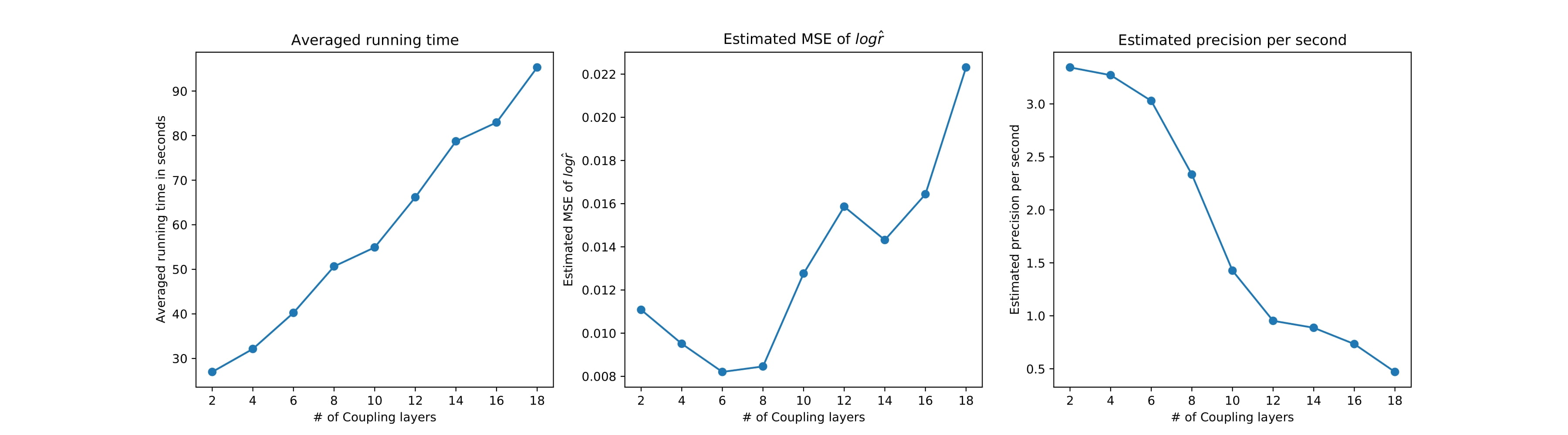
Figure 8: Left: Average running time for each $K$ based on 50 repetitions. Mid: MC estimate of $MSE(\log\hat{r}^{\prime(\phi_{t})}_{opt})$ for each $K$. Right: Estimated precision per second for each $K$.

Splitting the samples from $q_{1},q_{2}$

In Algorithm 2, we first estimate $\{\phi_{t},\tilde{r}_{t}\}$ using the training samples $\{\omega_{ij}\}_{j=1}^{n_{i}}$, then compute the optimal Bridge estimator based on the separate estimating samples $\{\omega^{\prime}_{ij}\}_{j=1}^{n^{\prime}_{i}}$. We use separate samples for the Bridge sampling step because the estimated transformed density $q_{1}^{(\phi_{t})}$ in Algorithm 2 is chosen based on the training samples $\{\omega_{ij}\}_{j=1}^{n_{i}}$ for $i=1,2$. This means the density of the distribution of the transformed training samples $\{T_{\phi_{t}}(\omega_{1j})\}_{j=1}^{n_{1}}$ is no longer proportional to $\tilde{q}_{1}^{(\phi_{t})}(T_{\phi_{t}}(\omega_{1j}))$ for $j=1,...,n_{1}$ as $\phi_{t}$ can be viewed as a function of $\{\omega_{ij}\}_{j=1}^{n_{i}}$. If we apply the iterative procedure (4) to densities $q_{1}^{(\phi_{t})},q_{2}$ and the transformed training samples $\{T_{\phi_{t}}(\omega_{1j})\}_{j=1}^{n_{1}},\{\omega_{2j}\}_{j=1}^{n_{2}}$, then the resulting $\hat{r}_{opt}^{(\phi_{t})}$ will be a biased estimate of $r$. See also Wong et al., (2020) for a detailed discussion under a similar setting. One way to correct this bias is to split the samples from $q_{1},q_{2}$ into training samples $\{\omega_{ij}\}_{j=1}^{n_{i}}$ and estimating samples $\{\omega^{\prime}_{ij}\}_{j=1}^{n^{\prime}_{i}}$ for $i=1,2$. We first estimate the transformation $T_{\phi_{t}}$ using the training samples $\{\omega_{ij}\}_{j=1}^{n_{i}}$, $i=1,2$. Once we have obtained the estimated $\phi_{t}$, we apply the iterative procedure (4) to $\tilde{q}_{1}^{(\phi_{t})},\tilde{q}_{2}$ and the transformed estimating samples $\{T_{\phi_{t}}(\omega^{\prime}_{1j})\}_{j=1}^{n^{\prime}_{1}},\{\omega^{\prime}_{2j}\}_{j=1}^{n^{\prime}_{2}}$, $i=1,2$. Then the resulting estimate $\hat{r}^{\prime(\phi_{t})}_{opt}$ will not suffer from this bias. The same approach is used in Wang et al., (2020) and Jia and Seljak, (2020). The idea of eliminating this bias by splitting the samples from $q_{1},q_{2}$ is further discussed in Wong et al., (2020). The above argument also applies to the estimation of $RE^{2}(\hat{r}^{\prime(\phi_{t})}_{opt})$. We compute $\widehat{RE}^{2}(\hat{r}^{\prime(\phi_{t})}_{opt})$ based on the independent estimating samples using (19). Since finding $\widehat{RE}^{2}(\hat{r}^{\prime(\phi_{t})}_{opt})$ is a 1-d optimization problem, the additional computational cost is negligible compared to the rest of Algorithm 2. In practice, we recommend setting $n_{i}=n^{\prime}_{i}$ for $i=1,2$, i.e. splitting the samples from $q_{1},q_{2}$ into equally sized training samples and estimating samples.

Finding the saddle point using alternating gradient method

In Algorithm 2, we aim to find a saddle point of $L_{\lambda_{1},\lambda_{2}}(\phi,\tilde{r};s_{2},\{\omega_{ij}\}_{j=1}^{n_{i}})$ using the alternating gradient method. This approach is adapted from the Algorithm 1 of Nowozin et al., (2016). The authors show that their Algorithm 1 converges geometrically to a saddle point under suitable conditions. In the alternating training process of Algorithm 2, updating $\tilde{r}_{t+1}$ is a 1-d optimization problem when $\phi_{t}$ is treated as fixed for any step $t$. Hence we can also directly find $\hat{r}_{\phi_{t}}=\operatorname*{arg\,max}_{\tilde{r}\in\mathbb{R}^{+}}L_{\lambda_{1},\lambda_{2}}(\phi_{t},\tilde{r};s_{2},\{\omega_{ij}\}_{j=1}^{n_{i}})$ instead of performing a single step gradient ascent on $\tilde{r}_{t}$. By Proposition 1 and 2, $\hat{r}_{\phi_{t}}$ can be viewed as a (biased) Bridge estimator of $r$ given $\phi_{t}$. However, such estimator $\hat{r}_{\phi_{t}}$ is not reliable when $q_{1}^{(\phi_{t})}$ and $q_{2}$ share little overlap. Therefore directly optimizing $\tilde{r}$ at each iteration $t$ is not always necessary in practice, especially at the early stage of training when $q_{1}^{(\phi_{t})}$ is not yet a sensible approximation of $q_{2}$. In addition, the gradient ascent update of $\tilde{r}_{t}$ is computationally cheaper than finding the optimizer $\hat{r}_{\phi_{t}}$ directly. Therefore we follow Nowozin et al., (2016) and use the alternating gradient method to find the saddle point of $L_{\lambda_{1},\lambda_{2}}(\phi,\tilde{r};s_{2},\{\omega_{ij}\}_{j=1}^{n_{i}})$. We only recommend optimizing $\tilde{r}_{t}$ directly in Algorithm 2 when we know $q_{1}^{(\phi_{t})}$ and $q_{2}$ have at least some degree of overlap.

Note that $\{\phi_{t},\tilde{r}_{t}\}$ being approximately a saddle point of the objective function does not necessarily imply that it solves $\min_{\phi\in\mathbb{R}^{l}}\max_{\tilde{r}\in\mathbb{R}^{+}}L_{\lambda_{1},\lambda_{2}}(\phi,\tilde{r};s_{2},\{\omega_{ij}\}_{j=1}^{n_{i}})$. For $\tilde{r}_{t}$, it is easy to verify if $\tilde{r}_{t}$ is indeed the maximizer of $L_{\lambda_{1},\lambda_{2}}(\phi_{t},\tilde{r};s_{2},\{\omega_{ij}\}_{j=1}^{n_{i}})$ w.r.t. $\tilde{r}\in\mathbb{R}^{+}$ since it is a 1-d optimization problem. However, for $\phi_{t}$ there is no guarantee that it is the global minimizer of $L_{\lambda_{1},\lambda_{2}}(\tilde{r}_{t},\phi;s_{2},\{\omega_{ij}\}_{j=1}^{n_{i}})$ w.r.t. $\phi\in\mathbb{R}^{l}$. One way to address this problem is to run Algorithm 2 multiple times and choose the $q_{1}^{(\phi_{t})}$ that attains the smallest objective function value. In the numerical examples, we find $q_{1}^{(\phi_{t})}$ returned from Algorithm 2 is almost always a good approximation of $q_{2}$. Therefore we do not worry about this problem in practice.

In the alternating training process, seeing the absolute difference between $L_{\lambda_{1},\lambda_{2}}(\phi_{t},\tilde{r}_{t};s_{2},\{\omega_{ij}\}_{j=1}^{n_{i}})$ and $L_{\lambda_{1},\lambda_{2}}(\phi_{t-1},\tilde{r}_{t-1};s_{2},\{\omega_{ij}\}_{j=1}^{n_{i}})$ being less than the tolerance level $\epsilon_{1}$ at an iteration $t$ does not necessarily imply that it has reached a saddle point. Therefore we also need to monitor the sequence $\{\tilde{r}_{t}\}$, $t=0,1,2,...$ in the training process. If $|\tilde{r}_{t}-\tilde{r}_{t-1}|>\epsilon_{2}$, then $\tilde{r}_{t}$ has not converged to a stationary point regardless of the value of the objective function. In other words, we know $\{\phi_{t},\tilde{r}_{t}\}$ has approximately converged to a saddle point only if both the objective function $L_{\lambda_{1},\lambda_{2}}(\phi_{t},\tilde{r}_{t};s_{2},\{\omega_{ij}\}_{j=1}^{n_{i}})$ and $\tilde{r}_{t}$ have stopped changing. In practice, we recommend setting $\epsilon_{1}\in(10^{-3},10^{-1})$ depending on the scale of the objective function, and $\epsilon_{2}\in(10^{-3},10^{-2})$.

Effectiveness of the hybrid objective

As we have discussed previously, we introduce the hybrid objective to stabilize the alternating training process and accelerate the convergence of Algorithm 2. Here we demonstrate the effectiveness of the hybrid objective in Algorithm 2 using the mixture of rings example in Sec 5 with $p=12$, $\boldsymbol{\mu}_{11}=(2,2),\boldsymbol{\mu}_{12}=(-2,-2),\boldsymbol{\mu}_{21}=(2,-2),\boldsymbol{\mu}_{21}=(-2,2)$, $b_{1}=3,b_{2}=6,\sigma_{1}=1,\sigma_{2}=2$. We set $q_{1}^{(\phi)}$ to be a Real-NVP with 5 coupling layers. We first run Algorithm 2 50 times with $n_{i}=n^{\prime}_{i}=1000$ for $i=1,2$ and $\lambda_{1}=\lambda_{2}=0.05$. We record the values of the objective function and $\tilde{r}_{t}$ of the first 25 iterations. Then we run Algorithm 2 50 times with $n_{i}=n^{\prime}_{i}=1000$ for $i=1,2$ and $\lambda_{1}=\lambda_{2}=0$, and record the same values. Recall that setting $\lambda_{1}=\lambda_{2}=0$ is equivalent to using the original $f$-GAN objective (25). From Figure 9 we see most of the hybrid objectives and the corresponding $\tilde{r}_{t}$ values have stabilized after 20 iterations. The stand alone $f$-GAN objective with $\lambda_{1}=\lambda_{2}=0$ also demonstrate a decreasing trend, but the objective values are much more wiggly compared to the hybrid objective due to the adversarial training process, and there is no sign of convergence in 25 iterations. Note that for both the hybrid objective and the original $f$-GAN objective, the corresponding $\tilde{r}_{t}$ tend to converge to a value slightly different from the true $r$ as the number of iteration increases. This is likely due to the bias we discussed previously.

Figure 9: Left: The objective function and $\tilde{r}_{t}$ of the first 25 iterations of Algorithm 2 with $\lambda_{1}=\lambda_{2}=0.05$. Right: The objective function and $\tilde{r}_{t}$ of the first 25 iterations of Algorithm 2 with $\lambda_{1}=\lambda_{2}=0$.

14 Additional simulations

Simulated example: Quantized Mixture of Gaussians

Here we illustrate how Normalizing flows can be used to increase the overlap between discrete random variables in the context of estimating a single normalizing constant (i.e. one of $q_{1},q_{2}$ is completely known). We take the quantized Mixture of Gaussian in Tran et al., (2019) and Metz et al., (2017) as a toy example.

Following Tran et al., (2019), we first define the completely known “base” distribution $q_{1}$. Let $\omega^{(1)},\omega^{(2)}$ be two categorical variables each with 90 states. Let $\omega=(\omega^{(1)},\omega^{(2)})$. Let $q_{1}$ be a uniform distribution over all possible states of $\omega$. The probability mass function of $q_{1}$ is then

$$q_{1}(\omega^{(1)}=u,\omega^{(2)}=v)=\frac{1}{90\times 90}\quad\quad u,v\in\{1,2,...,90\}$$ (71)

We then define the quantized Mixture of Gaussian distribution as our “target” distribution $q_{2}$. In order to define the quantized Mixture of Gaussian, we first define $\tilde{g}(x)$, the unnormalized density of a mixture of 2D Gaussian distributions, to be

$$\tilde{g}(x)=\sum_{k=1}^{K}\pi_{k}\tilde{p}(x;\mu_{k},\sigma^{2}I_{2})$$ (72)

where $x\in\mathbb{R}^{2}$, $I_{2}$ is the $2\times 2$ identity matrix, $\tilde{p}(\cdot;\mu,\Sigma)=\exp(-\frac{1}{2}(x-\mu)^{T}\Sigma^{-1}(x-\mu))$ is the unnormalized 2D Gaussian density with mean $\mu$ and covariance $\Sigma$, $K=4$, $\sigma=0.1$, $\mu_{1}=(2,0)$, $\mu_{2}=(-2,0)$, $\mu_{3}=(0,2)$, $\mu_{4}=(0,-2)$ and $\pi_{k}=\frac{1}{K}$ for $k=1,...,K$. We then truncate the support of $\tilde{g}(x)$ to be $[-2.25,2.25]^{2}$. We now define $q_{2}(\omega)$, the quantized 2D Mixture of Gaussian distribution, by discretizing this square at the 0.05 level (i.e. forming a $90\times 90$ equally spaced grid). This discretization step leads to two categorical variables $\omega^{(1)},\omega^{(2)}$ each with 90 states. For $u,v\in\{1,2,...,90\}$, let $B_{uv}\subseteq[-2.25,2.25]^{2}$ be the cell of the grid that corresponds to the state $\{\omega^{(1)}=u,\omega^{(2)}=v\}$. Then the unnormalized probability mass function of $q_{2}$ can be written as

$$\tilde{q}_{2}(\omega^{(1)}=u,\omega^{(2)}=v)=\int_{x\in B_{uv}}\tilde{g}(x)dx\quad\quad u,v\in\{1,2,...,90\}.$$ (73)

See Figure 11 for a 2D histogram of samples from $q_{2}$. Let

$$Z_{2}=\sum_{u=1}^{90}\sum_{v=1}^{90}\int_{x\in B_{uv}}\tilde{g}(x)dx$$ (74)

be the normalizing constant of $\tilde{q}_{2}(\omega)$, which can be computed easily. Let $q_{2}(\omega)=\tilde{q}_{2}(\omega)/Z_{2}$ be the corresponding normalized pmf. Since $q_{1}$ is completely known, its normalizing constant $Z_{1}$ is equal to $1$ and therefore $\tilde{q}_{1}(\omega)=q_{1}(\omega)$.

Our goal is to estimate $\log r=\log Z_{1}-\log Z_{2}=-\log Z_{2}$ by first increasing the overlap between $q_{1}$ and $q_{2}$ using a Normalizing flow, then compute the asymptotically optimal Bridge estimator of $r$ based of the transformed distributions. Let $N=\{500,1000,1500,2000,2500\}$. To demonstrate the effectiveness of this approach, for each value of $N$, we first draw $n_{1}=n_{2}=N$ training samples $\{\omega_{1j}\}_{j=1}^{n_{1}}$ and $\{\omega_{2j}\}_{j=1}^{n_{2}}$ from $q_{1},q_{2}$ respectively, and use an autoregressive discrete flow Tran et al., (2019) to estimate a bijective transformation $T$ that maps $q_{1}$ to $q_{2}$ based on the training samples and the training procedure given by Tran et al., (2019). One key distinction between discrete flows Tran et al., (2019) and their continuous counterparts (e.g. Dinh et al., (2016); Kingma et al., (2016)) is that for discrete flows, the base distribution $q_{1}$ is treated as a model parameter and is estimated jointly with the transformation $T$. In our example, this means the parameterization (i.e. the $90\times 90$ probability table) we chose for $q_{1}$ in (71) is only treated as the “initial values” of the model parameters, and is updated alongside with the transformation $T$. (Note that when $q_{1},q_{2}$ have a large number of discrete states, storing or updating the probability table of the base $q_{1}$ is computationally infeasible. To alleviate this problem, Tran et al., (2019) also considered more sophisticated parameterizations of the “trainable base” $q_{1}$ such as the autoregressive Categorical distribution.) Let $T_{1}$ be the estimated transformation, $\bar{q}_{1}$ be the updated base distribution (which is also completely known and easy to sample from). Let $\bar{q}_{1}^{(T)}$ be the transformed distribution obtained by applying $T_{1}$ to the samples from the updated $\bar{q}_{1}$. We then draw $n^{\prime}_{1}=n^{\prime}_{2}=N$ estimating samples $\{\bar{\omega}^{\prime}_{1j}\}_{j=1}^{n^{\prime}_{1}}$ and $\{\omega^{\prime}_{2j}\}_{j=1}^{n^{\prime}_{2}}$ from $\bar{q}_{1},q_{2}$ respectively, and compute $\hat{r}^{(T)}_{opt}$ in (7) based on the transformed $\{T_{1}(\bar{\omega}^{\prime}_{1j})\}_{j=1}^{n^{\prime}_{1}}$ and the original $\{\omega^{\prime}_{2j}\}_{j=1}^{n^{\prime}_{2}}$. For each value of $N$, we repeat this process 100 times, and report the MC estimate of $MSE(\hat{r}^{(T)}_{opt})$ based on the repeated $\hat{r}^{(T)}_{opt}$s and the ground truth $r$. Let $\hat{r}_{opt}$ be the optimal Bridge estimator based on the original $\tilde{q}_{1},\tilde{q}_{2}$. For each value of $N$, we compare $MSE(\log\hat{r}^{(T)}_{opt})$ with $MSE(\log\hat{r}_{opt})$, which is also estimated based on 100 repetitions in a similar fashion. From Figure 10 we see $\hat{r}^{(T)}_{opt}$ is a reliable estimator of $r$ for all choice of $N$ and is much more accurate than the optimal Bridge estimator based on the original $\tilde{q}_{1},\tilde{q}_{2}$. From Figure 11 we also see that the transformed $\bar{q}_{1}^{(T)}$ accurately captures the multimodal structure of $q_{2}$.

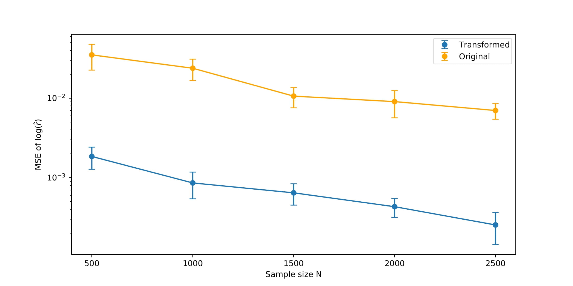
Figure 10: MC estimate of MSE of $\log\hat{r}^{(T)}_{opt}$ and $\log\hat{r}_{opt}$ for each value of $N$. Vertical segments represent the $2\sigma$ error bars.

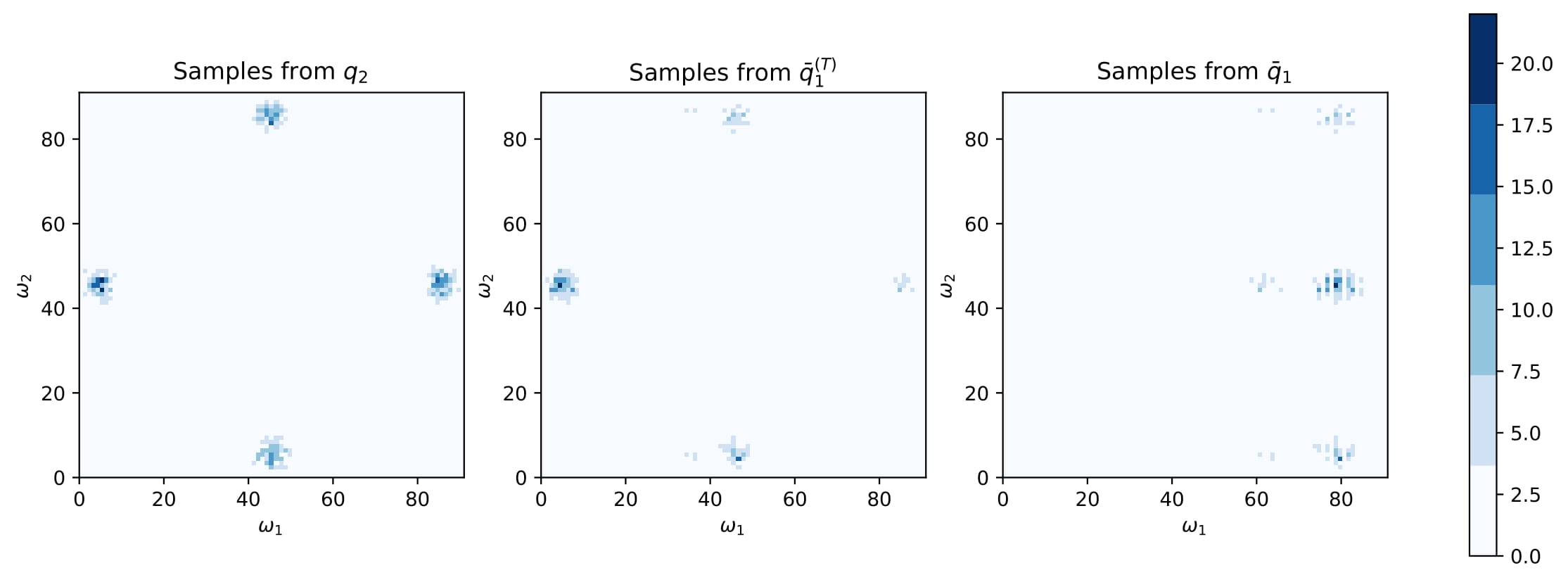
Figure 11: Left: 2D histogram of $10^{3}$ samples from $q_{2}$. Mid: 2D histogram of $10^{3}$ samples from the transformed $\bar{q}_{1}^{(T)}$, which is estimated using $N=10^{3}$ training samples. Right: 2D histogram of $10^{3}$ samples from the corresponding updated base distribution $\bar{q}_{1}$ of the transformed $\bar{q}_{1}^{(T)}$.

In addition to the quantized mixture of Gaussian example, more substantial applications of discrete flows can also be found in Tran et al., (2019). However, the discrete flows in Tran et al., (2019) are in general not directly applicable to our proposed Algorithm 2. This is because in our Algorithm 2, the unnormalized densities $\tilde{q}_{1}$ and $\tilde{q}_{2}$ are specified by the users and therefore can be arbitrary. However, for discrete flows, the “base” distribution has to be completely known, and is treated as a trainable model parameter (as in this example). This means we are not able to use it to directly estimate the ratio of normalizing constants between two arbitrary unnormalized probability mass functions in the same way as in Algorithm 2. Nevertheless, one may obtain an estimator of the ratio of normalizing constants between two discrete distributions by estimating their normalizing constants separately using discrete flows and the procedure used in this example. For future work, we are interested in extending Algorithm 2 so that it is able to handle arbitrary unnormalized pmfs using e.g. more sophisticated Normalizing flow architectures.

Simulated example: Mixture of $t$-distributions

In this example, we let $q_{1}$ and $q_{2}$ be two mixtures of $p$ dimensional $t$-distributions. We are interested in this example because both $q_{1},q_{2}$ are multimodal and have heavy tails. For $i=1,2$, let

$$q_{i}(\omega)=\sum_{k=1}^{K}\pi_{ik}p_{t}(\omega;\mu_{ik},\Sigma_{i},\nu_{i}),$$ (75)

where $K$ is the number of components, $\pi_{i}=\{\pi_{ik}\}_{k=1}^{K}$ are the mixing weights and $p_{t}(\cdot;\mu_{ik},\Sigma_{i},\nu_{i})$, the $k$th component of $q_{i}$ is the pdf of a multivariate $t$-distribution with mean $\mu_{ik}\in\mathbb{R}^{p}$, positive-definite scale matrix $\Sigma_{i}\in\mathbb{R}^{p\times p}$ and degree of freedom $\nu_{i}\in\mathbb{R}^{+}$. Note that all $K$ components of $q_{i}$ have the same covariance structure and degree of freedom. Let

$$Z_{i}=\frac{\Gamma((\nu_{i}+p)/2)}{\Gamma(\nu_{i}/2)\nu_{i}^{p/2}\pi^{p/2}|\Sigma_{i}|^{1/2}}$$ (76)

be the normalizing constant of $p_{t}(\cdot;\mu_{ik},\Sigma_{i},\nu_{i})$. Note that this quantity does not depend on $\mu_{ik}$. Let $\tilde{p}_{t}(\cdot;\mu_{ik},\Sigma_{i},\nu_{i})=Z_{i}p_{t}(\cdot;\mu_{ik},\Sigma_{i},\nu_{i})$ be the unnormalized density of each component $p_{t}(\cdot;\mu_{ik},\Sigma_{i},\nu_{i})$. Let $\tilde{q}_{i}(\omega)=\sum_{k=1}^{K}\pi_{ik}\tilde{p}_{t}(\omega;\mu_{ik},\Sigma_{i},\nu_{i})$ be the unnormalized density of $q_{i}(\omega)$. It is easy to verify that $\tilde{q}_{i}(\omega)=Z_{i}q_{i}(\omega)$, i.e. the normalizing constant of $\tilde{q}_{i}(\omega)$ is $Z_{i}$.

For this example, we consider $p=\{5,10,20,40,60,80,100\}$. For each choice of $p$, the parameters of $q_{1},q_{2}$ are chosen in the following way: We fix the degree of freedom $\nu_{1}=1,\nu_{2}=4$, and number of component $K=7$. The mixing weights $\pi_{i}$ for $i=1,2$ are sampled independently from a $Dir(\alpha_{1},...,\alpha_{K})$ where $\alpha_{k}=1$ for $k=1,...,K$. The location parameters $\mu_{ik}$ for $i=1,2$, $k=1,...,K$ are sampled from a standard Normal $N(0,I_{p})$ independently. For the scale matrices $\Sigma_{i}$, we first sample $\Sigma_{1},\Sigma_{2}$ independently from a inverse Wishart distribution $\mathcal{W}^{-1}(I_{p},p)$, then rescale $\Sigma_{1},\Sigma_{2}$ so that $\left|\Sigma_{1}\right|=1$ and $\left|\Sigma_{2}\right|\ =1000$. This ensures the components of $q_{1}$ are more concentrated than the components in $q_{2}$.

We estimate $\log r=\log Z_{1}-\log Z_{2}$ in a similar fashion to the previous examples. For each choice of $p$, we run each method 30 times. Let $\hat{r}$ be a generic estimate of $r$. We use the MC estimate of RMSE of $\log\hat{r}$, i.e. $E((\log\hat{r}-r)^{2})/(\log r)^{2}$, based on the repeated runs as the benchmark of performance for this example. For each repetition, we run each method with $N_{1}=N_{2}=6000$ independent samples from $q_{1},q_{2}$ respectively. For our Algorithm 2, we parameterize $q_{1}^{(\phi)}$ as a Real-NVP with 20 coupling layers, and set $\lambda_{1}=\lambda_{2}=0.01$. For the rest of the methods, we use the deafult or recommended settings. The results are summarized in Table 1. We see our Algorithm 2 outperforms all methods when $p\geq 40$.

$p$	$f$-GAN	GBS	Warp-III	Warp-U
$5$	3.69e-5	8.22e-4	1.14e-3	3.54e-5
$10$	6.21e-5	1.74e-3	5.15e-3	6.42e-5
$20$	4.12e-3	4.96e-3	8.87e-3	1.69e-3
$40$	1.23e-2	4.05e-2	9.01e-2	5.75e-2
$60$	1.21e-2	3.88e-2	9.26e-2	7.64e-2
$80$	1.81e-2	5.20e-2	1.59e-1	6.05e-2
$100$	2.46e-2	8.14e-2	-	4.78e-1

Table 1: The estimated RMSE of the $\log\hat{r}$ of each methods based on 30 repeated runs. The lowest estimated RMSE for each $p$ is in boldface. Warp-III does not converge for most of the repeated runs when $p=100$ so we are not able to estimate its RMSE.

15 Computational cost of Algorithm 2

Comparing the computational cost of our Algorithm 2 with existing methods and their existing implementations is not straightforward because of the very different nature of GPU and CPU computing. In both examples, we compare the existing CPU implementations of Warp-III, Warp-U, GBS and a GPU implementation of our Algorithm 2 in term of wall clock time. We think this comparison is not unfair because there is no simple way to accelerate existing algorithms with a GPU, while training neural nets on GPU was a design element in implementing Algorithm 2 using deep learning frameworks such as Torch (Paszke et al.,, 2017). If a user have access to both CPU and GPU, then we believe the wall clock time to some extent can be viewed as a natural metric of the time cost a user has to pay for the estimator. And the Precision per Second benchmark can be viewed as the cost-performance ratio of these methods. This measure is not a rigorous metric for comparing computation costs, but we believe it is at least an intuitive one for the users to get a rough idea of the time cost and efficiency of these algorithms.

From the numerical examples we see $f$-GB scaled better with dimension than its competitors. For example, from Example 1 we see that even though Warp-III can be $30\sim 40$ faster to compute than our proposed method given the same amount of samples from $q_{1},q_{2}$, its accuracy (measured in $MSE(\log\hat{r})$) is orders of magnitude greater (worse) than our approach. When $p=48$, we find that Warp-III is not able to return a sensible estimate of $r$ even with 25 times more samples from $q_{1},q_{2}$ than $f$-GB. In Example 2 we also find that Warp-III requires around 18 times more samples to achieve a similar level of accuracy as $f$-GB, and takes around 3 times longer to run. Therefore we believe the extra computational cost of our $f$-GB estimator is “well-spent” as the numerical examples show that our Algorithm 2 is able to return an estimate of $r$ with much higher precision than GBS, Warp-III and Warp-U and scales better with the dimension of the distributions.

As we acknowledge in Sec 7, if $q_{1},q_{2}$ are simple structured and low dimensional, then users can get adequate precision more quickly using Warp-III or Warp-U. On the other hand, in speaking to users who report Bayes factors in applied Bayesian work, the overwhelming requirement was that the estimate be reliable, as the Bayes Factor value is sometimes the crux. In all the numerical examples we considered, $f$-GB never broke and produced accurate estimates. Warp III and GBS did break on larger problems. Warp-U took a similar amount of time to run compared with $f$-GB, but was less accurate. Therefore users may still prefer a method which is “over-powered” but more reliable.

References

- Ali and Silvey, (1966) Ali, S. M. and Silvey, S. D. (1966). A general class of coefficients of divergence of one distribution from another. Journal of the Royal Statistical Society: Series B (Methodological), 28(1):131–142.
- Arjovsky and Bottou, (2017) Arjovsky, M. and Bottou, L. (2017). Towards principled methods for training generative adversarial networks. arXiv preprint arXiv:1701.04862.
- Bennett, (1976) Bennett, C. H. (1976). Efficient estimation of free energy differences from monte carlo data. Journal of Computational Physics, 22(2):245–268.
- Bridges et al., (2009) Bridges, M., Feroz, F., Hobson, M., and Lasenby, A. (2009). Bayesian optimal reconstruction of the primordial power spectrum. Monthly Notices of the Royal Astronomical Society, 400(2):1075–1084.
- Burda et al., (2015) Burda, Y., Grosse, R., and Salakhutdinov, R. (2015). Accurate and conservative estimates of mrf log-likelihood using reverse annealing. In Artificial Intelligence and Statistics, pages 102–110. PMLR.
- Chen and Shao, (1997) Chen, M.-H. and Shao, Q.-M. (1997). Estimating ratios of normalizing constants for densities with different dimensions. Statistica Sinica, pages 607–630.
- Creswell et al., (2018) Creswell, A., White, T., Dumoulin, V., Arulkumaran, K., Sengupta, B., and Bharath, A. A. (2018). Generative adversarial networks: An overview. IEEE Signal Processing Magazine, 35(1):53–65.
- Dinh et al., (2016) Dinh, L., Sohl-Dickstein, J., and Bengio, S. (2016). Density estimation using real nvp. arXiv preprint arXiv:1605.08803.
- Durkan et al., (2019) Durkan, C., Bekasov, A., Murray, I., and Papamakarios, G. (2019). Neural spline flows. arXiv preprint arXiv:1906.04032.
- Fitzmaurice and Laird, (1993) Fitzmaurice, G. M. and Laird, N. M. (1993). A likelihood-based method for analysing longitudinal binary responses. Biometrika, 80(1):141–151.
- Fourment et al., (2020) Fourment, M., Magee, A. F., Whidden, C., Bilge, A., Matsen IV, F. A., and Minin, V. N. (2020). 19 dubious ways to compute the marginal likelihood of a phylogenetic tree topology. Systematic biology, 69(2):209–220.
- Friel and Wyse, (2012) Friel, N. and Wyse, J. (2012). Estimating the evidence–a review. Statistica Neerlandica, 66(3):288–308.