Machine Learning Implicit Solvation for Molecular Dynamics

Abstract

Accurate modeling of the solvent environment for biological molecules is crucial for computational biology and drug design. A popular approach to achieve long simulation time scales for large system sizes is to incorporate the effect of the solvent in a mean-field fashion with implicit solvent models. However, a challenge with existing implicit solvent models is that they often lack accuracy or certain physical properties compared to explicit solvent models, as the many-body effects of the neglected solvent molecules is difficult to model as a mean field. Here, we leverage machine learning (ML) and multi-scale coarse graining (CG) in order to learn implicit solvent models that can approximate the energetic and thermodynamic properties of a given explicit solvent model with arbitrary accuracy, given enough training data. Following the previous ML–CG models CGnet and CGSchnet, we introduce ISSNet, a graph neural network, to model the implicit solvent potential of mean force. ISSNet can learn from explicit solvent simulation data and be readily applied to MD simulations. We compare the solute conformational distributions under different solvation treatments for two peptide systems. The results indicate that ISSNet models can outperform widely-used generalized Born and surface area models in reproducing the thermodynamics of small protein systems with respect to explicit solvent. The success of this novel method demonstrates the potential benefit of applying machine learning methods in accurate modeling of solvent effects for in silico research and biomedical applications.

I Introduction

The solvent environment around macromolecules often plays a significant, sometimes even decisive, role in both the structure and dynamics of biological systems.(Laage, Elsaesser, and Hynes, 2017; Lewandowski et al., 2015; Daniel, Finney, and Stoneham, 2004) For example, the so-called “hydrophobic core”, a key structural element shared by a diverse variety of protein domains strongly influences protein folding in aqueous solution.(Ball, 2008; Kalinowska et al., 2017) The solvent also renders the protein structure flexible enough for functional conformational changes (Barron, Hecht, and Wilson, 1997) and mediates interactions among macromolecules for biological processes (Ball, 2008; Levy and Onuchic, 2006) as well as drug binding.Ben-Naim, 2002; Persch, Dumele, and Diederich, 2015; Ladbury, 1996

Thus, for computational investigations of biomedical problems, such as molecular dynamics (MD) simulations of biological systems Adcock and McCammon, 2006; Dror et al., 2012; Braun et al., 2018 and molecular docking,(Brooijmans and Kuntz, 2003) we often seek to accurately model effects of the solvent environment. In MD simulations, solvation methods can be grouped into two major categories: explicit and implicit. The former—as illustrated in Fig. 1a—incorporates solvent molecules explicitly into the simulation system, while the latter (see Fig. 1b) represents solvent effects in a mean-field manner.(Adcock and McCammon, 2006; Onufriev and Izadi, 2018; Ren et al., 2012) Treating the solvent implicitly has several advantages: it can speed up force calculations by drastically reducing the the number of degrees of freedom; it increases the effective time step size in MD simulations;(Anandakrishnan et al., 2015) and it simplifies constant-pH simulations (Baptista, Teixeira, and Soares, 2002; Mongan, Case, and McCammon, 2004) as well as enhanced sampling approaches, such as parallel tempering (PT)/replica-exchange MD.(Trebst, Troyer, and Hansmann, 2006; Earl and Deem, 2005) Moreover, implicit solvent treatment is very common in structure-based drug design, such as fragment screening and lead optimization.Śledź and Caflisch, 2018; Wang et al., 2019a Some generalized Born (GB)-based implicit solvent methods, for example, are implemented in various MD software packages, such as GBSA–HCT,(Hawkins, Cramer, and Truhlar, 1996) GBSA–OBC and GBn models (Roe et al., 2007) in AMBER,(Amb, ) GBMV (Lee, Salsbury Jr, and Brooks III, 2002; Lee et al., 2003) and GBSW models (Im, Lee, and Brooks III, 2003) in CHARMM.(Brooks et al., 2009) Ref. Knight and Brooks III, 2011 gives an comprehensive comparison of available implicit solvent models.

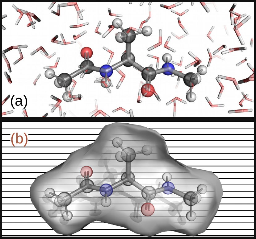
Figure 1: (a) Explicit and (b) implicit solvation treatment of a biomolecular system (here we use capped alanine as an example).

Despite their advantages, the accuracy of commonly used implicit solvent models tends to be inadequate in certain applications, such as the calculation of solvation free energies (Cumberworth, Bui, and Gsponer, 2016) or the recovery of correct conformational distributions for folded and unfolded states of proteins,(Zhou and Berne, 2002; Nymeyer and Garcia, 2003; Zhou, 2003) thereby limiting their usage and effectiveness in practice.

The present work addresses a long-standing question in solvent modeling: is it possible to construct mean-field implicit solvent models that reproduce the solvation thermodynamics of explicit-solvent systems exactly? We approach this problem by parameterizing implicit solvent models via a machine-learned coarse graining approach. Coarse graining of molecular systems is itself a well-researched topic, one whose aim is to model molecules and their interactions with super-atomistic resolutions, such that computational investigations (e.g., MD simulations) become more efficient.(Clementi, Nymeyer, and Onuchic, 2000; Clementi, 2008; Saunders and Voth, 2013; Noid, 2013; Ingólfsson et al., 2014; Kmiecik et al., 2016; Pak and Voth, 2018; Chen et al., 2018; Singh and Li, 2019; Nüske, Boninsegna, and Clementi, 2019; Wang et al., 2019b, 2020; Husic et al., 2020) A coarse grained (CG) model usually entails two important aspects: the CG resolution and representation—that is, the mapping of the original atoms into effective interacting groups (also known as CG beads) (Kmiecik et al., 2016; Pak and Voth, 2018; Noid, 2013; Farrell, Oden, and Faghihi, 2015; Boninsegna, Banisch, and Clementi, 2018)—and the CG potential, which determines the interactions among the CG beads.(Pak and Voth, 2018; Noid, 2013; Kmiecik et al., 2016) Here we consider an implicit solvent system as a CG version of the explicit solvent system—the CG mapping keeps the solute molecule(s) while removing the solvent degrees of freedom. Once the CG mapping has been assigned, the parameterization of a CG potential may follow either a “top-down” approach; i.e., one that aims at reproducing macroscopic experimental observations, or a “bottom-up” strategy, which systematically integrates information from the corresponding atomistic system.(Noid, 2013) In this work we leverage the multi-scale coarse graining theory,(Izvekov and Voth, 2005; Noid et al., 2008a) a “bottom-up” approach. Essentially, it transforms the parameterization of a CG potential into a data-driven optimization based on the variational force matching (FM) method.

The multi-scale coarse graining theory enables us to employ a machine learning method similar to the CGnet introduced by Wang et al. (Wang et al., 2019b) to learn an implicit solvent model, which is part of the CG potential for the solute, for any given molecular system. Machine learning methods have enjoyed increased in popularity and led to breakthroughs in many fields,(LeCun, Bengio, and Hinton, 2015) including molecular sciences.(Butler et al., 2018; Noé et al., 2020; Behler, 2016; Chmiela et al., 2018) For structural coarse graining in particular, there have been some pioneering works both for choosing optimal CG mappings (Wang and Gómez-Bombarelli, 2019; Boninsegna, Banisch, and Clementi, 2018) and for parameterizing CG potentials for a given system.(Zhang et al., 2018; Wang et al., 2019b; Husic et al., 2020; Wang and Gómez-Bombarelli, 2019; Wang et al., 2021) In this work, we adapt the architecture of CGnet (Wang et al., 2019b) and its extension CGSchNet (Husic et al., 2020) (the latter based on a graph neural network architecture SchNet (Schütt et al., 2018)) to the implicit solvent problem. The resulting implicit-solvent SchNet—henceforth called ISSNet—is able to learn an implicit solvent model from coordinate and force samples of a corresponding explicit solvent system. Trained ISSNet models can in turn be used for implicit solvent simulations of biomolecules.

Recently, machine learning methods have been applied in some studies related to solvent environment, such as the automatable cluster-continuum modeling of the solvent in quantum chemistry calculations,(Basdogan et al., 2019) for the parameterization of CG water models for ice-water mixture (Chan et al., 2019) and liquid water systems,(Patra et al., 2019) and for the computation of generalized Born radii in implicit solvent simulations.(Mahmoud et al., 2020) The latter three studies are applicable to MD simulations; however, the goal is either to achieve higher accuracy for water-only systems or to improve the efficiency of an existing method. This work distinguishes itself from existing studies by introducing a neural-network-based implicit solvent method for biomolecular MD simulations. Additionally, we are aware of an interesting study which also integrated variational coarse graining theories to the optimization of an implicit solvent model. (Bottaro, Lindorff-Larsen, and Best, 2013) However, different from the relative entropy method used by their work, the multiscale coarse graining formalism enables simultaneous optimization of all parameters in a complex neural network model without the necessity of iterative sampling.

The paper proceeds as follows: we first describe the theoretical basis of implicit solvent treatment with ISSNet as well as the implementation, including the neural network architecture, training and validation as well as implicit solvent simulation. In the Results we apply our proposed method to two molecular systems—capped alanine (i.e., the solute molecule in Fig. 1) and the miniprotein chignolin.(Honda et al., 2008) We show that our method can reproduce the solvated thermodynamics with higher accuracy than a reference implicit solvent method, namely the GBSA–OBC model.(Onufriev, Bashford, and Case, 2004) In the Discussion section we address the current limitation and future investigative directions of the ISSNet method.

II Theory and Methods

Here, we introduce the potential of mean force (PMF)—a concept from statistical mechanics—as a theoretical basis both for implicit solvent methods and for the multi-scale coarse graining theory. After examining how a traditional approach approximates the implicit solvent PMF, we adapt an established machine learning CG method for parameterizing implicit solvent models based on explicit solvent simulation data.

II.1 Solute PMF and solvation free energy

The concept of PMF originated in a 1935 paper by J. G. Kirkwood on statistical treatment of fluid mixtures.(Kirkwood, 1935) In this subsection we derive the expression of a solute PMF following the framework of Ref. Roux and Simonson, 1999.

Suppose we have an explicit solvent all-atom molecular system with a total number of $N$ atoms, consisting of $N_{mol}$ solute atoms with coordinates $\mathbf{r}$ (e.g., biomolecule) and $(N-N_{mol})$ solvent atoms with coordinates $\mathbf{w}$ (e.g., water atoms and ions). Usually, an all-atom molecular mechanics force field, such as AMBER (Amb, ) or CHARMM,(Brooks et al., 2009) formulates a molecular potential function $v(\mathbf{r},\mathbf{w})$ as a sum of bonded and non-bonded terms.(Adcock and McCammon, 2006; Braun et al., 2018) Therefore, without loss of generality, we can decompose $v(\mathbf{r},\mathbf{w})$ into three partial sums:(Roux and Simonson, 1999) $v_{mol}(\mathbf{r})$ for interactions solely within and between the solute molecule(s), $v_{w}(\mathbf{w})$ for those solely within and between solvent molecules and $v_{mw}(\mathbf{r},\mathbf{w})$ for solute-solvent interactions:

$$v(\mathbf{r},\mathbf{w})=v_{mol}(\mathbf{r})+v_{w}(\mathbf{w})+v_{mw}(\mathbf{r},\mathbf{w}).$$ (1)

We will refer to the solute-only potential $v_{mol}(\mathbf{r})$ as the “vacuum potential”, since it only consists of terms that describe the solute molecule(s) in vacuum.

For a chosen thermodynamic state (e.g., with fixed number of atoms $N$, volume $V$ and temperature $T$ in a canonical ensemble), the equilibrium probability density $p(\mathbf{r},\mathbf{w})$ for a solute-solvent configuration $\mathbf{r},\mathbf{w}$ is:

$$p(\mathbf{r},\mathbf{w})=\frac{\mathrm{e}^{-\beta v(\mathbf{r},\mathbf{w})}}{\int\mathrm{d}\mathbf{r}\int\mathrm{d}\mathbf{w}\>\mathrm{e}^{-\beta v(\mathbf{r},\mathbf{w})}},$$ (2)

where the scaling factor $\beta$ depends on the thermodynamic ensemble used. In the canonical (NVT) ensemble at temperature $T$ it is given by $\beta:=1/(k_{B}T)$ with Boltzmann constant $k_{B}$. The distribution $p(\mathbf{r},\mathbf{w})$ can be sampled as a whole by MD or Monte Carlo simulations with the explicit solvent potential $v(\mathbf{r},\mathbf{w})$.

For implicit solvent models, we are interested in recovering a potential that describes the distribution of the solute molecules only. The density associated with this potential is formed as the marginal density obtained by integrating over the solvent degrees of freedom:

$$P(\mathbf{r}):=\int\mathrm{d}\mathbf{w}\>p(\mathbf{r},\mathbf{w}).$$ (3)

We seek a potential function of solute coordinates $V(\mathbf{r})$ that could generate the marginal distribution $P(\mathbf{r})$. In other words, the potential $V(\mathbf{r})$ should satisfy the following equation:

$$\frac{\mathrm{e}^{-\beta V(\mathbf{r})}}{\int\mathrm{d}\mathbf{r}\>\mathrm{e}^{-\beta V(\mathbf{r})}}=P(\mathbf{r}).$$ (4)

By inserting Eq. (2) and (3) and solving for $V(\mathbf{r})$, we have

$$V(\mathbf{r})=-\beta^{-1}\ln\left[\int\mathrm{d}\mathbf{w}\>\mathrm{e}^{-\beta v(\mathbf{r},\mathbf{w})}\right]+\textrm{const}.$$ (5)

$V(\mathbf{r})$ is the so-called solute PMF,(Roux and Simonson, 1999; Kirkwood, 1935) because its force corresponds to the mean force on the solute coordinates:

$$\mathbf{F}(\mathbf{r}):=-\nabla_{\mathbf{r}}V(\mathbf{r})=\left\langle\mathbf{f_{\mathbf{r}}}(\mathbf{r},\mathbf{w})\right\rangle_{\mathbf{r}},$$ (6)

where

$$\mathbf{f}_{\mathbf{r}}(\mathbf{r,\mathbf{w}}):=\left[-\frac{\partial v}{\partial\mathbf{r}_{1}},\cdots,-\frac{\partial v}{\partial\mathbf{r}_{N}}\right]^{T}$$ (7)

denotes the forces on solute coordinates $\mathbf{r}$ with the solvent conformation being $\mathbf{w}$, and

$$\left\langle\cdot\right\rangle_{\mathbf{r}}:=\int\mathrm{d}\mathbf{w}\>\cdot p(\mathbf{r},\mathbf{w})$$

is a marginal operator that averages over all solvent configurations consistent with a given solute configuration according to the Boltzmann distribution $p(\mathbf{r},\mathbf{w})$.

Theoretically, if we have $V(\mathbf{r})$ as defined in Eq. (5) in the first place, then we can directly sample $P(\mathbf{r})$ as in Eq. (3) and analyze most biologically relevant processes, where solvent coordinates can be ignored (e.g., protein folding, protein-ligand binding or in general any observable defined by a function of the solute conformations only).(Roux and Simonson, 1999) However, in most cases we cannot solve the integral in Eq. (5) analytically.

Alternatively, one can try to construct an approximation to the exact PMF, which is usually determined by first fixing a range of candidates with fixed functional forms $\{V(\mathbf{r};\Theta)\}$ and then optimizing the parameter $\Theta$. An often adopted decomposition in the parameterization is to separate the vacuum potential from the solvent-solvent and the solute-solvent interactions. Applying Eq. (1) to Eq. (5), we can move $v_{mol}(\mathbf{r})$ out of the integral and thus

$$V(\mathbf{r})=v_{mol}(\mathbf{r})+V_{solv}(\mathbf{r}),$$ (8)

in which the solvation free energy $V_{solv}$ is defined as a function of solute configuration

$$V_{solv}(\mathbf{r}):=-\beta^{-1}\ln\left[\int\mathrm{d}\mathbf{w}\>\mathrm{e}^{-\beta\left[v_{w}(\mathbf{w})+v_{mw}(\mathbf{r},\mathbf{w})\right]}\right]+\textrm{const}.$$ (9)

Since the vacuum potential $v_{mol}(\mathbf{r})$ is known a priori from the all-atom force field, we can write any candidate for approximating the solute PMF $V(\mathbf{r})$ in the following form:

$$V(\mathbf{r};\Theta):=v_{mol}(\mathbf{r})+V_{solv}(\mathbf{r};\Theta),$$ (10)

and optimizing $V(\mathbf{r};\Theta)$ is equivalent to finding the best approximation $V_{solv}(\mathbf{r};\Theta^{*})$ to the solvation free energy as defined in Eq. (9). $V_{solv}(\mathbf{r};\Theta^{*})$ is an implicit solvent model, since it does not explicitly involve any solvent, but can be used to approximately sample the Boltzmann distribution of solute conformations by taking into account the solvent environment implicitly according to Eq. (4).

II.2 Traditional implicit solvent models

A widely used strategy for parameterizing implicit solvent models is to decompose the solvation free energy (Eq. (9)) into two terms: the non-polar $V_{solv}^{\textrm{np}}$ and the electrostatic (polar) $V_{solv}^{\textrm{elec}}$ contributions

$$V_{solv}(\mathbf{r})=V_{solv}^{\textrm{np}}(\mathbf{r})+V_{solv}^{\textrm{elec}}(\mathbf{r}),$$ (11)

and seek approximations for both terms separately (details can be found in Ref. Roux and Simonson, 1999). Various models have been developed based on generalization of simple physical models and/or heuristics (Chen, Brooks, and Khandogin, 2008; Feig, Tanizaki, and Sayadi, 2008; Kleinjung and Fraternali, 2014) for each of the two terms.

Here we illustrate Eq. (11) through an example of the popular generalized Born models.(Chen, Brooks, and Khandogin, 2008; Feig, Tanizaki, and Sayadi, 2008; Kleinjung and Fraternali, 2014) As the name suggests, these models employ an approximation to the electrostatics by generalizing the Born model (Born, 1920) for charged spherical particles (e.g., simple ions):

$$V_{solv,\textrm{GB}}^{\textrm{elec}} =\frac{1}{2}\left(\frac{1}{\epsilon_{out}}-\frac{1}{\epsilon_{in}}\right)\sum_{i,j}\frac{q_{i}q_{j}}{f_{ij}},$$ (12a)

$$\textrm{in which }f_{ij} =\sqrt{r_{ij}^{2}+B_{i}B_{j}\exp\left(-\frac{r_{ij}}{4B_{i}B_{j}}\right)},$$ (12b)

where $\epsilon_{out}$ and $\epsilon_{in}$ are outer and inner (regarding the generalized Born sphere) dielectric constants, respectively. Parameters $\left\{q_{i}\right\}$, $\left\{r_{ij}\right\}$ and $\left\{B_{i}\right\}$ denote the atomic partial charges, the pairwise distances and the generalized Born radii, respectively.(Onufriev and Case, 2019; Tsui and Case, 2000) The non-polar contributions are typically represented by a linear function of the solvent-accessible surface area (SASA) is used to represent the non-polar term

$$V_{solv,\textrm{SA}}^{\textrm{np}}=\gamma A(\mathbf{r})\;(+V_{0}^{\textrm{np}}),$$ (13)

in which $\gamma$ is a model parameter with the unit of surface tension and $A(\mathbf{r})$ denotes the surface area associated with the solute configuration $\mathbf{r}$ (sometimes a predetermined offset $V_{0}^{\textrm{np}}$ is also used).(Qiu et al., 1997; Levy et al., 2003) Generalized Born models together with a SASA-based non-polar treatment form the so-called GBSA models, although other variants of non-polar terms also exist.(Roux and Simonson, 1999; Onufriev and Case, 2019) Reference Onufriev and Case, 2019 provides a useful review for the development and commonly used variants of generalized Born models.

II.3 Implicit solvent model from a coarse-graining point of view

We put forward an alternative way for finding an approximation to the solute PMF (Eq. (4)) by adapting the multi-scale coarse graining theory, which enables us to directly optimize a candidate implicit solvent model against the conformations and corresponding forces from explicit solvent simulations. Similar ideas have been successfully applied to models of lipid bilayers (Izvekov and Voth, 2009) and ionic solutions (Cao et al., 2013) under the name of solvent-free coarse graining, but not to complex polymer systems, such as peptide and proteins.

The multi-scale coarse graining theory was developed for parameterizing potential functions for a CG system obtained through a linear CG mapping that satisfies some general requirements (e.g., one atom cannot be assigned to more than one CG bead).(Izvekov and Voth, 2005; Noid et al., 2008a) Since detailed derivations can be found in Ref. Noid et al., 2008a, here we focus on its implications for the implicit solvation problem.

Consider a CG mapping $\Xi$ that treats each solute atom in a system as a “CG particle”:

$$\mathbf{r}=\Xi\mathbf{\left[\begin{array}[]{c}\mathbf{r}\\ \mathbf{w}\end{array}\right]},\;\Xi=\mathbf{\left[\begin{array}[]{c}\mathbf{I}_{\mathrm{N_{mol}}}\\ \mathbf{0}\end{array}\right]},$$ (14)

where this linear transformation essentially truncates the coordinates by eliminating the solvent degrees of freedom. It is straightforward to show that the CG system defined by the mapping $\Xi$ can be treated under the multi-scale coarse graining framework, and the solute PMF defined by Eq. (4) is a CG PMF with thermodynamic consistency.(Noid et al., 2008a) Moreover, the mean force, $\mathbf{F}(\mathbf{r})$, acting on the solute (as derived in Eq. (6)) is a CG mean force.

More than merely a change of notation, treating the implicit solvent system as a CG system of the explicit one enables us to apply the variational FM method for parameterizing an implicit solvent model. For each candidate potential function $V(\mathbf{r};\Theta)$, the multi-scale coarse graining functional (Noid et al., 2008a) is defined as:

$$\chi\left[\Theta\right]:=\frac{1}{3N_{mol}}\left\langle\left\|\mathbf{f}_{\mathbf{r}}(\mathbf{r})+\nabla_{\mathbf{r}}V\left(\mathbf{r};\Theta\right)\right\|^{2}\right\rangle,$$ (15)

where $\mathbf{f}_{\mathbf{r}}$ is defined in Eq. (7), $\left\|\cdot\right\|$ is the Frobenius norm and the bracket $\left\langle\cdot\right\rangle$ indicates an average over a Boltzmann distribution of fine grained configurations $(\mathbf{r},\mathbf{w})$. The multi-scale coarse graining theory states that the global minimum of this functional is unique (up to a constant) and corresponds to the CG PMF $V(\mathbf{r})$, when the space of all possible functions is considered.(Noid et al., 2008a) Furthermore, within a given family of functions parameterized as $\{V(\mathbf{r};\Theta)\}$, one can variationally optimize the approximation by minimizing $\chi\left[\Theta\right]$.

Specifically for an implicit solvent model $V_{solv}(\mathbf{r};\Theta)$, the multi-scale coarse graining functional can be rewritten into the following form (implicit solvent functional) with the vacuum force $\mathbf{f}_{mol}(\mathbf{r})=-\nabla_{\mathbf{r}}U_{mol}$:

$$\chi\left[\Theta\right]=\frac{1}{3N_{mol}}\left\langle\left\|\mathbf{f}_{\mathbf{r}}-\mathbf{f}_{mol}+\nabla_{\mathbf{r}}V_{solv}\left(\mathbf{r};\Theta\right)\right\|^{2}\right\rangle.$$ (16)

II.4 Machine learning of a CG model and of an implicit solvent model

Consider the parameterization of a CG force field: we usually choose a specific form of potential energy functions $\{V(\mathbf{r};\Theta)\}$ with trainable parameters $\Theta$, and then try to assign suitable parameters $\Theta^{*}$, such that the model acquires desired accuracy for representing the system of interest. The function form can be either simple (e.g., Go-models) or complex (e.g., expressed by neural networks). The performance assessment, i.e., the criteria for a good model, can vary depending on the actual problem. However, after we fix the functional form and the criterion (or a finite set of criteria) to assess the “suitability” of a given model, the parameterization procedure fits into the category of supervised machine learning. In other words, we can approximate the CG PMF by numerically optimize the trainable parameters $\Theta$.

In the context of multi-scale coarse graining, the criterion is the functional defined in Eq. (15). Although its value usually cannot be directly computed analytically, we can use a data-driven approximation in the minimization procedure:

$$\chi\left[\Theta\right]\approx L\left[\{\mathbf{r}_{i}\},\{\mathbf{f}_{i}\};\Theta\right]=\frac{1}{3NM}\sum_{i=1}^{M}\left\|\mathbf{f}_{i}+\nabla_{\mathbf{r}}V\left(\mathbf{r}_{i};\Theta\right)\right\|^{2},$$ (17)

which averages over a batch of CG coordinates $\{\mathbf{r}_{i}\}$ ($M$ frames) and corresponding instantaneous forces $\{\mathbf{f}_{i}\}$ after CG mapping sampled from the thermodynamic equilibrium of the fine-grained system. $L\left[\{\mathbf{r}_{i}\},\{\mathbf{f}_{i}\};\Theta\right]$ in Eq. (17) is often referred to as CG–FM error due to its mean-squared-difference form,(Noid et al., 2008a, b) and may serve as a loss function in the numerical optimization of $\Theta$.

The CGnet method,(Wang et al., 2019b) for example, expresses the candidate CG potential as an artificial neural network based on molecular features, such as pairwise distances, the angles and dihedral angles formed by the CG particles. Since this potential is fully determined by the neural network parameters, the optimization of candidate function is equivalent to standard neural network training in a supervised learning problem. Within this general framework, an improved version—CGSchNet—has been developed by using a more sophisticated graph neural network instead of multi-layer perceptrons (see the next subsection for details).(Husic et al., 2020)

Similarly, from the implicit solvent functional (Eq. (16)) we can construct the implicit solvent FM loss function:

$$L\left[\{\mathbf{r}_{i}\},\{\mathbf{f}_{i}\};\Theta\right]=\\ \frac{1}{3NM}\sum_{i=1}^{M}\left\|\mathbf{f}_{i}-\mathbf{f}_{mol}\left(\mathbf{r}_{i}\right)+\nabla_{\mathbf{r}}V_{solv}\left(\mathbf{r}_{i};\Theta\right)\right\|^{2},$$ (18)

where the $\{\mathbf{r}_{i}\}$ and $\{\mathbf{f}_{i}\}$ are coordinates and forces for the solute from an equilibrated explicit solvent sample, and $\mathbf{f}_{mol}$ for the vacuum force as defined in Eq. (16). An implicit solvent potential $V_{solv}\left(\mathbf{r}_{i};\Theta\right)$ can thus be learned for a given molecular system using a given optimizable model (e.g., a neural network).

II.5 The ISSNet architecture

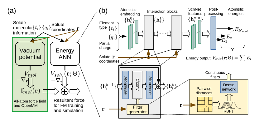
Figure 2: Schematic representations of the ISSNet: (a) overall architecture, (b) the detailed structure of neural network.

We construct a specific artificial neural network architecture for the deep learning of an implicit solvent model —ISSNet (a shorthand for implicit solvent SchNet). Fig. 2a illustrates the architecture of the ISSNet with the left and right columns corresponding to the vacuum potential $v_{mol}(\mathbf{r})$ and the solvation energy $V_{solv}(\mathbf{r};\Theta^{*})$ as in Eq. (10), respectively. The vacuum potential and forces in the lime-colored box come directly from the all-atom force field, and are thus irrelevant to the training process. On the right side, the core of ISSNet is an energy network, which can be regarded as a function that receives all-atom 3D coordinates $\mathbf{r}$ of the solute molecule(s) and returns a single energy scalar $V_{solv}(\mathbf{r};\Theta)$. The functional relation between $V_{solv}$ and $\mathbf{r}$ is determined by the neural network and its trainable parameters $\Theta$. When the functional relation meets certain smooth requirements, it immediately provides a force field $F=-\nabla_{\mathbf{r}}V_{solv}(\mathbf{r};\Theta)$ for MD simulation.

We follow the CGSchNet architecture (Husic et al., 2020) and employ SchNet (Schütt et al., 2018) to express $V_{solv}$. SchNet is a type of graph neural network for molecular systems.(Schütt et al., 2018) It maps each atom (or CG particle in CGSchNet (Husic et al., 2020)) to a node in a graph, and we can subsequently define edges for node pairs based on the proximity in the 3D space. When we use a uniform distance cutoff and uses a shared sub-neural network to generate the edge information, the graph representation will enable the SchNet to learn of molecular representations while enforcing the translational and rotational symmetries of molecular potentials. Furthermore as stated in Ref. Husic et al., 2020, it lays a foundation for model transferability across different molecular systems (see also the Discussion section).

Figure 2b shows the data flow in a SchNet:(Schütt et al., 2018) a starting feature vector (i.e., the embedding) $\mathbf{h}_{i}^{0}$ is generated for each node. Each interaction block updates the atomistic feature $\left\{\mathbf{h}_{i}^{k}\right\}$ to $\left\{\mathbf{h}_{i}^{k+1}\right\}$ by summarizing the information on the neighboring nodes through continous-filter convolution (cfconv). By stacking multiple ($N_{\textrm{IB}}$) interaction blocks, information can be propagated farther among the nodes to express longer-ranged and/or sophisticated interactions. Afterwards, a post-processing sub-network maps the feature $\left\{\mathbf{h}_{i}^{N_{\textrm{IB}}}\right\}$ on each atom/bead into a scalar atomistic energy. Finally, the energy contributions from each atom are summed up to produce the total energy prediction, which in our case is used to express the implicit solvent potential $V_{solv}\left(\mathbf{r}_{i};\Theta\right)$.

The generation of embedding vectors for the system is an important step to incorporate useful chemical and physical information that we know a priori for each atom. In this work we use three variants of ISSNet for parameterizing an implicit solvent potential (shown in Fig. 2b):

1. The first variant (denoted as “t-ISSNet”) follows the original SchNet scheme, i.e., distinguishing the atoms by their nuclear charges.(Schütt et al., 2018) In this case, only the information about element types $\left\{t_{i}\right\}$ is used. This vector comprises the nuclear charge for each solute atom, thus using a unique natural number to denote each element. The embedding for the $i$-th atom $\mathbf{h}_{i}^{0}$ is taken from the $t_{i}$-th row of a trainable matrix $A$: $\mathbf{h}_{i}^{0}=A_{t_{i}}$.

2. The second (“q-ISSNet”) is inspired by the generalized Born models, which entail not only a parameter specified by the atom type, but also include the atomic partial charge from the force field in the potential expression. In practice, we encode the partial charge (divided by the elementary charge unit) $q_{i}$ of each atom into a vector:

   $$\mathbf{e}(q_{i})=\textrm{Dense-Net}\left(\textrm{RBF}\left(q_{i};\mathbf{\mu},\gamma\right)\right),$$

   in which the Dense-Net is a dense neural network, the radial basis function (RBF) vector is defined as:

   $$\textrm{RBF}\left(q;\mathbf{\mu},\gamma\right)=\left[e^{-\gamma(q-\mu_{k})^{2}}\right]^{\top},$$ (19)

   with the entries in $\mathbf{\mu}\in\mathbb{R}^{N_{c}}$ uniformly placed over the range $[-1,1]$ (covering all possible partial charge value for atoms in amino acids) and $N_{\textrm{c}}$, $\gamma$ are hyperparameters. Based on this newly introduced embedding function $\mathbf{e}(\cdot)$ and partial charge information $\left\{q_{i}\right\}$, we use charge embedding $\mathbf{e}(q_{i})$ instead of the atomic-type embedding as in “t-ISSNet” as the initial feature.

3. The third (“qt-ISSNet”) is a mixture of the above variants. Both the type and charge embeddings are calculated and then concatenated into a mixed feature vector for each atom. Note that the sub-vectors $A_{t_{i}}$ and $\mathbf{e}(q_{i})$ have only half of the normal length of the above two embeddings, such that the output vector still keep the same width.

Once the embedding is generated, each atom receives a starting feature vector. The interaction blocks then perform continuous-filter convolutions (cfconv) over the feature vectors.(Schütt et al., 2018) The distance between each neighboring node pair $i$ and $j$ is expanded in a RBF vector (defined in Eq. (19)), which is in turn featurized into a “continuous filter” by a dense network:

$$\mathbf{e}_{ij}=\textrm{{Dense-Net}$\left(\textrm{RBF}\left(\left|\mathbf{r}_{i}-\mathbf{r}_{j}\right|;\mathbf{\mu}_{d},\gamma_{d}\right)\right)$},$$ (20)

where $\gamma_{d}$ and $\mathbf{\mu}_{d}\in\mathbb{R}^{N_{\textrm{RBF}}}$ are pre-selected hyperparameters. For each node $i$, the cfconv is performed upon the feature vectors:

$$\mathbf{y}_{j}^{l}\mapsto\sum_{j}\mathbf{e}_{ij}\odot\mathbf{y}_{j}^{l},$$ (21)

where $\odot$ denotes elementwise multiplication. In addition, dense networks (also known as atomwise layers in Ref. Schütt et al., 2018 and in Fig. 2b) with trainable weights and biases act on the feature vectors before and after the cfconv operation, which gives additional functional expressivity to the transformation of feature vectors. To avoid vanishing gradients, the output of the $l$-th interaction block is summed with the input $\left\{\mathbf{h}_{i}^{l}\right\}$ following a residual network scheme. Putting them all together, the update in the $l$-th interaction block can be expressed as:

$$\mathbf{h}_{i}^{l+1}=\mathbf{h}_{i}^{l}+\textrm{AW}_{\textrm{post}}^{l}\left[\sum_{j}\mathbf{e}_{ij}\odot\textrm{AW}_{\textrm{pre}}^{l}\left(\mathbf{h}_{j}^{l}\right)\right],$$ (22)

where the AWs are atomwise layers.

Apart from the variants of embedding generations, there are other hyperparameters for a ISSNet model. Examples include the width of the feature vectors $W$, the number of interaction blocks $N_{\textrm{IB}}$, the number and distribution of RBF centers $\vec{\mu}_{d}$. Hyperparameters have to be fixed before training a certain model, but the choice can be optimized through cross validation.

II.6 Training, validation of and simulation with an ISSNet model

Given an ISSNet and the implicit solvent FM loss function Eq. (18), we follow the typical training procedure for a supervised deep learning problem,(LeCun, Bengio, and Hinton, 2015; Hastie, Tibshirani, and Friedman, 2009) which is also used for CGnet (Wang et al., 2019b) and CGSchNet:(Husic et al., 2020)

1. Separate the available data (recorded in equilibrium sampling of an explicit solvent system) into training and validation sets.

2. Repeat for a fixed number of epochs:

   1. Randomly shuffle the solute coordinates and corresponding forces $\{(\mathbf{r}_{i},\mathbf{f}_{i})\}$ for training.

   2. Split the training data into small batches with a pre-determined size $M$.

   3. For each batch:

      1. Evaluate the FM loss $L\left[\{\mathbf{r}_{i}\},\{\mathbf{f}_{i}\};\Theta\right]$ on the batch.

      2. Update the model parameters $\Theta$ by applying a stochastic gradient descent method (e.g., the Adam optimizer (Kingma and Ba, 2014)).

   4. Evaluate the FM loss on the validation set.

We choose suitable hyperparameters for our models based on cross validation: we divide the data set into four equal parts after shuffling. Then we conduct four rounds of independent model training with the same setup, each round with a different fold serving as validation set and the other three as training set. The cross validation force matching (CV–FM) error is calculated by averaging validation errors from the four training processes, which is considered as a reliable benchmark of the chosen hyperparameter set.(Wang et al., 2019b; Husic et al., 2020) For example in Ref. Wang et al., 2019b, it was shown that this error corresponded well to the free energy difference metrics after sampling with trained CG models. Therefore, we performed hyperparameter searches by comparing the CV–FM errors among a series of hyperparameters (see SI, Section B).

Trained ISSNet models can be used for implicit solvent simulations. We perform such simulations with the MD simulation library OpenMM (Eastman et al., 2017) and a plugin for incorporating a PyTorch model as force field:(Eastman, 2020) evaluate the forces from both the neural network $V_{solv}(\mathbf{r};\Theta^{*})$ and the vacuum potentials $V_{mol}$ at each time step, and then perform simulation with the resultant force on the solute molecule. Section A of the SI describes the simulation setup, which resembles that of the explicit solvent simulation for the generation of training data sets. For a review of the basic MD concepts and conventions, we refer the readers to comprehensive reviews, such as Refs. Adcock and McCammon, 2006 and. Braun et al., 2018.

For an accurate evaluation the thermodynamics of implicit solvent systems, we need to sample sufficiently many conformations according to the Boltzmann distribution. In this study we achieve this by aggregating multiple long MD trajectories. We leverage batch-evaluation of neural network forces by simulating with several replicas of the same system in parallel, which significantly reduces the time needed to achieve a long cumulative simulation time for our test molecular systems. Similar strategies have been used to obtain the converged thermodynamics of coarse grained systems with CGnet/CGSchNet.(Husic et al., 2020; Wang et al., 2019b) We also incorporate PT–MD (Swendsen and Wang, 1986; Sugita and Okamoto, 1999) as an enhanced sampling method (Zuckerman, 2011; Bernardi, Melo, and Schulten, 2015) so as to assist transitions among metastable states for the chignolin system. Implementation of a general-purpose tool for batch simulations with optional PT exchanges can be found in Ref. .

III Results

To assess the usability and performance of our neural-network-based implicit solvent method, we train models for two molecular systems—capped alanine and chignolin—and use the trained models in implicit solvent simulations. These two systems were also used as examples and benchmarks for CGnet and CGSchNet.(Husic et al., 2020; Wang et al., 2019b) We then compare the free energy landscapes implied by the output trajectory from the reference all-atom simulation, implicit solvent simulations with our model, and those with a widely used GBSA model.(Onufriev, Bashford, and Case, 2004) The comparison shows that our model outperforms the classical model in terms of recovering the thermodynamics of explicitly solvated systems.

III.1 Capped alanine

Capped alanine, also known as alanine “dipeptide”, has two essential degrees of freedom: the torsion angles $\phi$ (C−N−C$\alpha$−C) and $\psi$ (N−C$\alpha$−C−N).(Apostolakis, Ferrara, and Caflisch, 1999; Feig, 2008; Pettitt and Karplus, 1985; Tobias and Brooks III, 1992) Consisting of only 22 atoms, it is a simple yet meaningful system in many studies, e.g., conformational analyses,(Anderson and Hermans, 1988; Apostolakis, Ferrara, and Caflisch, 1999; Nüske, Boninsegna, and Clementi, 2019) free energy surface calculations (Apostolakis, Ferrara, and Caflisch, 1999; Feig, 2008; Pettitt and Karplus, 1985; Tobias and Brooks III, 1992) and solvation effects.(Drozdov, Grossfield, and Pappu, 2004; Pettitt and Karplus, 1985; Tobias and Brooks III, 1992) Here we expect a good implicit solvent model to reproduce the conformational density distribution in a simulation of capped alanine on the $\phi-\psi$ plane (i.e., a Ramachandran map) as given by the explicit solvent simulations.

To prepare a data set for model training and validation, we performed a 1-$\mu$s all-atom molecular dynamics simulation of a capped alanine molecule with TIP3P explicit solvent model (see SI, Section A). The conformations and corresponding instantaneous all-atom forces on the solute (capped alanine) atoms were collected every picosecond to form the data set, forming a data set with $10^{6}$ samples. We randomly shuffle the collected coordinate-force pairs and divide them to four folds of equal sizes.

We train and validate ISSNet implicit solvent models for capped alanine on the prepared data set with the FM scheme introduced in the Theory and methods section. The training and validation process (detailed setup in the SI, Section B) of our ISSNet solvent models are comparable to those of a standard CGnet (Wang et al., 2019b) or CGSchNet.(Husic et al., 2020) Essentially, we set aside one fold of the available data for validation, and mix the data from the rest three folds for training. We also performed four-fold cross validations for sets of hyperparameters (listed in Table S2) to observe how they affect the learning and prediction of the solvation mean force. By comparing the mean CV–FM errors for each condition (see Fig. S1 in the SI), we conclude that the force prediction accuracy of trained models is in general robust to most hyperparameter settings (comparable to the findings in Ref. Husic et al., 2020). The only hyperparameter that significantly influenced the CV–FM error was the embedding: type-only (t-), charge-only (q-) or type-and-charge (qt-), among which the partial charge-only variant (q-ISSNet) produced the lowest CV–FM error. We selected the model with the lowest validation FM error for each embedding setup in the cross-validation processes for further analyses.

We perform simulations of the capped alanine system with each trained implicit solvent model to examine its performance. In order to accumulate enough samples in the conformational space in a relatively short time, we performed simulations in batch mode starting from 96 conformations. The starting structures were sampled from the all-atom simulation trajectory based on the equilibrium distribution, which was in turn estimated by a Markov State Model (MSM) (Prinz et al., 2011) with the PyEMMA software package.(Wehmeyer et al., 2018; Scherer et al., 2015) The full setup for implicit solvent simulations can be found in the SI, Section A. In addition, we ran implicit solvent simulation with a traditional GBSA model for comparison. We used the default model (GBSA–OBC) provided by the OpenMM suite (Eastman et al., 2017) for AMBER force fields,(Amb, ) which is based on the work of Onufriev et al. (Onufriev, Bashford, and Case, 2004) The same set of Boltzmann-distributed starting structures was used in batch simulations to ensure the comparability of the results across different solvent models.

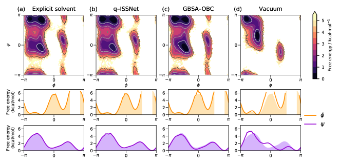
Figure 3: Two- and one-dimensional free energy plots for all-atom capped alanine systems: (a) explicit solvent system with TIP3P water model (reference), the implicit solvent setup with (b) trained q–ISSNet and (c) the GBSA–OBC model, and (d) the vacuum system without solvation treatment (used as a negative control). The 2D free energy surfaces are created by histogramming of simulation trajectories on $\phi$- and $\psi$-dihedral angles with MSM-reweighting, while the two 1-d free energy curves (bold lines) below each contour plot show the corresponding marginal distributions. For clear comparison of the 1-d distributions between the reference system and the rest, we let the shaded regions represent the explicit solvent result.

By comparing the free energy landscapes with those from the reference explicitly solvated and vacuum systems, we can assess how well the implicit solvent model can approximate the solvent effects on thermodynamics. Figure 3 shows the free energy surfaces for the implicit solvent, reference explicit solvent and vacuum systems. The free energy plots for systems with trained t-ISSNet and qt-ISSNet models can be found in Section S2 in the SI. Qualitatively, the free energy landscapes of the implicit solvent simulations (Fig. 3 b and 3 c) are dramatically different from the vacuum case (Fig. 3d), and recovers the main energy minima emerging in the explicit solvent simulation (Fig. 3a). The sample proportion in these regions in implicit solvent simulations also appears similar to the distribution for the explicit solvent system, both on the 2D free energy landscapes and on the marginal distributions for $\phi$ and $\psi$. The result proves that either of the two implicit solvent models can properly model the solvent effect, which is absent in the vacuum simulation. Between the implicit solvent systems (with our trained neural network model and with the GBSA–OBC model), it is observed that the q-ISSNet model corresponds to a free energy contour that better resembles the explicit solvent reference. The other two variant of ISSNet models, although gives slightly less accurate free energy lanscapes, but still outperform the GBSA–OBC model (see Fig. S2 in the SI).

Table 1: KL divergence, JS divergence and MSE of free energy for comparing the discrete conformational distributions on the $\phi-\psi$ plane of the implicit solvent, vacuum and the explicit solvent systems for capped alanine. Calculation is performed over the simulation trajectories after MSM reweighting (details in the SI, Section C). Bold font is designated for the lowest divergence/error values, which correspond to the implicit solvent model with ISSNet plus partial charge-only (q-) embeddings.

System	$D_{\textrm{KL}}$$/10^{-2}$		$D_{\textrm{JS}}$$/10^{-3}$		$\mathrm{MSE}$$/10^{-2}$
Explicit solvent	(0.	)	(0.	)	(0.	)
t–ISSNet	2.	32	5.	62	8.	28
q–ISSNet	1.	46	3.	63	7.	64
qt–ISSNet	5.	61	13.	4	9.	44
GBSA–OBC	9.	47	23.	4	19.	2
Vacuum	169.		530.		250.

The difference between implicit solvent models can be better analyzed by directly comparing the discretized equilibrium distributions (i.e., the histograms) on the dihedral plane, which we used to generate the free energy contours above. We evaluate the Kullback-Leibler (KL) and Jensen-Shannon (JS) divergences between the distributions of various models and that of the reference distribution, as well as the mean squared error (MSE) of discrete free energies. Table 1 presents these quantitative metrics for measuring the similarity of the free energy landscapes between the implicit solvent or the baseline vacuum system with the reference explicit solvent case. All three columns give the same trend: ISSNet implicit solvent models have the smallest, vacuum energies the largest errors, with the GBSA–OBC implicit solvent model in between. This is consistent with the visual comparison of the free energy surfaces in Fig. 3, and indicates that our machine-learned implicit solvent method outperforms the traditional GBSA–OBC model for this system. Additionally, the q-ISSNet variant (with charge-only embedding) corresponds to the smallest difference from the reference among the ISSNet models.

III.2 Chignolin

Due to their small size and short folding time, the artificially designed miniprotein chignolin (Honda et al., 2004) and its stabler variant CLN025,(Honda et al., 2008) are widely used as example systems in both experimental (Davis et al., 2012; Honda et al., 2008) and computational investigations (Satoh et al., 2006; Suenaga et al., 2007; Lindorff-Larsen et al., 2011; Nguyen et al., 2014) of protein folding and kinetics. Additionally, thanks to the availability of extensive reference data from experiments,(Honda et al., 2008) chignolin variants serve as benchmark systems in the development of all-atom force fields (Maier et al., 2015; Harder et al., 2016; Huang et al., 2017) and for comparison among force fields (Kührová et al., 2012) and solvent methods.(Anandakrishnan et al., 2015) In this section we use the CLN025 variant (Honda et al., 2008) of chignolin, a 10-amino-acid miniprotein with sequence YYDPETGTWY (together with N- and C-terminal caps) as the solute molecule, which is referred to simply as chignolin in the text below. The explicit solvent all-atom simulation trajectories (available online (Culubret and Fabritiis, 2021)) and corresponding force data were kindly provided by the authors of Ref. Wang et al., 2019b. The simulation setup is reported in the SI, Section A. We randomly selected $2\times 10^{5}$ coordinate–solvation force pairs from the aggregated data set (with $1.8\times 10^{6}$ pairs in total) according to the equilibrium conformational distribution estimated by a MSM for training and validation of ISSNet models, and divide them to four folds of equal sizes.

The training and cross-validation procedures for chignolin are similar to those for capped alanine with slightly modified setups (see Section B of the SI). In addition to the embedding choices, the number of interaction blocks also appears to be influential to the CV–FM errors in hyperparameter searches (see Table S3). Therefore, we trained the ISSNet models with the three different types of embeddings and two or three interaction blocks, resulting in six implicit solvent models for the next step.

We performed vacuum and implicit solvent simulations for chignolin (the latter with the trained ISSNet models), similar to those for capped alanine. In order to facilitate transitions among metastable states and thus a more accurate estimate of the state population with multiple short-time simulations, we applied parallel tempering (PT) methods in the MD simulations. We also performed a simulation with the GBSA–OBC model, and compared the outcome with those corresponding to the ISSNet models. All simulations were initiated from the same 16 starting structures, while were sampled from the with MSM weights. More information regarding the simulation setups can be found in the SI, Section A.

In order to visualize the conformational distribution, we performed time-lagged independent component analysis (TICA) (Pérez-Hernández et al., 2013; Schwantes and Pande, 2013) on the explicit solvent trajectories according to Ref. Husic et al., 2020 (over the pairwise C_α distances),(Husic et al., 2020) and used the resulting TICA matrix to project the simulation results for each model onto the same set of collective coordinates. The first two time-lagged independent components (TICs) resolve the three metastable states (see Fig. 4; cf. figures in Ref. Husic et al., 2020). Furthermore, a MSM is estimated on the explicit solvent simulation data to obtain the correct weights for each frame in the trajectories, such that we can more precisely estimate the free energy landscape at equilibrium by histogramming (also used for capped alanine). Free energy estimates for other systems in the comparison does not require MSM-reweighting, since a sufficient and correct sampling from the Boltzmann distribution is obtained by means of the PT simulation. Apart from the change of coordinates, the plotting procedure (see Section C of the SI) is the same as described for capped alanine.

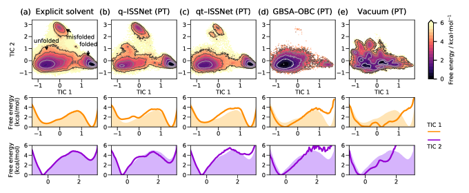
Figure 4: Two- and one-dimensional free energy plots for all-atom chignolin systems: (a) explicit solvent system with mTIP3P water model (reference), the implicit solvent setup with (b) trained q–ISSNet, (c) trained qt–ISSNet and (d) the GBSA–OBC model, and (e) the vacuum system without solvation treatment (negative control group). The 2D free energy surfaces are created by histogramming of simulation trajectories on the first and second TICs after TICA transformation. For the explicit solvent data set, a MSM is estimated upon the short simulation trajectories, and then used for reweighting in the histogram. For simulation with ISSNet models or the vacuum simulation, we use PT–MD to increase state-transition rates. The two 1-d free energy curves (bold lines) below each contour plot show the corresponding marginal distributions. For clear comparison of the 1-d distributions between the reference system and the rest, the shaded regions represent the explicit solvent result from column a.

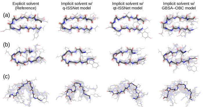
Figure 5: Representative structures of chignolin from explicit and implicit solvent simulations from (a) the folded, (b) the misfolded and (c) the unfolded metastable states. We overlay 10 structures randomly sampled from each metastable state for each solvent model (cf. Fig. 4) and visualize their backbone structures. We highlight one structure in each plot and plot its side chains in addition.

Figure 4 displays the equilibrium free energy landscapes for two ISSNet models and the reference systems we introduced above. For the convenience of description, we label the three major minima on the free energy landscape in Fig. 4a as “misfolded” (upper), “unfolded” (lower left) and “folded” (lower right) according to the folding status of the peptide conformations in these minima. These minima correspond to metastable states from MSM analyses (Husic et al., 2020) (for details see the SI, Section D). By comparing the 2D free energy plots in Fig. 4, we can qualitatively conclude that the three metastable states are present at the correct positions for all presented implicit solvent systems (Fig. 4b–d), although the misfolded state is rarely visited in the GBSA–OBC system. Meanwhile, the vacuum system has an extremely rugged free energy landscape mostly located in the unfolded region (Fig. 4e). This shows that the implicit solvent models incorporate non-trival solvent effects that are absent from the vacuum system. Another observation is that the ISSNet models better reproduce the populations of the folded and misfolded states, which are underestimated by the GBSA–OBC model. As a side note, a similar deficiency in the folded state population for chignolin has been reported and analyzed for simulation with an AMBER force field Amb, and the GBSA–OBC model.(Anandakrishnan, Izadi, and Onufriev, 2018)

In Fig. 5 we visualize some representative 3D structures of chignolin sampled from the simulation trajectories. We randomly pick 10 structures that were assigned to different metastable states on the TIC1–TIC2 plot (for details see the SI, section S4) and only plot the backbone atoms for clarity. We randomly pick one from the 10 structures for the explicit solvent reference to highlight, while for the implicit solvent structures, we highlight the one with the lowest RMSD to the explicit solvent reference. It is clear that for each metastable state, the structures are comparable between systems with explicit and implicit solvent models. Comparing structures from the folded and misfolded states (Fig. 5a and b) with the GBSA–OBC model and with ISSNet models, the local displacements across the overlayed structures from the latter are less apparent than from the former. This phenomenon corresponds to the fact that these states are correctly stabilized by the ISSNet models (cf. Fig. 4b and c).

Table 2: KL divergence, JS divergence and MSE of free energy for comparing the thermodynamics of the implicit solvent, vacuum and the explicit solvent systems for chignolin. The metrics were evaluated based on discrete conformational distributions on the TIC 1–TIC 2 plane as estimated from the simulation trajectories. In the case of explicit solvent data set, MSM-reweighting is performed. Bold font designates the lowest divergence/error values, which correspond to the implicit solvent model with ISSNet plus charge-only (q-) or type-and-charge (qt-) embeddings (cf. Figure 4b and c).

System	$D_{\textrm{KL}}$	$D_{\textrm{JS}}$	$\mathrm{MSE}$
Explicit solvent	(0.)	(0.)	(0.)
t–ISSNet	2.671/0.494	0.724/0.117	4.438/1.017
q–ISSNet${}^{\textrm{a}}$	0.221/0.366	0.053/0.086	0.432/0.526
qt–ISSNet${}^{\textrm{a}}$	0.069/0.321	0.016/0.076	0.468/0.541
GBSA–OBC	1.720	0.404	0.892
Vacuum	2.647	0.726	1.815

We quantified the comparisons between the conformational distributions of the explicit solvent systems and the different implicit solvent models with the criteria introduced for 2D free energy surfaces (see Section C in the SI). Table 2 shows that implicit solvent simulations with the ISSNet models result in lower divergences/errors with respect to the reference explicit solvent model comparing to the one with the GBSA–OBC model, indicating that ISSNet can better reproduce the thermodynamics of a solvated chignolin system.

As for the effect of hyperparameter choices, we examined the CV–FM error and the quantified differences in the free energy surfaces (Table 2). The parameters that lead to significant differences are the number of interaction blocks and the embedding strategies. Although adding a third interaction block to the models generally results with comparable or even smaller CV–FM errors (see Table S3 in the SI), except for the type-embedding ISSNet, this change does not improve the accuracy according to the three metrics. (This observation is contradictory to the claim of Ref. Wang et al., 2019b.) When other hyperparameters are held constant, using the partial charge embedding (q-) alone results in the lowest MSE of free energy, but mixed embedding (qt-) leads to the best results according to the two divergence criteria.

One of the major discrepancies in the implicit solvation methods in Fig. 4 is the relative population of the metastable states. Especially in the GBSA–OBC case, the unfolded state of chignolin is over-stabilized. We hypothesize that this behavior is mainly caused by an inaccurately predicted melting temperature $T_{m}$, which is the temperature at which the molecule is found to be folded or unfolded with equal probability in equilibrium.(Tanford, 1970; Brandts, 1964)

Table 3: Estimated folding $T_{m}$ of chignolin with different solvent models in MD simulations and experimental reference value.

Solvation model for simulation	$T_{m}$ / K
Explicit solvent (Lindorff-Larsen et al., 2011)	381(361–393)
q–ISSNet	$\sim$368/$\sim$370
qt–ISSNet${}^{\textrm{a}}$	$\sim$355/$\sim$355${}^{\textrm{b}}$
GBSA–OBC	$\sim$268/$\sim$269${}^{\textrm{b}}$
Experimental (Honda et al., 2008)	$\sim$343

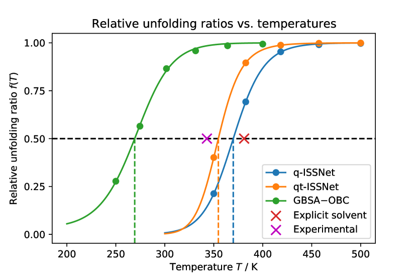
Figure 6: Relative unfolding ratio $f(T)$ for different solvent models. Here we use the constant-heat-capacity model for curve fitting. Dashed lines imply the estimated melting temperatures for each cases. Crosses visualize $T_{m}$s from explicit solvent simulation (Lindorff-Larsen et al., 2011) and experiments (Honda et al., 2008), which serve as references.

The melting temperature is defined as the temperature at which the molecule is found with equal probability in either the folded or the unfolded states. This temperature is connected to the zero-crossing of the unfolding free energy change $\Delta G(T)$, since

$$\Delta G(T)=-\beta^{-1}\log\frac{p_{\textrm{unfolded}}(T)}{p_{\textrm{folded}}(T)}.$$ (23)

Therefore, we can model the temperature dependency of $\Delta G$ from the sample distributions for the replicas at different temperatures in the PT simulations, and then solve for $T_{m}$. We utilize the two models from Ref. Schellman, 1987 for $\Delta G-T$ relationship and try to determine the parameters by curve fitting. It is straightforward to directly work on the $\Delta G-T$ plot, but the $\Delta G$ estimation from the simulations has too large uncertainty when either $p_{\textrm{unfolded}}$ or $p_{\textrm{folded}}$ is too low. Instead, we calculate and plot the relative unfolding ratio from the raw data (i.e., the solid dots in Figure 6):

$$f(T)=\frac{p_{\textrm{unfolded}}}{p_{\textrm{folded}}+p_{\textrm{unfolded}}}=\frac{1}{1+\exp\left[\beta\Delta G(T)\right]},$$ (24)

and estimate the model parameters by a least-square curve fitting. The resulted $\Delta G-T$ models give a the solid curves in Figure 6), which matches the observations from the raw data. Then we calculated the temperature corresponding to $\Delta G=0$ (i.e., when the curves cross the $f(T)=0.5$ line in Figure 6) as an estimation of $T_{m}$ (see Section E of the SI for details). The resulting $T_{m}$ for implicit solvent simulation with the ISSNet models and with the GBSA model are listed in Table 3. We also include a reference $T_{m}$ for explicit solvent simulation with the same force field and water model from Ref. Lindorff-Larsen et al., 2011 (calculated with a different approach; details in SI, Section E). This analysis shows that the traditional GBSA model dramatically underestimates the $T_{m}$, while our neural network ISSNet models result in rather accurate melting temperatures that are bracketed by the explicit solvent and experimental observations (labeled in Figure 6 as crosses). Note that our models were fitted at one single temperature and can thus not generally expected to make quantitative predictions at other temperatures. However, the good match observed in this case is a piece of evidence that the ISSNet method can learn the qualitatively correct physics.

IV Discussion

Here we provide some physical interpretation for some choices in our implementation and experiments and discuss remaining challenges that call for further investigations.

We leverage an enhanced sampling method for the estimate of the free energy landscape for chignolin simulation with trained ISSNet models. Although chignolin is usually regarded as a “fast-folder”,(Davis et al., 2012; Honda et al., 2008) transitions among the metastable states, e.g., between the folded and unfolded states, are rather slow comparing to our simulation timescale. As a reference, the all-atom explicit solvent folding and unfolding timescales for chignolin in the NVT–ensemble at 343K is reported to be 0.6 and 2.4 $\mu$s, respectively,(Lindorff-Larsen et al., 2011) which are several times longer than our simulation time. In fact, the generation of our explicit solvent reference data set was also obtained by means of an enhanced sampling method,(Wang et al., 2019b) and we reweighted the data set according to a MSM analysis in order to gain the ground truth of the Boltzmann distribution. For assessing implicit solvent models, we use the PT–MD to enable a rather accurate equilibrium sampling within short simulation time, as it speeds up the state transitions without modifying the thermodynamics at equilibrium.(Trebst, Troyer, and Hansmann, 2006; Earl and Deem, 2005)

The ISSNet approach employs a (CG)SchNet architecture with slight modification for expressing the solvation free energy. In both examples we found that embeddings (q- and qt-) involving partial atomic charge led to higher accuracy in the recovered thermodynamics than a traditional embedding (t-) based solely on the identification of the atom type (see Table 1 and 2). This result underscores the importance of including electrostatic information in the network for accurate solvent modeling. It is known that electrostatic interactions are vital for modeling solvent effects for both explicit and implicit models.(Adcock and McCammon, 2006; Onufriev and Izadi, 2018; Ren et al., 2012; Chen, Brooks, and Khandogin, 2008; Kleinjung and Fraternali, 2014) Although partial atomic charges can be learned and predicted by SchNet (Schütt et al., 2018) or other networks (Nebgen et al., 2018; Sifain et al., 2018) from merely the element-type embedding, such predictions tend to require a deep network with more interaction blocks and a variety of input molecules. Our results suggest that it is neither accurate nor efficient for an implicit solvent model to learn the electrostatics from scratch. We hypothesize that the new atomic embedding strategy may strengthen the performance and/or reduce the computational cost for some other SchNet-based molecular machine learning approaches, such as CGSchNet.

Although our ISSNet models appear more accurate than the reference methods, they are not free of limitations. Regarding the chignolin results, we observe that the metastable states are not exactly weighted, and the free energy surface for the misfolded and unfolded metastable states slightly differ from the reference. In order to tackle these problems, we experimented with different training setups, such as training set composition (e.g., distribution of training data on the space spanned by the first two TICs) and hyperparameters for SchNet architectures. We observed different simulation outcomes with resulting models (e.g., Fig. 4 b, c and Table 2), but we do not yet have an ultimate solution to consistently and systematically improve the accuracy of the free energy landscape.

We note that the CV–FM error is used to assess the models and to optimize the hyperparameters in both Refs. Wang et al., 2019b and Husic et al., 2020. In this work, however, we found that—at least for the ISSNet models for chignolin—there is no strict correspondence between the lowest CV–FM error and the highest accuracy (e.g., comparing models with different numbers of interaction blocks and embedding methods for chignolin, see Section S2 in the SI). We hypothesize that FM error on a limited data set may fail to assess the global accuracy of free energy surfaces for complex systems. High-energy regions—including transition paths—constitute only a tiny proportion of the training and validation data, because their Boltzmann probability is exponentially lower than those of major energy minima. Therefore, an erroneous prediction of the mean force in these regions does not strongly affect the overall FM loss. Nevertheless, it can cause differences in the height of energy barriers to the metastable states, resulting in an inaccurate relative free energy difference and thus a wrong weighting of free energy minima. This hypothesis also has implications on the model training and hyperparameter optimizations, because both of them rely on only the FM error but not the energy or distribution weights. In this sense, combining the variational FM method with alternative CG schemes (e.g., relative entropy (Shell, 2008; Chaimovich and Shell, 2011)) may systematically improve the accuracy of related machine learning methods.

Another aspect to be improved for the ISSNet models is the speed of simulation (see the SI, Section F). Because the forces from the neural network are required for every time step, simulations become computationally demanding and time-consuming, restricting the application of the current ISSNet model to longer simulations and larger molecules. In this work we partially avoided this problem by evaluating the ISSNet forces in batch, which speeds up the sampling but not single simulations. While this work presents an important feasibility study, future developments will involve reducing the frequency of neural network evaluation (e.g., by multiple time-step MD simulation), lowering communication overhead between the MD software and the deep-learning framework as well as finding computationally cheaper energy neural networks in substitution for SchNet.(Schütt et al., 2018)

To illustrate the advantage of the ISSNet approach, we compared it to GBSA–OBC,(Onufriev, Bashford, and Case, 2004) an existing widely-used implicit solvent model. This choice is due to the availability in simulation tools such as AMBER Amb, and OpenMM.(Eastman et al., 2017) Additionally, a recent study assures the qualitative similarity between GBSA–OBC and a newer GBNeck2 model Nguyen, Roe, and Simmerling, 2013 for the implicit solvation of chignolin (CLN025).Anandakrishnan, Izadi, and Onufriev, 2018 However, given the wealth of existing implicit solvent methods, we can not conclude that the ISSNet models trained herein reflect the state of the art for the accuracy of thermodynamics. Nevertheless, due to the variational nature of the formulation, given sufficient training data and a sufficiently competent neural network, our model shall be able to reproduce the thermodynamics of a given explicit solvent model with arbitrarily high accuracy.

Despite its success, an ISSNet model is at the moment only parameterized for a given molecular system at a fixed thermodynamic state. Even when a model successfully learns the free energy surface specific to the given system, it is not guaranteed to output sensible solvation forces for systems at a different temperature/pressure and/or consisting of other solute molecules. Although we achieved an accurate estimation of the unfolding temperature $T_{m}$ by the ISSNet models, it may merely be due to the fact that the simulation temperature for the data set generation is close to $T_{m}$. In fact, we observed that the empirical thermodynamic parameters (e.g., the enthalpy and entropy changes) from curve fitting for chignolin unfolding in implicit solvents are different from the experimental and explicit solvent results, thus leading to a significant deviation of the folded population at other temperatures (see the SI, Section E). Therefore, a proper modeling of the temperature/pressure dependence of the free energy surface is yet to be developed.

Another potential of the future development of the ISSNet method is to achieve the transferability among a larger variety of solute molecules. Since the (CG)SchNet architecture allows the same set of parameters to be shared among models for different systems,(Husic et al., 2020; Schütt et al., 2018) it is in principle feasible to optimize ISSNet models for a more general description of the solvent effects. Note that a variety of systems may also provide information for correctly treating the conformations that are under-sampled in case of a single training system, thus beneficial to the accuracy in free-energy modeling at the same time. By training on extended data sets (e.g., a set of peptides or proteins) and potentially incorporating more insights from statistical physics, we may train more transferable yet accurate solvation models and widen the application of the ISSNet approach.

V Conclusions

In this work, we have reformulated the implicit solvation modeling as a bottom-up coarse graining problem, and shown that an accurate implicit solvent model can be machine-learned by leveraging the variational FM approach. Based on the CGnet (Wang et al., 2019b) and CGSchNet (Husic et al., 2020) methods established for machine learning of CG potentials, we develop ISSNet for learning an implicit solvent model from explicit solvent simulation data. Our method outperforms the GBSA–OBC model (Onufriev, Bashford, and Case, 2004)—an widely used implicit solvent method—on two biomolecular benchmark systems (capped alanine and chignolin) in terms of accuracy. Our novel method sets up a stage for utilizing the power of machine learning to the implicit solvent problem, and we expect further development on the transferability among thermodynamic states and chemical space to widen its application.

Supporting Information

Detailed setups for model training and simulation, as well as procedures for various analyses that are referred to in the main text can be found in the online supplementary material.

Data Availability

The data that support the findings of this study are available from the corresponding author upon reasonable request.

References

- Laage, Elsaesser, and Hynes (2017) D. Laage, T. Elsaesser, and J. T. Hynes, Chem. Rev. 117, 10694 (2017).
- Lewandowski et al. (2015) J. R. Lewandowski, M. E. Halse, M. Blackledge, and L. Emsley, Science 348, 578 (2015).
- Daniel, Finney, and Stoneham (2004) R. M. Daniel, J. L. Finney, and M. Stoneham, Philosophical Transactions of the Royal Society of London. Series B: Biological Sciences (2004).
- Ball (2008) P. Ball, Chem. Rev. 108, 74 (2008).
- Kalinowska et al. (2017) B. Kalinowska, M. Banach, Z. Wiśniowski, L. Konieczny, and I. Roterman, J. Mol. Model. 23 (2017), 10.1007/s00894-017-3367-z.
- Barron, Hecht, and Wilson (1997) L. D. Barron, L. Hecht, and G. Wilson, Biochemistry 36, 13143 (1997).
- Levy and Onuchic (2006) Y. Levy and J. N. Onuchic, Annu. Rev. Biophys. Biomol. Struct. 35, 389 (2006).
- Ben-Naim (2002) A. Ben-Naim, Biophys. Chem. 101, 309 (2002).
- Persch, Dumele, and Diederich (2015) E. Persch, O. Dumele, and F. Diederich, Angew. Chem. Int. Ed. 54, 3290 (2015).
- Ladbury (1996) J. E. Ladbury, Chem. Biol. 3, 973 (1996).
- Adcock and McCammon (2006) S. A. Adcock and J. A. McCammon, Chem. Rev. 106, 1589 (2006).
- Dror et al. (2012) R. O. Dror, R. M. Dirks, J. P. Grossman, H. Xu, and D. E. Shaw, Annu. Rev. Biophys. 41, 429 (2012).
- Braun et al. (2018) E. Braun, J. Gilmer, H. B. Mayes, D. L. Mobley, J. I. Monroe, S. Prasad, and D. M. Zuckerman, LiveCoMS 1, 5957 (2018).
- Brooijmans and Kuntz (2003) N. Brooijmans and I. D. Kuntz, Annu. Rev. Biophys. Biomol. Struct. 32, 335 (2003).
- Onufriev and Izadi (2018) A. V. Onufriev and S. Izadi, Wiley Interdiscip. Rev. Comput. Mol. Sci. 8, e1347 (2018).
- Ren et al. (2012) P. Ren, J. Chun, D. G. Thomas, M. J. Schnieders, M. Marucho, J. Zhang, and N. A. Baker, Q. Rev. Biophys. 45, 427 (2012).
- Anandakrishnan et al. (2015) R. Anandakrishnan, A. Drozdetski, R. C. Walker, and A. V. Onufriev, Biophys. J. 108, 1153 (2015).
- Baptista, Teixeira, and Soares (2002) A. M. Baptista, V. H. Teixeira, and C. M. Soares, J. Chem. Phys. 117, 4184 (2002).
- Mongan, Case, and McCammon (2004) J. Mongan, D. A. Case, and J. A. McCammon, J. Comput. Chem. 25, 2038 (2004).
- Trebst, Troyer, and Hansmann (2006) S. Trebst, M. Troyer, and U. H. Hansmann, J. Chem. Phys. 124, 174903 (2006).
- Earl and Deem (2005) D. J. Earl and M. W. Deem, Phys. Chem. Chem. Phys. 7, 3910 (2005).
- Śledź and Caflisch (2018) P. Śledź and A. Caflisch, Curr. Opin. Struct. Biol. 48, 93 (2018).
- Wang et al. (2019a) E. Wang, H. Sun, J. Wang, Z. Wang, H. Liu, J. Z. Zhang, and T. Hou, Chem. Rev. 119, 9478 (2019a).
- Hawkins, Cramer, and Truhlar (1996) G. D. Hawkins, C. J. Cramer, and D. G. Truhlar, J. Chem. Phys. 100, 19824 (1996).
- Roe et al. (2007) D. R. Roe, A. Okur, L. Wickstrom, V. Hornak, and C. Simmerling, J. Phys. Chem. B 111, 1846 (2007).
- (26) 2020 Amber Reference Manual.
- Lee, Salsbury Jr, and Brooks III (2002) M. S. Lee, F. R. Salsbury Jr, and C. L. Brooks III, J Chem. Phys. 116, 10606 (2002).
- Lee et al. (2003) M. S. Lee, M. Feig, F. R. Salsbury Jr, and C. L. Brooks III, J. Comput. Chem. 24, 1348 (2003).
- Im, Lee, and Brooks III (2003) W. Im, M. S. Lee, and C. L. Brooks III, J. Comput. Chem. 24, 1691 (2003).
- Brooks et al. (2009) B. R. Brooks, C. L. Brooks III, A. D. Mackerell Jr, L. Nilsson, R. J. Petrella, B. Roux, Y. Won, G. Archontis, C. Bartels, S. Boresch, et al., J. Comput. Chem. 30, 1545 (2009).
- Knight and Brooks III (2011) J. L. Knight and C. L. Brooks III, J. Comput. Chem. 32, 2909 (2011).
- Cumberworth, Bui, and Gsponer (2016) A. Cumberworth, J. M. Bui, and J. Gsponer, J. Comput. Chem. 37, 629 (2016).
- Zhou and Berne (2002) R. Zhou and B. J. Berne, Proc. Natl. Acad. Sci. U. S. A. 99, 12777 (2002).
- Nymeyer and Garcia (2003) H. Nymeyer and A. E. Garcia, Proc. Natl. Acad. Sci. U. S. A. 100, 13934 (2003).
- Zhou (2003) R. Zhou, Proteins 53, 148 (2003).
- Clementi, Nymeyer, and Onuchic (2000) C. Clementi, H. Nymeyer, and J. N. Onuchic, J. Mol. Biol. 298, 937 (2000).
- Clementi (2008) C. Clementi, Curr. Opin. Struct. Biol. 18, 10 (2008).
- Saunders and Voth (2013) M. G. Saunders and G. A. Voth, Annu. Rev. Bioph. Biom. 42, 73 (2013).
- Noid (2013) W. G. Noid, J. Chem. Phys. 139, 090901 (2013).
- Ingólfsson et al. (2014) H. I. Ingólfsson, C. A. Lopez, J. J. Uusitalo, D. H. de Jong, S. M. Gopal, X. Periole, and S. J. Marrink, WIREs Comput. Mol. Sci. 4, 225 (2014).
- Kmiecik et al. (2016) S. Kmiecik, D. Gront, M. Kolinski, L. Wieteska, A. E. Dawid, and A. Kolinski, Chem. Rev. 116, 7898 (2016).
- Pak and Voth (2018) A. J. Pak and G. A. Voth, Curr. Opin. Struc. Biol. 52, 119 (2018).
- Chen et al. (2018) J. Chen, J. Chen, G. Pinamonti, and C. Clementi, J. Chem. Theory Comput. 14, 3849 (2018).
- Singh and Li (2019) N. Singh and W. Li, Int. J. Mol. Sci. 20 (2019), 10.3390/ijms20153774.
- Nüske, Boninsegna, and Clementi (2019) F. Nüske, L. Boninsegna, and C. Clementi, J. Chem. Phys. 151, 044116 (2019).
- Wang et al. (2019b) J. Wang, S. Olsson, C. Wehmeyer, A. Pérez, N. E. Charron, G. de Fabritiis, F. Noé, and C. Clementi, ACS Cent. Sci. 5, 755 (2019b).
- Wang et al. (2020) J. Wang, S. Chmiela, K.-R. Müller, F. Noé, and C. Clementi, J. Chem. Phys. 152, 194106 (2020).
- Husic et al. (2020) B. E. Husic, N. E. Charron, D. Lemm, J. Wang, A. Pérez, M. Majewski, A. Krämer, Y. Chen, S. Olsson, G. de Fabritiis, F. Noé, and C. Clementi, J. Chem. Phys. 153, 194101 (2020).
- Farrell, Oden, and Faghihi (2015) K. Farrell, J. T. Oden, and D. Faghihi, J. Comput. Phys. 295, 189 (2015).
- Boninsegna, Banisch, and Clementi (2018) L. Boninsegna, R. Banisch, and C. Clementi, J. Chem. Theory Comput. 14, 453 (2018).
- Izvekov and Voth (2005) S. Izvekov and G. A. Voth, J. Phys. Chem. B 109, 2469 (2005).
- Noid et al. (2008a) W. G. Noid, J.-W. Chu, G. S. Ayton, V. Krishna, S. Izvekov, G. A. Voth, A. Das, and H. C. Andersen, J. Chem. Phys. 128, 244114 (2008a).
- LeCun, Bengio, and Hinton (2015) Y. LeCun, Y. Bengio, and G. Hinton, Cah. Rev. The. 521, 436 (2015).
- Butler et al. (2018) K. T. Butler, D. W. Davies, H. Cartwright, O. Isayev, and A. Walsh, Nature 559, 547 (2018).
- Noé et al. (2020) F. Noé, A. Tkatchenko, K.-R. Müller, and C. Clementi, Annu. Rev. Phys. Chem. 71, 361 (2020).
- Behler (2016) J. Behler, J. Chem. Phys. 145, 170901 (2016).
- Chmiela et al. (2018) S. Chmiela, H. E. Sauceda, K.-R. Müller, and A. Tkatchenko, Nat. Commun. 9, 1 (2018).
- Wang and Gómez-Bombarelli (2019) W. Wang and R. Gómez-Bombarelli, npj Comput. Mater. 5, 1 (2019).
- Zhang et al. (2018) L. Zhang, J. Han, H. Wang, R. Car, and W. E, J. Chem. Phys. 149, 034101 (2018).
- Wang et al. (2021) J. Wang, N. Charron, B. Husic, S. Olsson, F. Noé, and C. Clementi, J. Chem. Phys. 154, 164113 (2021).
- Schütt et al. (2018) K. T. Schütt, H. E. Sauceda, P.-J. Kindermans, A. Tkatchenko, and K.-R. Müller, J. Chem. Phys. 148, 241722 (2018).
- Basdogan et al. (2019) Y. Basdogan, M. C. Groenenboom, E. Henderson, S. De, S. B. Rempe, and J. A. Keith, J. Chem. Theory Comput. 16, 633 (2019).
- Chan et al. (2019) H. Chan, M. J. Cherukara, B. Narayanan, T. D. Loeffler, C. Benmore, S. K. Gray, and S. K. Sankaranarayanan, Nat. Commun. 10, 1 (2019).
- Patra et al. (2019) T. K. Patra, T. D. Loeffler, H. Chan, M. J. Cherukara, B. Narayanan, and S. K. Sankaranarayanan, Appl. Phys. Lett. 115, 193101 (2019).
- Mahmoud et al. (2020) S. S. M. Mahmoud, G. Esposito, G. Serra, and F. Fogolari, Bioinformatics 36, 1757 (2020).
- Bottaro, Lindorff-Larsen, and Best (2013) S. Bottaro, K. Lindorff-Larsen, and R. B. Best, J. Chem. Theory Comput. 9, 5641 (2013).
- Honda et al. (2008) S. Honda, T. Akiba, Y. S. Kato, Y. Sawada, M. Sekijima, M. Ishimura, A. Ooishi, H. Watanabe, T. Odahara, and K. Harata, J. Am. Chem. Soc. 130, 15327 (2008).
- Onufriev, Bashford, and Case (2004) A. Onufriev, D. Bashford, and D. A. Case, Proteins 55, 383 (2004).
- Kirkwood (1935) J. G. Kirkwood, J. Chem. Phys. 3, 300 (1935).
- Roux and Simonson (1999) B. Roux and T. Simonson, Biophys. Chem. 78, 1 (1999).
- Chen, Brooks, and Khandogin (2008) J. Chen, C. L. Brooks, and J. Khandogin, Curr. Opin. Struct. Biol. 18, 140 (2008).
- Feig, Tanizaki, and Sayadi (2008) M. Feig, S. Tanizaki, and M. Sayadi, Annual Reports in Computational Chemistry 4, 107 (2008).
- Kleinjung and Fraternali (2014) J. Kleinjung and F. Fraternali, Curr. Opin. Struct. Biol. 25, 126 (2014).
- Born (1920) M. Born, Z. Phys. 1, 45 (1920).
- Onufriev and Case (2019) A. V. Onufriev and D. A. Case, Annu. Rev. Biophys. 48, 275 (2019).
- Tsui and Case (2000) V. Tsui and D. A. Case, Biopolymers 56, 275 (2000).
- Qiu et al. (1997) D. Qiu, P. S. Shenkin, F. P. Hollinger, and W. C. Still, J. Phys. Chem. A 101, 3005 (1997).
- Levy et al. (2003) R. M. Levy, L. Y. Zhang, E. Gallicchio, and A. K. Felts, J. Am. Chem. Soc. 125, 9523 (2003).
- Izvekov and Voth (2009) S. Izvekov and G. A. Voth, J. Phys. Chem. B 113, 4443 (2009).
- Cao et al. (2013) Z. Cao, J. F. Dama, L. Lu, and G. A. Voth, J. Chem. Theory Comput. 9, 172 (2013).
- Noid et al. (2008b) W. G. Noid, P. Liu, Y. Wang, J.-W. Chu, G. S. Ayton, S. Izvekov, H. C. Andersen, and G. A. Voth, J. Chem. Phys. 128, 244115 (2008b).
- Note (1) In the regularized variant, there is also a prior energy to avoid physically unfavorable states.(Wang et al., 2019b).
- Hastie, Tibshirani, and Friedman (2009) T. Hastie, R. Tibshirani, and J. Friedman, The Elements of Statistical Learning (Springer, New York, NY, 2009).
- Kingma and Ba (2014) D. P. Kingma and J. Ba, ArXiv e-prints (2014), 1412.6980 .
- Eastman et al. (2017) P. Eastman, J. Swails, J. D. Chodera, R. T. McGibbon, Y. Zhao, K. A. Beauchamp, L.-P. Wang, A. C. Simmonett, M. P. Harrigan, C. D. Stern, et al., PLoS Comput. Biol. 13, e1005659 (2017).
- Eastman (2020) P. Eastman, “openmm-torch,” (2020), [Online; accessed 7. Jan. 2021].
- Swendsen and Wang (1986) R. H. Swendsen and J.-S. Wang, Phys. Rev. Lett. 57, 2607 (1986).
- Sugita and Okamoto (1999) Y. Sugita and Y. Okamoto, Chem. Phys. Lett. 314, 141 (1999).
- Zuckerman (2011) D. M. Zuckerman, Annu. Rev. Biophys. 40, 41 (2011).
- Bernardi, Melo, and Schulten (2015) R. C. Bernardi, M. C. R. Melo, and K. Schulten, Biochim. Biophys. Acta Gen. Subj. 1850, 872 (2015).
- Note (2) Code that facilitated the experiments in the paper: https://github.com/noegroup/reform/releases/tag/v0.1.
- Apostolakis, Ferrara, and Caflisch (1999) J. Apostolakis, P. Ferrara, and A. Caflisch, J. Chem. Phys. 110, 2099 (1999).
- Feig (2008) M. Feig, J. Chem. Theory Comput. 4, 1555 (2008).
- Pettitt and Karplus (1985) B. M. Pettitt and M. Karplus, Chem. Phys. Lett. 121, 194 (1985).
- Tobias and Brooks III (1992) D. J. Tobias and C. L. Brooks III, J. Phys. Chem. 96, 3864 (1992).
- Anderson and Hermans (1988) A. G. Anderson and J. Hermans, Proteins 3, 262 (1988).
- Drozdov, Grossfield, and Pappu (2004) A. N. Drozdov, A. Grossfield, and R. V. Pappu, J. Am. Chem. Soc. 126, 2574 (2004).
- Prinz et al. (2011) J.-H. Prinz, H. Wu, M. Sarich, B. Keller, M. Senne, M. Held, J. D. Chodera, C. Schütte, and F. Noé, J. Chem. Phys. 134, 174105 (2011).
- Wehmeyer et al. (2018) C. Wehmeyer, M. K. Scherer, T. Hempel, B. E. Husic, S. Olsson, and F. Noé, LiveCoMS 1, 5965 (2018).
- Scherer et al. (2015) M. K. Scherer, B. Trendelkamp-Schroer, F. Paul, G. Pérez-Hernández, M. Hoffmann, N. Plattner, C. Wehmeyer, J.-H. Prinz, and F. Noé, J. Chem. Theory Comput. 11, 5525 (2015).
- Honda et al. (2004) S. Honda, K. Yamasaki, Y. Sawada, and H. Morii, Structure 12, 1507 (2004).
- Davis et al. (2012) C. M. Davis, S. Xiao, D. P. Raleigh, and R. B. Dyer, J. Am. Chem. Soc. 134, 14476 (2012).
- Satoh et al. (2006) D. Satoh, K. Shimizu, S. Nakamura, and T. Terada, FEBS Lett. 580, 3422 (2006).
- Suenaga et al. (2007) A. Suenaga, T. Narumi, N. Futatsugi, R. Yanai, Y. Ohno, N. Okimoto, and M. Taiji, Chem. Asian J. 2, 591 (2007).
- Lindorff-Larsen et al. (2011) K. Lindorff-Larsen, S. Piana, R. O. Dror, and D. E. Shaw, Science 334, 517 (2011).
- Nguyen et al. (2014) H. Nguyen, J. Maier, H. Huang, V. Perrone, and C. Simmerling, J. Am. Chem. Soc. 136, 13959 (2014).
- Maier et al. (2015) J. A. Maier, C. Martinez, K. Kasavajhala, L. Wickstrom, K. E. Hauser, and C. Simmerling, J. Chem. Theory Comput. 11, 3696 (2015).
- Harder et al. (2016) E. Harder, W. Damm, J. Maple, C. Wu, M. Reboul, J. Y. Xiang, L. Wang, D. Lupyan, M. K. Dahlgren, J. L. Knight, et al., J. Chem. Theory Comput. 12, 281 (2016).
- Huang et al. (2017) J. Huang, S. Rauscher, G. Nawrocki, T. Ran, M. Feig, B. L. de Groot, H. Grubmüller, and A. D. MacKerell, Nat. Methods 14, 71 (2017).
- Kührová et al. (2012) P. Kührová, A. De Simone, M. Otyepka, and R. B. Best, Biophys. J. 102, 1897 (2012).
- Culubret and Fabritiis (2021) A. P. Culubret and G. D. Fabritiis, (2021), 10.6084/m9.figshare.13858898.v1.
- Pérez-Hernández et al. (2013) G. Pérez-Hernández, F. Paul, T. Giorgino, G. De Fabritiis, and F. Noé, J. Chem. Phys. 139, 07B604_1 (2013).
- Schwantes and Pande (2013) C. R. Schwantes and V. S. Pande, J. Chem. Theory Comput. 9, 2000 (2013).
- Anandakrishnan, Izadi, and Onufriev (2018) R. Anandakrishnan, S. Izadi, and A. V. Onufriev, J. Chem. Theory Comput. 15, 625 (2018).
- Tanford (1970) C. Tanford, Adv. Protein Chem. 24, 1 (1970).
- Brandts (1964) J. F. Brandts, J. Am. Chem. Soc. 86, 4291 (1964).
- Schellman (1987) J. A. Schellman, Ann. Rev. Biophys. Biophys. Chem. 16, 115 (1987).
- Nebgen et al. (2018) B. Nebgen, N. Lubbers, J. S. Smith, A. E. Sifain, A. Lokhov, O. Isayev, A. E. Roitberg, K. Barros, and S. Tretiak, J. Chem. Theory Comput. 14, 4687 (2018).
- Sifain et al. (2018) A. E. Sifain, N. Lubbers, B. T. Nebgen, J. S. Smith, A. Y. Lokhov, O. Isayev, A. E. Roitberg, K. Barros, and S. Tretiak, J. Phys. Chem. Lett. 9, 4495 (2018).
- Shell (2008) M. S. Shell, J. Chem. Phys. 129, 144108 (2008).
- Chaimovich and Shell (2011) A. Chaimovich and M. S. Shell, J. Chem. Phys. 134, 094112 (2011).
- Nguyen, Roe, and Simmerling (2013) H. Nguyen, D. R. Roe, and C. Simmerling, J. Chem. Theory Comput. 9, 2020 (2013).
- Schrödinger, LLC (2015) Schrödinger, LLC, “The PyMOL molecular graphics system, version 1.8,” (2015).