The Effect of Inefficient Accretion on Planetary Differentiation

Abstract

Pairwise collisions between terrestrial embryos are the dominant means of accretion during the last stage of planet formation. Hence, their realistic treatment in N-body studies is critical to accurately model the formation of terrestrial planets and to develop interpretations of telescopic and spacecraft observations. In this work, we compare the effects of two collision prescriptions on the core-mantle differentiation of terrestrial planets: a model in which collisions are always completely accretionary (“perfect merging”) and a more realistic model based on neural networks that has been trained on hydrodynamical simulations of giant impacts. The latter model is able to predict the loss of mass due to imperfect accretion and the evolution of non-accreted projectiles in hit-and-run collisions. We find that the results of the neural-network model feature a wider range of final core mass fractions and metal-silicate equilibration pressures, temperatures, and oxygen fugacities than the assumption of perfect merging. When used to model collisions in N-body studies of terrestrial planet formation, the two models provide similar answers for planets more massive than $0.1\text{\,}\mathrm{M_{\oplus}}$ (Earth’s masses). For less massive final bodies, however, the inefficient-accretion model predicts a higher degree of compositional diversity. This phenomenon is not reflected in planet formation models of the solar system that use perfect merging to determine collisional outcomes. Our findings confirm the role of giant impacts as important drivers of planetary diversity and encourage a realistic implementation of inefficient accretion in future accretion studies.

tablenum SIXtablenum

1 Introduction

Collisions between similar-size planetary bodies (“giant impacts”) dominate the final stage of planet formation (Wetherill, 1985; Asphaug, 2010). These events generally result in the formation of transient magma oceans on the resulting bodies (Tonks & Melosh, 1993; de Vries et al., 2016). During the last decade, a series of studies combined core-mantle differentiation with accretion modeling to put constraints on how terrestrial planets’ cores formed in the solar system and showed that core formation of terrestrial planets does not occur in a single stage, but rather that it is the result of a multistage process, i.e., a series of metal-silicate equilibrations (e.g., Rubie et al., 2011, 2015; Dwyer et al., 2015; Bonsor et al., 2015; Carter et al., 2015; Rubie et al., 2016; Fischer et al., 2017; Zube et al., 2019). In particular, the core formation model from Rubie et al. (2015) uses rigorous chemical mass balance with metal-silicate element partitioning data and requires assumptions regarding the bulk compositions of all starting embryos and planetesimals as a function of heliocentric distance. The differentiation of terrestrial planets is modeled as the separation of the iron-rich metal from silicate material using metal-silicate partitioning of elements to determine the evolving chemistry of the two reservoirs. New insights into terrestrial planet formation have been enabled by this equilibration model. For example, Rubie et al. (2015) demonstrated that Earth likely accreted from heterogeneous reservoirs of early solar system materials, Rubie et al. (2016) demonstrated that iron sulfide segregation was responsible for stripping the highly siderophile elements from Earth’s mantle, and Jacobson et al. (2017) proposed that Venus does not have an active planetary dynamo because it never experienced late Moon-forming giant impacts.

These previous studies of planet differentiation interpreted the results of N-body simulations of terrestrial planet formation where collisions were treated as perfectly inelastic, which computer models of giant impacts have shown is an oversimplification of the complex collision process (e.g., Agnor & Asphaug, 2004; Stewart & Leinhardt, 2012). Inelastic collisions, or “perfect merging”, assumes the projectile mass ($M_{\mathrm{P}}$) merges with the target mass ($M_{\mathrm{T}}$) to form a body with mass $M_{\mathrm{T}}+M_{\mathrm{P}}$. However, in nearly all giant impacts, escaping debris is produced, and the projectile’s core does not simply descend through the magma ocean and merge with the target’s metal core. Instead, half of all collisions are ‘hit-and-run’, where the projectile escapes accretion (Agnor & Asphaug, 2004; Kokubo & Genda, 2010) and may never re-impact the target again (Chambers, 2013; Emsenhuber et al., 2020). In these events, partial accretion may occur between the metal and silicate reservoirs of the target body and the projectile (or ‘runner’). To accurately model the geochemical evolution of the mantles and cores of growing planetary bodies, it is thus necessary to account for the range of accretionary (or non-accretionary) outcomes of giant impacts.

1.1 Beyond perfect merging

High-resolution hydrocode computer simulations of collisions provide a description of the outcomes of giant impacts, which can then be incorporated into planet formation models to produce higher-fidelity predictions. But each giant impact simulation requires a long computational time to complete (on the order of hours to days depending on the resolution and computing resources). Since a large number of collisions may occur during late-stage terrestrial planet formation (up to order of ${10}^{3}$, e.g., Emsenhuber et al., 2020), it is impractical to model each impact “on-the-fly” by running a full hydrocode simulation at a resolution that is sufficient to make meaningful predictions.

Several previous studies focused on overcoming both the assumption of perfect merging and the aforementioned computational bottleneck. These works employed various techniques to resolve different aspects of giant impacts. Commonly, scaling laws and other algebraic relationships (e.g. Holsapple & Housen, 1986; Housen & Holsapple, 1990; Holsapple, 1994; Kokubo & Genda, 2010; Leinhardt & Stewart, 2012; Genda et al., 2017) are utilized during an N-body (orbital dynamical) planet formation simulation to predict the collision outcome for the masses of post-impact remnants (e.g. Chambers, 2013; Quintana et al., 2016; Clement et al., 2019). The post-impact information is then fed back into the N-body code for further dynamical evolution. Other studies ‘handed off’ each collision scenario to a hydrodynamic simulation in order to model the exact impact scenario explicitly, and fed post-impact information back to the N-body code (Genda et al., 2017; Burger et al., 2020). The latter methodology is the most rigourous, but also the most computationally demanding, as it requires to run a hydrodynamic calculation for every one of the hundreds of collisions in an N-body simulation, each of which requires days of computer time when using modest resolution.

Alternatively, Cambioni et al. (2019, termed C19 hereafter) proposed a fully data-driven approach, in which machine-learning algorithms were trained on a data set of pre-existing hydrocode simulations (Reufer, 2011; Gabriel et al., 2020). The machine-learned functions (“surrogate models”) predict the outcome of a collision within a known level of accuracy with respect to the hydrocode simulations in an independent testing set. This process is fully data-driven and does not introduce model assumptions in the fitting, which is in contrast to scaling laws composed of a set of algebraic functions based on physical arguments (e.g., Leinhardt & Stewart, 2012; Gabriel et al., 2020). The surrogate models are fast predictors and Emsenhuber et al. (2020, termed E20 hereafter) implemented them in a code library named collresolve (Emsenhuber & Cambioni, 2019) to realistically treat collisions on-the-fly during terrestrial planet formation studies. When collresolve is used to treat collisions in N-body studies, the final planets feature a wider range of masses and degree of mixing across feeding zones in the disk compared with those predicted by assuming perfect merging. Although E20 ignored debris re-accretion —and we use these dynamical simulations for the study herein— their results suggest that composition diversity increases in collision remnants. This is something that cannot be predicted by models that assume perfect merging.

1.2 This work

In this paper, we compare the collision outcome obtained assuming perfect merging with that predicted by the more realistic machine-learned giant impact model of C19 and E20. In the former case, debris is not produced by definition and in the latter case, debris is produced but not re-accreted. In this respect, our goal is not to reproduce the solar system terrestrial planets, but to investigate whether or not the two collision models produce different predictions in terms of terrestrial planets’ core-mantle differentiation at the end of the planetary system’s dynamical evolution.

C19 and E20 developed models for the mass and orbits of the largest post-impact remnants; here we go a step further and develop a model for the preferential erosion of mantle silicates and core materials. To do so, we train two new neural networks to predict the core mass fraction of the resulting bodies of a giant impact. We describe the data-driven model of inefficient accretion by C19 and E20 in Section 2 and its implementation in the core-mantle differentiation model by Rubie et al. (2015) in Section 3.

We compare the perfect merging and inefficient-accretion models in two ways: (1) by studying the case of a single collision between two planetary embryos (Section 4); and (2) by interpreting the effect of multiple giant impacts in the N-body simulations of accretion presented in E20 (Section 5). During the accretion of planets through giant impacts between planetary embryos, we focus on the evolution of those variables that control planetary differentiation: mass, core mass fraction, as well as metal-silicate equilibration pressure, temperature, and oxygen fugacity. Other factors that may alter composition and thermodynamical evolution indirectly, e.g., atmospheric escape and radiative effects, are not covered in these models.

2 Inefficient-accretion model

The data-driven inefficient-accretion model by C19 and E20 consists of applying machine learning to the prediction of giant impacts’ outcomes based on the pre-existing set of collision simulations described below in Section 2.1. By training on a large data set of simulations of giant impacts, this approach allows producing response functions (surrogate models) that accurately and quickly predict key outcomes of giant impacts needed to introduce realistic collision outcomes “on-the-fly” of an N-body code.

2.1 Data set of giant impact simulations

The data set used in C19 and E20 and in this work is composed of nearly 800 simulations of planetary collisions performed using the Smoothed-Particle Hydrodynamics (SPH) technique (see, e.g., Monaghan, 1992; Rosswog, 2009, for reviews) obtained by Reufer (2011) and further described in Gabriel et al. (2020). They have a resolution of $\sim$ $2\text{\times}{10}^{5}$ SPH particles. All bodies are differentiated with a bulk composition of 70 wt% silicate and 30 wt% metallic iron, where the equation of state for iron is ANEOS (Thompson & Lauson, 1972) and M-ANEOS for SiO₂ (Melosh, 2007). The data set spans target masses $M_{\mathrm{T}}$ from ${10}^{-2}$ to $1\text{\,}\mathrm{M_{\oplus}}$, projectile-to-target mass ratios $\gamma=M_{\mathrm{P}}/M_{\mathrm{T}}$ between $0.2$ and $0.7$, all impact angles $\theta_{coll}$, and impact velocities $v_{\mathrm{coll}}$ between 1 and 4 times the mutual escape velocity $v_{\mathrm{esc}}$, where

$$v_{\mathrm{esc}}=\sqrt{\frac{2G(M_{\mathrm{T}}+M_{\mathrm{P}})}{R_{\mathrm{T}}+R_{\mathrm{P}}}},$$ (1)

which represents the entire range of expected impact velocities between major bodies from N-body models (e.g. Chambers, 2013; Quintana et al., 2016). In Equation 1, $G$ is the gravitational constant, and $R_{\mathrm{T}}$ and $R_{\mathrm{P}}$ are the bodies’ radii. We refer to C19, E20, and Gabriel et al. (2020) for more information about the data set. An excerpt of the data set is reported in Table 1. The data set is provided in its entirety in the machine-readable format.

Table 1: Excerpt of the data from the collision simulation analysis.

Target mass	Mass ratio	Angle	Velocity	Type	Acc. L. R.	Acc. S. R.	CMF L. R.	CMF S. R.
$M_{\mathrm{T}}\ [$\mathrm{M_{\oplus}}$]$	$\gamma=M_{\mathrm{P}}/M_{\mathrm{T}}$	$\theta_{coll}$ [deg]	$v_{\mathrm{coll}}/v_{\mathrm{esc}}$		$\xi_{\mathrm{L}}$	$\xi_{\mathrm{S}}$	$Z_{\mathrm{L}}$	$Z_{\mathrm{S}}$
$1$	0.70	52.5	1.15	1	0.02	-0.03	0.30	0.31
$1$	0.70	22.5	3.00	1	-0.58	-0.62	0.50	0.62
$1$	0.70	45.0	1.30	1	0.02	-0.04	0.30	0.31
${10}^{-1}$	0.70	15.0	1.40	0	0.90	-1.00	0.31	…
${10}^{-1}$	0.20	15.0	3.50	-1	-1.51	-1.00	0.43	…
${10}^{-1}$	0.35	15.0	3.50	-1	-1.25	-1.00	0.50	…
${10}^{-2}$	0.70	60.0	1.70	1	0.00	-0.02	0.30	0.30

Designing the surrogate models described in the following Sections requires running hundreds of SPH simulations and training the machine-learning functions. The computational cost of this procedure, however, is low when compared against the computational resources necessary to solve each collision in a N-body study with a full SPH simulation for each event instead of using the surrogate models. Each giant impact simulation requires a long computational time to complete, on the order of hours to days depending on the resolution and computing resources, while the surrogate models, once constructed, provide an answer in a fraction of a second (C19; E20).

2.2 Surrogate model of accretion efficiencies

In order to assess the accretion efficiency of the target across simulations of varying masses of targets and projectiles, E20 normalize the change in mass of the largest remnant, assumed to be the post-impact target, by the projectile mass (Asphaug, 2010):

$$\xi_{\mathrm{L}}=\frac{M_{\mathrm{L}}-M_{\mathrm{T}}}{M_{\mathrm{P}}}<1,$$ (2)

where $M_{\mathrm{L}}$ is the mass of the largest single gravitationally bound remnant. Accretion onto the target causes $\xi_{\mathrm{L}}>0$, while negative values indicate erosion. This accretion efficiency is heavily dependent on the impact velocity relative to the mutual escape velocity $v_{\mathrm{esc}}$, especially in the critical range $\sim 1$–$1.4~{}v_{\mathrm{esc}}$, which encompasses $\sim$90% of the probability distribution of impact velocities between major remnants

Similarly, for the second largest remnant with mass $M_{\mathrm{S}}$, assuming it is the post-impact projectile, i.e., the runner in a hit-and-run collision (Asphaug et al., 2006), E20 define a non-dimensional accretion efficiency again normalized by the projectile mass:

$$\xi_{\mathrm{S}}=\frac{M_{\mathrm{S}}-M_{\mathrm{P}}}{M_{\mathrm{P}}}.$$ (3)

The value $\xi_{\mathrm{S}}$ is almost always negative, as mass transfer from the projectile onto the target occurs also in case of projectile survival (Asphaug et al., 2006; Emsenhuber & Asphaug, 2019), and loss to debris can occur.

The mass of the debris $M_{\mathrm{D}}$ is computed from mass conservation. If the debris creation efficiency is defined as: $\xi_{\mathrm{D}}=M_{\mathrm{D}}/M_{\mathrm{P}}$, then $\xi_{\mathrm{L}}+\xi_{\mathrm{S}}+\xi_{\mathrm{D}}=0$.

In E20, the quantities of Equations 2 and 3 were used to train a surrogate model of accretion efficiencies. This is a neural network, that is, a parametric function trained to mimic the “parent” SPH calculation as an input-output function, in order to predict real-variable outputs given the four impact parameters (predictors): mass of the target, projectile-to-target mass ratio, impact angle, and impact velocity. The data set entries are of the type:

$$\{(M_{\mathrm{T}},~{}\gamma,~{}\theta_{\mathrm{coll}},~{}v_{\mathrm{coll}}/v_{\mathrm{esc}});(\xi_{\mathrm{L}},\xi_{\mathrm{S}})\}.$$ (4)

The surrogate model is assessed in its training success and predictive capabilities by means of the mean squared error

$$\frac{1}{N}\sum_{i=0}^{N}(Q_{\mathrm{NN}}-Q_{\mathrm{SPH}})^{2},$$ (5)

and correlation coefficient

$$\frac{\mathrm{cov}(Q_{\mathrm{NN}},Q_{\mathrm{SPH}})}{\sigma_{\mathrm{NN}}\sigma_{\mathrm{SPH}}}$$ (6)

for each quantity $Q$, where $Q_{\mathrm{NN}}$ and $Q_{\mathrm{SPH}}$ indicate the predictions by the Neural Networks and the correspondent outcome from the SPH simulations with standard deviations $\sigma_{\mathrm{NN}}$ and $\sigma_{\mathrm{SPH}}$, respectively. The goal is to achieve a mean squared error as close to zero and a correlation coefficient as close to 100% as possible on a testing data set, which comprises data that were not used for training. The surrogate model of accretion efficiency is able to predict the mass of the largest and second largest remnants with a mean squared error at testing equal to 0.03 and a correlation coefficient greater than 96%.

Importantly, although the surrogate model has a high global accuracy, inaccurate predictions can still occur locally in the parameter space (C19).

2.3 Classifier of collision types

In E20, the data set of SPH simulations of Section 2.1 was also used to train a classifier which provides predictions of the type of collisions (classes, or responses) based on the following mass criterion: accretion ($M_{\mathrm{L}}>M_{\mathrm{T}}$ and $M_{\mathrm{S}}<0.1M_{\mathrm{P}}$), erosion ($M_{\mathrm{L}}<M_{\mathrm{T}}$ and $M_{\mathrm{S}}<0.1M_{\mathrm{P}}$), and hit-and-run collision ($M_{\mathrm{S}}>0.1M_{\mathrm{P}}$). The data set entries are of the type:

$$\{(M_{\mathrm{T}},~{}\gamma,~{}\theta_{\mathrm{coll}},~{}v_{\mathrm{coll}}/v_{\mathrm{esc}});\mathrm{type}\}$$ (7)

2.4 Surrogate models of core mass fraction

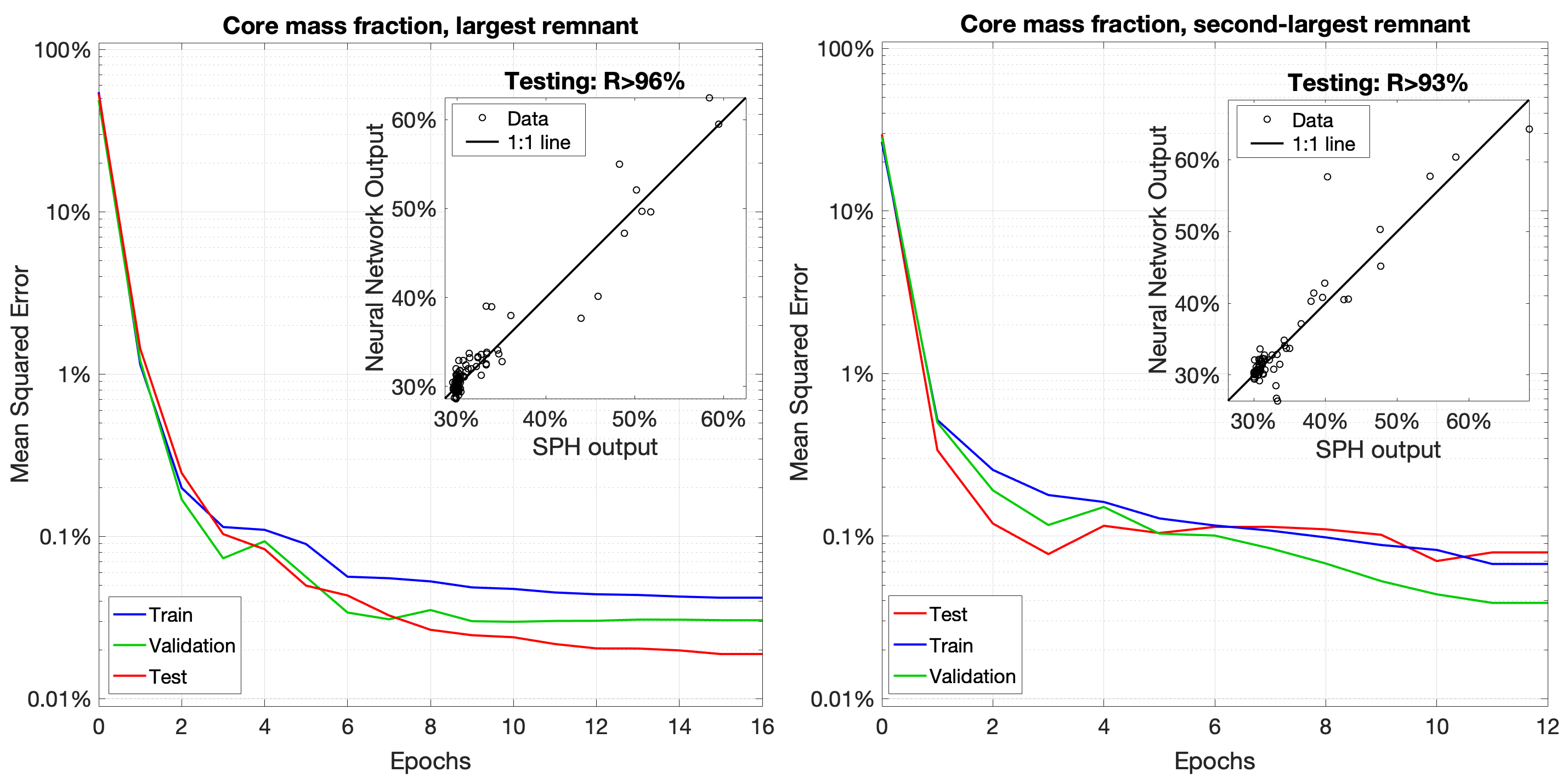
Figure 1: As the training proceeds, the mean squared errors (Equation 5) of the surrogate models of core mass fraction on the training (blue curves), validation (green curves) and testing (red curves) data sets decrease at each training epoch until convergence is reached. The performances of the surrogate models are quantified in terms of mean squared error (Equation 5) and correlation coefficient (Equation 6) at testing: {0.02%; $R>96\%$} and {0.08%; $R>93\%$} for the largest and second largest remnants, respectively. The two inset plots show the correlation between predictions by the neural networks and the corresponding SPH values in the testing data sets (open dots) and the 1:1 correlation line.

We use the same SPH data set as C19 and E20 to train two new surrogate models to predict the core mass fractions of the largest and second largest remnants. Each remnant’s core mass fraction is obtained by accounting for all material in the SPH simulations. This includes all gravitationally-bound material such as potential silicate vapour resulting from energetic collisions involving larger bodies or impact velocities. The core mass fractions of the target and projectile are termed $Z_{\mathrm{T}}$ and $Z_{\mathrm{P}}$, respectively. Their initial values are always equal to 30% .

For the first new surrogate model, we train, validate, and test a neural network using a data set with entries:

$$\{(M_{\mathrm{T}},~{}\gamma,~{}\theta_{\mathrm{coll}},~{}v_{\mathrm{coll}}/v_{\mathrm{esc}});Z_{\mathrm{L}}\},$$ (8)

where $Z_{\mathrm{L}}$ is the largest remnant’s core mass fraction. In the hit-and-run regime only, we train a second neural network to predict the core mass fraction of the second largest remnant. For this surrogate model, the data set has entries:

$$\{(M_{\mathrm{T}},~{}\gamma,~{}\theta_{\mathrm{coll}},~{}v_{\mathrm{coll}}/v_{\mathrm{esc}});Z_{\mathrm{S}}\},$$ (9)

where $Z_{\mathrm{S}}$ is the post-collision core mass fraction of the second largest remnant.

Following the approach described in C19 and E20, the training of the networks is performed on 70% of the overall data set. The rest of the data are split between a validation set (15%) and a testing set (15%) via random sampling without replacement. The optimal neural network architectures have 10 neurons in the hidden layer with an hyperbolic tangent sigmoid activation function (Equation 13 in C19). The inputs and targets are normalized in the range [-1, 1]. The regularization process (e.g., Girosi et al., 1995) has a strength equal to $5.48\times 10^{-6}$ and $3.80\times 10^{-5}$ for the $Z_{\mathrm{L}}$ and $Z_{\mathrm{S}}$ networks, respectively.

Each network is trained using the Levenberg-Marquardt algorithm described in Hagan et al. (1997). The learning dynamics (i.e., evolution of the mean squared error for training, validation, and testing at different epochs of training procedure) are plotted in Figure 1 for the largest and second largest remnants (left and right panels, respectively). At every training epoch, the weights of the networks are updated such that the mean squared error on the training data set gets progressively smaller. The mean squared errors converge in about 6 epochs for the surrogate model of the largest remnant and 4 for that of the second remnant.

Once trained, the predictive performance of the networks are quantified by the mean squared error (red curves in Figure 1, Equation 5) and correlation coefficient (box plots, Equation 6) on the testing dataset. The mean squared error at convergence is equal to about $2\times 10^{-4}$ with a correlation coefficient of above 96% for the largest remnant, and $8\times 10^{-4}$ with a correlation coefficient above 93% for the second largest remnant.

2.5 Accretion efficiencies of the core and the mantle

In order to track how the core mass fraction of a growing planet evolves through the giant impact phase of accretion, we split the change in mass from the target to the largest remnant into a core and mantle component:

$$M_{\mathrm{L}}-M_{\mathrm{T}}=\Delta M_{\mathrm{L}}^{\mathrm{c}}+\Delta M_{\mathrm{L}}^{\mathrm{m}},$$ (10)

where $\Delta M_{\mathrm{L}}^{\mathrm{c}}=M_{\mathrm{L}}^{\mathrm{c}}-M_{\mathrm{T}}^{\mathrm{c}}$ and $\Delta M_{\mathrm{L}}^{\mathrm{m}}=M_{\mathrm{L}}^{\mathrm{m}}-M_{\mathrm{T}}^{\mathrm{m}}$ are the changes in mass of the core and mantle of the largest remnant from the target as indicated by the superscripts “c” and “m”, respectively. Similarly, in the hit-and-run collision regime, we do the same for the change in mass from the projectile to the second largest remnant:

$$M_{\mathrm{S}}-M_{\mathrm{P}}=\Delta M_{\mathrm{S}}^{\mathrm{c}}+\Delta M_{\mathrm{S}}^{\mathrm{m}},$$ (11)

where $\Delta M_{\mathrm{S}}^{\mathrm{c}}=M_{\mathrm{S}}^{\mathrm{c}}-M_{\mathrm{P}}^{\mathrm{c}}$ and $\Delta M_{\mathrm{S}}^{\mathrm{m}}=M_{\mathrm{S}}^{\mathrm{m}}-M_{\mathrm{P}}^{\mathrm{m}}$ are defined similarly as the largest remnant case.

The remnant bodies after a giant impact may have different core mass fractions than either of the pre-impact bodies (i.e. target and projectile) or each other. For instance, a projectile may erode mantle material from the target in a hit-and-run collision, but during the same impact the target may accrete core material from the projectile. In order to quantify and study these possibilities, we define distinct accretion efficiencies for each remnants’ core ($\xi_{\mathrm{L}}^{\mathrm{c}}$ and $\xi_{\mathrm{S}}^{\mathrm{c}}$) and mantle ($\xi_{\mathrm{L}}^{\mathrm{m}}$ and $\xi_{\mathrm{S}}^{\mathrm{m}}$), so that, after dividing through by the projectile mass for normalization, the above expressions are transformed into:

$$\xi_{\mathrm{L}} =Z_{\mathrm{P}}\xi_{\mathrm{L}}^{\mathrm{c}}+(1-Z_{\mathrm{P}})\xi_{\mathrm{L}}^{\mathrm{m}},$$ (12)

$$\xi_{\mathrm{S}} =Z_{p}\xi_{\mathrm{S}}^{\mathrm{c}}+(1-Z_{\mathrm{P}})\xi_{\mathrm{S}}^{\mathrm{m}},$$ (13)

where we define the core and mantle component accretion efficiencies in the same manner as the overall accretion efficiencies of the remnant bodies:

$$\xi_{\mathrm{L}}^{\mathrm{c}} =\frac{M_{\mathrm{L}}^{\mathrm{c}}-M_{\mathrm{T}}^{\mathrm{c}}}{M_{\mathrm{P}}^{\mathrm{c}}}=\frac{Z_{\mathrm{L}}}{Z_{\mathrm{P}}}\xi_{\mathrm{L}}+\frac{Z_{\mathrm{L}}-Z_{\mathrm{T}}}{Z_{\mathrm{P}}}\frac{1}{\gamma},$$ (14)

$$\xi_{\mathrm{L}}^{\mathrm{m}} =\frac{M_{\mathrm{L}}^{\mathrm{m}}-M_{\mathrm{T}}^{\mathrm{m}}}{M_{\mathrm{P}}^{\mathrm{m}}}=\frac{1-Z_{\mathrm{L}}}{1-Z_{\mathrm{P}}}\xi_{\mathrm{L}}-\frac{Z_{\mathrm{L}}-Z_{\mathrm{T}}}{1-Z_{\mathrm{P}}}\frac{1}{\gamma},$$ (15)

$$\xi_{\mathrm{S}}^{\mathrm{c}} =\frac{M_{\mathrm{S}}^{\mathrm{c}}-M_{\mathrm{P}}^{\mathrm{c}}}{M_{\mathrm{P}}^{\mathrm{c}}}=\frac{Z_{\mathrm{S}}}{Z_{\mathrm{P}}}(1+\xi_{\mathrm{S}})-1,$$ (16)

$$\xi_{\mathrm{S}}^{\mathrm{m}} =\frac{M_{\mathrm{S}}^{\mathrm{m}}-M_{\mathrm{P}}^{\mathrm{m}}}{M_{\mathrm{P}}^{\mathrm{m}}}=\frac{1-Z_{\mathrm{S}}}{1-Z_{\mathrm{P}}}(1+\xi_{\mathrm{S}})-1,$$ (17)

where on the right-hand sides of Equations 14–17, we express the core and mantle accretion efficiencies in terms found in Table 1: the initial projectile-to-target mass ratio ($\gamma$), the overall accretion efficiencies of the remnants ($\xi_{\mathrm{L}}$ and $\xi_{\mathrm{S}}$), and the core mass fractions of the final bodies ($Z_{\mathrm{L}}$ and $Z_{\mathrm{S}}$).

3 Planetary differentiation model

After a giant impact, the surviving mantle of a remnant body is assumed to equilibrate with any accreted material, in a magma ocean produced by the energetic impact. This equilibration establishes the composition of the cooling magma ocean and also potentially involves dense Fe-rich metallic liquids that segregate to the core due to density differences. In this Section, we describe how the inefficient-accretion model of Section 2 is implemented into the planetary accretion and differentiation model published by Rubie et al. (2011, 2015, 2016). We direct the reader to the manuscripts by Rubie et al. for a more detailed description of the metal-silicate equilibration approach itself.

3.1 Identification of silicate and metallic reservoirs

In the flowchart of Figure 2, we outline the steps for identifying equilibrating silicate and metal reservoirs from surviving target and accreted projectile material in the remnants’ mantle. These steps are:

1. The classifier of collision type (Section 2.3) is used to determine the number of resulting bodies of a collision. In case there is only a single remnant (accretion or erosion regimes), the core of the projectile may be either accreted or obliterated. This is determined by looking at the sign of the largest remnant’s core accretion efficiency $\xi_{\mathrm{L}}^{\mathrm{c}}$.

2. If $\xi_{\mathrm{L}}^{\mathrm{c}}$ is positive and the event is not an hit-and-run collision, the metallic core of the projectile plunges into the target’s magma ocean turbulently entraining silicate liquid in a descending plume (Deguen et al., 2011; Rubie et al., 2003). The plume’s silicate content increases as the plume expands with increasing depth. This determines the volume fraction of metal $\phi_{\mathrm{met}}$ (Rubie et al., 2015):

   $$\phi_{\mathrm{met}}=\bigg{(}1+\frac{\alpha z}{r_{0}}\bigg{)}^{-3}$$ (18)

   where $\alpha=0.25$ (Deguen et al., 2011), $r_{0}$ is the initial radius of the projectile’s core and $z$ is depth in the magma ocean. Equation 18 allows estimating the mass fraction of the embryo’s mantle material that is entrained as silicate liquid since the volume of the descending projectile core material is known. Following chemical equilibration during descent, any resulting metal is added to the proto-core and the equilibrated silicate is mixed with the fraction of the mantle that did not equilibrate to produce a compositionally homogeneous mantle (Rubie et al., 2015), under the assumption of vigorous mixing due to mantle convection.

3. If $\xi_{\mathrm{L}}^{\mathrm{c}}$ is negative, the target’s core and mantle are eroded and the projectile is obliterated. For this case,

4. For hit-and-run collisions, the projectile survives accretion and becomes the second remnant of the collision. There may be mass transfer between the colliding bodies as predicted using the surrogate models of Section 2.2 and Section 2.4.

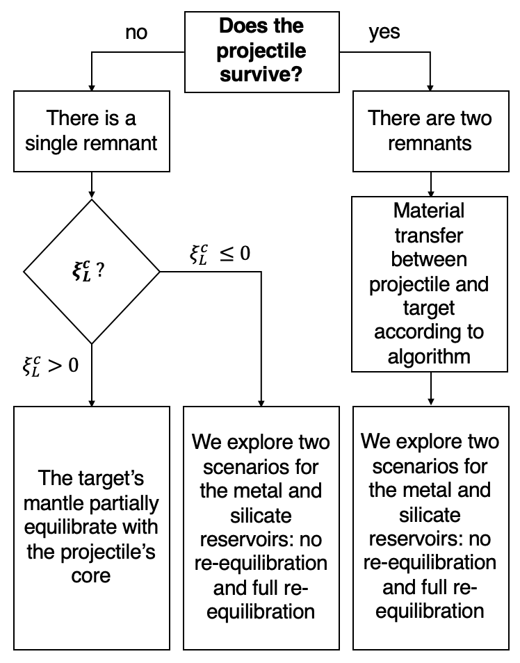
Figure 2: In the planetary differentiation model, we first identify the interacting reservoirs of the resulting bodies of a collision (the top three rows of this flowchart) using the surrogate model described in Section 2. The information is then passed to the metal-silicate equilibration model described in Section 3 (bottom row).

3.2 Mass balance

After each , there is re-equilibration between any interacting silicate-rich and metallic phases in the remaining bodies, which ultimately determines the compositions of the mantle and core. The volume of interacting material is determined as described in Section 3.1 and shown schematically in Figure 2. The planetary differentiation model tracks the partitioning of elements in the post-impact magma ocean between a silicate phase, which is modeled as a silicate-rich phase mainly composed of SiO₂, Al₂O₃, MgO, CaO, FeO, and NiO, and a metallic phase, which is modeled as a metal reservoir mainly composed of Fe, Si, Ni, and O. Both the silicate-rich and metal phases include the minor and trace elements: Na, Co, Nb, Ta, V, Cr, Pt, Pd, Ru, Ir, W, Mo, S, C, and H.

The identified silicate-rich and metal phases equilibrate as described by the following mass balance equation:

$$\begin{split}\mathrm{Silicate~{}Liquid~{}}(1)+\mathrm{Metal~{}Liquid~{}}(1)\\ \Longrightarrow\mathrm{Silicate~{}Liquid~{}}(2)+\mathrm{Metal~{}Liquid~{}}(2)\end{split}$$ (19)

where the flag “1” indicates the system before equilibration and the flag “2” indicates the system which is equilibrated under the new thermodynamic conditions of the resulting bodies of a collision. Thus, all equilibrating atoms are conserved and the oxygen fugacity of the reaction is set implicitly.

In the chemical equilibrium of Equation 19, the partitioning of the elements into the core and mantle is controlled by the three parameters of the model: pressure $P_{e}$, temperature $T_{e}$, and oxygen fugacity $f_{O_{2}}$ of metal-silicate equilibration. These are in turn a function of the type of collision and its accretion efficiencies (Section 2.5), which control how the reservoirs of the target and projectile interact. In the following, the treatment of these thermodynamic properties in the context of inefficient accretion and equilibration is described.

3.2.1 Equilibration pressure and temperature

Following each event , the silicate-rich and the iron-rich reservoirs are assumed to equilibrate at a pressure $P_{\mathrm{e}}$ which is a constant fraction $f_{\mathrm{P}}$ of the embryos’ evolving core–mantle boundary pressure $P_{\mathrm{CMB}}$,

$$P_{\mathrm{e}}=f_{\mathrm{P}}P_{\mathrm{CMB}},$$ (20)

and the equilibration temperature $T_{\mathrm{e}}$ is forced to lie midway between the peridotite liquidus and solidus at the equilibration pressure $P_{\mathrm{e}}$ (e.g., Rubie et al., 2015).

The pressure $P_{\mathrm{e}}$ defined in Equation 20 is a simplified empirical parameter which averages the equilibration pressures for different types of impact events, and the constant $f_{\mathrm{P}}$ is a proxy for the average depth of impact-induced magma oceans. Here, we adopt a value $f_{\mathrm{P}}=0.7$ for all the accretion events, consistently with the findings by de Vries et al. (2016), which studied the pressure and temperature conditions of metal-silicate equilibration, after each impact, as Earth-like planets accrete.

For each of the resulting bodies, we determine the pressure $P_{\mathrm{CMB}}$ by using Equation 2.73 in Turcotte & Schubert (2002). The radial position of the core-mantle boundary is computed by using the approximation that an embryo is a simple two-layer sphere of radius $R$ consisting of a core of density $\rho_{\mathrm{c}}$ and radius $R_{\mathrm{c}}$ surrounded by a mantle of thickness ($R-R_{\mathrm{c}}$):

$$R_{\mathrm{c}}=\left(\frac{\rho-\rho_{\mathrm{m}}}{\rho_{\mathrm{c}}-\rho_{\mathrm{m}}}\right)^{\frac{1}{3}}R$$ (21)

where the embryo’s mean density $\rho$ is provided by the density-mass relationship introduced in E20 . Assuming a mantle density $\rho_{\mathrm{m}}=0.4~{}\rho_{\mathrm{c}}$ (), the core density $\rho_{\mathrm{c}}$ is equal to

$$\rho_{\mathrm{c}}=\frac{5}{2}\rho\left(1-\frac{3}{5}Z\right)$$ (22)

where $Z$ is the embryo’s core mass fraction as predicted by the surrogate models in Section 2.4.

3.2.2 Oxygen fugacity

The oxygen fugacity $f_{\mathrm{O_{2}}}$ determines the redox conditions for geologic chemical reactions. It is a measure of the effective availability of oxygen for redox reactions, and it dictates the oxidation states of cations like iron that have multiple possible valence states. For oxygen-poor compositions, oxygen fugacity is a strong function of temperature because the concentration of Si in the metal strongly increases with temperature which increases the concentration of FeO in the silicate. For more oxidized compositions, both Si and O dissolve in the metal, and oxygen fugacity is a much weaker function of temperature than in the case of more reduced bulk compositions.

The major benefit of the mass balance approach to modeling metal-silicate equilibration as described in Section 3.2 is that the oxygen fugacity does not need to be assumed (as is done in most core formation models), but it is determined directly from the compositions of equilibrated metal and silicate (Equation 19). The oxygen fugacity is defined as the partition coefficient of iron between metal and silicate computed relative to the iron-wüstite buffer (IW, the oxygen fugacity defined by the equilibrium 2Fe + O₂ = 2 FeO):

$$\log{f_{\mathrm{O_{2}}}}(\Delta\mathrm{IW})=2\log{\left(\frac{X_{\mathrm{FeO}}^{\mathrm{Mw}}}{X_{\mathrm{Fe}}^{\mathrm{met}}}\right)}$$ (23)

4 Inefficient accretion versus perfect merging: single impact events

Figure 3: Relative difference between the core mass fractions of the largest remnant (left panel) and second remnant (right panel) and those of the parent bodies (the target’s and projectile’s, respectively) for a collision with $M_{\mathrm{T}}=$0.1\text{\,}\mathrm{M_{\oplus}}$$ and projectile-to-target mass ratio $\gamma=0.7$ happening at different impact angles $\theta_{coll}$ and impact velocities $v_{coll}$ (in units of escape velocity $v_{esc}$). Each point represents a different collision scenario in which the two bodies collide at different impact angles and velocities. The black curves define the different accretion regimes predicted using the classifier of Section 2.3. For comparison, the perfect-merging model predicts that the outcome of the collision is a single larger embryo with core mass fraction equal to that of the target (i.e. relative difference equal to zero) and no second remnant exists.

Here, we compare the predictions of the perfect-merging model and the inefficient-accretion model of Section 2 for the case study of a single giant impact between a target of mass $M_{\mathrm{T}}=$0.1\text{\,}\mathrm{M_{\oplus}}$$ and a projectile of mass $M_{\mathrm{P}}=0.7M_{\mathrm{T}}$. For the two models, we analyze the core mass fraction (Section 4.1), accretion efficiencies of the cores and the mantles (Section 4.2), pressure, temperature, and oxygen fugacity of metal-silicate equilibration of the resulting bodies (Section 4.3).

4.1 Core mass fraction

4.2 Accretion efficiency

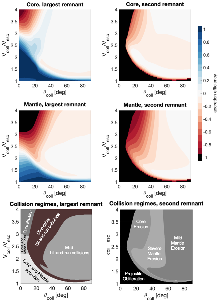
Figure 4: Accretion efficiency of the core (first row) and mantle (second row) for the largest remnant (left panels) and second largest remnant (right panels) and corresponding collision regimes as predicted by the inefficient-accretion model (third row) for a collision with $M_{\mathrm{T}}=$0.1\text{\,}\mathrm{M_{\oplus}}$$ and projectile-to-target mass ratio $\gamma=0.7$, for different impact angles $\theta_{coll}$ and impact velocities $v_{coll}$ (in units of escape velocity $v_{esc}$).

(Rubie et al., 2015). For a collision between a target of mass $M_{\mathrm{T}}=$0.1\text{\,}\mathrm{M_{\oplus}}$$ and a projectile of mass $M_{\mathrm{P}}=0.7M_{\mathrm{T}}$, the perfect-merging model predicts that the projectile’s core plunges into the target mantle and that the entire projectile’s mantle is accreted ($\xi_{\mathrm{L}}^{\mathrm{m}}=\xi_{\mathrm{L}}^{\mathrm{c}}=1$), for every combination of impact angle and velocity.

In the parameter space of impact angle and impact velocity, we identify five collision regimes according to the core and mantle’s accretion efficiencies of the largest remnant. These are described in the bottom-left panel of Figure 4 and defined as:

1. Core and mantle accretion occurs when $\xi_{\mathrm{L}}^{\mathrm{c}}\geq$ 0 and $\xi_{\mathrm{L}}^{\mathrm{m}}\geq$ 0. the projectile plunges into the target and gets accreted.

2. Core accretion with loss of mantle material occurs when $\xi_{\mathrm{L}}^{\mathrm{c}}\geq$ 0 and $\xi_{\mathrm{L}}^{\mathrm{m}}<$ 0. the projectile’s core plunges into the target and gets accreted.

3. Core erosion occurs when $\xi_{\mathrm{L}}^{\mathrm{c}}<0$. The target’s mantle is catastrophically disrupted and core erosion may also occur. The largest remnant has a larger core mass fraction than the target (Figure 3). the projectile is obliterated.

4. Mild hit-and-run collisions occur when $\xi_{\mathrm{L}}^{\mathrm{c}}\in[-0.1,~{}0.1]$ and $\xi_{\mathrm{L}}^{\mathrm{m}}\in[-0.1,~{}0.1]$. The target’s core does not gain or lose substantial mass, while the target’s mantle may lose some mass depending on the impact velocity. The bulk projectile escapes accretion and becomes the second remnant. Substantial debris production may occur.

For the second remnant, we identify four collision regimes which are described in the bottom-right panel of Figure 4:

1. Mild mantle erosion occurs when $\xi_{\mathrm{S}}^{\mathrm{c}}\in[-0.1,~{}0.1]$ and $\xi_{\mathrm{S}}^{\mathrm{m}}\in[-0.1,~{}0.1]$. At high impact angle, the geometry of the impact prevents almost any exchange of mass between the target and the projectile.

2. Severe mantle erosion occurs when $\xi_{\mathrm{S}}^{\mathrm{c}}\in[-0.1,~{}0.1]$ and $\xi_{\mathrm{S}}^{\mathrm{m}}<-0.1$. The second remnant has a less massive mantle compared to the projectile, while it retains its core mostly intact.

3. Core erosion occurs when $\xi_{\mathrm{S}}^{\mathrm{c}}<$-0.1. The second remnant’s core mass fraction is strongly enhanced with respect to that of the projectile. In disruptive hit-and-run collisions, the energy of the impact may be high enough to erode some core material.

4. Projectile obliteration occurs when $\xi_{\mathrm{S}}=\xi_{\mathrm{S}}^{\mathrm{c}}=\xi_{\mathrm{S}}^{\mathrm{m}}=-1$. No second remnant exists, as the projectile is either accreted or completely disrupted.

4.3 Pressure, temperature and oxygen fugacity

The equilibration conditions of planets resulting from inefficient accretion (due to the stripping of mantle and core materials) will differ from those produced by the perfect-merging model. In Figure 5 we show the difference in equilibration conditions for a single impact scenario (the same impact scenario as the previous sections); . The relative differences in the equilibration results are computed with respect to the perfect-merging values as

$$\delta X=\frac{X_{\mathrm{inefficient~{}accretion}}-X_{\mathrm{perfect~{}merging}}}{X_{\mathrm{perfect~{}merging}}}\times$100\text{\,}\mathrm{\char 37\relax}$,$$ (24)

where $X$ indicates one of the thermodynamic metal-silicate equilibration parameters: pressure, temperature, or oxygen fugacity of metal-silicate equilibration for an embryo with initial $X_{\mathrm{Fe}}^{\mathrm{met}}=0.99$. Positive values of $\delta[\log{f_{\mathrm{O_{2}}}}]$ indicate that the metal-silicate equilibration in the resulting body occurs at more chemically reduced conditions than in the planet from the perfect-merging model because of lower equilibration temperatures, while negative values of $\delta[\log{f_{\mathrm{O_{2}}}}]$ indicate less chemically reduced conditions.

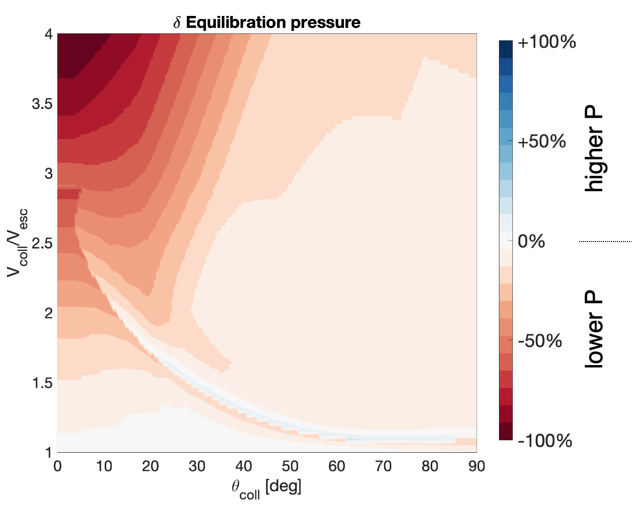
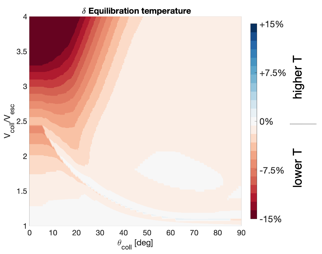
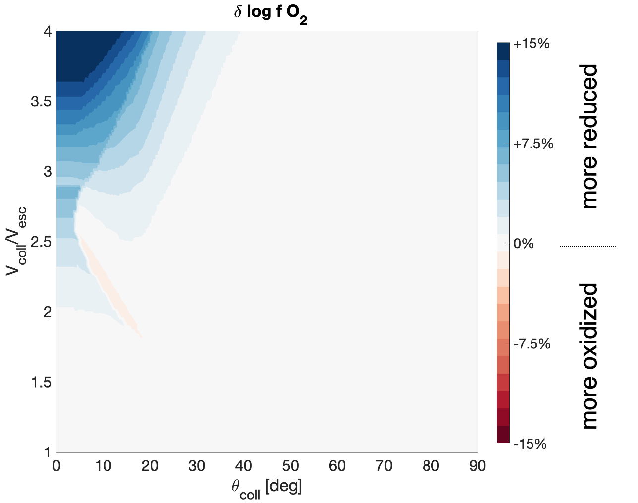
Figure 5: Relative difference (Equation 24) between the predicted values of pressure, temperature, and oxygen fugacity of metal-silicate equilibration of the largest remnant from the inefficient-accretion model and those of the resulting body from the perfect-merging model (Equation 24), for the same collision of Figure 3 and 4. The colliding embryos have initial molar fraction of iron in the metal phase $X_{\mathrm{Fe}}^{\mathrm{met}}=0.99$. .

5 Inefficient accretion versus perfect merging: N-body simulations

In this Section, we investigate how planetary differentiation is affected by inefficient accretion during the end-stage of terrestrial planet formation. In contrast to Section 4, in which we investigate the case study of a single giant impact, here we use the core-mantle differentiation model to interpret the results of the N-body simulations of accretion by E20 which model the evolution of hundreds of Moon-to-Mars-sized embryos as they orbit the Sun and collide to form the terrestrial planets. The goal of our analysis, however, is not to reproduce the solar system terrestrial planets, but to investigate whether or not the perfect-merging and inefficient-accretion models produce significantly different predictions for the terrestrial planets’ final properties .

5.1 Initial mass and composition of the embryos

We use the data set of N-body runs performed in E20 and test the effects of the two collision models under a single equilibration model. The dataset consists of 16 simulations that use the more realistic treatment of collisions (inefficient-accretion model) and, in addition, 16 control simulations where collisions are taken to be fully accretionary (perfect-merging model). All the simulations were obtained with the mercury6 N-body code (Chambers, 1999). For the inefficient-accretion model, E20 use the code library collresolve (Emsenhuber & Cambioni, 2019). Each N-body simulation begins with 153–158 planetary embryos moving in a disk with surface density similar to that for solids in a minimum mass solar nebula (Weidenschilling, 1977). As in Chambers (2001), two initial mass distributions are examined: approximately uniform masses, and a bimodal distribution with a few large (i.e., Mars-sized) and many small (i.e., Moon-sized) bodies. The embryos in the simulations 01–04 all have the same initial mass . In simulations 11–14, the embryos have their initial mass proportional to the local surface density of solids. In simulations 21–24, the initial mass distribution is bimodal and the two populations of embryos are characterized by bodies with the same mass; . In simulations 31–34, the initial mass distribution is also bimodal but the bodies have mass proportional to the local surface density.

The compositions of the initial embryos are set by the initial oxygen fugacity conditions of the early solar system materials which are defined as a function of heliocentric distance. Among the models of early solar system materials that have heritage in the literature, we adopt the model by Rubie et al. (2015), whose parameters were refined through least squares minimization to obtain an Earth-like planet with mantle composition close to that of the Bulk Silicate Earth. Accretion happens from two distinct reservoirs of planet-forming materials: one of reduced material in the inner solar system $<0.95\text{\,}\mathrm{au}$, with the fraction of iron dissolved in metal equal to $0.99$ and fraction of available silicon dissolved in the metal equal to $0.20$. Exterior to that, no dissolved silicon is present in the metal and the proportion of Fe in metal decreases linearly until a value of $0.11$ is reached at $2.82\text{\,}\mathrm{au}$. Beyond 2.82 au, the iron metal fraction linearly decreases and reaches about zero at $6.8\text{\,}\mathrm{au}$

In sets 01–04 and 21–24, the initial mass , so the number density of embryos scales with the surface density. In sets 11–14 and 31–34, the initial embryos’ masses scale with the local surface density; the spacing between embryos is independent of the surface density, but the heliocentric distance between them gets smaller as distance increases, hence the number density of the embryos increases with heliocentric distance. This means that the simulations 11–14 and 31–34 are initialized with most of the embryos forming farther from the Sun than those in simulations 01–04 and 21–24. Following the model by Rubie et al. (2015), this implies that most of the embryos in simulations 11–14 and 31–34 form with initial core mass fractions .

5.2 Working assumptions

1. The N-body simulations of E20 are based on the assumption that the bodies are not spinning prior to each collision and are not spinning afterwards. We acknowledge that this approximation violates the conservation of angular momentum and that collisions between spinning bodies would alter accretion behavior (e.g., Agnor et al., 1999).

2. In the N-body simulations with inefficient accretion by E20, only the remnants whose mass is larger than $1\text{\times}{10}^{-3}\text{\,}\mathrm{M_{\oplus}}$ are considered.

3. As the embryos evolve during accretion through collisions, their core mass fractions can evolve to be different from 30%, which is the core mass fraction of the SPH colliding bodies that were used to train the surrogate models in Section 2.4. For this reason, in the analysis of the N-body simulations we make the approximation that the core mass fraction of each collision remnant is equal to

   $$Z\approx(Z^{*}-30\%)+Z_{0}$$ (25)

   where $Z^{*}$ is the core mass fraction of the remnant as predicted by the surrogate model of Section 2.4, and $Z_{0}$ is the metal fraction of the parent body as computed by the core-mantle differentiation model.

5.3 Results: Core mass fraction

To compare the effect of the two accretion model assumptions (inefficient accretion and perfect merging) for planets in the N-body simulations, we examine the final core mass fractions.

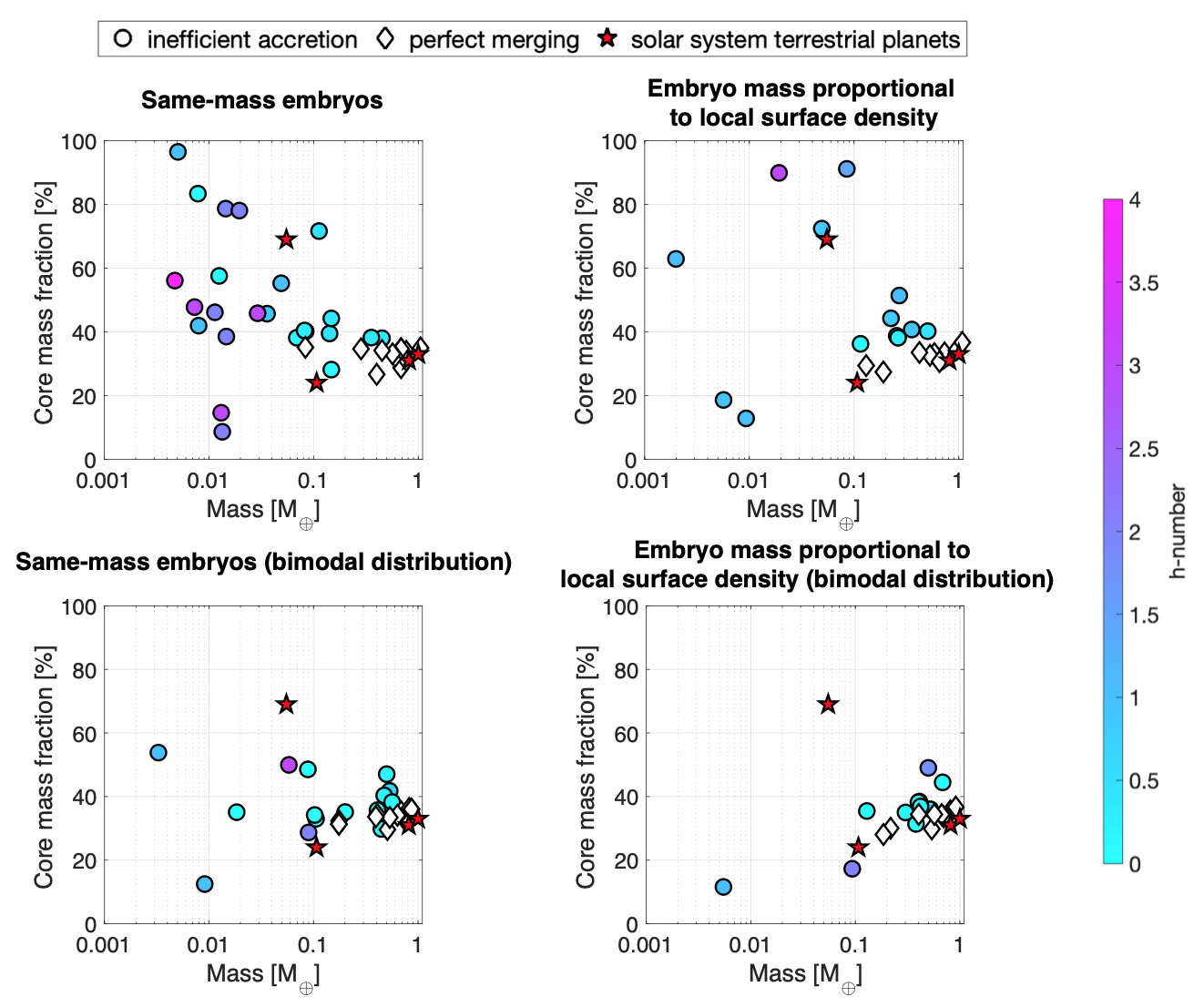
Figure 6: N-body results by the inefficient-accretion model (dots) and the perfect-merging model (diamonds) in terms of the final planets’ core mass fraction as function of the final planetary mass and different initial mass distributions for the embryos. . The red stars show the core mass fractions of the solar system terrestrial planets.

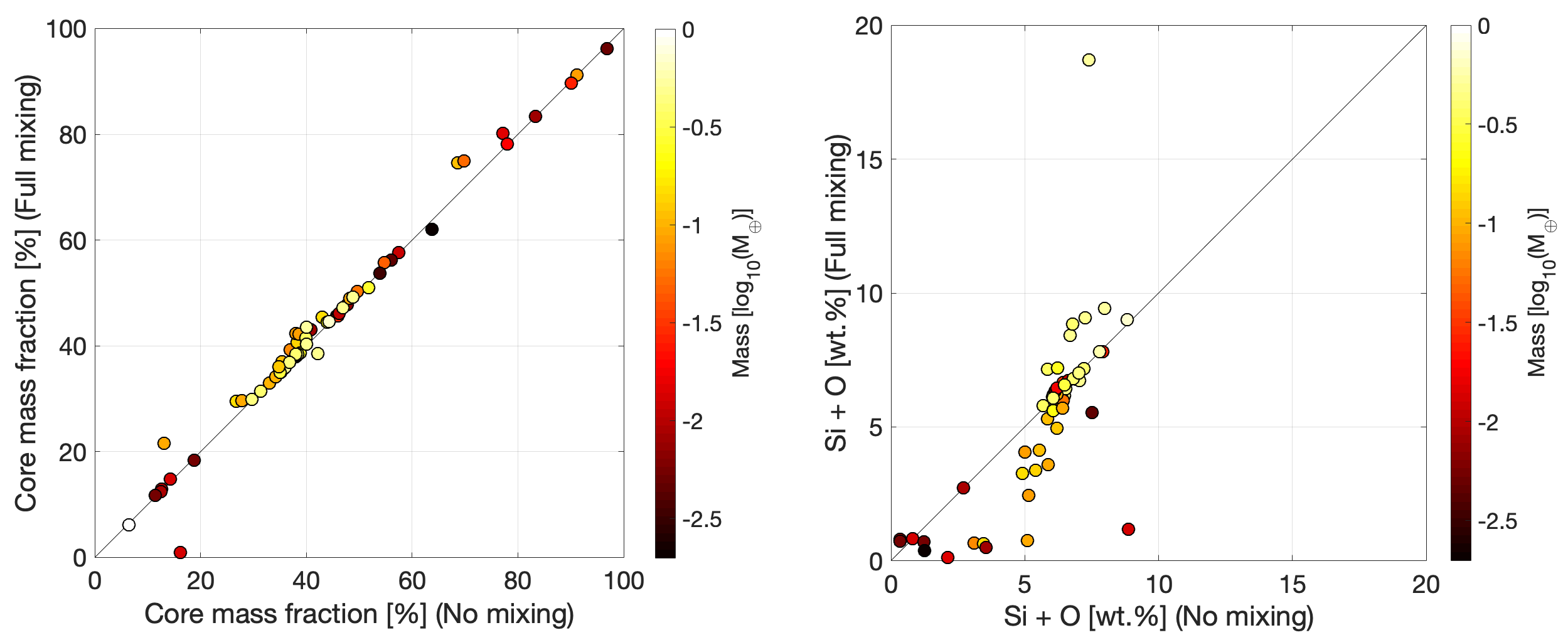
Figure 7: Left panel: core mass fraction of the terrestrial planets obtained in all the N-body simulations from E20  assuming that full mixing and re-equilibration occur at the core-mantle boundary (vertical axis) or no re-equilibration occurs (horizontal axis) in hit-and-run and erosive collisions. Right panel: same as the left panel, but for the concentration of Si and O in the core of the terrestrial planets. The data points are color coded in terms of the planets’ masses (logarithmic scale).

Figure 6 is a plot of the core mass fraction of the final planets as a function of planetary mass as determined by the perfect-merging model (open diamonds) and the inefficient-accretion model (dots). Each of the four subpanels of Figure 6 plots one of the four groups of N-body simulations (01–04, 11–14, 21–24, 31–34) described in Section 5.1. Each subpanel shows the results from all the four N-body simulations of the correspondent group. The inefficient-accretion results are color-coded in terms of their $h$-number, which measures how many hit-and-run collisions an embryo experienced during the accretion simulation . If the collision event is a merger, the largest remnant’s $h$-number is equal to the mass average of the target’s and projectile’s $h$-numbers. If the event is a hit-and-run collision, the second remnant’s $h$-number is increased by 1, . We also plot the estimated values for the core mass fractions of the inner solar system terrestrial bodies as red stars: $Z_{\mathrm{Earth}}=$33\text{\,}\mathrm{\char 37\relax}$$ , $Z_{\mathrm{Venus}}=$31\text{\,}\mathrm{\char 37\relax}$$, $Z_{\mathrm{Mars}}=$24\text{\,}\mathrm{\char 37\relax}$$, $Z_{\mathrm{Mercury}}=$69\text{\,}\mathrm{\char 37\relax}$$ (Sorokhtin et al., 2011; Rubie et al., 2015; Helffrich, 2017; Hauck et al., 2013, respectively).

remnants with core mass fractions above 40% are generally found to have relatively high $h$-numbers, meaning that they survived multiple hit-and-run collisions.

As discussed in E20, the initial mass of the embryos influences the dynamical environment and thus imparts a change in the degree of mixing between feeding zones in the planetary disk. This is found to affect the spread in core mass fraction of the smaller embryos. The simulations that produced the results in the top panels of Figure 6 were initialized with embryos of similar mass. As a result, these simulations are characterized by a predominance of collisions between similar-mass bodies which tend to result in more hit-and-run collisions (Asphaug, 2010; Gabriel et al., 2020). many of the less massive planets are the “runners” from hit-and-run collisions (blue and magenta colored points), which managed to escape accretion onto the larger bodies but lost mantle material in the process, an effect predicted in Asphaug & Reufer (2014). This also explains why remnants with high $h$-numbers tend to also have higher core mass fractions.

We also observe that the spread in core mass fraction in small bodies depends also on the heliocentric distance at which they form. Adopting the model for early solar system materials by Rubie et al. (2015), the embryos that form farther than $0.95\text{\,}\mathrm{a}\mathrm{u}$ have an initial core mass fraction lower than 30% due to oxidation of metallic iron by water. This explains the presence of a few small embryos with core mass fraction lower than 30%.

.

5.4 Statistics of planetary diversity

Table 2: Average value and range of the values of core mass fractions for the two populations of Inefficient-Accretion (IA) planets with M$<$0.1 M_⊕ and M$>$0.1 M_⊕. The symbols $\bar{Z}$ and $\Delta Z$ indicate the average core mass fraction of the population and its range, respectively. For reference, the Perfect-Merging (PM) planets have $\bar{Z}_{PM}~{}\approx$ $33\text{\,}\%$ and $\Delta Z_{PM}~{}\approx$ $8\text{\,}\%$.

Sims	$\bar{Z}_{IA}$ (M $<$ 0.1 M⊕)	$\Delta Z_{IA}$ (M $<$ 0.1 M⊕)	$\bar{Z}_{IA}$ (M $>$ 0.1 M⊕)	$\Delta Z_{IA}$ (M $>$ 0.1 M⊕)
01–04	51%	88%	40%	16%
11–14	57%	78%	41%	16%
21–24	38%	41%	37%	17%
31–34	15%	6%	38%	18%

5.5 Effect of debris re-accretion

(e.g., Stewart & Leinhardt, 2009; Kokubo & Genda, 2010; Chambers, 2013; Quintana et al., 2016)

5.6 Future work

6 Conclusions

In this work, neural networks trained on giant impact simulations have been implemented in a core-mantle differentiation model coupled with N-body orbital dynamical evolution simulations to study the effect of inefficient accretion on planetary differentiation and evolution. We make a comparison between the results of the neural-network model (“inefficient accretion”) and those obtained by treating all collisions unconditionally as mergers with no production of debris (“perfect merging”).

For a single collision scenario between two planetary embryos, we find that the assumption of perfect merging overestimates the resulting bodies’ mass and thus their equilibration pressure and temperature. Assuming that the colliding bodies have oxygen-poor bulk compositions, the inefficient-accretion model produces a wider range of oxidation states that depends intimately on the impact velocity and angle; mass loss due to inefficient accretion leads to more reduced oxygen fugacities of metal-silicate equilibration because of the strong temperature dependence at low oxygen fugacities.

To investigate the cumulative effect of giant impacts on planetary differentiation, we use a core-mantle differentiation model to post-process the results of N-body simulations obtained in E20, where terrestrial planet formation was modeled with both perfect merging and inefficient accretion. . In contrast, both models provide similar predictions for planets more massive than $\approx 0.1\text{\,}\mathrm{M_{\oplus}}$, This is consistent with previous studies that successfully reproduced Earth’s Bulk Silicate composition using the results from N-body simulations with perfect merging (Rubie et al., 2015, 2016). We therefore suggest that an inefficient-accretion model is necessary to accurately track compositional evolution in terrestrial planet formation

Finally, the value of oxygen fugacity of metal-silicate equilibration is known to influence the post-accretion evolution of rocky planets’ atmospheres (e.g., Zahnle et al., 2007; Armstrong et al., 2019; Zahnle et al., 2020). Improving the realism of planet formation models with realistic collision models therefore becomes crucial not only for understanding how terrestrial embryos accrete, but also to make testable predictions of how some of them may evolve from magma-ocean planets to potentially habitable worlds.

References

- Agnor & Asphaug (2004) Agnor, C., & Asphaug, E. 2004, ApJ, 613, L157, doi: 10.1086/425158
- Agnor et al. (1999) Agnor, C. B., Canup, R. M., & Levison, H. F. 1999, Icarus, 142, 219, doi: 10.1006/icar.1999.6201
- Armstrong et al. (2019) Armstrong, K., Frost, D. J., McCammon, C. A., Rubie, D. C., & Boffa Ballaran, T. 2019, Science, 365, 903, doi: 10.1126/science.aax8376
- Asphaug (2010) Asphaug, E. 2010, Chemie der Erde / Geochemistry, 70, 199, doi: 10.1016/j.chemer.2010.01.004
- Asphaug et al. (2006) Asphaug, E., Agnor, C. B., & Williams, Q. 2006, Nature, 439, 155, doi: 10.1038/nature04311
- Asphaug & Reufer (2014) Asphaug, E., & Reufer, A. 2014, NatGeo, 7, 564, doi: 10.1038/ngeo2189
- Bonsor et al. (2015) Bonsor, A., Leinhardt, Z. M., Carter, P. J., et al. 2015, Icarus, 247, 291, doi: 10.1016/j.icarus.2014.10.019
- Burger et al. (2020) Burger, C., Bazsó, Á., & Schäfer, C. M. 2020, A&A, 634, A76, doi: 10.1051/0004-6361/201936366
- Cambioni et al. (2019) Cambioni, S., Asphaug, E., Emsenhuber, A., et al. 2019, ApJ, 875, 40, doi: 10.3847/1538-4357/ab0e8a
- Carter et al. (2015) Carter, P. J., Leinhardt, Z. M., Elliott, T., Walter, M. J., & Stewart, S. T. 2015, ApJ, 813, 72, doi: 10.1088/0004-637X/813/1/72
- Chambers (1999) Chambers, J. E. 1999, MNRAS, 304, 793, doi: 10.1046/j.1365-8711.1999.02379.x
- Chambers (2001) —. 2001, Icarus, 152, 205, doi: 10.1006/icar.2001.6639
- Chambers (2013) —. 2013, Icarus, 224, 43, doi: 10.1016/j.icarus.2013.02.015
- Clement et al. (2019) Clement, M. S., Raymond, S. N., & Kaib, N. A. 2019, AJ, 157, 38, doi: 10.3847/1538-3881/aaf21e
- Dahl & Stevenson (2010) Dahl, T. W., & Stevenson, D. J. 2010, Earth and Planetary Science Letters, 295, 177, doi: 10.1016/j.epsl.2010.03.038
- de Vries et al. (2016) de Vries, J., Nimmo, F., Melosh, H. J., et al. 2016, Progress in Earth and Planetary Science, 3, 7, doi: 10.1186/s40645-016-0083-8
- Deguen et al. (2011) Deguen, R., Olson, P., & Cardin, P. 2011, EPSL, 310, 303, doi: 10.1016/j.epsl.2011.08.041
- Dwyer et al. (2015) Dwyer, C. A., Nimmo, F., & Chambers, J. E. 2015, Icarus, 245, 145, doi: 10.1016/j.icarus.2014.09.010
- Emsenhuber & Asphaug (2019) Emsenhuber, A., & Asphaug, E. 2019, ApJ, 875, 95, doi: 10.3847/1538-4357/ab0c1d
- Emsenhuber & Cambioni (2019) Emsenhuber, A., & Cambioni, S. 2019, collresolve, 1.1, Zenodo, doi: 10.5281/zenodo.3560892
- Emsenhuber et al. (2020) Emsenhuber, A., Cambioni, S., Asphaug, E., et al. 2020, ApJ, 691, 6, doi: 10.3847/1538-4357/ab6de5
- Fischer et al. (2017) Fischer, R. A., Campbell, A. J., & Ciesla, F. J. 2017, Earth and Planetary Science Letters, 458, 252, doi: 10.1016/j.epsl.2016.10.025
- Frost et al. (2010) Frost, D. J., Asahara, Y., Rubie, D. C., et al. 2010, Journal of Geophysical Research (Solid Earth), 115, B02202, doi: 10.1029/2009JB006302
- Gabriel et al. (2020) Gabriel, T. S. J., Jackson, A. P., Asphaug, E., et al. 2020, ApJ, 892, 40, doi: 10.3847/1538-4357/ab528d
- Genda et al. (2017) Genda, H., Fujita, T., Kobayashi, H., et al. 2017, Icarus, 294, 234, doi: 10.1016/j.icarus.2017.03.009
- Gessmann et al. (1999) Gessmann, C. K., Rubie, D. C., & McCammon, C. A. 1999, Geochim. Cosmochim. Acta, 63, 1853, doi: 10.1016/S0016-7037(99)00059-9
- Girosi et al. (1995) Girosi, F., Jones, M., & Poggio, T. 1995, Neural computation, 7, 219
- Hagan et al. (1997) Hagan, M. T., Demuth, H. B., & Beale, M. 1997, Neural network design (PWS Publishing Co.)
- Hauck et al. (2013) Hauck, S. A., Margot, J.-L., Solomon, S. C., et al. 2013, Journal of Geophysical Research (Planets), 118, 1204, doi: 10.1002/jgre.20091
- Helffrich (2017) Helffrich, G. 2017, Progress in Earth and Planetary Science, 4, 24, doi: 10.1186/s40645-017-0139-4
- Holsapple (1994) Holsapple, K. 1994, Planetary and Space Science, 42, 1067, doi: https://doi.org/10.1016/0032-0633(94)90007-8
- Holsapple & Housen (1986) Holsapple, K. A., & Housen, K. R. 1986, Mem. Soc. Astron. Italiana, 57, 65
- Housen & Holsapple (1990) Housen, K. R., & Holsapple, K. A. 1990, Icarus, 84, 226, doi: https://doi.org/10.1016/0019-1035(90)90168-9
- Jacobson et al. (2017) Jacobson, S. A., Rubie, D. C., Hernlund, J., Morbidelli, A., & Nakajima, M. 2017, EPSL, 474, 375, doi: 10.1016/j.epsl.2017.06.023
- Kegler et al. (2008) Kegler, P., Holzheid, A., Frost, D. J., et al. 2008, Earth and Planetary Science Letters, 268, 28, doi: 10.1016/j.epsl.2007.12.020
- Kobayashi et al. (2019) Kobayashi, H., Isoya, K., & Sato, Y. 2019, ApJ, 887, 226, doi: 10.3847/1538-4357/ab5307
- Kokubo & Genda (2010) Kokubo, E., & Genda, H. 2010, ApJ, 714, L21, doi: 10.1088/2041-8205/714/1/L21
- Leinhardt & Stewart (2012) Leinhardt, Z. M., & Stewart, S. T. 2012, ApJ, 745, 79, doi: 10.1088/0004-637X/745/1/79
- Lock & Stewart (2019) Lock, S. J., & Stewart, S. T. 2019, Science Advances, 5, eaav3746, doi: 10.1126/sciadv.aav3746
- Mann et al. (2009) Mann, U., Frost, D. J., & Rubie, D. C. 2009, Geochim. Cosmochim. Acta, 73, 7360, doi: 10.1016/j.gca.2009.08.006
- Melosh (2007) Melosh, H. J. 2007, \maps, 42, 2079, doi: 10.1111/j.1945-5100.2007.tb01009.x
- Monaghan (1992) Monaghan, J. J. 1992, ARA&A, 30, 543, doi: 10.1146/annurev.aa.30.090192.002551
- Nakajima & Stevenson (2016) Nakajima, M., & Stevenson, D. J. 2016, in Lunar and Planetary Science Conference, Lunar and Planetary Science Conference, 2053
- O’Brien et al. (2006) O’Brien, D. P., Morbidelli, A., & Levison, H. F. 2006, Icarus, 184, 39, doi: 10.1016/j.icarus.2006.04.005
- Palme & O’Neill (2003) Palme, H., & O’Neill, H. S. C. 2003, Treatise on Geochemistry, 2, 568, doi: 10.1016/B0-08-043751-6/02177-0
- Quintana et al. (2016) Quintana, E. V., Barclay, T., Borucki, W. J., Rowe, J. F., & Chambers, J. E. 2016, ApJ, 821, 126, doi: 10.3847/0004-637X/821/2/126
- Raskin & Morello (2019) Raskin, C., & Morello, C. 2019, EPSC, 2019, EPSC
- Raymond et al. (2006) Raymond, S. N., Quinn, T., & Lunine, J. I. 2006, Icarus, 183, 265, doi: 10.1016/j.icarus.2006.03.011
- Reufer (2011) Reufer, A. 2011, PhD thesis, University of Bern
- Rosswog (2009) Rosswog, S. 2009, New A Rev., 53, 78, doi: 10.1016/j.newar.2009.08.007
- Rubie et al. (2015) Rubie, D., Nimmo, F., & Melosh, H. 2015, in Treatise on Geophysics (Second Edition), second edition edn., ed. G. Schubert (Oxford: Elsevier), 43–79. https://www.sciencedirect.com/science/article/pii/B9780444538024001548
- Rubie et al. (2015) Rubie, D., Jacobson, S., Morbidelli, A., et al. 2015, Icarus, 248, 89, doi: 10.1016/j.icarus.2014.10.015
- Rubie et al. (2016) Rubie, D. C., Laurenz, V., Jacobson, S. A., et al. 2016, Sci., 353, 1141, doi: 10.1126/science.aaf6919
- Rubie et al. (2003) Rubie, D. C., Melosh, H. J., Reid, J. E., Liebske, C., & Righter, K. 2003, EPSL, 205, 239, doi: 10.1016/S0012-821X(02)01044-0
- Rubie et al. (2011) Rubie, D. C., Frost, D. J., Mann, U., et al. 2011, EPSL, 301, 31, doi: 10.1016/j.epsl.2010.11.030
- Sorokhtin et al. (2011) Sorokhtin, O., Chilingar, G., & Sorokhtin, N. 2011, in Developments in Earth and Environmental Sciences, Vol. 10, Evolution of Earth and its Climate: Birth, Life and Death of Earth, ed. O. Sorokhtin, G. Chilingarian, & N. Sorokhtin (Elsevier), 13 – 60. http://www.sciencedirect.com/science/article/pii/B9780444537577000027
- Stewart & Leinhardt (2009) Stewart, S. T., & Leinhardt, Z. M. 2009, ApJ, 691, L133, doi: 10.1088/0004-637X/691/2/L133
- Stewart & Leinhardt (2012) —. 2012, ApJ, 751, 32, doi: 10.1088/0004-637X/751/1/32
- Thompson & Lauson (1972) Thompson, S. L., & Lauson, H. S. 1972, Improvements in the CHART-D Radiation-hydrodynamic code III: Revised analytic equations of state, Tech. Rep. SC-RR-71 0714, Sandia National Laboratories
- Tonks & Melosh (1993) Tonks, W. B., & Melosh, H. J. 1993, J. Geophys. Res., 98, 5319, doi: 10.1029/92JE02726
- Turcotte & Schubert (2002) Turcotte, D. L., & Schubert, G. 2002, Geodynamics - 2nd Edition (Cambridge University Press), doi: 10.2277/0521661862
- Weidenschilling (1977) Weidenschilling, S. J. 1977, Ap&SS, 51, 153, doi: 10.1007/BF00642464
- Wetherill (1985) Wetherill, G. W. 1985, Science, 228, 877, doi: 10.1126/science.228.4701.877
- Zahnle et al. (2007) Zahnle, K., Arndt, N., Cockell, C., et al. 2007, Space Sci. Rev., 129, 35, doi: 10.1007/s11214-007-9225-z
- Zahnle et al. (2020) Zahnle, K. J., Lupu, R., Catling, D. C., & Wogan, N. 2020, The Planetary Science Journal, 1, 11, doi: 10.3847/PSJ/ab7e2c
- Zube et al. (2019) Zube, N. G., Nimmo, F., Fischer, R. A., & Jacobson, S. A. 2019, Earth and Planetary Science Letters, 522, 210, doi: 10.1016/j.epsl.2019.07.001