Rheology of concentrated suspension of fibers with load dependent friction coefficient

Abstract

We numerically investigate the effects of fiber aspect ratio, roughness, flexibility, and flow inertia on the rheology of concentrated suspensions. We perform direct numerical simulations modeling the fibers, suspended in an incompressible Newtonian fluid, as continuous flexible slender bodies obeying the Euler-Bernoulli beam equation. An immersed Boundary Method (IBM) is employed to solve for the motion of fibers. In concentrated suspensions, fibers come into contact due to the presence of asperities on their surface. We assume a normal load-dependent friction coefficient to model contact dynamics and friction, which successfully recovers the shear-thinning behaviour observed in experiments. First, we report the shear rate dependent behavior and the increase in the suspension viscosity with the increasing volume fraction of fibers, fiber roughness, and rigidity. The increase in the viscosity is stronger at a lower shear rate and finite inertia. Simulation results indicate that for the concentrated suspensions, contact stresses between fibers form the dominant contribution to the viscosity. Moreover, we find the first normal stress difference to be positive and to increase with the Reynolds number for flexible fibers. Lastly, we explore the divergence of viscosity for different aspect ratios and roughness of the fibers and predict the jamming volume fraction by fitting the data to the Maron-Pierce law. The jamming volume fraction decreases with increasing the aspect ratio and roughness. We conclude that the contact forces and interparticle friction become one of the crucial factors governing the rheology of flexible fiber suspensions at high concentrations.

1 Introduction

Understanding the rheological behavior of suspensions of fibers is essential in many industrial applications such as paper and pulp production, bio-fuel production and material reinforcement. Fabrication of fiber-reinforced composites requires the mixing and transport of fibers dispersed in a liquid matrix (Hassanpour et al., 2012; Lundell et al., 2011; Lindström & Uesaka, 2008). Most industrial applications require the transportation of concentrated fiber suspensions. Understanding the rheology of suspensions is therefore beneficial in the design, and optimization of process equipment for reduced energy consumption (Switzer III & Klingenberg, 2003).

Fiber suspensions can be characterized as dilute, semi-dilute or concentrated based on the number density defined as $\frac{nL^{3}}{V}$, where $\frac{n}{V}$ is the number of fibers (n) per unit volume (V) and $L$ is the length of the fiber. Fiber-fiber interactions are negligible in the dilute regime, i.e., when $\frac{nL^{3}}{V}<1$. In the semi dilute regime, $1<\frac{nL^{3}}{V}<\frac{L}{d}$, fiber-fiber interactions start to influence the macroscopic properties, and become dominant in concentrated suspensions. The motion of fibers in a fluid has been studied as early as 1922 by Jeffery (1922) who derived the equation for the motion of single spheroidal particles in intertialess shear flows. Experiments for nylon fiber suspensions with volume fractions up-to 1% show a rapid increase in viscosity with the volume fraction till 0.42%, then decrease between 0.5% and 0.6%, followed by an increase above 0.6% (Blakeney, 1966). The viscosity of semi-concentrated suspensions of rigid fibers in a Newtonian medium is a function of the volume fraction but does not depend on the aspect ratio for higher shear rates (Bibbó, 1987). The experiments in similar conditions by Djalili-Moghaddam & Toll (2006) found a nearly constant viscosity in the semi-dilute regime, whereas shear thinning was observed for the semi-concentrated regime. The relation between rheology and fiber orientation and distribution was studied experimentally by Petrich et al. (2000) whose measured viscosity was in good agreement with the mechanical contact simulation results.

In the concentrated regime, $\frac{nL^{3}}{V}>1$, the contribution of contacts to suspension stress becomes dominant compared to the hydrodynamic contribution. The early theoretical work by Batchelor (1971) assumed purely hydrodynamic interactions to calculate the viscosity of the suspension. Including contacts along with the long and short-range hydrodynamic interactions increases the viscosity and first normal stress difference compared to the permissible range of Batchelor’s theory (Salahuddin et al., 2013). Simulations of concentrated suspensions, in the range of $nL^{2}d=1.5-3$ with aspect ratio $11-32$, concluded that the inter-particle force is responsible for the existence of first normal stress differences (Butler & Snook, 2018; Snook et al., 2014). When including fiber-fiber mechanical interaction in the numerical simulation of rigid fibers, Lindström & Uesaka (2008) observed a strong influence of the coefficient of friction on the apparent viscosity of the suspensions even in the semi-dilute regime. Flexible rods were modeled as a chain of rods connected by hinges by Switzer III & Klingenberg (2003). These authors found that the fiber flocculation, strongly influenced by the inter-fiber friction, affects the suspension viscosity. These studies show the importance of friction to understand the behavior of sheared fiber suspensions and the need to incorporate it in numerical simulations when studying all the parameters influencing the suspension rheology such as roughness, volume fraction, shear rate, flexibility of the fibers. Thus far, the focus of experimental and numerical studies has been on understanding the effects of these parameters (Djalili-Moghaddam & Toll, 2006; Joung et al., 2001; Wu & Aidun, 2010b). Among the parameters mentioned above, the effect of roughness on rheology has not been fully understood. Experimental studies show the dependence of the coefficient of friction and friction force on the roughness (Huang et al., 2009; Lanka et al., 2019). This roughness leads to the early contact between the fibers which would otherwise be prevented by lubrication. Thus, surface roughness influences the contact force in the suspension and modifies the rheology.

Experiments have also shown that a slight change in the curvature of the fibers changes the period of fiber rotation and affects the global viscosity (Goto et al., 1986). As the fiber’s geometry is important, the fiber flexibility plays an important role in determining the suspension rheological properties. So, understanding the effect of flexibility over the microstructure and rheology is of great interest. A flexible fiber was modeled by a chain of rigid spheres which was allowed to bend, stretch and twist by Yamamoto & Matsuoka (1993). The same model was used by Joung et al. (2001) but the relative viscosity was different compared to the experiment by Bibbó (1987). Switzer III & Klingenberg (2003) reported a decrease in relative viscosity with the ratio of the shear rate to the stiffness of the fibers. Lindström & Uesaka (2007) used a similar model to Switzer III & Klingenberg (2003) to simulate flexible fibers with a high aspect ratio and demonstrated that fiber concentration, aspect ratio, fiber flexibility, and fiber-fiber interactions play an important role in the suspension rheology. Finally the rod chain model of Wu & Aidun (2010b, a) showed a decrease in the relative viscosity in contrast with the simulation by Switzer III & Klingenberg (2003). So, there is a lack of consistency on the reported results on the effect of fiber flexibility. To accurately model the fiber geometry we model the fiber as a continuous flexible filament.

There is a need to transport suspensions at high solid volume fractions in different industrial applications. However, in frictional fiber flows, long-lasting, dense, and system spanning force chains are formed at high solid volume fractions, which strongly resist the flow. This fluid-like to solid-like phase transition is defined as jamming. When the suspension “jams”, a sharp divergence in viscosity is observed and the flowability of the suspended particles is reduced. There is a small number of experimental work at a high concentration for suspensions of fibers which is important to define jamming. In an experimental study of rigid rods, Tapia et al. (2017) observed that the increase of the aspect ratio of rigid fibers lowers the volume fraction at which the suspension can flow. They also provided a constitutive law for the viscosity close to jamming. The dependence of the jamming on the fibers’ surface roughness and flexibility was mainly addressed in dry suspensions (Guo et al., 2020, 2015) using a discrete element method despite understanding the rheology of the flexible fibers at high volume fractions is of great industrial importance. To the best of our knowledge, no study was conducted to find the effect of aspect ratio and surface roughness on the jamming transition for wet suspensions of flexible fibers.

This work aims to implement a contact model that reproduces the mechanism involved in contact and inter-particle friction and captures the experimentally observed shear thinning rheology in the suspensions (Djalili-Moghaddam & Toll, 2006). To this end, we utilize the normal load dependent friction coefficient model inspired by Brizmer et al. (2007). This model has then been implemented to perform a parametric study on the role of fiber flexibility, aspect ratio, fiber stiffness, and inertia. Lastly, we focus on the effect of aspect ratio and surface roughness on the jamming of the suspensions and provide a suitable constitutive model to quantify the effect of these parameters on the jamming rheology.

2 Governing equations and numerical model

In this section, we discuss the governing equations for the suspending fluid, fiber dynamics and contact force model. We use the same method and algorithm as Banaei et al. (2020). Hence, we only briefly discuss the numerical method here. For validations the reader is referred to the original article.

2.1 Flow field equations

We consider an incompressible suspending fluid, governed by the Navier-Stokes equations. In an inertial Cartesian frame of reference, the dimensionless momentum and mass conservation equations for an incompressible fluid are

$$\frac{{\partial\mathbf{u}}}{{\partial t}}+\mathbf{\nabla}\cdot(\mathbf{u}\otimes\mathbf{u})=-\nabla p+\frac{1}{{{\mathop{\rm\textit{Re}}\nolimits}}}{\mathbf{\nabla}^{2}}\mathbf{u}+\mathbf{f},$$ (1)

$$\mathbf{\nabla}\cdot\mathbf{u}=0,$$ (2)

where $\mathbf{u}$ is the velocity field, $\mathbf{f}$ is the volume force to account for the suspending fibers, and $Re=\dot{\gamma}L^{\star^{2}}/\eta$ is the Reynolds number where $\rho$ is the density of fluid, $\eta$ is the dynamic viscosity of the suspending fluid, $L^{\star}$ is the length scale, and $\dot{\gamma}$ is the applied shear rate. Details on the fluid-structure interaction force $\mathbf{f}$ are given in sec. 2.3.

2.2 fiber dynamics

The fiber is modeled as a continuous flexible slender body. The dynamics of a thin flexible fiber is described by the Euler-Bernoulli Beam equations under the constraint of inextensibility (Segel & Handelman, 2007). The equation of motion for each fiber is

$$\rho_{f}\frac{{{\partial^{2}}\mathbf{X}}}{{\partial{t^{2}}}}=\rho A_{f}\frac{{{\partial^{2}}\mathbf{X}_{fluid}}}{{\partial{t^{2}}}}+\frac{\partial}{{\partial s}}(T\frac{{\partial\mathbf{X}}}{{\partial s}})-\frac{{{\partial^{2}}}}{{\partial{s^{2}}}}(B\frac{{{\partial^{2}}\mathbf{X}}}{{\partial{s^{2}}}})+\Delta\rho\mathbf{g}-\mathbf{F}+\mathbf{F^{c}},$$ (3)

where $s$ is the curvilinear coordinate along the fiber, $\mathbf{X}$ is the position of the fiber, $T$ is the tension force along the fiber axis , $B=\frac{EI}{\rho_{f}\dot{\gamma}^{2}L^{4}}$ is the bending rigidity, $\mathbf{F}$ is the fluid-solid interaction force, and $\mathbf{F^{c}}$ is the contact force between adjacent fibers. $\Delta\rho$ denotes the density difference between the fibers and the surrounding fluid,

$$\Delta\rho={\rho_{f}}-\rho{A_{f}},$$ (4)

where $\rho$ is the density of the fluid, $\rho_{f}$ is the fiber linear density (mass per unit length) and $A_{f}$ is the fiber cross sectional area. Equation (3) is made dimensionless by multiplying it by $1/\rho A_{f}U_{\infty}^{2}L^{-1}$,

$$\left({\frac{{{\rho_{{}_{f}}}}}{{\rho{A_{f}}}}}\right)\frac{{{\partial^{2}}\mathbf{X}}}{{\partial{t^{2}}}}=\frac{{{\partial^{2}}\mathbf{X}_{fluid}}}{{\partial{t^{2}}}}+\frac{\partial}{{\partial s}}(T\frac{{\partial\mathbf{X}}}{{\partial s}})-\frac{{{\partial^{2}}}}{{\partial{s^{2}}}}(B\frac{{{\partial^{2}}\mathbf{X}}}{{\partial{s^{2}}}})+\frac{{\Delta\rho}}{{\rho{A_{f}}}}Fr\frac{\mathbf{g}}{{g}}-\mathbf{F}+\mathbf{F^{c}},$$ (5)

where $\Delta\rho=0$ for the neutrally buoyant case. The characteristic scales are: $U_{\infty}$ for velocity, $L/U_{\infty}$ for time, $\rho_{f}U_{\infty}^{2}$ for tension, $\rho_{f}U_{\infty}^{2}L^{2}$ for bending and $\rho_{f}U_{\infty}^{2}/L$ for force $F$. The inextensibity condition is expressed as

$$\frac{{\partial\mathbf{X}}}{{\partial s}}.\frac{{\partial\mathbf{X}}}{{\partial s}}=1.$$ (6)

2.3 Numerical method

The fluid-Solid coupling is achieved using an Immersed Boundary Method (IBM) (Peskin, 1972). In IBM, the geometry of the object is represented by a volume force distribution $\mathbf{f}$ that mimics the effect of the object on the fluid. In this method, two sets of grid points are needed: a fixed Eulerian grid $\mathbf{x}$ for the fluid and a moving Lagrangian grid $\mathbf{X}$ for the flowing deformable structure. Each fiber has its own Lagrangian coordinate system.

For a neutrally buoyant fiber, the LHS of equation (3) is zero which makes the coefficient matrix singular. To avoid this singularity, we separate the fluid and fiber acceleration in equation (5) following Pinelli et al. (2017)

$$\frac{{{\partial^{2}}\mathbf{X}}}{{\partial{t^{2}}}}=\frac{{{\partial^{2}}{\mathbf{X}_{fluid}}}}{{\partial{t^{2}}}}+\frac{\partial}{{\partial s}}(T\frac{{\partial\mathbf{X}}}{{\partial s}})-B\frac{{{\partial^{4}}\mathbf{X}}}{{\partial{s^{4}}}}-\mathbf{F}+\mathbf{F^{c}},$$ (7)

where the LHS term is the acceleration of the fiber, and the RHS consists of the acceleration of the fluid particle at the fiber location and the different forces acting on the fibers. To obtain the fiber rotation, around each Lagrangian point, four ghost points are used to determine the moment exerted by the fluid on the fiber,

$$\mathbf{M}=\mathbf{r}\times\mathbf{F},$$ (8)

where $\mathbf{r}$ is the position vector connecting the ghost points and the main Lagrangian points. Introducing the shear moment, equation (7) reduces to

$$\frac{{{\partial^{2}}\mathbf{X}}}{{\partial{t^{2}}}}=\frac{{{\partial^{2}}{\mathbf{X}_{fluid}}}}{{\partial{t^{2}}}}+\frac{\partial}{{\partial s}}(T\frac{{\partial\mathbf{X}}}{{\partial s}})-B\frac{{{\partial^{4}}\mathbf{X}}}{{\partial{s^{4}}}}-\frac{\partial}{{\partial s}}D(M)-\mathbf{F}+\mathbf{F^{c}},$$ (9)

where $D$ is defined as

$$D({M_{i}})=\sum\limits_{i\neq j}{{M_{j}}}.$$ (10)

The tension force in equation (7) is solved as a Poisson equation (Huang et al., 2007):

$$\frac{{\partial\mathbf{X}}}{{\partial s}}.\frac{{{\partial^{2}}}}{{\partial{s^{2}}}}(T\frac{{\partial\mathbf{X}}}{{\partial s}})=\frac{1}{2}\frac{{{\partial^{2}}}}{{\partial{t^{2}}}}(\frac{{\partial\mathbf{X}}}{{\partial s}}.\frac{{\partial\mathbf{X}}}{{\partial s}})-\frac{{{\partial^{2}}\mathbf{X}}}{{\partial t\partial s}}.\frac{{{\partial^{2}}X}}{{\partial t\partial s}}-\frac{{\partial\mathbf{X}}}{{\partial s}}.\frac{\partial}{{\partial s}}(\mathbf{F^{a}}+\mathbf{F^{b}}+\mathbf{F^{c}}-\mathbf{F}),$$ (11)

where $\mathbf{F^{a}}=\frac{{{\partial^{2}}\mathbf{X_{fluid}}}}{{\partial{t^{2}}}}$ is the acceleration of the fluid particle at the fiber location and $\mathbf{F^{b}}=-B\frac{{{\partial^{4}}\mathbf{X}}}{{\partial{s^{4}}}}$ is the bending force. At every time step, the fluid velocity is first interpolated onto the Lagrangian grid points using:

$${\mathbf{U}_{ib}}=\int{\mathbf{u}(x,t)\delta(\mathbf{X}-\mathbf{x})dV}.$$ (12)

The fluid and solid equations are then coupled by the fluid-solid interaction force,

$$\mathbf{F}=\frac{{\mathbf{U}-{\mathbf{U}_{ib}}}}{{\Delta t}},$$ (13)

where $\mathbf{U}_{ib}$ is the interpolated velocity on the Lagrangian points defining the fibers, $\mathbf{U}$ is the velocity of the Lagrangian points and $\Delta T$ is the time step. The Lagrangian force is then spread back to the fluid by

$$\mathbf{f}(x,t)=\int{\mathbf{F}(x,t)\delta(\mathbf{X}-\mathbf{x})ds}.$$ (14)

Forces between fibers are decomposed into $\mathbf{F}^{f}=\mathbf{F}^{l}+\mathbf{F}^{c}$, where $\mathbf{F}^{f}$ and $\mathbf{F}^{c}$ are lubrication, and contact forces, respectively. As the distance between the fibers becomes of the order of the mesh size, viscous forces are not well resolved; to cure this, we introduced a lubrication correction as in Lindström & Uesaka (2008). The implementation of the lubrication force can be found in Banaei et al. (2020). Due to the presence of roughness on the surface of the fibers, a non-negligible friction force acts on the fibers. After calculating the short range interaction between fibers, tension is computed by solving equation (11). Then, the new fiber position is obtained from equation (9) and fluid equations are advanced in time. The fluid equations are solved with a second-order finite difference method on a fix staggered grid. The equations are advanced in time by a semi-implicit fractional step-method, where the second order Adams-Bashforth method is used for the convective terms, a Helmholtz equation is built with the diffusive and temporal terms, and all other terms are treated explicitly (Alizad Banaei et al., 2017). The following section provides a brief overview of the implemented contact model.

2.4 Contact model

As the concentration of fibers increases beyond the dilute regime, fiber interactions become dominant in determining the macroscopic suspension behavior. In the concentrated regime, the surrounding fibers hinder the free rotation of a fiber, giving rise to the fiber-fiber contact that influences the micro-structure which in turn influences the macroscopic observables of suspension, such as viscosity and first normal stress difference. In recent years, researchers have studied the effect of inter-particle contact and effect of roughness on jamming with the Discrete Element Modeling for a dry suspension (Guo et al., 2015). The mono-asperity model for surface roughness has been widely used in the literature to model the particle surface roughness (Gallier et al., 2014; Hasan & Nosonovsky, 2020; More & Ardekani, 2020a, b, c). In this study, we model the asperity as a hemispherical bump on the fiber surface as shown in figure 1. A brief description of the contact model is provided below.

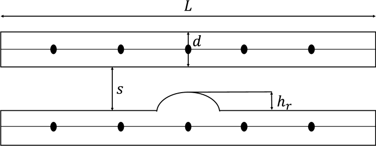
Figure 1: Sketch of the roughness modeling, $L$ and $d$ are length and diameter of the fiber, $h_{r}$ is the roughness height

Let us consider two fibers with diameter $d$ and length $L$ having surface roughness $h_{r}$=$\epsilon_{r}d$, where $\epsilon_{r}$ is the dimensionless roughness. The contact between the fibers takes place through the hemispherical asperity. The contact force exerted on the smooth surface is split into the force normal to the surfaces, $\mathbf{F}_{n}$ and the tangential force, $\mathbf{F}_{t}$. The normal contact force is modeled using a Hertz law

$$\mathbf{F}_{n}=-F_{0}\left(\frac{\delta}{L}\right)^{3/2}\mathbf{n},$$ (15)

where $\delta$ is the surface overlap defined as $\delta=h_{r}-s$, where s is the separation distance between the fibers and $F_{0}$ is the characteristic contact force scale in the suspension (Lobry et al., 2019; More & Ardekani, 2020c). The tangential force is modelled with the Coulomb’s friction law.

$$\mathbf{F}_{t}=\mu|\mathbf{F}_{n}|\frac{\mathbf{F}_{t}}{|\mathbf{F}_{t}|},$$ (16)

where $\mu$ is the friction coefficient that depends on material and tribological properties (Hasan et al., 2021a, b). It has been shown for spherical particle suspensions that a coefficient of friction decreasing with the normal load between the particles results in a shear thinning behavior (Lobry et al., 2019; More & Ardekani, 2020c). Hence, to model the shear thinning behavior exhibited by fiber suspensions (Bounoua et al., 2016), we also use a coefficient of friction decreasing with the normal load (Brizmer et al., 2007),

$$\mu=0.27\coth\left[{{{\left({\frac{{|\mathbf{F}_{n}^{(i,j)}|}}{{{F_{0}}}}}\right)}^{0.35}}}\right],$$ (17)

where $F_{0}$ is the characteristic force scale introduced in 15. The relative importance of contact to the hydrodynamics is estimated using dimensionless shear rate, $\dot{\Gamma}$ defined as

$$\dot{\Gamma}=\frac{{6\pi\eta{d^{2}}\dot{\gamma}}}{{{F_{0}}}},$$ (18)

where, $\dot{\gamma}$ is the imposed shear rate, and $\eta$ is the viscosity of the suspending fluid. To keep the $Re$ of the suspension constant, we vary $\dot{\Gamma}$ by varying the characteristic contact force scale $F_{0}$. It is well known that the rate-dependent rheology in suspensions is determined by the competition between various stress (force) scales (Guazzelli & Pouliquen, 2018; More & Ardekani, 2020d). Hence, by changing the value of $F_{0}$, we vary the relative contribution from the contact and hydrodynamic force in the suspension. Typically, $F_{0}$ depends on the fiber material properties like Young’s modulus, elastic modulus, Poisson’s ratio, etc. (Brizmer et al., 2007). However, this results in a very high value of $F_{0}$ restricting the time-step size to impractically small values ($<10^{-7}$) which makes the simulations computationally expensive. Hence, to resolve these numerical issues, we vary $F_{0}$ in orders of magnitudes of the hydrodynamic stress scale, i.e., $6{\pi}{\eta}{d^{2}}\dot{\gamma}$, as routinely done for spherical suspensions (Gallier et al., 2014; Mari et al., 2014; More & Ardekani, 2020b). This automatically allows us to vary $\dot{\Gamma}$, without changing the suspensions $Re$.

2.5 Boundary conditions and Domain size

We investigate suspensions of flexible fibers in a Couette flow, by varying the volume fraction, aspect ratio, flexibility, roughness, and inertia. The fibers are suspended in a channel with upper and lower walls moving in the x-direction with opposite velocities. No-slip and no penetration boundary condition is imposed on the wall and periodicity is assumed in the stream-wise, and span-wise directions. The fibers are initially distributed randomly. For this study we consider a domain of size $5L\times 5L\times 8L$ and $80\times 128\times 80$ grid points in the stream-wise, wall normal and span-wise direction, respectively as used in Banaei et al. (2020). Simulations are performed by placing the fibers randomly in the simulation cell. A sample configuration with reference frame is shown in figure 2. We repeated our simulation with 1.5, 2 ,2.5 and 3 times of the domain size and found a difference in the suspension viscosity lower than 2%. Moreover 17 Lagrangian points are chosen over the fibers which resolves the case with most flexible fibers. The required time-step to capture the fiber dynamics is $\Delta T=10^{-5}$. The suspension is simulated until a statistically steady viscosity is observed and only the average value is presented.

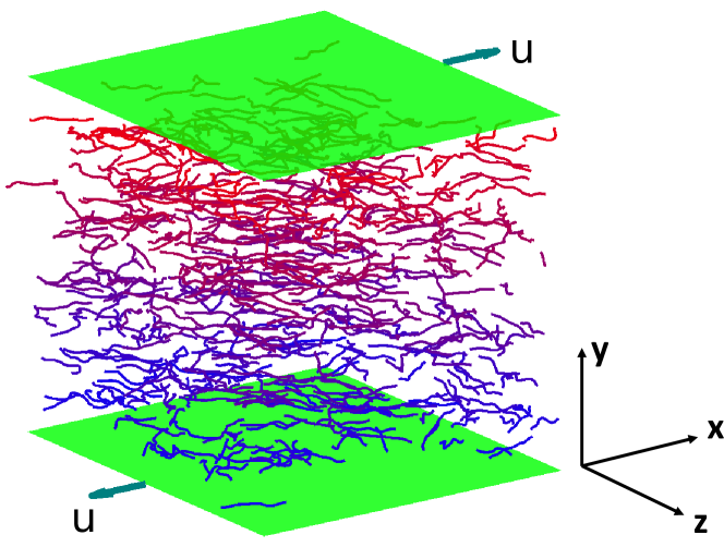
Figure 2: Example of configuration of fibers in a simulation cell

2.6 Stress and bulk rheology calculations

We compute the bulk stresses in the suspension to obtain the different rheological property. The dimensionless total stress is the summation of the fluid bulk stress and the stress generated by fluid-solid interactions:

$$\mathbf{\Sigma}_{ij}=\mathbf{\Sigma}{{}_{ij}^{0}}+\mathbf{\Sigma}{{}_{ij}^{f}},$$ (19)

with

$$\begin{array}[]{l}\mathbf{\Sigma}{{}_{xy}^{0}}=\frac{{{\mathop{\rm\textit{Re}}\nolimits}}}{V}\int\limits_{V-\sum{{V_{0}}}}{\left({-p{\delta_{ij}}+\frac{2}{{{\mathop{\rm\textit{Re}}\nolimits}}}{e_{ij}}}\right)}dV,\\ \mathbf{\Sigma}_{xy}^{f}=\frac{{{\mathop{\rm\textit{Re}}\nolimits}}}{V}\sum{\int\limits_{{V_{0}}}{{\sigma_{ij}}}dV},\end{array}$$ (20)

where $V$ is the total volume and $V_{0}$ is the volume of each fiber. Moreover, $\mathbf{\Sigma}_{ij}^{0}$ is the viscous fluid stress and $\mathbf{\Sigma}{{}_{ij}^{f}}$ is the stress generated by fluid-solid interactions due to the presence of fibers. The stress generated by contacts is included in the fluid-solid interaction stress. The fluid-solid interaction stress is decomposed into two parts:

$$\int\limits_{{V_{0}}}{{\sigma_{ij}}}dV=\int\limits_{{A_{0}}}{{\sigma_{ij}}}{x_{j}}{n_{k}}dA-\int\limits_{{V_{0}}}{\frac{{\partial{\sigma_{ik}}}}{{\partial{x_{k}}}}{x_{j}}}dV,$$ (21)

where $A_{0}$ represents the surface area of each fiber. The first term is called stresslet. The second term is identically zero for neutrally buoyant fibers when the relative acceleration of the fiber and fluid is zero. For slender bodies, the stresslet can be rewritten as:

$$\int\limits_{{A_{0}}}{{\sigma_{ij}}}{x_{j}}{n_{k}}dA=-r_{p}^{2}\int\limits_{L}{\mathbf{F_{i}}}{x_{j}}ds,$$ (22)

where $r_{p}$ is the aspect ratio of each fiber. Finally the total fiber stress is defined as:

$$\mathbf{\Sigma}{{}_{xy}^{f}}=-\frac{{{\mathop{\rm\textit{Re}}\nolimits}r_{p}^{2}}}{V}\mathbf{\Sigma}{\int\limits_{L}{\mathbf{F}_{i}}{x_{j}}ds}.$$ (23)

The details of the derivation are provided in Banaei et al. (2020). In this work, we present the relative viscosity and first normal stress difference to define the rheological behaviour of the suspension. The relative viscosity is defined as:

$$\eta_{r}=\frac{\eta_{eff}}{\eta},$$ (24)

where $\eta_{eff}$ is the effective viscosity of the suspension. The relative viscosity in terms of bulk stress is:

$$\eta_{r}=1+\mathbf{\Sigma}{{}_{xy}^{f}},$$ (25)

where $\mathbf{\Sigma}{{}_{xy}^{f}}$is time and space average shear stress arising from the presence of the fiber. $\mathbf{\Sigma}{{}_{xy}^{f}}$ is non-dimentionalised by viscosity $\eta$ and shear rate $\dot{\gamma}$. The first normal stress difference $N_{1}$ is defined as:

$$N_{1}=\mathbf{\Sigma}{{}_{xx}}-\mathbf{\Sigma}{{}_{yy}}.$$ (26)

2.7 Simulation parameters

The aim of this study is to investigate the effect of flexibility, aspect ratio, and roughness on the suspension rheology and jamming fraction in the presence of friction. The different quantities are made dimensionless by the viscous scale for the current study. The fiber dimensionless bending stiffness is defined as

$$\widetilde{B}=\frac{\pi}{4}r_{p}^{2}{\mathop{\rm\textit{Re}}\nolimits}B,$$ (27)

with $B$ defined in equation (5). The volume fraction of the suspension is defined as

$$\phi=\frac{{n\pi r_{p}^{2}}}{{4V}},$$ (28)

where $r_{p}$ is the aspect ratio of the fiber. We simulate a shear flow by varying the Reynolds number in the range  $1\leq Re\leq 10$, the fiber bending rigidity in the range $0.005\leq\tilde{B}\leq 0.2$, the roughness height in the range $.005\leq\epsilon_{r}\leq 0.1$, the dimensionless shear rate in the range $1\leq\dot{\Gamma}\leq 1000$, and the aspect ratio in the range $10\leq AR\leq 16$. Note that as $\tilde{B}$ increases, fiber becomes more rigid. The volume fraction depends on the aspect ratio of the fiber with a maximum of 0.5 for the less slender fibers. All the cases considered in the present work are reported in table 1.

Re	$\epsilon_{r}$	$\dot{\Gamma}$	$\phi$	$AR$	$\tilde{B}$
$1,5,10$	00 $0.005-0.1$0	00$1-1000$0	00 $0.05-0.50$0	00$10-16$0	00$0.005-0.2$

Table 1: Summary of the numerical simulations performed in this study

3 Results

3.1 Shear rate dependent rheology

The objective of the study is to find the shear rate dependent behaviour when varying the suspension volume fraction, flexibility, and roughness of the fibers.

\begin{overpic}[width=433.62pt]{Shear_rate/Volume_fraction.eps} \put(54.0,50.0){$\tiny{\color[rgb]{0,0,1}{\boldsymbol{\eta_{r}=26.47\dot{\Gamma}^{-0.381}}}}$} \put(20.0,31.0){$\tiny{\color[rgb]{0,1,0}{\boldsymbol{\eta_{r}=7.58\dot{\Gamma}^{-0.232}}}}$} \put(18.0,18.0){$\tiny{\color[rgb]{1,0,0}{\boldsymbol{\eta_{r}=2.86\dot{\Gamma}^{-0.156}}}}$} \end{overpic}

(a)

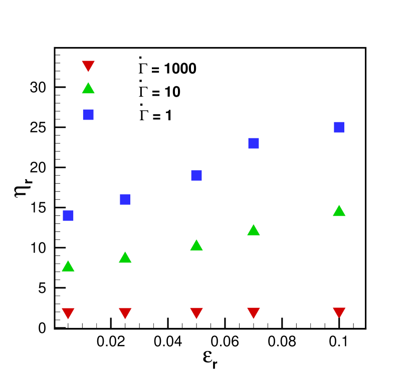
(b)

Figure 3: Relative viscosity of fiber suspensions versus (a) the applied shear rate at different volume fractions. The dashed line represents the power law fit. The power law indices for different volume volume fractions are : for $\phi=5\%,$ $k=2.86$ and $n=0.156$; for $\phi=10\%,$ $k=7.58$ and $n=0.232$; and for $\phi=15\%,$ $k=26.47$ and $n=0.381$. The roughness height was fixed to $\epsilon_{r}$ = 0.05 and AR = 16 for all cases. (b) the roughness height at different applied shear rates. The suspension volume fraction is fixed to $\phi=0.10$ and bending rigidity to $\tilde{B}=0.02$.

Figure 3 displays the computed relative viscosity as a function of reduced shear rate, $\dot{\Gamma}$ for different volume fractions and roughness heights. We observe from figure 3(a) that the viscosity decreases as the reduced shear rate increases due to the reduction of the friction coefficient similarly to the findings of More & Ardekani (2020c). The shear thinning behavior matches the experimental results reported by Bounoua et al. (2016). We provide a power law fit to show how the power law index changes with the volume fraction as follows :

$$\eta(\dot{\Gamma})=k\dot{\Gamma}^{-n}.$$ (29)

The viscosity shows two plateaus, one at high reduced shear rates and one at low reduced shear rates. The plateau at a high shear rate is due to the saturation of the friction coefficient at high normal loads. As the volume fraction increases, the contact between the fibers increases, which causes the higher relative viscosity at higher volume fractions for a particular reduced shear rate.

Figure 3(b) shows the effect of increasing roughness from 1% to 10% at different reduced shear rates for a fixed volume fraction, $\phi=10\%$. We see that the relative viscosity increases with roughness and this increase in viscosity is higher at lower shear rates. For $\dot{\Gamma}=1000$, the relative viscosity is almost independent on the roughness. However, as $\dot{\Gamma}$ is reduced to 1, the increase in viscosity is higher at roughness height 0.005 compared to roughness height 0.1. With the increase in the shear rate, the shear stress also increases and correspondingly there is an increase in the normal forces between fibers, and a reduction of the coefficient of friction. As a result we observe a reduction in the relative viscosity much higher at lower shear rates than for higher shear rates with roughness.

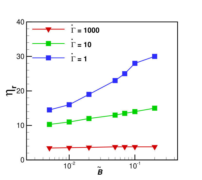
(a)

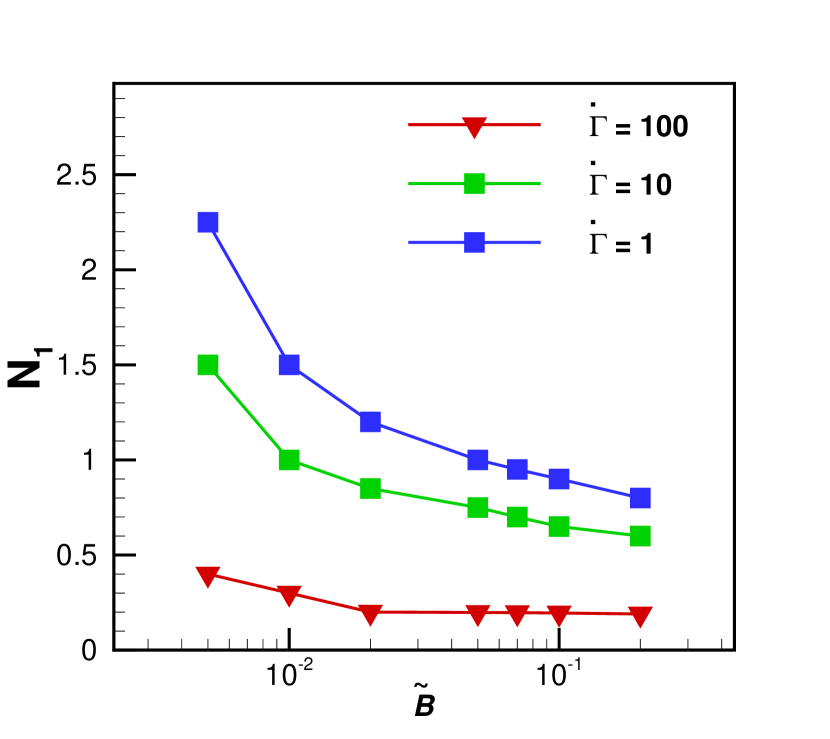
(b)

Figure 4: (a) Relative viscosity vs bending rigidity and (b) First normal stress as a function bending rigidity for different shear rates. All simulations were performed with $\phi=10\%$, $\epsilon_{r}=0.05$, $\tilde{B}=0.02$ and $AR=16$

.

We present the relative viscosity and first normal stress versus the fiber stiffness and for different shear rates in figure 4(b). Figure 4(a) shows the increase in viscosity with bending rigidity which is in an agreement with experiments (Goto et al., 1986; Sepehr et al., 2004). It can be explained by the fact that flexible fibers tend to align with the flow direction more easily compared to rigid fibers as also observed for deformable spheres (Rosti & Brandt, 2018). Our results contradict the results of Wu & Aidun (2010b) who obtained a large viscosity for more flexible fibers. These authors considered rigid particles interconnected by a chain that can bend and twist at their joints; leading to higher stresses than for continuous fibers which can only bend. This higher stress leads to higher viscosity compared to us as we are considering a continuous fibers which can only bend. We also observe that the effect of fiber flexibility in concentrated suspensions is more significant at lower shear rates than at higher shear rates.

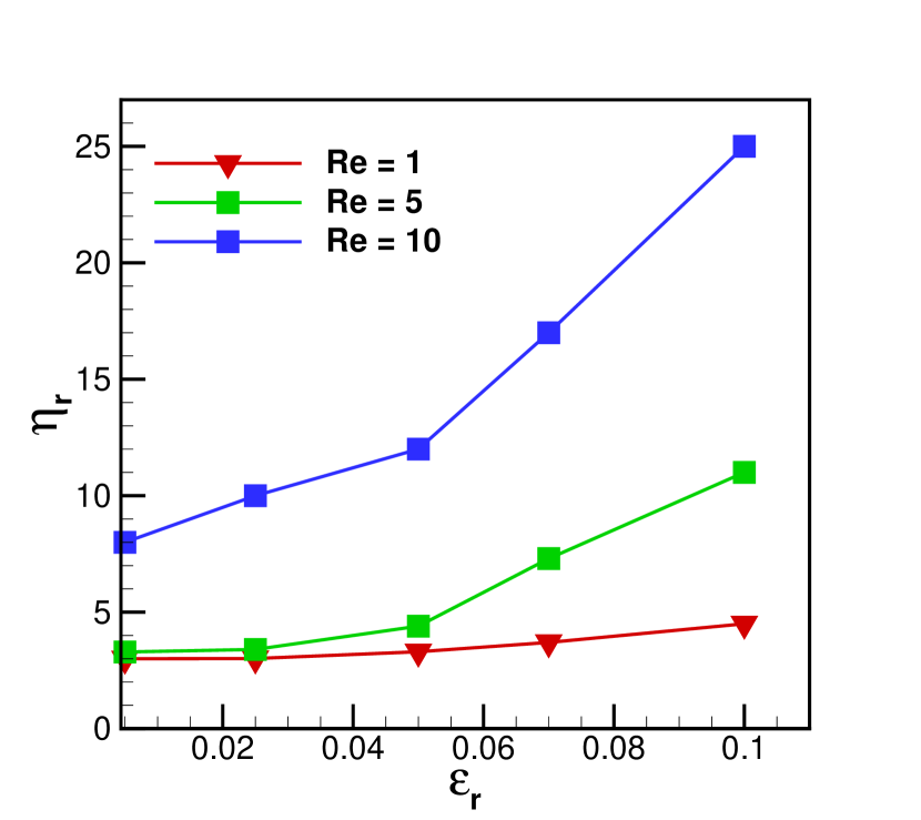
(a)

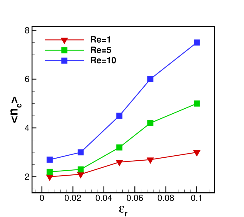
(b)

Figure 5: (a) Relative viscosity of fiber suspensions and (b) Average number of fiber contacts as a function of roughness height. All the cases consider a fixed shear rate, $\dot{\Gamma}=1000$, $\tilde{B}=0.02$, and $AR=16$

.

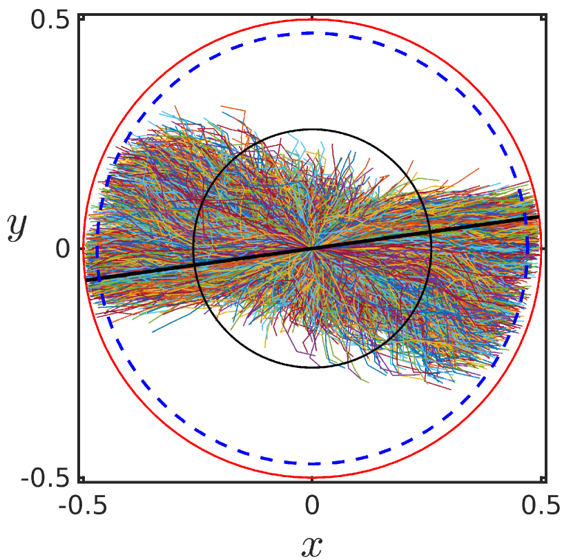
(a)

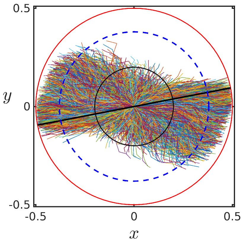
(b)

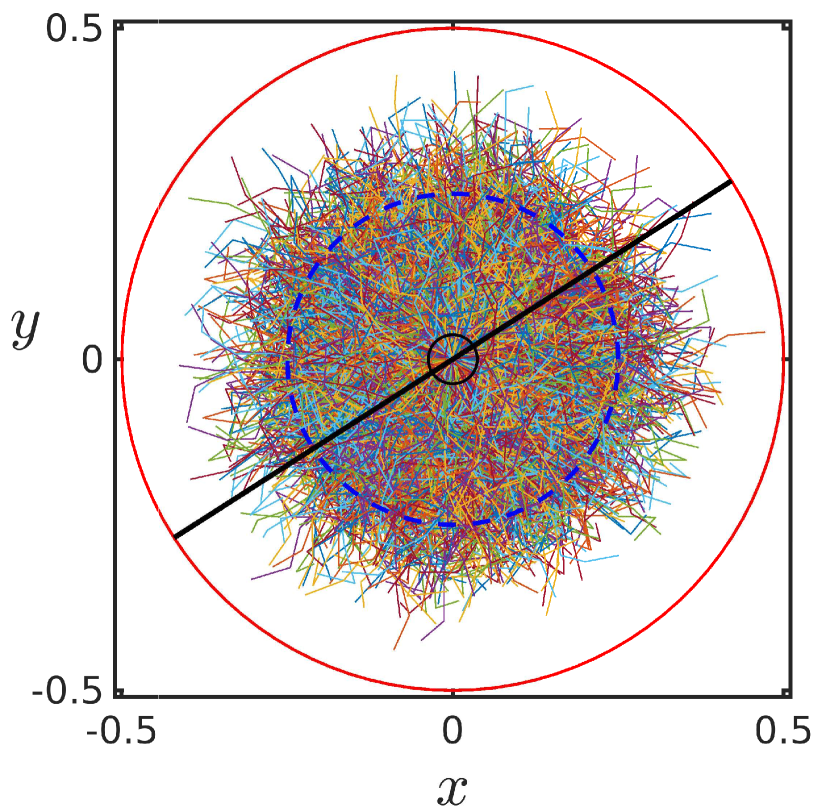
(c)

Figure 6: Co-located filaments projected on the shear plane for (a) $\epsilon_{r}=.005,Re=1$, (b) $\epsilon_{r}=0.10,Re=1$ and (c) $\epsilon_{r}=0.005,Re=5$. The solid red line represents the circles with diameter equal to the fiber length, the blue dashed line is the circle with diameter equal to the mean end to end distance and the black circles have diameter equal to the minimum end to end distance between fibers. The solid black line shows the average orientation of the fibers with respect to the wall. All simulations were performed with $\dot{\Gamma}=1000$, $\phi=10\%$, $\tilde{B}=0.02$ and $AR=16$.

.

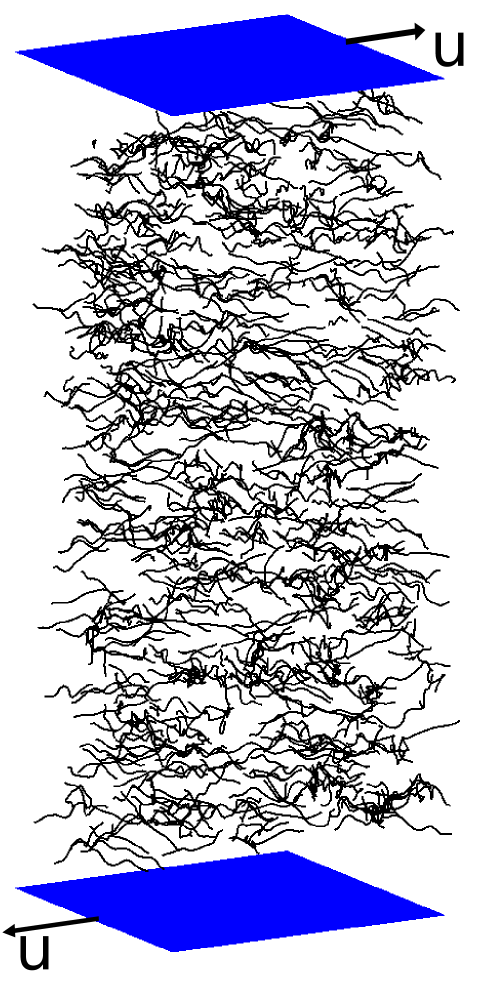
(a)

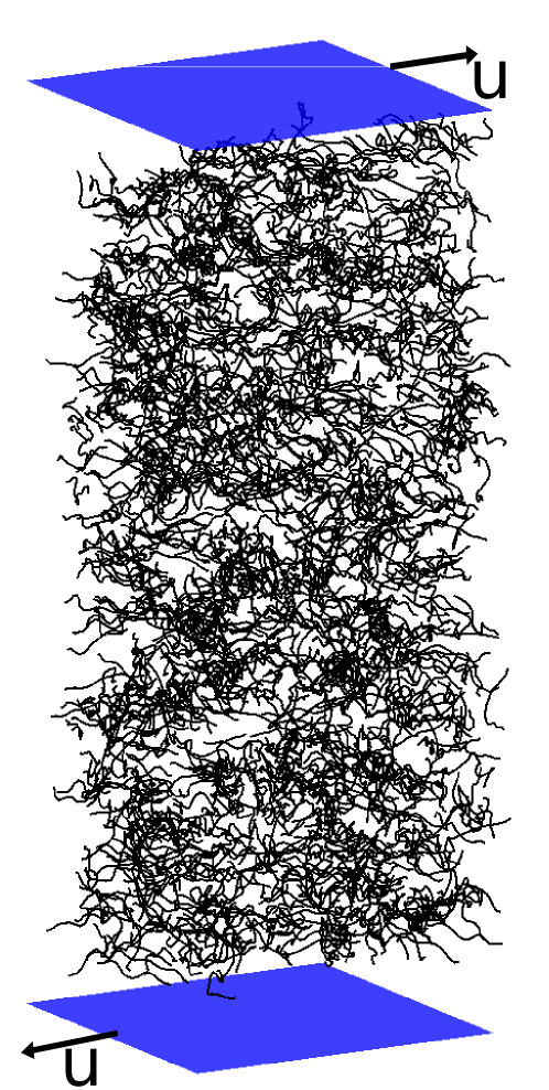
(b)

Figure 7: Simulation snapshots at a thin slice in the middle of the simulation cell after shearing to a strain of $\dot{\Gamma}=1000$ with parameters $Re=5$, $\tilde{B}=0.02$, and (a) roughness $\epsilon_{r}=.005$ (b) roughness $\epsilon_{r}=.10$

.

In fiber suspensions, due to the presence of hydrodynamics and solid-body interactions, normal stress differences inevitably arise (Keshtkar et al., 2009). The second normal stress is much smaller than the first normal stress and can be neglected (Petrich et al., 2000; Sepehr et al., 2004). We report the effect of fiber flexibility on the first normal stress difference in figure 4(b) . The first normal stress is positive as expected. Moreover, the first normal stress difference decreases as the fibers become more rigid; in agreement with the observation in Keshtkar et al. (2009). The increase in the first normal stress with flexibility is more pronounced at a lower shear rate when friction forces are more relevant.

3.2 Effect of Inertia

To better understand the effect of inertia on the suspension behavior, we run simulations for $Re=1,5$, and $10$ by varying the volume fraction, $\phi=4\%$ to $16\%$, roughness height, $\epsilon_{r}=1\%$ to $10\%$ and bending rigidity, $\tilde{B}=0.005$ to $0.2.$

Figure 5(a) displays the effect of roughness height on the relative viscosity for $Re=1,5,$ and $10$ with a fixed volume fraction, $\phi=10\%$, aspect ratio, $AR$ 16 and shear rate, $\dot{\Gamma}=1.0$. The viscosity increases with roughness, an effect more evident at a higher Reynolds number. In figure 5(b), we present the average number of fiber contacts, $<n_{c}>$, as a function of roughness height for different Reynolds numbers. We observe an increase in $<n_{c}>$ with roughness. This leads to a higher viscosity for rough fibers that is more evident at high inertia.

In order to visualize the fiber deformation with roughness and inertia, we consider them co located with their center positioned at their origin of the axis. In figure 6(c), we show the projection of the fiber configuration for smooth $(\epsilon_{r}=.005)$ and rough fibers $(\epsilon_{r}=0.10$ with low inertia $(Re=1.0)$ and high inertia $(Re=5)$. The solid red line represents the circle having diameter equal to the length of the fibers, whereas the dashed blue lines denote circles having diameters equal to the mean end to end distance. The solid black line represents the average orientation of the fibers with respect to the flow direction. From figure 6(a) and 6(b) we observe that increasing roughness causes larger deformation of the fibers and also decreases the alignment of the fibers with the flow direction. Smooth surface leads to a reduced chance of fiber interlocking and consequently reduced fibre contacts. So they tend to align in the flow direction with a small number of contact force chains scattered throughout the shear cell. Hence, smoothing the fiber surface, as well as reducing the friction coefficient, decreases the contacts between fibers which leads to lower viscosity of the suspension. For $\epsilon_{r}=0.10$ and $Re=5$ (high inertia and rough fibers), the majority of the fiber exhibit significant bending and the mean and minimum end to end distance is smaller than for the case at lower inertia in figure 6(b). Moreover, the fibers tend to be at larger angles with the flow direction at high Reynolds number which causes increase in flow resistance and enhances the viscosity of the suspension. In figure 7(b), we present snapshots of a thin slice in the middle of the simulation cell for suspension of smooth and rough fibers for a fixed Reynolds number, $Re=5$. We observe that for higher roughness height, ${\epsilon_{r}=.10}$, fibers tend to agglomerate more compared to smooth fibers, ${\epsilon_{r}=.005}$.

To better understand the rheology, we investigate the different contributions to the total shear shear stress in the suspension. Figure 8(a) reports the relative contribution of viscous and fluid-solid interaction stresses to the total shear stress for the case of low inertia, $Re$=1, and different values of roughness, $\epsilon_{r}$. The Reynolds stress is negligible for the values of Re investigated (Banaei et al., 2020) and is not reported in the figure. Figure 8(a) reveals that the relative contribution to the total stress from the suspended fibers increases as the fiber roughness is increased. Besides, figure 8(b) shows the effect of the Reynolds number on the stress budget for a fixed roughness height, $\epsilon_{r}=0.05$. The contribution from fluid-solid interaction increases with the Reynolds number. Thus, the large increase in the viscosity, reported in figure 5(b), is due to the increased fluid-solid interaction forces whereas the viscous contribution is almost unchanged in the suspension at high Reynolds numbers.

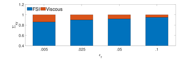
(a)

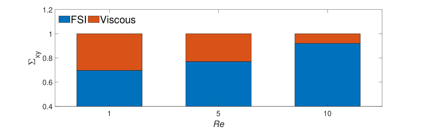
(b)

Figure 8: Stress Budget. Relative contribution to the total stress from fluid-solid interaction and viscous effect vs (a) the roughness at a fixed Reynolds number, $Re=1$ (b) for different Reynolds number at a fixed roughness, $\epsilon_{r}=0.05$. The contributions to the shear stress from fluid-solid interaction and viscous effect are normalized by the total shear stress for each case.

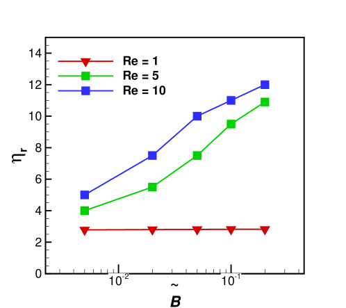
Figure 9: Relative viscosity of fiber suspension vs Fiber rigidity. All the cases are performed with a fixed shear rate, $\dot{\Gamma}=1000$, Aspect ratio, $AR=16$, and roughness, $\epsilon_{r}=0.05$

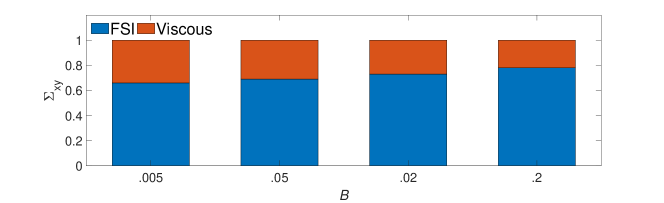
(a)

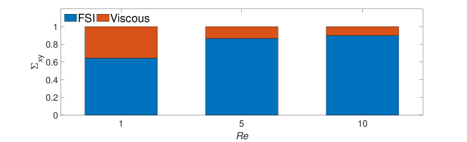
(b)

Figure 10: Stress Budget. Relative contribution to the total stress from fluid-solid interaction and viscous vs (a) the bending rigidity at a fixed Reynolds number, $Re=1$ (b) for different Reynolds’s number at fixed bending rigidity, $\tilde{B}=0.2$. The contributions to the shear stress from fluid-solid interaction and viscous effect are normalized by the total shear stress for each case.

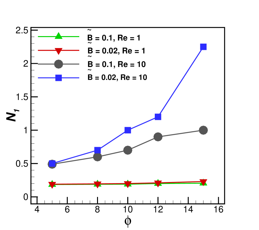
(a)

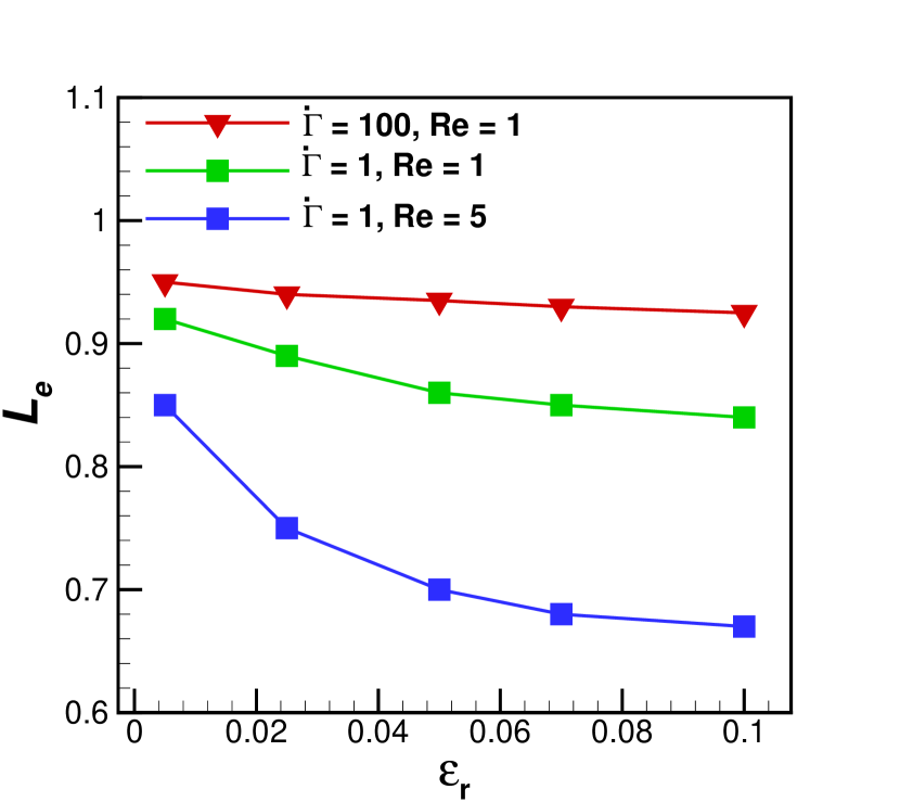
(b)

Figure 11: (a) First normal stress difference as a function of the fiber volume fraction for different Reynolds numbers and flexibility, and (b) Mean end to end distance of fiber vs roughness height as a function of Shear rate and Reynolds number for bending rigidity, $\tilde{B}=0.2$. All simulations are reported for fixed aspect ratio, $AR=16$ and roughness, $\epsilon_{r}=0.05$

.

Figure 9 shows the effect of fiber rigidity, $\tilde{B}$ on the suspension viscosity, $\eta_{r}$ for three different values of the Reynolds numbers. We observe that the relative viscosity increases with the fiber rigidity, especially at a high Reynolds number. In concentrated suspensions, for a fixed volume fraction, larger fiber stiffness leads to an increase in the contact forces. Flexible frictional fibers tend to roll into round agglomerates under shear, while stiffer fibers are more resistant to bending, remain straight and tend to align with the flow direction. As a result, high resistance to the flow is observed for stiffer fiber suspensions, which in turn increases the viscosity.

For low Reynolds numbers, e.g. $Re=1$, the relative viscosity, $\eta_{r}$ is almost constant with rigidity, $\tilde{B}=0.2$. Relative viscosity, $\eta_{r}$ increases with the Reynolds number the most for the most stiff case. Thus, inertial effects are more evident for rigid fibers than flexible fibers. In figure 10(a), we report the contribution of the viscous and FSI contributions to the total stress to the total stress of the suspension for different bending rigidity values and $Re=1$. For a low Reynolds number, as the fiber becomes more and more flexible, the contribution from the fluid-solid interaction is decreases. Moreover, the fiber flexibility affects the suspension and the fiber contribution increases at high Reynolds numbers as reported in figure 10(b). The increase of the stress component due to the fluid-solid interaction can be related to the increase in the drag force experienced by the fibers at finite inertia, similarly, to what previously observed for cylinders and spheres (Fornberg, 1980; Banaei et al., 2020).

In addition to the relative viscosity, we document the relevance of inertial effect on the first normal stress difference of the suspension. Figure 11(a) reports the first normal stress difference as a function of volume fraction, Reynolds number and fiber flexibility. Our simulations report a positive first normal stress difference for all cases, which agrees with the experiments by (Keshtkar et al., 2009; Snook et al., 2014). The first normal stress difference increases with the volume fraction due to the increase in the interaction between fibers. However, the increase in first normal stress difference with the volume fraction is more visible at a high Reynolds number, $Re$=10. The first normal stress difference is larger for flexible fibers compared to rigid fibers, which agrees with the experiment of nylon fibers reported in (Keshtkar et al., 2009). At low Reynolds number, $Re=1$, the first normal stress difference is almost the same for flexible and rigid fibers. At $Re=10$, the flexible fiber suspensions exhibits a higher first normal stress difference, already noticeable at 8% volume fraction. To observe the fiber deformation with roughness and Reynolds numbers at different shear rates, we plot the mean end to end distance for the flexible fibers, $B=.02$ in figure 11(b). The larger deformation is observed at a high surface roughness which becomes more pronounced at a high Reynolds number. At a low Reynolds number, $Re=1$, the deformation is observed only at a low shear rate and higher roughness. The larger deformation observed at the high Reynolds number and high roughness is attributed to increased fiber-fiber interactions at higher roughness values.

3.3 Jamming

At a high solid concentration, a solid-like phase is formed which strongly resists the flow defined as jamming. In this section, we find the jamming volume fractions for different aspect ratios and roughness values.

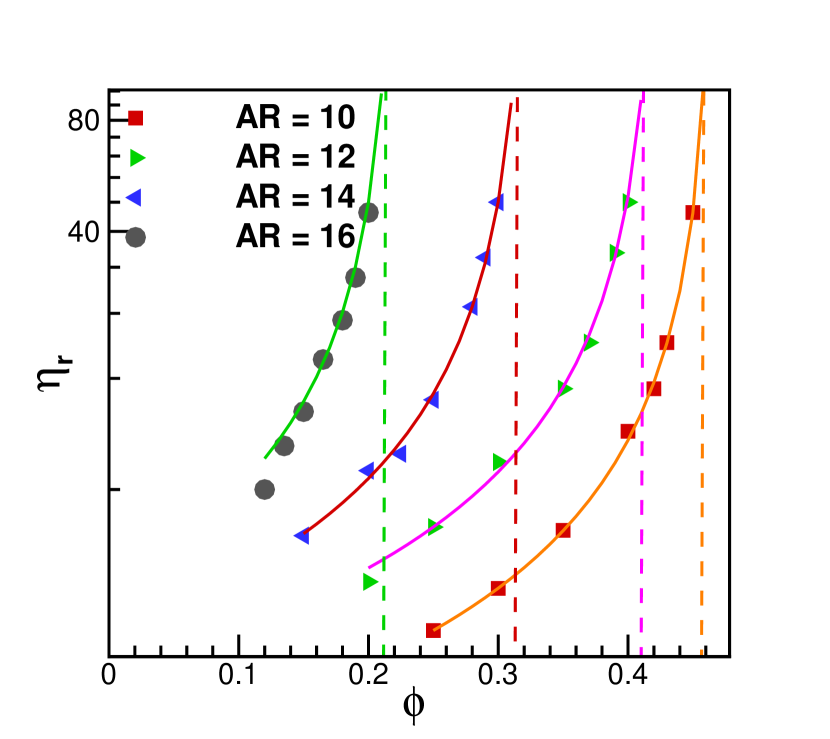
(a)

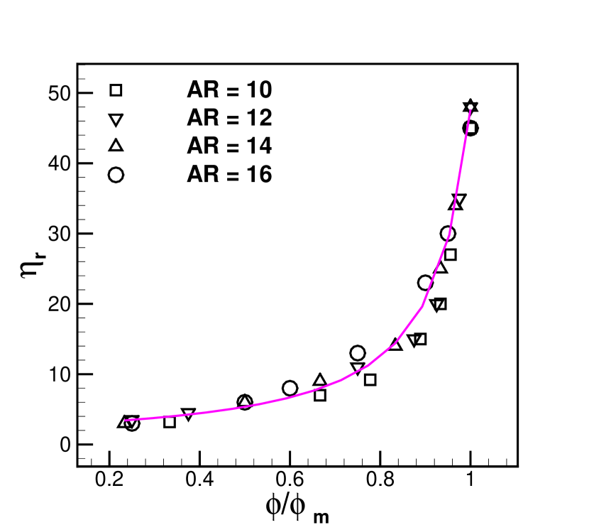
(b)

Figure 12: (a) relative viscosity vs volume fraction for different aspect ratios (b) Rescaled rheological data for different aspect ratios.

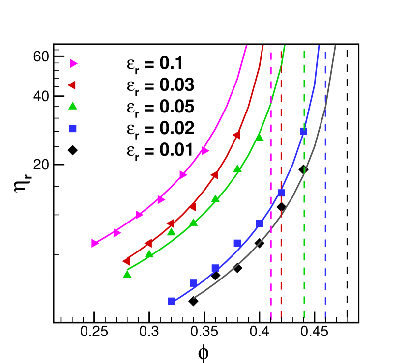
(a)

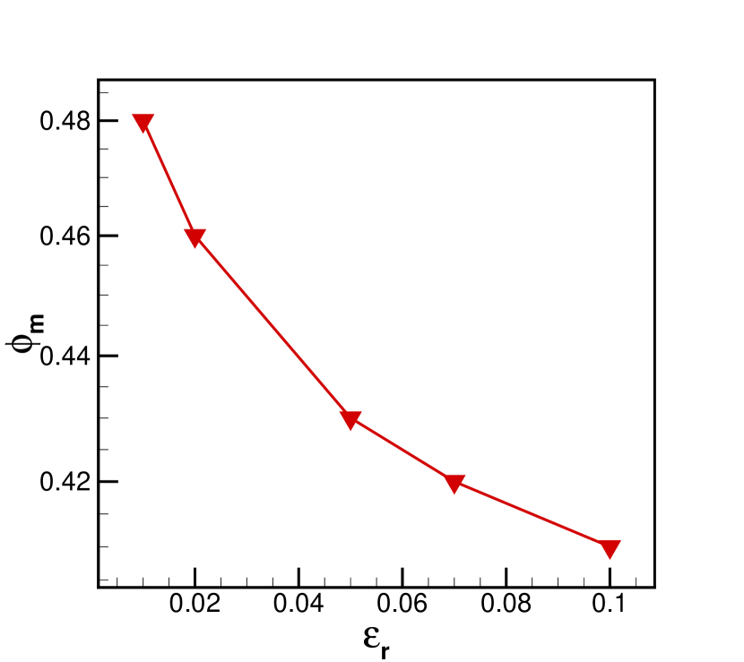
(b)

Figure 13: (a) relative viscosity vs volume fraction for different surface roughness values. The jamming volume fraction tends to decrease with increase in roughness because of the increase in friction coefficient with roughness (b) maximum volume fraction vs roughness height. All simulations were performed for a fixed Reynolds number, $Re=1$ and bending rigidity, $\tilde{B}=.02$

We present the results obtained by varying the aspect ratio as $10,12,14$, and 16 for a fixed roughness height $\epsilon_{r}=0.1$, Reynolds number, Re=1 and reduced shear rate, $\dot{\Gamma}=1.0$. We observe in figure 12(a) that the viscosity increases with the volume fraction and diverges at a maximum volume fraction that depends on the aspect ratio. The maximum volume fraction above which the suspension is jammed and no flow is possible is called the jamming volume fraction, $\phi_{m}$. To find the jamming volume for a particular aspect ratio, we fit the data pertaining the viscosity as function of volume fraction, $\phi$ with the following modified Maron-Pierce law:

$$n_{r}=\alpha(1-\phi/\phi_{m})^{-\beta},$$ (30)

with parameters $\alpha$, $\phi_{m}$, $\beta$, depending on the aspect ratio and roughness of the fibers.

$AR$	$\alpha$	$\phi_{m}$
$10$	0 $1.54$0	0$0.47$0
$12$	0$2.58$0	0$0.42$0
$14$	0$3.24\hphantom{0}$	0$0.32$0
$16$	0$4.42$0	0$0.22$0

Table 2: Fitting parameters for different aspect ratios for a fixed roughness height, $\epsilon_{r}=0.1$

The fitting parameters are presented in table 2, and the solid lines in figure 12(a) represent the fitting curve given in equation (30). We find that the relative viscosity diverges near the jamming transition with a scaling of $(\phi_{m}-\phi)^{-1}$ in contrast with the behavior $(\phi_{m}-\phi)^{-2}$ observed for suspension of spheres (Boyer et al., 2011; Cates & Wyart, 2014). Tapia et al. (2017) reported the jamming transition with a scaling of $(\phi_{m}-\phi)^{-0.90}$ for suspension of rigid fibers. Figure 12(b) shows the data after re-scaling the volume fraction of figure 12(a) by $\phi_{m}$ which leads to a collapse of the data indicating that the aspect ratio determines the maximum volume fraction once the fiber flexibility and roughness are fixed. The effect of varying aspect ratio is clear from both figures. For the minimum aspect ratio, i.e., $AR$ = 10, we find $\phi_{m}=0.47$. Increasing the aspect ratio to 16, the maximum volume fraction reduces to 0.2. In concentrated suspension, elongated fibers have a larger probability of inter-fiber contacts. As a result, there is an increase in the contact force which in turn increases the shear stress. Thus, the viscosity increases with the aspect ratio for a fixed volume fraction and this results in a reduction of the jamming fraction with aspect ratio.

Indeed, the concentrated regime is defined in fibers suspension as a function of aspect ratio. If $\phi>\frac{1}{r_{p}}$, the fiber-fiber interaction is dominant in determining the suspension behavior. Thus, for aspect ratio 16, the concentrated regime occurs when $\phi>.053$. But for a lower aspect ratio, fiber-fiber contact starts to dominate at a higher volume fraction. For example, for aspect ratio 12, the concentrated regime is reached when $\phi>0.10$. As a result, a much higher volume fraction can be achieved in the suspension until the suspension jams. As the aspect ratio increases, the effective fiber volume also increases, resulting in a denser contact network with higher contact stresses. Eventually, this leads to the increase in viscosity and reduction of jamming volume fraction.

$\epsilon_{r}$	$\alpha$	$\phi_{m}$
$0.01$	0 $1.51$0	0$0.48$0
$0.02$	0 $2.10$0	0$0.46$0
$0.03$	0 $2.50$0	0$0.43$0
$0.05$	0 $2.57$0	0$0.42$0
$0.10$	0 $3.50$0	0$0.40$0

Table 3: Fitting parameters for different roughness values for a fixed aspect ratio, $AR=10$

Next, we would like to know the effect of varying roughness on the volume fraction at jamming. We therefore vary the roughness between 0.01 to 0.1 for a fixed aspect ratio, $AR=12$. As before, we find the jamming fraction, $\phi_{m}$ by fitting the data with equation (30), where the coefficients $\alpha$, $\phi_{m}$, and $\beta$ depend on the roughness height, $\epsilon_{r}$. The fitting parameters are presented in table 3, whereas the solid line in figure 13(a) represents the fitting curve given in equation (30). We find the relative viscosity diverges near the jamming transition with a scaling of $(\phi_{m}-\phi)^{-1}$. Moreover, we observe the jamming fraction decreases with increasing the roughness. Due to the denser contact network with increasing roughness, the viscosity of the suspension increases for a particular volume fraction. For the smoothest case, $\epsilon_{r}=0.01$, we find $\phi_{m}=0.47$, whereas for the roughest case $\epsilon_{r}=0.1$, $\phi_{m}$ is as low as 0.41. The decrease in $\phi_{m}$ is expected due to an increase in the effective volume with roughness that results in a denser contact network. It eventually leads to an increase in the viscosity and a decrease in the jamming volume.

4 Conclusion

We have investigated, by means of numerical simulations, the rheological behaviour of concentrated fiber suspensions for a range of Reynolds numbers, aspect ratios, bending rigidity, and roughness. The flows we have considered in our simulations have inertial effects but the flow is still viscous dominated and Reynolds number is small. We present the macroscopic properties of suspension and discuss the stress budget and fiber deformation to disentangle the mechanisms at work. We considered fibers as one dimensional in-extensible slender bodies obeying Euler-Bernoulli beam equation, suspended in an incompressible Newtonian fluid. The coupling between fluid and solid motion is done using an immersed boundary method. It is assumed that fibers come into contact through a few asperities and the value of the friction coefficient varies with the normal load. In this model, we include the contact law presented by Brizmer et al. (2007), where the coefficient of friction decreases at low normal loads followed by a plateau at high normal loads. This causes a decrease in viscosity with shear rate. By implementing this contact model, we can capture the shear thinning rheological behaviour in fiber suspensions as observed in experiments (Bounoua et al., 2016).

In this work, we focus on the effect of friction and its role on the rheological properties, especially the relative viscosity and first normal stress difference. We show that the friction has substantial impact of the rheology of fibers suspension. First, we present the shear rate dependent macroscopic properties when varying roughness, volume fraction, and fiber flexibility. The viscosity is found to increase with the the fiber volume fraction, the roughness and the fiber rigidity. These effects are more pronounced at lower shear rates. As the roughness increases, the contact force increases, which in turn increases the average number of contacts in the suspension and consequently fluid-solid interactions. More rigid fibers bend less and are less aligned with the flow. They create less ordered structures which increases the flow resistance. The increase in viscosity with roughness and fiber rigidity is more pronounced at high Reynolds numbers. From the stress budget, we observe an increase in the stress contribution from the fluid-solid interaction with roughness and fiber rigidity. In agreement with the experiments by Keshtkar et al. (2009), we find the normal stress difference to be positive. It increases with the volume fraction, especially at higher Reynolds numbers. Flexible fiber suspensions exhibit a higher first normal stress, which is also in agreement with the experiments by Keshtkar et al. (2009).

Lastly, we explored the divergence of viscosity at the maximum packing fraction and proposed a relation to model the divergence. The aspect ratio and roughness of fibers impact the maximum volume fraction. A modified Maron-pierce law has been proposed to find the jamming volume fraction for different aspect ratios and asperity sizes. Rescaling the volume fraction by packing value, $\phi_{m}$, collapses the data into a single curve denoting that the aspect ratio principally effect the maximum volume fraction if the roughness is fixed. The increase in the viscosity with aspect ratio is attributed to the increase in the number of contacts and the contact force, which in turn increases the suspension shear stress. We also find the jamming fraction for different roughness values of the fibers. As the roughness of the fiber increased, the suspension jams at a lower volume fraction. With the increase of the roughness, the effective volume fraction decreases resulting in a denser contact network. As a result the average coefficient of friction increases, which in turn reduces the jamming fraction. We find the viscosity to diverge as $(\phi_{m}-\phi)^{-1}$, in contrast with spherical suspensions, where viscosity diverges as $(\phi_{m}-\phi)^{-2}$.

Our results demonstrate the importance of modeling friction and contact force to capture the global behavior of the suspension. One of the fundamental mechanisms that governs the rheological behavior of sheared fibers suspension is the increase in the friction coefficient with roughness. Since it is challenging to modify the coefficient of friction, we can modify other properties of fibers that influences friction such as roughness to modify suspension properties according to the need to different applications. Additionally, our results indicate that to have higher solid concentrations that are desirable in industrial applications, we should breakdown the fibers into smaller sizes, pretreat them to be more flexible, and use processes to make the surface smoother. To get a more quantitative prediction of the physical mechanisms of shear thinning behavior, the next step would be to determine the friction law between fibers form atomic force microscopy measurement.

ACKNOWLEDGEMENT

AMA would like to acknowledge financial support from the Department of Energy via grants EE0008256 and EE0008910. This work used the Extreme Science and Engineering Discovery Environment (XSEDE) (Towns et al., 2014), which is supported by the National Science Foundation grant number ACI-1548562 through allocations TG-CTSI190041. L.B. acknowledges financial support from the Swedish Research Council (VR) and the INTERFACE research environment (Grant No. VR 2016-06119)

Declaration of Interests. The authors report no conflict of interest.

References

- Alizad Banaei et al. (2017) Alizad Banaei, A. , Loiseau, J.-C. , Lashgari, I. & Brandt, L. 2017 Numerical simulations of elastic capsules with nucleus in shear flow. European Journal of Computational Mechanics 26 (1-2), 131–153.
- Banaei et al. (2020) Banaei, A. A. , Rosti, M. E. & Brandt, L. 2020 Numerical study of filament suspensions at finite inertia. Journal of Fluid Mechanics 882.
- Batchelor (1971) Batchelor, G. 1971 The stress generated in a non-dilute suspension of elongated particles by pure straining motion. Journal of Fluid Mechanics 46 (4), 813–829.
- Bibbó (1987) Bibbó, M. A. 1987 Rheology of semiconcentrated fiber suspensions. PhD thesis, Massachusetts Institute of Technology.
- Blakeney (1966) Blakeney, W. R. 1966 The viscosity of suspensions of straight, rigid rods. Journal of Colloid and Interface Science 22 (4), 324–330.
- Bounoua et al. (2016) Bounoua, S. , Lemaire, E. , Férec, J. , Ausias, G. & Kuzhir, P. 2016 Shear-thinning in concentrated rigid fiber suspensions: Aggregation induced by adhesive interactions. Journal of Rheology 60 (6), 1279–1300.
- Boyer et al. (2011) Boyer, F. , Guazzelli, É. & Pouliquen, O. 2011 Unifying suspension and granular rheology. Physical Review Letters 107 (18), 188301.
- Brizmer et al. (2007) Brizmer, V. , Kligerman, Y. & Etsion, I. 2007 Elastic–plastic spherical contact under combined normal and tangential loading in full stick. Tribology Letters 25 (1), 61–70.
- Butler & Snook (2018) Butler, J. E. & Snook, B. 2018 Microstructural dynamics and rheology of suspensions of rigid fibers. Annual Review of Fluid Mechanics 50, 299–318.
- Cates & Wyart (2014) Cates, M. E. & Wyart, M. 2014 Granulation and bistability in non-brownian suspensions. Rheologica Acta 53 (10-11), 755–764.
- Djalili-Moghaddam & Toll (2006) Djalili-Moghaddam, M. & Toll, S. 2006 Fibre suspension rheology: effect of concentration, aspect ratio and fibre size. Rheologica acta 45 (3), 315–320.
- Fornberg (1980) Fornberg, B. 1980 A numerical study of steady viscous flow past a circular cylinder. Journal of Fluid Mechanics 98 (4), 819–855.
- Gallier et al. (2014) Gallier, S. , Lemaire, E. , Peters, F. & Lobry, L. 2014 Rheology of sheared suspensions of rough frictional particles. Journal of Fluid Mechanics 757, 514–549.
- Goto et al. (1986) Goto, S. , Nagazono, H. & Kato, H. 1986 The flow behavior of fiber suspensions in newtonian fluids and polymer solutions. Rheologica acta 25 (2), 119–129.
- Guazzelli & Pouliquen (2018) Guazzelli, É. & Pouliquen, O. 2018 Rheology of dense granular suspensions. Journal of Fluid Mechanics 852.
- Guo et al. (2020) Guo, Y. , Li, Y. , Liu, Q. , Jin, H. , Xu, D. , Wassgren, C. & Curtis, J. S. 2020 An investigation on triaxial compression of flexible fiber packings. AIChE Journal 66 (6), e16946.
- Guo et al. (2015) Guo, Y. , Wassgren, C. , Hancock, B. , Ketterhagen, W. & Curtis, J. 2015 Computational study of granular shear flows of dry flexible fibres using the discrete element method. Journal of Fluid Mechanics 775, 24–52.
- Hasan et al. (2021a) Hasan, M. S. , Kordijazi, A. , Rohatgi, P. K. & Nosonovsky, M. 2021a Triboinformatic modeling of dry friction and wear of aluminum base alloys using machine learning algorithms. Tribology International p. 107065.
- Hasan et al. (2021b) Hasan, M. S. , Kordijazi, A. , Rohatgi, P. K. & Nosonovsky, M. 2021b Triboinformatics approach for friction and wear prediction of al-graphite composites using machine learning methods. Journal of Tribology pp. 1–47.
- Hasan & Nosonovsky (2020) Hasan, M. S. & Nosonovsky, M. 2020 Lotus effect and friction: Does nonsticky mean slippery? Biomimetics 5 (2), 28.
- Hassanpour et al. (2012) Hassanpour, M. , Shafigh, P. & Mahmud, H. B. 2012 Lightweight aggregate concrete fiber reinforcement–a review. Construction and Building Materials 37, 452–461.
- Huang et al. (2009) Huang, F. , Li, K. & Kulachenko, A. 2009 Measurement of interfiber friction force for pulp fibers by atomic force microscopy. Journal of materials science 44 (14), 3770–3776.
- Huang et al. (2007) Huang, W.-X. , Shin, S. J. & Sung, H. J. 2007 Simulation of flexible filaments in a uniform flow by the immersed boundary method. Journal of computational physics 226 (2), 2206–2228.
- Jeffery (1922) Jeffery, G. B. 1922 The motion of ellipsoidal particles immersed in a viscous fluid. Proceedings of the Royal Society of London. Series A, Containing papers of a mathematical and physical character 102 (715), 161–179.
- Joung et al. (2001) Joung, C. , Phan-Thien, N. & Fan, X. 2001 Direct simulation of flexible fibers. Journal of non-newtonian fluid mechanics 99 (1), 1–36.
- Keshtkar et al. (2009) Keshtkar, M. , Heuzey, M. & Carreau, P. 2009 Rheological behavior of fiber-filled model suspensions: Effect of fiber flexibility. Journal of Rheology 53 (3), 631–650.
- Lanka et al. (2019) Lanka, S. , Alexandrova, E. , Kozhukhova, M. , Hasan, M. S. , Nosonovsky, M. & Sobolev, K. 2019 Tribological and wetting properties of tio2 based hydrophobic coatings for ceramics. Journal of Tribology 141 (10).
- Lindström & Uesaka (2007) Lindström, S. B. & Uesaka, T. 2007 Simulation of the motion of flexible fibers in viscous fluid flow. Physics of fluids 19 (11), 113307.
- Lindström & Uesaka (2008) Lindström, S. B. & Uesaka, T. 2008 Simulation of semidilute suspensions of non-brownian fibers in shear flow. The Journal of chemical physics 128 (2), 024901.
- Lobry et al. (2019) Lobry, L. , Lemaire, E. , Blanc, F. , Gallier, S. & Peters, F. 2019 Shear thinning in non-brownian suspensions explained by variable friction between particles. Journal of Fluid Mechanics 860, 682–710.
- Lundell et al. (2011) Lundell, F. , Söderberg, L. D. & Alfredsson, P. H. 2011 Fluid mechanics of papermaking. Annual Review of Fluid Mechanics 43, 195–217.
- Mari et al. (2014) Mari, R. , Seto, R. , Morris, J. F. & Denn, M. M. 2014 Shear thickening, frictionless and frictional rheologies in non-brownian suspensions. Journal of Rheology 58 (6), 1693–1724.
- More & Ardekani (2020a) More, R. & Ardekani, A. 2020a A constitutive model for sheared dense suspensions of rough particles. Journal of Rheology 64 (5), 1107–1120.
- More & Ardekani (2020b) More, R. & Ardekani, A. 2020b Roughness induced shear thickening in frictional non-brownian suspensions: A numerical study. Journal of Rheology 64 (2), 283–297.
- More & Ardekani (2020c) More, R. V. & Ardekani, A. M. 2020c Effect of roughness on the rheology of concentrated non-brownian suspensions: A numerical study. Journal of Rheology 64 (1), 67–80.
- More & Ardekani (2020d) More, R. V. & Ardekani, A. M. 2020d A unifying mechanism to explain the rate dependent rheological behavior in non-brownian suspensions: One curve to unify them all. arXiv preprint arXiv:2011.07038 .
- Peskin (1972) Peskin, C. S. 1972 Flow patterns around heart valves: a numerical method. Journal of computational physics 10 (2), 252–271.
- Petrich et al. (2000) Petrich, M. P. , Koch, D. L. & Cohen, C. 2000 An experimental determination of the stress–microstructure relationship in semi-concentrated fiber suspensions. Journal of non-newtonian fluid mechanics 95 (2-3), 101–133.
- Pinelli et al. (2017) Pinelli, A. , Omidyeganeh, M. , Brücker, C. , Revell, A. , Sarkar, A. & Alinovi, E. 2017 The pelskin project: part iv—control of bluff body wakes using hairy filaments. Meccanica 52 (7), 1503–1514.
- Rosti & Brandt (2018) Rosti, M. E. & Brandt, L. 2018 Suspensions of deformable particles in a couette flow. Journal of Non-Newtonian Fluid Mechanics 262, 3–11.
- Salahuddin et al. (2013) Salahuddin, A. , Wu, J. & Aidun, C. 2013 Study of semidilute fibre suspension rheology with lattice-boltzmann method. Rheologica Acta 52 (10-12), 891–902.
- Segel & Handelman (2007) Segel, L. A. & Handelman, G. H. 2007 Mathematics applied to continuum mechanics. SIAM.
- Sepehr et al. (2004) Sepehr, M. , Carreau, P. J. , Moan, M. & Ausias, G. 2004 Rheological properties of short fiber model suspensions. Journal of Rheology 48 (5), 1023–1048.
- Snook et al. (2014) Snook, B. , Davidson, L. M. , Butler, J. E. , Pouliquen, O. & Guazzelli, E. 2014 Normal stress differences in suspensions of rigid fibres. Journal of fluid mechanics 758, 486.
- Switzer III & Klingenberg (2003) Switzer III, L. H. & Klingenberg, D. J. 2003 Rheology of sheared flexible fiber suspensions via fiber-level simulations. Journal of Rheology 47 (3), 759–778.
- Tapia et al. (2017) Tapia, F. , Shaikh, S. , Butler, J. E. , Pouliquen, O. & Guazzelli, E. 2017 Rheology of concentrated suspensions of non-colloidal rigid fibres. Journal of Fluid Mechanics 827.
- Towns et al. (2014) Towns, J. , Cockerill, T. , Dahan, M. , Foster, I. , Gaither, K. , Grimshaw, A. , Hazlewood, V. , Lathrop, S. , Lifka, D. , Peterson, G. D. & others 2014 Xsede: accelerating scientific discovery. Computing in science & engineering 16 (5), 62–74.
- Wu & Aidun (2010a) Wu, J. & Aidun, C. K. 2010a A method for direct simulation of flexible fiber suspensions using lattice boltzmann equation with external boundary force. International Journal of Multiphase Flow 36 (3), 202–209.
- Wu & Aidun (2010b) Wu, J. & Aidun, C. K. 2010b A numerical study of the effect of fibre stiffness on the rheology of sheared flexible fibre suspensions. Journal of fluid mechanics 662, 123–133.
- Yamamoto & Matsuoka (1993) Yamamoto, S. & Matsuoka, T. 1993 A method for dynamic simulation of rigid and flexible fibers in a flow field. The Journal of chemical physics 98 (1), 644–650.