Supersymmetric quantum mechanics and coherent states for a deformed oscillator with position-dependent effective mass

Abstract

We study the classical and quantum oscillator in the context of a non-additive (deformed) displacement operator, associated with a position-dependent effective mass, by means of the supersymmetric formalism. From the supersymmetric partner Hamiltonians and the shape invariance technique we obtain the eigenstates and the eigenvalues along with the ladders operators, thus showing a preservation of the supersymmetric structure in terms of the deformed counterpartners. The deformed space in supersymmetry allows to characterize position-dependent effective mass, uniform field interactions and to obtain a generalized uncertainty relation (GUP) that behaves as a distinguishability measure for the coherent states, these latter satisfying a periodic evolution of the GUP corrections.

I Introduction

The factorization method is an operational procedure that enables us to answer questions about eigenvalue problems which are of importance to physicists.Dong_2007 This algebraic method was first introduced by Schrödinger in the problem of the quantum harmonic oscillator,Schrodinger-1940 in which the eigenstates are obtained from the application of the creation and annihilation operators to the ground state. The introduction of the supersymmetry to study quantum systems can be understood as a generalization of this idea. More specifically, WittenWitten-1981 ; Cooper-Freedman-1983 studied properties of symmetry within the context of string theory, in order to unify fermionic and bosonic systems, in what became known as supersymmetric quantum mechanics (supersymmetry), commonly called SUSY. The algebra involved in SUSY is a Lie algebra with a combination of commutation and anti-commutation relationships. SUSY has been applied in several contexts of quantum mechanics: infinite square potential,Cooper-Khare-Sukhatme-1995 hydrogen atom,RosasOrtiz-1998 Morse,Benedict-Molnar-1999 Lennard-Jones,Borges-Filho-2001 Rosen-MorseCompean-Kirchbach-2005 and Pöschl-TellerDong_Lemus_2002 potentials, among others.

It is also attributed to Schrödinger for introducing the idea of coherent states in a seminal paper in 1926 about the simple harmonic oscillator.Schrodinger-1926 In that work, a superposition of quantum states is built to reproduce the dynamics of the corresponding classical analog. Glauber,Glauber-1963 KlauderKlauder-1963a ; Klauder-1963b and SudarshanSudarshan-1963 in the early 1960s were the pioneers to apply the idea of coherent states in quantum optics. The term ‘coherent states’ was first used by Glauber in his work on electromagnetic radiation, and defined as the eigenstates of the annihilation operator for the quantum harmonic oscillator. In addition, it is also shown the coherent states for the harmonic oscillator satisfy the minimization of the Heisenberg’s uncertainty principle.Gazeau-2009

Complementary, another important issue in quantum mechanics is the concept of position-dependent mass (PDM), which has attracted the attention along the decades due its wide applicability in: semiconductor heterostructures, Bastard-1975 ; vonroos_1983 ; BenDaniel-Duke-1966 ; Gora-Williams-1969 ; Zhu-Kroemer-1983 ; Li-Kuhn-1993 ; Morrow-Brownstein-1984 ; Mustafa-Mazharimousavi-2007 nonlinear optics,Khordad quantum liquids,Saavedra_1994 many-body theory,Bencheikh-2004 molecular physics,Christiansen-Cunha-2014 Wigner functions,Cherroud-2017 quantum information,Yanez-Navarro relativistic quantum mechanics,Glasser-2020 Dirac equation,Jia-SouzaDutra-2008 superintegrable systems,Ranada-2016 nuclear physics,Alimohammadi-Hassanabadi-Zare-2017 magnetic monopoles,Jesus-2019 Landau quantization,Algadhi-Mustafa-2020 factorization and supersymmetry methods,Plastino-etal-1999 ; Amir-Iqbal-2016 ; Karthiga-2018 ; Bravo-PRD-2016 ; Mustafa-2020 coherent states,Ruby-Senthilvelan-2010 ; Amir-Iqbal-2015 ; Amir-Iqbal-2016-CS ; Tchoffo-2019 etc.

Furthermore, effects of the gravitational field in quantum mechanics have been characterized by generalizations of the standard commutation relationship between the position and the linear momentum, giving place to the generalized uncertainty principles (GUP). Kem-1994 ; Benczik-1994 ; Pedram-2012 ; Hossenfelder-2013 ; Bosso-2018 ; Costa-Filho-2016 ; daCosta-Gomez-Portesi-2020 ; Merad-2020 In this context, some theoretical frameworks have been developed to mimic the effect of the PDM by means of deformed algebraic structures. Costa-Filho-2016 ; daCosta-Gomez-Portesi-2020 ; Merad-2020 One of these formulations is derived from a translation operator that causes non-additive displacements of the type $\hat{\mathcal{T}}_{\gamma}(\varepsilon)|x\rangle=|x+(1+\gamma x)\varepsilon\rangle$, being $\gamma$ a deformation parameter with inverse length dimension. CostaFilho-Almeida-Farias-AndradeJr-2011 ; Mazharimousavi-2012 ; Costa-Borges-2014 ; Barbagiovanni-Costafilho-2013 ; Barbagiovanni-2014 ; Costa-Gomez-Santos-2020 ; CostaFilho-Alencar-Skagerstam-AndradeJr-2013 ; Costa-Borges-2018 ; Costa-Gomez-Borges-2020 ; Tchoffo-Vubangsi-Fai-2014 ; Merad-etal_2019 ; Arda-Server ; Aguiar-Cunha-daCosta-CostaFilho-2020 ; CostaFilho-Oliveira-Aguiar-DaCosta-2021 This translation operator leads to a position-dependent linear momentum operator $\hat{p}_{\gamma}$ that generates non-additive translations. Consequently, the particle mass is a function of the position controlled by the parameter $\gamma$. An associated deformed position operator $\hat{x}_{\gamma}$ maps the Hamiltonian of a particle with a PDM into another Hamiltonian with constant mass. In the displacement-operator formalism, the time-independent Schrödinger equation can be expressed using a deformed derivative operator $D_{\gamma}=(1+\gamma x)\textrm{d}/\textrm{d}x$, which results physically equivalent to introduce a particle with a PDM. Typical problems of quantum mechanics have been solved within this approach: infinite and finite square potential wells,CostaFilho-Almeida-Farias-AndradeJr-2011 ; Mazharimousavi-2012 ; Costa-Borges-2014 quantum dots and wells, Barbagiovanni-Costafilho-2013 ; Barbagiovanni-2014 quasi-periodicCosta-Gomez-Santos-2020 and Coulomb-like potentials,Arda-Server harmonic oscillator,CostaFilho-Alencar-Skagerstam-AndradeJr-2013 ; Costa-Borges-2018 ; Costa-Gomez-Borges-2020 ; Tchoffo-Vubangsi-Fai-2014 ; Merad-etal_2019 Dirac fermions in grapheneAguiar-Cunha-daCosta-CostaFilho-2020 and two dimensional electron gas.CostaFilho-Oliveira-Aguiar-DaCosta-2021 It can be shown that the energy spectrum of the deformed harmonic oscillator corresponds to the Morse oscillator, i.e., an anharmonic oscillator.

In spite of the several applications of the position-dependent translation operator formalism, the SUSY method has not been used yet to characterize the deformed oscillator. The goal of this work is to fulfill this gap by extending the SUSY method to the quantum and classical harmonic oscillator with PDM within the formalism of non-additive operators. CostaFilho-Alencar-Skagerstam-AndradeJr-2013 ; Costa-Borges-2018 . We also calculate the corresponding coherent states, that reproduce the trajectory in the phase space of their respective non-additive classic analogues, investigated recently in Ref. Costa-Borges-2018, .

The paper is organized as follows. In Section II, we review the classical and quantum mechanics of the displacement operator approach. Section III is devoted to the study of the factorization method and SUSY for the classical and quantum deformed oscillator, previously introduced in Refs. CostaFilho-Alencar-Skagerstam-AndradeJr-2013, ; Costa-Borges-2018, . Then, in Section IV we calculate the coherent states in the position representation. For these quasi-classical states, we investigate the time-evolution of the position and the linear momentum along with the uncertainty relation. Finally, in Section V we draw the conclusions and some perspectives are outlined.

II Deformed classical and quantum mechanics for position-dependent mass

II.1 Deformed classical formalism

Let us initially address the problem of a harmonic oscillator with PDM in the classical formalism, whose Hamiltonian is

$$\mathcal{H}(x,p)=\frac{p^{2}}{2m(x)}+V(x).$$ (1)

The equation of motion is

$$m(x)\ddot{x}+\frac{1}{2}m^{\prime}(x)\dot{x}^{2}=F(x)$$ (2)

with $F(x)=-\textrm{d}V/\textrm{d}x$ the conservative force acting on the particle, $\dot{x}=\textrm{d}x/\textrm{d}t$ the velocity, $\ddot{x}=\textrm{d}^{2}x/\textrm{d}t^{2}$ the acceleration, and $m^{\prime}(x)=\textrm{d}m/\textrm{d}x$ the mass gradient.

In particular, for the mass function

$$m(x)=\frac{m_{0}}{(1+\gamma x)^{2}},\qquad(x>-1/\gamma)$$ (3)

the equation of motion (2) may be conveniently rewritten as

$$m_{0}\mathcal{D}^{2}_{\gamma}x(t)=F(x),$$ (4)

i.e., a deformed Newton’s law for a space with nonlinear displacements governed by the (nonlinear) deformed derivative operator $\mathcal{D}_{\gamma}x(t)=\frac{1}{1+\gamma x}\frac{\textrm{d}x}{\textrm{d}t}.$ Costa-Borges-2014 ; Costa-Gomez-Borges-2020

The point canonical transformationCosta-Borges-2018

$$x_{\gamma}=\int^{x}\sqrt{\frac{m(y)}{m_{0}}}\textrm{d}y=\frac{\ln(1+\gamma x)}{\gamma}\\$$ (5a)

and

$$\Pi_{\gamma}=\sqrt{\frac{m_{0}}{m(x)}}p=(1+\gamma x)p$$ (5b)

maps the Hamiltonian (1) of a particle with PDM $m(x)$ (3) in the usual phase space $(x,p)$ into another Hamiltonian of a particle with a constant mass $m_{0}$ represented in the deformed phase space $(x_{\gamma},\Pi_{\gamma})$,

$$\mathcal{K}(x_{\gamma},\Pi_{\gamma})=\frac{1}{2m_{0}}\Pi_{\gamma}^{2}+U({x_{\gamma}}),$$ (6)

with $U(x_{\gamma})=V(x(x_{\gamma}))$ the potential in the deformed space-coordinate $x_{\gamma}$. The generalized displacement of a PDM $m(x)$ in a usual space ($\textrm{d}_{\gamma}x$) is mapped into a constant mass $m_{0}$ in a deformed space with usual displacement ($\textrm{d}x_{\gamma}$): $\displaystyle\textrm{d}_{\gamma}x\equiv\frac{\textrm{d}x}{1+\gamma x}=\textrm{d}x_{\gamma}$. Both representations (1) and (6) coincide for $m(x)=m_{0}$ ($\gamma=0$).

II.2 Deformed quantum formalism

In the quantization of systems with PDM, the mass function $m(\hat{x})$ and the linear momentum $\hat{p}$ are not commuting operators, which leads to the problem of ordering ambiguity in the definition of the kinetic energy operator. A general form for a Hermitian kinetic energy operator of a particle with variable mass in one-dimensional was introduced by von Roos vonroos_1983

$$\hat{T}(\hat{x},\hat{p})=\frac{1}{4}\left\{[m(\hat{x})]^{-\xi}\hat{p}[m(\hat{x})]^{-1+\xi+\zeta}\hat{p}[m(\hat{x})]^{-\zeta}+[m(\hat{x})]^{-\zeta}\hat{p}[m(\hat{x})]^{-1+\xi+\zeta}\hat{p}[m(\hat{x})]^{-\xi}\right\},$$ (7)

with $\xi$ and $\zeta$ named ambiguity parameters.

Several proposals for the kinetic energy operator are particular case of (7). We point out some them: Ben Daniel and Duke,BenDaniel-Duke-1966 ($\xi=\zeta=0$) Gora and Williams,Gora-Williams-1969 ($\xi=1$, $\zeta=0$) Zhu and Kroemer,Zhu-Kroemer-1983 ($\xi=\zeta=\frac{1}{2}$) Li and Kuhn.Li-Kuhn-1993 ($\xi=0,\zeta=\frac{1}{2}$) In according to Morrow and Brownstein,Morrow-Brownstein-1984 the case $\xi=\zeta$ satisfies the conditions of continuity of the wave function at the boundaries of a heterojunction in crystals. In particular, Mustafa and Mazharimousavi Mustafa-Mazharimousavi-2007 have shown that the case $\xi=\zeta=\frac{1}{4}$ allows the mapping of a quantum Hamiltonian with PDM into a Hamiltonian with constant mass by means a point canonical transformation that is independent of the potential $V(\hat{x})$ of the particle. Considering the quantum Hamiltonian

$$\hat{H}(\hat{x},\hat{p})=\frac{1}{2}[m(\hat{x})]^{-\frac{1}{4}}\hat{p}[m(\hat{x})]^{-\frac{1}{2}}\hat{p}[m(\hat{x})]^{-\frac{1}{4}}+V(\hat{x}),$$ (8)

the time-independent Schrödinger equation $\hat{H}|\psi\rangle=E|\psi\rangle$ in the representation $\{|\hat{x}\rangle\}$ becomes

$$\left[-\frac{\hbar^{2}}{2m_{0}}\sqrt[4]{\frac{m_{0}}{m(x)}}\frac{{\textrm{d}}}{{\textrm{d}}x}\sqrt{\frac{m_{0}}{m(x)}}\frac{{\textrm{d}}}{{\textrm{d}}x}\sqrt[4]{\frac{m_{0}}{m(x)}}+V(x)\right]\psi(x)=E\psi(x),$$ (9)

where $\psi(x)$ is the wavefunction solution and $m(x)=m_{0}$ recovers the standard Schrödinger equation.

The solution of Eq. (9) can be performed through different approaches. For instance, from the transformation $\psi(x)=\sqrt[4]{m_{0}/m(x)}\varphi(x)$ and the mass function (3), Eq. (9) may be conveniently rewritten as a time-independent deformed Schrödinger equation CostaFilho-Almeida-Farias-AndradeJr-2011 ; Costa-Borges-2018

$$-\frac{\hbar^{2}}{2m_{0}}D_{\gamma}^{2}\varphi(x)+V(x)\varphi(x)=E\varphi(x),$$ (10)

where $D_{\gamma}=(1+\gamma x)\frac{{\textrm{d}}}{{\textrm{d}}x}$ is a (linear) deformed derivative operator. CostaFilho-Almeida-Farias-AndradeJr-2011 ; Costa-Gomez-Borges-2020 The Eq. (10) corresponds to a Schrödinger-like equation for $\varphi(x)$ expressed in terms of the non-Hermitian Hamiltonian operator

$$\hat{H}_{\gamma}=\frac{1}{2m_{0}}\hat{p}_{\gamma}^{2}+V(\hat{x})$$ (11)

and $\hat{p}_{\gamma}\equiv(1+\gamma\hat{x})\hat{p}=-\textrm{i}\hbar D_{\gamma}$ a deformed non-Hermitian momentum operator, which satisfies the commutator relation $[\hat{x},\hat{p}_{\gamma}]=\textrm{i}\hbar(\hat{1}+\gamma\hat{x}).$CostaFilho-Almeida-Farias-AndradeJr-2011 ; Costa-Borges-2018 The eigenfunctions $\varphi(x)$ are normalized by means of a deformed inner product $\langle\varphi_{1}|\varphi_{2}\rangle=\int_{x_{i}}^{x_{f}}\varphi_{1}^{\ast}(x)\varphi_{2}(x){\textrm{d}}_{\gamma}x$, so that the probability density for the eigenstates is $\rho(x)=\psi^{\ast}(x)\psi(x)=\frac{1}{1+\gamma x}{\varphi}^{\ast}(x){\varphi}(x).$

Using the variable change $x\rightarrow x_{\gamma}=\gamma^{-1}\ln(1+\gamma x)$, Eq. (10) can be rewritten in a deformed space $x_{\gamma}$ as

$$-\frac{\hbar^{2}}{2m_{0}}\frac{\textrm{d}^{2}\phi(x_{\gamma})}{\textrm{d}x_{\gamma}^{2}}+U(x_{\gamma})\phi(x_{\gamma})=E\phi(x_{\gamma}),$$ (12)

where $\phi(x_{\gamma})=\varphi(x(x_{\gamma}))$ and $U(x_{\gamma})=V(x(x_{\gamma}))$. Therefore, the wave equation for the field $\psi(x)$ of a system with PDM (3) in the standard space $\{|\hat{x}\rangle\}$ is mapped into another wave equation for the field $\phi(x_{\gamma})$ in a deformed space $\{|\hat{x}_{\gamma}\rangle\}$. Of course, the quantum Hamiltonian associated with the Schrödinger wave equation (12) is

$$\hat{K}(\hat{x}_{\gamma},\hat{\Pi}_{\gamma})=\frac{1}{2m_{0}}\hat{\Pi}_{\gamma}^{2}+U(\hat{x}_{\gamma}),$$ (13)

and it can be obtained applying the following point canonical transformation $(\hat{x},\hat{p})\rightarrow(\hat{x}_{\gamma},\hat{\Pi}_{\gamma})$ on the quantum Hamiltonian (8). The space and linear pseudo-momentum operators are given respectively by Mustafa-Mazharimousavi-2007 ; Costa-Borges-2014

$$\hat{x}_{\gamma} =\frac{\ln(\hat{1}+\gamma\hat{x})}{\gamma}$$ (14a)

$$\hat{\Pi}_{\gamma} =\sqrt[4]{\frac{m_{0}}{m(\hat{x})}}\,\hat{p}\,\sqrt[4]{\frac{m_{0}}{m(\hat{x})}}$$

$$=(\hat{1}+\gamma\hat{x})^{1/2}\hat{p}(\hat{1}+\gamma\hat{x})^{1/2}$$

$$=\frac{(\hat{1}+\gamma\hat{x})\hat{p}}{2}+\frac{\hat{p}(\hat{1}+\gamma\hat{x})}{2},$$ (14b)

with $[\hat{x}_{\gamma},\hat{\Pi}_{\gamma}]=i\hbar\hat{1}$, such that, $\hat{x}_{\gamma}$ and $\hat{\Pi}_{\gamma}$ are Hermitian operators and canonically conjugated.

The deformed momentum operator $\hat{\Pi}_{\gamma}$ also allows to express the Hamiltonian operator (8) for the mass function (3) in the simplified form $\hat{H}(\hat{x},\hat{p})=\frac{1}{2m_{0}}\hat{\Pi}_{\gamma}^{2}(\hat{x},\hat{p})+V(\hat{x}).$ The connection between pseudo-momentum $\hat{\Pi}_{\gamma}$ and non-Hermitian momentum $\hat{p}_{\gamma}$ is $\hat{\Pi}_{\gamma}=\frac{1}{2}(\hat{p}^{\dagger}_{\gamma}+\hat{p}_{\gamma}).$ Likewise, we have $[\hat{x},\hat{\Pi}_{\gamma}]=i\hbar(1+\gamma\hat{x}).$ In accordance to the generalized uncertainty principle (GUP) $(\Delta x)^{2}(\Delta\Pi_{\gamma})^{2}\geq\frac{1}{4}|\langle[\hat{x},\hat{\Pi}_{\gamma}]\rangle|^{2},$ and so,

$$\Delta x\Delta\Pi_{\gamma}\geq\frac{\hbar}{2}(1+\gamma\langle\hat{x}\rangle).$$ (15)

GUP has been applied in problems of quantum mechanics and quantum gravity, whose modified relation commutation between position and linear momentum depends on one or both operators Kem-1994 ; Benczik-1994 ; Pedram-2012 ; Hossenfelder-2013 ; Bosso-2018 ; Costa-Filho-2016 ; daCosta-Gomez-Portesi-2020 ; Merad-2020 . Consequently, this could be interpreted as an effective mass dependent on the position or the linear momentum (see references Costa-Filho-2016, ; daCosta-Gomez-Portesi-2020, ; Merad-2020, for more details). Hereinafter, we focus on the case where the commutator between the position and the pseudo-momentum operators is a linear function on the position, which emerges from the displacement operator method. CostaFilho-Almeida-Farias-AndradeJr-2011

III Factorization method for deformed classical and quantum oscillator

From a pedagogical point of view, before applying SUSY techniques to the deformed quantum oscillator we first obtain the solution of the classic analog by means of the factorization method.

III.1 Factorization method for deformed classical oscillator

The classical Hamiltonian (1) for the quadratic potential $V(x)=\frac{1}{2}m_{0}\omega_{0}^{2}x^{2}$ and the mass function (3) is

$$\mathcal{H}(x,p)=\frac{(1+\gamma x)^{2}p^{2}}{2m_{0}}+\frac{1}{2}m_{0}\omega_{0}^{2}x^{2}.$$ (16)

The motion equation can be obtained from the differential equation $\mathcal{D}_{\gamma}^{2}x(t)=-\omega_{0}^{2}x.$ Costa-Borges-2018 However, here we use the factorization method like an alternative way. For this purpose, we consider the following dynamical variable and its complex conjugate

$$\alpha_{\gamma}(x,p)=\sqrt{\frac{m_{0}\omega_{0}}{2\hbar}}\left[x+\frac{i}{m_{0}\omega_{0}}(1+\gamma x)p\right],$$ (17a)

$$\alpha_{\gamma}^{\ast}(x,p)=\sqrt{\frac{m_{0}\omega_{0}}{2\hbar}}\left[x-\frac{i}{m_{0}\omega_{0}}(1+\gamma x)p\right].$$ (17b)

Of course, we have that the position and the linear pseudo-momentum are respectively $x=\sqrt{2}\sigma_{0}\textrm{Re}(\alpha_{\gamma})$ and $\Pi_{\gamma}=\sqrt{2}(\hbar/\sigma_{0})\textrm{Im}(\alpha_{\gamma}),$ with $\sigma_{0}=\sqrt{\frac{\hbar}{m_{0}\omega_{0}}}$ a characteristic length, i.e., the complex number $\alpha_{\gamma}$ characterizes the state of the deformed harmonic oscillator.

The classical Hamiltonian (16) is factorized into

$$\mathcal{H}=\hbar\omega_{0}\alpha_{\gamma}^{\ast}\alpha_{\gamma},$$ (18)

with $\alpha_{\gamma}$, $\alpha_{\gamma}^{\ast}$ and $\mathcal{H}$ satisfying the Poisson brackets

$$\{\alpha_{\gamma},\alpha_{\gamma}^{\ast}\}=\frac{1}{i\hbar}(1+\gamma x),$$ (19a)

$$\{\alpha_{\gamma},\mathcal{H}\}=-i\omega_{0}(1+\gamma x)\alpha_{\gamma},$$ (19b)

$$\{\alpha_{\gamma}^{\ast},\mathcal{H}\}=i\omega_{0}(1+\gamma x)\alpha_{\gamma}^{\ast},$$ (19c)

as well as the Jacobi identify

$$\{\{\alpha_{\gamma},\alpha_{\gamma}^{\ast}\},\mathcal{H}\}+\{\{\mathcal{H},\alpha_{\gamma}\},\alpha_{\gamma}^{\ast}\}+\{\{\alpha_{\gamma}^{\ast},\mathcal{H}\},\alpha_{\gamma}\}=0.$$ (20)

The equation of motion for $\alpha_{\gamma}$ and $\alpha_{\gamma}^{\ast}$ are respectively

$$\dot{\alpha}_{\gamma}(t)=-i\omega_{0}\alpha_{\gamma}(t)\left[1+\frac{\gamma\sigma_{0}}{\sqrt{2}}(\alpha_{\gamma}^{\ast}(t)+\alpha_{\gamma}(t))\right],$$ (21a)

$$\dot{\alpha}_{\gamma}^{\ast}(t)=i\omega_{0}\alpha_{\gamma}^{\ast}(t)\left[1+\frac{\gamma\sigma_{0}}{\sqrt{2}}(\alpha_{\gamma}^{\ast}(t)+\alpha_{\gamma}(t))\right].$$ (21b)

Considering the ansatz $\alpha_{\gamma}(t)=|\alpha_{\gamma}|e^{-i\theta_{\gamma}(t)}$, we get $\dot{\theta}_{\gamma}(t)=\omega_{0}(1+\gamma x(t))$. From

$$x(t)=\sqrt{\frac{\hbar}{2m_{0}\omega_{0}}}[{\alpha}_{\gamma}^{\ast}(t)+{\alpha}_{\gamma}(t)]=A\cos\theta_{\gamma}(t)$$ (22)

with amplitude $A=\sqrt{2}\sigma_{0}|\alpha_{\gamma}|$, we can write

$$\int^{\theta_{\gamma}}\frac{\textrm{d}\theta}{1+\gamma A\cos\theta}=\omega_{0}(t-t_{0}),\qquad(\theta_{\gamma}(t_{0})=0).$$ (23)

Consequently, the deformed phase is

$$\theta_{\gamma}(t)=2\textrm{tan}^{-1}\left\{\sqrt{\frac{1+\gamma A}{1-\gamma A}}\textrm{tan}\left[\frac{1}{2}\Omega_{\gamma}(t-t_{0})\right]\right\},$$ (24)

where $\Omega_{\gamma}=\sqrt{1-\gamma^{2}A^{2}}\omega_{0}$ ($\gamma^{2}A^{2}<1$) is the angular frequency of the oscillator. The linear momentum of the oscillator evolves according to

$$p(t)=-m_{0}\omega_{0}A\left[\frac{\sin\theta_{\gamma}(t)}{1+\gamma A\cos\theta_{\gamma}(t)}\right].$$ (25)

Since $A^{2}=2E/m_{0}\omega_{0}^{2}$ with $\mathcal{H}=E$ the energy of the oscillator, $\Omega_{\gamma}$ results dependent on the energy of the system for $\gamma\neq 0$. For $\gamma^{2}A^{2}>1$, the phase becomes a hyperbolic tangent function and the system looses its oscillatory behavior (see Ref. Costa-Borges-2018, for more details).

By means of the canonical transformation (5) the Hamiltonian (16) is mapped into a Morse oscillator CostaFilho-Alencar-Skagerstam-AndradeJr-2013 ; Costa-Borges-2018

$$\mathcal{K}(x_{\gamma},\Pi_{\gamma})=\frac{1}{2m_{0}}\Pi_{\gamma}^{2}+W_{\gamma}(e^{-\kappa_{\gamma}x_{\gamma}}-1)^{2},$$ (26)

with the binding energy $W_{\gamma}=m_{0}\omega_{0}^{2}/2\gamma^{2}$ and the parameter of anamorticity $\kappa_{\gamma}=-\gamma$. Thus, we have that the factorization method applied to the oscillator with PDM also allows to obtain the solutions of the classic Morse oscillator, which

$$x_{\gamma}(t) =\frac{1}{\gamma}\ln(1+\gamma A\cos\theta_{\gamma}(t)),$$ (27a)

$$\Pi_{\gamma}(t) =-m_{0}\omega_{0}A\sin\theta_{\gamma}(t)$$ (27b)

and $\gamma^{2}A^{2}=E/W_{\gamma}$. Paths in both representations $(x,p)$ and $(x_{\gamma},\Pi_{\gamma})$ can be found in Ref. Costa-Borges-2018, .

The point $(x(t),\Pi_{\gamma}(t))$, which corresponds to the complex number $\alpha_{\gamma}(t)$, describes an elliptic path with (nonlinear) phase oscillation $\theta_{\gamma}(t)$ [Eq. (24)], since $\mathcal{H}(x,p)=\frac{1}{2m_{0}}\Pi_{\gamma}^{2}(x,p)+\frac{1}{2}m_{0}\omega_{0}^{2}x^{2}=E$. In terms of the deformed time derivative $\mathcal{D}_{\gamma}(\,\cdot\,)=\frac{1}{1+\gamma x}\frac{\textrm{d}}{\textrm{d}t}(\,\cdot\,)$, the classical equations of motion can be conveniently written as

$$\left\{\begin{array}[]{rcl}\displaystyle\frac{1}{\sigma_{0}}\displaystyle\mathcal{D}_{\gamma}x(t)&=&\displaystyle\frac{\sigma_{0}}{\hbar}\Pi_{\gamma}(t),\\ \displaystyle\frac{\sigma_{0}}{\hbar}\displaystyle\mathcal{D}_{\gamma}\Pi_{\gamma}(t)&=&\displaystyle-\frac{1}{\sigma_{0}}x(t).\end{array}\right.$$ (28)

Figure 1 shows the effect of the deformation parameter $\gamma$ on the oscillation phase (24), represented in the time evolution of the position $x(t)$ and linear pseudo-momentum $\Pi_{\gamma}(t)$.

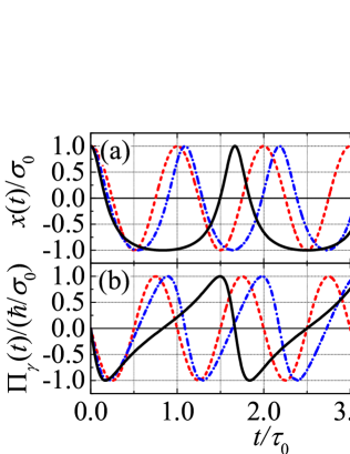
Figure 1: Temporal evolution of (a) position $x(t)$ and (b) linear pseudo-momentum $\Pi_{\gamma}(t)$ for a PDM classical oscillator with deformed phase $\theta_{\gamma}(t)$ given by Eq. (24) for $|\alpha_{\gamma}|=1/\sqrt{2}$ ($A=\sigma_{0}$) and deformation parameters $\gamma\sigma_{0}=0$ (dashed red), $0.4$ (dashed-dotted blue) and $0.8$ (solid black), (with $\tau_{0}=2\pi/\omega_{0}$ and $t_{0}=0$). (c) Complex number $\alpha_{\gamma}$, which corresponds to the state of the deformed oscillator, moves in an elliptic path. The abscissa and ordinate of $\alpha_{\gamma}(t)$ give $x(t)$ and $\Pi_{\gamma}(t)$, respectively.

III.2 Quantum oscillator with PDM

Considering the problem of the oscillator with PDM given by (3) under the quadratic potential $V(x)=\frac{1}{2}m_{0}\omega_{0}^{2}x^{2},$ the deformed Schrödinger equation is CostaFilho-Alencar-Skagerstam-AndradeJr-2013 ; Costa-Borges-2018

$$-\frac{\hbar^{2}}{2m_{0}}D_{\gamma}^{2}\varphi(x)+\frac{1}{2}m_{0}\omega_{0}^{2}x^{2}\varphi(x)=E\varphi(x).$$ (29)

In the deformed space $x_{\gamma}$, the Eq. (29) can be expressed in terms of a new field $\phi(x_{\gamma})=\varphi(x(x_{\gamma}))$ and it becomes the Schrödinger equation for the quantum Morse oscillator CostaFilho-Alencar-Skagerstam-AndradeJr-2013 ; Costa-Borges-2018

$$-\frac{\hbar^{2}}{2m_{0}}\frac{\textrm{d}^{2}{\phi}(x_{\gamma})}{\textrm{d}x_{\gamma}^{2}}+W_{\gamma}(e^{-\kappa_{\gamma}x_{\gamma}}-1)^{2}\phi({x_{\gamma}})=E\phi({x_{\gamma}}).$$ (30)

From the solutions of (30), we obtain the normalized eigenfunctions of the deformed oscillator

$$\psi_{n}(x) =\frac{\varphi_{n}(x)}{\sqrt{1+\gamma x}}$$

$$=(-1)^{n}\mathcal{N}_{n}\sqrt{2s}e^{-\frac{z(x)}{2}}[z(x)]^{\frac{\nu_{n}-1}{2}}L_{n}^{(\nu_{n})}(z(x))$$ (31)

for $x>-1/\gamma$ and $\psi_{n}(x)=0$ otherwise, where $z(x)=2s(1+\gamma x)$, $s=1/\gamma^{2}\sigma_{0}^{2}$, $\nu_{n}=2s-2n-1>0$, $\mathcal{N}_{n}^{2}=\nu_{n}\gamma\Gamma(n+1)/\Gamma(\nu_{n}+n+1)$ and $L_{n}^{(\nu)}(z)$ are the associated Laguerre polynomials. The energy eigenvalues are

$$E_{n}({\gamma})=\hbar\omega_{0}\left(n+\frac{1}{2}\right)-\frac{\hbar^{2}\gamma^{2}}{2m_{0}}\left(n+\frac{1}{2}\right)^{2}.$$ (32)

In particular, the eigenfunction for $n=0$ is

$$\psi_{0}(x)=\sqrt{\frac{2}{\gamma\sigma_{0}^{2}\Gamma\left(\frac{2}{\gamma^{2}\sigma_{0}^{2}}-1\right)}}e^{-\frac{z(x)}{2}}[z(x)]^{\frac{1}{\gamma^{2}\sigma_{0}^{2}}-1}.$$ (33)

Thus, instead of the standard case, whose ground state is a Gaussian package, the probability density $\rho_{0}(x)=|\psi_{0}(x)|^{2}$ behaves like a Gamma distribution

$$\rho_{0}(x)=\frac{2}{\gamma\sigma_{0}^{2}\Gamma(\lambda)}e^{-z(x)}[z(x)]^{\lambda-1},$$ (34)

with $\lambda=\frac{2}{\gamma^{2}\sigma_{0}^{2}}-1$ being the shape parameter. The ground state energy is $E_{0}({\gamma})=\frac{\hbar\omega_{0}}{2}-\frac{\hbar^{2}\gamma^{2}}{8m_{0}}.$

It is straightforward to verify that the expected values $\langle\hat{x}\rangle$, $\langle\hat{x}^{2}\rangle$, $\langle\hat{\Pi}_{\gamma}\rangle$ and $\langle\hat{\Pi}_{\gamma}^{2}\rangle$ for the $n$th state are given by CostaFilho-Alencar-Skagerstam-AndradeJr-2013 ; Costa-Borges-2018

$$\langle\hat{x}\rangle=-\gamma\sigma_{0}^{2}\left(n+\frac{1}{2}\right),$$ (35a)

$$\langle\hat{x}^{2}\rangle=\sigma_{0}^{2}\left(n+\frac{1}{2}\right),$$ (35b)

$$\langle\hat{\Pi}_{\gamma}\rangle=0,$$ (35c)

$$\langle\hat{\Pi}_{\gamma}^{2}\rangle=\frac{\hbar^{2}}{\sigma_{0}^{2}}\left(n+\frac{1}{2}\right)\left[1-\gamma^{2}\sigma_{0}^{2}\left(n+\frac{1}{2}\right)\right].$$ (35d)

The product of the uncertainties of the observables $\hat{x}$ and $\hat{\Pi}_{\gamma}$ is

$$\Delta x\Delta\Pi_{\gamma} =\hbar\left(n+\frac{1}{2}\right)\left[1-\gamma^{2}\sigma_{0}^{2}\left(n+\frac{1}{2}\right)\right]$$

$$=\hbar\left(n+\frac{1}{2}\right)(1+\gamma\langle\hat{x}\rangle),$$ (36)

which obeys the deformed uncertainty relation (15).

III.3 Supersymmetric quantum mechanics for deformed oscillator

The Hamiltonian operator (8) for the problem of a quadratic potential $V(\hat{x})=\frac{1}{2}m_{0}\omega_{0}\hat{x}^{2}$ can be factorized as

$$\hat{H}=\hbar\omega_{0}\hat{a}_{\gamma}^{\dagger}\hat{a}_{\gamma}+E_{0}({\gamma}),$$ (37)

with the annihilation and the creation operators given by

$$\hat{a}_{\gamma} =\sqrt{\frac{m_{0}\omega_{0}}{2\hbar}}\left[\hat{x}+\frac{\hbar\gamma}{m_{0}\omega_{0}}\hat{1}+\frac{i}{m_{0}\omega_{0}}(\hat{1}+\gamma\hat{x})\hat{p}\right]$$

$$=\sqrt{\frac{m_{0}\omega_{0}}{2\hbar}}\left(\hat{x}+\frac{\hbar\gamma}{2m_{0}\omega_{0}}\hat{1}+\frac{i}{m_{0}\omega_{0}}\hat{\Pi}_{\gamma}\right)$$ (38a)

and

$$\hat{a}_{\gamma}^{\dagger} =\sqrt{\frac{m_{0}\omega_{0}}{2\hbar}}\left[\hat{x}+\frac{\hbar\gamma}{m_{0}\omega_{0}}\hat{1}-\frac{i}{m_{0}\omega_{0}}\hat{p}(\hat{1}+\gamma\hat{x})\right]$$

$$=\sqrt{\frac{m_{0}\omega_{0}}{2\hbar}}\left(\hat{x}+\frac{\hbar\gamma}{2m_{0}\omega_{0}}\hat{1}-\frac{i}{m_{0}\omega_{0}}\hat{\Pi}_{\gamma}\right).$$ (38b)

We see that $\hat{a}_{\gamma}\psi_{0}(x)=0$, i.e., the ground state is annihilated by the operator $\hat{a}_{\gamma}$. Although $\hat{a}_{\gamma}$ and $\hat{a}_{\gamma}^{\dagger}$ factorize the Hamiltonian (8) for the quadratic potential, these not are the ladder operators since they satisfy the commutator $[\hat{a}_{\gamma},\hat{a}_{\gamma}^{\dagger}]=\hat{1}+\gamma\hat{x}.$ A deformed number operator $\hat{n}_{\gamma}=\hat{a}_{\gamma}^{\dagger}\hat{a}_{\gamma}$ leads to the expected value for $n$th state $\langle\hat{n}_{\gamma}\rangle=n\left[1-\frac{1}{2}\gamma^{2}\sigma_{0}^{2}(n+1)\right]\equiv[n_{\gamma}].$

We can straightforwardly verify that the operators (38) and (38) satisfy the commutation relations

$$[\hat{a}_{\gamma},\hat{a}_{\gamma}^{\dagger}\hat{a}_{\gamma}] =(\hat{1}+\gamma\hat{x})\hat{a}_{\gamma}$$

$$=\left(1-\gamma^{2}\sigma_{0}^{2}+\frac{\gamma\sigma_{0}}{\sqrt{2}}(\hat{a}_{\gamma}^{\dagger}+\hat{a}_{\gamma})\right)\hat{a}_{\gamma},$$ (39a)

$$[\hat{a}_{\gamma}^{\dagger},\hat{a}_{\gamma}^{\dagger}\hat{a}_{\gamma}] =-\hat{a}_{\gamma}^{\dagger}(\hat{1}+\gamma\hat{x})$$

$$=-\hat{a}_{\gamma}^{\dagger}\left(1-\gamma^{2}\sigma_{0}^{2}+\frac{\gamma\sigma_{0}}{\sqrt{2}}(\hat{a}_{\gamma}^{\dagger}+\hat{a}_{\gamma})\right).$$ (39b)

Similar to Eq. (20) for the classical analog, the Jacobi identify

$$[[\hat{a}_{\gamma},\hat{a}_{\gamma}^{\dagger}],\hat{H}]+[[\hat{H},\hat{a}_{\gamma}],\hat{a}_{\gamma}^{\dagger}]+[[\hat{a}_{\gamma}^{\dagger},\hat{H}],\hat{a}_{\gamma}]=0$$ (40)

is satisfied in quantum formalism, so that the operators $\hat{a}_{\gamma}$, $\hat{a}_{\gamma}^{\dagger}$ and $\hat{H}$ constitute a Lie algebra.

The supersymmetric partners Hamiltonian operators Plastino-etal-1999 ; Amir-Iqbal-2016 associated with $\hat{H}$ are

$$\hat{H}_{\scriptscriptstyle+}=\hbar\omega_{0}\hat{a}_{\gamma}^{\dagger}\hat{a}_{\gamma}=\frac{1}{2m_{0}}\hat{\Pi}_{\gamma}^{2}+V_{\scriptscriptstyle+}(\hat{x})$$ (41a)

and

$$\hat{H}_{\scriptscriptstyle-}=\hbar\omega_{0}\hat{a}_{\gamma}\hat{a}_{\gamma}^{\dagger}=\frac{1}{2m_{0}}\hat{\Pi}_{\gamma}^{2}+V_{\scriptscriptstyle-}(\hat{x}),$$ (41b)

whose potentials are $V_{\scriptscriptstyle+}(\hat{x})=\frac{1}{2}m_{0}\omega_{0}^{2}\hat{x}^{2}-E_{0}(\gamma)$ and $V_{\scriptscriptstyle-}(\hat{x})=\frac{1}{2}m_{0}\omega_{0}^{2}\hat{x}^{2}-E_{0}(\gamma)+\hbar\omega_{0}(\hat{1}+\gamma\hat{x}),$ respectively. That is, the potential of the partner operator $\hat{H}_{\scriptscriptstyle+}$ has only a shift equal to the energy of the ground state in relation to the original operator $\hat{H}$, while the potential of the partner operator $\hat{H}_{\scriptscriptstyle-}$ has also added a quanta of energy, $\hbar\omega_{0}$, and a term corresponding to a uniform electric field, $\hbar\omega_{0}\gamma\hat{x}$.

Denoting the eigenenergies and eigenfunctions equations of the partners operators as $\hat{H}_{\scriptscriptstyle+}\psi_{n}^{\scriptscriptstyle(+)}(x)=E_{n}^{\scriptscriptstyle(+)}\psi_{n}^{\scriptscriptstyle(+)}(x)$ and $\hat{H}_{\scriptscriptstyle-}\psi_{n}^{\scriptscriptstyle(-)}(x)=E_{n}^{\scriptscriptstyle(-)}\psi_{n}^{\scriptscriptstyle(-)}(x)$. Since $\hat{H}_{\scriptscriptstyle+}$ and $\hat{H}$ commute, then $\psi_{n}^{\scriptscriptstyle(+)}(x)=\psi_{n}(x)$. In addition, from wave function $\varphi_{n}^{\scriptscriptstyle(-)}(x)=\sqrt{1+\gamma x}\psi_{n}^{\scriptscriptstyle(-)}(x)$ and $\epsilon_{n}=E_{n}^{\scriptscriptstyle(-)}-\hbar\omega_{0}+E_{0}(\gamma),$ we arrive at the deformed Schrödinger equation

$$-\frac{\hbar^{2}}{2m_{0}}D_{\gamma}^{2}\varphi_{n}^{\scriptscriptstyle(-)}(x)+\frac{1}{2}m_{0}\omega_{0}x^{2}\varphi_{n}^{\scriptscriptstyle(-)}(x)+\hbar\omega_{0}\gamma x\varphi_{n}^{\scriptscriptstyle(-)}(x)=\epsilon_{n}\varphi_{n}^{\scriptscriptstyle(-)}(x).$$ (42)

From the change of variable $x\rightarrow x_{\gamma}$, Eq. (42) becomes also a Morse oscillator

$$-\frac{\hbar^{2}}{2m_{0}}\frac{\textrm{d}^{2}\phi_{n}^{\scriptscriptstyle(-)}(x_{\gamma})}{\textrm{d}x_{\gamma}^{2}}+\widetilde{W}_{\gamma}(e^{-\kappa_{\gamma}(x_{\gamma}-\delta_{\gamma})}-1)^{2}\phi_{n}^{\scriptscriptstyle(-)}(x_{\gamma})=\left(\epsilon_{n}+\frac{\hbar^{2}\gamma^{2}}{2m_{0}}\right)\phi_{n}^{\scriptscriptstyle(-)}(x_{\gamma}),$$ (43)

where $\phi_{n}^{\scriptscriptstyle(-)}(x_{\gamma})=\varphi_{n}^{\scriptscriptstyle(-)}(x(x_{\gamma})),$ $\widetilde{W}_{\gamma}=m_{0}\omega_{\gamma}^{2}/2\gamma^{2}$ is a shifted binding energy, and $\omega_{\gamma}=\omega_{0}(1-\gamma^{2}\sigma_{0}^{2})$ is the frequency of small oscillations around the equilibrium position $\delta_{\gamma}=\gamma^{-1}\ln(1-\gamma^{2}\sigma_{0}^{2})$. The solution of the above equations leads to the eigenfunctions

$$\psi_{n}^{\scriptscriptstyle(-)}(x) =\frac{\varphi_{n}^{\scriptscriptstyle(-)}(x)}{\sqrt{1+\gamma x}}$$

$$=(-1)^{n}\sqrt{2s}\widetilde{\mathcal{N}}_{n}e^{-\frac{z(x)}{2}}[z(x)]^{\frac{\widetilde{\nu}_{n}-1}{2}}L_{n}^{(\widetilde{\nu}_{n})}(z(x)),$$ (44)

with $\widetilde{\nu}_{n}=2s-2n-3$ and $\widetilde{\mathcal{N}}_{n}^{2}=\widetilde{\nu}_{n}\gamma\Gamma(n+1)/\Gamma(\widetilde{\nu}_{n}+n+1).$

The correspondence between the partner operators is established as follows

$$\hat{H}_{\scriptscriptstyle-}(\hat{a}_{\gamma}\psi_{n}^{\scriptscriptstyle(+)})=\hat{a}_{\gamma}(\hat{H}_{\scriptscriptstyle+}\psi_{n}^{\scriptscriptstyle(+)})=E_{n}^{\scriptscriptstyle(+)}(\hat{a}_{\gamma}\psi_{n}^{\scriptscriptstyle(+)})$$ (45a)

and

$$\hat{H}_{\scriptscriptstyle+}(\hat{a}_{\gamma}^{\dagger}\psi_{n}^{\scriptscriptstyle(-)})=\hat{a}_{\gamma}^{\dagger}(\hat{H}_{\scriptscriptstyle-}\psi_{n}^{\scriptscriptstyle(-)})=E_{n}^{\scriptscriptstyle(-)}(\hat{a}_{\gamma}^{\dagger}\psi_{n}^{\scriptscriptstyle(-)}),$$ (45b)

so that, $\hat{a}_{\gamma}\psi_{n}^{\scriptscriptstyle(+)}$ ($\hat{a}_{\gamma}^{\dagger}\psi_{n}^{\scriptscriptstyle(-)}$) is eigenfunction of $\hat{H}_{\scriptscriptstyle-}$ ($\hat{H}_{\scriptscriptstyle+}$). The energy spectra of the operators (41a) and (41b) obey the recurrence relation

$$E_{n}^{\scriptscriptstyle(+)}=E_{n-1}^{\scriptscriptstyle(-)}=E_{n}-E_{0}({\gamma})=\hbar\omega_{0}[n_{\gamma}]$$ (46)

and $E_{0}^{\scriptscriptstyle(+)}=0$. The eigenfunctions are related as

$$\hat{a}_{\gamma}\psi_{n}^{\scriptscriptstyle(+)}(x)=\left[\frac{E_{n}^{\scriptscriptstyle(+)}}{\hbar\omega_{0}}\right]^{1/2}\psi_{n-1}^{\scriptscriptstyle(-)}(x)$$ (47a)

and

$$\hat{a}_{\gamma}^{\dagger}\psi_{n}^{\scriptscriptstyle(-)}(x)=\left[\frac{E_{n}^{\scriptscriptstyle(-)}}{\hbar\omega_{0}}\right]^{1/2}\psi_{n+1}^{\scriptscriptstyle(+)}(x),$$ (47b)

in which can be verified from Eqs. (38), (46) and the expressions of $\psi_{n}^{\scriptscriptstyle(+)}(x)$ and $\psi_{n}^{\scriptscriptstyle(-)}(x)$ (see Appendix for more details).

The operators (38) are not the bosonic operators since

$$\hat{H}=\frac{\hbar\omega_{0}}{2}\{\hat{a}_{\gamma},\hat{a}_{\gamma}^{\dagger}\}-\frac{1}{2}\hbar\omega_{0}(\hat{1}+\gamma\hat{x})+E_{0}(\gamma).$$ (48)

However, the operators (38) can be used to obtain the supersymmetric Hamiltonian operator associated to the oscillator with PDM. In fact, considering the deformed bosonic operator $\hat{b}_{\gamma}=\hat{a}_{\gamma}-\frac{\gamma\sigma_{0}}{2\sqrt{2}}\hat{1}=\sqrt{\frac{m_{0}\omega_{0}}{2\hbar}}\left(\hat{x}+\frac{i}{m_{0}\omega_{0}}\hat{\Pi}_{\gamma}\right)$ and its adjoint $\hat{b}_{\gamma}^{\dagger}$, we get $\hat{H}$ expressed in terms of an anticommutator,

$$\hat{H}=\frac{\hbar\omega_{0}}{2}\{\hat{b}_{\gamma},\hat{b}_{\gamma}^{\dagger}\}.$$ (49)

The Hamiltonian (49) can be rewritten in terms of the deformed bosonic operators as

$$\hat{H}=\hbar\omega_{0}\left(\hat{b}_{\gamma}^{\dagger}\hat{b}_{\gamma}+\frac{1}{2}\right)+\frac{\hbar\omega_{0}\gamma\sigma_{0}}{2\sqrt{2}}(\hat{b}_{\gamma}^{\dagger}+\hat{b}_{\gamma}).$$ (50)

The first term in (50) corresponds to the Hamiltonian operator of a deformed oscillator, i.e., $\hat{h}_{\gamma}=\hbar\omega_{0}\left(\hat{b}_{\gamma}^{\dagger}\hat{b}_{\gamma}+\frac{1}{2}\right)$, while the second term is equivalent to an interaction potential of a uniform electric field due to the effect of the effective mass, $\hat{\mathcal{V}}_{\gamma}=\frac{1}{2}\hbar\omega_{0}\gamma\hat{x}$. Therefore, the supersymmetric Hamiltonian is

$$\hat{H}_{\textrm{ss}} =\hbar\omega_{0}\left(\begin{array}[]{cc}\hat{b}_{\gamma}^{\dagger}\hat{b}_{\gamma}&0\\ 0&\hat{b}_{\gamma}\hat{b}_{\gamma}^{\dagger}\end{array}\right)$$ (53)

$$=\left(\begin{array}[]{cc}\hat{H}-\frac{\hbar\omega_{0}}{2}(\hat{1}+\gamma\hat{x})&0\\ 0&\hat{H}+\frac{\hbar\omega_{0}}{2}(\hat{1}+\gamma\hat{x})\end{array}\right),$$ (56)

or more compactly, $\hat{H}_{\textrm{ss}}=\hat{H}-\left(\frac{\hbar\omega_{0}}{2}+\hat{\mathcal{V}}_{\gamma}\right)\widehat{\sigma}_{z},$ where $\widehat{\sigma}_{z}$ is the diagonal Pauli matrix.

III.4 Shape invariance

For the sake of completeness, let us consider the shape invariance technique to determine the wave functions and the energy spectrum for the deformed oscillator with PDM. The partner Hamiltonians are named shape invariants if they satisfy the integrability condition Plastino-etal-1999 ; Amir-Iqbal-2016

$$\hat{H}_{\scriptscriptstyle-}({\beta}_{j})-\hat{H}_{\scriptscriptstyle+}({\beta}_{j+1})=R({\beta}_{j}),$$ (57)

so that the set of parameters is related by a function $f$ such that $\beta_{j+1}=f(\beta_{j})$, and the remainder term $R(\beta_{j})$ is independent of the position and linear momentum operators. Since the partner operators differ only by an additive constant, their energy spectra and eigenstates are related respectively as

$$E_{n}^{\scriptscriptstyle(-)}({\beta}_{j}) =E_{n}^{\scriptscriptstyle(+)}({\beta}_{j+1})+R({\beta}_{j}),$$ (58a)

$$|\psi_{n}^{\scriptscriptstyle(-)}(\beta_{j})\rangle =|\psi_{n}^{\scriptscriptstyle(+)}(\beta_{j+1})\rangle=|\psi_{n}(\beta_{j+1})\rangle.$$ (58b)

The application of the shape invariance method to the deformed oscillator leads to change the intertwining operators (38) so that

$$\hat{a}_{\gamma}({\beta}) =\sqrt{\frac{m_{0}\omega_{0}}{2\hbar}}\left(\hat{x}+\frac{\beta\hbar\gamma}{2m_{0}\omega_{0}}\hat{1}+\frac{i}{m_{0}\omega_{0}}\hat{\Pi}_{\gamma}\right)$$ (59a)

and

$$\hat{a}_{\gamma}^{\dagger}({\beta}) =\sqrt{\frac{m_{0}\omega_{0}}{2\hbar}}\left(\hat{x}+\frac{\beta\hbar\gamma}{2m_{0}\omega_{0}}\hat{1}-\frac{i}{m_{0}\omega_{0}}\hat{\Pi}_{\gamma}\right).$$ (59b)

The creation and annihilation operators (38) are recovered as $\beta\rightarrow 1$. The supersymmetric partner Hamiltonians $\hat{H}_{\scriptscriptstyle+}({\beta})=\hbar\omega_{0}\hat{a}_{\gamma}^{\dagger}({\beta})\hat{a}_{\gamma}({\beta})$ and $\hat{H}_{\scriptscriptstyle-}({\beta})=\hbar\omega_{0}\hat{a}_{\gamma}({\beta})\hat{a}_{\gamma}^{\dagger}({\beta})$ are $\hat{H}_{\scriptscriptstyle\pm}=\frac{1}{2m_{0}}\hat{\Pi}_{\gamma}^{2}+V_{\scriptscriptstyle\pm}(\hat{x},\beta)$ with potentials $V_{\scriptscriptstyle\pm}(\hat{x},\beta)=V(\hat{x})\mp\frac{\hbar\omega_{0}}{2}[\hat{1}+(1\mp\beta)\gamma\hat{x}]+\frac{\beta^{2}\hbar^{2}\gamma^{2}}{8m_{0}}.$

Consequently, the integrability condition (57) becomes

$$\hbar\omega_{0}\hat{a}_{\gamma}({\beta}_{j})\hat{a}_{\gamma}^{\dagger}({\beta}_{j})-\hbar\omega_{0}\hat{a}_{\gamma}^{\dagger}({\beta_{j+1}})\hat{a}_{\gamma}({\beta_{j+1}})=R(\beta_{j}),$$ (60)

where the $\beta$-parameters satisfy a translational shape invariance $\beta_{j+1}=\beta_{j}+\eta$ with $\eta=2$, such that, $\beta_{n}=\beta+2(n-1)$ and $\beta_{1}\equiv\beta$. The remainder term is $R(\beta)=\hbar\omega_{0}\left[1-\frac{1}{2}\gamma^{2}\sigma_{0}^{2}(\beta+1)\right].$

The energy levels of the operator $\hat{H}_{\scriptscriptstyle+}({\beta})$ are obtained from $E_{n}^{\scriptscriptstyle(+)}({\beta})=\sum_{j=1}^{n}R({\beta}_{j}),$ with $E_{0}^{\scriptscriptstyle(+)}({\beta})=0.$ In this way, it is straightforwardly to verify that

$$E_{n}^{\scriptscriptstyle(+)}({\beta})=\hbar\omega_{0}n\left[1-\frac{\gamma^{2}\sigma_{0}^{2}}{2}(n+\beta)\right].$$ (61)

Thereby, the operator $\hat{H}(\beta)=\hbar\omega_{0}\hat{a}_{\gamma}^{\dagger}(\beta)\hat{a}_{\gamma}(\beta)+E_{0}(\gamma)$ has energy spectrum $E_{n}=E_{n}^{\scriptscriptstyle(+)}({\beta})+E_{0}(\gamma).$

The next step is to obtain the eigenfunctions using the shape invariance method. From Eq. (47a), the eigenstates of the oscillator satisfy the recurrence relation

$$|\psi_{n}({\beta}_{j})\rangle=\left[\frac{E_{n}^{\scriptscriptstyle(+)}}{\hbar\omega_{0}}\right]^{-1/2}\hat{a}_{\gamma}^{\dagger}({\beta}_{j+1})|\psi_{n-1}(\beta_{j+1})\rangle.$$ (62)

Applying $n$ interactions, it can be seen that

$$|\psi_{n}(\beta_{1})\rangle=\frac{1}{\sqrt{[n_{\gamma}({\beta})]!}}\hat{a}_{\gamma}^{\dagger}({\beta}_{1})\hat{a}_{\gamma}^{\dagger}({\beta}_{2})...\hat{a}_{\gamma}^{\dagger}({\beta}_{n})|\psi_{0}(\beta_{n+1})\rangle$$ (63)

with deformed factorial given by

$$[n_{\gamma}({\beta})]!=\prod_{j=1}^{n}\left[\frac{E_{j}^{\scriptscriptstyle(+)}({\beta})}{\hbar\omega_{0}}\right]=\frac{n!}{(2s)^{n}}\frac{\Gamma(2s+1-\beta-n)}{\Gamma(2s+1-\beta-2n)}.$$ (64)

The operator (59b) can be recasted as

$$\hat{a}_{\gamma}^{\dagger}({\beta})y(z) =\frac{1}{\sqrt{2s}}\left[-\frac{2s-\beta+1}{2}+\frac{z}{2}-z\frac{\textrm{d}}{\textrm{d}z}\right]y(z)$$

$$=-\frac{1}{\sqrt{2s}}\left[\frac{1}{g_{\scriptscriptstyle\beta}(z)}\left(z\frac{\textrm{d}}{\textrm{d}z}\right)g_{\scriptscriptstyle\beta}(z)\right]y(z)$$ (65)

with $y(z)$ being a generic function and $g_{\scriptscriptstyle\beta}(z(x))=e^{-\frac{z(x)}{2}}[z(x)]^{\frac{2s-\beta+1}{2}}.$ From that, we have

$$\prod_{j=1}^{n}\hat{a}_{\gamma}^{\dagger}({\beta}_{j})y(z)=\left(-\frac{1}{\sqrt{2s}}\right)^{n}\left[\frac{1}{g_{\scriptscriptstyle\beta}(z)}\left(z^{n}\frac{\textrm{d}^{n}}{\textrm{d}z^{n}}\right)g_{\scriptscriptstyle\beta}(z)\right]y(z).$$ (66)

The condition $\hat{a}_{\gamma}({\beta})|\psi_{0}({\beta})\rangle=0$ leads to the ground state

$$\psi_{0,\beta}(x)=\sqrt{\frac{2s\gamma}{\Gamma(2s-\beta)}}e^{-\frac{z(x)}{2}}[z(x)]^{\frac{2s-1-\beta}{2}}.$$ (67)

From Eqs. (63), (64), (66), (67) and Rodrigues’ formula for the associated Laguerre polynomials, $L_{n}^{(\nu)}(z)=\frac{1}{n!}e^{z}z^{-\nu}\times\frac{\textrm{d}^{n}}{\textrm{d}x^{n}}(z^{\nu+n}e^{-z}),$ we arrive at

$$\psi_{n,\beta}(x) =(-1)^{n}\sqrt{2s}\left[\frac{(\nu_{n}+1-\beta)\gamma\Gamma(n+1)}{\Gamma(\nu_{n}+2-\beta+n)}\right]^{1/2}e^{-\frac{z(x)}{2}}[z(x)]^{\frac{\nu_{n}-\beta}{2}}L_{n}^{(\nu_{n}+1-\beta)}(z(x)).$$ (68)

When the parameter $\beta\rightarrow 1$, the expression above reduces to the eigenfunctions (III.2).

Since the commutator between the $\hat{a}_{\gamma}(\beta)$ and $\hat{a}_{\gamma}^{\dagger}(\beta)$ depends on the position, they can not be chosen as ladder operators. However, the Hamiltonian operators $\hat{H}_{\scriptscriptstyle\pm}({\beta})$ are translational shape invariance, and in this case it is possible to define ladder operators as

$$\hat{L}_{\scriptscriptstyle-}({\beta})=\hat{\Lambda}^{\dagger}({\beta})\hat{a}_{\gamma}({\beta})\quad\textrm{and}\quad\hat{L}_{\scriptscriptstyle+}({\beta})=\hat{a}_{\gamma}^{\dagger}({\beta})\hat{\Lambda}({\beta})$$ (69)

with $\hat{\Lambda}^{\dagger}({\beta})$ and $\hat{\Lambda}({\beta})$ unitary translational operators on parameter $\beta$, which satisfying the reparametrization $\hat{\Lambda}(\beta)|\psi_{n}(\beta)\rangle=|\psi_{n}(\beta+\eta)\rangle.$ The translational operators $\hat{\Lambda}({\beta})$ and $\hat{\Lambda}^{\dagger}({\beta})$ are given respectively by Amir-Iqbal-2016

$$\hat{\Lambda}({\beta})=\exp\left(\eta\frac{\partial}{\partial\beta}\right)\ \ \textrm{and}\ \ \hat{\Lambda}^{\dagger}({\beta})=\exp\left(-\eta\frac{\partial}{\partial\beta}\right).$$ (70)

Once $\hat{\Lambda}^{\dagger}(\beta)\hat{\Lambda}(\beta)=\hat{1}$ the Hamiltonian operator (41a) preserves the form $\hat{H}_{\scriptscriptstyle+}({\beta})=\hat{H}(\beta)-E_{0}(\gamma)=\hbar\omega_{0}\hat{L}_{\scriptscriptstyle+}({\beta})\hat{L}_{\scriptscriptstyle-}({\beta}).$ From Eqs. (58) and (69), the action of the ladder operators on the ket vectors $|\psi_{n}\rangle$ is given by

$$\hat{L}_{\scriptscriptstyle-}|\psi_{n}({\beta})\rangle=\sqrt{n\left[1-\frac{\gamma^{2}\sigma_{0}^{2}}{2}(n+\beta)\right]}|\psi_{n-1}({\beta})\rangle,$$ (71a)

and

$$\hat{L}_{\scriptscriptstyle+}|\psi_{n}({\beta})\rangle=\sqrt{(n+1)\left[1-\frac{\gamma^{2}\sigma_{0}^{2}}{2}(n+1+\beta)\right]}|\psi_{n+1}({\beta})\rangle.$$ (71b)

Explicitly, the ladder operators have the form

$$\hat{L}_{\scriptscriptstyle-}({\beta})=e^{-\eta\frac{\partial}{\partial\beta}}\frac{1}{\sqrt{2}\sigma_{0}}\left[x+\frac{(\beta+1)\gamma\sigma_{0}^{2}}{2}+\sigma_{0}^{2}(1+\gamma x)\frac{\textrm{d}}{\textrm{d}x}\right],$$ (72a)

$$\hat{L}_{\scriptscriptstyle+}({\beta})=\frac{1}{\sqrt{2}\sigma_{0}}\left[x+\frac{(\beta-1)\gamma\sigma_{0}^{2}}{2}-\sigma_{0}^{2}(1+\gamma x)\frac{\textrm{d}}{\textrm{d}x}\right]e^{\eta\frac{\partial}{\partial\beta}}.$$ (72b)

After careful calculations, we have found that the effects of the ladder operators on wavefunctions are expressed as

$$\hat{L}_{\scriptscriptstyle\pm}({\beta})\psi_{n,\beta}(x)= \frac{1}{\sqrt{2}\sigma_{0}}\left\{\frac{1}{\gamma}\left[\frac{2s+1-\beta}{2s-2n\mp 1-\beta}-\frac{2s-2n\pm 1-\beta}{2s}\left(\frac{1}{1+\gamma x}\right)\right]\mp\sigma_{0}^{2}\frac{\textrm{d}}{\textrm{d}x}\right\}$$

$$\times\left[\sqrt{{\frac{(2s-2n\mp 2-{\beta})(2s-n\mp 1-{\beta})^{\pm 1}}{(2s-2n-{\beta})(2s-n-{\beta})^{\pm 1}}}}\frac{2s-2n\mp 1-{\beta}}{2s}\right]\psi_{n,\beta}(x).$$ (73)

The wavefunction for ground state (67) is obtained from $\hat{L}_{\scriptscriptstyle-}(\beta)\psi_{0,\beta}(x)=0,$ and the $n$th excited state is expressed by

$$\psi_{n,\beta}(x)=\frac{1}{\sqrt{[n_{\gamma}({\beta})]!}}[\hat{L}_{\scriptscriptstyle+}({\beta})]^{n}\psi_{0,\beta}(x).$$ (74)

A dynamic group associated with the ladder operators $\hat{L}_{\scriptscriptstyle-}$ and $\hat{L}_{\scriptscriptstyle+}$ can be built. For the case $\beta=1$, the action of the commutator $[\hat{L}_{\scriptscriptstyle-},\hat{L}_{\scriptscriptstyle+}]$ on the eigenfunctions is

$$[\hat{L}_{\scriptscriptstyle-},\hat{L}_{\scriptscriptstyle+}]\psi_{n}(x)=2l_{0}(n)\psi_{n}(x),$$ (75)

with the eigenvalues defined by $l_{0}(n)=\frac{1}{2}\left[1-\gamma^{2}\sigma_{0}^{2}(n+1)\right],$ so that we can introduce the operator $\hat{L}_{0}=\frac{1}{2}[1-\gamma^{2}\sigma_{0}^{2}(\hat{n}+1)].$ From the operators $\hat{M}_{\scriptscriptstyle\pm}=\sqrt{2s}\hat{L}_{\scriptscriptstyle\pm}$ and $\hat{M}_{0}=2s\hat{L}_{0}$, we get the following commutation relations

$$[\hat{M}_{\scriptscriptstyle+},\hat{M}_{\scriptscriptstyle-}]=2\hat{M}_{0}\quad\textrm{and}\quad[\hat{M}_{0},\hat{M}_{\scriptscriptstyle\pm}]=\pm\hat{M}_{\scriptscriptstyle\pm},$$ (76)

which corresponds to a Lie algebra $SU(1,1)$ for the deformed oscillator.

IV Coherent states

IV.1 Coherent states in position representation

Now we look for the quantum mechanical states for which the time evolution of the expected values of the position and the momentum operators are similar to their respective classic analogues of the deformed oscillator. Theses are the coherent states, whose classicity is expressed by the minimization of the uncertainty relationship (15). In order to achieve this goal we use the formalism introduced in Ref. Ruby-Senthilvelan-2010, for building coherent states of quantum systems with PDM. The deformed annihilation and creation operators (38) can be rewritten as

$$\hat{a}_{\gamma} =\sqrt{\frac{m_{0}\omega_{0}}{2\hbar}}\left[\hat{\Phi}_{\gamma}+\frac{\hbar}{m_{0}\omega_{0}}\sqrt[4]{\frac{m_{0}}{m(\hat{x})}}\frac{\textrm{d}}{\textrm{d}\hat{x}}\sqrt[4]{\frac{m_{0}}{m(\hat{x})}}\,\right]$$ (77a)

$$\hat{a}_{\gamma}^{\dagger} =\sqrt{\frac{m_{0}\omega_{0}}{2\hbar}}\left[\hat{\Phi}_{\gamma}-\frac{\hbar}{m_{0}\omega_{0}}\sqrt[4]{\frac{m_{0}}{m(\hat{x})}}\frac{\textrm{d}}{\textrm{d}\hat{x}}\sqrt[4]{\frac{m_{0}}{m(\hat{x})}}\,\right],$$ (77b)

with $\hat{\Phi}_{\gamma}=\hat{x}+\frac{\gamma\hbar}{2m_{0}\omega_{0}}\hat{1}$ the superpotential for the deformed oscillator.

In terms of the operators annihilation and creation, the superpotential and the linear pseudo-momentum have the similar form of the standard oscillator

$$\hat{\Phi}_{\gamma} =\sqrt{\frac{\hbar}{2m_{0}\omega_{0}}}\left(\hat{a}_{\gamma}+\hat{a}_{\gamma}^{\dagger}\right)$$ (78a)

$$\hat{\Pi}_{\gamma} =i\sqrt{\frac{m_{0}\hbar\omega_{0}}{2}}\left(\hat{a}_{\gamma}^{\dagger}-\hat{a}_{\gamma}\right),$$ (78b)

and they satisfy the deformed commutation relation $[\hat{\Phi}_{\gamma},\hat{\Pi}_{\gamma}]=i\hbar\frac{\Phi^{\prime}_{\gamma}(\hat{x})}{\sqrt{m(\hat{x})/m_{0}}}=i\hbar(\hat{1}+\gamma\hat{x}).$ Similar to the usual case, the superpotential is directly related to the wave function in the ground state. In the case of the deformed oscillator, it turns out that

$$\psi_{0}(x) =\mathcal{N}_{0}\sqrt[4]{\frac{m(x)}{m_{0}}}\exp\left[-\frac{1}{\sigma_{0}^{2}}\int^{x}\sqrt{\frac{m(y)}{m_{0}}}\Phi_{\gamma}(y)\textrm{d}y\right]$$

$$=\frac{\mathcal{N}_{0}}{\sqrt{1+\gamma x}}\exp\left[-\frac{1}{\sigma_{0}^{2}}\int^{x}\Phi_{\gamma}(y)\textrm{d}_{\gamma}y\right]$$ (79)

recovers Eq. (33) for the superpotential (78a).

Analogously as made by Glauber,Glauber-1963 the coherent states for a PDM particle are defined from the eigenvalues equation of the annihilation operatorRuby-Senthilvelan-2010

$$\hat{a}_{\gamma}|\alpha_{\gamma}\rangle=\alpha_{\gamma}|\alpha_{\gamma}\rangle,$$ (80)

where the wavefunction for the coherent states $\psi_{\textrm{cs}}(x)=\langle{x}|{\alpha_{\gamma}}\rangle$ in the position representation can be obtained by means of Eq. (38), such that

$$\frac{1}{\sqrt{2}\sigma_{0}}\left(x+\gamma\sigma_{0}^{2}+\sigma_{0}^{2}(1+\gamma{x})\frac{\textrm{d}}{\textrm{d}x}\right)\psi_{\textrm{cs}}(x)=\alpha_{\gamma}\psi_{\textrm{cs}}(x).$$ (81)

Solving Eq. (81), we arrived at a solution that is similar to the ground state (33)

$$\psi_{\textrm{cs}}(x)=\mathcal{N}_{\textrm{cs}}\sqrt{2s}e^{-\frac{z(x)}{2}}[z(x)]^{\frac{\sqrt{2}\alpha_{\gamma}}{\gamma\sigma_{0}}+\frac{1}{\gamma^{2}\sigma_{0}^{2}}-1},$$ (82)

with the normalization constant $\mathcal{N}_{\textrm{cs}}=\sqrt{\gamma/\Gamma(\lambda_{\textrm{cs}})}$ and $\lambda_{\textrm{cs}}=\frac{2}{\gamma^{2}\sigma_{0}^{2}}[1+\sqrt{2}\gamma\sigma_{0}\textrm{Re}(\alpha_{\gamma})]-1.$ The probability density for coherent states in position representation is the Gamma distribution (34) with $\lambda$ replaced by $\lambda_{\textrm{cs}}$, i.e., $\rho_{\textrm{cs}}(x)=\frac{2}{\gamma\sigma_{0}^{2}\Gamma(\lambda_{\textrm{cs}})}e^{-z(x)}[z(x)]^{\lambda_{\textrm{cs}}-1}.$

Alternatively, it is possible obtain the coherent states for PDM from the Perelomov approach,Ruby-Senthilvelan-2010 which is based on the definition of a displacement operator $\hat{\Xi}_{\gamma}$, such that $|\alpha_{\gamma}\rangle=\hat{\Xi}_{\gamma}(\alpha_{\gamma})|0\rangle,$ with $\hat{\Xi}_{\gamma}(\alpha_{\gamma})=e^{i\hat{\chi}_{\gamma}(\alpha_{\gamma})}$ and

$$\hat{\chi}_{\gamma}(\alpha_{\gamma})=-i\frac{\sqrt{2}\alpha_{\gamma}}{\sigma_{0}}\int^{\hat{x}}\sqrt{\frac{m(\hat{y})}{m_{0}}}\textrm{d}\hat{y}=-i\sqrt{2}\alpha_{\gamma}\frac{\hat{x}_{\gamma}}{\sigma_{0}}.$$ (83)

In fact,

$$\psi_{\textrm{cs}}(x) =\langle x|\hat{\Xi}_{\gamma}(\alpha_{\gamma})|0\rangle$$

$$\propto\exp\left[\sqrt{2}\alpha_{\gamma}\frac{\ln(1+\gamma x)}{\gamma\sigma_{0}}\right]\psi_{0}(x)$$

$$\propto e^{-\frac{1+\gamma x}{\gamma^{2}\sigma_{0}^{2}}}(1+\gamma x)^{\frac{\sqrt{2}\alpha_{\gamma}}{\gamma\sigma_{0}}+\frac{1}{\gamma^{2}\sigma_{0}^{2}}-1}$$ (84)

has the same form as Eq. (82). Likewise the usual case, the displacement operator satisfies $\hat{\Xi}_{\gamma}^{\dagger}(\alpha_{\gamma})\hat{a}_{\gamma}\hat{\Xi}_{\gamma}(\alpha_{\gamma})=\hat{a}_{\gamma}+\alpha_{\gamma}$ and $\hat{\Xi}_{\gamma}^{\dagger}(\alpha_{\gamma})\hat{a}_{\gamma}^{\dagger}\hat{\Xi}_{\gamma}(\alpha_{\gamma})=\hat{a}_{\gamma}^{\dagger}+\alpha_{\gamma}^{\ast},$ with $[\hat{\chi}(\alpha_{\gamma}),\hat{a}_{\gamma}]=i\alpha_{\gamma}$ and $[\hat{\chi}(\alpha_{\gamma}),\hat{a}_{\gamma}^{\dagger}]=i\alpha_{\gamma}^{\ast}$.

IV.2 Minimum relation of uncertainty with the coherent states

The expected values $\langle\hat{x}\rangle_{\textrm{cs}},$ $\langle\hat{x}^{2}\rangle_{\textrm{cs}},$ $\langle\hat{\Pi}_{\gamma}\rangle_{\textrm{cs}},$ $\langle\hat{\Pi}_{\gamma}^{2}\rangle_{\textrm{cs}}$ for coherent states are

$$\langle\hat{x}\rangle_{\textrm{cs}}=\frac{\sigma_{0}}{\sqrt{2}}(\alpha_{\gamma}^{\ast}+\alpha_{\gamma})-\frac{\gamma\sigma_{0}^{2}}{2},$$ (85a)

$$\langle\hat{x}^{2}\rangle_{\textrm{cs}}=\frac{\sigma_{0}^{2}}{2}\left[1+(\alpha_{\gamma}^{\ast}+\alpha_{\gamma})^{2}-\frac{\gamma\sigma_{0}}{\sqrt{2}}(\alpha_{\gamma}^{\ast}+\alpha_{\gamma})\right],$$ (85b)

$$\langle\hat{\Pi}_{\gamma}\rangle_{\textrm{cs}}=\frac{i\hbar}{\sqrt{2}\sigma_{0}}(\alpha_{\gamma}^{\ast}-\alpha_{\gamma}),$$ (85c)

$$\langle\hat{\Pi}_{\gamma}^{2}\rangle_{\textrm{cs}}=\frac{\hbar^{2}}{2\sigma_{0}^{2}}\left[1-(\alpha_{\gamma}^{\ast}-\alpha_{\gamma})^{2}+\frac{\gamma\sigma_{0}}{\sqrt{2}}(\alpha_{\gamma}^{\ast}+\alpha_{\gamma})-\frac{\gamma^{2}\sigma_{0}^{2}}{2}\right].$$ (85d)

From Eqs. (85a)–(85d), we obtain the uncertainty relations of the position and the linear pseudo-momentum $(\Delta x)_{\textrm{cs}}^{2}=\frac{\sigma_{0}^{2}}{2}(1+\gamma\langle\hat{x}\rangle_{\textrm{cs}})$ and $(\Delta\Pi_{\gamma})_{\textrm{cs}}^{2}=\frac{\hbar^{2}}{2\sigma_{0}^{2}}(1+\gamma\langle\hat{x}\rangle_{\textrm{cs}}).$ Therefore,

$$(\Delta x)_{\textrm{cs}}^{2}(\Delta\Pi_{\gamma})_{\textrm{cs}}^{2}=\frac{\hbar^{2}}{4}(1+\gamma\langle\hat{x}\rangle_{\textrm{cs}})^{2}=\frac{1}{4}|\langle[\hat{x},\hat{\Pi}_{\gamma}]\rangle|_{\textrm{cs}}^{2},$$ (86)

i.e., the coherent states $|\alpha_{\gamma}\rangle$ minimize the generalized uncertainty relation (15) for the deformed oscillator.

It is straightforward to verify that the expectation values of the momentum linear satisfy

$$\langle\hat{p}\rangle_{\textrm{cs}} =\frac{i\hbar}{{\sqrt{2}\sigma_{0}}}\frac{(\alpha_{\gamma}^{\ast}-\alpha_{\gamma})}{1+\frac{\gamma\sigma_{0}}{\sqrt{2}}(\alpha_{\gamma}^{\ast}+\alpha_{\gamma})-\gamma^{2}\sigma_{0}^{2}},$$ (87a)

$$\langle\hat{p}^{2}\rangle_{\textrm{cs}} =\frac{\hbar^{2}}{2\sigma_{0}^{2}}\frac{1}{1+\frac{\gamma\sigma_{0}}{\sqrt{2}}(\alpha_{\gamma}^{\ast}+\alpha_{\gamma})-\frac{3}{2}\gamma^{2}\sigma_{0}^{2}}\left[1-\frac{(\alpha_{\gamma}^{\ast}-\alpha_{\gamma})^{2}}{1+\frac{\gamma\sigma_{0}}{\sqrt{2}}(\alpha_{\gamma}^{\ast}+\alpha_{\gamma})-\gamma^{2}\sigma_{0}^{2}}\right].$$ (87b)

In Fig. 2, from Eqs. (85a), (85b) and (87) we plot the uncertainties of the position $(\Delta x)_{\textrm{cs}}$ and of the linear momentum $(\Delta p)_{\textrm{cs}}$ along with the product $(\Delta x)_{\textrm{cs}}(\Delta p)_{\textrm{cs}}$ for the coherent states $|\alpha_{\gamma}\rangle$ that belong to the region $|\textrm{Re}(\alpha_{\gamma})|,|\textrm{Im}(\alpha_{\gamma})|<2$. These three quantifiers result symmetric around $\textrm{Im}(\alpha_{\gamma})=0$. The plane of the uncertainty relation (corresponding to the standard case $\gamma\sigma_{0}=0$) becomes a curved surface as the deformation parameter $\gamma\sigma_{0}$ grows, thus allowing to distinguish the coherent states within the range analyzed.

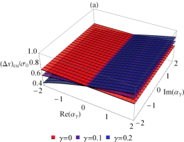
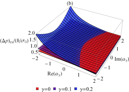
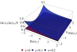
Figure 2: Uncertainties of (a) the position $(\Delta x)_{\textrm{cs}}$ and (b) the linear momentum $(\Delta p)_{\textrm{cs}}$ along with the product (c) $(\Delta x)_{\textrm{cs}}(\Delta p)_{\textrm{cs}}$ for the coherent states of the deformed oscillator in function of the complex number $\alpha_{\gamma}$, within the region $\{|\textrm{Re}(\alpha_{\gamma})|,|\textrm{Im}(\alpha_{\gamma})|<2\}$. The surfaces are illustrated for three representative values of the deformation parameter: $\gamma\sigma_{0}=0$ (usual case – red planes), $0.1$ (violet surfaces) and $0.2$ (blue surfaces).

IV.3 Quasi-classical states

Applying the time evolution operator $\hat{\mathcal{U}}(t,t_{0})=e^{-i\hat{H}(t-t_{0})/\hbar}$ on equation $|\alpha_{\gamma}(t_{0})\rangle=\hat{\Xi}_{\gamma}(\alpha_{\gamma}(t_{0}))|0\rangle,$ and considering the Heisenberg picture for displacement operator — $\hat{\Xi}_{\gamma}(t)=\hat{\mathcal{U}}(t,t_{0})\hat{\Xi}_{\gamma}(t_{0})\hat{\mathcal{U}}^{\dagger}(t,t_{0})$ — we get the coherent states at the instant $t$ is $|\alpha_{\gamma}(t)\rangle=e^{-iE_{0}(\gamma)(t-t_{0})/\hbar}\hat{\Xi}_{\gamma}(\alpha_{\gamma}(t))|0\rangle.$ So, to go from $|\alpha_{\gamma}(t_{0})\rangle$ to $|\alpha_{\gamma}(t)\rangle$, it is only necessary to replace $\alpha_{\gamma}(t_{0})$ by $\alpha_{\gamma}(t)$, and multiply the result by the phase factor $e^{-iE_{0}(\gamma)(t-t_{0})/\hbar}$. The corresponding probability density is given by

$$\rho_{\textrm{cs}}(x,t)=\frac{2}{\gamma\sigma^{2}\Gamma(\lambda_{\textrm{cs}}(t))}e^{-z(x)}[z(x)]^{\lambda_{\textrm{cs}}(t)-1}.$$ (88)

with shape parameter $\lambda_{\textrm{cs}}(t)=\frac{2}{\gamma^{2}\sigma_{0}^{2}}(1+\gamma A\cos\Theta_{\gamma}(t))-1$ and $\alpha_{\gamma}(t)=|\alpha_{\gamma}|e^{-i\Theta_{\gamma}(t)}$, in which $\Theta_{\gamma}(t)$ is a deformed phase for coherent states.

The time evolution of the operator $\hat{a}_{\gamma}$ is

$$\frac{\textrm{d}}{\textrm{d}t}\hat{a}_{\gamma}=\frac{1}{i\hbar}[\hat{a}_{\gamma},\hat{H}]=-i\omega_{0}(1+\gamma\hat{x})\hat{a}_{\gamma}.$$ (89)

Let $\hat{a}_{\gamma}(t)=\hat{a}_{\gamma}(t_{0})e^{-i\Theta_{\gamma}(t)}$, then we arrive at

$$\dot{\Theta}_{\gamma}(t)\hat{a}_{\gamma}(t)=\omega_{0}(\hat{1}+\gamma\hat{x}(t))\hat{a}_{\gamma}(t).$$ (90)

For coherent states, Eq. (90) can be rewritten as $\dot{\Theta}_{\gamma}(t)=\omega_{0}\left(1+\gamma A\cos\Theta_{\gamma}-\frac{\gamma^{2}\sigma_{0}^{2}}{2}\right).$ Analogously to the classical formalism, by integrating we obtain

$$\Theta_{\gamma}(t)=2\textrm{tan}^{-1}\left\{\sqrt{\frac{1+\gamma A_{\textrm{cs},\gamma}}{1-\gamma A_{\textrm{cs},\gamma}}}\textrm{tan}\left[\frac{1}{2}\Omega_{{\textrm{cs}},\gamma}(t-t_{0})\right]\right\}$$ (91)

with $\Theta_{\gamma}(t_{0})=0$ and the parameters modified $A_{\textrm{cs},\gamma}=A\left(1-\frac{\gamma^{2}\sigma_{0}^{2}}{2}\right)^{-1}$ and $\Omega_{\textrm{cs},\gamma}=\omega_{0}\sqrt{\left(1-\frac{\gamma^{2}\sigma_{0}^{2}}{2}\right)^{2}-\gamma^{2}A^{2}}.$ Figure 3 shows a comparison between the motion of the probability densities $\rho_{\textrm{cs}}(x,t)$ [Eq. (88)] for cases $\gamma\sigma_{0}=0$ (standard oscillator) and $0.4$.

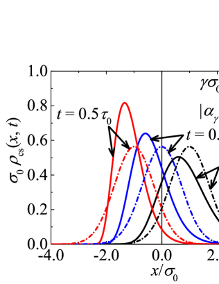
Figure 3: Motion of the probability density associated to the coherent states $|\alpha_{\gamma}\rangle$ of the deformed oscillator with the mass function $m(x)=m_{0}/(1+\gamma x)^{2}$ at the times $t=0$, $\tau_{0}/4$ and $\tau_{0}/2$ ($\tau_{0}=2\pi/\omega_{0}$) for $\gamma\sigma_{0}=0.4$ and $|\alpha_{\gamma}|=1/\sqrt{2}$. The usual case ($\gamma=0$, dashed line) is also illustrated for comparison.

Since $\textrm{Re}[\alpha_{\gamma}(t)]=|\alpha_{\gamma}|\cos\Theta_{\gamma}(t)$ and $\textrm{Im}[\alpha_{\gamma}(t)]=|\alpha_{\gamma}|\sin\Theta_{\gamma}(t),$ using Eqs. (85a) and (85c) we can express

$$\langle\hat{x}(t)\rangle_{\textrm{cs}} =A\cos{\Theta_{\gamma}}(t)-\frac{\gamma\sigma_{0}^{2}}{2},$$ (92a)

$$\langle\hat{\Pi}_{\gamma}(t)\rangle_{\textrm{cs}} =-m_{0}\omega_{0}A\sin{\Theta_{\gamma}}(t).$$ (92b)

As expected, the mean values of the position and the linear momentum (Eqs. (92a)–(92b)) evolve in the same way as their classic analogues. The position (92a) oscillates around an equilibrium position $x_{\textrm{eq},\gamma}=-\frac{\gamma\sigma_{0}^{2}}{2}$ due to the uniform electric field produced by the deformation of the space, whose force is $F_{\gamma}=-\textrm{d}\mathcal{V}_{\gamma}(x)/\textrm{d}x=-\frac{1}{2}\hbar\omega_{0}\gamma$. From Eq. (87a), the linear momentum is

$$\langle\hat{p}(t)\rangle_{\textrm{cs}}=-\frac{m_{0}\omega_{0}A\sin{\Theta_{\gamma}}(t)}{1+\gamma A\cos\Theta_{\gamma}(t)-\gamma^{2}\sigma_{0}^{2}}.$$ (93)

Figure 4 illustrates the phase space from the expected values (92a) and (93) for different values of $\gamma\sigma_{0}$. The paths are similar to corresponding classical analogues investigated previously in Ref. Costa-Borges-2018, . When $\gamma$ increases the center of the trajectory is shifted to the left.

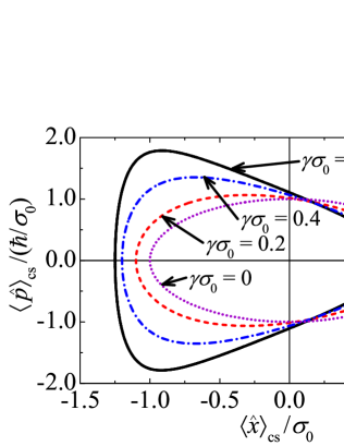
Figure 4: Phase space of the deformed oscillator associated to the coherent states $|\alpha_{\gamma}\rangle$ for $|\alpha_{\gamma}|=1/\sqrt{2}$ and deformation parameter $\gamma\sigma_{0}=0$ (dotted purple – usual case), $0.2$ (dashed red), $0.4$ (dashed-dotted blue) and $0.5$ (solid black).

In according to Ehrenfest’s theorem, the expected values of the superpotential and pseudo-momentum satisfy equations of motion identical to the classical analogues (28),

$$\left\{\begin{array}[]{rcl}\displaystyle\frac{1}{\sigma_{0}}\displaystyle\mathcal{D}_{\gamma}\langle\hat{\Phi}_{\gamma}(t)\rangle_{\textrm{cs}}&=&\displaystyle\frac{\sigma_{0}}{\hbar}\langle\hat{\Pi}_{\gamma}(t)\rangle_{\textrm{cs}}\\ \displaystyle\frac{\sigma_{0}}{\hbar}\displaystyle\mathcal{D}_{\gamma}\langle\hat{\Pi}_{\gamma}(t)\rangle_{\textrm{cs}}&=&\displaystyle-\frac{1}{\sigma_{0}}\langle\hat{\Phi}_{\gamma}(t)\rangle_{\textrm{cs}}\end{array}\right.$$ (94)

with $\mathcal{D}_{\gamma}(\,\cdot\,)=\frac{1}{1+\gamma\langle\hat{x}(t)\rangle_{\textrm{cs}}}\frac{\textrm{d}}{\textrm{d}t}(\,\cdot\,).$

The expected values of the Hamiltonian operator for coherent states are $\langle\hat{H}\rangle_{\textrm{cs}}=\mathcal{H}+E_{0}({\gamma}).$ In this way, we recover $|{\alpha}_{\gamma}|^{2}=\frac{\langle\hat{H}\rangle_{\textrm{cs}}-E_{0}(\gamma)}{\hbar\omega_{0}}=\frac{A^{2}}{2\sigma_{0}^{2}}.$ If $|\alpha_{\gamma}|$ is very large, then $A\gg\sigma_{0}$, and the quantum oscillator phase of the coherent states behave like the classical oscillator phase $\Theta_{\gamma}(t)\approx\theta_{\gamma}(t)$, as well as $\langle\hat{\Phi}_{\gamma}(t)\rangle_{\textrm{cs}}\rightarrow x(t)$ and $\langle\hat{\Pi}_{\gamma}(t)\rangle_{\textrm{cs}}\rightarrow\Pi_{\gamma}(t)$. As predicted, the dynamics of the coherent states for deformed oscillator are similar to the classical equations described Section II.

From $\alpha_{\gamma}(t)=|\alpha_{\gamma}|e^{-i\Theta_{\gamma}(t)}$, Eqs. (85a)–(85b), (87a)–(87b) and deformed phase (91), we plot in Fig. 5 the time evolution of the uncertainty relation [$(\Delta x)_{\textrm{cs}}(t)(\Delta p)_{\textrm{cs}}(t)$], along the uncertainties $(\Delta x)_{\textrm{cs}}(t)=\sqrt{\langle\hat{x}^{2}(t)\rangle_{\textrm{cs}}-\langle\hat{x}(t)\rangle_{\textrm{cs}}^{2}}$ and $(\Delta p)_{\textrm{cs}}(t)=\sqrt{\langle\hat{p}^{2}(t)\rangle_{\textrm{cs}}-\langle\hat{p}(t)\rangle_{\textrm{cs}}^{2}}$ for different values of $\gamma\sigma_{0}$. When $\gamma\rightarrow 0$ the oscillatory behavior on the uncertainties of the position and linear momentum disappears, so that they becomes $(\Delta x)_{\textrm{cs}}=\frac{\sigma_{0}}{\sqrt{2}}$ and $(\Delta p)_{\textrm{cs}}=\frac{\hbar}{\sqrt{2}\sigma_{0}}.$

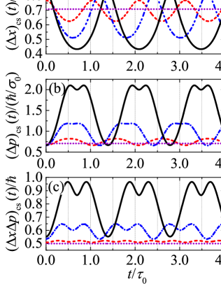
Figure 5: Time evolution of the uncertainties of (a) the position $(\Delta x)_{\textrm{cs}}(t)$ and (b) the linear momentum $(\Delta p)_{\textrm{cs}}(t)$, and (c) of the product $(\Delta x)_{\textrm{cs}}(t)(\Delta p)_{\textrm{cs}}(t)$ for the coherent states of the deformed oscillator with PDM, being $|\alpha_{\gamma}|=1/\sqrt{2}$ and deformation parameters $\gamma\sigma_{0}=0$ (dotted purple – usual case), $0.2$ (dashed red), $0.4$ (dashed-dotted blue) and $0.5$ (solid black).

V Final remarks

In this work, quantum and classical harmonic oscillators suitably deformed for accounting a particle with a position-dependent mass have been studied from the supersymmetric framework. We summarize our contributions as follows.

1. The classical and quantum Hamiltonians of the deformed harmonic oscillator are factorized in terms of their corresponding deformed ladder operators, the latter obtained by simply replacing the momentum by its deformed version.

2. The classical and quantum ladder operators preserve the Poisson and Lie brackets structure as well as the Jacobi identity.

3. The probability density of the ground state behaves like a Gamma distribution, as a result of the deformation, and it recovers the Gaussian package when the deformation tends to zero.

4. The position-dependent mass causes an additional term in the supersymmetric Hamiltonian, which is equivalent to introduce an uniform electric field in the $x$-direction. In turn, this feature could be used to represent uniform field interactions in terms of a PDM particle.

5. The deformed formalism preserves the structure of the shape invariant partner Hamiltonians in terms of the deformed ladder operators and the pseudo-momentum operator.

6. The coherent states of the deformed harmonic oscillator have the same structure than in the standard non-deformed case, by satisfying a minimum deformed uncertainty relation.

7. When the deformation is present the plane of the uncertainty relation transforms into a curved surface, thus serving as a distinguishability measure for the coherent states. The distinguishability becomes more pronounced as the the deformation parameter increases (Fig. 2).

The deformed oscillator carries pieces of information about the corrections of the generalized uncertainty principle (GUP). This is reflected by an increasing of the peaks in the temporal evolution of $\Delta x\Delta p$ along with an anharmonic oscillatory behavior, as the deformation parameter grows (Fig. 4). We also see that for some times the minimum of $\Delta x\Delta p$ is very close to the one corresponding to the standard case ($\gamma\sigma_{0}=0$), being almost independent of the deformation parameter for the range of values analyzed. This can be physically interpreted as if the GUP corrections are periodically cancelled for a particle with PDM being in a coherent state.

Overall, the deformation addressed in this paper, inspired by the formalism of the non-additive quantum mechanics CostaFilho-Almeida-Farias-AndradeJr-2011 ; Mazharimousavi-2012 ; Costa-Borges-2014 ; Barbagiovanni-Costafilho-2013 ; Barbagiovanni-2014 ; Costa-Gomez-Santos-2020 ; CostaFilho-Alencar-Skagerstam-AndradeJr-2013 ; Costa-Borges-2018 ; Costa-Gomez-Borges-2020 ; Tchoffo-Vubangsi-Fai-2014 ; Merad-etal_2019 ; Arda-Server ; Aguiar-Cunha-daCosta-CostaFilho-2020 ; CostaFilho-Oliveira-Aguiar-DaCosta-2021 contains a structural richness that allows modeling, ranging from effective position-dependent masses, uniform field interactions, deformed coherent states, to corrections of the GUP. In this sense, the use of other deformations could be helpful for modelling different scenarios.

The SUSY formalism applied to the deformed oscillator also opens new perspectives for the construction of other types of coherent states, such as the Barut-Girardello or Gazeau-Klauder formalisms.Gazeau-2009

Data availability

Data sharing is not applicable to this article as no new data were created or analyzed in this study.

Appendix

In the following, we demonstrate the expressions (47). Making the change of variable $x\rightarrow z=2(1+\gamma x)/\gamma^{2}\sigma_{0}^{2},$ so that the annihilation and creation operators on wavefunctions can be written as

$$\hat{a}_{\gamma}\psi_{n}^{\scriptscriptstyle(+)}=\frac{\gamma\sigma_{0}}{\sqrt{2}}\left(1-\frac{1}{\gamma^{2}\sigma_{0}^{2}}+\frac{z}{2}+z\frac{\textrm{d}}{\textrm{d}z}\right)\psi_{n}^{\scriptscriptstyle(+)},$$ (A1a)

$$\hat{a}_{\gamma}^{\dagger}\psi_{n}^{\scriptscriptstyle(-)}=\frac{\gamma\sigma_{0}}{\sqrt{2}}\left(-\frac{1}{\gamma^{2}\sigma_{0}^{2}}+\frac{z}{2}-z\frac{\textrm{d}}{\textrm{d}z}\right)\psi_{n}^{\scriptscriptstyle(-)}.$$ (A1b)

Substituting in Eq. (A1a) the eigenfunctions of the deformed oscillator in terms of the variable $z$, $\psi_{n}^{\scriptscriptstyle(+)}(x(z))=(-1)^{n}\sqrt{2s}{\mathcal{N}}_{n}e^{-\frac{z}{2}}z^{\frac{{\nu}_{n}-1}{2}}L_{n}^{({\nu}_{n})}(z),$ we get

$$\hat{a}_{\gamma}\psi_{n}^{\scriptscriptstyle(+)}=(-1)^{n}\mathcal{N}_{n}e^{-\frac{z}{2}}z^{\frac{{\nu}_{n}-1}{2}}\left(-nL_{n}^{({\nu}_{n})}(z)+z\frac{\textrm{d}L_{n}^{({\nu}_{n})}}{\textrm{d}z}\right).$$ (A2)

From the property of the Laguerre polynomials

$$z\frac{\textrm{d}L_{n}^{(\nu)}(z)}{\textrm{d}z} =(n+1)L_{n+1}^{(\nu)}(z)-(n+{\nu}+1-z)L_{n}^{(\nu)}(z),$$

$$=nL_{n}^{(\nu)}(z)-(n+{\nu})L_{n-1}^{(\nu)}(z),$$ (A3)

and using recurrence relationships $\mathcal{N}_{n}=\sqrt{\frac{n}{n+\nu_{n}}}\widetilde{\mathcal{N}}_{n-1}$ and $\nu_{n}=\widetilde{\nu}_{n-1},$ we arrive at

$$\hat{a}_{\gamma}\psi_{n}^{\scriptscriptstyle(+)}=(-1)^{n-1}\sqrt{n(n+{\nu}_{n})}\widetilde{\mathcal{N}}_{n-1}e^{-\frac{z}{2}}z^{\frac{\widetilde{\nu}_{n-1}-1}{2}}L_{n-1}^{(\widetilde{\nu}_{n-1})}(z).$$ (A4)

Since $\sqrt{n(n+\nu_{n})}=\sqrt{2sE_{n}^{\scriptscriptstyle(+)}/\hbar\omega_{0}},$ we obtain Eq. (47a).

Similarly, substituting in Eq. (A1b) the eigenfunctions $\psi_{n}^{\scriptscriptstyle(-)}(x(z))=(-1)^{n}\sqrt{2s}\widetilde{\mathcal{N}}_{n}e^{-\frac{z}{2}}z^{\frac{\widetilde{\nu}_{n}-1}{2}}L_{n}^{(\widetilde{\nu}_{n})}(z),$ leads us at

$$\hat{a}_{\gamma}^{\dagger}\psi_{n}^{\scriptscriptstyle(-)}=(-1)^{n+1}\widetilde{\mathcal{N}}_{n}e^{-\frac{z}{2}}z^{\frac{\widetilde{\nu}_{n}-1}{2}}\left[(n+\widetilde{\nu}_{n}+1-z)L_{n}^{(\widetilde{\nu}_{n})}(z)+z\frac{\textrm{d}L_{n}^{(\widetilde{\nu}_{n})}}{\textrm{d}z}\right].$$ (A5)

From Eq. (Appendix), $\widetilde{\mathcal{N}}_{n}=\sqrt{\frac{n+\nu_{n}-1}{n+1}}\mathcal{N}_{n+1}$ and $\widetilde{\nu}_{n}=\nu_{n+1},$ we obtain

$$\hat{a}_{\gamma}^{\dagger}\psi_{n}^{\scriptscriptstyle(-)}=(-1)^{n+1}\sqrt{(n+1)(n+{\nu}_{n}-1)}\mathcal{N}_{n+1}e^{-\frac{z}{2}}z^{\frac{{\nu}_{n+1}-1}{2}}L_{n+1}^{(\nu_{n+1})}(z).$$ (A6)

Since $\sqrt{(n+1)(n+{\nu}_{n}-1)}=\sqrt{2sE_{n}^{\scriptscriptstyle(-)}/\hbar\omega_{0}},$ we prove Eq. (A1b).

References

References

- (1) S. H. Dong, Factorization method in quantum mechanics (Springer, 2007).
- (2) E. Schrödinger, Proc. Roy. Irish Acad. 46, 9 (1940).
- (3) E. Witten, Nucl. Phys. B 188(3), 513 (1981).
- (4) F. Cooper and B. Freedman, Ann. Phys. 146(2), 262 (1983).
- (5) F. Cooper, A. Khare, and U. Sukhatme, Phys. Rep. 251, 267 (1995).
- (6) J. O. Rosas-Ortiz, J. Phys. A: Math. Gen. 31(50), 10163 (1998).
- (7) M. G. Benedict and B. Molnár, Phys. Rev. A 60(3), R1737 (1999).
- (8) G. R. P. Borges and E. Drigo Filho, Int. J. Mod. Phys 16(27), 4401 (2001).
- (9) C. B. Compean and M. Kirchbach, J. Phys. A: Math. Gen. 39(3), 547 (2005).
- (10) S. H. Dong and R. Lemus, Int. J. Quan. Chem. 86(3), 265 (2002).
- (11) E. Schrödinger, Naturwissenschaften 14(28), 664 (1926).
- (12) R. J. Glauber, Phys. Rev. 131(6), 2766 (1963).
- (13) J. R. Klauder, J. Math. Phys. 4(8), 1055 (1963).
- (14) J. R. Klauder, J. Math. Phys. 4(8), 1058 (1963).
- (15) E. C. G. Sudarshan, Phys. Rev. Lett. 10, 277 (1963).
- (16) J. P. Gazeau, Coherent states in quantum physics (Wiley-VCH, 2009).
- (17) G. Bastard, J. K. Furdyna, and J. Mycielsky, Phys. Rev. B 12, 4356 (1975).
- (18) O. von Roos, Phys. Rev. B 27, 7547 (1983).
- (19) D. J. BenDaniel and C. B. Duke, Phys. Rev. 152, 683 (1966).
- (20) T. Gora and F. Williams, Phys. Rev. 177, 1179 (1969).
- (21) Q. G. Zhu and H. Kroemer, Phys. Rev. B 27, 3519 (1983).
- (22) T. L. Li and K. J. Kuhn, Phys. Rev. B 47, 12760 (1993).
- (23) R. A. Morrow and K. R. Brownstein, Phys. Rev. B 30, 678 (1984).
- (24) O. Mustafa and S. H. Mazharimousavi, Int. J. Theor. Phys. 46, 1786 (2007).
- (25) R. Khordad, Physica B 406, 3911 (2011).
- (26) F. Arias de Saavedra, J. Boronat, A. Polls, and A. Fabrocini, Phys. Rev. B 50, 4248 (1994).
- (27) K. Bencheikh, K. Berkane and S. Bouizane, J. Phys. A: Math. Gen. 37 (45), 10719 (2004).
- (28) H. R. Christiansen and M. S. Cunha, J. Math. Phys. 55, 092102 (2014).
- (29) O. Cherroud, S. A. Yahiaoui, and M. Bentaiba, J. Math. Phys. 58, 063503 (2017).
- (30) G. Yanez-Navarro, G. H. Sun, T. Dytrych, K. D. Launey, S. H. Dong, and J. P. Draayer, Ann. Phys. 348 153 (2014).
- (31) M. L. Glasser, Phys. Lett. A 384, 126277 (2020).
- (32) C. S. Jia and A. de Souza Dutra, Ann. Phys. 323(3), 566 (2008).
- (33) M. F. Rañada, Phys. Lett. A 380, 2204 (2016).
- (34) M. Alimohammadi, H. Hassanabadi, and S. Zare, Nucl. Phys. A 960, 78 (2017).
- (35) A. L. de Jesus and A. G. Schmidt, J. Math. Phys. 60, 122102 (2019).
- (36) Z. Algadhi and O. Mustafa, Ann. Phys. 418, 168185 (2020).
- (37) A. R. Plastino, A. Rigo, M. Casas, F. Garcias, and A. Plastino, Phys. Rev. A 60(6), 4318 (1999).
- (38) N. Amir and S. Iqbal, J. Math. Phys. 57, 062105 (2016).
- (39) S. Karthiga, V. C. Ruby, and M. Senthilvelan, Phys. Lett. A 382(25), 1645 (2018).
- (40) R. Bravo and M. S. Plyushchay, Phys. Rev. D 93, 105023 (2016).
- (41) O. Mustafa, Phys. Lett. A 384, 126265 (2020).
- (42) V. Chithiika Ruby and M. Senthilvelan, J. Math. Phys. 51, 052106 (2010).
- (43) N. Amir and S. Iqbal, J. Math. Phys. 56, 062108 (2015).
- (44) N. Amir and S. Iqbal, Commun. Theor. Phys. 66, 615 (2016).
- (45) M. Tchoffo, F. B. Migueu, M. Vubangsi, and L. C. Fai, Heliyon 5(9), e02395 (2019).
- (46) A. Kempf, J. Math. Phys. 35, 4483 (1994).
- (47) S. Benczik, L. N. Chang, D. Minic and T. Takeuchi, Phys. Rev. A 72(1), 012104 (2005).
- (48) P. Pedram, Phys. Lett. B 714, 317 (2012).
- (49) S. Hossenfelder, Living Reviews in Relativity 16, 2 (2013).
- (50) P. Bosso, Phys. Rev. D 97(12), 126010 (2018).
- (51) R. N. Costa Filho, J. P. M. Braga, J. H. S. Lira, and J. S. Andrade Jr., Phys. Lett. B 755, 367 (2016).
- (52) B. G. da Costa, I. S. Gomez, and M. Portesi, J. Math. Phys. 61, 082105 (2020).
- (53) A. Merad, M. Aouachria, and H. Benzair, Few-Body Systems 61(4), 1 (2020).
- (54) R. N. Costa Filho, M. P. Almeida, G. A. Farias, and J. S. Andrade Jr., Phys. Rev. A 84, 050102(R) (2011).
- (55) S. H. Mazharimousavi, Phys. Rev. A 85, 034102 (2012).
- (56) B. G. da Costa and E. P. Borges, J. Math. Phys. 55, 062105 (2014).
- (57) E. G. Barbagiovanni et al., J. Appl. Phys. 115, 044311 (2014).
- (58) E. G. Barbagiovanni and R. N. Costa Filho, Physica E 63, 14 (2014).
- (59) B. G. da Costa, I. S. Gomez, and M. A. F. dos Santos, Europhys. Lett 129, 10003 (2020).
- (60) A. Arda and R. Sever, Few-Body Systems 56, 697 (2015).
- (61) R. N. Costa Filho, G. Alencar, B. S. Skagerstam, and J. S. Andrade Jr., Europhys. Lett. 101, 10009 (2013).
- (62) B. G. da Costa and E. P. Borges, J. Math. Phys. 59, 042101 (2018).
- (63) B. G. da Costa, I. S. Gomez, and E. P. Borges, Phys. Rev. E 102(6), 062105 (2020).
- (64) M. Tchoffo, M. Vubangsi and L. C. Fai, Physica Scripta 89 105201 (2014).
- (65) A. Merad, M. Aouachria, M. Merad, and T. Birkandan, Int. J. Mod. Phys. A, 34(32), 1950218 (2019).
- (66) V. Aguiar, S. M. Cunha, D. R. da Costa, R. N. Costa Filho Phys. Rev. B 102(23), 235404 (2020).
- (67) R. N. Costa Filho, S. F. S. Oliveira, V. Aguiar, and D. R. da Costa, Physica E 129, 114639 (2021).