Abstract

As Graph Neural Networks (GNNs) are increasingly being employed in critical real-world applications, several methods have been proposed in recent literature to explain the predictions of these models. However, there has been little to no work on systematically analyzing the reliability of these methods. Here, we introduce the first-ever theoretical analysis of the reliability of state-of-the-art GNN explanation methods. More specifically, we theoretically analyze the behavior of various state-of-the-art GNN explanation methods with respect to several desirable properties (e.g., faithfulness, stability, and fairness preservation) and establish upper bounds on the violation of these properties. We also empirically validate our theoretical results using extensive experimentation with nine real-world graph datasets. Our empirical results further shed light on several interesting insights about the behavior of state-of-the-art GNN explanation methods.

1 INTRODUCTION

Graph Neural Networks (GNNs) have emerged as powerful tools for effectively representing graph structured data, such as social, information, chemical, and biological networks. As these models are increasingly being employed in critical applications (e.g., drug repurposing (Zitnik et al., 2018), crime forecasting (Jin et al., 2020)), it becomes essential to ensure that the relevant stakeholders can understand and trust their functionality (Ying et al., 2019). Only if the stakeholders have a clear understanding of the behavior of these models, they can evaluate when and how much to rely on these models, and detect potential biases or errors in them. To this end, several approaches have been proposed in recent literature to explain the predictions of GNNs (Baldassarre and Azizpour, 2019; Faber et al., 2020; Huang et al., 2020; Lucic et al., 2021; Luo et al., 2020; Pope et al., 2019; Schlichtkrull et al., 2021; Vu and Thai, 2020; Ying et al., 2019). Based on the techniques they employ, these approaches can be broadly characterized into perturbation-based (Luo et al., 2020; Schlichtkrull et al., 2021; Ying et al., 2019), gradient-based (Simonyan et al., 2014; Sundararajan et al., 2017), and surrogate-based (Huang et al., 2020; Vu and Thai, 2020) methods (Yuan et al., 2020b).

While several classes of GNN explanation methods have been proposed in recent literature, there is little to no understanding as to which of these approaches are more effective than the others and/or if some of these approaches are better suited for certain kinds of real-world applications. This lack of understanding not only limits the applicability of GNN explanation methods in practice but also hinders the progress of research in graph XAI. More specifically, without such a deeper understanding, stakeholders in real-world settings may not be able to determine which approaches to employ, and researchers in the field may expend a lot of resources studying ineffective solutions. This lack of understanding mainly stems from the fact that there is very little work on systematically analyzing the reliability of various classes of state-of-the-art GNN explanation methods.

Few recent works have focused on empirically evaluating GNN explanation methods (Yuan et al., 2020b). For instance, Sanchez-Lengeling et al. (2020) focused on evaluating methods that output attributions (i.e., highlight input features influential to model predictions). They outlined various properties a GNN explanation method should satisfy — e.g., accuracy, faithfulness, and stability. Using these metrics, they empirically evaluated only gradient-based GNN explanation methods (e.g., SmoothGrad, GradCAM). More recently, Faber et al. (2021) highlighted the pitfalls of using arbitrary ground truth patterns in the data when evaluating GNN explanations as there may be a mismatch between these patterns and the GNN itself. They introduced three benchmark datasets to alleviate the aforementioned pitfalls. While these works make initial attempts at empirically evaluating GNN explanations, the metrics outlined are neither generalizable nor exhaustive. For example, most of the proposed metrics rely on the availability of ground truth explanations, thus severely limiting the kinds of datasets that can be used during evaluation. Those metrics do not account for fairness properties of explanations which are critical to applications like crime forecasting (Aivodji et al., 2019). Further, these works do not focus on theoretically analyzing the reliability or effectiveness of state-of-the-art GNN explanation methods.

Present work. In this work, we introduce the first ever theoretical analysis of the reliability of state-of-the-art GNN explanation methods. More specifically, we analyze the behavior of various GNN explanation methods w.r.t. several key desirable properties such as faithfulness (i.e., faithfully mimicking the predictions of the underlying model), stability (to small changes in the input), and fairness preservation (i.e., preserving the (un)fairness of the underlying model). While we leverage existing notions of faithfulness and stability outlined in prior literature, we introduce the notion of fairness preservation for GNN explanations for the first time in this work. As GNNs are increasingly being deployed in domains such as criminal justice and financial lending, it becomes critical to ensure that the GNN explanations preserve the fairness properties of the underlying GNN models. For instance, if a GNN model is biased against a protected group (e.g., violates the notion of statistical parity), then the corresponding explanation should reflect that.

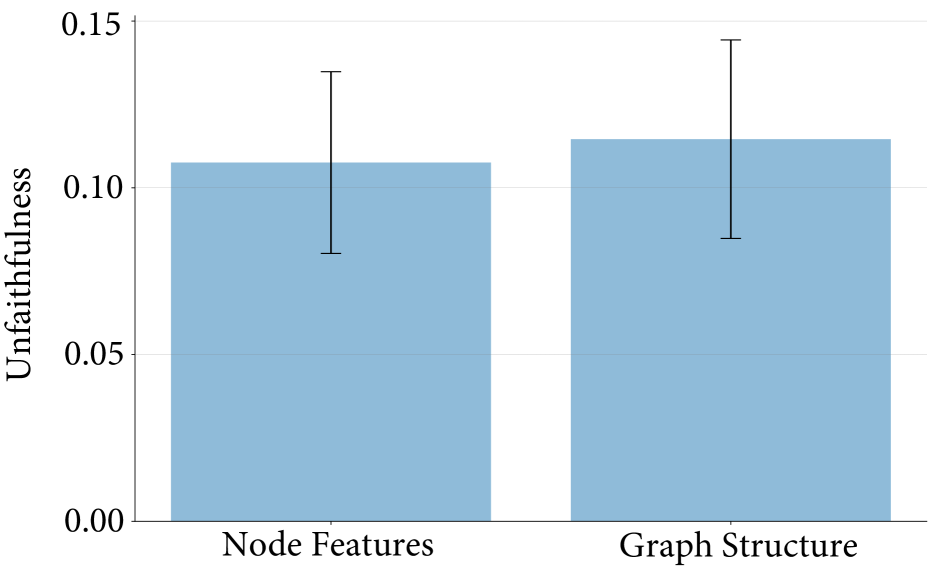
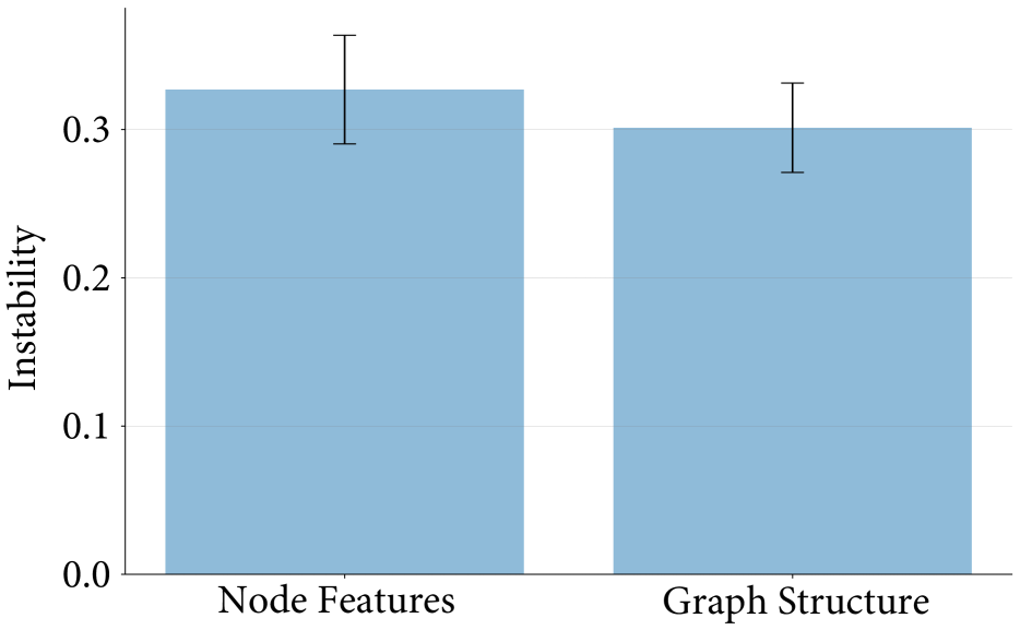
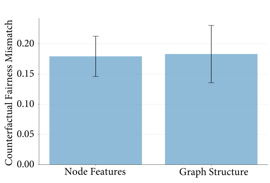
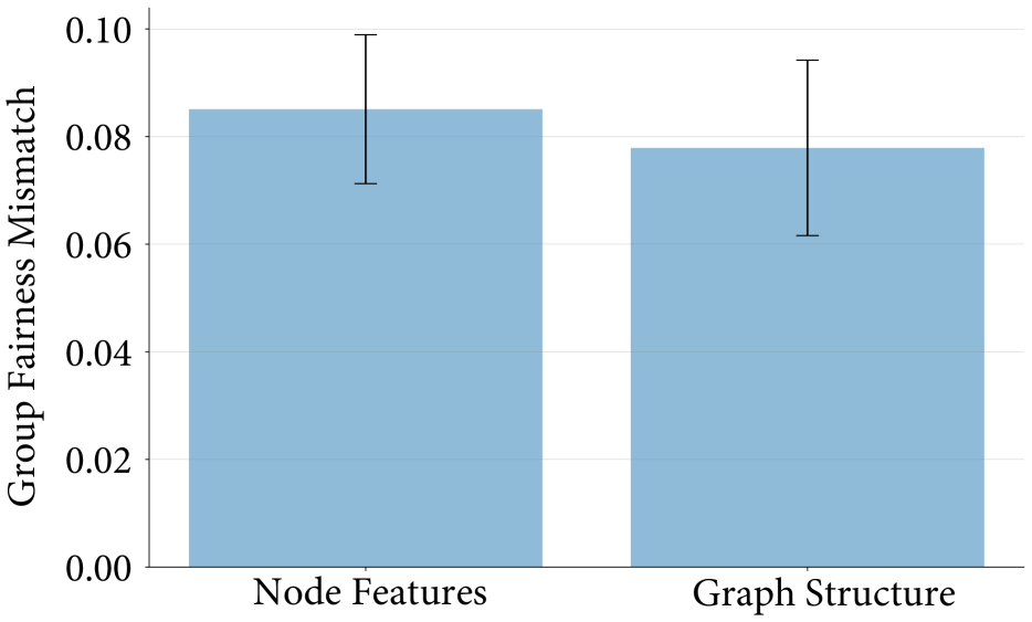
Figure 4: Shown are bar plots with mean values and standard errors of computed metrics for explanation methods generating node- (VanillaGrad, Integrated Gradients, GraphLIME, GNNExplainer) and graph-level (PGMExplainer, GraphMASK, PGExplainer) explanations across all datasets. We observe that graph structure-based explanations are more stable than node feature explanations, but performs on par in terms of other properties.

We formalize the above properties such that they do not rely on the availability of ground truth explanations and are therefore more generalizable to different domains and datasets. We then leverage these formalisms to establish theoretical upper bounds on the violation of the aforementioned properties for various state-of-the-art GNN explanation methods (Sec. 3). To carry out our theoretical analysis, we leverage the notion of Lipschitz continuity (Theorems 2-7) and employ concepts from information theory and probability theory such as data processing inequalities (Theorems 1-8) and total variation distance (Theorem 8). We also perform an extensive empirical evaluation with GNN explanation methods on nine real-world datasets and multiple learning tasks (i.e., node classification, link prediction and graph classification). Our empirical results validate our theoretical bounds and also unearth some critical insights about the behavior of state-of-the-art GNN explanation methods, 1) Gradient-based methods exhibit poor performance w.r.t. faithfulness and stability, but perform quite well w.r.t. counterfactual fairness; perturbation-based methods, on the other hand, exhibit the best performance at preserving group fairness (Fig. C.1), 2) Random baselines (particularly random edge baseline) perform either on par or sometimes even better than state-of-the-art GNN explanation methods (Fig. 6) w.r.t. faithfulness and group fairness preservation, and 3) on average across all datasets and all our key properties, explanations comprising of graph structures perform slightly better than those that comprise of node features (Fig. 4).

2 RELATED WORK

This paper builds upon a wealth of previous research at the intersection of explanation methods, graph neural networks, and systematic evaluation of explanations.

Explanation methods for GNNs. GNNs specify non-linear transformation functions that map graph structures (nodes, edges or entire graphs) into compact vector embeddings (Li et al., 2021). A variety of GNN architectures have been designed  (Pareja et al., 2020; Yun et al., 2019; Zitnik et al., 2018), and recent research has focused on developing methods to explain GNN predictions (Baldassarre and Azizpour, 2019; Pope et al., 2019; Ying et al., 2019; Huang et al., 2020; Luo et al., 2020; Vu and Thai, 2020; Schlichtkrull et al., 2021; Chen et al., 2021; Han et al., 2021). Early methods developed graph analogs of gradient-based methods from computer vision literature, including gradient heatmaps (Simonyan et al., 2014) and integrated gradients (Sundararajan et al., 2017). Recently, perturbation-based methods (Ying et al., 2019; Luo et al., 2020; Schlichtkrull et al., 2021) explain GNN predictions by observing the change in model predictions w.r.t. different input perturbations to study node and edge importance. Finally, surrogate-based methods (Huang et al., 2020; Vu and Thai, 2020) fit an interpretable model to local neighborhoods of the node such that the model captures the GNN’s behavior in the local vicinity of target nodes. See Appendix A for a detailed overview of the explanation methods.

Evaluation of GNN explanation methods. Empirical studies of deep neural network explanations evaluated methods and designed benchmarks for image, text, audio, time series, and sensory datasets (Jeyakumar et al., 2020; Liu et al., 2021; Arya et al., 2019; Fauvel et al., 2020; DeYoung et al., 2020; Amparore et al., 2021). However, due to the relative infancy of GNN explainability as a field, rigorous analyses of GNN explanation methods are very limited. While few works such as Sanchez-Lengeling et al. (2020); Yuan et al. (2020b); Faber et al. (2021) make initial attempts at empirically evaluating GNN explanation methods, the metrics outlined are neither generalizable nor exhaustive. For instance, most of the proposed metrics rely on the availability of ground truth explanations, thus severely limiting the kinds of datasets that can be used for evaluation. The proposed metrics also do not account for fairness properties of explanations which are critical to applications such as crime forecasting (Aivodji et al., 2019). Furthermore, despite few preliminary attempts at theoretical analysis of generic XAI techniques such as LIME and SmoothGrad (Chen et al., 2018; Agarwal et al., 2021b; Garreau and Luxburg, 2020), no theoretical analysis of GNN explanation methods has been attempted.

3 THEORETICAL ANALYSIS OF GNN EXPLANATION METHODS

In this section, we theoretically analyze the reliability of various state-of-the-art GNN explanation methods. We first outline and formalize the key desirable properties that capture the reliability of a given GNN explanation, namely, faithfulness, stability, and fairness preservation. More specifically, we posit that a reliable GNN explanation should faithfully mimic the predictions of the underlying GNN model, preserve critical model characteristics such as (un)fairness of the underlying model, and exhibit stability to small input perturbations. While we adopt existing notions of faithfulness and stability outlined in prior literature, we introduce and define the notion of fairness preservation for GNN explanations for the first time in this work. We then leverage these formalisms to derive upper bounds on the violation of the aforementioned properties for several GNN explanation methods.

Notation: Graphs and GNNs. Let $\mathcal{G}{=}(\mathcal{V},\mathcal{E},\mathbf{X})$ denote an undirected and unweighted graph comprising of a set of nodes $\mathcal{V}$, a set of edges $\mathcal{E}$, and a set of node feature vectors $\mathbf{X}{=}\{\mathbf{x}_{1},\dots,\mathbf{x}_{N}\}$ corresponding to nodes in $\mathcal{V}$, where $\mathbf{x}_{u}{\in}\mathbb{R}^{M}$. Let $N{=}|\mathcal{V}|$ denote the number of nodes in the graph and $\mathbf{A}\in\mathbb{R}^{N\times N}$ be the adjacency matrix, where element $\mathbf{A}_{ij}{=}1$ if nodes $i$ and $j$ are connected by some edge in $\mathcal{E}$, and $\mathbf{A}_{ij}{=}0$ otherwise. We use $\mathcal{N}_{u}$ to denote the 1-hop neighbors of node $u$ excluding itself. Without loss of generality, we focus on the node classification task and use $f$ to denote a GNN model trained to predict node labels. Note that the metrics we consider in this work can also be applied to other graph machine learning tasks (e.g., link prediction and graph prediction) as we demonstrate in Sec. 4. The GNN model’s prediction for node $u$ is given by $\mathbf{\hat{y}}_{u}{=}f(\mathcal{G}_{u})$, where $\mathcal{G}_{u}$ is the computation graph for node $u$ and $\mathbf{\hat{y}}_{u}{\in}[0,1]^{C}$. The associated adjacency matrix and node attributes for $\mathcal{G}_{u}$ are denoted by $\mathbf{A}_{u}{\in}\{0,1\}^{N\times N}$ (an element in this matrix has the value $1$ if it corresponds to an edge connecting node $u$ and some node in $\mathcal{N}_{u}$; otherwise it is set to $0$) and $\mathbf{X}_{u}{=}\{\mathbf{x}_{i}|i\in\{u,\mathcal{N}_{u}\}\}$ respectively. Also, $\hat{y}_{u}{=}\operatorname*{arg\,max}_{c}\mathbf{\hat{y}}_{u}$ is the predicted label, where $\hat{y}_{u}\in\{0,1,\dots,C-1\}$ and $C$ is the number of classes.

Notation: GNN explanations. In this work, we focus on instance level explanations which are the most popular class of explanations studied in GNN literature. Instance level explanations, as the name suggests, explain model predictions associated with individual entities (e.g., nodes) in the graph (and do not capture the global behavior of the entire GNN model). For instance, the explanation $\mathbf{E}_{u}$ corresponding to node $u$ comprises of a subset of node features and a subset of edges that influence the prediction of node $u$, i.e., $\hat{y}_{u}$. In particular, the explanation $\mathbf{E}_{u}$ consists of a discrete node feature mask $\mathbf{r}_{u}{\in}\{0,1\}^{M}$ and/or a discrete edge mask $\mathbf{R}_{u}{\in}\{0,1\}^{N{\times}N}$. An element in $\mathbf{r}_{u}$ or $\mathbf{R}_{u}$ takes the value $1$ if the corresponding node feature or edge (respectively) influences the prediction (and is therefore important), and is set to $0$ otherwise. We use $t(\mathbf{E}_{u},\mathcal{G}_{u})$ to denote a masking function which zeroes out all those node features and incident edges of $u$ that are not deemed as important by the explanation $\mathbf{E}_{u}$, i.e., $t(\mathbf{E}_{u},\mathcal{G}_{u})$ updates the node attributes and adjacency matrix corresponding to $\mathcal{G}_{u}$ as follows: $\mathbf{X}_{u}{=}\{\mathbf{x}_{u}\circ\mathbf{r}_{u}\}\cup\{\mathbf{x}_{i}|i\in\mathcal{N}_{u}\}$ and $\mathbf{A}_{u}{=}\mathbf{R}_{u}\circ\mathbf{A}_{u}$. Finally, we use $\hat{y}^{E}_{u}{=}f(t(\mathbf{E}_{u},\mathcal{G}_{u}))$ to denote the prediction label output by $f$ for node $u$ when the masked subgraph is provided as the input.

3.1 Theoretical Guarantees on Faithfulness

A reliable explanation should highlight the key node/edge features that the underlying GNN leverages to make a prediction. In a GNN’s neural message-passing scheme, every node has access to a local view of the graph created by propagating neural messages (embeddings) along edges in the node’s local neighborhood (Vignac et al., 2020). Following Pope et al. (2019) and Yuan et al. (2020b), we evaluate the faithfulness of the explanation corresponding to any given node $u$ by leveraging both its features as well as the incident edges. Formally, we say that an explanation $\mathbf{E}_{u}$ corresponding to a node $u$ is faithful if it accurately captures the behavior of the underlying model $f$ in the local region around $u$. To operationalize this, we first generate the local region around $u$ by constructing a set $\mathcal{K}$ of nodes comprising of node $u$ and its perturbations. These perturbations are generated by making infinitesimally small changes to its node features and/or rewiring the edges incident on node $u$ with a small probability. Next, we obtain the model predictions as well as explanation $\mathbf{E}_{u}$’s predictions for node $u$ and all its perturbations. Note that the explanation’s predictions can be obtained by first using the mapping function $t$, which takes an explanation mask and applies it to any given node and its subgraph (See Notation on GNN explanations above) to generate a new masked subgraph, which is then passed as input to the model $f$ to obtain a prediction. The average difference between the model and explanation predictions for all the nodes in $\mathcal{K}$ will provide us with an estimate of how unfaithful the explanation $\mathbf{E}_{u}$ is. The smaller this estimate, the more faithful the explanation $\mathbf{E}_{u}$.

Definition 1 (Faithfulness). Given a set $\mathcal{K}$ comprising of a node $u$ and its perturbations, an explanation $\mathbf{E}_{u}$ corresponding to node $u$ is said to be faithful if:

$$\frac{1}{|\mathcal{K}|}\sum_{u^{\prime}\in\mathcal{K}}||f(\mathcal{G}_{u^{\prime}})-f(t(\mathbf{E}_{u},\mathcal{G}_{u^{\prime}}))||_{2}\leq\delta,$$ (1)

where $\mathcal{G}_{u^{\prime}}$ denotes a subgraph of node $u^{\prime}$ and $\delta$ is an infinitesimally small constant. Note that the left hand side of Eqn. 1 is a measure of unfaithfulness of the explanation $\mathbf{E}_{u}$. So, higher values indicate higher degree of unfaithfulness.

Now we derive upper bounds on unfaithfulness of explanations output by GNN explanation methods.

Theorem 1. Given a node $u$ and a set $\mathcal{K}$ of node perturbations, the unfaithfulness (Sec. 3.1, Eqn. 1) of its explanation $\mathbf{E}_{u}$ can be bounded as follows:

$$\frac{1}{|\mathcal{K}|}\sum_{u^{\prime}\in\mathcal{K}}||f(\mathcal{G}_{u^{\prime}})-f(t(\mathbf{E}_{u},\mathcal{G}_{u^{\prime}}))||_{2}\leq\gamma\leavevmode\nobreak\ \frac{(1{+}|\mathcal{K}|)}{|\mathcal{K}|}\leavevmode\nobreak\ ||\Delta||_{2},$$

where $f(\mathcal{G}_{u^{\prime}}){=}\mathbf{\hat{y}}_{u^{\prime}}$ are softmax predictions using original graph attributes, $f(t(\mathbf{E}_{u},\mathcal{G}_{u^{\prime}})){=}\mathbf{\hat{y}}_{u^{\prime}}^{E}$ are softmax predictions using important attributes identified by $\mathbf{E}_{u}$, $\gamma$ is the product of the Lipschitz constants for GNN’s activation function and layer weights, and $\Delta$ represents the embedding difference for node $u$ when we exclude unnecessary nodes/node features/edges as identified by an explanation.

Proof Sketch.  In Theorem 1, the bound estimates an explanation’s unfaithfulness and is tight if the Lipschitz constant of the activation functions and $\ell_{p}$-norm of the GNN weights are bounded. The theorem demonstrates that the bound is dependent not only on the output explanation but also on the weights of the GNN and is small when the difference between the embeddings using $\mathbf{E}_{u}$ (see notations) is small or for GNN layers having smaller Lipschitz constant values.

We show that unfaithfulness of a node feature explanation (like GraphLIME) is bounded by $\gamma_{11}\frac{1{+}|\mathcal{K}|}{|\mathcal{K}|}||(\mathbf{1}{-}\mathbf{r}_{u})\circ\mathbf{x}_{u}||_{2}$, where $\gamma_{11}$ is the product of the Lipschitz constant for GNN’s activation function, weights of the last classification layer and self-attention weight of node $u$ across all GNN layers, and $\Delta$ for GraphLIME is $(\mathbf{1}{-}\mathbf{r}_{u})\circ\mathbf{x}_{u}$ representing the difference in node $u$’s features when we exclude the unimportant node features identified by the explanation. Similarly, for an edge-level explanations (like GraphMASK), the unfaithfulness is bounded by $\gamma_{12}\frac{(1{+}|\mathcal{K}|)}{|\mathcal{K}|}||\Delta_{\mathbf{x}_{v}}||_{2}$, where $\gamma_{12}$ is similar to $\gamma_{11}$ but uses weights associated with $u$’s immediate neighbors instead of self-attention weight and $\Delta_{\mathbf{x}_{v}}$ is the difference between embeddings of $u$’s neighbors where we exclude unnecessary edges as identified by the GraphMASK explanation. See Appendix B.1 for more details.

3.2 Theoretical Guarantees on Stability

Another key trait of a reliable explanation is that it should exhibit stability, i.e., infinitesimally small perturbations to an instance (which do not affect its model prediction) should not change its explanation drastically (Lakkaraju et al., 2020; Yuan et al., 2020b). To this end, we use the definition of stability outlined in Yuan et al. (2020b). An explanation $\mathbf{E}_{u}$ for node $u$’s prediction is considered stable if the explanations corresponding to $u$ (i.e., $\mathbf{E}_{u}$) and its perturbation $u^{\prime}$ (denoted by $\mathbf{E}_{u^{\prime}}$) are similar. Here, the perturbation $u^{\prime}$ is generated in the same way as above by rewiring the edges incident on $u$ with a small probability and/or making small changes to its node features.

Definition 2 (Stability). Given a node $u$ and its perturbation $u^{\prime}$, an explanation $\mathbf{E}_{u}$ corresponding to node $u$ is said to be stable if:

$$\mathcal{D}\big{(}\mathbf{E}_{u},\mathbf{E}_{u^{\prime}}\big{)}\leq\delta,$$ (2)

where $\mathbf{E}_{u^{\prime}}$ is the explanation for $u^{\prime}$, $\mathcal{D}(\cdot)$ computes distance between two explanations, and $\delta$ is an infinitesimally small constant. The left side of Eqn. 2 measures instability of the explanation $\mathbf{E}_{u}$ and higher values indicate higher instability.

Now, we take a representative explanation method for each class of gradient-based (VanillaGrad (Simonyan et al., 2014)), perturbation-based (GraphMASK (Schlichtkrull et al., 2021)), and surrogate-based (GraphLIME (Huang et al., 2020)) methods and derive bounds on the instability of their explanations.

Theorem 2 (VanillaGrad). Given a non-linear activation function $\sigma$ that is Lipschitz continuous, the instability (Sec. 3.2, Eqn. 2) of explanation $\mathbf{E}_{u}$ returned by VanillaGrad method can be bounded as follows:

$$||\triangledown_{\mathbf{x}_{u^{\prime}}}f-\triangledown_{\mathbf{x}_{u}}f||_{p}\leq\gamma_{3}||\mathbf{x}_{u^{\prime}}-\mathbf{x}_{u}||_{p},$$ (3)

where $\gamma_{3}$ is the product of the $\ell_{\text{p}}$-norm of the prediction difference between the original and perturbed node, the weight of the final classification layer, and GNN’s weight matrices.

Proof Sketch.  Using data processing inequalities, we prove that the $\ell_{p}$-norm of the difference between the gradient explanations generated using the original and perturbed node features is Lipschitz continuous. In Theorem 2, we demonstrate that the instability of a VanillaGrad explanation is upper bounded by the instability of the underlying GNN model, e.g., VanillaGrad explanation has higher instability for GNNs with higher $\ell_{p}$-norm layer weights. See Appendix B.2.1 for more details.

Theorem 3 (GraphMASK). Given concatenated embeddings of node $u$ and $v$, the instability (Sec. 3.2, Eqn. 2) of explanation $\mathbf{E}_{u}$ returned by GraphMASK method can be bounded as follows:

$$||\mathbf{z}^{l}_{u^{\prime},v}-\mathbf{z}^{l}_{u,v}||_{2}\leq\gamma_{4}^{l}\leavevmode\nobreak\ ||\mathbf{q}^{l}_{u^{\prime},v}-\mathbf{q}^{l}_{u,v}||_{2},$$ (4)

where $\mathbf{z}^{l}_{u,v}$ is the GraphMASK explanation indicating whether an edge connecting node $u$ and $v{\in}\mathcal{N}_{u}$ in layer $l$ can be dropped or not, $\mathbf{q}^{l}_{u,v}$ is the concatenated embeddings for node $u$ and $v{\in}\mathcal{N}_{u}$ at layer $l$, and $\gamma_{4}^{l}$ denotes the Lipschitz constant which is a product of the $\ell_{2}$-norm of the weights in the $l$-th layer and the Lipschitz constants for the layer’s normalization and softplus activation function.

Proof Sketch. We prove that a GraphMASK’s explanation for an edge at layer $l$ is Lipschitz continuous and $\gamma_{4}^{l}$ is the product of the Lipschitz constants of the layer’s normalization function and the $\ell_{2}$-norm of the weight matrices of the erasure function. Intuitively, the instability of GraphMASK explanation is bounded by the difference between the GNN’s embedding for the original and perturbed node and the Lipschitz constant, i.e., GraphMASK explanation have higher instability if the $\ell_{2}$ difference between the concatenated embeddings $\mathbf{q}^{l}_{u,v}$ for the original and perturbed nodes is high. Details are in Appendix B.2.2.

Theorem 4 (GraphLIME). Given the centered Gram matrices for the original and perturbed node features, the instability (Sec. 3.2, Eqn. 2) of explanation $\mathbf{E}_{u}$ returned by GraphLIME method can be bounded as:

$$||\beta^{{}^{\prime}}_{k}-\beta_{k}||_{F}\leq\gamma_{2}\leavevmode\nobreak\ \cdot\leavevmode\nobreak\ \text{tr}((\frac{1}{\mathbf{e}^{T}\mathbf{W}^{-1}\mathbf{e}})^{-1}-\mathbf{I}),$$ (5)

where $\beta^{{}^{\prime}}_{k}$ and $\beta_{k}$ are attribute importance generated by GraphLIME for the perturbed and original node features, $\gamma_{2}$ is the trace of the Gram matrix for the original graph and its predictions, $\mathbf{e}$ is an all-one vector, and $\mathbf{W}$ is a matrix comprising of the noise added to the graph.

Proof Sketch. We prove that GraphLIME’s instability is bounded by the trace of the Gram matrix for the output label and the perturbed Gram matrix due to noise added in the input graph. In Theorem 4, we first derive the closed-form of the attribute importance coefficient $\beta$ and then use it derive the upper bounds for the GraphLIME’s instability. The theorem demonstrates that the bounds are tighter when the trace of the Gram matrix for the original and perturbed graphs are bounded, i.e., GraphLIME explanation have higher instability if the $\ell_{2}$-norm of the Gram matrix is high. Details are in Appendix B.2.3.

3.3 Theoretical Guarantees on Fairness Preservation

As GNNs are increasingly employed in critical application domains, such as financial lending and criminal justice, it becomes crucial to ensure that the GNN explanations preserve the fairness properties and capture the biases of the underlying model. For instance, if a model is biased against a protected group, then its explanations should reflect that. This will help both model developers and practitioners in recognizing and addressing these prejudices. Analogously, if a model is fair, then its explanations should reflect that. To this end, we introduce and consider two notions of fairness for GNN explanation methods, namely, counterfactual fairness preservation and group fairness preservation.

a) Counterfactual Fairness Preservation. An explanation $\mathbf{E}_{u}$ preserves counterfactual fairness if the explanations corresponding to $u$ (i.e., $\mathbf{E}_{u}$) and its sensitive feature perturbation $u^{s}$ (denoted by $\mathbf{E}_{u^{s}}$) are similar (dissimilar) if their model predictions are similar (dissimilar). Note that the sensitive feature perturbation $u^{s}$ is generated by flipping/modifying the sensitive feature $s$ in the node feature vector of $u$ (denoted by $\mathbf{x}_{u}$) while keeping everything else constant.

Definition 3 (Counterfactual Fairness Preservation). Given a node $u$ and its sensitive feature perturbation $u^{s}$, an explanation $\mathbf{E}_{u}$ is said to preserve counterfactual fairness if:

$$\mathcal{D}\big{(}\mathbf{E}_{u},\mathbf{E}_{u^{s}}\big{)}\propto f(\mathcal{G}_{u})-f(\mathcal{G}_{u^{s}}),$$ (6)

where $\mathbf{E}_{u^{s}}$ is explaining $u^{s}$’s prediction, $\mathcal{G}_{u}$ and $\mathcal{G}_{u^{s}}$ are subgraphs associated with $u$ and $u^{s}$, respectively. The left hand side of Eqn. 6 is a measure of counterfactual fairness mismatch of the explanation $\mathbf{E}_{u}$.

Analogous to the stability analysis (Sec. 3.2), we now derive the bounds for counterfactual fairness mismatch of VanillaGrad, GraphMASK, and GraphLIME explanation methods.

Theorem 5 (VanillaGrad). Given a non-linear activation function $\sigma$ that is Lipschitz continuous, the counterfactual fairness mismatch (Sec. 3.3, Eqn. 6) of an explanation $\mathbf{E}_{u}$ returned by VanillaGrad method can be bounded as follows:

$$||\triangledown_{\mathbf{x}_{u^{s}}}f-\triangledown_{\mathbf{x}_{u}}f||_{p}\leq\gamma_{3},$$ (7)

where $\mathbf{x}_{u}$ is node $u$ features, $\mathbf{x}_{u^{s}}$ is the generated counterfactual by flipping $\mathbf{x}_{u}$’s sensitive feature, and $\gamma_{3}$ is similar to that in Theorem 2.

Proof Sketch.  The $\ell_{p}$ distance between $\mathbf{x}_{u^{s}}$ and $\mathbf{x}_{u}$ is one in Eqn. 7 as all the individual node attributes are the same except the sensitive attribute which is flipped (either from $0{\to}1$ or $1{\to}0$). The right term in Eqn. 7 is similar to Eqn. 3. Hence, using $||\mathbf{x}_{u^{\prime}}{-}\mathbf{x}_{u}||_{p}{=}1$ in Eqn. 3, we derive the equation in Theorem 5. The theorem demonstrates that the counterfactual fairness mismatch for a VanillaGrad explanation is bounded by the $\ell_{p}$-norm of the weights of GNN layers and the prediction difference between the original and counterfactual node.

Theorem 6 (GraphMASK). Given concatenated embeddings for node $u$ and $v$, the counterfactual fairness mismatch (Sec. 3.3, Eqn. 6) of an explanation $\mathbf{E}_{u}$ returned by GraphMASK method can be bounded as:

$$||\mathbf{z}^{l}_{u^{s},v}-\mathbf{z}^{l}_{u,v}||_{2}\leq\gamma_{4}^{l}\leavevmode\nobreak\ ||\mathbf{q}^{l}_{u^{s},v}-\mathbf{q}^{l}_{u,v}||_{2},$$ (8)

where $\mathbf{z}^{l}_{u^{s},v}$ is the GraphMASK explanation indicating whether an edge between node $u^{s}$ and $v{\in}\mathcal{N}_{u^{s}}$ in layer $l$ can be dropped or not, $\mathbf{q}^{l}_{u^{s},v}$ is the concatenated embeddings for node $u^{s}$ and $v{\in}\mathcal{N}_{u^{s}}$ at layer $l$, and $\gamma_{4}^{l}$ is the same constant as defined in Theorem 3.

Proof Sketch.  A counterfactual node $u^{s}$ is generated by flipping one sensitive attribute from $\mathbf{x}_{u}$. The term $\mathbf{q}^{l}_{u^{s},v}$ denotes the concatenated embedding for node $u^{s}$ and $v\in\mathcal{N}_{u^{s}}$ at layer $l$. Note, for the first layer, the right term of Eqn. 8 simplifies to just $\gamma_{4}^{l}$ as the $\ell_{p}$ between the $\mathbf{x}_{u^{s}}$ and $\mathbf{x}_{u}$ is one, i.e., $||\mathbf{x}_{u^{s}}{-}\mathbf{x}_{u}||_{p}{=}1$. The Theorem states that GraphMASK explanation have higher counterfactual fairness mismatch if the product of the $\ell_{2}$ difference between the concatenated embeddings $\mathbf{q}^{l}_{u,v}$ and the Lipschitz constant is high.

Theorem 7 (GraphLIME). Given the centered Gram matrices for the original and counterfactual node attributes, the counterfactual fairness mismatch (Sec. 3.3, Eqn. 6) of an explanation $\mathbf{E}_{u}$ returned by GraphLIME method can be bounded as follows:

$$||\beta^{s}_{k}-\beta_{k}||_{F}\leq\gamma_{2}\leavevmode\nobreak\ \cdot\leavevmode\nobreak\ \text{tr}((\frac{1}{\mathbf{e}^{T}\mathbf{\bar{W}}^{-1}\mathbf{e}})^{-1}-\mathbf{I}),$$ (9)

where $\beta^{s}_{k}$ and $\beta_{k}$ are GraphLIME’s attribute importance for the $k$-th feature of $u^{s}$ and $u$, respectively, and $\gamma_{2}$ is similar to that in Theorem 4.

Proof Sketch.  Let us consider the $k$-th node feature as a binary sensitive attribute where $s{\in}\{0,1\}$. In Theorem 7, we obtain a matrix $\mathbf{W}$ where $\eta$ in $\mathbf{W}$ will be either $1$ or $-1$, i.e., $\eta{=}1$ when flipping the sensitive attribute from $0{\to}1$, and $\eta{=}{-}1$ when flipping from $1{\to}0$. This does not change the positive semidefinite and invertible property of $\mathbf{W}$ as all diagonal elements are still 1 (invertible) and the off-diagonal elements are exponential (always positive). We denote this modified matrix as $\mathbf{\bar{W}}$. The proof is similar to Theorem 4.

b) Group Fairness Preservation. The notion of group fairness preservation has been quantified using different metrics, such as statistical parity (SP) (Dwork et al., 2012), equality of opportunity (Hardt et al., 2016) etc. Here, we focus on SP which ensures that the probability of a positive outcome is independent of the sensitive features. Formally, an explanation $\mathbf{E}_{u}$ preserves group fairness if it accurately captures the SP of the underlying GNN $f$ in the local region around $u$. To operationalize this, we first construct a set $\mathcal{K}$ of nodes comprising of the original node $u$, and its perturbations. Next, we obtain the model and explanation $\mathbf{E}_{u}$’s predictions for all nodes in set $\mathcal{K}$. Note, the perturbations, the model and explanation predictions are obtained in the same way as described in Sec. 3.1. We denote the model predictions and explanation predictions using $\mathbf{\hat{y}}_{\mathcal{K}}=\{\hat{y}_{1},\hat{y}_{2},\dots,\hat{y}_{|\mathcal{K}|}\}$ and $\mathbf{\hat{y}}^{\mathbf{E}_{u}}_{\mathcal{K}}=\{\hat{y}^{\mathbf{E}_{u}}_{1},\hat{y}^{\mathbf{E}_{u}}_{2},\dots,\hat{y}^{\mathbf{E}_{u}}_{|\mathcal{K}|}\}$ respectively. Now, if the SP computed using the two vectors $\mathbf{\hat{y}}_{\mathcal{K}}$ and $\mathbf{\hat{y}}^{\mathbf{E}_{u}}_{\mathcal{K}}$ are similar, then the explanation $\mathbf{E}_{u}$ is said to preserve group fairness. The statistical parity estimates for $\mathbf{\hat{y}}_{\mathcal{K}}$ can be computed as $\text{SP}(\mathbf{\hat{y}}_{\mathcal{K}}){=}|\Pr(\hat{y}_{u^{\prime}}{=}1|s{=}0){-}\Pr(\hat{y}_{u^{\prime}}{=}1|s{=}1)|$, where the probabilities are computed over all the nodes in $\mathcal{K}$. Finally, $\text{SP}(\mathbf{\hat{y}}^{\mathbf{E}_{u}}_{\mathcal{K}})$ estimate can be computed analogously using explanation $\mathbf{E}_{u}$’s predictions.

Definition 4 (Group Fairness Preservation). Given a set $\mathcal{K}$ of node $u$ and its perturbations, an explanation $\mathbf{E}_{u}$ preserves group fairness if:

$$|\leavevmode\nobreak\ \text{SP}(\mathbf{\hat{y}}_{\mathcal{K}})-\text{SP}(\mathbf{\hat{y}}_{\mathcal{K}}^{\mathbf{E}_{u}})\leavevmode\nobreak\ |\leq\delta,$$ (10)

where the left hand side term of the inequality in Eqn. 10 is a measure of group fairness mismatch of the explanation $\mathbf{E}_{u}$. So, higher values indicate that the explanation is not preserving group fairness. Next, we derive bounds for the graph fairness mismatch.

Theorem 8. Given a node $u$, a sensitive feature $s$, and a set $\mathcal{K}$ comprising of node $u$ and its perturbations, the group fairness mismatch (Sec. 3.3, Eqn. 10) of an explanation $\mathbf{E}_{u}$ can be bounded as follows:

$$|\leavevmode\nobreak\ \text{SP}(\mathbf{\hat{y}}_{\mathcal{K}}){-}\text{SP}(\mathbf{\hat{y}}_{\mathcal{K}}^{\mathbf{E}_{u}})\leavevmode\nobreak\ |\leq\sum_{\mathclap{s\in\{0,1\}}}|\text{Err}_{D_{s}}(f(t(\mathbf{E}_{u},\mathcal{G}_{u^{\prime}})){-}f(\mathcal{G}_{u^{\prime}}))|,$$

where $\text{SP}(\mathbf{\hat{y}}_{\mathcal{K}})$ and $\text{SP}(\mathbf{\hat{y}}^{\mathbf{E}_{u}}_{\mathcal{K}})$ are statistical parity estimates, $D$ is the joint distribution over node features $\mathbf{x}_{u^{\prime}}$ in $\mathcal{G}_{u^{\prime}}$ and their respective labels $\mathbf{y}_{u^{\prime}}$ for $\forall u^{\prime}\in\mathcal{K}$, $D_{s}$ is $D$ conditioned on the value of the sensitive feature $s$, and $\text{Err}_{D_{s}}(\cdot)$ is the model error under $D_{s}$.

Proof Sketch.  We show that group fairness mismatch of an explanation is bounded by the sum of the model errors $\text{Err}_{D_{s}}(\cdot)$ under distribution $D_{s}$. For a set of $\mathcal{K}$ nodes, the error is computed by taking the expectation of the difference between their true labels, set of model predictions using the original node features and incident edges, and their corresponding predictions using the explanation $\mathbf{E}_{u}$. In Theorem 8, the upper bound is the approximation error and reflects the error due to the prediction differences. The theorem shows that the ability of an explanation to preserve group fairness is quantified by the model error under the distribution $D_{s}$, i.e., an explanation obtains lower group fairness mismatch for smaller difference in model predictions when using only the important features identified by the explanation. Details are in Appendix B.3.

4 EMPIRICAL ANALYSIS OF GNN EXPLANATION METHODS

Here, we present empirical analysis of state-of-the-art GNN explanation methods. Firstly, we verify the validity of our theoretical bounds by evaluating the faithfulness, stability, and fairness preservation properties of GNN explanation methods on node classification datasets. Next, we analyze the trade-offs between the aforementioned properties. Lastly, we evaluate the aforementioned properties on other downstream tasks such as link prediction and graph classification.

Datasets. We use 9 real world datasets to empirically analyze the behavior of GNN explanation methods w.r.t. key properties outlined in Sec. 3. We consider 6 benchmark datasets (Cora, PubMed, Citeseer, Ogb-mag, Ogb-arxiv, MUTAG) and 3 datasets (German credit, Recidivism, Credit defaulter) with sensitive features (e.g., race, gender) from high-stakes domains. See Appendix C for a detailed overview of datasets.

Evaluation metrics.  We quantify the reliability of an explanation using properties from Sec. 3. In particular, we calculate unfaithfulness (Eqn. 1) as: $\frac{1}{|\mathcal{K}|}\sum_{u^{\prime}\in\mathcal{K}}||f(\mathcal{G}_{u^{\prime}}){-}f(t(E_{u},\mathcal{G}_{u^{\prime}}))||_{2}$, where the difference is between predictions made using original and masked node features/edges; instability (Eqn. 2) as: $\mathcal{D}\big{(}E_{u},E_{u^{\prime}}\big{)},$ where $\mathcal{D}$ is normalized $\ell_{1}$ distance between explanations generated for the original and perturbed node; counterfactual fairness mismatch (Eqn. 6) as: $\mathcal{D}\big{(}E_{u},E_{u^{s}}\big{)},$ where $\mathcal{D}$ is normalized $\ell_{1}$ distance between explanations (Note that an explanation consists of node feature masks and/or edge masks as defined in Section 3 (Notation)) generated for the original and counterfactual node; and group fairness mismatch (Eqn. 10) as: $|\leavevmode\nobreak\ \text{SP}(\mathbf{\hat{y}}_{\mathcal{K}}){-}\text{SP}(\mathbf{\hat{y}}_{\mathcal{K}}^{E_{u}})\leavevmode\nobreak\ |,$ where SP is the statistical parity metric calculated on the group $\mathcal{K}$ of predictions. For each node in the test set, we compute the above metrics and report their mean and standard errors for all explanation methods. While our theoretical analysis uses node classification as learning task, the metrics can also be used to evaluate explanations for other downstream tasks.

Explanation methods. We evaluate 9 explanation methods, including gradient-based: VanillaGrad (Simonyan et al., 2014), Integrated Gradients (Sundararajan et al., 2017); perturbation-based: GNNExplainer (Ying et al., 2019), PGExplainer (Luo et al., 2020), GraphMASK (Schlichtkrull et al., 2021); and surrogate-based methods: GraphLIME (Huang et al., 2020), PGMExplainer (Vu and Thai, 2020). As baselines, we consider two methods which produce random explanations: Random Node Features (a node feature mask drawn from an $M$-dimensional Gaussian vector) and Random Edges (an $N{\times}N$ edge mask drawn from a uniform distribution over $u$’s incident edges).

Implementation details.  We follow the established approach of generating explanations (Huang et al., 2020; Ying et al., 2019) and use reference implementations of explanation methods. We select top-$p$ ($p=25\%$) node features/edges, and use them to generate explanations for all explanation methods. Details on hyperparameter selection, training of the GNN predictors, explanation methods, and training details for other downstream tasks are in Appendix C.

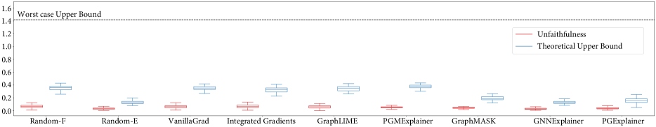
Figure 1: Empirically calculated unfaithfulness (in red) and our theoretical bounds for unfaithfulness (in blue) across nine explanation methods. Results on the German credit graph dataset show no violations of our theoretical bounds. Results for stability, counterfactual fairness mismatch, and group fairness mismatch are shown in Appendix Figs. 2-3.

Table 1: Systematic evaluation of GNN explanation methods (random strategies (in grey), gradient- (in yellow), surrogate- (in purple), and perturbation-based (in red) methods) for node classification. Shown are average values and standard errors of evaluation metrics across all test set nodes. Arrows ($\downarrow$) indicate the direction of better performance. Surrogate-based methods produce most reliable explanations across all datasets. Note that fairness does not apply to some datasets (i.e., N/A) as they do not contain sensitive features. See Table C.1-4 for results on all 9 datasets.

		Evaluation metrics
Dataset	Method	Unfaithfulness ($\downarrow$)	Instability ($\downarrow$)	Fairness Mismatch ($\downarrow$)
				Counterfactual	Group
Credit defaulter graph	Random Node Features Random Edges VanillaGrad Integrated Gradients GraphLIME PGMExplainer GraphMASK GNNExplainer PGExplainer	0.098$\pm$0.002 0.020$\pm$0.001 0.092$\pm$0.002 0.147$\pm$0.003 0.038$\pm$0.002 0.283$\pm$0.002 0.012$\pm$0.001 0.021$\pm$0.001 0.028$\pm$0.001	0.426$\pm$0.002 0.376$\pm$0.000 0.333$\pm$0.002 0.140$\pm$0.002 0.225$\pm$0.004 0.156$\pm$0.002 0.036$\pm$0.002 0.375$\pm$0.000 0.364$\pm$0.001	0.424$\pm$0.002 0.376$\pm$0.000 0.171$\pm$0.002 0.069$\pm$0.001 0.063$\pm$0.003 0.154$\pm$0.002 0.004$\pm$0.000 0.366$\pm$0.000 0.348$\pm$0.002	0.045$\pm$0.002 0.017$\pm$0.001 0.042$\pm$0.002 0.053$\pm$0.002 0.018$\pm$0.001 0.161$\pm$0.003 0.010$\pm$0.001 0.019$\pm$0.001 0.022$\pm$0.001
Ogbn-arxiv	Random Node Features Random Edges VanillaGrad Integrated Gradients GraphLIME PGMExplainer GraphMASK GNNExplainer PGExplainer	0.529$\pm$0.002 0.431$\pm$0.002 0.528$\pm$0.002 0.528$\pm$0.002 0.260$\pm$0.003 0.413$\pm$0.002 0.586$\pm$0.001 0.430$\pm$0.002 0.338$\pm$0.002	0.375$\pm$0.000 0.378$\pm$0.001 0.359$\pm$0.001 0.372$\pm$0.000 0.374$\pm$0.004 0.270$\pm$0.002 0.125$\pm$0.002 0.376$\pm$0.001 0.381$\pm$0.001	N/A        N/A        N/A        N/A        N/A        N/A        N/A        N/A        N/A	N/A        N/A        N/A        N/A        N/A        N/A        N/A        N/A        N/A

Empirically verifying our theoretical bounds. We analytically evaluated our theoretical bounds by computing the LHS of Eqns. 1,2,6,10 for all the nine explanation methods. Fig. 1 shows the empirical and theoretical bounds for the unfaithfulness of methods, empirically confirming that none of our theoretical bounds were violated. Not only are we introducing theoretical bounds (RHS of the Eqns. 1,2,6,10) for a broad range of explanation methods, but our bounds are also tight in the sense that their differences with empirical estimates are an order of magnitude smaller than those provided by the worst-case upper bounds (calculated using the maximum difference between the softmax scores of predictions made using original and masked node features/edges). For instance, the empirical estimate and the theoretical bound for the unfaithfulness of GNNExplainer match very closely (Fig. 1). We also computed the Spearman’s rank correlation between the rankings for each of nine methods based on the theoretical bounds vs. empirical estimates of unfaithfulness. The correlation is $0.72$ (p-value=$0.03$) suggesting a strong correspondence between our theoretical bounds and empirical estimates. Results for stability and fairness preservation are shown in Figs. 2-3 in the Appendix.

Evaluating the reliability of GNN explanation methods. We compare the reliability of explanation methods by computing unfaithfulness (Eqn. 1), instability (Eqn. 2), counterfactual (Eqn. 6) and group fairness mismatch (Eqn. 10) metrics as described above. Results in Table 1,C.1,4 show that surrogate-based explanation methods produce more reliable explanations than gradient- and perturbation-based methods. We observe that while no explanation method simultaneously preserves all properties, on average across all node classification datasets (Fig. C.1), surrogate-based methods outperform other methods in instability (+55.1%) and counterfactual fairness mismatch (+103.7%), whereas perturbation-based methods outperform other methods in unfaithfulness (+23.8%) and group fairness mismatch (+116.7%). Interestingly, we find that the Random Edge baselines, which output explanations that correspond to random sets of edges incident on the target node, achieves the lowest (best possible) unfaithfulness score on most datasets, highlighting the urgent need for further probing of the behavior of all the GNN explainers. Finally, across all datasets (Fig. 4), explanations based on graph structure are slightly more faithful (+11.6%), stable (+6.2%), and counterfactually fair (+3.1%).

Analyzing the trade-offs between faithfulness, stability, and fairness mismatch. We explore the trade-offs and possible connections between different properties defined in Sec. 3. Results in Table 1,C.1,4 (e.g., GNNExplainer on Recidivism and Credit defaulter graphs) indicate that methods with lower values of unfaithfulness (Eqn. 1) also exhibit lower values of group fairness (Eqn. 10) mismatch (and vice versa). To verify this connection, we compute the Pearson’s and Spearman’s rank correlation on the unfaithfulness and group fairness mismatch values and observe a strong positive correlation between them (Pearson’s $r$=0.87 with p-value=4.82e-09; Spearman’s $\rho$=0.87 with p-value=2.67e-09). We also observe a connection between instability (Eqn. 2) and counterfactual fairness mismatch (Eqn. 6) metrics, where methods with lower values of instability (e.g., GraphMASK on Credit defaulter graph) also exhibit lower values of counterfactual fairness mismatch (and vice versa). We further observe a strong positive correlation between instability and counterfactual fairness mismatch (Pearson’s $r$=0.85 with p-value=2.72e-08; Spearman’s $\rho$=0.86 with p-value=6.13e-09).

Other downstream tasks. We also apply our framework to link prediction and graph classification. We extend some existing methods for these tasks as most GNN explanation methods were developed only for node classification. Explanations for these tasks also consist of a node feature mask and/or edge mask. We generate these node feature/edge masks as described in Sec. 3 and evaluate all the properties. Similar to node classification, we observe that random baselines perform at least on par or better than the state-of-the-art GNN explanation methods (Table 5).

5 CONCLUSIONS

We introduce the first-ever theoretical analysis of the reliability of GNN explanation methods. To this end, we analyze the behavior of nine diverse state-of-the-art GNN explanation methods through the lens of various desirable properties such as faithfulness, stability, and fairness preservation. Specifically, we establish theoretical upper bounds on the violation of each of these properties. Our theoretical analyses rely on information and probability theory concepts including data processing inequalities and total variation distance, and Lipschitz continuity. Further, we carry out extensive empirical analysis with nine real world datasets to verify our theoretical guarantees, and examine trade-offs between faithfulness, stability, and fairness preservation properties. These results yield critical insights on the behavior of state-of-the-art GNN explanation methods which can in turn inform the design and development of future explanation methods.

Acknowledgements

We would like to thank the anonymous reviewers for their insightful feedback. M.Z. is supported, in part by NSF under nos. IIS-2030459 and IIS-2033384, Harvard Data Science Initiative, Amazon Research Award, Bayer Early Excellence in Science Award, AstraZeneca Research, Roche Alliance with Distinguished Scientists (ROADS) Award, Department of the Air Force, and MIT Lincoln National Laboratory. H.L. is supported, in part by the NSF awards IIS-2008461 and IIS-2040989, and research awards from the Harvard Data Science Institute, Amazon, Bayer, and Google. H.L. would like to thank Mohan and Sujatha Lakkaraju, and Pracheer Gupta for all their inputs and support. The views expressed are those of the authors and do not reflect the official policy or position of the funding agencies.

 

Supplementary Materials: Probing GNN Explainers: Rigorous Theoretical and Empirical Analysis of GNN Explanation Methods

 

Appendix A Overview of GNN Explanation Methods

We now provide an in-depth overview of the different GNN explanation methods that we analyze in this work. As described in the main text (Sec. 3), a $\mathcal{G}{=}(\mathcal{V},\mathcal{E},\mathbf{X})$ denote an undirected and unweighted graph comprising of a set of nodes $\mathcal{V}$, a set of edges $\mathcal{E}$, and a set of node feature vectors $\mathbf{X}{=}\{\mathbf{x}_{1},\dots,\mathbf{x}_{N}\}$ corresponding to nodes in $\mathcal{V}$, where $\mathbf{x}_{u}{\in}\mathbb{R}^{M}$. The GNN model’s $f$ softmax prediction for node $u$ is given by $\mathbf{\hat{y}}_{u}=f(\mathcal{G}_{u})$, where $\mathcal{G}_{u}$ denotes the subgraph associated with node $u$ and $\mathbf{\hat{y}}_{u}\in[0,1]^{C}$. Finally, the explanation $E_{u}$ consists of a discrete node feature mask $\mathbf{r}_{u}\in\{0,1\}^{M}$ for $v\in\mathcal{N}_{u}$ and/or a discrete edge mask $\mathbf{R}_{u}\in\{0,1\}^{N\times N}$, where $1$ indicates that a node attribute/edge is included in the explanation and $0$ indicates otherwise.

Random Explanations. As a control, we consider two methods which produce random explanations: 1) Random Node Features–a node feature mask defined by an $M$-dimensional Gaussian distributed vector; and 2) Random Edges–an $N\times N$ edge mask drawn from a uniform distribution over $u$’s incident edges.

VanillaGrad. Gradient (Simonyan et al., 2014) based explanation generate local explanations for the prediction of a differentiable GNN model $f$ using its gradient with respect to the node features $\mathbf{x}_{u}$: $\triangledown_{\mathbf{x}_{u}}f$. Intuitively, gradient represents how much difference a tiny change in each feature of a node $u$ would make to its corresponding classification score. VanillaGrad output an $M$-dimensional vector that comprises the vanilla gradient of the model, as explanations.

Integrated Gradients. Gradient explanations are often noisy and suffer from saturation problems (Sundararajan et al., 2017). Integrated gradients addresses the gradient saturation problem by averaging the gradients over a set of interpolated inputs derived using node $u$’s attribute and a baseline. Formally, integrated gradient explanation for a node $u$ is an $M$-dimensional vector given by:

$$E_{u}=(\mathbf{x}_{u}-\mathbf{\tilde{x}})\times\int_{\alpha=0}^{1}\frac{\partial{f(\mathcal{G}_{u^{\prime}})}}{\partial{\mathbf{x}_{u}}}d\alpha,$$ (11)

where $\mathbf{\tilde{x}}$ is the baseline input which can be vector of all zeros/ones and $\mathcal{G}_{u^{\prime}}$ denotes the graph with the interpolated node attribute $\mathbf{x}_{u^{\prime}}{=}\mathbf{\tilde{x}}{+}\alpha(\mathbf{x}_{u}{-}\mathbf{\tilde{x}})$.

GraphLIME. GraphLIME (Huang et al., 2020) is a local interpretable model explanation for GNNs that identifies a nonlinear interpretable model over the neighbors of a node that is locally faithful to the node’s prediction. It considers a feature-wise kernelized nonlinear method called Hilbert-Schmidt Independence Criterion Lasso (HSIC Lasso) as an explanation model. For each node prediction, the HSIC Lasso objective function is defined as:

$$\min_{\beta\in\mathbb{R}^{d}}\frac{1}{2}||\mathbf{L}-\sum_{k=1}^{M}\beta_{k}\mathbf{K}^{(k)}||^{2}_{F}+\rho||\beta||_{1},$$ (12)

where $||\cdot||_{F}$ is the Frobenius norm, $\rho\geq 0$ is the regularization parameter, $||\cdot||_{1}$ is the $l_{1}$ norm to enforce sparsity, $\mathbf{L}$ is the centered Gram matrix, $L_{ij}=L(y_{i},y_{j})$ is the kernel for the output labels of the nodes, $\mathbf{K}^{k}$ is the centered gram matrix for the $k$-th feature, and $K_{ij}=K(x_{i}^{(k)},x_{j}^{(k)})$ is the kernel for the $k$-th dimensional input node features $\mathbf{x}_{u}$.

PGMExplainer. Probabilistic Graphical models (PGMs) are statistical models that encode complex distributions using graph-based representation and provides a simple interpretation of the dependencies of those underlying random variables. Specifically, Bayesian network, a PGM represents conditional dependencies among variables via a directed acyclic graph. Given a target prediction $\hat{y}_{u}$ to be explained, our proposed PGM explanation is the optimal Bayesian network $\mathcal{B}^{*}$ of the following optimization:

$$\operatorname*{arg\,max}_{\mathcal{B}\in\mathcal{B}_{E_{u}}}R_{\hat{y}_{u}}(\mathcal{B}),$$ (13)

where $R_{\hat{y}_{u}}:E_{u}\to\mathbb{R}$ associates each explanation with a score, $\mathcal{B}_{E_{u}}$ is the set of all Bayesian networks, the optimization is subjected to the condition that the number of variables in $\mathcal{B}$ is bounded by a constant to encourage a compact solution and another constraint to ensure that the target prediction is included in the explanation.

GraphMASK. GraphMASK (Schlichtkrull et al., 2021) detect edges at each layer $l$ that can be ignored without affecting the output model predictions. In general, dropping edges from a given graph is non-trivial, and, hence, for each edge at layer $l$, GraphMASK learns a binary choice $z^{l}_{u,v}$ that indicates whether the edge can be dropped, and then replaces the given edge with a learned baseline. Here, $z^{l}_{u,v}$ indicates an edge connecting node $u$ and $v$. GraphMASK learns $z^{l}_{u,v}$ for all $(u,v)\in\mathcal{E}$ for the training data points using an erasure function $g_{\pi}$, where $\pi$ denotes the parameters of $g$. For explaining a given prediction, GraphMASK uses this trained function $g_{\pi}$ and generates a masked representation of the graph using:

$$\tilde{h}_{u}^{l}{=}\mathbf{Z}^{l}\circ h_{u}^{l}+\alpha^{l}\circ(1-\mathbf{Z}^{l}),$$ (14)

where $\mathbf{Z}^{l}$ comprises of all the individual binary scores $z^{l}_{u,v}=g_{\pi}(h_{u}^{l},h_{v}^{l})$, $\alpha^{l}$ is the learned baseline, and ‘$\circ$’ denotes the element-wise Hadamard product.

GNNExplainer. For a single-instance explanation for node $u$, GNNExplainer (Ying et al., 2019) generates an explanation by identifying a subgraph of the computation graph for $u$ and a subset of node features that are most influential for the model $f$’s prediction. Formally, GNNExplainer determines the importance of individual node attributes and incident edges for node $u$ by leveraging Mutual Information ($MI$) using the following optimization framework:

$$\max_{\mathcal{G}_{S}}MI(Y,(\mathcal{G}_{S},\mathbf{X}_{S})),$$ (15)

where $\mathcal{G}_{S}\subseteq\mathcal{G}_{u}$ is a subgraph and $\mathbf{X}_{S}$ is the associated node attributes that are important for the GNN’s prediction $\hat{y}_{u}$. Intuitively, $MI$ quantifies the change in probability of prediction $\hat{y}_{u}$ when $u$’s computation graph is limited to the explanation graph $\mathcal{G}_{S}$ and its corresponding node attributes $\mathbf{X}_{S}$.

PGExplainer. In contrast to GNNExplainer, PGExplainer (Luo et al., 2020) generates explanation only on the graph structure. The direct optimization of the mutual information framework in Eqn. 15 is intractable (Ying et al., 2019; Luo et al., 2020). Thus, PGExplainer consider a relaxation by assuming that the explanatory graph $\mathcal{G}_{S}$ is a Gilbert random graph, where selections of edges from the input graph $\mathcal{G}_{u}$ are conditionally independent to each other. Due to the discrete nature of $\mathcal{G}_{S}$, PGExplainer employs the reparameterization trick where they relax the edge weights from binary to continuous variables in the range $(0,1)$ and then optimize the objective function using gradient-based methods. It approximates the sampling process of $\mathcal{G}_{S}$ with a determinant function of parameters $\Omega$, temperature $\rho$, and an independent random variable $\epsilon$. Specifically, the weight for each edge $\hat{e}(i,j)$ is calculated by:

$$\epsilon\sim\text{Uniform}(0,1),\leavevmode\nobreak\ \leavevmode\nobreak\ \hat{e}(i,j)=\sigma((\text{log}\epsilon-\text{log}(1-\epsilon)+\omega_{ij})/\rho),$$ (16)

where $\sigma(\cdot)$ is the Sigmoid function, $\omega_{ij}\in\mathbb{R}$ is a trainable parameter. With the reparameterization, the objective function of PGExplainer becomes:

$$\min_{\Omega}\mathbb{E}_{\epsilon\sim\text{Uniform}(0,1)}\leavevmode\nobreak\ H(Y|\mathcal{G}_{u}=\mathcal{\hat{G}}_{S}),$$ (17)

where $H$ is the conditional entropy when the computational graph for $\mathcal{G}_{u}$ is restricted to $\mathcal{G}_{S}$.

Note that recently proposed explanation methods, such as GNN-LRP (Schnake et al., 2020), Xgnn (Yuan et al., 2020a), and Gem (Lin et al., 2021), can also be empirically analyzed using our framework because all these methods generate explanations using subgraphs around the target node with associated edges and node attributes. Hence, we can select the topk edges/nodes from the subgraph and calculate the metric scores.

Appendix B Proofs for Theorems in Section 3

B.1 Analyzing Faithfulness of GNN Explanation Methods

Theorem 1. Given a node $u$ and a set $\mathcal{K}$ of node perturbations, the unfaithfulness (Sec. 3.1, Eqn. 1) of its explanation $E_{u}$ can be bounded as follows:

$$\frac{1}{|\mathcal{K}|}\sum_{u^{\prime}\in\mathcal{K}}||f(\mathcal{G}_{u^{\prime}})-f(t(E_{u},\mathcal{G}_{u^{\prime}}))||_{2}\leq\gamma\leavevmode\nobreak\ \frac{(1{+}|\mathcal{K}|)}{|\mathcal{K}|}\leavevmode\nobreak\ ||\Delta||_{2},$$

where $f(\mathcal{G}_{u^{\prime}})=\mathbf{\hat{y}}_{u^{\prime}}$ are softmax predictions that use original attributes and $f(t(E_{u},\mathcal{G}_{u^{\prime}}))=\mathbf{\hat{y}}_{u^{\prime}}^{E}$ are softmax predictions that use attributes marked important by explanation $E_{u}$. Further, $\gamma$ denotes the product of the Lipschitz constants for GNN’s activation function and GNN’s weight matrices across all layers in the GNN, and $\Delta$ is an explanation method-specific term.

Proof.  Without loss of generality, we use a two-layer GNN model for our proof and show its extension to a GNN model with $L$ layers. The two-layer GNN formulated as a message-passing network is defined as:

$$\mathbf{h}_{u}^{1}{=}\text{sp}(\mathbf{W}_{a}^{1}\mathbf{x}_{u}+\mathbf{W}_{n}^{1}\sum_{v\in\mathcal{N}_{u}}\mathbf{x}_{v})$$

$$\mathbf{h}_{u}^{2}{=}\mathbf{W}_{\text{fc}}\mathbf{h}_{u}^{1}+\mathbf{b}$$

$$\mathbf{\hat{y}}_{u}{=}\text{softmax}(\mathbf{h}_{u}^{2}),$$

where $\mathbf{W}_{n}^{1}$ is the weight matrix associated with the neighbors of node $u$, $\mathbf{W}_{a}^{1}$ is the self-attention weight matrix at layer one, and “sp” is the softplus activation function. For the fully-connected layer, we have $\mathbf{W}_{\text{fc}}$ as the weight matrix and $\mathbf{b}$ as the bias term. The softplus function is a smooth approximation of the ReLU function. We generate $|\mathcal{K}|$ perturbations of node $u$ by adding normal Gaussian noise to the node features, i.e., $\mathbf{x}_{u^{\prime}}{=}\mathbf{x}_{u}{+}\tau$, and rewire edges with some probability $p_{r}$. For faithfulness, we get the predictions for node $u$ using the weighted node features of node $u$, i.e., the element-wise product between $\mathbf{r}_{u}$ (the feature importance mask generated as an explanation) and $\mathbf{x}_{u}$. Let $\mathbf{\hat{y}}_{u}^{E}$ denote the softmax output for node $u$ using the explanation $E_{u}$, i.e., $f(t(E_{u},\mathcal{G}_{u}))$. Therefore, the updated equations using the explanations are:

$$(\mathbf{h}_{u}^{1})^{E}=\text{sp}\big{(}\mathbf{W}_{a}^{1}(\mathbf{r}_{u}\circ\mathbf{x}_{u})+\mathbf{W}_{n}^{1}\sum_{v\in\mathcal{N}^{\prime}_{u}}\mathbf{x}_{v}\big{)}$$

$$(\mathbf{h}_{u}^{2})^{E}=\mathbf{W}_{\text{fc}}(\mathbf{h}_{u}^{1})^{E}+\mathbf{b}$$

$$\mathbf{\hat{y}}_{u}^{E}=\text{softmax}((\mathbf{h}_{u}^{2})^{E}),$$

where $\mathcal{N}^{\prime}_{u}$ denotes the new neighborhood for node $u$ due to the adjacency mask matrix $\mathbf{R}_{u}$. The difference between the predicted labels for the original and the important node features can be given as:

$$\mathbf{\hat{y}}_{u}-\mathbf{\hat{y}}_{u}^{E}=\text{softmax}(\mathbf{h}_{u}^{2})-\text{softmax}((\mathbf{h}_{u}^{2})^{E})$$ (18)

Corollary 1. For any differentiable function $g:\mathbb{R}^{a}\to\mathbb{R}^{b}$,

$$||g(x)-g(y)||_{2}\leq||\mathbf{J}||^{*}_{F}||x-y||_{2}\leavevmode\nobreak\ \leavevmode\nobreak\ \leavevmode\nobreak\ \leavevmode\nobreak\ \forall x,y\in\mathbb{R},$$ (19)

where $||\mathbf{J}||^{*}_{F}=\max_{x}||\mathbf{J}||_{F}$ and $\mathbf{J}$ is the Jacobian matrix of $g(x)$ w.r.t. $x$. This is implied from the mean value theorem, where for any function $g(x)$ and its derivative $\frac{\partial{g(x)}}{\partial{x}}$, we have: $g(x)-g(y)=\frac{\partial{g(\phi)}}{\partial{\phi}}(x-y)$, for some $\phi\in(y,x)$.

Hence, taking the norm on both sides in Eqn. 18, we get,

$$||\mathbf{\hat{y}}_{u}-\mathbf{\hat{y}}_{u}^{E}||_{2}=||\text{softmax}(\mathbf{h}_{u}^{2})-\text{softmax}((\mathbf{h}_{u}^{2})^{E})||_{2}$$

$$\leq\mathcal{C}_{\text{fc}}||\mathbf{h}_{u}^{2}-(\mathbf{h}_{u}^{2})^{E}||_{2},$$ (Using Corollary 1)

where $\mathcal{C}_{\text{fc}}$ represents the Lipschitz constant for the softmax function. Substituting the values of $\mathbf{h}_{u}^{2}$ and $(\mathbf{h}_{u}^{2})^{E}$ we get:

$$||\mathbf{\hat{y}}_{u}-\mathbf{\hat{y}}_{u}^{E}||_{2}\leq\mathcal{C}_{\text{fc}}||\mathbf{W}_{\text{fc}}\mathbf{h}_{u}^{1}+\mathbf{b}-\mathbf{W}_{\text{fc}}(\mathbf{h}_{u}^{1})^{E}-\mathbf{b}||_{2}$$

$$\leq\mathcal{C}_{\text{fc}}||\mathbf{W}_{\text{fc}}\mathbf{h}_{u}^{1}-\mathbf{W}_{\text{fc}}(\mathbf{h}_{u}^{1})^{E}||_{2}$$

$$\leq\mathcal{C}_{\text{fc}}\leavevmode\nobreak\ ||\mathbf{W}_{\text{fc}}||_{2}\leavevmode\nobreak\ ||\mathbf{h}_{u}^{1}-(\mathbf{h}_{u}^{1})^{E}||_{2}$$ (Using Cauchy-Schwartz inequality)

Substituting the values of $\mathbf{h}_{u}^{1}$ and $(\mathbf{h}_{u}^{1})^{E}$ we get:

$$||\mathbf{\hat{y}}_{u}-\mathbf{\hat{y}}_{u}^{E}||_{2}\leq\mathcal{C}_{\text{fc}}\leavevmode\nobreak\ ||\mathbf{W}_{\text{fc}}||_{2}\leavevmode\nobreak\ ||\text{sp}\big{(}\mathbf{W}_{a}^{1}\mathbf{x}_{u}+\mathbf{W}_{n}^{1}\sum_{v\in\mathcal{N}_{u}}\mathbf{x}_{v}\big{)}-\text{sp}\big{(}\mathbf{W}_{a}^{1}(\mathbf{r}_{u}\circ\mathbf{x}_{u})+\mathbf{W}_{n}^{1}\sum_{v\in\mathcal{N}^{\prime}_{u}}\mathbf{x}_{v}\big{)}||_{2}$$

$$\leq\mathcal{C}_{\text{fc}}\leavevmode\nobreak\ \mathcal{C}_{1}\leavevmode\nobreak\ ||\mathbf{W}_{\text{fc}}||_{2}\leavevmode\nobreak\ ||\mathbf{W}_{a}^{1}\mathbf{x}_{u}+\mathbf{W}_{n}^{1}\sum_{v\in\mathcal{N}_{u}}\mathbf{x}_{v}-\mathbf{W}_{a}^{1}(\mathbf{r}_{u}\circ\mathbf{x}_{u})-\mathbf{W}_{n}^{1}\sum_{v\in\mathcal{N}^{\prime}_{u}}\mathbf{x}_{v}||_{2}$$ (Using Corollary 1)

$$\leq\mathcal{C}_{\text{fc}}\leavevmode\nobreak\ \mathcal{C}_{1}\leavevmode\nobreak\ ||\mathbf{W}_{\text{fc}}||_{2}\leavevmode\nobreak\ \big{(}||\mathbf{W}_{a}^{1}\big{(}\mathbf{x}_{u}-(\mathbf{r}_{u}\circ\mathbf{x}_{u})\big{)}||_{2}+||\mathbf{W}_{n}^{1}\Delta_{\mathbf{x}_{v}}||_{2}\big{)},$$ (Using triangle inequality)

where $\Delta_{\mathbf{x}_{v}}$ is the difference between the representations of the neighbors of $u$ after dropping edges using the edge masks. This difference can be neglected for gradient and GraphLIME methods as they provide explanations in the node feature space. Now, using Cauchy-Schwartz inequality, the prediction difference for a node $u$ using its original and just important node features is bounded by:

$$||\mathbf{\hat{y}}_{u}-\mathbf{\hat{y}}_{u}^{E}||_{2}\leq\mathcal{C}_{\text{fc}}\leavevmode\nobreak\ \mathcal{C}_{1}\leavevmode\nobreak\ ||\mathbf{W}_{\text{fc}}||_{2}\leavevmode\nobreak\ ||\mathbf{W}_{a}^{1}||_{2}\leavevmode\nobreak\ ||(\mathbf{1}-\mathbf{r}_{u})\circ\mathbf{x}_{u})||_{2},$$ (20)

where $\mathcal{C}_{1}$ is the Lipschitz constant for the softplus activation function and $\mathbf{1}\in\mathbb{R}^{M}$ is vector with all ones. For mathematical brevity, let $\gamma_{11}=\mathcal{C}_{\text{fc}}\leavevmode\nobreak\ \mathcal{C}_{1}\leavevmode\nobreak\ ||\mathbf{W}_{\text{fc}}||_{2}\leavevmode\nobreak\ ||\mathbf{W}_{a}^{1}||_{2}$. Similarly, the prediction difference for GraphMASK which provides an explanation with respect to edges is bounded by:

$$||\mathbf{\hat{y}}_{u}-\mathbf{\hat{y}}_{u}^{E}||_{2}\leq\mathcal{C}_{\text{fc}}\leavevmode\nobreak\ \mathcal{C}_{1}\leavevmode\nobreak\ ||\mathbf{W}_{\text{fc}}||_{2}\leavevmode\nobreak\ ||\mathbf{W}_{n}^{1}||_{2}\leavevmode\nobreak\ ||\Delta_{\mathbf{x}_{v}}||_{2},$$ (21)

where $\gamma_{12}=\mathcal{C}_{\text{fc}}\leavevmode\nobreak\ \mathcal{C}_{1}\leavevmode\nobreak\ ||\mathbf{W}_{\text{fc}}||_{2}\leavevmode\nobreak\ ||\mathbf{W}_{n}^{1}||_{2}$.

Node feature explanations. Since all the perturbed nodes use the same node feature explanation $\mathbf{r}_{u}$, we obtain the difference between the predictions for a perturbed node $u^{\prime}$ using the perturbed and the masked node features, i.e.,

$$||\mathbf{\hat{y}}_{u^{\prime}}-\mathbf{\hat{y}}_{u^{\prime}}^{E}||_{2}\leq\gamma_{11}\leavevmode\nobreak\ ||\mathbf{x}_{u^{\prime}}-(\mathbf{r}_{u}\circ\mathbf{x}_{u^{\prime}})||_{2},$$

where $\mathbf{\hat{y}}_{u^{\prime}}$ is the softmax prediction using the perturbed node feature $\mathbf{x}_{u^{\prime}}=\mathbf{x}_{u}+\tau$, and as per the definition of faithfulness we use the explanation mask of node $u$ for node $u^{\prime}$. Finally, we get:

$$||\mathbf{\hat{y}}_{u^{\prime}}-\mathbf{\hat{y}}_{u^{\prime}}^{E}||_{2}\leq\gamma_{11}\leavevmode\nobreak\ ||(\mathbf{1}-\mathbf{r}_{u})\circ\mathbf{x}_{u^{\prime}}||_{2}$$ (22)

For faithfulness, we generate a set of $\mathcal{K}$ perturbed nodes and get $|\mathcal{K}|$ predictions from the model for each of the corresponding perturbations. Using Eqns. 20 and 22, and getting the predictions from all $|\mathcal{K}|$ perturbations, we get:

$$\sum_{u^{\prime}\in\mathcal{K}}||\mathbf{\hat{y}}_{u^{\prime}}-\mathbf{\hat{y}}_{u^{\prime}}^{E}||_{2}\leq\gamma_{11}\leavevmode\nobreak\ ||(\mathbf{1}-\mathbf{r}_{u})\circ\mathbf{x}_{u})||_{2}+\gamma_{11}\sum_{u^{\prime}\in\mathcal{K}}\leavevmode\nobreak\ ||(\mathbf{1}-\mathbf{r}_{u})\circ\mathbf{x}_{u^{\prime}}||_{2}$$

$$\leq\gamma_{11}\leavevmode\nobreak\ ||(\mathbf{1}-\mathbf{r}_{u})\circ\mathbf{x}_{u})||_{2}+\gamma_{11}\leavevmode\nobreak\ ||(\mathbf{1}-\mathbf{r}_{u})\circ\sum_{u^{\prime}\in\mathcal{K}}\mathbf{x}_{u^{\prime}}||_{2},$$

Assuming $\tau$ to be drawn from a normal distribution, we get: $\sum_{u^{\prime}\in\mathcal{K}}\mathbf{x}_{u^{\prime}}=|\mathcal{K}|\mathbf{x}_{u}+\sum_{u^{\prime}\in\mathcal{K}}\tau_{k}$. For sufficiently large $|\mathcal{K}|$, we have: $\sum_{u^{\prime}\in\mathcal{K}}(\mathbf{x}_{u}^{{}^{\prime}})_{k}\approx|\mathcal{K}|\mathbf{x}_{u}$. Putting everything together and taking the average across $\mathcal{K}$ samples we get,

$$\frac{1}{\mathcal{|K|}}\sum_{u^{\prime}\in\mathcal{K}}||\mathbf{\hat{y}}_{u^{\prime}}-\mathbf{\hat{y}}_{u^{\prime}}^{E}||_{2}\leq\frac{1}{\mathcal{|K|}}\big{(}\gamma_{11}\leavevmode\nobreak\ ||(\mathbf{1}-\mathbf{r}_{u})\circ\mathbf{x}_{u})||_{2}+\gamma_{11}\leavevmode\nobreak\ |\mathcal{K}|\leavevmode\nobreak\ ||(\mathbf{1}-\mathbf{r}_{u})\circ\mathbf{x}_{u}||_{2}\big{)}$$

$$\leq\gamma_{11}\leavevmode\nobreak\ \frac{(1{+}|\mathcal{K}|)}{\mathcal{|K|}}\leavevmode\nobreak\ ||(\mathbf{1}-\mathbf{r}_{u})\circ\mathbf{x}_{u}||_{2}$$

For a GNN model with $L$ message-passing layers and one fully-connected layer for node classification, $\gamma_{11}$ takes the general form of:

$$\gamma_{11}=\mathcal{C}_{\text{fc}}\leavevmode\nobreak\ ||\mathbf{W}_{\text{fc}}||_{2}\leavevmode\nobreak\ \prod_{l=1}^{L}\mathcal{C}_{l}||\mathbf{W}_{a}^{l}||_{2},$$ (23)

where $\mathcal{C}_{\text{fc}}$ is the Lipschitz constant for the softmax activation operating on the fully-connected layer, $\mathbf{W}_{\text{fc}}$ is the weight matrix associated with the fully-connected layer, $\mathcal{C}_{l}$ is the Lipschitz constant of the softplus activation of each message-passing layer, and $\mathbf{W}_{a}^{l}$ is the self-attention weight associated with the $l$-th message-passing layer.

Edge explanations. Note, the difference between the predictions for a perturbed node $u^{\prime}$ using the perturbed and the masked node features will be similar to Eqn. B.1 as for faithfulness, the perturbations are made only in node $u$, i.e.,

$$||\mathbf{\hat{y}}_{u^{\prime}}-\mathbf{\hat{y}}_{u^{\prime}}^{E}||_{2}\leq\gamma_{12}\leavevmode\nobreak\ ||\Delta_{\mathbf{x}_{v}}||_{2},$$

Also, since we use the same explanation for all the nodes in set $\mathcal{K}$, the bound for faithfulness using edge explanations is given by:

$$\frac{1}{\mathcal{|K|}}\sum_{u^{\prime}\in\mathcal{K}}||\mathbf{\hat{y}}_{u^{\prime}}-\mathbf{\hat{y}}_{u^{\prime}}^{E}||_{2}\leq\gamma_{12}\leavevmode\nobreak\ \frac{(1{+}|\mathcal{K}|)}{|\mathcal{K}|}\leavevmode\nobreak\ ||\Delta_{\mathbf{x}_{v}}||_{2},$$

where as in Eqn. 23, $\gamma_{12}$ can take the general form for $L$ message-passing layers as: $\gamma_{12}=\mathcal{C}_{\text{fc}}\leavevmode\nobreak\ ||\mathbf{W}_{\text{fc}}||_{2}\leavevmode\nobreak\ \prod_{l=1}^{L}\mathcal{C}_{l}||\mathbf{W}_{n}^{l}||_{2}$.

B.2 Analyzing Stability of GNN Explanation Methods

B.2.1 VanillaGrad Explanation

Theorem 2. Given a non-linear activation function $\sigma$ that is Lipschitz continuous, the instability (Sec. 3.2, Eqn. 2) of explanation $E_{u}$ returned by VanillaGrad method can be bounded as follows:

$$||\triangledown_{\mathbf{x}_{u^{\prime}}}f-\triangledown_{\mathbf{x}_{u}}f||_{p}\leq\gamma_{3}||\mathbf{x}_{u^{\prime}}-\mathbf{x}_{u}||_{p},$$ (24)

where $\gamma_{3}$ is a constant, $\mathbf{x}_{u}$ is node $u$’s feature vector, and $\mathbf{x}_{u^{\prime}}$ is the perturbed node feature vector.

Proof.  Similar to Sec. B.1, let us consider a two-layer GNN model trained on a node classification task using softmax cross-entropy loss function with the first layer a message-passing GNN layer and the second layer as a fully-connected layer. The cross-entropy (CE) loss is given as:

$$\text{CE}=-\sum_{i}y_{i}\log\hat{y}_{u},$$ (25)

where $\mathbf{y}$ is a vector with one one non-zero element (which is 1), $\mathbf{\hat{y}}_{u}{=}\text{softmax}(\mathbf{h}_{u}^{2})$, $\mathbf{h}_{u}^{2}{=}\mathbf{W}_{\text{fc}}\mathbf{h}_{u}^{1}+\mathbf{b}$, and $\mathbf{h}_{u}^{1}{=}\text{sp}(\mathbf{W}_{a}^{1}\mathbf{x}_{u}+\mathbf{W}_{n}^{1}\sum_{v\in\mathcal{N}_{u}}\mathbf{x}_{v})$. $\mathbf{W}_{n}^{1}$ is the weight matrix associated with the neighbors of node $u$ and $\mathbf{W}_{a}^{1}$ is the self-attention weight matrix at layer one. For the fully-connected layer, we have $\mathbf{W}_{\text{fc}}$ as the weight matrix and $\mathbf{b}$ as the bias term. “sp” is the softplus activation function which is a smooth approximation of the ReLU function. For stability, we generate $\mathbf{x}_{u^{\prime}}$ by adding noise to the node features of node $u$ and keep everything else constant. Therefore, $\mathbf{h}_{u^{\prime}}^{1}=\text{sp}(\mathbf{W}_{a}^{1}\mathbf{x}_{u^{\prime}}+\mathbf{W}_{n}^{1}\sum_{v\in\mathcal{N}^{\prime}_{u}}\mathbf{x}_{v})$. Now, the differentiation of the model w.r.t. the node features can be given as:

$$\triangledown_{\mathbf{x}_{u}}f=\frac{\partial{(\text{CE})}}{\partial{\mathbf{x}_{u}}}=\frac{\partial{(\text{CE})}}{\partial{\mathbf{h}_{u}^{2}}}\frac{\partial{\mathbf{h}_{u}^{2}}}{\partial{\mathbf{h}_{u}^{1}}}\frac{\partial{\mathbf{h}_{u}^{1}}}{\partial{\mathbf{x}_{u}}},$$ (By chain rule)

Note, the advantage of using softplus activation function is that it is differentiable for all $x$, i.e.,

$$\text{sp}(x)=\textit{ln}(1+\exp^{x})$$

$$\frac{\partial{(\text{sp}(x))}}{\partial{\text{x}}}=\frac{\exp^{x}}{1+\exp^{x}}\cdot\frac{(1/\exp^{x})}{(1/\exp^{x})}$$

$$=\frac{1}{1+\exp^{-x}}$$

$$=\sigma(x),$$

where $\sigma(\cdot)$ is the sigmoid activation function. Putting it all together we get,

$$\triangledown_{\mathbf{x}_{u}}f=(\mathbf{y}_{u}-\mathbf{\hat{y}}_{u})(\mathbf{W}_{\text{fc}})^{T}\sigma(\mathbf{W}_{a}^{1}\mathbf{x}_{u}+\mathbf{W}_{n}^{1}\sum_{v\in\mathcal{N}_{u}}\mathbf{x}_{v})(\mathbf{W}_{a}^{1})^{T}$$ (26)

$$\triangledown_{\mathbf{x}_{u^{\prime}}}f=(\mathbf{y}_{u}-\mathbf{\hat{y}}_{u})(\mathbf{W}_{\text{fc}})^{T}\sigma(\mathbf{W}_{a}^{1}\mathbf{x}_{u^{\prime}}+\mathbf{W}_{n}^{1}\sum_{v\in\mathcal{N}^{\prime}_{u}}\mathbf{x}_{v})(\mathbf{W}_{a}^{1})^{T}$$ (27)

Note, $\mathbf{\hat{y}}_{u}$ is same for both original and perturbed node according to the Definition 2 in Sec. 3 and we drop the second neighborhood term since the probability ($p_{r}$) of rewiring the edges is very small to maintain the original graph structure. Hence, subtracting the explanations (model gradients) for the original and perturbed node features and taking the norm on both sides, we get:

$$||\triangledown_{\mathbf{x}_{u^{\prime}}}f-\triangledown_{\mathbf{x}_{u}}f||_{p}=||(\mathbf{y}_{u}-\mathbf{\hat{y}}_{u})(\mathbf{W}_{\text{fc}})^{T}\big{(}\sigma(\mathbf{W}_{a}^{1}\mathbf{x}_{u^{\prime}})-\sigma(\mathbf{W}_{a}^{1}\mathbf{x}_{u})\big{)}(\mathbf{W}_{a}^{1})^{T}||_{p},$$

Using Cauchy-Schwartz inequality, we get:

$$||\triangledown_{\mathbf{x}_{u^{\prime}}}f-\triangledown_{\mathbf{x}_{u}}f||_{p}\leq||\mathbf{y}_{u}-\mathbf{\hat{y}}_{u}||_{p}\leavevmode\nobreak\ ||(\mathbf{W}_{\text{fc}})^{T}||_{p}\leavevmode\nobreak\ ||\sigma(\mathbf{W}_{a}^{1}\mathbf{x}_{u^{\prime}})-\sigma(\mathbf{W}_{a}^{1}\mathbf{x}_{u})||_{p}\leavevmode\nobreak\ ||(\mathbf{W}_{a}^{1})^{T}||_{p}$$

Assuming that $\sigma(\cdot)$ is normalized Lipschitz, i.e., $||\sigma{(b)}-\sigma{(a)}||_{p}\leq||b-a||_{p}$, we get,

$$||\triangledown_{\mathbf{x}_{u^{\prime}}}f-\triangledown_{\mathbf{x}_{u}}f||_{p}\leq||\mathbf{y}_{u}-\mathbf{\hat{y}}_{u}||_{p}\leavevmode\nobreak\ ||(\mathbf{W}_{\text{fc}})^{T}||_{p}\leavevmode\nobreak\ ||\mathbf{W}_{a}^{1}\mathbf{x}_{u^{\prime}}-\mathbf{W}_{a}^{1}\mathbf{x}_{u}||_{p}\leavevmode\nobreak\ ||(\mathbf{W}_{a}^{1})^{T}||_{p}$$

$$\leq||\mathbf{y}_{u}-\mathbf{\hat{y}}_{u}||_{p}\leavevmode\nobreak\ ||(\mathbf{W}_{\text{fc}})^{T}||_{p}\leavevmode\nobreak\ ||\mathbf{W}_{a}^{1}(\mathbf{x}_{u^{\prime}}-\mathbf{x}_{u})||_{p}\leavevmode\nobreak\ ||(\mathbf{W}_{a}^{1})^{T}||_{p}$$

$$\leq||\mathbf{y}_{u}-\mathbf{\hat{y}}_{u}||_{p}\leavevmode\nobreak\ ||(\mathbf{W}_{\text{fc}})^{T}||_{p}\leavevmode\nobreak\ ||\mathbf{W}_{a}^{1}||_{p}\leavevmode\nobreak\ ||\mathbf{x}_{u^{\prime}}-\mathbf{x}_{u}||_{p}\leavevmode\nobreak\ ||(\mathbf{W}_{a}^{1})^{T}||_{p}$$ (Using Cauchy-Schwartz inequality)

$$\leq\gamma_{3}\leavevmode\nobreak\ ||\mathbf{x}_{u^{\prime}}-\mathbf{x}_{u}||_{p},$$

where $\gamma_{3}=||\mathbf{y}_{u}-\mathbf{\hat{y}}_{u}||_{p}\leavevmode\nobreak\ ||(\mathbf{W}_{\text{fc}})^{T}||_{p}\leavevmode\nobreak\ ||\mathbf{W}_{a}^{1}||_{p}\leavevmode\nobreak\ ||(\mathbf{W}_{a}^{1})^{T}||_{p}$.

For a GNN model with $L$ message-passing layers and one fully-connected layer for node classification, $\gamma_{3}$ takes the general form of:

$$\gamma_{3}=||\mathbf{y}_{u}-\mathbf{\hat{y}}_{u}||_{p}\leavevmode\nobreak\ ||(\mathbf{W}_{\text{fc}})^{T}||_{p}\leavevmode\nobreak\ \prod_{l=1}^{L}||\mathbf{W}_{a}^{l}||_{p}\leavevmode\nobreak\ ||(\mathbf{W}_{a}^{1})^{T}||_{p},$$ (28)

where $\mathbf{W}_{a}^{l}$ is the self-attention weight associated with the $l$-th message-passing layer.

B.2.2 GraphMASK

Setup. GraphMASK computes the parameters $\pi$ for the erasure function using fully-connected layers with non-linearity and layer-wise normalization. The scalar location parameter $z^{l}_{u,v}$ is given as:

$$z^{l}_{u,v}=\mathbf{W}_{2}^{l}\leavevmode\nobreak\ \text{sp}(\text{LN}^{l}(\mathbf{W}_{1}^{l}\mathbf{q}^{l}_{u,v})),$$ (29)

where sp is the softplus activation function, LN is the layer normalization function, and $\mathbf{q}^{l}_{u,v}$ represents the concatenated representations of $\mathbf{h}_{u}^{l}$ and $\mathbf{h}_{v}^{l}$. Note, the representations at $l{=}0$ are the the node features in the original graph $\mathbf{x}_{u}$ and $\mathbf{x}_{v}$. Since we are considering the task of node-classification, there is no relation-specific representation with respect to each edge. For explaining node $u$’s prediction, GraphMASK generates $z^{l}_{u,v}$ for all its incident edges. Finally, the parameters $\pi$ of the erasure function are trained on multiple datapoints, and then used for explaining predictions (Schlichtkrull et al., 2021). For deriving the instability and counterfactual fairness mismatch of GraphMASK, we first state a lemma that helps us prove that a layer normalization function is Lipschitz.

Lemma 1. A normalization function LN for layer $l$ is Lipschitz continuous, i.e.,

$$||\text{LN}^{l}(\mathbf{h}_{u^{\prime}}^{l})-\text{LN}^{l}(\mathbf{h}_{u}^{l})||_{2}\leq C_{\text{LN}}^{l}\leavevmode\nobreak\ ||(\mathbf{h}_{u^{\prime}}^{l}-\mathbf{h}_{u}^{l})||_{2},$$ (30)

where $C_{\text{LN}}^{l}$ is the Lipschitz constant of the normalization function for layer $l$.

Proof.  The layer normalization function is a reparametrization trick that significantly reduces the problem of coordinating updates across different layers. A given representation $\mathbf{h}_{u}^{l}$ is normalized using mean and standard deviation parameters that are learned during the training stage, i.e.,

$$\text{LN}^{l}(\mathbf{h}_{u}^{l})=\frac{(\mathbf{h}_{u}^{l}-\mu^{l})}{\varsigma^{l}},$$ (31)

where $\mu^{l}$ is the mean and $\varsigma^{l}$ is the standard deviation of the representations at layer $l$, and are fixed after the training completes. Using Eqn. 31, the difference between the layer normalized output at layer $l$ of a perturbed and original representation can be given as:

$$\text{LN}^{l}(\mathbf{h}_{u^{\prime}}^{l})-\text{LN}^{l}(\mathbf{h}_{u}^{l})=\frac{(\mathbf{h}_{u^{\prime}}^{l}-\mu^{l})}{\varsigma^{l}}-\frac{(\mathbf{h}_{u}^{l}-\mu^{l})}{\varsigma^{l}}$$

$$\text{LN}^{l}(\mathbf{h}_{u^{\prime}}^{l})-\text{LN}^{l}(\mathbf{h}_{u}^{l})=\frac{(\mathbf{h}_{u^{\prime}}^{l}-\mathbf{h}_{u}^{l})}{\varsigma^{l}}$$

Taking $L_{2}$-norm on both sides and applying Cauchy-Schwartz inequality, we get:

$$||\text{LN}^{l}(\mathbf{h}_{u^{\prime}}^{l})-\text{LN}^{l}(\mathbf{h}_{u}^{l})||_{2}\leq||\frac{1}{\varsigma^{l}}||_{2}\leavevmode\nobreak\ ||(\mathbf{h}_{u^{\prime}}^{l}-\mathbf{h}_{u}^{l})||_{2}$$

For consistency, we define $C_{\text{LN}}^{l}{=}||\frac{1}{\varsigma^{l}}||_{2}$ as the Lipschitz constant for the $l^{\text{th}}$ normalization layer.

Theorem 3. Given concatenated embeddings of node $u$ and $v$, the instability (Sec. 3.2, Eqn. 2) of explanation $E_{u}$ returned by GraphMASK method can be bounded as follows:

$$||\mathbf{z}^{l}_{u^{\prime},v}-\mathbf{z}^{l}_{u,v}||_{2}\leq\gamma_{4}^{l}\leavevmode\nobreak\ ||\mathbf{q}^{l}_{u^{\prime},v}-\mathbf{q}^{l}_{u,v}||_{2},$$ (32)

where $\mathbf{z}^{l}_{u,v}$ is the explanation output by GraphMASK indicating whether an edge connecting node $u$ and $v\in\mathcal{N}_{u}$ in layer $l$ can be dropped or not, $\mathbf{q}^{l}_{u,v}$ is the concatenated embeddings for node $u$ and $v\in\mathcal{N}_{u}$ at layer $l$, and $\gamma_{4}^{l}$ denotes the Lipschitz constant which is a product of the weights of the $l$-th fully-connected layer, and the Lipschitz constants for the layer normalization and softplus activation function.

Proof.  Using Eqn. 29, the scalar location parameter for a perturbed node $u^{\prime}$ can be written as:

$$z^{l}_{u^{\prime},v}=\mathbf{W}_{2}^{l}\leavevmode\nobreak\ \text{sp}(\text{LN}^{l}(\mathbf{W}_{1}^{l}\mathbf{q}^{l}_{u^{\prime},v}))$$

Note, for explanation all the parameters of the fully-connected layers are fixed as they are trained initially using a set of training data points.

$$z^{l}_{u^{\prime},v}-z^{l}_{u,v}=\mathbf{W}_{2}^{l}\leavevmode\nobreak\ \text{sp}(\text{LN}^{l}(\mathbf{W}_{1}^{l}\mathbf{q}^{l}_{u^{\prime},v}))-\mathbf{W}_{2}^{l}\leavevmode\nobreak\ \text{sp}(\text{LN}^{l}(\mathbf{W}_{1}^{l}\mathbf{q}^{l}_{u,v}))$$

$$z^{l}_{u^{\prime},v}-z^{l}_{u,v}=\mathbf{W}_{2}^{l}\leavevmode\nobreak\ \big{(}\text{sp}(\text{LN}^{l}(\mathbf{W}_{1}^{l}\mathbf{q}^{l}_{u^{\prime},v}))-\text{sp}(\text{LN}^{l}(\mathbf{W}_{1}^{l}\mathbf{q}^{l}_{u,v}))\big{)}$$

Taking $L_{2}$-norm on both sides and applying Cauchy-Schwartz inequality, we get:

$$||z^{l}_{u^{\prime},v}-z^{l}_{u,v}||_{2}\leq||\mathbf{W}_{2}^{l}||_{2}\leavevmode\nobreak\ ||\text{sp}(\text{LN}^{l}(\mathbf{W}_{1}^{l}\mathbf{q}^{l}_{u^{\prime},v}))-\text{sp}(\text{LN}^{l}(\mathbf{W}_{1}^{l}\mathbf{q}^{l}_{u,v}))||_{2}$$

$$\leq C_{\text{SP}}||\mathbf{W}_{2}^{l}||_{2}\leavevmode\nobreak\ ||\text{LN}^{l}(\mathbf{W}_{1}^{l}\mathbf{q}^{l}_{u^{\prime},v})-\text{LN}^{l}(\mathbf{W}_{1}^{l}\mathbf{q}^{l}_{u,v})||_{2},$$ (Using Corollary 1)

where $C_{\text{SP}}$ is the Lipschitz constant for the softplus activation function. Simplifying further we get:

$$||z^{l}_{u^{\prime},v}-z^{l}_{u,v}||_{2}\leq C_{\text{SP}}\leavevmode\nobreak\ C_{\text{LN}}^{l}||\mathbf{W}_{2}^{l}||_{2}\leavevmode\nobreak\ ||\mathbf{W}_{1}^{l}\mathbf{q}^{l}_{u^{\prime},v}-\mathbf{W}_{1}^{l}\mathbf{q}^{l}_{u,v}||_{2}$$ (Using Lemma 1)

$$\leq C_{\text{SP}}\leavevmode\nobreak\ C_{\text{LN}}^{l}||\mathbf{W}_{2}^{l}||_{2}\leavevmode\nobreak\ ||\mathbf{W}_{1}^{l}||_{2}\leavevmode\nobreak\ ||\mathbf{q}^{l}_{u^{\prime},v}-\mathbf{q}^{l}_{u,v}||_{2}$$ (Using Cauchy-Schwartz inequality)

Hence, for a given layer $l$ the difference between the scalar location parameter of a perturbed and original node $u$ is given by:

$$||z^{l}_{u^{\prime},v}-z^{l}_{u,v}||_{2}\leq\gamma_{4}^{l}\leavevmode\nobreak\ ||\mathbf{q}^{l}_{u^{\prime},v}-\mathbf{q}^{l}_{u,v}||_{2},$$ (33)

where $\gamma_{4}^{l}=C_{\text{SP}}\leavevmode\nobreak\ C_{\text{LN}}^{l}||\mathbf{W}_{2}^{l}||_{2}\leavevmode\nobreak\ ||\mathbf{W}_{1}^{l}||_{2}$. Now, for explaining the prediction for node $u$, we can repeat this process for all edges $(u,v)\in\mathcal{E}$ in the neighborhood $\mathcal{N}_{u}$ of node $u$ and generate the matrix $\mathbf{Z}^{l}$. It is to be noted, that the values of the $z^{l}_{u,v}$ elements represent whether a given edge can be dropped or not—an explanation. Further, the composition of multiple Lipschitz continuous functions with Lipschitz constants $\{\mathcal{L}_{1},\dots,\mathcal{L}_{\text{L}}\}$ is a new Lipschitz continuous function with $\mathcal{L}_{1}\times\dots\times\mathcal{L}_{\text{L}}$ as the Lipschitz constant (Gouk et al., 2021). Using the formulation for a single layer $l$ (Eqn. 33), we can generate a bound for all $L$ layers of the model $f$, where the Lipschitz constant will be: $\prod_{l=1}^{L}\gamma_{4}^{l}$.

B.2.3 GraphLIME

Setup. We use Gaussian kernel for both input and the predictions of all neighbors of node $u$.

$$\begin{split}K(x_{i}^{(k)},x_{j}^{(k)})=\exp\big{(}-\frac{(x_{i}^{(k)}-x_{j}^{(k)})^{2}}{2\sigma_{x}^{2}}\big{)};L(y_{i}^{(k)},y_{j}^{(k)})=\exp\big{(}-\frac{||y_{i}^{(k)}-y_{j}^{(k)}||^{2}_{2}}{2\sigma_{y}^{2}}\big{)},\end{split}$$ (34)

The HSIC Lasso objective can be regarded as a minimum redundancy maximum relevancy (mRMR) based feature selection method (Peng and Ding, 2005). Eqn. 12 can be rewritten as:

$$||\mathbf{L}-\sum_{\mathclap{k=1}}^{\mathclap{M}}\beta_{k}\mathbf{K}^{(k)}||^{2}_{F}=\text{HSIC}(\mathbf{y},\mathbf{y})+\sum_{\mathclap{i=1}}^{\mathclap{M}}\beta_{i}\text{HSIC}(\mathbf{x}_{i},\mathbf{y})+\sum_{\mathclap{i,j=1}}^{\mathclap{M}}\beta_{i}\beta_{j}\text{HSIC}(\mathbf{x}_{i},\mathbf{x}_{j}),$$ (35)

where HSIC$(\mathbf{x}_{i},\mathbf{y})=\text{tr}(\mathbf{K}^{(k)},\mathbf{L})$ is a kernel-based independence measure called the (empirical) Hilbert-Schmidt independence criterion (HSIC) (Gretton et al., 2005). Further, the HSIC lasso is a convex optimization problem (Yamada et al., 2014) and hence given a set of features it will learn feature importance that fit to the predicted labels. We now derive the upper bound for the explanation generated by GraphLIME (or simply GLIME) for the $k$-th node feature. We exclude the sparsity regularizer in our analysis as GLIME enforces sparsity by selecting the top-$P$ features after the optimization.

Theorem 4 (GraphLIME). Given the centered Gram matrices for the original and perturbed node features, the instability (Sec. 3.2, Eqn. 2) of explanation $E_{u}$ returned by GraphLIME method can be bounded as:

$$||\beta^{{}^{\prime}}_{k}-\beta_{k}||_{F}\leq\gamma_{2}\leavevmode\nobreak\ \cdot\leavevmode\nobreak\ \text{tr}((\frac{1}{\mathbf{e}^{T}\mathbf{W}^{-1}\mathbf{e}})^{-1}-\mathbf{I}),$$ (36)

where $\beta^{{}^{\prime}}_{k}$ and $\beta_{k}$ are attribute importance generated by GraphLIME for the perturbed and original node features, $\gamma_{2}$ is a noise-independent constant, $\mathbf{e}$ is an all-one vector, and $\mathbf{W}$ is a matrix of the noise terms.

Proof.  Note, $||Q||_{F}^{2}=\text{tr}(QQ^{T})=\text{tr}(QQ)$, where $Q$ is a symmetric matrix and tr($\cdot$) is the trace of the matrix. Using this, the objective function can be simplified as:

$$\frac{1}{2}||\mathbf{L}-\sum_{i=1}^{M}\beta_{i}\mathbf{K}^{(i)}||^{2}_{F}$$

$$=\frac{1}{2}\text{tr}\big{(}(\mathbf{L}-\sum_{i=1}^{M}\beta_{i}\mathbf{K}^{(i)})\cdot(\mathbf{L}^{T}-\sum_{i=1}^{M}\beta_{i}\mathbf{K}^{(i)^{T}})\big{)}$$

$$=\frac{1}{2}\text{tr}\big{(}(\mathbf{L}-\sum_{i=1}^{M}\beta_{i}\mathbf{K}^{(i)})\cdot(\mathbf{L}^{T}-\sum_{i=1}^{M}\beta_{i}\mathbf{K}^{(i)})\big{)}$$

$$=\frac{1}{2}\text{tr}\big{(}\mathbf{L}\mathbf{L}^{T}-2\sum_{i=1}^{M}\beta_{i}\mathbf{L}\mathbf{K}^{(i)}+\sum_{i,j=1}^{M}\beta_{i}\beta_{j}\mathbf{K}^{(i)}\mathbf{K}^{(j)}\big{)}$$

We want to minimize the above objective function $O$. We take the partial derivative of $O$ $w.r.t.$ $\beta_{k}$:

$$\frac{\partial{O}}{\partial{\beta_{k}}}=-\mathbf{L}\mathbf{K}^{(k)}+\sum_{j=1}^{M}\beta_{j}\mathbf{K}^{(j)}\mathbf{K}^{(k)}=0$$

$$\implies-\mathbf{L}\mathbf{K}^{(k)}+\sum_{j=1}^{M}\beta_{j}\mathbf{K}^{(j)}\mathbf{K}^{(k)}=0$$

$$\implies(-\mathbf{L}+\sum_{j=1}^{M}\beta_{j}\mathbf{K}^{(j)})\mathbf{K}^{(k)}=0$$

$$\implies(-\mathbf{L}+\sum_{j=1;j\neq k}^{M}\beta_{j}\mathbf{K}^{(j)}+\beta_{k}\mathbf{K}^{(k)})\mathbf{K}^{(k)}=0$$

We finally get,

$$\beta_{k}\mathbf{K}^{(k)}=\mathbf{L}-\sum_{j=1;j\neq k}^{M}\beta_{j}\mathbf{K}^{(j)}$$ (37)

The gram matrix is invertible as it is a full rank symmetric matrix with all the diagonal elements as $1$ (since $K(x_{i},x_{i})=1$) and so:

$$\beta_{k}=\mathbf{\bar{L}}(\mathbf{K}^{(k)})^{-1},$$ (38)

where $\mathbf{\bar{L}}=\mathbf{L}-\sum_{j=1;j\neq k}^{M}\beta_{j}\mathbf{K}^{(j)}$.

On adding infinitesimal noise $\eta$ to the $k$-th feature, we obtain a new gram matrix given by: $\mathbf{K}^{(k)^{{}^{\prime}}}=\mathbf{K}^{(k)}\circ\mathbf{W}$, where $\mathbf{W}\in\mathbb{R}^{M\times M}$ is a function of $\eta$ and $x_{i}$. For instance, adding noise $\eta$ to $x_{i}^{(k)}$, we get $K^{{}^{\prime}}(x_{i}^{(k)},x_{j}^{(k)})$ as:

$$K^{{}^{\prime}}(x_{i}^{(k)},x_{j}^{(k)})=\exp\big{(}-\frac{(x_{i}^{(k)}+\eta-x_{j}^{(k)})^{2}}{2\sigma_{x}^{2}}\big{)}$$

$$=\exp\big{(}-\frac{(x_{i}^{(k)}-x_{j}^{(k)})^{2}+\eta^{2}+2\eta(x_{i}^{(k)}-x_{j}^{(k)})}{2\sigma_{x}^{2}}\big{)}$$

$$=\exp\big{(}-\frac{(x_{i}^{(k)}-x_{j}^{(k)})^{2}+2\eta(x_{i}^{(k)}-x_{j}^{(k)})}{2\sigma_{x}^{2}}\big{)} \eta^{2}=0 \eta$$ ( as is infinitesimal noise)

$$=\exp\big{(}-\frac{(x_{i}^{(k)}-x_{j}^{(k)})^{2}}{2\sigma_{x}^{2}}\big{)}\cdot\exp\big{(}-\frac{2\eta(x_{i}^{(k)}-x_{j}^{(k)})}{2\sigma_{x}^{2}}\big{)}$$

The importance for the $k$-th node feature is generated by GraphLIME as $\beta_{k}$. We can now represent the Frobenius norm of the difference between the explanations from GLIME for the original and noisy graph as:

$$||\beta^{{}^{\prime}}_{k}-\beta_{k}||_{F}=||\mathbf{\bar{L}}(\mathbf{K}^{(k)^{{}^{\prime}}})^{-1}-\mathbf{\bar{L}}(\mathbf{K}^{(k)})^{-1}||_{F}$$

$$=||\mathbf{\bar{L}}\big{(}(\mathbf{K}^{(k)^{{}^{\prime}}})^{-1}-(\mathbf{K}^{(k)})^{-1}\big{)}||_{F}$$

$$\leq||\mathbf{\bar{L}}||_{F}\leavevmode\nobreak\ ||(\mathbf{K}^{(k)^{{}^{\prime}}})^{-1}-(\mathbf{K}^{(k)})^{-1}||_{F}$$ (Using Cauchy-Schwartz inequality)

$$\leq||\mathbf{\bar{L}}||_{F}\leavevmode\nobreak\ ||(\mathbf{K}^{(k)}\circ\mathbf{W})^{-1}-(\mathbf{K}^{(k)})^{-1}||_{F}$$

$$\leq||\mathbf{\bar{L}}||_{F}\leavevmode\nobreak\ ||(\frac{1}{\mathbf{e}^{T}\mathbf{W}^{-1}\mathbf{e}}\mathbf{K}^{(k)})^{-1}-(\mathbf{K}^{(k)})^{-1}||_{F},$$ (Using Theorem 3.1 from (Reams, 1999))

where $\mathbf{e}$ is a $m\times 1$ vector of all ones. Note that for using Theorem 3.1 from (Reams, 1999) we need: (1) $\mathbf{K}^{(k)}$ is positive semidefinite; and (2) $\mathbf{W}$ is positive definite or is almost positive definite and invertible. (1) is true by definition as $\mathbf{K}^{(k)}$ is a gram matrix and it is positive semidefinite. For (2), let us consider a case where $\mathbf{W}\in\mathbb{R}^{2\times 2}$. Using the Gaussian kernel $\mathbf{K}^{(k)}$, the perturbed gram matrix is:

$$\mathbf{K}^{(k)^{{}^{\prime}}}=\begin{bmatrix}1&\exp\big{(}{-}\frac{(x_{1}^{(k)}{-}x_{2}^{(k)})^{2}}{2\sigma_{x}^{2}}\big{)}\cdot\exp\big{(}{-}\frac{2\eta(x_{1}^{(k)}{-}x_{2}^{(k)})}{2\sigma_{x}^{2}}\big{)}\\ \exp\big{(}{-}\frac{(x_{1}^{(k)}-x_{2}^{(k)})^{2}}{2\sigma_{x}^{2}}\big{)}\cdot\exp\big{(}{-}\frac{2\eta(x_{1}^{(k)}{-}x_{2}^{(k)})}{2\sigma_{x}^{2}}\big{)}&1\end{bmatrix}$$

$$=\begin{bmatrix}1&\exp\big{(}{-}\frac{(x_{1}^{(k)}{-}x_{2}^{(k)})^{2}}{2\sigma_{x}^{2}}\big{)}\\ \exp\big{(}{-}\frac{(x_{1}^{(k)}{-}x_{2}^{(k)})^{2}}{2\sigma_{x}^{2}}\big{)}&1\end{bmatrix}\circ\begin{bmatrix}1&\exp\big{(}{-}\frac{2\eta(x_{1}^{(k)}{-}x_{2}^{(k)})}{2\sigma_{x}^{2}}\big{)}\\ \exp\big{(}{-}\frac{2\eta(x_{1}^{(k)}{-}x_{2}^{(k)})}{2\sigma_{x}^{2}}\big{)}&1\end{bmatrix}$$

Hence, $\mathbf{W}$ is:

$$\mathbf{W}=\begin{bmatrix}1&\exp\big{(}{-}\frac{2\eta(x_{1}^{(k)}{-}x_{2}^{(k)})}{2\sigma_{x}^{2}}\big{)}\\ \exp\big{(}{-}\frac{2\eta(x_{1}^{(k)}{-}x_{2}^{(k)})}{2\sigma_{x}^{2}}\big{)}&1\end{bmatrix}$$ (39)

For positive definite, we need to show $b^{T}\mathbf{W}b>0$ for any non-zero vector $b$. All the elements of $\mathbf{W}$ are positive and using a $b$ vector with all ones will result in $b^{T}\mathbf{W}b>0$. Hence, $\mathbf{W}$ is positive definite. Now, both $\mathbf{W}$ and $\mathbf{K}^{(k)}$ are invertible matrix so we can use the property $(AB)^{-1}=B^{-1}A^{-1}$. Putting everything together we get:

$$||\beta^{{}^{\prime}}_{k}-\beta_{k}||_{F}\leq||\mathbf{\bar{L}}||_{F}\leavevmode\nobreak\ ||(\mathbf{K}^{(k)})^{-1}(\frac{1}{\mathbf{e}^{T}\mathbf{W}^{-1}\mathbf{e}})^{-1}-(\mathbf{K}^{(k)})^{-1}||_{F}$$

$$\leq||\mathbf{\bar{L}}||_{F}\leavevmode\nobreak\ ||(\mathbf{K}^{(k)})^{-1}\big{(}(\frac{1}{\mathbf{e}^{T}\mathbf{W}^{-1}\mathbf{e}})^{-1}-\mathbf{I}\big{)}||_{F}$$

$$\leq||\mathbf{\bar{L}}||_{F}\leavevmode\nobreak\ ||(\mathbf{K}^{(k)})^{-1}||_{F}\leavevmode\nobreak\ ||(\frac{1}{\mathbf{e}^{T}\mathbf{W}^{-1}\mathbf{e}})^{-1}-\mathbf{I}||_{F}$$ (Using Cauchy-Schwartz inequality)

$$\leq\text{tr}(\mathbf{\bar{L}})\leavevmode\nobreak\ \text{tr}((\mathbf{K}^{(k)})^{-1})\leavevmode\nobreak\ \text{tr}((\frac{1}{\mathbf{e}^{T}\mathbf{W}^{-1}\mathbf{e}})^{-1}-\mathbf{I})$$

$$\leq\gamma_{2}\leavevmode\nobreak\ \cdot\leavevmode\nobreak\ \text{tr}((\frac{1}{\mathbf{e}^{T}\mathbf{W}^{-1}\mathbf{e}})^{-1}-\mathbf{I}),$$

where $\gamma_{2}=\text{tr}(\mathbf{\bar{L}})\leavevmode\nobreak\ \text{tr}((\mathbf{K}^{(k)})^{-1})$ is a constant independent of the added noise.

B.3 Analyzing Fairness of GNN Explanation Methods

Theorem 8. Given a node $u$, a sensitive feature $s$, and a set $\mathcal{K}$ comprising of $u$ and its perturbations, the group fairness mismatch (Sec. 3.3, Eqn. 10) of an explanation $E_{u}$ can be bounded as follows:

$$|\leavevmode\nobreak\ \text{SP}(\mathbf{\hat{y}}_{\mathcal{K}}){-}\text{SP}(\mathbf{\hat{y}}_{\mathcal{K}}^{E_{u}})\leavevmode\nobreak\ |\leq\sum_{\mathclap{s\in\{0,1\}}}|\text{Err}_{D_{s}}(f(t(E_{u},\mathcal{G}_{u^{\prime}})){-}f(\mathcal{G}_{u^{\prime}}))|,$$

where $\text{SP}(\mathbf{\hat{y}}_{\mathcal{K}})$ and $\text{SP}(\mathbf{\hat{y}}^{E_{u}}_{\mathcal{K}})$ are statistical parity estimates, $D$ is the joint distribution over node features $\mathbf{x}_{u^{\prime}}$ in $\mathcal{G}_{u^{\prime}}$ and their respective labels $\mathbf{y}_{u^{\prime}}$ for $\forall u^{\prime}\in\mathcal{K}$, $D_{s}$ is $D$ conditioned on the value of the sensitive feature $s$, and $\text{Err}_{D_{s}}(\cdot)$ is the model error under $D_{s}$.

Proof.  For group fairness, we define the total variation divergence $d_{\text{TV}}$ to measure the difference between two probability distributions, i.e., $\mathbf{\hat{y}}_{\mathcal{K}}$ and $\mathbf{\hat{y}}^{E_{u}}_{\mathcal{K}}$. For a given binary sensitive attribute $s\in\{0,1\}$, we can write:  $d_{\text{TV}}(D_{s}(\mathbf{y}_{u^{\prime}}),D_{s}(\mathbf{\hat{y}}_{\mathcal{K}}))\leq\mathbb{E}_{D_{s}}[|\mathbf{y}_{u^{\prime}}-f(\mathcal{G}_{u^{\prime}})|]$ (Zhao and Gordon, 2019). The total variation divergence is symmetrical and satisfies triangle inequality. Hence, we have:

$$\begin{split}d_{\text{TV}}(D_{0}(\mathbf{y}_{u^{\prime}}),D_{1}(\mathbf{y}_{u^{\prime}}))\leq d_{\text{TV}}(D_{0}(\mathbf{y}_{u^{\prime}}),D_{0}(\mathbf{\hat{y}}_{\mathcal{K}})){+}d_{\text{TV}}(D_{0}(\mathbf{\hat{y}}_{\mathcal{K}}),D_{1}(\mathbf{\hat{y}}_{\mathcal{K}})){+}\\ d_{\text{TV}}(D_{1}(\mathbf{y}_{u^{\prime}}),D_{1}(\mathbf{\hat{y}}_{\mathcal{K}}))\end{split}$$

Now, the middle term in the right side of the inequality is the statistical parity (SP) for the binary sensitive attribute and therefore we can simplify the equation as:

$$d_{\text{TV}}(D_{0}(\mathbf{y}_{u^{\prime}}),D_{1}(\mathbf{y}_{u^{\prime}}))\leq d_{\text{TV}}(D_{0}(\mathbf{y}_{u^{\prime}}),D_{0}(\mathbf{\hat{y}}_{\mathcal{K}})){+}\text{SP}(\mathbf{\hat{y}}_{\mathcal{K}}){+}\\ d_{\text{TV}}(D_{1}(\mathbf{y}_{u^{\prime}}),D_{1}(\mathbf{\hat{y}}_{\mathcal{K}}))$$ (40)

Similarly, using the explanation $E$, we can write a similar inequality of the group predictions $\mathbf{\hat{y}}_{\mathcal{K}}^{E_{u}}$ and equate the left hand side terms to get:

$$\begin{split}d_{\text{TV}}(D_{0}(\mathbf{y}_{u^{\prime}}),D_{0}(\mathbf{\hat{y}}_{\mathcal{K}})){+}\text{SP}(\mathbf{\hat{y}}_{\mathcal{K}}){+}d_{\text{TV}}(D_{1}(\mathbf{y}_{u^{\prime}}),D_{1}(\mathbf{\hat{y}}_{\mathcal{K}}))=\\ d_{\text{TV}}(D_{0}(\mathbf{y}_{u^{\prime}}),D_{0}(\mathbf{\hat{y}}_{\mathcal{K}}^{E_{u}})){+}\text{SP}(\mathbf{\hat{y}}_{\mathcal{K}}^{E_{u}}){+}d_{\text{TV}}(D_{1}(\mathbf{y}_{u^{\prime}}),D_{1}(\mathbf{\hat{y}}_{\mathcal{K}}^{E_{u}}))\end{split}$$ (41)

Using Lemma 3.1 of Zhao and Gordon (2019), we can write $d_{\text{TV}}(D_{s}(\mathbf{y}_{u^{\prime}}),D_{s}(\mathbf{\hat{y}}_{\mathcal{K}}))\leq\text{Err}_{D_{s}}(f(\mathcal{G}_{u^{\prime}}))$. Further simplification of Eqn. 41 and plugging the lemma, we get:

$$\begin{split}\text{SP}(\mathbf{\hat{y}}_{\mathcal{K}}^{E_{u}}){-}\text{SP}(\mathbf{\hat{y}}_{\mathcal{K}}){=}d_{\text{TV}}(D_{0}(\mathbf{y}_{u^{\prime}}),D_{0}(\mathbf{\hat{y}}_{\mathcal{K}}^{E_{u}})){-}d_{\text{TV}}(D_{0}(\mathbf{y}_{u^{\prime}}),D_{0}(\mathbf{\hat{y}}_{\mathcal{K}}))\\ {+}d_{\text{TV}}(D_{1}(\mathbf{y}_{u^{\prime}}),D_{1}(\mathbf{\hat{y}}_{\mathcal{K}}^{E_{u}})){-}d_{\text{TV}}(D_{1}(\mathbf{y}_{u^{\prime}}),D_{1}(\mathbf{\hat{y}}_{\mathcal{K}}))\end{split}$$ (42)

$$\begin{split}\text{SP}(\mathbf{\hat{y}}_{\mathcal{K}}^{E_{u}}){-}\text{SP}(\mathbf{\hat{y}}_{\mathcal{K}})\leq\text{Err}_{D_{0}}(f(t(E_{u},\mathcal{G}_{u^{\prime}}))){-}\text{Err}_{D_{0}}(f(\mathcal{G}_{u^{\prime}})){+}\text{Err}_{D_{1}}(f(t(E_{u},\mathcal{G}_{u^{\prime}}))){-}\\ \text{Err}_{D_{1}}(f(\mathcal{G}_{u^{\prime}}))\end{split}$$ (43)

$$\text{SP}(\mathbf{\hat{y}}_{\mathcal{K}}^{E_{u}}){-}\text{SP}(\mathbf{\hat{y}}_{\mathcal{K}})\leq\text{Err}_{D_{0}}(f(t(E_{u},\mathcal{G}_{u^{\prime}})){-}f(\mathcal{G}_{u^{\prime}})){+}\text{Err}_{D_{1}}(f(t(E_{u},\mathcal{G}_{u^{\prime}})){-}f(\mathcal{G}_{u^{\prime}}))$$ (44)

Taking the absolute value as norms on both sides, we get:

$$|\text{SP}(\mathbf{\hat{y}}_{\mathcal{K}}^{E_{u}}){-}\text{SP}(\mathbf{\hat{y}}_{\mathcal{K}})|\leq|\text{Err}_{D_{0}}(f(t(E_{u},\mathcal{G}_{u^{\prime}})){-}f(\mathcal{G}_{u^{\prime}})){+}\text{Err}_{D_{1}}(f(t(E_{u},\mathcal{G}_{u^{\prime}})){-}f(\mathcal{G}_{u^{\prime}}))|$$

$$|\text{SP}(\mathbf{\hat{y}}_{\mathcal{K}}^{E_{u}}){-}\text{SP}(\mathbf{\hat{y}}_{\mathcal{K}})|\leq|\text{Err}_{D_{0}}(f(t(E_{u},\mathcal{G}_{u^{\prime}})){-}f(\mathcal{G}_{u^{\prime}}))|+|\text{Err}_{D_{1}}(f(t(E_{u},\mathcal{G}_{u^{\prime}})){-}f(\mathcal{G}_{u^{\prime}}))|$$ (Using triangle inequality)

$$|\text{SP}(\mathbf{\hat{y}}_{\mathcal{K}}){-}\text{SP}(\mathbf{\hat{y}}_{\mathcal{K}}^{E_{u}})|\leq\sum_{\mathclap{s\in\{0,1\}}}|\text{Err}_{D_{s}}(f(t(E_{u},\mathcal{G}_{u^{\prime}})){-}f(\mathcal{G}_{u^{\prime}}))|$$

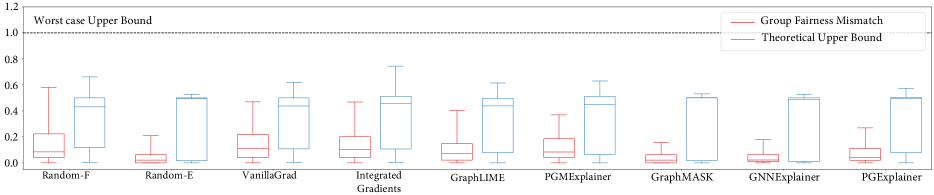
Figure 2: The empirically calculated group fairness mismatch measure (in red) and our theoretical upper bounds for group fairness mismatch (in blue) for nine explanation methods. Results show that no explanation method violate the group fairness bounds for the German credit graph dataset.

Appendix C Experiments

Datasets. We experiment with nine datasets in this work:

1) German credit graph (Agarwal et al., 2021a) has 1,000 nodes representing customers in a German bank, connected based on similarity of their credit applications. The task is to classify clients into good vs. bad credit risks considering clients’ gender as the sensitive attribute.

2) Recidivism graph (Agarwal et al., 2021a) has 18,876 nodes representing defendants released on bail that are connected based on similarity of their past criminal records and demographics. The task is to classify defendants into bail (i.e., unlikely to commit a violent crime if released) vs. no bail (i.e., likely to commit a violent crime) considering race information as the protected attribute.

3) Credit defaulter graph (Agarwal et al., 2021a) has 30,000 nodes representing individuals connected based on payment behaviors and demographics. The task is to classify individuals into credit card payment vs. no payment on time considering age as the sensitive attribute.

4) Cora dataset (McCallum et al., 2000) comprises of 2708 nodes representing scientific publications classified into one of seven classes. The data contains bibliographic records of machine learning papers that have been manually clustered into classes that refer to the same publication. The citation network consists of 5429 links. Each publication in the dataset is described by a 0/1-valued word vector indicating the absence/presence of the corresponding word from the dictionary. The dictionary consists of 1433 unique words.

5) PubMed dataset (Sen et al., 2008) consists of 19717 nodes representing scientific publications from PubMed database pertaining to diabetes classified into one of three classes. The citation network consists of 44338 links. Each publication in the dataset is described by a TF/IDF weighted word vector from a dictionary which consists of 500 unique words.

6) Citeseer dataset (Giles et al., 1998) consists of 3312 nodes representing scientific publications classified into one of six classes. The citation network consists of 4732 links. Each publication in the dataset is described by a 0/1-valued word vector indicating the absence/presence of the corresponding word from the dictionary. The dictionary consists of 3703 unique words.

7) Ogbn-mag dataset (Hu et al., 2020) is a heterogeneous graph composed of a subset of the Microsoft Academic Graph (MAG) (Wang et al., 2020). It contains four types of entities—papers (736,389 nodes), authors (1,134,649 nodes), institutions (8,740 nodes), and fields of study (59,965 nodes)—as well as four types of directed relations connecting two types of entities—an author is “affiliated with” an institution, an author “writes” a paper, a paper “cites” a paper, and a paper “has a topic of” a field of study. The task is to classify papers into 349 venues (conference or journal), given its content, references, authors, and authors’ affiliations.

8) Ogbn-arxiv citation graph (Hu et al., 2020) has 169,343 nodes representing CS arXiv papers linked based on who cites whom patterns. The task is to classify papers into 40 thematic categories, e.g., cs.AI, cs.LG, and cs.OS.

9) MUTAG dataset (Debnath et al., 1991) contains 4,337 graphs representing chemical compounds where nodes represent different atoms and edges represent chemical bonds. The graphs are labeled into two different classes according to their mutagenic effect on the Gram-negative bacterium S. typhimuriuma.

The training and testing splits for the German credit graph, Recidivism graph, and Credit defaulter graph dataset is setup following the codes released by (Agarwal et al., 2021a). For the Cora, PubMed, Citeseer, Ogbn-mag, and Ogbn-arxiv, we use the training and testing data loader provided by Hu et al. (2020). Finally, for MUTAG dataset we used the training and testing splits following (Fey and Lenssen, 2019). All datasets used in this work are publicly available and are accordingly cited.

Implementation details. All codes and datasets are available at https://anonymous.4open.science/r/GNNExEval-CC00/. We use a mutli-layer GraphSAGE model as our GNN predictor $f$ for all node classification tasks. For the German credit graph, Recidivism graph, and Credit defaulter graph datasets, we follow (Agarwal et al., 2021a) and design a model comprising of two GraphSAGE convolution layers with ReLU non-linear activation function and a fully-connected linear classification layer with Softmax activations. The hidden dimensionality of the layers is set to $16$. The same configuration was also used for Cora, PubMed and Citeseer datasets.

For the Ogbn-arxiv dataset, we follow Hu et al. (2020) and design a model comprising of three GraphSAGE convolution layers with ReLU non-linear activation function and a fully-connected linear classification layer with Softmax activations. The hidden dimensionality of the layers is set to $256$. Similarly, for Ogbn-mag dataset, we design a model comprising of three GraphSAGE convolution layers with ReLU non-linear activation function for first two layers and Softmax for the final layer. The hidden dimensionality of the layers is set to $192$.

For MUTAG dataset, we follow Fey and Lenssen (2019) and design a model comprising of three GCN convolution layers with ReLU non-linear activation function, global mean pooling layer and a fully-connected linear classification layer with Softmax activations. The hidden dimensionality of the layers is set to $16$.

Finally, for the link prediction task using Cora dataset, we use a Graph AutoEncoder model with two GraphSAGE convolution layers with ReLU activation as the encoder model and an InnerProduct layer (TorchGeometric, ) as the decoder. The hidden dimensionality of the layers is set to 16. Table 2 details the performance of the above models on their respective tasks.

Table 2: Statistics of all nine graph datasets used for node, link, and graph prediction with the GNN’s testing accuracy measured using all nodes in the test split. For the MUTAG graph classification dataset, we detail the mean nodes, edges, and degrees across all the molecules in the test split, and for the Cora-link dataset we report the AUROC for the link prediction task on the test split.

Datasets	Nodes	Edges	Node features	Sensitive Attribute	Classes	Accuracy
German credit	1,000	22,242	27	Gender	2	70.43%
Recidivism	18,876	321,308	18	Race	2	92.68%
Credit defaulter	30,000	1,436,858	13	Age	2	70.69%
Cora	2,708	5,429	1,433	N/A	7	85.78%
PubMed	19,717	44,338	500	N/A	3	93.77%
Citeseer	3,327	4,732	3,703	N/A	6	82.69%
Ogbn-mag	1,939,743	21,111,007	128	N/A	349	37.03%
Ogbn-arxiv	169,343	1,166,243	128	N/A	40	66.13%
MUTAG	19.79	17.93	7	N/A	2	76.32%
Cora-link	2,708	5,429	1,433	N/A	7	97.00%

Compute details. We use a Intel(R) Xeon(R) CPU E5-2680 with 250Gb RAM and a single NVIDIA Tesla M40 GPU for all our experiments.

Hyperparameters. For all experiments, we use normal Gaussian noise $\mathcal{N}(0,1)$ for perturbing node attributes and set the probability of perturbing an attribute dimension to 0.1. For training GraphSAGE, we use an Adam optimizer with a learning rate of $1\times 10^{-3}$, weight decay of $1\times 10^{-5}$, and the number of epochs to 1000. For the GNN explanation methods, all hyperparameters are set following the authors’ guidelines.

C.1 Results

Empirically verifying our theoretical bounds. We compare the reliability of explanation methods by computing the faithfulness, stability, counterfactual, and group fairness metrics as described in Sec. 4. The empirical and theoretical bounds for group fairness (Fig. 2) shows that no bounds were violated in our experiments. We observe consistent trend between empirically computed group fairness mismatch and theoretical bounds for all nine explanation methods, with the empirical values always lower than our theoretical upper bounds. Further, we compare the empirical and theoretical bounds for stability and counterfactual fairness for the three representative explanation methods: VanillaGrads (Fig. 3(a)), GraphLIME (Fig. 3(b)), and GraphMASK (Fig. 3(c)). Across all explanation methods, the theoretical bounds are well below the worst case upper bound with only some outlier points for stability in GraphLIME. Despite that, the median (horizontal line inside each box in Fig. 3) of the theoretical bounds are an order of magnitude smaller than that provided by the worst case upper bound.

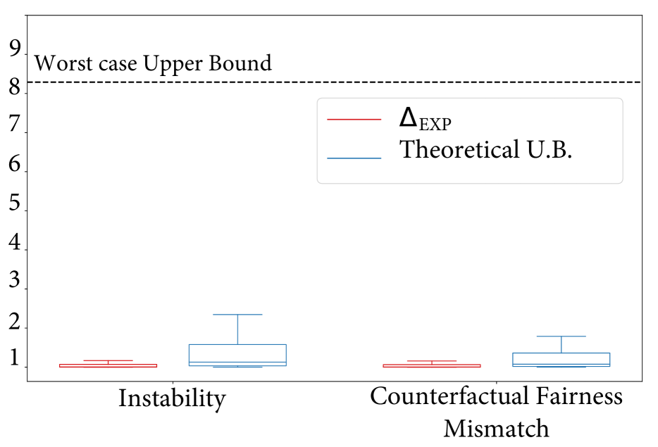
(a) VanillaGrads

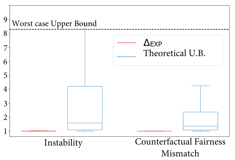
(b) GraphLIME

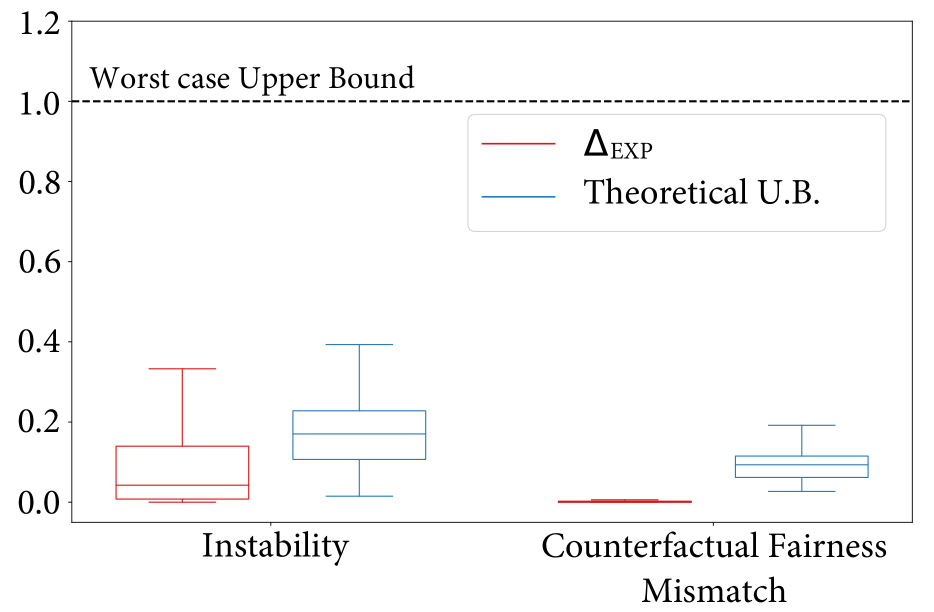
(c) GraphMASK

Figure 3: The theoretical upper bounds (in blue) for the instability and counterfactual fairness mismatch metric for (a) VanillaGrad, (b) GraphLIME, and (c) GraphMASK explanation method. Results across both properties show that the empirically calculated explanation differences $\Delta_{\text{EXP}}$ (in red) do not violate our theoretical bounds when evaluated on the German credit graph dataset.

Table 3: Systematic evaluation of GNN explanation methods (random strategies (in grey), gradient-based methods (in yellow), surrogate-based methods (in purple), and perturbation-based methods (in red)) for node classification tasks. Shown are average values of metrics and standard errors across all nodes in the test set. Arrows ($\downarrow$) indicate the direction of better performance. Note that fairness does not apply to some datasets (i.e., N/A) as they do not contain sensitive attributes.

		Evaluation metrics
Dataset	Method	Unfaithfulness ($\downarrow$)	Instability ($\downarrow$)	Fairness Mismatch ($\downarrow$)
				Counterfactual	Group
German credit graph	Random Node Features Random Edges VanillaGrad Integrated Gradients GraphLIME PGMExplainer GraphMASK GNNExplainer PGExplainer	0.208$\pm$0.011 0.049$\pm$0.004 0.185$\pm$0.010 0.199$\pm$0.011 0.158$\pm$0.009 0.131$\pm$0.007 0.034$\pm$0.003 0.046$\pm$0.004 0.074$\pm$0.006	0.386$\pm$0.006 0.375$\pm$0.001 0.222$\pm$0.010 0.254$\pm$0.019 0.096$\pm$0.013 0.183$\pm$0.006 0.270$\pm$0.008 0.377$\pm$0.001 0.367$\pm$0.004	0.387$\pm$0.006 0.375$\pm$0.001 0.137$\pm$0.007 0.210$\pm$0.018 0.063$\pm$0.008 0.185$\pm$0.006 0.006$\pm$0.001 0.359$\pm$0.002 0.360$\pm$0.009	0.165$\pm$0.015 0.061$\pm$0.009 0.154$\pm$0.012 0.150$\pm$0.012 0.114$\pm$0.010 0.129$\pm$0.010 0.046$\pm$0.006 0.060$\pm$0.009 0.079$\pm$0.001
Recidivism graph	Random Node Features Random Edges VanillaGrad Integrated Gradients GraphLIME PGMExplainer GraphMASK GNNExplainer PGExplainer	0.312$\pm$0.004 0.040$\pm$0.001 0.233$\pm$0.004 0.308$\pm$0.005 0.191$\pm$0.004 0.128$\pm$0.001 0.053$\pm$0.002 0.042$\pm$0.001 0.056$\pm$0.001	0.403$\pm$0.002 0.376$\pm$0.000 0.285$\pm$0.003 0.226$\pm$0.003 0.264$\pm$0.004 0.226$\pm$0.002 0.251$\pm$0.003 0.374$\pm$0.000 0.371$\pm$0.001	0.403$\pm$0.002 0.376$\pm$0.000 0.173$\pm$0.002 0.104$\pm$0.003 0.072$\pm$0.003 0.223$\pm$0.002 0.013$\pm$0.000 0.364$\pm$0.001 0.355$\pm$0.002	0.144$\pm$0.003 0.046$\pm$0.001 0.114$\pm$0.002 0.139$\pm$0.003 0.107$\pm$0.003 0.130$\pm$0.002 0.060$\pm$0.002 0.051$\pm$0.002 0.064$\pm$0.002
Credit defaulter graph	Random Node Features Random Edges VanillaGrad Integrated Gradients GraphLIME PGMExplainer GraphMASK GNNExplainer PGExplainer	0.098$\pm$0.002 0.020$\pm$0.001 0.092$\pm$0.002 0.147$\pm$0.003 0.038$\pm$0.002 0.283$\pm$0.002 0.012$\pm$0.001 0.021$\pm$0.001 0.028$\pm$0.001	0.426$\pm$0.002 0.376$\pm$0.000 0.333$\pm$0.002 0.140$\pm$0.002 0.225$\pm$0.004 0.156$\pm$0.002 0.036$\pm$0.002 0.375$\pm$0.000 0.364$\pm$0.001	0.424$\pm$0.002 0.376$\pm$0.000 0.171$\pm$0.002 0.069$\pm$0.001 0.063$\pm$0.003 0.154$\pm$0.002 0.004$\pm$0.000 0.366$\pm$0.000 0.348$\pm$0.002	0.045$\pm$0.002 0.017$\pm$0.001 0.042$\pm$0.002 0.053$\pm$0.002 0.018$\pm$0.001 0.161$\pm$0.003 0.010$\pm$0.001 0.019$\pm$0.001 0.022$\pm$0.001

Table 4: Systematic evaluation of GNN explanation methods (random strategies (in grey), gradient-based methods (in yellow), surrogate-based methods (in purple), and perturbation-based methods (in red)) for node classification tasks. Shown are average values of metrics and standard errors across all nodes in the test set. Arrows ($\downarrow$) indicate the direction of better performance. Note that fairness does not apply to some datasets (i.e., N/A) as they do not contain sensitive attributes.

		Evaluation metrics
Dataset	Method	Unfaithfulness ($\downarrow$)	Instability ($\downarrow$)	Fairness Mismatch ($\downarrow$)
				Counterfactual	Group
Cora	Random Node Features Random Edges VanillaGrad Integrated Gradients GraphLIME PGMExplainer GraphMASK GNNExplainer PGExplainer	0.002$\pm$0.000 0.004$\pm$0.000 0.002$\pm$0.000 0.002$\pm$0.000 0.001$\pm$0.001 0.016$\pm$0.001 0.023$\pm$0.005 0.003$\pm$0.000 0.112$\pm$0.005	0.181$\pm$0.000 0.196$\pm$0.006 0.154$\pm$0.002 0.894$\pm$0.002 0.052$\pm$0.015 0.224$\pm$0.011 0.600$\pm$0.027 0.377$\pm$0.009 0.372$\pm$0.008	N/A        N/A        N/A        N/A        N/A        N/A        N/A        N/A        N/A	N/A        N/A        N/A        N/A        N/A        N/A        N/A        N/A        N/A
PubMed	Random Node Features Random Edges VanillaGrad Integrated Gradients GraphLIME PGMExplainer GraphMASK GNNExplainer PGExplainer	0.002$\pm$0.000 0.002$\pm$0.000 0.003$\pm$0.000 0.004$\pm$0.000 0.001$\pm$0.001 0.045$\pm$0.003 0.010$\pm$0.002 0.002$\pm$0.000 0.094$\pm$0.004	0.180$\pm$0.000 0.195$\pm$0.002 0.139$\pm$0.002 0.855$\pm$0.003 0.440$\pm$0.023 0.142$\pm$0.008 0.742$\pm$0.018 0.192$\pm$0.002 0.367$\pm$0.006	N/A        N/A        N/A        N/A        N/A        N/A        N/A        N/A        N/A	N/A        N/A        N/A        N/A        N/A        N/A        N/A        N/A        N/A
Citeseer	Random Node Features Random Edges VanillaGrad Integrated Gradients GraphLIME PGMExplainer GraphMASK GNNExplainer PGExplainer	0.003$\pm$0.000 0.005$\pm$0.000 0.003$\pm$0.000 0.004$\pm$0.000 0.001$\pm$0.000 0.009$\pm$0.001 0.170$\pm$0.007 0.003$\pm$0.000 0.129$\pm$0.010	0.180$\pm$0.000 0.263$\pm$0.019 0.142$\pm$0.002 0.896$\pm$0.000 0.048$\pm$0.015 0.262$\pm$0.015 0.200$\pm$0.028 0.212$\pm$0.015 0.400$\pm$0.017	N/A        N/A        N/A        N/A        N/A        N/A        N/A        N/A        N/A	N/A        N/A        N/A        N/A        N/A        N/A        N/A        N/A        N/A
Ogbn-mag	Random Node Features Random Edges VanillaGrad Integrated Gradients GraphLIME PGMExplainer GraphMASK GNNExplainer PGExplainer	0.002$\pm$0.000 0.002$\pm$0.000 0.002$\pm$0.000 0.002$\pm$0.000 0.001$\pm$0.000 0.002$\pm$0.000 0.002$\pm$0.000 0.002$\pm$0.000 0.002$\pm$0.000	0.373$\pm$0.002 0.376$\pm$0.002 0.312$\pm$0.005 0.368$\pm$0.002 0.354$\pm$0.023 0.222$\pm$0.006 0.323$\pm$0.003 0.375$\pm$0.002 0.375$\pm$0.006	N/A        N/A        N/A        N/A        N/A        N/A        N/A        N/A        N/A	N/A        N/A        N/A        N/A        N/A        N/A        N/A        N/A        N/A
Ogbn-arxiv	Random Node Features Random Edges VanillaGrad Integrated Gradients GraphLIME PGMExplainer GraphMASK GNNExplainer PGExplainer	0.529$\pm$0.002 0.431$\pm$0.002 0.528$\pm$0.002 0.528$\pm$0.002 0.260$\pm$0.003 0.413$\pm$0.002 0.586$\pm$0.001 0.430$\pm$0.002 0.338$\pm$0.002	0.375$\pm$0.000 0.378$\pm$0.001 0.359$\pm$0.001 0.372$\pm$0.000 0.374$\pm$0.004 0.270$\pm$0.002 0.125$\pm$0.002 0.376$\pm$0.001 0.381$\pm$0.001	N/A        N/A        N/A        N/A        N/A        N/A        N/A        N/A        N/A	N/A        N/A        N/A        N/A        N/A        N/A        N/A        N/A        N/A

Table 5: Systematic evaluation of GNN explanation methods (random strategies (in grey), gradient- (in yellow), perturbation- (in red), and surrogate-based (in purple) method) for link prediction on Cora-link and graph classification on MUTAG dataset. For both tasks, VanillaGrad method perform on par or better than other explanation methods on instability, and random strategies outperform other GNN explanation methods on unfaithfulness.

Task	Method	Unfaithfulness ($\downarrow$)	Instability ($\downarrow$)
Link prediction	Random Node Features VanillaGrad Integrated Gradients GNNExplainer	0.037$\pm$0.013 0.046$\pm$0.017 0.069$\pm$0.028 0.040$\pm$0.017	0.375$\pm$0.003 0.310$\pm$0.062 0.747$\pm$0.002 0.376$\pm$0.000
Graph classification	Random Node Features Random Edges VanillaGrad Integrated Gradients PGMExplainer GNNExplainer	0.105$\pm$0.056 0.022$\pm$0.029 0.295$\pm$0.078 0.086$\pm$0.046 0.154$\pm$0.083 0.094$\pm$0.052	0.492$\pm$0.046 0.366$\pm$0.064 0.363$\pm$0.129 0.473$\pm$0.087 0.385$\pm$0.118 0.490$\pm$0.046

Figure 5: Shown are bar plots with mean values and standard errors of computed metrics for four categories of explanation methods (random strategies (in grey), gradient-based methods (in yellow), surrogate-based methods (in purple), and perturbation-based methods (in red)) across all datasets. We observe that surrogate-based explanation methods are more stable and better preserves counterfactual fairness, whereas perturbation-based explanation methods outperform others on unfaithfulness and group fairness mismatch scores.

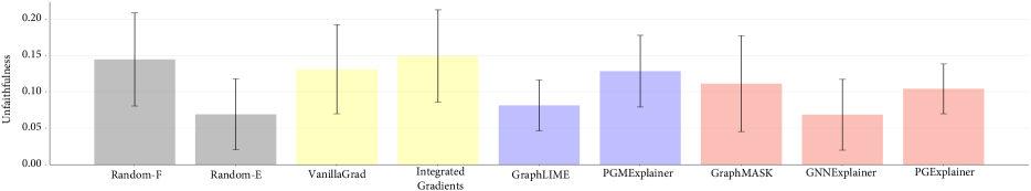
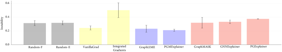
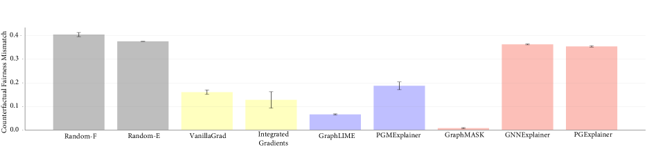
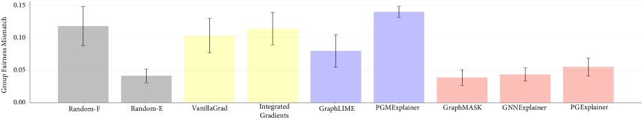
Figure 6: Shown are bar plots with mean values and standard errors of computed metrics for nine GNN explanation methods (random strategies (in grey), gradient-based methods (in yellow), surrogate-based methods (in purple), and perturbation-based methods (in red)) across all datasets. We observe that Random Edge baseline outperforms all explanation methods in terms of unfaithfulness, GraphMASK outperforms all explanation methods in preserving counterfactual and group fairness, and no explanation method satisfies all four properties.

Figure 7: Shown are bar plots with mean values and standard errors of computed metrics of random node feature explanations, random edge explanations, and explanation methods generating node- (VanillaGrad, Integrated Gradients, GraphLIME, GNNExplainer) and graph-level (PGMExplainer, GraphMASK, PGExplainer) explanations across all datasets. We observe that Random Edge explanations achieves better unfaithfulness and group fairness mismatch, whereas graph structure-based explanations perform better on stability and preserving counterfactual fairness.

References

- Agarwal et al. (2021a) Chirag Agarwal, Himabindu Lakkaraju, and Marinka Zitnik. Towards a unified framework for fair and stable graph representation learning. In UAI, 2021a.
- Agarwal et al. (2021b) Sushant Agarwal, Shahin Jabbari, Chirag Agarwal, Sohini Upadhyay, Zhiwei Steven Wu, and Himabindu Lakkaraju. Towards the unification and robustness of perturbation and gradient based explanations. In ICML, 2021b.
- Aivodji et al. (2019) Ulrich Aivodji, Hiromi Arai, Olivier Fortineau, Sébastien Gambs, Satoshi Hara, and Alain Tapp. Fairwashing: the risk of rationalization. In International Conference on Machine Learning, pages 161–170, 2019.
- Amparore et al. (2021) Elvio Amparore, Alan Perotti, and Paolo Bajardi. To trust or not to trust an explanation: using LEAF to evaluate local linear XAI methods. PeerJ Computer Science, 7:e479, 2021.
- Arya et al. (2019) Vijay Arya, Rachel KE Bellamy, Pin-Yu Chen, Amit Dhurandhar, Michael Hind, Samuel C Hoffman, Stephanie Houde, Q Vera Liao, Ronny Luss, Aleksandra Mojsilović, et al. One explanation does not fit all: A toolkit and taxonomy of AI explainability techniques. arXiv:1909.03012, 2019.
- Baldassarre and Azizpour (2019) Federico Baldassarre and Hossein Azizpour. Explainability techniques for graph convolutional networks. In ICML Workshop on Learning and Reasoning with Graph-Structured Data, 2019.
- Chen et al. (2021) Binghong Chen, Tianzhe Wang, Chengtao Li, Hanjun Dai, and Le Song. Molecule optimization by explainable evolution. In International Conference on Learning Representations, 2021.
- Chen et al. (2018) Jianbo Chen, Le Song, Martin Wainwright, and Michael Jordan. Learning to explain: An information-theoretic perspective on model interpretation. In International Conference on Machine Learning, pages 883–892. PMLR, 2018.
- Debnath et al. (1991) Asim Kumar Debnath, Rosa L Lopez de Compadre, Gargi Debnath, Alan J Shusterman, and Corwin Hansch. Structure-activity relationship of mutagenic aromatic and heteroaromatic nitro compounds. correlation with molecular orbital energies and hydrophobicity. In Journal of medicinal chemistry, 1991.
- DeYoung et al. (2020) Jay DeYoung, Sarthak Jain, Nazneen Fatema Rajani, Eric Lehman, Caiming Xiong, Richard Socher, and Byron C Wallace. Eraser: A benchmark to evaluate rationalized nlp models. In ACL, 2020.
- Dwork et al. (2012) Cynthia Dwork, Moritz Hardt, Toniann Pitassi, Omer Reingold, and Richard Zemel. Fairness through awareness. In ITSC. ACM, 2012.
- Faber et al. (2020) Lukas Faber, Amin K Moghaddam, and Roger Wattenhofer. Contrastive graph neural network explanation. In ICML Workshop on Graph Representation Learning and Beyond, 2020.
- Faber et al. (2021) Lukas Faber, Amin K. Moghaddam, and Roger Wattenhofer. When comparing to ground truth is wrong: On evaluating gnn explanation methods. In KDD, 2021.
- Fauvel et al. (2020) Kevin Fauvel, Véronique Masson, and Elisa Fromont. A performance-explainability framework to benchmark machine learning methods: Application to multivariate time series classifiers. arXiv:2005.14501, 2020.
- Fey and Lenssen (2019) Matthias Fey and Jan E. Lenssen. Fast graph representation learning with PyTorch Geometric. In ICLR Workshop on Representation Learning on Graphs and Manifolds, 2019.
- Garreau and Luxburg (2020) Damien Garreau and Ulrike Luxburg. Explaining the explainer: A first theoretical analysis of LIME. In International Conference on Artificial Intelligence and Statistics, pages 1287–1296. PMLR, 2020.
- Giles et al. (1998) C Lee Giles, Kurt D Bollacker, and Steve Lawrence. Citeseer: An automatic citation indexing system. In ACM conference on Digital libraries, 1998.
- Gouk et al. (2021) Henry Gouk, Eibe Frank, Bernhard Pfahringer, and Michael J Cree. Regularisation of neural networks by enforcing lipschitz continuity. In Machine Learning. Springer, 2021.
- Gretton et al. (2005) Arthur Gretton, Olivier Bousquet, Alex Smola, and Bernhard Schölkopf. Measuring statistical dependence with hilbert-schmidt norms. In ICALT, 2005.
- Han et al. (2021) Zhen Han, Peng Chen, Yunpu Ma, and Volker Tresp. Explainable subgraph reasoning for forecasting on temporal knowledge graphs. In International Conference on Learning Representations, 2021.
- Hardt et al. (2016) Moritz Hardt, Eric Price, and Nathan Srebro. Equality of opportunity in supervised learning. In NeurIPS, 2016.
- Hu et al. (2020) Weihua Hu, Matthias Fey, Marinka Zitnik, Yuxiao Dong, Hongyu Ren, Bowen Liu, Michele Catasta, and Jure Leskovec. Open graph benchmark: Datasets for machine learning on graphs. In NeurIPS, 2020.
- Huang et al. (2020) Qiang Huang, Makoto Yamada, Yuan Tian, Dinesh Singh, Dawei Yin, and Yi Chang. Graphlime: Local interpretable model explanations for graph neural networks. arXiv, 2020.
- Jeyakumar et al. (2020) Jeya Vikranth Jeyakumar, Joseph Noor, Yu-Hsi Cheng, Luis Garcia, and Mani Srivastava. How can I explain this to you? an empirical study of deep neural network explanation methods. Advances in Neural Information Processing Systems, 2020.
- Jin et al. (2020) Guangyin Jin, Qi Wang, Cunchao Zhu, Yanghe Feng, Jincai Huang, and Jiangping Zhou. Addressing crime situation forecasting task with temporal graph convolutional neural network approach. In ICMTMA. IEEE, 2020.
- Lakkaraju et al. (2020) Himabindu Lakkaraju, Nino Arsov, and Osbert Bastani. Robust and stable black box explanations. In ICML. PMLR, 2020.
- Li et al. (2021) Michelle M Li, Kexin Huang, and Marinka Zitnik. Representation learning for networks in biology and medicine: Advancements, challenges, and opportunities. arXiv, 2021.
- Lin et al. (2021) Wanyu Lin, Hao Lan, and Baochun Li. Generative causal explanations for graph neural networks. In ICML, 2021.
- Liu et al. (2021) Yang Liu, Sujay Khandagale, Colin White, and Willie Neiswanger. Synthetic benchmarks for scientific research in explainable machine learning. In NeurIPS Datasets and Benchmarks, 2021.
- Lucic et al. (2021) Ana Lucic, Maartje ter Hoeve, Gabriele Tolomei, Maarten de Rijke, and Fabrizio Silvestri. Cf-gnnexplainer: Counterfactual explanations for graph neural networks. arXiv, 2021.
- Luo et al. (2020) Dongsheng Luo, Wei Cheng, Dongkuan Xu, Wenchao Yu, Bo Zong, Haifeng Chen, and Xiang Zhang. Parameterized explainer for graph neural network. In NeurIPS, 2020.
- McCallum et al. (2000) Andrew Kachites McCallum, Kamal Nigam, Jason Rennie, and Kristie Seymore. Automating the construction of internet portals with machine learning. In Information Retrieval, 2000.
- Pareja et al. (2020) Aldo Pareja, Giacomo Domeniconi, Jie Chen, Tengfei Ma, Toyotaro Suzumura, Hiroki Kanezashi, Tim Kaler, Tao Schardl, and Charles Leiserson. EvolveGCN: Evolving graph convolutional networks for dynamic graphs. In AAAI, 2020.
- Peng and Ding (2005) Hanchuan Peng and Chris Ding. Minimum redundancy and maximum relevance feature selection and recent advances in cancer classification. In Feature Selection for Data Mining, 2005.
- Pope et al. (2019) Phillip E Pope, Soheil Kolouri, Mohammad Rostami, Charles E Martin, and Heiko Hoffmann. Explainability methods for graph convolutional neural networks. In CVPR, 2019.
- Reams (1999) Robert Reams. Hadamard inverses, square roots and products of almost semidefinite matrices. In Linear Algebra and its Applications, 1999.
- Sanchez-Lengeling et al. (2020) Benjamin Sanchez-Lengeling, Jennifer Wei, Brian Lee, Emily Reif, Peter Wang, Wesley Wei Qian, Kevin McCloskey, Lucy Colwell, and Alexander Wiltschko. Evaluating attribution for graph neural networks. In NeurIPS, 2020.
- Schlichtkrull et al. (2021) Michael Sejr Schlichtkrull, Nicola De Cao, and Ivan Titov. Interpreting graph neural networks for nlp with differentiable edge masking. In ICLR, 2021.
- Schnake et al. (2020) Thomas Schnake, Oliver Eberle, Jonas Lederer, Shinichi Nakajima, Kristof T Schütt, Klaus-Robert Müller, and Grégoire Montavon. Higher-order explanations of graph neural networks via relevant walks. arXiv, 2020.
- Sen et al. (2008) Prithviraj Sen, Galileo Namata, Mustafa Bilgic, Lise Getoor, Brian Galligher, and Tina Eliassi-Rad. Collective classification in network data. In AI magazine, 2008.
- Simonyan et al. (2014) Karen Simonyan, Andrea Vedaldi, and Andrew Zisserman. Deep inside convolutional networks: Visualising image classification models and saliency maps. In Workshop at ICLR, 2014.
- Sundararajan et al. (2017) Mukund Sundararajan, Ankur Taly, and Qiqi Yan. Axiomatic attribution for deep networks. In ICML, 2017.
- (43) TorchGeometric. pytorch geometric 2.0.0 documentation. https://pytorch-geometric.readthedocs.io/en/latest/modules/nn.html#torch_geometric.nn.models.InnerProductDecoder. (Accessed on 09/09/2021).
- Vignac et al. (2020) Clement Vignac, Andreas Loukas, and Pascal Frossard. Building powerful and equivariant graph neural networks with structural message-passing. In NeurIPS, 2020.
- Vu and Thai (2020) Minh N Vu and My T Thai. Pgm-explainer: Probabilistic graphical model explanations for graph neural networks. In NeurIPS, 2020.
- Wang et al. (2020) Kuansan Wang, Zhihong Shen, Chiyuan Huang, Chieh-Han Wu, Yuxiao Dong, and Anshul Kanakia. Microsoft academic graph: When experts are not enough. In Quantitative Science Studies, 2020.
- Yamada et al. (2014) Makoto Yamada, Wittawat Jitkrittum, Leonid Sigal, Eric P Xing, and Masashi Sugiyama. High-dimensional feature selection by feature-wise kernelized lasso. In Neural computation, 2014.
- Ying et al. (2019) Rex Ying, Dylan Bourgeois, Jiaxuan You, Marinka Zitnik, and Jure Leskovec. Gnnexplainer: Generating explanations for graph neural networks. In NeurIPS, 2019.
- Yuan et al. (2020a) Hao Yuan, Jiliang Tang, Xia Hu, and Shuiwang Ji. Xgnn: Towards model-level explanations of graph neural networks. In KDD, 2020a.
- Yuan et al. (2020b) Hao Yuan, Haiyang Yu, Shurui Gui, and Shuiwang Ji. Explainability in graph neural networks: A taxonomic survey. arXiv, 2020b.
- Yun et al. (2019) Seongjun Yun, Minbyul Jeong, Raehyun Kim, Jaewoo Kang, and Hyunwoo J Kim. Graph transformer networks. NeurIPS, 2019.
- Zhao and Gordon (2019) Han Zhao and Geoffrey J Gordon. Inherent tradeoffs in learning fair representations. In NeurIPS, 2019.
- Zitnik et al. (2018) Marinka Zitnik, Monica Agrawal, and Jure Leskovec. Modeling polypharmacy side effects with graph convolutional networks. In Bioinformatics, 2018.