The stellar mass - physical effective radius relation for dwarf galaxies in low-density environments

Abstract

The scaling relation between stellar mass ($M_{*}$) and physical effective radius ($r_{e}$) has been well-studied using wide spectroscopic surveys. However, these surveys suffer from severe surface brightness incompleteness in the dwarf galaxy regime, where the relation is poorly constrained. In this study, I use a Bayesian empirical model to constrain the power-law exponent $\beta$ of the $M_{*}$-$r_{e}$ relation for late-type dwarfs ($10^{7}$$\leq$$M_{*}$/$\mathrm{M_{\odot}}$$\leq$$10^{9}$) using a sample of 188 isolated low surface brightness (LSB) galaxies, accounting for observational incompleteness. Surprisingly, the best-fitting model ($\beta$=0.40$\pm$0.07) indicates that the relation is significantly steeper than would be expected from extrapolating canonical models into the dwarf galaxy regime. Nevertheless, the best fitting $M_{*}$-$r_{e}$ relation closely follows the distribution of known dwarf galaxies. These results indicate that extrapolated canonical models over-predict the number of large dwarf (i.e. LSB) galaxies, including ultra-diffuse galaxies (UDGs), explaining why they are over-produced by some semi-analytic models. The best-fitting model also constrains the power-law exponent of the physical size distribution of UDGs to $n\mathrm{[dex^{-1}]}\propto$$~{}r_{e}^{3.54\pm 0.33}$, consistent to within 1$\sigma$ of the corresponding value in cluster environments and with the theoretical scenario in which UDGs occupy the high-spin tail of the normal dwarf galaxy population.

1 Introduction

The advent of wide-field spectroscopic surveys has allowed systematic distance measurements of millions for galaxies, thus enabling the scaling relation between stellar mass ($M_{*}$) and physical effective radius to be determined empirically (Shen et al., 2003; van der Wel et al., 2014; Lange et al., 2015). This relation plays an important role in understanding galaxy formation theoretically, forming a basic ingredient of semi-analytical models (e.g. Somerville & Primack, 1999) as well as a basis of comparison for cosmological simulations (e.g. Buck et al., 2020; Davison et al., 2020). However, spectroscopic surveys invariably suffer from completeness effects, meaning the relation is poorly constrained in the dwarf galaxy regime ($M_{*}$$\leq$$10^{9}$$\mathrm{M_{\odot}}$) where galaxies typically have lower surface brightness (Martin et al., 2019).

Low surface brightness galaxies (LSBGs), characterised by surface brightness levels fainter than 24 magnitudes per square-arcsecond averaged within their effective radii, are often completely missed in spectroscopic surveys (Wright et al., 2017). These galaxies are uncommonly large for their stellar masses, the most extreme of which ($r_{e}$$\gtrsim$1.5 kpc) being known as “ultra-diffuse galaxies” (UDGs, van Dokkum et al., 2015).

LSBGs can form and evolve through a variety of processes (e.g. Jackson et al., 2020), which can be either secular (proceeding without external influence) or environmentally-driven. Secular channels are more influential for field galaxy populations owing to the decreased environmental density. One example is supernovae feedback, which can enlarge normal dwarf galaxies, thereby turning them into LSBGs (Di Cintio et al., 2017). Higher than average halo spin parameters can also create dwarf galaxies with large sizes (Amorisco & Loeb, 2016; Rong et al., 2017; Tremmel et al., 2020). One prediction from this scenario is that the distribution of effective radii among the field LSBG population should follow a power-law with an exponent similar to that measured in cluster environments (van der Burg et al., 2016). Recent kinematic studies have indicated that the theory is viable for UDGs in lower density environments (Mancera Piña et al., 2020). However, a systematic study of this field population has yet to be performed.

Distances to LSBGs in nearby galaxy groups and clusters can be estimated by associating them with their environment. Prohibitive difficulties in measuring distances to more isolated galaxies (e.g. Trujillo et al., 2019) have caused the field population to remain poorly understood. This problem will not be fully addressed by the next generation of all-sky extragalactic spectroscopic surveys (e.g. from 4MOST), which will not provide spectroscopic distance estimates for large samples of LSB galaxies because they are too faint to meet survey selection criteria. Other techniques such as surface brightness fluctuations (Greco et al., 2020) will not be useful for galaxies far outside of the local group.

In this paper, I use an empirical model to constrain the stellar mass - effective radius relation in the dwarf galaxy regime using a method that implicitly accounts for surface brightness incompleteness. This is achieved by fitting the model to the sample of field LSBGs recently obtained by Prole et al. (2021) (hereafter P21). I investigate whether the model is consistent with the theoretical predictions for UDGs from Amorisco & Loeb (2016) and corresponding measurements inside galaxy clusters (van der Burg et al., 2016) as well as groups (van der Burg et al., 2017). While no distance measurements are available for the observed sample, the model overcomes this problem by assuming the galaxies are distributed smoothly along with the matter in the Universe.

Throughout this paper, surface brightnesses are always given in units of magnitudes per square arc-second and the AB magnitude system is used. $\Lambda$CDM cosmology is assumed, with $\Omega_{\mathrm{m}}$=0.3, $\Omega_{\Lambda}$=0.7 and H₀=70 kms^-1Mpc^-1.

2 Data

The publicly-available LSBG catalogue from P21 is used in this study. In particular, the subset of blue LSBGs are selected because they show no correlation with local structure and may be considered to exist in low-density environments. These galaxies were identified in deep optical imaging from HSC-SSP PDR2 (Aihara et al., 2019) and have $r$-band structural parameter measurements based on single component 2D Sérsic fits. The sample are selected to have 24$\leq$$\bar{\mu}_{e}$$<$27 and 3″$\leq$$\bar{r}_{e}$$<$10″, where $\bar{\mu}_{e}$ and $\bar{r}_{e}$ are the measured apparent surface brightness averaged within the effective radius and the angular circularised effective radius respectively. A further selection cut is applied in colour: 0$\leq$$\bar{c}$$<$0.42, where $\bar{c}$ is the observer-frame $(g-r)$ colour in magnitudes. These criteria leave 188 galaxies in the sample. The maximum Sérsic index ($n$) of the sample is 2.2. The sample are likely to be local ($z$$<$0.2), with the main bulk of sources being much closer ($z$$<$0.1). For a full description of the sample, selection criteria and distance arguments, the reader is referred to P21.

3 Model

The objective of the statistical model is to reproduce the joint distribution of observed quantities from the P21 sample given a set of model hyper parameters $\boldsymbol{\theta}$:

$$p_{obs}(\bar{\mu}_{e},\bar{r}_{e},\bar{c}~{}|\boldsymbol{\theta})$$ (1)

In order to achieve this, we must model the underlying joint distribution of physical properties that are $observed$ given the selection criteria of P21:

$$p_{obs}(M_{*},z,\hat{r}_{e},\hat{c}~{}|\boldsymbol{\theta})\propto\epsilon(M_{*},z,\hat{r}_{e},\hat{c})p(M_{*},z,\hat{r}_{e},\hat{c}~{}|\boldsymbol{\theta})$$ (2)

where $M_{*}$ is the stellar mass, $z$ is the redshift, $\hat{r}_{e}$ is the physical circularised effective radius and $\hat{c}$ is the rest-frame $(g-r)$ colour. $\epsilon$ is the fraction of recovered galaxies given the selection criteria used in P21, parametrised as a function of $\bar{\mu}_{e}$, $\bar{r}_{e}$.

Empirical relations pertaining to late-type galaxies are used throughout the model. This is justified because $\epsilon$=0 for galaxies that do not satisfy the selection criteria, and the selection criteria of P21 target the late type population. The reader is referred to the selection criteria of “late-type” galaxies discussed in Baldry et al. (2012) and Lange et al. (2015) which are consistent with the sample in this study (blue colours and $n$$<$2.5).

3.1 Redshift distribution

The results of P21 showed that the observed LSBG sample do not correlate spatially with local structure. I therefore assume that the spatial distribution of these galaxies can be expected, when averaged over large-enough areas, to follow the mean cosmological distribution of mass within the volume element, such that:

$$p(z)\propto\Omega_{m}(z)\rho_{\mathrm{crit}}(z)\frac{dV}{dz}$$ (3)

where $\Omega_{m}$ is the matter-density parameter, $\rho_{\mathrm{crit}}$ is the critical density of the Universe and $\frac{dV}{dz}$ is a term that is proportional to the cosmological volume element.

I also make assumption that the redshift distribution $p(z)$ is independently distributed from the physical properties of the galaxies. This is justified if the observed sample are isolated and local enough such that any redshift evolution is negligible. Therefore, it is possible to write:

$$p(M_{*},z,\hat{r}_{e},\hat{c})=p(M_{*},\hat{r}_{e},\hat{c})p(z)$$ (4)

3.2 Stellar mass distribution

The galaxy stellar mass function (SMF) is well-constrained for late-type galaxies well into the dwarf galaxy regime (Baldry et al., 2012; Sedgwick et al., 2019b). The SMF is commonly parametrised using a Schechter function:

$$p(M_{*}|M_{0},\alpha)\propto\mathrm{exp}\left(\frac{-M_{*}}{M_{0}}\right)\left(\frac{M_{*}}{M_{0}}\right)^{\alpha}$$ (5)

where $M_{0}$ is the “mass-break” parameter and $\alpha$ is the “faint end slope” which governs the relative abundance of low-mass galaxies. Fiducial values are $\alpha=-1.45$, $M_{0}=10.56\mathrm{M_{\odot}}$ (Sedgwick et al., 2019a). In this work, $M_{0}$ is fixed to this value, resulting in a single free parameter, $\alpha$, to govern the SMF.

3.3 Stellar mass - effective radius relation

The scaling relation between stellar mass and physical size for late-type galaxies has been well-constrained for stellar masses greater than around $10^{9}$$\mathrm{M_{\odot}}$ (Shen et al., 2003; van der Wel et al., 2014; Lange et al., 2015, figure 3). I adopt the results from Shen et al. (2003) as they fit circularised effective radii as opposed to semi-major effective-radii, while also fitting for the intrinsic scatter in the relation.

An interesting property of this model is that it reduces to a simple form for galaxies with stellar masses lower than $\sim$$10^{10}\mathrm{M_{\odot}}$: $\hat{r}_{e}$$\propto$$M_{*}$^γ, $\sigma_{\ln{\hat{r}_{e}}}$=$const$, where $\sigma_{\ln{\hat{r}_{e}}}$ quantifies the log-normal scatter in the relation. However, this model is not constrained for galaxies less massive than $M_{*}$$\sim$$10^{9}$$\mathrm{M_{\odot}}$ owing to incompleteness in the observed sample used to measure it. I therefore consider a simple power-law extension to the Shen et al. (2003) model for galaxies lower than this limit:

$$\log(\hat{r}_{e},M_{*}<10^{9}\mathrm{M_{\odot}})=a(M_{*}/\mathrm{M_{\odot}})^{\beta}$$ (6)

where $\beta$ is the power law exponent that governs the sizes of dwarf galaxies at a given stellar mass, and $a$ is chosen to keep the $M_{*}$-$\hat{r}_{e}$ relation continuous. $\beta$ is left as a free parameter of the model. Setting $\beta$=$\gamma$=0.14 is equivalent to an extrapolation of the Shen et al. (2003) relation. I make the assumption that $\sigma_{\ln{\hat{r}_{e}}}$=$const$ can be extrapolated to lower masses than $10^{9}$$\mathrm{M_{\odot}}$.

3.4 Rest frame colours

The rest-frame colours of galaxies correlate with their stellar masses; higher mass galaxies are typically redder. This is an important effect to model because of the colour selection used in P21. I adopt the empirical relation between rest-frame ($g-r$) colour and stellar mass using data obtained for the GAMA survey (Taylor et al., 2011). The data are well-modelled by a mean trend plus constant scatter term ($\sim$$0.1$ mag). However, for low stellar masses ($<10^{9}$$\mathrm{M_{\odot}}$), the GAMA sample suffers from surface brightness incompleteness (Wright et al., 2017). This is important because higher surface brightness dwarf galaxies are typically bluer than their LSB counterparts. I make the assumption that the rest-frame ($g-r$) colours of dwarf galaxies can be modelled by a normal distribution with mean 0.35 and a standard deviation of $\sim$$0.1$ mag, in agreement with the sample of P21 as well as the field UDGs of Leisman et al. (2017). The stellar mass-colour relation is naturally continuous given these assumptions. The importance of this assumption is discussed in $\S$4.

3.5 Sampling

It is not easy to evaluate the model (equation 2) directly because of its high-dimensionality and non-parametric description of measurement errors (see $\S$3.7). The alternative approach adopted here is to sample from the model using Marcov chain Monte Carlo (MCMC). Specifically, ensemble sampling via emcee is used (Foreman-Mackey et al., 2013). Given a set of model hyper parameters $\boldsymbol{\theta}$=($\alpha$, $\beta$), 200 walkers are used to obtain 2 million total samples of ($M_{*}$, $z$, $\hat{r}_{e}$, $\hat{c}$), after discarding the initial 1000 samples from each walker. The model is adequately sampled given these settings: the sampling chain runs for $\sim$200 times the autocorrelation time for each parameter. No hard parameter limits are imposed during sampling (other than the selection cuts discussed in $\S$2) since the recovery fraction $\epsilon$ naturally imposes such limits.

3.6 Distance projection

The model needs to convert physical quantities ($M_{*}$, $z$, $\hat{r}_{e}$, $\hat{c}$) into observables ($\bar{\mu}_{e}$, $\bar{r}_{e}$, $\bar{c}$) in order to compare with observations and to evaluate the recovery fraction $\epsilon$. Physical sizes are projected to angular sizes using the cosmological angular diameter distance. Stellar masses are converted into absolute magnitudes as a function of rest-frame colour and stellar mass using the results of Taylor et al. (2011). Cosmological surface brightness dimming is accounted for by using the luminosity distance in combination wit the angular diameter distance when projecting in redshift. $k$-corrections are assigned to model samples based on their redshift and rest-frame colour in accordance with Chilingarian et al. (2010).

3.7 Measurement error

Measurement errors are modelled using the artificial source injections from P21: The catalogue is binned two-dimensionally in $\tilde{\mu}_{e}$, $\tilde{r}_{e}$, the intrinsic (free from measurement error) observer-frame surface brightness and angular, circularised effective radii. Model samples are assigned relative errors in these quantities by directly assigning them a fractional error from a random artificial source in the same bin. This approach is non-parametric and accounts for both random and systematic uncertainties as a function of $\tilde{\mu}_{e}$, $\tilde{r}_{e}$. The ability to include the effects of measurement error this way is one of the key advantages of sampling the model rather than evaluating it analytically.

4 Results

All three observed quantities ($\bar{\mu}_{e}$, $\bar{r}_{e}$and $\bar{c}$) are used to fit the model to the data. This prompts a 3D likelihood term of the form:

$$\mathcal{L}(\boldsymbol{\theta})=\prod_{i}p(\bar{\mu}_{e,i},\bar{r}_{e,i},\bar{c}_{i}~{}|\boldsymbol{\theta})$$ (7)

where $i$ loops over the observations. The probability density $p(\bar{\mu}_{e,i},\bar{r}_{e,i},\bar{c}_{i}~{}|\boldsymbol{\theta})$ is estimated from the model samples using a 3D Gaussian kernel. Since kernel density estimation (KDE) performs poorly on bounded problems (i.e. selection cuts) with heavily skewed distributions, as is the case here, a box-cox transform (Box & Cox, 1964) is first applied to both the observations and model samples. This improves the ability of the KDE to represent the probability density at the selection boundaries.

Sampling 2 million times from equation 2 is computationally demanding. This means that it is not practical to use a MCMC approach to evaluate equation 7 for many sets of $\boldsymbol{\theta}$. I therefore adopt a grid-based approach for exploring the likelihood space. In this method, a uniformly sampled grid of hyper parameters $\boldsymbol{\theta}$_i,j is considered, with the following range: -1.65$\leq$$\alpha$$<$1.25 in steps of 0.025, and 0.2$\leq$$\beta$$<$0.8 in steps of 0.025.

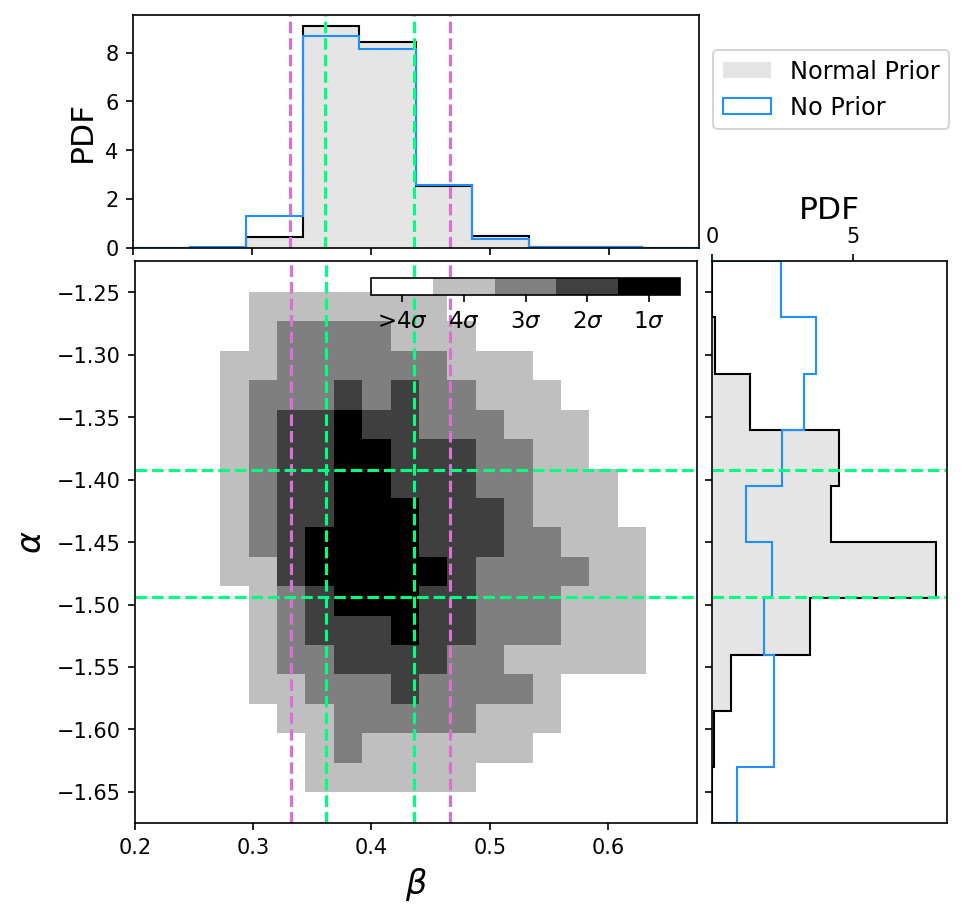
Figure 1: The posterior distribution as a function of hyper parameters $\alpha$ (faint end slope of the SMF) and $\beta$ (power-law exponent of the $M_{*}$-$\hat{r}_{e}$ relation in the dwarf galaxy regime). The marginal posteriors are shown for a uniform (blue histograms) and normal prior (grey histograms). The marginalised $\pm$1$\sigma$ intervals are shown in green. The pink lines show the uncertainty on $\beta$ after taking additional systematic uncertainties into account.

The faint end slope the SMF as measured by Sedgwick et al. (2019a) is well-constrained and includes the contribution from the LSBG population over the mass range considered here. This motivates a normal prior on $\alpha$ with mean a mean of -1.45 and standard deviation of 0.05 that is multiplied with the likelihood to form the posterior distribution. The prior is found to be influential for constraining $\alpha$, which is otherwise unconstrained by the observations (figure 1). However, it does not significantly impact the marginalised posterior for $\beta$ as compared to a uniform prior over the fitting range.

The posterior distribution implies $\beta$=0.40$\pm$0.04 and $\alpha$=-1.44$\pm$0.05, i.e. the prior distribution in $\alpha$ is recovered. Samples from the best-fitting model are shown in figure 2. The marginalised distributions in the model observed quantities $\bar{\mu}_{e}$, $\bar{r}_{e}$, $\bar{c}$ are consistent with observations, with KS statistic $p$-values$>$0.1. The uncertainties from the model fit are verified by resampling the best-fitting model with the same sample size as the observed dataset several times.

The majority ($78\pm 5\%$) of samples in the best-fitting model are dwarf galaxies, with $M_{*}$$\leq$$10^{9}$$\mathrm{M_{\odot}}$. The result indicates that the observations do not contain many galaxies with stellar masses lower than $\sim$$10^{7}$$\mathrm{M_{\odot}}$. Furthermore, $84\pm 1\%$ of samples are UDGs according to the van der Burg et al. (2016) definition. As expected, the majority of galaxies are local, with $z$$<$0.1.

As mentioned in $\S$3.4, the colour model adopted for dwarf galaxies introduces a systematic error in the model. The observed samples of P21 and Leisman et al. (2017) suggest the mean of this distribution is at $(g-r)$=0.35. However, bluer galaxies tend to be of higher surface brightness at fixed stellar mass, meaning that assumptions based solely off LSB samples can be prone to bias. Making the mean bluer actually results in a steepening of the slope $\beta$, making the result more extreme, but this is disfavoured by the sizes of dwarf galaxies measured in the GAMA survey (figure 3). Adopting a redder mean value of $(g-r)$$\sim$0.4 (as suggested by some models of UDG formation Rong et al., 2017), makes the $M_{*}$-$\hat{r}_{e}$ relation shallower, but this reduces the quality of the fit as quantified by the KS statistic. The net effect of varying the colour model is to introduce an additional uncertainty in $\beta$ of $\sim$0.05, which is incorporated into the final result: $\beta$=0.40$\pm$0.07.

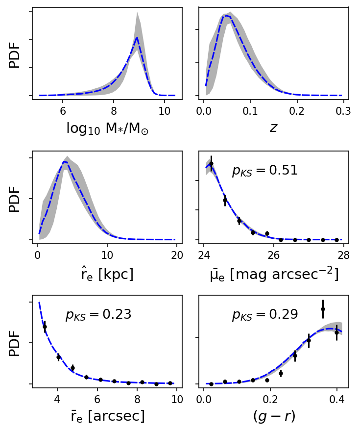
Figure 2: Predicted observations from the best-fitting model (blue lines) and 90% confidence interval (grey regions) vs the observations (black points) given the selection efficiency from the P21 survey. The quantities $M_{*}$, $z$ and $\hat{r}_{e}$ are not observed but are constrained by the model.

Figure 3: Stellar mass to circularised effective radius relation for late-type GAMA galaxies (greyscale), overlayed with the Shen et al. (2003) model (extrapolated below $10^{9}$ $\mathrm{M_{\odot}}$) and Lange et al. (2015) model, which has been converted into circularised effective radii assuming a mean axis-ratio of 0.7. The 1$\sigma$ confidence interval in the best-fit model is shown in dark blue, with the 1$\sigma$ scatter in light blue. HI-bearing UDGs from Leisman et al. (2017) are also shown. The GAMA data are not used to fit the model.

5 Discussion

5.1 Stellar mass - size relation

The true slope of the mass - size relation has not been established in the dwarf galaxy regime because of surface brightness incompleteness, so a natural expectation would be for the slope measured in this work to be shallower than that of canonical models measured using higher surface brightness samples. However, it has not been established if extrapolations of the Shen et al. (2003) or Lange et al. (2015) models are appropriate for dwarf galaxies. In point of fact, it is clear from figure 3 that such extrapolations already significantly over-estimate the sizes of dwarf galaxies present in the GAMA catalogue.

Indeed, the best-fitting model implies $\beta$ is significantly (3$\sigma$) steeper than would be expected from such extrapolations. Furthermore, the best-fitting model presented here appears to overlap with the mean trend of higher surface brightness dwarf galaxies in the GAMA catalogue (figure 3), meaning that the LSB galaxy population exists in the high-$\hat{r}_{e}$ tail of the mass-size relation and no significant alteration is required to the mean trend that would be measured directly from higher surface brightness dwarfs. This is consistent with the results of Jones et al. (2018), who showed HI-rich UDGs constitute a only a small fraction ($\leq$6%) of detectable HI-bearing dwarf galaxies, with the majority being much smaller in size.

This discrepancy between the best-fit model and extrapolated canonical models could be the reason why the semi-analytic model used by Jones et al. (2018), who used the extrapolated Lange et al. (2015) relation, over-produces field UDGs. This idea is compounded by the position of the Leisman et al. (2017) UDGs in figure 3, which appear as 2$\sigma$ outliers from the mean relation. Incidentally, this is fully consistent with the alternative definition of UDGs introduced by Lim et al. (2020), who defined them as significant outliers from empirical galaxy scaling relations.

5.2 Ultra-diffuse galaxy size distribution

The size distribution of UDGs can be obtained from the best fitting model after discounting selection effects (i.e. ignoring the recovery fraction $\epsilon$) and selecting only UDGs. A power-law model is fit to the resulting distribution of $\hat{r}_{e}$ (figure 4). The best-fitting power law is $n[\mathrm{dex^{-1}}]\propto\hat{r}_{e}^{3.54\pm 0.33}$, entirely consistent with the value measured for UDGs in clusters (van der Burg et al., 2016), but inconsistent with the value measured for those in galaxy groups (van der Burg et al., 2017).

The result is also consistent with the value predicted for field UDGs by Amorisco & Loeb (2016), indicating higher than average halo spin parameters could be the dominant channel for UDG production. It is clear from figure 4 that the power-law description may not provide the most precise representation of the UDG size distribution predicted by the model, which is qualitatively consistent with the small departure from the power-law visible in the results of Amorisco & Loeb (2016).

Figure 4: Power-law fit to model UDG size distribution in comparison with literature values (van der Burg et al., 2016; van der Burg et al., 2017). The new result is consistent with UDGs in clusters and those theoretically expected in the field (Amorisco & Loeb, 2016).

6 Data Availability

The observed sample underlying this article is publicly available (P21). The full code used to produce the results presented here is publicly available at https://github.com/danjampro/udg-sizes.

7 Acknowledgements

I would like to thank the reviewer for their significant contribution to the quality of this article. D.P. acknowledges funding from an Australian Research Council Discovery Program grant DP190102448.

References

- Aihara et al. (2019) Aihara H., et al., 2019, PASJ, p. 106
- Amorisco & Loeb (2016) Amorisco N. C., Loeb A., 2016, MNRAS, 459, L51
- Baldry et al. (2012) Baldry I. K., et al., 2012, MNRAS, 421, 621
- Box & Cox (1964) Box G. E. P., Cox D. R., 1964, Journal of the Royal Statistical Society. Series B (Methodological), 26, 211
- Buck et al. (2020) Buck T., Obreja A., Macciò A. V., Minchev I., Dutton A. A., Ostriker J. P., 2020, MNRAS, 491, 3461
- Chilingarian et al. (2010) Chilingarian I. V., Melchior A.-L., Zolotukhin I. Y., 2010, MNRAS, 405, 1409
- Davison et al. (2020) Davison T. A., Norris M. A., Pfeffer J. L., Davies J. J., Crain R. A., 2020, MNRAS, 497, 81
- Di Cintio et al. (2017) Di Cintio A., Brook C. B., Dutton A. A., Macciò A. V., Obreja A., Dekel A., 2017, MNRAS, 466, L1
- Foreman-Mackey et al. (2013) Foreman-Mackey D., Hogg D. W., Lang D., Goodman J., 2013, Publications of the Astronomical Society of the Pacific, 125, 306
- Greco et al. (2020) Greco J. P., van Dokkum P., Danieli S., Carlsten S. G., Conroy C., 2020, arXiv e-prints, p. arXiv:2004.07273
- Jackson et al. (2020) Jackson R. A., et al., 2020, arXiv e-prints, p. arXiv:2007.06581
- Jones et al. (2018) Jones M. G., Papastergis E., Pandya V., Leisman L., Romanowsky A. J., Yung L. Y. A., Somerville R. S., Adams E. A. K., 2018, A&A, 614, A21
- Lange et al. (2015) Lange R., et al., 2015, MNRAS, 447, 2603
- Leisman et al. (2017) Leisman L., et al., 2017, ApJ, 842, 133
- Lim et al. (2020) Lim S., et al., 2020, ApJ, 899, 69
- Mancera Piña et al. (2020) Mancera Piña P. E., et al., 2020, MNRAS, 495, 3636
- Martin et al. (2019) Martin G., et al., 2019, MNRAS, 485, 796
- Prole et al. (2021) Prole D. J., van der Burg R. F. J., Hilker M., Spitler L. R., 2021, MNRAS, 500, 2049
- Rong et al. (2017) Rong Y., Guo Q., Gao L., Liao S., Xie L., Puzia T. H., Sun S., Pan J., 2017, MNRAS, 470, 4231
- Sedgwick et al. (2019a) Sedgwick T. M., Baldry I. K., James P. A., Kelvin L. S., 2019a, arXiv e-prints, p. arXiv:1909.04535
- Sedgwick et al. (2019b) Sedgwick T. M., Baldry I. K., James P. A., Kelvin L. S., 2019b, MNRAS, 484, 5278
- Shen et al. (2003) Shen S., Mo H. J., White S. D. M., Blanton M. R., Kauffmann G., Voges W., Brinkmann J., Csabai I., 2003, MNRAS, 343, 978
- Somerville & Primack (1999) Somerville R. S., Primack J. R., 1999, Monthly Notices of the Royal Astronomical Society, 310, 1087
- Taylor et al. (2011) Taylor E. N., et al., 2011, MNRAS, 418, 1587
- Tremmel et al. (2020) Tremmel M., Wright A. C., Brooks A. M., Munshi F., Nagai D., Quinn T. R., 2020, MNRAS, 497, 2786
- Trujillo et al. (2019) Trujillo I., et al., 2019, MNRAS, 486, 1192
- Wright et al. (2017) Wright A. H., et al., 2017, MNRAS, 470, 283
- van Dokkum et al. (2015) van Dokkum P. G., Abraham R., Merritt A., Zhang J., Geha M., Conroy C., 2015, ApJ, 798, L45
- van der Burg et al. (2016) van der Burg R. F. J., Muzzin A., Hoekstra H., 2016, A&A, 590, A20
- van der Burg et al. (2017) van der Burg R. F. J., et al., 2017, A&A, 607, A79
- van der Wel et al. (2014) van der Wel A., et al., 2014, ApJ, 788, 28