Certifiable Machine Unlearning for Linear Models
[Experiments, Analysis & Benchmarks]

Abstract.

Machine unlearning is the task of updating machine learning (ML) models after a subset of the training data they were trained on is deleted. Methods for the task are desired to combine effectiveness and efficiency, i.e., they should effectively ‘unlearn’ deleted data, but in a way that does not require excessive computational effort (e.g., a full retraining) for a small amount of deletions. Such a combination is typically achieved by tolerating some amount of approximation in the unlearning. In addition, laws and regulations in the spirit of “the right to be forgotten” have given rise to requirements for certifiability, i.e., the ability to demonstrate that the deleted data has indeed been unlearned by the ML model.

In this paper, we present an experimental study of the three state-of-the-art approximate unlearning methods for linear models and demonstrate the trade-offs between efficiency, effectiveness and certifiability offered by each method. In implementing the study, we extend some of the existing works and describe a common ML pipeline to compare and evaluate the unlearning methods on six real-world datasets and a variety of settings. We provide insights into the effect of the quantity and distribution of the deleted data on ML models and the performance of each unlearning method in different settings. We also propose a practical online strategy to determine when the accumulated error from approximate unlearning is large enough to warrant a full retraining of the ML model.

PVLDB Reference Format:
Certifiable Machine Unlearning for Linear Models. PVLDB, 15(1): XXX-XXX, 2021.
doi:XX.XX/XXX.XX

1. Introduction

Machine unlearning is the task of updating a machine learning (ML) model after the partial deletion of data on which the model had been trained, so that the model reflects the remaining data. The task arises in the context of many database applications that involve training and using an ML model while allowing data deletions to occur. For example, consider an online store that maintains a database of ratings for its products, and uses the database to train a model that predicts customer preferences (e.g., a logistic regression model that predicts what rating a customer would assign to a given product). If part of the database is deleted (e.g., if some users request their accounts to be removed), then a problem arises: how to update the ML model to “unlearn” the deleted data. It is crucial to address the problem appropriately, so that the computational effort for unlearning is in proportion to the effect of the deletion: a tiny amount of deletion should not trigger a full retraining of the ML model, leading to potentially huge data-processing costs; but at the same time, data deletions should not be ignored to such extent that the ML model does not reflect the remaining data anymore.

In this work, we perform a comparative analysis of existing methods for machine unlearning. In doing so, we are motivated both by the practical importance of the task and the lack of a comprehensive comparison in the literature. Our goal is to compare the performance of existing methods in a variety of settings in terms of certain desirable qualities.

What are those qualities? First, machine unlearning should be efficient, i.e., achieving small running time, and effective, i.e., achieving good accuracy. Moreover, machine unlearning is sometimes required to be certifiable, i.e., guarantee that after data deletion the ML model operates as if the deleted data had never been observed. Such a requirement may be stipulated by laws, e.g., in the spirit of the right to be forgotten (Mantelero, 2013) or the right of erasure (of European Union, 2016) in EU laws; or even offered voluntarily by the application in order to address privacy concerns. In the example of the online store, consider the case where some users request their data to be removed from its database: the online store should not only delete the data in the hosting database, but also ensure that the data are unlearned by any ML model that was built from them. Essentially, if an audit was performed, the employed ML models should be found to have unlearned the deleted data as well as a model that is obtained with a brute-force, full retraining on the remaining data – even if full retraining was not actually performed to unlearn the deleted data.

The aforementioned qualities exhibit pairwise trade-offs. There is a trade-off between efficiency, on one hand, and effectiveness or certifiability on the other: that’s because it takes time to optimize a model so as to reflect the underlying data or unlearn the deleted data. Moreover, there is a trade-off between certifiability and effectiveness: that’s because unlearning the deleted data, thus ensuring certifiability, corresponds to learning from fewer data, thus decreasing accuracy. In this study, we observe the three trade-offs experimentally – and find that, because the compared methods involve different processing costs for different operations, they offer better or worse trade-offs in different settings.

Figure 1. The common ML pipeline with the three stages of training, inference and unlearning. First, an initial model $\mathbf{w}^{*}$ is trained on all data and used for inference; subsequently, whenever a part $\mathcal{D}_{m}$ of the data is deleted, an updated model $\mathbf{w}^{u}$ is obtained via machine unlearning. The pipeline restarts if the updated model is deemed inadequate.

For the experimental evaluation, we implement a common ML pipeline (Figure 1) for the compared methods. The first stage trains an initial ML model from the data. To limit the variable parts of our experimentation, we will be focusing on linear classification models, such as logistic regression, as they represent a large class of models that are commonly encountered in a wide range of settings. In addition, we’ll be assuming that the initial model is trained with stochastic gradient descent (SGD), since SGD and its variants are the standard algorithms for training general ML models. The second stage employs the initial ML model for inference, i.e., for classification. During this stage, if data deletion occurs, then the pipeline proceeds to the third stage to unlearn the deleted data and produce an updated model. After every such model update, the updated model is evaluated for certifiability. If it fails, then the pipeline restarts and trains a new model from scratch on the remaining data; otherwise, it is employed in the inference stage and pipeline resumes. When an audit is requested by an external auditor (not shown in Figure 1) – a full retraining of the ML model is executed on the remaining data, and the fully retrained model is compared to the currently employed model. If the employed model is found to have unlearned the deleted data as well as the fully retrained model (within a threshold of disparity), then the audit is successful, meaning the pipeline has certifiably unlearned the deleted data so far and is allowed to resume.

Given this pipeline, we evaluate three methods, namely Fisher, Influence, and DeltaGrad, that follow largely different approaches for machine unlearning and represent the state of the art for our setting (linear classification models trained with SGD). Fisher updates the initial ML model using the remaining data to perform a corrective Newton step; it follows Golatkar et al. (2020a). Influence updates the initial ML model using the deleted data to perform a corrective Newton step; it is defined in Guo et al. (2020). And DeltaGrad updates the initial ML model by correcting the SGD steps that led to the initial model; it follows the method defined in Wu et al. (2020a). Note that, in this work, we extend the original papers of Wu et al. (2020a) and Golatkar et al. (2020a), so as to ensure that all the evaluated methods are equipped with mechanisms to control the trade-offs between efficiency, effectiveness and certifiability.

For the experimental evaluation, we implement the three methods and compare them in a large range of settings that adhere to the pipeline described above. The aim of the experiments is to demonstrate the trade-offs that the three methods offer in terms of efficiency, effectiveness and certifiability. First, we demonstrate that the trade-offs are much more pronounced for certain worst-case deletion distributions than for random deletions. Subsequently, we observe that Fisher offers overall best certifiability, along with good effectiveness at lower efficiency than Influence especially for larger datasets; Influence offers overall best efficiency, along with good effectiveness at lower levels of certifiability; and DeltaGrad offers stable albeit lower performance across all qualities. Moreover, we observe that the efficiency of Fisher and Influence is much higher for datasets of lower dimensionality. The patterns we observe in these experiments have a beneficial by-product: they allow us to define a practical approach to determine in online fashion (i.e., as the pipeline unfolds) when the accumulated error from approximate unlearning is large enough to require restarting the pipeline to perform a full retraining of the ML model.

To summarize, we make the following contributions:

• We define a novel framework to compare machine unlearning methods in terms of effectiveness, efficiency, and certifiability.

• We extend the methods of Wu et al. (2020a) and Golatkar et al. (2020a) with mechanisms to control performance trade-offs.

• We offer the first experimental comparison of the competing methods in a large variety of settings. As an outcome, we obtain novel empirical insights about (1) the effect of the deletion distribution on the performance trade-offs, (2) the strengths of each method in terms of performance trade-offs.

• We propose a practical online strategy to determine an optimal time when to restart the training pipeline.

As future work, a similar experimental study would address model updates for data addition rather than deletion. For this work, we opted to focus on deletion to keep the paper well-contained, because certifiability is typically required in the case of deletion (e.g., when users request their data to be deleted from an application) and the methods we evaluate are tailored to certifiable deletion.

2. Related Work

Unlearning methods are classified as exact or approximate.

Exact unlearning methods produce ML models that perform as fully retrained models. By definition, these methods offer the highest certifiability as the produced models are effectively the same as ones obtained with retraining. There exist several exact unlearning methods, typically for training algorithms that are model-specific and deterministic in nature. For instance, ML models such as support vector machines (Tsai et al., 2014; Poggio, 2000; Karasuyama and Takeuchi, 2010), collaborative filtering, naive bayes (Schelter, 2020; Cao and Yang, 2015) $k$-nearest neighbors and ridge regression (Schelter, 2020) possess exact unlearning methods. The efficiency for such exact methods varies.

For stochastic training algorithms such as SGD, Bourtoule et al. (2020) propose an exact unlearning approach, under the assumption that learning is performed in federated fashion. In federated learning, separate ML models are trained on separate data partitions and their predictions are aggregated during inference. This partitioning of data allows for efficient retraining of ML models on smaller fragments of data, leading to efficient unlearning when data are deleted. However, for general ML models trained with SGD, the setting of federated learning comes with a potential cost on effectiveness that is difficult to quantify and control, because model optimization is not performed jointly on the full dataset.

Approximate unlearning methods produce ML models that are an approximation of the fully retrained model. These methods typically aim to offer much larger efficiency through the relaxation of the effectiveness and certifiability requirements. Most of them can be categorized into one of three groups.

The first group (Golatkar et al., 2020a, b; Golatkar et al., 2020c) uses the remaining data of the training dataset to update the ML model and control certifiability. These methods use Fisher information (Martens, 2020) to retrain information of the remaining data and inject optimal noise in order to unlearn the deleted data. The second group (Guo et al., 2020; Izzo et al., 2021; Chaudhuri and Monteleoni, 2009) uses the deleted data to update ML models during unlearning. They perform a Newton step (Koh and Liang, 2017) to approximate the influence of the deleted data on the ML model and remove it. To trade-off certifiability for effectiveness, they inject random noise to the training objective function (Chaudhuri and Monteleoni, 2009). The third group (Wu et al., 2020a, b; Neel et al., 2020; Graves et al., 2020) stores data and information during training and then utilize this when deletion occurs to update the model. Specifically, these methods focus on approximating the SGD steps that would have occurred if full retraining was performed. To aid in this approximation, they store the intermediate quantities (e.g., gradients and model updates) produced by each SGD step during training. The amount of stored information and the approximation process raise an effectiveness vs efficiency trade-off.

Methods from the above three groups can be used to perform unlearning for classification models with SGD, as long as the relevant quantities (e.g., the model gradients) are easy to compute for the model at hand. Apart from the above three groups, there are other approximate unlearning methods that do not fit the same template – e.g., methods for specific ML models, such as Brophy and Lowd (2021) for random forest models, or for Bayesian modelling, such as Nguyen et al. ([n.d.]) for Bayesian learning – and so we consider them outside the scope of this paper.

In this paper, we focus on approximate unlearning methods, because they are applicable to general ML models, when training is performed with general and widely used optimization algorithms like SGD. We implement three methods, Fisher, Influence, and DeltaGrad which correspond to state-of-the-art unlearning methods from each of the aforementioned groups, Golatkar et al. (2020a), Guo et al. (2020), and Wu et al. (2020a) respectively.

3. Machine Unlearning

In this section, we present the common ML pipeline over which the unlearning methods are evaluated in this study (Section 3.1). Subsequently, we describe the three unlearning methods (Sections 3.2-3.3). Any of them can be used in the ML pipeline to update the ML model at the event of data deletion. Lastly, we discuss the process of auditing the ML pipeline for certifiability (Section 3.5).

3.1. The ML pipeline

The ML pipeline describes the lifecycle of ML models in our experimental framework – i.e., how a model is trained, employed for inference, updated incrementally, and potentially fully retrained from scratch, while a series of data deletions occur (see Figure 1).

First stage: Training In this stage a ML model is learned from the training dataset $\mathcal{D}$. In what follows, we’ll assume that the ML model is logistic regression, a simple and widely used model for classification. Each data point consists of $d$ features $\mathbf{x}\in\mathbb{R}^{d}$ and a categorical label $\mathbf{y}$ — and we assume that initially there are $n_{\text{init}}$ entries in total, i.e., $\mathcal{D}=\mathcal{D}_{\text{init}}=\left\{\left(\mathbf{x}_{i},\mathbf{y}_{i}\right)\right\}_{i=1}^{n_{\text{init}}}$. At any time in the lifecycle of the pipeline, $\mathcal{D}$ will denote the currently available training dataset, which is a subset of initial training data due to possible deletions, i.e., $\mathcal{D}\subseteq\mathcal{D}_{\text{init}}$. An objective function measures the fitness of a ML model’s parameters $\mathbf{w}$ on a dataset $\mathcal{D}$. Following common practice for logistic regression, the objective function is

(1) $$L=L(\mathbf{w},\mathcal{D})=\frac{1}{|\mathcal{D}|}\sum_{i\in\mathcal{D}}\ell(\mathbf{w}^{T}\mathbf{x}_{i},\mathbf{y}_{i})+\frac{\lambda}{2}\|\mathbf{w}\|_{2}^{2},$$

where the first term captures the average classification loss, with $\ell$ as the binary cross entropy for logistic regression; and the second term quantifies ridge regularization for a fixed value of parameter $\lambda$, the role of which is to prevent over-fitting.

Moreover, for training, we’ll be using mini-batch SGD, a general and widely-used optimization algorithm (Boyd et al., 2004). SGD iteratively minimizes the objective function over the training data: first, it initializes the model parameters to a random value $\mathbf{w}:=\mathbf{w}_{0}$, and it improves them in iterative steps as follows,

(2) $$\mathbf{w}_{t+1}:=\mathbf{w}_{t}-\eta_{t}\nabla L(\mathbf{w}_{t},\mathcal{D})$$

where $\eta_{t}$ is the learning rate at iteration $t$. An appropriate number of iterations is taken for convergence, after which the resulting ML model minimizes the objective function $L$ on the dataset $\mathcal{D}$. Following common practice, SGD is executed in mini-batch fashion, i.e., only a subset of $\mathcal{D}$ is used in each execution of Equation 2.

As we’ll see in the upcoming sections 3.2-3.3, each unlearning method uses an adaptation of the objective function of Eq. 1. A model obtained from the training stage of the ML pipeline is denoted with $\mathbf{w}^{*}$. When it is obtained using the initial dataset $\mathcal{D}_{\text{init}}$, then $\mathbf{w}^{*}$ is referred to as the initial trained model; and when it is obtained using a subset $\mathcal{D}\subseteq\mathcal{D}_{\text{init}}$ of the training dataset, then it is referred to as the fully retrained model. This model, $\mathbf{w}:=\mathbf{w}^{*}$ is sent to the second stage to be employed for inference.

Second stage: Inference The available model $\mathbf{w}$ is employed for inference, i.e., to predict the class $\mathbf{y}$ of arbitrary data points $\mathbf{x}$ submitted as queries to the ML model. At any time during the second stage, a subset of the data may be deleted, which prompts the pipeline to proceed to the third stage.

Third stage: Unlearning The third stage receives the currently employed model $\mathbf{w}$ and the deleted subset of the training data, denoted with $\mathcal{D}_{m}=\left\{\left(\mathbf{x}_{i},\mathbf{y}_{i}\right)\right\}_{i=1}^{m}$. It executes the unlearning algorithm so as to “unlearn” the deleted data $\mathcal{D}_{m}$. The result of the unlearning is an updated model $\mathbf{w}^{u}$.

Once obtained, the updated model $\mathbf{w}^{u}$ is evaluated on a test dataset, $\mathcal{D}_{\text{test}}=\left\{\left(\mathbf{x}_{i},\mathbf{y}_{i}\right)\right\}_{i=1}^{n_{\text{test}}}$ in terms of effectiveness and certifiability. Following common practice, the test dataset $\mathcal{D}_{\text{test}}$ is disjoint from the training dataset $\mathcal{D}$ — and in real scenarios, $\mathcal{D}_{\text{test}}$ is typically independently collected, e.g., consisting of user queries (i.e., the data points $\mathbf{x}$ for which the ML model is asked to predict $\mathbf{y}$).

Effectiveness is measured as the model’s accuracy on the test dataset $\text{\tt Acc}_{\text{test}}$ (i.e., the fraction of test data that it classifies correctly). Furthermore, certifiability is measured as the disparity AccDis between the updated $\mathbf{w}^{u}$ and the fully retrained $\mathbf{w}^{*}$ ML model, in terms of accuracy over the deleted data $\mathcal{D}_{m}$. Intuitively, the disparity AccDis captures the amount of information that the updated model $\mathbf{w}^{u}$ possesses about the deleted data $\mathcal{D}_{m}$ in comparison to a fully retrained model $\mathbf{w}^{*}$: if the disparity is small, then the updated model has ‘unlearned’ the deleted data as well as a model that is retrained from scratch on the remaining data. Note however that, while $\mathbf{w}^{u}$ is readily available from the execution of the unlearning algorithm, the fully retrained model $\mathbf{w}^{*}$ is not: in fact, obtaining $\mathbf{w}^{*}$ after every deletion would defeat the purpose of obtaining $\mathbf{w}^{u}$ in the first place. Therefore, unlike our experimental study, in a practical setting disparity AccDis could not be directly measured exactly but it should be estimated. To deal with this challenge, we will experimentally show how to estimate AccDis using $\text{\tt Acc}_{\text{test}}$ which is easily obtainable (see section 7).

After evaluation on the test dataset, a decision is made about the updated model. If its accuracy $\text{\tt Acc}_{\text{test}}$ is sufficiently high and disparity AccDis sufficiently low relative to some thresholds (determined, e.g., by the administrator of this pipeline), then the pipeline returns to the second stage and employs the updated model $\mathbf{w}$:=$\mathbf{w}^{u}$ for inference – otherwise, the pipeline returns to the first stage for a full retraining over the remaining data $\mathcal{D}\setminus\mathcal{D}_{m}$. Intuitively, the full retraining is triggered once a large volume of deletions lead to an updated model with degraded effectiveness or certifiability.

Controlling the trade-offs Each unlearning method is equipped with mechanisms to navigate trade-offs between efficiency, effectiveness, and certifiability. The first mechanism trades efficiency, on one hand, for effectiveness and certifiability, on the other, and is controlled via an efficiency parameter $\tau$, specified separately for each unlearning method. Lower values of $\tau$ indicate lower efficiency, and thus allowing longer running times to improve effectiveness and certifiability of the updated model.

The second mechanism trades effectiveness (high accuracy $\text{\tt Acc}_{\text{test}}$) for certifiability (low disparity AccDis). This trade-off arises because of two reasons. First, because unlearning the deleted data, thus achieving low disparity AccDis, is equivalent to learning from fewer data, thus leading to lower accuracy $\text{\tt Acc}_{\text{test}}$. Second, because while the unlearning algorithms aim to operate more efficiently than a full retraining, they are challenged to distinguish what part of the model should be unlearned (corresponding to deleted data) and what remembered (corresponding to remaining data). So, on one extreme, one may opt to ensure unlearning the deleted data (achieving low AccDis), at the potential cost of also (mistakenly) “forgetting” some of the remaining data (further decreasing accuracy $\text{\tt Acc}_{\text{test}}$) – or the opposite, on the other extreme.

For all unlearning methods in this paper, the trade-off is controlled via noise injection, and specifically via a noise parameter $\sigma$ that determines the amount of injected noise. Simply expressed, noise injection deliberately adds randomness to an ML model, both during training and unlearning. On one end of this trade-off, when large amounts of noise are injected, the predictions of the ML model are effectively random – therefore ensuring low disparity AccDis and high certifiability, but at the cost of low effectiveness, as the noise leads unlearning all the data. On the other end, when no noise is injected, the unlearning method strives to optimize the objective function over the remaining data, thus prioritising effectiveness.

We note that the trade-off between effectiveness and certifiability, along with noise injection as a control mechanism, have already been introduced as concepts in the literature. For further discussion on noise injection, we refer the interested reader to (Golatkar et al., 2020a; Chaudhuri and Monteleoni, 2009; Guo et al., 2020).

Having defined the ML pipeline, we now proceed to specify the unlearning methods. For each unlearning method, we describe its three main components, namely the training algorithm (used to train a model on a dataset), the unlearning algorithm (used for incremental model updates after deletion), and the parameters that control trade-offs between efficiency, effectiveness and certifiability.

3.2. Fisher Unlearning Method

The Fisher unlearning method is described in Golatkar et al. (2020a).

The training algorithm for this method proceeds in two steps: in the first step, it invokes SGD to optimize the objective $L$ (Eq. 1); and in the second step it performs noise injection. The output model $\mathbf{w}^{*}$ is expressed as

(3) $$\mathbf{w}^{*}:=\mathbf{w}^{opt}+\sigma F^{-1/4}\mathbf{b},$$

where,

(4) $$\mathbf{w}^{opt} =\operatorname*{arg\,min}^{SGD}_{\mathbf{w}}L\left(\mathbf{w},\mathcal{D}\right),$$

(5) $$F =\nabla^{2}L(\mathbf{w}^{opt},\mathcal{D}),$$

(6) $$\mathbf{b} \sim\mathcal{N}(0,1)^{d}.$$

As shown in Equation 4, $\mathbf{w}^{opt}$ is the model that optimizes the objective function $L$ using SGD. Moreover, $F$ is the Fisher matrix of $L$, defined as the covariance of the objective function. For logistic regression, $F$ is equal to the Hessian of $L$, as reflected in Equation (5). The second term in Equation 3 corresponds to the noise injection that adds standard normal noise (see Eq. 6) to the optimal model $\mathbf{w}^{opt}$ in the direction of the Fisher matrix.

The unlearning algorithm takes as input the currently employed model $\mathbf{w}$, the deleted subset of the training data $\mathcal{D}_{m}\subset\mathcal{D}$, and outputs an updated model $\mathbf{w}^{u}$ given by

(7) $$\mathbf{w}^{u}:=\underbrace{\mathbf{w}-F^{-1}\Delta}_{\text{Newton Correction}}+\underbrace{\sigma F^{-1/4}\mathbf{b}}_{\text{Noise Injection}},$$

where

(8) $$\Delta =\nabla L(\mathbf{w},\mathcal{D}\setminus\mathcal{D}_{m}),$$

(9) $$F =\nabla^{2}L(\mathbf{w},\mathcal{D}\setminus\mathcal{D}_{m}),$$

and $\mathbf{b}$ is the same as in Equation 6. As shown in Equation (8), $\Delta$ is the gradient of the objective function $L$ (Eq. 1). And, similar to Equation 3, $F$ is the Fisher matrix, now computed on the remaining training data after deletion ($\mathcal{D}\setminus\mathcal{D}_{m}$). The first term in Equation (7) corresponds to the corrective Newton step that aims to unlearn the deleted data $\mathcal{D}_{m}$. The second term corresponds to noise injection, and adds standard normal noise $\mathbf{b}$ (see Eq. (6)) to the updated model $\mathbf{w}^{u}$ in the direction of the Fisher matrix (see Equation 9).

As defined in Equation (7), the unlearning algorithm computes an updated model in a single step. A more elaborate approach is to split the deleted data in mini-batches of size $m^{\prime}\leq m$ and use Equation (7) sequentially for each of them. This approach leads to multiple and smaller corrective Newton steps, which in turn lead to a more effective ML model at the cost of efficiency. For this experimental study, we’ll be using this mini-batch version of the unlearning algorithm, as shown in Algorithm 1.

Input : Employed model $\mathbf{w}$, Current training data $\mathcal{D}$, Deleted data $\mathcal{D}_{m}$, Parameter $\sigma$, Mini-batch size $m^{\prime}$, objective function $L$

Output : Updated model parameters $\mathbf{w}^{u}$

1 $s\leftarrow\left\lceil\frac{m}{m^{\prime}}\right\rceil$; Split $\mathcal{D}_{m}$ into $s$ mini-batches $\{\mathcal{D}_{m^{\prime}}^{1},\mathcal{D}_{m^{\prime}}^{2},\dots,\mathcal{D}_{m^{\prime}}^{s}\}$

2$\mathcal{D}^{\prime}\leftarrow\mathcal{D}$; $\mathbf{w}^{u}\leftarrow\mathbf{w}$

3for $i=1;i<=s;i++$ do

4      

5      $\mathcal{D}^{\prime}\leftarrow\mathcal{D}^{\prime}\setminus\mathcal{D}_{m^{\prime}}^{i}$; $\Delta\leftarrow\nabla L\left(\mathbf{w}^{u},\mathcal{D}^{\prime}\right)$; $F\leftarrow\nabla^{2}L\left(\mathbf{w}^{u},\mathcal{D}^{\prime}\right)$

6      $\mathbf{w}^{u}\leftarrow\mathbf{w}^{u}-F^{-1}\Delta$

7      if $\sigma>0$ then

8             Sample $\mathbf{b}\sim\mathcal{N}(0,1)^{d}$

9            $\mathbf{w}^{u}\leftarrow\mathbf{w}^{u}+\sigma F^{-1/4}\mathbf{b}$

10       end if

11      

12 end for

return $\mathbf{w}^{u}$

Algorithm 1 Fisher mini-batch

Trade-off parameters As explained earlier (Section 3.1), the noise parameter $\sigma$ controls the trade-off between effectiveness and certifiability. Moreover, the size of the mini-batches $\tau_{{}_{\textsc{Fisher}}}=m^{\prime}$ serves as the efficiency parameter that controls the trade-offs between efficiency, on one hand, and effectiveness and certifiability, on the other. The lowest efficiency is achieved when $m^{\prime}=1$, i.e., unlearning one deleted data point at a time incrementally – however, this comes at the massive cost of recomputing the Fisher matrix after every single deleted data point. The highest efficiency is achieved when $m^{\prime}=m$, i.e., unlearning all deleted data at once – which comes at the cost of effectiveness due to a single and crude corrective Newton step. In typical real settings, one would choose a value $m^{\prime}$ between the two extremes.

3.3. Influence Unlearning Method

The Influence unlearning method is follows Guo et al. (2020). Its approach is based on ML influence theory (Koh and Liang, 2017). At a high level, unlearning is performed by computing the influence of the deleted data on the parameters of the trained ML model and then updating the parameters to remove that influence. Moreover, it uses a modified objective function that incorporates noise injection:

(10) $$L_{\sigma}(\mathbf{w};\mathcal{D})=L(\mathbf{w},D)+\frac{\sigma\mathbf{b}^{\top}\mathbf{w}}{|\mathcal{D}|},$$

where $L$ and $\mathbf{b}$ are the same as in Equations 1 and 6 respectively. The second term in Equation 10 describes the noise injection where $\sigma$ is the noise parameter. The amount of noise is scaled wrt the size of the training data $\mathcal{D}$.

The training algorithm uses SGD to optimize the noisy objective.

(11) $$\mathbf{w}^{*}:=\operatorname*{arg\,min}_{\mathbf{w}}^{SGD}L_{\sigma}\left(\mathbf{w},\mathcal{D}\right)$$

Note that, when $\sigma$ is increased, the effectiveness of the ML model decreases as the SGD algorithm prioritizes minimizing the second term in Equation (10) rather than the original objective function captured by the first term.

The unlearning algorithm approximates the influence of the deleted subset $\mathcal{D}_{m}\subset\mathcal{D}$ on the parameters of the currently employed model $\mathbf{w}$ and performs the update as:

(12) $$\mathbf{w}^{u}:=\mathbf{w}+H^{-1}\Delta^{(m)},$$

where

(13) $$\Delta^{(m)} =\nabla L(\mathbf{w},\mathcal{D}_{m}),$$

(14) $$H =\nabla^{2}L(\mathbf{w},\mathcal{D}\setminus\mathcal{D}_{m}).$$

As seen in Eqs. 13 and 14, $\Delta^{(m)}$ is the gradient of the objective function $L$ (see Eq. 1) computed on the deleted data and $H$ is the Hessian matrix computed on the remaining training data. The second term in Equation 12 is known as the influence function of the deleted data $\mathcal{D}_{m}$ on the model parameters $\mathbf{w}$.

Similar to Fisher, when the unlearning algorithm is performed in mini-batches of $m^{\prime}\leq m$, we obtain a more effective ML model at the cost of the efficiency. This is because, we compute the influence function on smaller mini-batches of deleted data multiple times. For this experimental study, we’ll be using this mini-batch version of the unlearning algorithm, as shown in Algorithm 2

Input : Employed model $\mathbf{w}$, Current training data $\mathcal{D}$, Deleted data $\mathcal{D}_{m}$, Mini-batch size $m^{\prime}$, objective function $L$

Output : Updated model parameter $\mathbf{w}^{u}$

1 $s\leftarrow\left\lceil\frac{m}{m^{\prime}}\right\rceil$; Split $\mathcal{D}_{m}$ into $s$ mini-batches $\{\mathcal{D}_{m^{\prime}}^{1},\mathcal{D}_{m^{\prime}}^{2},\dots,\mathcal{D}_{m^{\prime}}^{s}\}$

2$\mathcal{D}^{\prime}\leftarrow\mathcal{D}$; $\mathbf{w}^{u}\leftarrow\mathbf{w}$

3for $i=1;i<=s;i++$ do

4      

5      $\mathcal{D}^{\prime}\leftarrow\mathcal{D}^{\prime}\setminus\mathcal{D}_{m^{\prime}}^{i}$

6      $\Delta^{(m^{\prime})}\leftarrow\nabla L\left(\mathbf{w}^{u},\mathcal{D}_{m^{\prime}}^{i}\right)$; $H\leftarrow\nabla^{2}L\left(\mathbf{w}^{u},\mathcal{D}^{\prime}\right)$

7      $\mathbf{w}^{u}\leftarrow\mathbf{w}^{u}+H^{-1}\Delta^{(m^{\prime})}$

8 end for

return $\mathbf{w}^{u}$

Algorithm 2 Influence mini-batch

The trade-off parameters are similar to those in the Fisher method. The size of $\tau_{{}_{\textsc{Influence}}}=m^{\prime}$ serves as the efficiency parameter and $\sigma$ as the noise parameter.

3.4. DeltaGrad Unlearning Method

The DeltaGrad unlearning method is described in Wu et al. (2020a). Its approach is to approximate the SGD steps that would have happened if the deleted data had not been present, using the information from the initial SGD training steps.

The training algorithm uses SGD followed by noise injection,

(15) $$\mathbf{w}^{*}:=\operatorname*{arg\,min}_{\mathbf{w}}^{SGD}L\left(\mathbf{w},\mathcal{D}\right)+\sigma\cdot\mathbf{b}.$$

where $\mathbf{b}$ is defined as in Eq. 6). This noise injection mechanism is a Gaussian version of the one described by Wu et al. (2020b) using results from Dwork et al. (2014). In contrast to Fisher method’s noise injection (Eq. 7), there is no Fisher matrix to guide the random Gaussian noise in this mechanism. Therefore, a large value of $\sigma$ will indiscriminately remove information from the employed model which in turn drastically reduces the effectiveness of the ML model.

At every iteration of the SGD algorithm (Eq. 2), the parameters $\mathbf{w}_{t}$ and objective function gradients $\nabla L(\mathbf{w}_{t},\mathcal{D})$ are stored to disk.

The unlearning algorithm for this method proceeds in two steps: in the first step, it approximately updates the stored sequence $(\mathbf{w}_{t})$ of parameters computed by SGD; in the second step, it injects noise. In summary, and slightly abusing notation, we write

(16) $$\mathbf{w}^{u}:=\textsc{DGApprox}(\{\mathbf{w}_{t}\})+\sigma\cdot\mathbf{b}$$

The first term corresponds to the approximate update of SGD steps, and the second to noise injection, with $\mathbf{b}$ defined as in Eq. 6.

Let us provide more details about how the first term is computed. Upon the deletion of the current subset of the training data $\mathcal{D}_{m}\subset\mathcal{D}$, the unlearning algorithm aims to obtain, approximately, the ML model that would have resulted from SGD if $\mathcal{D}_{m}$ had never been used for training. By definition (Eq. 2), in the absence of $\mathcal{D}_{m}$, the SGD steps would have been:

(17) $$\mathbf{w}_{t+1}=\mathbf{w}_{t}-\frac{\eta_{t}}{(n-m)}\left[n\nabla L(\mathbf{w}_{t},\mathcal{D})-m\nabla L(\mathbf{w}_{t},\mathcal{D}_{m})\right],$$

leading to a different sequence $(\mathbf{w}_{t})$ of model parameters than the one obtained before deletion from Eq. 2. As a consequence, the value of $\nabla L(\mathbf{w}_{t};\mathcal{D})$ differs between the executions of Eq. 2 (before deletion) and Eq. 17 (after deletion). DeltaGrad’s approach is to obtain a fast approximation of the latter from the former, thus approximately unlearning the deleted data without performing a full-cost SGD on the remaining data.

Input : Current training data $\mathcal{D}$, Deleted data $\mathcal{D}_{m}$, model weights saved during the training stage or updated later $\{\mathbf{w}_{0},\mathbf{w}_{1},\dots,\mathbf{w}_{t}\}$ and corresponding gradients $\{\nabla L\left(\mathbf{w}_{0},\mathcal{D}\right),\nabla L\left(\mathbf{w}_{1},\mathcal{D}\right),\dots,\nabla L\left(\mathbf{w}_{t},\mathcal{D}\right)\}$, period $T_{0}$, total iteration number $T$, “burn-in” iteration number $j_{0}$, learning rate $\eta_{t}$

Output : Updated model parameter $\mathbf{w}_{t}$

1 Initialize $\mathbf{w}_{0}\leftarrow\mathbf{w}_{0}$

2for $t=0;t<T;t++$ do

3      

4      if $[((t-j_{0})\mod T_{0})==0]$ or $t\leq j_{0}$ then

5             compute $\nabla F\left(\mathbf{w}_{t},\mathcal{D}\setminus\mathcal{D}_{m}\right)$ exactly

6            compute $\mathbf{w}_{t+1}$ by using exact update (Eq. 2)

7            Update $\mathbf{w}_{t}$ with $\mathbf{w}_{t}$

8            Update $\nabla F\left(\mathbf{w}_{t},\mathcal{D}\right)$ with $\nabla F\left(\mathbf{w}_{t},\mathcal{D}\setminus\mathcal{D}_{m}\right)$

9      else

10             Approximate $\nabla L\left(\mathbf{w}_{t},\mathcal{D}\setminus\mathcal{D}_{m}\right)$ with L-BFGS algorithm using stored terms $\mathbf{w}_{t}$ and $\nabla L\left(\mathbf{w}_{t},\mathcal{D}\right)$

11            Compute $\nabla L\left(\mathbf{w}_{t},\mathcal{D}_{m}\right)$

12            Compute $\mathbf{w}_{t+1}$ via the modified gradient formula (Eq. 17)

13            Update $\mathbf{w}_{t}$ with $\mathbf{w}_{t}$

14            Update $\nabla F\left(\mathbf{w}_{t},\mathcal{D}\right)$ with approximated $\nabla F\left(\mathbf{w}_{t},\mathcal{D}\setminus\mathcal{D}_{m}\right)$

15       end if

16      

17 end for

18

return $\mathbf{w}_{t}$

Algorithm 3 DGApprox

The unlearning algorithm is shown for reference in Algorithm 3. As seen in algorithms 3, 3, 3, 3 and 3, the term $\nabla L(\mathbf{w}_{t};\mathcal{D})$ is approximated using the Quasi-Newton L-BFGS optimization algorithm with the terms $\mathbf{w}_{t}$ and $\nabla L(\mathbf{w}_{t},\mathcal{D})$ that were stored during training. However, there exist two issues with this approximation. First, the L-BFGS algorithm requires a history of accurate computations to produce an effective approximation. Second, consecutive approximations lead to errors accumulating after several iterations in SGD. The first issue is addressed by using a burn-in period of $j_{0}$ iterations, during which the exact gradient on the remaining dataset, $\nabla L(\mathbf{w}_{t},\mathcal{D}\setminus\mathcal{D}_{m})$, is computed. The latter issue is addressed by periodically computing the exact gradient after every $T_{0}$ iterations (following the burn-in period). These are seen in algorithms 3, 3, 3, 3 and 3. Moreover, in order to use the above DeltaGrad algorithm for subsequent data deletions, the terms $\mathbf{w}_{t}$ and $\nabla L\left(\mathbf{w}_{t},\mathcal{D}\right)$ that were previously stored in disk are updating after unlearning the deleted data $\mathcal{D}_{m}$. This is described in algorithms 3 and 3 and algorithms 3 and 3.

Trade-off parameters The unlearning algorithm has several parameters that control its efficiency. The burn-in period $j_{0}$, periodicity $T_{0}$, learning rate $\eta_{t}$, number of SGD iteration $T$ and the length of historical computations for L-BFGS optimization algorithm are all potential $\tau$ parameters for the DeltaGrad algorithm. Due to page-limit constraints, we choose the periodicity $\tau_{{}_{\textsc{DeltaGrad}}}=T_{0}$ as the primary efficiency parameter, while keeping all other secondary parameters fixed for a given dataset. We use $T_{0}=2$ as its lower value, which corresponds to computing the exact gradient every alternate iteration, leading to minimum efficiency. Conversely, large values of $T_{0}$ lead to higher efficiency. Finally, the noise parameter $\sigma$ controls the trade-off between effectiveness and certifiability.

3.5. Auditing

During an audit, the auditor first obtains a fully retrained model $\mathbf{w}^{*}$ using the training algorithm of the corresponding unlearning method (see Eqs. 3, 15 and 11) on the available training data. Next, the auditor measures the disparity AccDis between $\mathbf{w}^{*}$ and the currently employed model $\mathbf{w}$. If the measured disparity does not exceed a given threshold, then ML pipeline passes the audit and is allowed to resume. Otherwise, the ML pipeline does not satisfy the certifiability claimed and therefore fails the audit. Such failed certifiability audits may result in fines or other regulatory issues. Therefore, it is in the best interest of the deployer of the ML pipeline to correctly state the certifiability requirements and ensure that the pipeline is able to pass an audit after any number of deletions.

4. Experimental Setup

In this section, we describe the datasets, the implementation of the ML pipeline and metrics we use for evaluation.

Table 1. Datasets

Dataset	Dimensionality		Classes	Train Data	Test Data
	d	level	$k$	$n_{\text{init}}$	$n_{\text{test}}$
$\text{\sc mnist}^{\text{b}}$	784	moderate	2	11 982	1 984
cifar2	3072	high	2	20 000	2 000
mnist	784	moderate	10	60 000	10 000
covtype	54	low	2	522 910	58 102
epsilon	2000	high	2	400 000	100 000
higgs	28	low	2	9 900 000	1 100 000

4.1. Datasets

We perform experiments over six datasets, retrieved from the public LIBSVM repository (Chang and Lin, 2011). The datasets cover a large range of size and dimensionality, as summarily shown in Table 1, allowing us to effectively explore the trends and trade-offs of the unlearning methods. In addition, to have a uniform experimental setting with comparable results, we focus on the task of binary classification. Towards this end, most datasets were chosen to include $2$ predictive classes (or if the original dataset contained more classes, the experiments focused on two of them, as reported in Table 1). Nevertheless, we also include one multi-class dataset (mnist, with $10$ classes).

In more detail, mnist (LeCun and Cortes, 2010) consists of $28\times 28$ black and white images of handwritten digits ($0$-$9$), each digit corresponding to one class. $\text{\sc mnist}^{\text{b}}$ is the binary-class subset of the mnist dataset, consisting only of digits 3 and 8 for both training and test data. cifar2 consists of $32\times 32$ RGB color images, belonging to the “cat” or “ship” categories from the original ten category CIFAR-10 (Krizhevsky et al., [n.d.]) dataset. covtype (Collobert et al., 2002) consists of 54 cartographic features used to categorize forest cover types. We use the binary version from LIBSVM. The higgs (Baldi et al., 2014) dataset consists of kinematic features from Monte Carlo simulation of particle detectors for binary classification. epsilon (Tsoumakas et al., 2008) is obtained from the PASCAL Large Scale Learning Challenge 2008.

4.2. ML Pipeline

We now provide implementation details for the ML pipeline (Figure 1). The pipeline is designed so that it is suitable to all the three chosen unlearning methods discussed in Section 3. The pipeline is implemented in Python 3.6 using PyTorch 1.8 (Paszke et al., 2019). All experiments are run on a machine with 24 CPU cores and 180 GB RAM. Our full code base is publicly available.

Preprocessing. The Influence unlearning method requires all data points $\mathbf{x}_{i}$ of a dataset to have a Euclidean norm at most 1, i.e., $\|\mathbf{x}_{i}\|_{2}\leq 1$ (see Guo et al. (2020)). To satisfy this requirement, we perform a max-$L_{2}$ normalization for all datasets as a pre-processing step, where we divide each data point with the largest $L_{2}$ norm of any data point in the dataset. This normalization does not affect the performance of other methods.

Training. As mentioned in Section 3, we use the mini-batch SGD algorithm for training. In all cases, we use fixed learning rate $\eta=1$ and ridge regularization parameter $\lambda=10^{-4}$. Moreover, we use standard SGD since DeltaGrad does not support momentum-based SGD algorithms such as Adam (Kingma and Ba, 2015). Note that both the Fisher and Influence unlearning algorithms require the Hessian matrix to be positive definite to compute the inverse (see Eqs. 7 and 12). This is ensured by running the SGD algorithm for a sufficiently large number of iterations during training to achieve convergence. Towards this end, we use a small subset of the training data as a validation dataset, to identify an optimal mini-batch size and total number of SGD iterations. Moreover, we control the data points selected in each mini-batch by fixing the random seed used to produce mini-batches in the SGD algorithm. This ensures reproducibility of the experiments across various unlearning methods. Finally, for multi-class classification with $k>2$ classes on the mnist dataset, we train $k$ independent binary logistic regression classifiers in a One vs Rest (OVR) fashion.

Unlearning. When a subset $\mathcal{D}_{m}$ of the current training data $\mathcal{D}$ is deleted, the unlearning algorithm of the employed method (Fisher, DeltaGrad, or Influence) is invoked. We modify and extend the code provided in Guo et al. (2020) to implement the Influence unlearning algorithm as described in Section 3.3. We further extend this code to also implement the mini-batch version of the Fisher unlearning algorithm as seen in Section 3.2. For the DeltaGrad method, we use the code provided by the authors in Wu et al. (2020a) and modify it to add the noise injection mechanism described in Section 3.4 to trade-off effectiveness for certifiability.

4.3. Evaluation Metrics

In this section, we define the metrics we use to report the performance of different unlearning methods in terms of effectiveness, certifiability and efficiency. For uniformity of presentation, we’ll be reporting the performance achieved by a given model as relative to the performance of a baseline model. Towards this end, we’ll be using the Symmetric Absolute Percentage Error (SAPE) defined as

(18) $$\text{\tt SAPE}(a,b)=\frac{|b-a|}{|b|+|a|}\cdot 100\%.$$

For the function to be continuous, we define SAPE (0,0) = 0.

Effectiveness is measured in terms of predictive accuracy, i.e., as the fraction of data points correctly classified by a given ML model on a particular dataset. We will write $\text{\tt Acc}_{\text{test}}$ to denote the accuracy on the test dataset $\mathcal{D}_{\text{test}}$ and $\text{\tt Acc}_{\text{del}}$ to denote the accuracy on the deleted data $\mathcal{D}_{m}$. Let $\text{\tt Acc}_{\text{test}}^{u}$ be the accuracy of the updated model $\mathbf{w}^{u}$ on the test dataset; and $\text{\tt Acc}_{\text{test}}^{*}$ be the optimal accuracy that may be obtained via logistic regression on the same data (in other words, the latter is the test accuracy of the fully trained model with $\sigma=0$). We will report AccErr as the error in test accuracy of the updated model $\mathbf{w}^{u}$ compared to the optimal one, i.e.,

(19) $$\texttt{AccErr}=\text{\tt SAPE}(\text{\tt Acc}_{\text{test}}^{*},~{}\text{\tt Acc}_{\text{test}}^{u}).$$

A low value of AccErr implies that the updated model $\mathbf{w}^{u}$ is more effective, i.e., the predictive accuracy of the updated model is close to optimal for the available data.

Certifiability is measured in terms of how well the updated model has unlearned the deleted data relatively to a fully retrained model by the same method. Specifically, let $\text{\tt Acc}_{\text{del}}^{u}$ and $\text{\tt Acc}_{\text{del}}^{*}$ be the accuracy on the deleted data for the updated model and the fully retrained model, respectively, for the same noise value $\sigma$. We report AccDis as the disparity in accuracy of the two models, i.e.,

(20) $$\texttt{AccDis}=\text{\tt SAPE}(\text{\tt Acc}_{\text{del}}^{*},~{}\text{\tt Acc}_{\text{del}}^{u}).$$

A lower value of AccDis implies that the updated model $\mathbf{w}^{u}$ has higher certifiability, i.e., the updated model is more similar to the fully retrained model, which had never seen the deleted data. Note that the symmetry of SAPE is essential here, because both under- and over-performance of the updated model contributes towards disparity wrt the fully retrained model.

Efficiency is measured as the speed-up in running time to obtain the updated model $\mathbf{w}^{u}$ relative to the running time to obtain fully retrained model:

(21) $$\text{speed-up}=\frac{\text{time taken to obtain }\mathbf{w}^{*}}{\text{time taken to obtain }\mathbf{w}^{u}}~{}\text{x}.$$

A speed-up of 2x indicates that the unlearning stage is able to produce an updated model twice as fast as it takes for the training stage takes to produce a fully retrained model.

4.4. Experimental Roadmap

In this subsection, we provide a brief overview of the experiments in the upcoming sections. The experiments analyze the stages of the ML pipeline presented in Section 3.1 in an incremental manner.

In Section 5, before we evaluate any unlearning methods, we explore how the quantity and quality of deleted data affect the accuracy of the fully retrained model. Then, in Section 6, we demonstrate the trade-offs between efficiency, effectiveness and certifiability, for different values of the $\tau$ and $\sigma$ parameters for each unlearning method. Finally, in Section 7 we propose an evaluation strategy to decide whether the incrementally updated model produced by the unlearning method has diverged enough from the available data to warrant a full-retrain.

5. Effect of Deletion Distribution

Before we compare unlearning methods, let us explore how the volume and distribution of the deleted data affect the accuracy of fully trained models. This will allow us to separate the effects of data deletion from the effects of a specific unlearning method.

We implement a two-step process to generate different deletion distributions. The process is invoked once for each deleted data point, for a predetermined number of deletions. In the first step, one class is selected. For example, for binary-class datasets (see Table 1), the first step selects one of the two classes. The selection may be either uniform, where one of the $k$ classes is selected at random, each with probability $1/k$; or targeted, where one class is randomly predetermined and subsequently always selected.

Once the class has been selected in the first step, a data point from that class is selected in the second step. The selection may be either random, where one data point is selected uniformly at random; or informed, where one point is selected so as to decrease the model’s accuracy the most. Ideally, for the informed selection, and for each data point, we would compute exactly the drop in the accuracy of a fully trained model on the remaining data after the single-point removal, and we would repeat this computation after every single selection. In practice, however, such an approach would be extremely expensive computationally, even for experimental purposes. Instead, for the informed selection, we opt to heuristically select the outliers in the dataset, as quantified by the $L_{2}$ norm of each data point. This heuristic is inspired by Izzo et al. (2021), who state that deleting data points with a large $L_{2}$ norm negatively affects the approximation of Hessian-based unlearning algorithms.

As described above, the two-step process yields four distinct deletion distributions namely uniform-random, targeted-random, uniform-informed and targeted-informed. In the experiments that follow, we select data to delete for different choices of deletion distribution and volume. For each set of deleted data, we report the accuracy of the fully trained model after deletion (this is the accuracy achieved by the model that optimizes Eq. 1 using SGD).

Figure 2. Effect of different deletion distributions on the test accuracy ($\text{\tt Acc}_{\text{test}}$) and deleted data accuracy ($\text{\tt Acc}_{\text{del}}$) as the fraction of deleted data is varied for different datasets.

The results are shown in Figure 2. Each plot in the figure corresponds to one dataset. The first row of plots reports the accuracy on the test dataset, and the second row on the deleted data. Accuracy values correspond to the $y$-axis while the volume of deletion (as fraction of the original dataset size) to the $x$-axis. Different deletion distributions are indicated with different markers and color. The variance seen in Figure 2 is a consequence of the randomness in the selection of deleted points (2 random runs were performed).

There are three main takeaways from these results. First, uniform deletion distributions (uniform-random and uniform-informed) do not adversely affect the test accuracy of a fully retrained ML model even at deletion fractions close to $0.5$. In fact, we see that the accuracy decreases only after more than $90\%$ of the data are deleted (see fig. 7). This is due to the redundancy present in real-world datasets, in the sense that only a small number of data points from each class is sufficient to separate the classes as well as possible. And therefore, evaluating unlearning methods on deletions from uniform distributions will not offer significant insights on the effectiveness and efficiency trade-offs. Moreover, notice that the test accuracy for the uniform-informed distribution is lower than the uniform-random distribution, indicating that the informed deletions remove outlier data points that decrease the accuracy of the ML model.

Second, targeted deletion distributions (targeted-random and targeted-informed) provide a worst-case scenario of deletions that leads to large drops in test accuracy. This is because deleting data points from one targeted class eventually leads to class imbalance, and causes the ML model to be less effective in classifying data points from that class. In addition, we observe that the variance resulting from the selection of the deleted class is low in all datasets apart from higgs. We postulate this is because on the particular way that missing values have been treated for this dataset: data point that have missing feature values disproportionately belong to class 1. Therefore, this tends to cause a steeper drop in accuracy, when data from class 1 is targeted. Next, we observe that the drop in accuracy is steeper for targeted-informed compared to targeted-random, indicating the deletion of informed points results in a less effective model at the same deletion fraction. This highlights the targeted-informed distribution as a worst-case deletion scenario: to validate their performance, machine unlearning methods should be tested on targeted-informed or similar distributions, where data deletions quickly affect the accuracy of the learned model.

Thirdly, we see across deletion fractions that the accuracy on the test and deleted dataset ($\text{\tt Acc}_{\text{test}}$ and $\text{\tt Acc}_{\text{del}}$, respectively) follow a similar trend (i.e., their values are highly correlated). Hence, the test accuracy $\text{\tt Acc}_{\text{test}}$, which can always be computed for a model on the test data, can be used as a good proxy for the $\text{\tt Acc}_{\text{del}}$ of a ML model, which may be impossible to compute after data deletion but is required in order to assess certifiability. This observation will be useful to decide when to trigger a model retraining in the ML pipeline (Section 7).

Additionally, we note that the rate of drop in $\text{\tt Acc}_{\text{test}}$ and $\text{\tt Acc}_{\text{del}}$ with respect to deletion fraction varies from dataset to dataset.

6. Experimental Evaluation

In this section, we demonstrate the trade-offs exhibited by the unlearning methods in terms of the qualities of interest (effectiveness, efficiency, certifiability), for different values of their parameters $\tau$ and $\sigma$. For each dataset, we experiment with three volumes of deleted data points, small, medium, and large, measured as a fraction of the initial training data as shown in Table 2. The deletion volumes correspond different values of accuracy drop, as encountered in Section 5. Specifically, they correspond to a 1%, 5% and 10% drop in $\text{\tt Acc}_{\text{test}}$ for a fully retrained model when using a targeted-informed deletion distribution with class 0 as the deleted class (see Figure 2). Moreover, we group the datasets presented in Table 1 into three categories, low, moderate and high based on their dimensionality. covtype and higgs are low dimensional datasets, $\text{\sc mnist}^{\text{b}}$ and mnist are moderate dimensional datasets and cifar2 and covtype are high dimensional datasets.

Table 2. Volume of deleted data, as fraction of initial data volume, corresponding to different drops in $\text{\tt Acc}_{\text{test}}$ for fully retrained model and targeted-informed deletion (as per Section 5, Figure 2).

Dataset	Small		Medium		Large
	$1$% Drop		$5$% Drop		$10$% Drop
	fraction	$|\mathcal{D}_{m}|$	fraction	$|\mathcal{D}_{m}|$	fraction	$|\mathcal{D}_{m}|$
$\text{\sc mnist}^{\text{b}}$	0.2	2396	0.3	3594	0.375	4493
mnist	0.01	600	0.05	3000	0.075	6000
covtype	0.05	26145	0.10	52291	0.15	78436
higgs	0.01	99000	0.05	495000	0.10	990000
cifar2	0.05	500	0.125	1250	0.2	2000
epsilon	0.1	4000	0.2	8000	0.25	10000

(a) $\sigma$ =0

(b) $\sigma$ =1

Figure 3. Efficiency-Certifiability trade-offs for (a) $\sigma=0$ at all volumes and (b) $\sigma=1$ at the largest volume of deletion as efficiency parameter is varied. The y-axis reports certifiability (AccDis) and the x-axis reports the efficiency (speed-up).

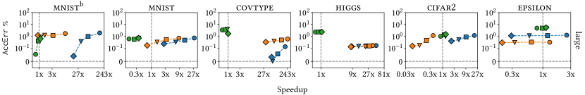
Figure 4. Efficiency-Effectiveness trade-off at $\sigma=1$ for the largest volume of deletion as $\tau$ is varied. The y-axis reports effectiveness (AccErr) and the x-axis reports efficiency (speed-up). The legend is same as in Figure 3.

6.1. Efficiency and Certifiability Trade-Off

In this experiment, we evaluate the trade-off between certifiability and efficiency of each unlearning method when the noise parameter $\sigma$ is kept constant and the efficiency parameter $\tau$ is varied. The efficiency parameter for Fisher and Influence is the size of the unlearning mini-batch $m^{\prime}$ and its values are

$$\tau_{{}_{\textsc{Fisher}}},\tau_{{}_{\textsc{Influence}}}=m^{\prime}\in\left\{m,\left\lfloor\frac{m}{2}\right\rfloor,\left\lfloor\frac{m}{4}\right\rfloor,\left\lfloor\frac{m}{8}\right\rfloor\right\},$$

where $m$ is the volume of deleted data. For the DeltaGrad method the efficiency parameter is the periodicity $T_{0}$ of the unlearning algorithm, and its values are

$$\tau_{{}_{\textsc{DeltaGrad}}}=T_{0}\in\{2,5,50,100\}.$$

We obtain the updated model $\mathbf{w}^{u}$ and the fully retrained model $\mathbf{w}^{*}$ for each unlearning method as described in Sections 3.2, 3.4 and 3.3 at a fixed value of $\sigma$.

The results are shown in Figure 3. We report the results for two fixed values of the noise parameter and specific volumes of deletion. First in Figure 3(a), we fix $\sigma=0$ and present results for all volumes of deletion corresponding to each row in the figure. Second, in Figure 3(b), we fix $\sigma=1$ and present results corresponding only to the largest deletion volume (due to page-limit constraints). For each plot in the figure, the y-axis reports certifiability (AccDis) and the x-axis reports efficiency (speed-up). Different unlearning methods and values of $\tau$ are indicated with different colors and markers respectively in the legend. For extensive results covering different values of $\sigma$ and volumes of deletion, please refer to Appendix C and Table 7

We observe three main trends from Figure 3. First, we observe the general trade-off between efficiency and certifiability: higher efficiency (i.e., higher speedup) is typically associated with lower certifiability (i.e., higher AccDis) in the plots. Some discontinuity in the plotlines, especially for DeltaGrad, is largely due to the convergence criteria, particularly since DeltaGrad employs SGD not only for training but also for unlearning.

Second, the Influence and Fisher methods have a roughly similar trend for each dataset. For the low dimensional datasets they provide large speed-ups of nearly 200x and 50x for each dataset respectively when performing bulk removals (i.e., $m^{\prime}=m$), while DeltaGrad provides speed-up $<1\text{x}$, i.e., requiring more time than the fully retrained model. This is because the cost of computing the inverse Hessian matrix (see Eqs. 6 and 14) for Influence and Fisher, is much lower when dimensionality is low, compared to the cost of approximating a large number of SGD iterations for the DeltaGrad method. Conversely, for the high dimensional datasets, Influence and Fisher provide a smaller speed-up, even when bulk removals are performed (5x and 1.8x respectively for each dataset); and when $\tau$ is decreased to $m^{\prime}=\lfloor m/8\rfloor$, the efficiency is further reduced (1.03x and 0.35x). Whereas DeltaGrad at $T_{0}=50$ provides comparable and better speed-ups of 2.9x and 2.5x respectively, with similar values of AccDis as compared to the other methods.

Third, as the volume of deletions increases (see the rows of Figure 3(a)), the range of AccDis increases as well. This is because as we delete more data points, the updated model $\mathbf{w}^{u}$ diverges from the fully retained model $\mathbf{w}^{*}$ due to the approximations in the unlearning algorithm of each method, leading to higher disparity. This is clearly seen at the largest values of the efficiency parameter ($m^{\prime}=m$ and $T_{0}=100$), where the unlearning algorithm sacrifices the most certifiability, indicated by the largest disparity in accuracy.

Lastly, the trends for DeltaGrad are similar to the previous results at $\sigma=0$. However, the efficiency for the high dimensional datasets is lower, due to the computational cost of noise injection (see Eq. 16). Furthermore, the certifiability has slightly improved for the low dimensional datasets, as indicated by lower values of AccDis, due to the injected noise. We also note that increasing the efficiency parameter offers only minor improvements in speed-up, at much larger values of accuracy disparity.

6.2. Efficiency and Effectiveness Trade-Off

In this experiment, we evaluate how varying the efficiency parameter $\tau$ trades-off efficiency for effectiveness when the volume of data deleted and $\sigma$ are kept constant. The range of $\tau$ for each unlearning method is the same as in Section 6.1. In Figure 4, we discuss the results for $\sigma=1$ and the large volume of deletion for each dataset. For extensive results covering all different values of $\sigma$ and volumes of deletion, please refer to Appendix C and Table 7. In each plot, effectiveness is reported as the test accuracy error AccErr, and efficiency is reported as the speed-up in running time (metrics defined in Section 4.3). We observe the following trends. First, we observe the general trade-off: higher efficiency (i.e., higher speed-up) is typically associated with lower accuracy error (i.e., AccErr) for the same method.

Second, we observe that the Influence offers the best efficiency and effectiveness trade-off among all the methods. Especially, for the high dimensional datasets, the highest efficiency offered is 20x and 2.5x respectively compared to 0.4x and 1.3x of Fisher, at a slightly larger test accuracy error ($1.17\%$ and $1.2\%$ respectively compared to $1.16\%$ and $0.3\%$ of Fisher). For the low dimensional datasets, Influence and Fisher offer similar efficiency and effectiveness. Lastly, for the moderate dimensional datasets, the largest efficiency Influence offers is 168x and 29x respectively compared to 9x and 8.5x of Fisher, at a lower test accuracy error. Furthermore, decreasing the $\tau$ in the unlearning algorithm leads to lower test accuracy error as seen clearly in $\text{\sc mnist}^{\text{b}}$ and covtype datasets, because the noise is injected only in the training algorithm.

Third, we again see that DeltaGrad is mostly stable both in terms of efficiency and effectiveness as seen in Section 6.1. However, note that the test accuracy error for all datasets is larger compared to the other methods due to the direct noise injection (see Eq. 16) and hence offers a lower effectiveness even at $\sigma=1$.

Lastly, Fisher offers much lower efficiency for the high dimensional datasets compared to Section 6.1, where the speed-up is $\leq$1x for nearly all choices of the efficiency parameter.

This is due to the reduced computational effort required to obtain the fully retrained model $\mathbf{w}^{*}$ as no noise injection is done. Therefore, it takes longer to inject noise using the Fisher unlearning algorithm and obtain an updated model compared to obtaining the fully retrained model, especially when dimensionality is high. Also, we see that due to the amount of noise injected in the unlearning algorithm, reducing the efficiency parameter only slightly reduces the test accuracy error of the method.

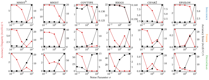
Figure 5. Effectiveness-Certifiability trade-offs for largest volume of deletion. Each row corresponds to an unlearning method. Efficiency parameter is fixed at $m^{\prime}=m$ for Influence and Fisher and $T_{0}=100$ for DeltaGrad. Left y-axis reports certifiability (AccDis), right y-axis reports effectiveness (AccErr) and x-axis varies noise parameter $\sigma$. Lower is better for both y-axes.

6.3. Effectiveness and Certifiability Trade-Off

Figure 6. Effect of noise parameter $\sigma$ on the updated model $\mathbf{w}^{u}$ when no data points are deleted. The first row reports the effectiveness (AccErr) and second row reports the $L_{2}$ distance between $\mathbf{w}^{u}$ and the optimal model

In this section, we first study the effect of the noise parameter $\sigma$ on the effectiveness of a fully trained ML model $\mathbf{w}^{*}$. Next, we evaluate how varying the noise parameter $\sigma$ trades-off effectiveness for certifiability for each unlearning method when the volume of data deleted and the $\tau$ parameter are kept constant.

Effect of $\sigma$ on $\mathbf{w}^{*}$ To isolate the effect of data deletion and for simplicity, we select a deletion fraction of 0, i.e., no data is deleted. We vary $\sigma$ from $10^{-2}$ till $10^{2}$ and obtain a fully trained model $\mathbf{w}^{*}$ using the training algorithm of each unlearning method (see Eqs. 3, 15 and 11) on the initial dataset $\mathcal{D}_{\text{init}}$. Then, we compare this model with the optimal model (a fully trained model with $\sigma=0$) on the initial dataset. The results are presented in Figure 6, where we report in the first row the effectiveness using accuracy error AccErr and in the second row the $L_{2}$ distance between the two models. As no data is deleted, we cannot report the accuracy disparity, hence the $L_{2}$ distance acts a proxy for the disparity between the fully trained model and the optimal model.

In Figure 6, we notice the difference in the extent of the test accuracy error and the $L_{2}$ distance as a consequence of the noise injection in each unlearning method at different values of $\sigma$. First, the Influence method has the smallest AccErr and $L_{2}$ distance from the optimal model – a direct consequence of noise injection in its objective function (see Eq. 10) and the subsequent optimization by the SGD algorithm during the training stage. Second, the DeltaGrad method has the largest AccErr and $L_{2}$ distance from the optimal model, even at small values of $\sigma$, due to random noise directly injected into the model parameters (see Eq. 15). Lastly, the Fisher method sits in-between the other methods, both in terms AccErr and $L_{2}$ distance due to the injection of random noise in the direction of the Fisher matrix (see Eq. 3). This lessens the impact on the model parameters in comparison to the DeltaGrad method, however, the impact is still greater compared to the optimized noise injection in the Influence method.

Trade-off experiments Here we only present the results for the largest deletion volume from Table 2. For more extensive experiments covering different $\tau$ parameters and volumes of deletion, refer Appendices E and 8. The efficiency parameter $\tau$ was set as follows: for Influence and Fisher, we set

$$\tau_{{}_{\textsc{Influence}}}=\tau_{{}_{\textsc{Fisher}}}=m^{\prime}:=m,$$

i.e., the size of the unlearning mini-batch was set to be equal to the volume of deleted data; and for DeltaGrad, we set

$$\tau_{{}_{\textsc{DeltaGrad}}}=T_{0}:=100,$$

i.e., the periodicity is set to 100 SGD steps.

For different values of the noise parameter $\sigma$, we obtain the updated models $\mathbf{w}^{u}$ corresponding to each unlearning method as described in Sections 3.2, 3.4 and 3.3. For baselines, first we obtain the fully retrained model $\mathbf{w}^{*}$ at the same $\sigma$ to measure certifiability and a second fully retrained model $\mathbf{w}^{*}$ at $\sigma=0$ to measure effectiveness, as per Section 4.3. The results are shown in Figure 5. For each plot in the figure, the left y-axis reports the certifiability (AccDis), the right y-axis reports effectiveness (AccErr). as the $\sigma$ is varied from $10^{-2}$ till ${10^{2}}$ for the different unlearning methods.

First, notice that we observe the trade-off between effectiveness and certifiability: higher effectiveness (lower AccErr) is typically associated with lower certifiability (higher AccDis).

Another clear observation is that for Influence method, the test accuracy error AccErr remains low for most of the range of $\sigma$, and increases only at higher values of $\sigma$ ($\geq 10^{1}$). Moreover, we see its largest AccErr is lower than other methods across all datasets. For example, in the mnist dataset, the maximum AccErr (at $\sigma=100$) is approximately $19\%$, $40\%$ and $79\%$ and for Influence, Fisher and DeltaGrad respectively. At the same time, however, improved certifiability (i.e., decreased AccDis) is achieved for high values of $\sigma$. Therefore, to obtain a good combination of effectiveness and efficiency, one must select higher values of $\sigma$, based on the dataset.

Moreover, for Fisher near $\sigma=1$, the trade-off between AccErr and AccDis is the best amongst all methods across all datasets, AccErr is 1.7, 0.7, 0.6, 0.16, 1.15 & 0.7 percent and AccDis is 2.5, 15, 0.1, 0.02, 3 & 0.03 percent for the datasets respectively as seen in Figure 5. If a good effectiveness-certifiability trade-off is required, then the Fisher method appears to be a very suitable method.

Note that, because Influence and Fisher share the same efficiency parameter $\tau$, their experimental results in this section are directly comparable. However, generally that’s not the case with DeltaGrad. As we saw earlier in this section, DeltaGrad is typically quite slower than the other two methods, as evidenced in the achieved speed-ups. Therefore, for these experiments, we invoked it with the largest value of $\tau_{{}_{\textsc{DeltaGrad}}}=T_{0}:=100$, so that its running time is as small as possible and closer to the running time of the other two methods (and, in fact, comparable for the high-dimensional datasets). As discussed in Wu et al. (2020a), the effectiveness of the DeltaGrad method decreases only slightly when the periodicity $T_{0}$ is set to larger values. Therefore, for the same computational budget as the other methods, the trade-off between certifiability and effectiveness for DeltaGrad will be similar to that shown in Figure 5. We can observe this in figs. 19, 22 and 25, where the rows correspond to different $\tau$ parameters for DeltaGrad. We see across the rows for each dataset, the AccErr is similar, while small differences exist in AccDis due to the randomness of the noise injected.

7. When to Retrain

When the updated model $\mathbf{w}^{u}$ is obtained after data deletion (see Figure 1), a decision is made on whether to employ the model for inference – or discard it, restart the pipeline, and train a new model on the remaining data. Specifically, if the test accuracy $\text{\tt Acc}_{\text{test}}$ and certifiability disparity AccDis of the updated model meet certain pre-determined thresholds, then the model is employed for inference, otherwise the pipeline restarts. Notice, though, that measuring AccDis directly as per Eq. 20 would require the fully retrained model $\mathbf{w}^{*}$, which is not readily available. In fact, actually computing $\mathbf{w}^{*}$ after every deletion would defeat the purpose of utilizing an unlearning method in the first place. Moreover, if data deletions occur instantaneously, the current subset of deleted data $\mathcal{D}_{m}$ will not be available for the computation of AccDis (Eq. 20).

Therefore, in practice, AccDis needs to be estimated. We propose an estimate based on the empirical observation that, as more data are deleted, accuracy disparity grows proportionally to how much the test accuracy error in comparison to the initial model.

(22) $$\widetilde{\texttt{AccDis}}=c\cdot\texttt{AccErr}_{\text{init}},$$

where $\widetilde{\texttt{AccDis}}$ is the estimate of AccDis for the updated model, $\texttt{AccErr}_{\text{init}}$ is the test accuracy error relative to the initial model $\mathbf{w}^{*}$,

(23) $$\texttt{AccErr}_{\text{init}}=\text{\tt SAPE}(\text{\tt Acc}_{\text{test}}^{\text{init}},~{}\text{\tt Acc}_{\text{test}}^{u})$$

and $c$ is a constant proportion learned from the data before the pipeline starts. Specifically, $c$ is calculated in three steps. First, after training the model $\mathbf{w}^{*}_{\text{init}}$ on the initial dataset, its test accuracy $\text{\tt Acc}_{\text{test}}^{\text{init}}$ is calculated. Second, an updated model $\mathbf{w}^{u}$ and a fully retrained model $\mathbf{w}^{*}$ is obtained, at the highest value of the efficiency parameter $\tau$, for a sufficiently large deletion fraction $\theta$, say $\theta=0.5$. Third, the proportion $c$ calculated as

$$c=\left[\frac{\texttt{AccDis}}{\texttt{AccErr}_{\text{init}}}\right]_{\text{deletion fraction}=\theta}$$

Table 3. Correlation between $\texttt{AccErr}_{\text{init}}$ and AccDis with targeted-random deletion distribution for the Fisher unlearning method ($m^{\prime}=m$).

Dataset	Pearson Corr.	Spearman Corr.
$\text{\sc mnist}^{\text{b}}$	0.963	0.612
mnist	0.999	1
covtype	0.881	0.964
higgs	0.478	0.892
cifar2	0.938	0.976
epsilon	0.8787	0.891

The empirical measurements in support of this estimate are shown in Table 3, that reports the Pearson and Spearman correlations between AccDis and $\texttt{AccErr}_{\text{init}}$ under a targeted-random deletion distribution and varying the deletion fraction from $0.01$ till $0.45$ ($0.095$ for mnist) utilizing the Fisher unlearning method ($m^{\prime}=m$). From Table 3, we see that apart from the higgs dataset, there is a large and positive correlation between $\texttt{AccErr}_{\text{init}}$ and AccDis, which supports the linear estimate of Eq. 22. The low correlation values of the higgs dataset can be attributed to the issue regarding variance that was observed when using the targeted-random deletion distribution as discussed in Section 5. Now, when an updated model $\mathbf{w}^{u}$ is obtained from the unlearning stage, the $\texttt{AccErr}_{\text{init}}$ is measured using the stored $\text{\tt Acc}_{\text{test}}^{\text{init}}$, and the certifiability disparity is predicted using Equation 22. If the predicted $\widetilde{\texttt{AccDis}}$ exceeds the given threshold for certifiability, then the pipeline restarts and trains a new initial model from scratch on the remaining data and the steps are repeated.

Admittedly, the estimate of Eq. 22 is highly simplistic, but it is also easy to compute, and we have found empirically that it provides conservative estimates (i.e., mild overestimation of the true value) . The mean squared errors (MSE) of the proposed estimator of AccDis for the Fisher unlearning method is shown in Table 4. We observe apart from the higgs and covtype dataset, the errors are low for the proposed estimator. The large error for the higgs data are expected from the discussion above and the low Pearson correlation we observed in Table 3. Similarly, the slightly lower Pearson correlation of the covtype dataset leads to larger MSE when utilizing the simple linear estimator. However, the larger Spearman correlation for the covtype dataset as seen in Table 3, indicates that a non-linear estimator can better capture the relationship between $\texttt{AccErr}_{\text{init}}$ and AccDis. The design of more sophisticated models or algorithms to better estimate the certification disparity is left for future work.

Table 4. Mean Squared Error (MSE) of the proposed estimator of AccDis for the Fisher unlearning method ($m^{\prime}=m$). Proportion $c$ is computed at deletion fraction $\theta=0.45$ using targeted-random deletions.

Dataset	MSE
$\text{\sc mnist}^{\text{b}}$	0.15
mnist	3.249
covtype	427.77
higgs	2445.24
cifar2	47.088
epsilon	35.775

8. Conclusion

We provided an experimental evaluation of three state-of-the-art machine unlearning methods for linear models. We found that, for the right parameterization, Fisher and Influence offer a combination of good performance qualities, at significant speed-up compared to full retraining; and that DeltaGrad offers stable, albeit not as competitive performance. Moreover, we proposed an online strategy to evaluate an updated ML model and determine if it satisfies the requirements of the pipeline and when a full-retraining on the remaining data is required.

Our work falls within a wider research area in which ML tasks (e.g., machine unlearning, in this paper) are studied not only in terms of predictive performance (effectiveness), but also in terms of system efficiency. For future work, several possibilities are open ahead. One direction is to extend the study to general data updates (i.e., not only data deletions) and other ML settings (e.g., to update more complex models, such as neural networks). And another direction is to develop more elaborate mechanisms to determine when a full retraining of the updated models is needed.

Appendix A Experimental Setup

In this section we discuss the additional details regarding the experiments and the implementation of the common ML pipeline.

A.1. Training

Ensuring that the training phase of the common ML pipeline, especially the optimization of each unlearning method is a difficult task. As mentioned in Section 4.2, Influence and Fisher require SGD convergence and DeltaGrad can only use vanilla SGD. The additional constraints come from the DeltaGrad method. Wu et al. (2020a) describes that smaller mini-batch size leads to lower approximation and hence lower effectiveness. However, choosing a full-batch gradient descent update as described in Equation 2 to ensure best performance of the DeltaGrad method leads to the requirement of a large number of epochs to achieve converge for Influence and Fisher. This is computationally expensive both in calculation of full-batch gradients for the large datasets such as epsilon and higgs and the number of epochs required in total to reach convergence. Ideally to reduce the impact of the latter, we would fix a number of epochs and then select a larger learning rate $\eta$ to compensate for the slower average gradient updates. However, we experimentally found that increasing the learning rate $\eta$ beyond 1 has a significant impact on the performance of DeltaGrad. This is primarily because the error in the approximate SGD step is amplified as the learning rate is increased beyond the optimal learning rate (which results in an increased number of epochs to achieve the same convergence). These constraints and limitations led us to fix the learning rate to 1 and choose large enough mini-batches (for DeltaGrad performance) while keeping the number of epochs low (for computational effort) using a small validation dataset of the initial training data $\mathcal{D}_{\text{init}}$. The chosen values of the mini-batch size and the number of epochs for each dataset is described in Table 5.

Table 5. Values of training parameters common for all unlearning methods

Dataset	epochs	mini-batch size
$\text{\sc mnist}^{\text{b}}$	1000	1024
mnist	200	512
covtype	200	512
higgs	20	512
cifar2	500	512
epsilon	60	512

A.2. DeltaGrad unlearning method

As described in Section 3.4, the primary $\tau$ parameter chosen for the DeltaGrad method was the periodicity $T_{0}$. Based on the discussion of the hyper-parameter of the DeltaGrad in Wu et al. (2020a), the ideal $\tau$ parameter would be the training mini-batch size. However, this would result in a non-standard training stage in the ML pipeline for the DeltaGrad which in turn prevents any comparison with the other unlearning methods. Therefore, upon fixing the common training stage, we choose the hyper-parameter $T_{0}$ that best represents the trade-off between effectiveness and efficiency. The remaining candidate $\tau$ parameters are the burn-in period $j_{0}$ and the size of the history for the L-BFGS algorithm $h$. Following Wu et al. (2020a), we fix $h=2$ for all datasets and the values of $j_{0}$ are presented in Table 6.

Table 6. Values of DeltaGrad burn-in period parameter $j_{0}$.

Dataset	$j_{0}$
$\text{\sc mnist}^{\text{b}}$	10
mnist	20
covtype	10
higgs	500
cifar2	20
epsilon	10

Appendix B Extended Deletion Distribution Results

In Figure 7, we present the extended results for the uniform-random and uniform-informed deletion distribution. We increase the fraction of data deleted from $0.5$ till $0.995$. We see that the drop in both $\text{\tt Acc}_{\text{test}}$ and $\text{\tt Acc}_{\text{del}}$ only occur when we delete beyond $90\%$ of the initial training data. We also clearly see that the drop in both metric is much steeper for the uniform-informed distribution compared to the uniform-random distribution. This indicates that the informed deletions are deleting outliers that are required by the ML model to effectively classify samples.

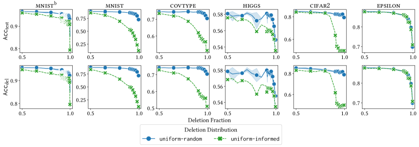
Figure 7. Extended deletion distribution results. Deletion fraction varied from $0.5$ till $0.995$. Only uniform-random and uniform-informed deletion distribution results are reported.

Appendix C Certifiability-Efficiency Trade-off results

In this section, we present the additional results of the trade-off between certifiability and efficiency as the $\tau$ parameter is varied at different volumes of deletion and values of $\sigma$. In Table 8, we provide an interface to easily navigate to the results corresponding to each value of $\sigma$. In each figure, there are sub-figures corresponding to different volumes of deletion. For example, Figure 8 presents results for when $\sigma=0.01$ and sub-figures figs. 8(a), 8(b) and 8(c) correspond to the small, medium and large deletion volumes described in Table 2. The legend for the range of the $\tau$ parameter is the same as that found in Figure 3.

There are two interesting trends to note from these results. First, is that for values of $\sigma<1$, we see little to no difference in the trend of the trade-off offered. This is due to the smaller quantities of injected noise that does not increase certifiability by reducing the accuracy disparity. Second, is that for smaller volumes of deletion, all of the unlearning methods have lower AccDis and offer higher certifiability, especially at lower values of $\tau$. This is because the unlearning algorithms of each method are better able approximate the fully-retrained model as the number of deleted points is fewer.

Table 7. Links to results for the trade-offs for efficiency.

Trade-Off	$\sigma$
	0.01	0.1	1	10	100
Certifiability-Efficiency	fig. 8	fig. 9	fig. 10	fig. 11	fig. 12
Effectiveness-Efficiency	fig. 13	fig. 14	fig. 15	fig. 16	fig. 17

(a) small deletion fraction

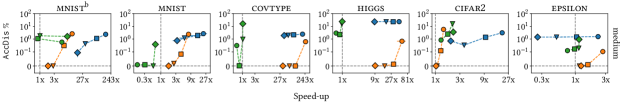
(b) medium deletion fraction

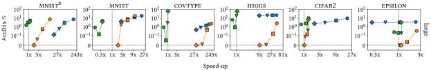
(c) large deletion fraction

Figure 8. Certifiability and efficiency trade-off results for $\sigma=0.01$ at different volumes of deletion : (a) small (b) medium and (c) large. AccDis is reported on the y-axis and the speed-up in running time on the x-axis. Legend is same as in fig. 3

(a) small deletion fraction

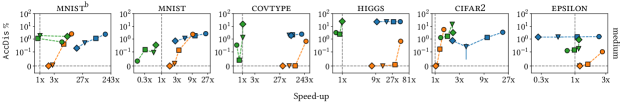
(b) medium deletion fraction

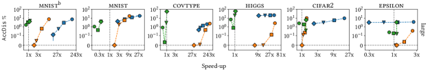
(c) large deletion fraction

Figure 9. Certifiability and efficiency trade-off results for $\sigma=0.1$ at different volumes of deletion : (a) small (b) medium and (c) large. AccDis is reported on the y-axis and the speed-up in running time on the x-axis. Legend is same as in fig. 3

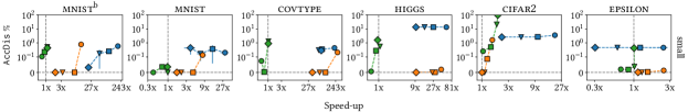
(a) small deletion fraction

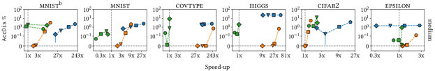
(b) medium deletion fraction

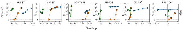
(c) large deletion fraction

Figure 10. Certifiability and efficiency trade-off results for $\sigma=1$ at different volumes of deletion : (a) small (b) medium and (c) large. AccDis is reported on the y-axis and the speed-up in running time on the x-axis. Legend is same as in fig. 3

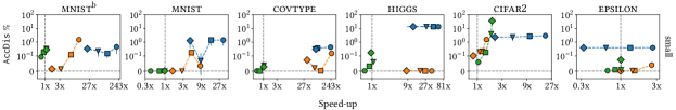
(a) small deletion fraction

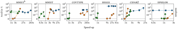
(b) medium deletion fraction

(c) large deletion fraction

Figure 11. Certifiability and efficiency trade-off results for $\sigma=10$ at different volumes of deletion : (a) small (b) medium and (c) large. AccDis is reported on the y-axis and the speed-up in running time on the x-axis. Legend is same as in fig. 3

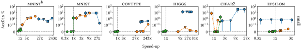
(a) small deletion fraction

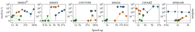
(b) medium deletion fraction

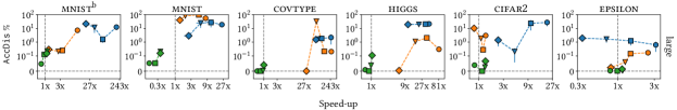
(c) large deletion fraction

Figure 12. Certifiability and efficiency trade-off results for $\sigma=100$ at different volumes of deletion : (a) small (b) medium and (c) large. AccDis is reported on the y-axis and the speed-up in running time on the x-axis. Legend is same as in fig. 3

Appendix D Effectiveness-Efficiency Trade-off Results

In this section, we present the additional results of the trade-off between efficiency and effectiveness as the $\tau$ parameter is varied for different volumes of deletion and values of $\sigma$. In Table 8, we provide an interface to easily navigate to the results corresponding to each value of $\sigma$. In each figure, there are sub-figures corresponding to different volumes of deletion. For example, Figure 13 presents results for when $\sigma=0.01$ and sub-figures figs. 13(a), 13(b) and 13(c) correspond to the small, medium and large deletion volumes described in Table 2. The legend for the range of the $\tau$ parameter is the same as that found in Figure 3.

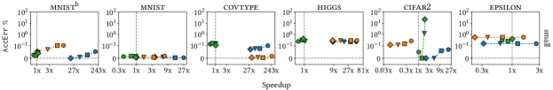
(a) small deletion fraction

(b) medium deletion fraction

(c) large deletion fraction

Figure 13. Effectiveness and efficiency trade-off results for $\sigma=0.01$ at different volumes of deletion : (a) small (b) medium and (c) large. AccErr is reported on the y-axis and the speed-up in running time on the x-axis. Legend is same as in fig. 3

(a) small deletion fraction

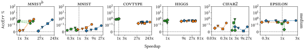
(b) medium deletion fraction

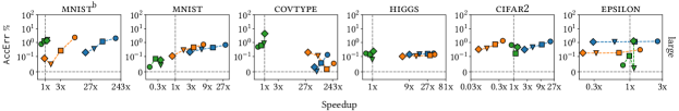
(c) large deletion fraction

Figure 14. Effectiveness and efficiency trade-off results for $\sigma=0.1$ at different volumes of deletion : (a) small (b) medium and (c) large. AccErr is reported on the y-axis and the speed-up in running time on the x-axis. Legend is same as in fig. 3

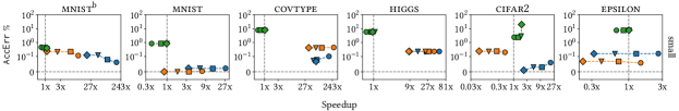
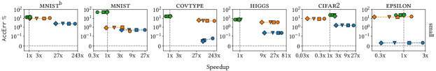
(a) small deletion fraction

(b) medium deletion fraction

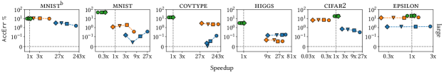
(c) large deletion fraction

Figure 15. Effectiveness and efficiency trade-off results for $\sigma=1$ at different volumes of deletion : (a) small (b) medium and (c) large. AccErr is reported on the y-axis and the speed-up in running time on the x-axis. Legend is same as in fig. 3

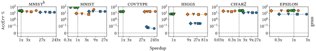
(a) small deletion fraction

(b) medium deletion fraction

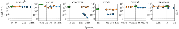
(c) large deletion fraction

Figure 16. Effectiveness and efficiency trade-off results for $\sigma=10$ at different volumes of deletion : (a) small (b) medium and (c) large. AccErr is reported on the y-axis and the speed-up in running time on the x-axis. Legend is same as in fig. 3

(a) small deletion fraction

(b) medium deletion fraction

(c) large deletion fraction

Figure 17. Effectiveness and efficiency trade-off results for $\sigma=100$ at different volumes of deletion : (a) small (b) medium and (c) large. AccErr is reported on the y-axis and the speed-up in running time on the x-axis. Legend is same as in fig. 3

Appendix E Certifiability-Effectiveness Trade-off Results

In this section, we present the additional results for the trade-off between certifiability and effectiveness as $\sigma$ is varied for different volumes of deletions and values of the $\tau$ parameter. In Sections E.1, E.2 and E.3 we present the results corresponding to the small, medium and large deletion volumes described in Table 2. In each subsection, we present the results for each unlearning method in a figure, where the rows of the figure correspond to different values of the $\tau$ parameter. In Table 8, we provide an interface to easily navigate to the results corresponding to each unlearning method and volume of deletion.

Table 8. Links to results of the trade-off between certifiability and effectiveness for different methods and deletion volumes

Method	Deletion Volume
	small	medium	large
Fisher	fig. 18	fig. 21	fig. 24
DeltaGrad	fig. 19	fig. 22	fig. 25
Influence	fig. 20	fig. 20	fig. 20

E.1. Small deletion volume results

In this subsection, Figures 18, 19 and 20 correspond to the results for the Fisher, DeltaGrad and Influence methods for the smallest volume of deleted data.

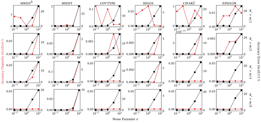
Figure 18. Certifiability-Effectiveness trade-off for Fisher method at small deletion volume. Each row corresponds to a value of the $\tau$ parameter

Figure 19. Certifiability-Effectiveness trade-off for DeltaGrad method at small deletion volume. Each row corresponds to a value of the $\tau$ parameter

Figure 20. Certifiability-Effectiveness trade-off for Influence method at small deletion volume. Each row corresponds to a value of the $\tau$ parameter

E.2. Medium deletion volume results

In this subsection, Figures 21, 22 and 23 correspond to the results for the Fisher, DeltaGrad and Influence methods for the medium volume of deleted data.

Figure 21. Certifiability-Effectiveness trade-off for Fisher method at medium deletion volume. Each row corresponds to a value of the $\tau$ parameter

Figure 22. Certifiability-Effectiveness trade-off for DeltaGrad method at medium deletion volume. Each row corresponds to a value of the $\tau$ parameter

Figure 23. Certifiability-Effectiveness trade-off for Influence method at medium deletion volume. Each row corresponds to a value of the $\tau$ parameter

E.3. Large deletion volume results

In this subsection, Figures 24, 25 and 26 correspond to the results for the Fisher, DeltaGrad and Influence methods for the largest volume of deleted data.

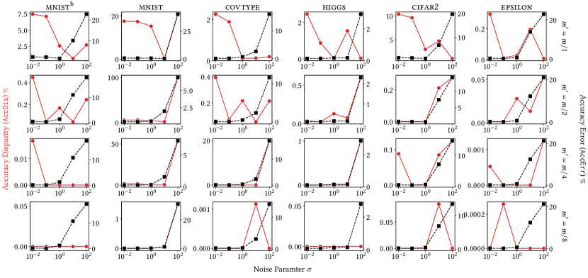
Figure 24. Certifiability-Effectiveness trade-off for Fisher method at large deletion volume. Each row corresponds to a value of the $\tau$ parameter

Figure 25. Certifiability-Effectiveness trade-off for DeltaGrad method at large deletion volume. Each row corresponds to a value of the $\tau$ parameter

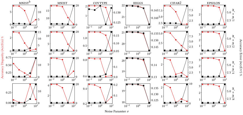
Figure 26. Certifiability-Effectiveness trade-off for Influence method at large deletion volume. Each row corresponds to a value of the $\tau$ parameter

References

- (1)
- Baldi et al. (2014) P. Baldi, P. Sadowski, and D. Whiteson. 2014. Searching for exotic particles in high-energy physics with deep learning. Nature Communications 5, 1 (Jul 2014). https://doi.org/10.1038/ncomms5308
- Bourtoule et al. (2020) Lucas Bourtoule, Varun Chandrasekaran, Christopher A. Choquette-Choo, Hengrui Jia, Adelin Travers, Baiwu Zhang, David Lie, and Nicolas Papernot. 2020. Machine Unlearning. arXiv:1912.03817 [cs] (July 2020). arXiv:1912.03817 [cs]
- Boyd et al. (2004) Stephen Boyd, Stephen P Boyd, and Lieven Vandenberghe. 2004. Convex optimization. Cambridge university press.
- Brophy and Lowd (2021) Jonathan Brophy and Daniel Lowd. 2021. Machine Unlearning for Random Forests. (2021). arXiv:2009.05567 [cs.LG]
- Cao and Yang (2015) Yinzhi Cao and Junfeng Yang. 2015. Towards Making Systems Forget with Machine Unlearning. In 2015 IEEE Symposium on Security and Privacy. IEEE, San Jose, CA, 463–480. https://doi.org/10.1109/SP.2015.35
- Chang and Lin (2011) Chih-Chung Chang and Chih-Jen Lin. 2011. LIBSVM: A library for support vector machines. ACM Transactions on Intelligent Systems and Technology 2 (2011), 27:1–27:27. Issue 3. Software available at http://www.csie.ntu.edu.tw/~cjlin/libsvm.
- Chaudhuri and Monteleoni (2009) Kamalika Chaudhuri and Claire Monteleoni. 2009. Privacy-preserving logistic regression. In Advances in Neural Information Processing Systems, D. Koller, D. Schuurmans, Y. Bengio, and L. Bottou (Eds.), Vol. 21. Curran Associates, Inc. https://proceedings.neurips.cc/paper/2008/file/8065d07da4a77621450aa84fee5656d9-Paper.pdf
- Collobert et al. (2002) Ronan Collobert, Samy Bengio, and Yoshua Bengio. 2002. A Parallel Mixture of SVMs for Very Large Scale Problems. Neural Comput. 14, 5 (May 2002), 1105–1114. https://doi.org/10.1162/089976602753633402
- Dwork et al. (2014) Cynthia Dwork, Aaron Roth, et al. 2014. The algorithmic foundations of differential privacy. Foundations and Trends in Theoretical Computer Science 9, 3-4 (2014), 211–407.
- Golatkar et al. (2020c) Aditya Golatkar, Alessandro Achille, Avinash Ravichandran, Marzia Polito, and Stefano Soatto. 2020c. Mixed-Privacy Forgetting in Deep Networks. arXiv:2012.13431 [cs] (Dec. 2020). arXiv:2012.13431 [cs]
- Golatkar et al. (2020a) Aditya Golatkar, Alessandro Achille, and Stefano Soatto. 2020a. Eternal Sunshine of the Spotless Net: Selective Forgetting in Deep Networks. arXiv:1911.04933 [cs, stat] (March 2020). arXiv:1911.04933 [cs, stat]
- Golatkar et al. (2020b) Aditya Golatkar, Alessandro Achille, and Stefano Soatto. 2020b. Forgetting Outside the Box: Scrubbing Deep Networks of Information Accessible from Input-Output Observations. arXiv:2003.02960 [cs, math, stat] (Oct. 2020). arXiv:2003.02960 [cs, math, stat]
- Graves et al. (2020) Laura Graves, Vineel Nagisetty, and Vijay Ganesh. 2020. Amnesiac Machine Learning. arXiv:2010.10981 [cs] (Oct. 2020). arXiv:2010.10981 [cs]
- Guo et al. (2020) Chuan Guo, Tom Goldstein, Awni Hannun, and Laurens van der Maaten. 2020. Certified Data Removal from Machine Learning Models. arXiv:1911.03030 [cs, stat] (Aug. 2020). arXiv:1911.03030 [cs, stat]
- Izzo et al. (2021) Zachary Izzo, Mary Anne Smart, Kamalika Chaudhuri, and James Zou. 2021. Approximate Data Deletion from Machine Learning Models. In Proceedings of The 24th International Conference on Artificial Intelligence and Statistics (Proceedings of Machine Learning Research), Arindam Banerjee and Kenji Fukumizu (Eds.), Vol. 130. PMLR, 2008–2016. http://proceedings.mlr.press/v130/izzo21a.html
- Karasuyama and Takeuchi (2010) M. Karasuyama and I. Takeuchi. 2010. Multiple Incremental Decremental Learning of Support Vector Machines. IEEE Transactions on Neural Networks 21, 7 (2010), 1048–1059. https://doi.org/10.1109/TNN.2010.2048039
- Kingma and Ba (2015) Diederik P. Kingma and Jimmy Ba. 2015. Adam: A Method for Stochastic Optimization. In 3rd International Conference on Learning Representations, ICLR 2015, San Diego, CA, USA, May 7-9, 2015, Conference Track Proceedings, Yoshua Bengio and Yann LeCun (Eds.). http://arxiv.org/abs/1412.6980
- Koh and Liang (2017) Pang Wei Koh and Percy Liang. 2017. Understanding Black-Box Predictions via Influence Functions. arXiv:1703.04730 [cs, stat] (July 2017). arXiv:1703.04730 [cs, stat]
- Krizhevsky et al. ([n.d.]) Alex Krizhevsky, Vinod Nair, and Geoffrey Hinton. [n.d.]. CIFAR-10 (Canadian Institute for Advanced Research). ([n. d.]). http://www.cs.toronto.edu/~kriz/cifar.html
- LeCun and Cortes (2010) Yann LeCun and Corinna Cortes. 2010. MNIST handwritten digit database. http://yann.lecun.com/exdb/mnist/. (2010). http://yann.lecun.com/exdb/mnist/
- Mahadevan and Mathioudakis (2021) Ananth Mahadevan and Michael Mathioudakis. 2021. Certifiable Machine Unlearning for Linear Models. arXiv:2106.15093 [cs.LG]
- Mantelero (2013) Alessandro Mantelero. 2013. The EU Proposal for a General Data Protection Regulation and the roots of the “right to be forgotten”. Computer Law & Security Review 29, 3 (2013), 229–235. https://doi.org/10.1016/j.clsr.2013.03.010
- Martens (2020) James Martens. 2020. New Insights and Perspectives on the Natural Gradient Method. Journal of Machine Learning Research 21, 146 (2020), 1–76. http://jmlr.org/papers/v21/17-678.html
- Neel et al. (2020) Seth Neel, Aaron Roth, and Saeed Sharifi-Malvajerdi. 2020. Descent-to-Delete: Gradient-Based Methods for Machine Unlearning. arXiv:2007.02923 [cs, stat] (July 2020). arXiv:2007.02923 [cs, stat]
- Nguyen et al. ([n.d.]) Quoc Phong Nguyen, Bryan Kian Hsiang Low, and Patrick Jaillet. [n.d.]. Variational Bayesian Unlearning. ([n. d.]), 12.
- of European Union (2016) Council of European Union. 2016. Regulation (EU) 2016/679. https://eur-lex.europa.eu/legal-content/EN/TXT/?uri=CELEX%3A02016R0679-20160504
- Paszke et al. (2019) Adam Paszke, Sam Gross, Francisco Massa, Adam Lerer, James Bradbury, Gregory Chanan, Trevor Killeen, Zeming Lin, Natalia Gimelshein, Luca Antiga, Alban Desmaison, Andreas Kopf, Edward Yang, Zachary DeVito, Martin Raison, Alykhan Tejani, Sasank Chilamkurthy, Benoit Steiner, Lu Fang, Junjie Bai, and Soumith Chintala. 2019. PyTorch: An Imperative Style, High-Performance Deep Learning Library. In Advances in Neural Information Processing Systems 32, H. Wallach, H. Larochelle, A. Beygelzimer, F. d'Alché-Buc, E. Fox, and R. Garnett (Eds.). Curran Associates, Inc., 8024–8035. http://papers.neurips.cc/paper/9015-pytorch-an-imperative-style-high-performance-deep-learning-library.pdf
- Poggio (2000) Tomaso A Poggio. 2000. Incremental and Decremental Support Vector Machine Learning. In NIPS.
- Schelter (2020) Sebastian Schelter. 2020. “Amnesia” – Towards Machine Learning Models That Can Forget User Data Very Fast. In Conference on Innovative Data Systems Research (CIDR). 4.
- Tsai et al. (2014) Cheng-Hao Tsai, Chieh-Yen Lin, and Chih-Jen Lin. 2014. Incremental and Decremental Training for Linear Classification. In Proceedings of the 20th ACM SIGKDD International Conference on Knowledge Discovery and Data Mining (KDD ’14). Association for Computing Machinery, New York, New York, USA, 343–352. https://doi.org/10.1145/2623330.2623661
- Tsoumakas et al. (2008) G. Tsoumakas, I. Katakis, and I. Vlahavas. 2008. Effective and Efficient Multilabel Classification in Domains with Large Number of Labels. (2008).
- Wu et al. (2020a) Yinjun Wu, Edgar Dobriban, and Susan B. Davidson. 2020a. DeltaGrad: Rapid Retraining of Machine Learning Models. arXiv:2006.14755 [cs, stat] (June 2020). arXiv:2006.14755 [cs, stat]
- Wu et al. (2020b) Yinjun Wu, Val Tannen, and Susan B. Davidson. 2020b. PrIU: A Provenance-Based Approach for Incrementally Updating Regression Models. In Proceedings of the 2020 ACM SIGMOD International Conference on Management of Data. ACM, Portland OR USA, 447–462. https://doi.org/10.1145/3318464.3380571