Emerging SYK physics in polaron system

The polaron is treated as a long-lived quasiparticle with slow momenta and current relaxation in Fermi liquid phase. While in this paper, we discuss the possible realization of SYK physics in a polaron system in non-Fermi liquid phase. We reveal the relation between UV cutoff of polaronic momentum $\Lambda_{q}$ and its SYK behavior. The SYK behavior of a polaron system has rarely been investigated before, and the relation between the scattering momentum and the SYK physics has not yet been explored before (to best of our knowledge). We found that the cutoff $\Lambda_{q}$ directly related to the distribution and statistical variance of polaronic coupling term, which becomes Gaussian variable (or Chi-square variable) in SYK limit (i.e., with a large step number of a fractional distance $\Lambda_{q}^{-1}\rightarrow\infty$). Also, we show that the different $\Lambda_{q}^{-1}$ lending support to different phases, including non-Fermi liquid phase and (disordered) Fermi liquid phase, which correspond to ill-defined and well-defined polarons, respectively. The case of pair condensation induced by local coupling, which happen at critical temperature, is also discussed in this paper, which we found that it would suppresses the SYK non-fermi liquid or not, depending on whether the on-site coupling is constant or variant. We deduce the free energy density and the divergent behaviors of anomalous propagator in this case. Finally, we also present a discussion of ensembles of level statistic that depending on which symmetry class the system belongs to, and that can be controlled by the type of disorder.

1 Introduction

The SYK physics emerges usually in the non-Fermi liquid phase with SYK coupling much larger than the fermionic frequency while the fermionic frequency much larger than the coherence scala (incoherent critical metal phase). In such a regime, the quantum critical behaviors can be found in itinerant electron system due to the quantum fluctuation induced quantum phase transition between disordered state (like the gapped symmetry-broken state or gapless thermal insulator) and the Fermi liquid state.

In conformal limit (without the time derivative term in Hamiltonian), there is a U(1) global symmetry in nonperturbed SYK mode. When there is a spontaneous symmetry breaking due to the finite expectation $\langle b\rangle$, where $b$ is the boson operator induced by the charge or spin fluctuation, the many-body spectrum is gapped out but may accompanied by a gapless Goldstone mode due to the preserved (subsystem) symmetries (if any), which is stable against to the phase fluctuation of corresponding order parameter. The U(1) gauge symmetry of $H_{\flat=4}$ term with four-fermion interaction will be broken by the hopping term which lacks its hermitian conjugate. While for the two-SYK mode interacting system, the $U(1)\times U(1)$ can be preserved as long as the hopping term ($\langle b\rangle$) does not contribute to the inter-SYK mode transition (e.g., in the SU(2) symmetries case), and thus the $H_{\flat=4}$ term is unstable against the perturbation of bilinear term.

Different to the standard SYK coupling which is nonlocal and dense, the polaron coupling is constant and short-ranged and thus the many-body effect is perturbative. While the SYK mode has an nonperturbative many-body effect in Wigner-Dyson random matrix esemble, which can not be fully captured by two-point correlation (single-particle function), and thus the functional-derivative approach[10] wound not be useful here, due to the randomness of SYK coupling and disorders. However, we will see that, after considering the normally distributed interactions among fermion indices and momenta, the polaronic coupling which is considered to be short-ranged (and even approximately the contact type) can still be able to creates the spectrum similar to the one with short-range spectral correlation of SYK model [11], and also, the polaronic coupling decays exponentially with real space distance (or approximately decays exponentially with bandwidth or coherence scale in momentum space), which is similar to the exponentially decay of SYK mode self-energy in long-time limit (low-energy boson excitation) with charging process. That reveals the possibility to realize in SYK physics in polaron system. The SYK physics may emerges in polaron system in the range $U/N\ll\omega_{c}\ll\omega\ll g_{q}\ll N$ of frequency space, where $\omega_{c}=W^{2}/g_{q}$ is coherence scala with spectrum bandwidth $W$. Such a limit can be obtained in real space by replacing the frequency with lattice spacing as given in Ref.[13, 23].

We know that the formation of polaron relies on the mobility of impurity within a bath, i.e., the impurities and the majority particles are coherent and contribute to finite bandwidth of the polaron spectrum. While the SYK term exhibits incoherent non-Fermi liquid features expecially in the gapless critical metal phase where the stable mode (boson excitation insteads of quasiparticle) can remains gapless even without turnning to the quantum critical point (and thus without the condensation) due to the preserved symmetries, and thus contributes to the many-body chaotic spectrum. Since the polaron is a kind of quasiparticle or excitation which can exists in both the fermi liquid[1] and non-fermi liquid states. In fermi liquid system, the polaron can be detected as a coherence peak emerges in a broad incoherent background of fermi sea, and the zero momentum polaron becomes stable and long-lived quasiparticle at zero-temperature limit. As the temperature increases, it may be decayed into particle-hole excitations. Even a Cooper-like polaronic pair can exist in polaronic Fermi liquid of many-body system when it satisfies $g\leq W<\omega$ ($g$ is the polaronic coupling, $W$ is the polaron bandwidth, $\omega$ is the fermionic frequency). That is to say, the superconducting ordering is possible to exists in polaronic Fermi liquid in the weak-interacting and high frequency (UV) limit. For polaron as a quasiparticle in fermi liquid state, it will has well-define momenta and can be described by the purely local description in momentum space. That makes it roubust against the short-range perturbations, like the Coulomb repulsive interaction and the short-range hopping. While the SYK mode emerges in the range $g\gg\omega\gg W^{2}/g$, which requires strong interaction, and thus can be extended to zero temperature as the bandwidth is finite. The emergence of incoherent spectral function in a local form signals the appearance of SYK mode. Similar to the polaron, the SYK model can be described purely in the orbital space, instead of real space, as it mostly being studied in zero-dimensional system (although it can be extended to higher spacial dimension[2]) thus the strong SYK interaction could be long-range and nonlocal, which can efficiently breaks the long-range entanglement of fermi-liquid. So what will happen when the polaronic coupling becomes Gaussian distributed in a mang-body system, and being turned to the range that satisfy the SYK requirement? In this paper, we adopt a orbital space$+$ one-dimensional momentum space description to describe this system, where we try to understand the connection and competition effect between polaronic physics and the SYK physics. We found that the emergence of SYK physics require small enough momentum $q$, which corresponds to to $\Lambda_{q}^{-1}$ much larger than the fermion number $N$. Due to the small one-dimensional polaronic momentum $q$, the SYK model can be approximately as 1+1-dimensonal model (we do not consider the many-body localizaion case in the bulk here). By the small $q$ is essential to leads to strong polaronic coupling and the infinite steps for a fractional distance from $q=0$ to $q=\Lambda_{q}$, which is totally $\Lambda_{q}^{-1}$. This is different to the simple $0+1$ space-time dimensional SYK models where the disorder average is over the consecutive integer values of fermion indices, Besides, the small momentum leads to the delocalization in real space, i.e., the nonlocal SYK interaction can further suppresses the fermi liquid. This is similar to the effect of long-range (weakly screened when close to half-filling) Coulomb interaction, which can turn the fermi liquid to non-Fermi liquid. In the mean time, the robustness of polaron in fermi-liquid to the short range hopping as well as the bilinear chemical potential term may help to stablizing the emergent SYK mode, before the long-range entangment of fermi-liquid is completely destroyed by SYK coupling.

In the presence of pair condensation, it usually competes with the SYK non-fermi liquid phase, with the coherence appears as long as the pairing order parameter is nonzero, and for temperature lower than the critical one. We apply sereval ways to deal with this problem to figure out its effects to the SYK physics in many-body system. Novelly, we found that, in the presence of random local field, insteads of many-local field, the constant local coupling term can be formulated to be a $H_{\flat=4}$ non-fermi liquid term, and even the $H_{\flat=2}$ disordered-fermi liquid term, depending on the scaling dimensional of the auxiliary boson field. And the boson field can even has a negative scaling dimension, e.g., in a random-bonded model[29]. Note that for many-body localized state, the ratios of adjacent level spacings follows the Poisson level statistic, while that in random local field state follows the Wigner-Dyson level statistic according to eigenstate thermalization hypothesis[27]. Recently, it has been experimentally proved that[28], the random local field has the same effect with the disorders which is essential for the emergence of SYK physics, e.g., the random local field and the bond-disorder due to the random distribution of ions contribute together to stabilize the quantum spin liquid in Sr₂CuTe_0.5W_0.5O₆. Such disorder could also be the irregular boundary of two-dimensional lattice (with the chiral system being preserved)[25]. Another type of bond disorder could be the vacancies in two-dimensional materials[34]. The preserved symmetries can help to stabilize the SYK physics against the perturbations, and in this paper, there are at least two kinds of symmetries, the SU(2) symmetry, regarding to the spin component of the interacting fermions, and the U(1) gauge symmetry with the charge-conserving interaction. Specifically, in the presence of random local field with defined Gaussian variables $\Phi_{i}$ and $\Phi^{q}$ (wave functions about the fermion index and polaronic momentum, respectively), the thermalization and localization can happen in the mean time to a single fermion, which is different to the case described in Ref.[27]. And in this case, the fermions can be localized by the on-site interaction and thermalized due to the vanishing level spacing, by virtue of random on-site potential.

Once the anomalous components emerge, i.e., the pairing order parameter is nonzero, the level statistic should change from Gaussian unitary ensemble (GUE) to Gaussian orthogonal ensemble (GOE), where GOE has a level repulsion larger than that of GUE in the small level spacing limit during the level statistic. Both the GUE and GOE follow the Wigner-Dyson distribution. However, when the pair condensation happen, in which case the system changes from the volume law phase (with eigenstate thermalization hypothesis) where the entanglement entropy scales linearly with the bipartition size, to the area law phase where the entanglement entropy scales independent of the bipartition size and with short range entanglement[30]. This phase transition can be realized by a many-localized field with strong disorder which can induces random but short-ranged and sparse interactions[27],, or a random quantum circuit with local measurement[32]. Note that here the pair condensation has similar effect with the product of two bilinear term in the unthermalized SYK system[31]. In the extreme case where the eigenvalue splitting is being maximized, the off-diagonal long-range order emerges.

Our main conclusion is that, the SYK physics can be realized in the small polaronic mmentum $\Lambda_{q}$ limit, which is much smaller than the randomly distributed interactions, and in the mean time, the polaron can exists. But once $\Lambda_{q}=0$, the system reduces to the product of two $SYK_{q=2}$ modes due to the flat non-fermi-liquid spectral function. Note that, although the tradictional SYK physics require the system to be momentum-independent, i.e., in zero-dimensional space, which can be experimentally realized under strong magnetic field[25] or in a Kagome-type optical lattice[35] to obtain the flat levels, we here provide a route to realize the SYK physics without completely removing the momentum-dependence, but transform the momentum-dependence to the fermion index-dependence with a certain constrain. We will discuss in detail about this constrain and to what extent this model can realize the SYK physics in this paper.

2 Electronic properties of polaron and related momentum-dependent dynamics

2.1 Self-energy and polariztion function

Firstly we discuss the electronic properties of polaron and the role played by polaronic momentum $q$ during the scattering. When the formation of polaron[3] does not contains the component which has a macroscopic amount, like the phonons or photons (in a cavity), the total momentum of the weakly-coupled propagating pair is conservative, and thus the transport relaxation time of polaron reads $1/\tau\sim\Sigma^{(1)}=ng_{b}$ where $\Sigma^{(1)}$ is the first order contribution to self-energy. $g_{b}$ is the bare coupling strength which equals to the vacuum scattering matrix. For temperature higher than the critical one ($T_{c}=W^{2}/g_{b}$ with $W$ the bandwidth) the non-Fermi-liquid feature, which is hidden by the instability at low temperature, will leads to incoherence between the electronic excitations. Note that the finite-temperature also affects the resonance structure of the polaron spectrum[8]. Besides, the strong coupling in strongly correlated metals will largely reduce the critical temperature, and thus lead to the coherence-to-incoherence crossover, which also happen in the Dirac/Weyl semimetallic states.

By writting the isotropic dispersions of impurity (with spin $\sigma$) and majority (with spin $\sigma^{\prime}$) particles as (before collision) $\varepsilon_{p\sigma}=p^{\alpha}$ and $\varepsilon_{k\sigma^{\prime}}=k^{\beta}$, respectively, the Green's function in Fermi-liquid phase are $G_{p\sigma}^{-1}=iZ^{-1}\omega-\varepsilon_{p\sigma}$ and $G_{q\sigma^{\prime}}^{-1}=iZ^{-1}\Omega-\varepsilon_{q\sigma^{\prime}}$, respectively, where $Z=1-(g_{q}D_{0})^{2}$ is the quasiparticle residue in weak-coupling limit[4], and we define $g_{q}$ as the polaronic coupling and $D_{0}$ as the bare density-of-states. The Chevy-type variational ansatz for a mobile impurity with momentum $p$ dressed by one electron-hole pairs (excitations) is

$$|\psi\rangle=\psi_{0}b^{{\dagger}}_{p\sigma}|0\rangle_{\sigma^{\prime}}+\sum_{q}\psi_{kq}c_{p+q-k,\sigma}^{{\dagger}}c_{k,\sigma^{\prime}}^{{\dagger}}|0\rangle_{\sigma^{\prime}},$$ (1)

where $|0\rangle_{\sigma^{\prime}}=\Pi_{k<k_{F}}c_{k\sigma^{\prime}}^{{\dagger}}|{\rm vac}\rangle$ is the ground state of majority particles. $c^{{\dagger}}_{k\sigma^{\prime}}$ is the creation operator of the excited particle with momentum $k$, and $c_{q\sigma^{\prime}}$ is the the annihilation operator of the hole at momentum $q$. Here $k>k_{F}$ is to make sure the particles are excited out of the Fermi surface.

We write the polaron Hamiltonian in a continuum model as

$$H=\sum_{p}\varepsilon_{p\sigma}c^{{\dagger}}_{p}c_{p}+\sum_{k}\varepsilon_{k\sigma^{\prime}}c^{{\dagger}}_{k}c_{k}+\sum_{k,p,q}g_{q}c^{{\dagger}}_{p-q}c^{{\dagger}}_{k+q}c_{k}c_{p}.$$ (2)

When the pair propagator is not being considered, the tadpole-type self-energy at zero-temperature limit reads ($\Omega=(2n+1)\pi T$)

$$\Sigma_{t}= \int_{q}\int\frac{d\Omega}{2\pi}G_{\sigma^{\prime}}(p-q,\omega-\Omega)g_{q}$$ (3)

$$= T\int_{q}\sum_{n=-N}^{N}\frac{g_{q}}{iZ^{-1}(\omega-\Omega)-(p-q)}$$

$$= T\int_{q}\sum_{\alpha=1}^{2N-1}\frac{2g_{q}(-p+q+i\omega Z^{-1})}{(-p+q+i\omega Z^{-1})^{2}-(\alpha i\pi TZ^{-1})^{2}}+\frac{g_{q}}{-p+q-(2N+1)i\pi TZ^{-1}+i\omega Z^{-1}}.$$

For $N=\infty$, we arrives at

$$\Sigma_{t}= T\int_{q}g_{q}Z(\frac{1}{-i\omega+(p-q)Z}+{\rm coth}[\frac{i\omega-pZ+qZ}{T}]T^{-1})$$ (4)

$$= Tg_{q}({\rm ln}[-i\omega+pZ+Z\Lambda_{q}]$$

$$-{\rm ln}[-{\rm csch}[(i\omega-pZ+Z\Lambda_{q})T^{-1}](i\omega-pZ+Z\Lambda_{q}){\rm sinh}[(i\omega-pZ-Z\Lambda_{q})T^{-1}]]),$$

where we set the momentum cutoff as $q\in[-\Lambda_{q},\Lambda_{q}]$.

Here the bare coupling term equivalent to the $T$-matrix to first-order of ladder expansion, i.e., $ng_{b}=T$ where $n$ is the density of majority particle that excited out of the Fermi surface (but not excited out of the medium, since we consider only the vertices with the excitations created from or ahinilate to the majority component, and donot consider the propagators of ingong and outgoing particles which are absorbed into and emitted from the Fermi bath through the scattering, respectively, although they may important in a dilute BEC at both zero- and low-temperature which is the so-called Belyaev-type diagram), and here the $T$-matrix is close to the vacuum one. The mean field energy shift $ng_{b}$ (first order contribution to the self-energy) here, as an impurity potential model, is also applicable for a randomly distributed uncorrelated impurities system, as apply in Ref.[5]. Note that the density $n$ (as well as the Fermi momentum $p_{F}$) here will affected by the temperature and interaction strength just like in the ultracold liquid or gas: $n\propto T_{c}/T(T\ll T_{c})$, $n\propto 1/({\rm ln}g_{b})$[6, 7, 8]. Base the above expression, for order of majority dispersion $\beta=1,2$, the self-energy can be exactly solved, but for $\beta\geq 3$, we can only obtain the series expansion of the self-energy in terms of the momentum of majority particles. Since we focus on the impurity momentum-dependence (locally critical theory), the integral over frequency $\Omega$ is not done.

Base on the diagrammatic approach, the contribution to the polaron self-energy from the sunset diagram can be written as

$$\Sigma_{s}(p,\omega)= \int_{q}\int\frac{d\Omega}{2\pi}G_{0\sigma^{\prime}}(p-q,\omega-\Omega)T(q,\Omega)$$ (5)

$$\approx T(p,\omega)$$

$$= \frac{1}{g_{b}^{-1}-\Pi(p,\omega)}$$

$$= g_{b}+g_{b}^{2}\Pi(p,\omega)+g_{b}^{3}\Pi^{2}(p,\omega)+\cdot\cdot\cdot.$$

where $\Pi(p-q,\omega-\Omega)$ is the impurity-majority pair propagator. The approximation in second line is valid (see, e.g., [9, 3]) since the vertices (with vertex correction) contained in first line of above expression are suppressed, in contact interaction approximation, and also by a low density of the majority particles in the region where $g_{b}\neq 0$. Such a short-range interaction (thus with small size of bound state) and low-density feature make the scattering potential can be savely replaced by a contact potential. While for a large density of majority component, the single-particle bubble should be taken into account, i.e., the majorarity propagator $G_{0\sigma^{\prime}}(p-q,\omega-\Omega)$ should be keeped. We note that the vertex correction will breaks the gauge symmetry and gap out the boson excitations. While for the stable gapless boson excitation (like algebraic spin liquid) located in the Gaussian fixed point, the vertex correction becomes irrelavant, like in the high-temperature DMFT insulating phase or the incoherent critical metal phase (SYK) at intermedia-temperature regime[4, 20, 18, 19]. For low-energy electron-hole excitations with $q\ll p$, we approximate

$$\varepsilon_{p}-\varepsilon_{p-q}\approx v_{F}q{\rm cos}\theta,$$ (6)

$$N_{F}(\varepsilon_{p})-N_{F}(\varepsilon_{p-q})\approx-\delta(\varepsilon_{p})(\varepsilon_{p}-\varepsilon_{p-q})\approx-\delta(\varepsilon_{p})v_{F}q{\rm cos}\theta,$$

where $\theta$ is the angle between $p$ and $q$. the particle-hole polarization function (boson self-energy) reads

$$\Pi_{eh}(p,\omega)= -\int_{q}\frac{d\omega}{2\pi}G(p,\omega)G(p-q,\omega-\Omega)$$ (7)

$$= -\int_{q}\frac{N_{F}(\varepsilon_{p})-N_{F}(\varepsilon_{p-q})}{i\omega Z^{-1}-(\varepsilon_{p}-\varepsilon_{p-q})}$$

$$= ZD_{0}\int^{2\pi}_{0}\frac{d\theta}{2\pi}(1-\frac{i\omega}{i\omega-ZD_{0}p{\rm cos}\theta})$$

$$= ZD_{0}(1-\frac{|\omega|}{\sqrt{\omega^{2}+Z^{2}D^{2}_{0}p^{2}}}).$$

For particle-particle channel's contribution, we approximate

$$\varepsilon_{p-q}+\varepsilon_{q}\approx v_{F}p{\rm cos}\theta^{\prime},$$ (8)

$$N_{F}(\varepsilon_{p-q})+N_{F}(\varepsilon_{q})\approx-\delta(\varepsilon_{q})(\varepsilon_{p-q}+\varepsilon_{q})\approx-\delta(\varepsilon_{q})v_{F}p{\rm cos}\theta^{\prime},$$

where $\theta^{\prime}=\pi-\theta$, and we have

$$\Pi_{ee}(p,\omega)= -\int_{q}\frac{d\omega}{2\pi}G(p-q,\omega-\Omega)G(q,\Omega)$$ (9)

$$= -\int_{q}\frac{1-N_{F}(\varepsilon_{p-q})-N_{F}(\varepsilon_{q})}{i\omega Z^{-1}-\varepsilon_{p-q}-\varepsilon_{q}}$$

$$= -D_{0}\int^{2\pi}_{0}\frac{d\theta^{\prime}}{2\pi}\frac{1+v_{F}p{\rm cos}\theta^{\prime}}{i\omega Z^{-1}-p{\rm cos}\theta^{\prime}}$$

$$= -ZD_{0}\int^{2\pi}_{0}\frac{d\theta^{\prime}}{2\pi}\frac{1+v_{F}p{\rm cos}\theta^{\prime}}{i\omega-Zv_{F}p{\rm cos}\theta^{\prime}}$$

$$= D_{0}\int^{2\pi}_{0}\frac{d\theta^{\prime}}{2\pi}(1-\frac{i\omega+Z}{i\omega-Zv_{F}p{\rm cos}\theta^{\prime}})$$

$$= D_{0}(1-\frac{\omega-iZ}{\sqrt{\omega^{2}+Z^{2}v_{F}^{2}p^{2}}}).$$

thus the sunset diagram self-energies read

$$\Sigma^{eh}_{s}(p,\omega)= \frac{1}{g_{q}^{-1}-ZD_{0}(1-\frac{|\omega|}{\sqrt{\omega^{2}+Z^{2}D^{2}_{0}p^{2}}})},$$ (10)

$$\Sigma^{ee}_{s}(p,\omega)= \frac{1}{g_{q}^{-1}-D_{0}(1-\frac{\omega-iZ}{\sqrt{\omega^{2}+Z^{2}v_{F}^{2}p^{2}}})}.$$

Here we note that the spectral function as a function of momentum $p$ usually has a peak-width slightly larger than that as a function of energy, which implies the energy is a better quantum number here than the momentum, and also consistent with the above statement that the energy conservation is better retained than the momentum conservation during the impurity-majority scattering. This is also in consistent with the result obtained by Ref.[16]. Besides, although not shown, we note that, our calculation reveals that, with the increase of coupling $g_{b}$, the spectral function peaks will slightly broadened although it is not very obvious.

2.2 Generated Fermion mass term

Due to the interaction, the impurity (fermion) will dynamically obtain a finite fermion mass, which is possible to leads to the charge-density wave (CDW) state. The excitonic mass generation is a nonperturbative result. and the dynamically generated mass term reads

$$m(p,\omega)=\int_{q}\int\frac{d\Omega}{2\pi}\frac{m_{0}}{\Omega^{2}+q^{2}+m_{0}^{2}}T(p-q,\omega-\Omega),$$ (11)

where $m_{0}$ is the bare fermion mass in the absence of polaronic coupling. For large order $\beta$, the low-energy DOS can be treated as a constant $m$. Firstly, we discuss the $\Pi=0$ case,

$$m(p,\omega)= \int_{q}\int\frac{d\Omega}{2\pi}\frac{m_{0}}{\Omega^{2}+q^{2}+m_{0}^{2}}g_{q}$$ (12)

$$= \frac{1}{2}\int_{q}\frac{m_{0}}{\sqrt{q^{2}+m_{0}^{2}}}g_{q}$$

$$= \frac{1}{4\pi}g_{q}{\rm ln}[1+\frac{2\Lambda_{q}(\Lambda_{q}+\sqrt{m_{0}^{2}+\Lambda_{q}^{2}})}{m_{0}^{2}}]m_{0}.$$

In long wavelength limit, the contribution from electron-hole excitation vanishes, and we have

$$m(\omega)= \int\frac{d\Omega}{2\pi}\frac{m_{0}}{\Omega^{2}+m_{0}^{2}}T_{ee}(\omega-\Omega)$$ (13)

$$= \int\frac{d\Omega}{2\pi}\frac{m_{0}}{\Omega^{2}+m_{0}^{2}}[g_{q}^{-1}-D_{0}(1-\frac{\omega-\Omega-iZ}{\omega-\Omega})]^{-1}$$

$$= -\frac{(g_{q}\pi(m_{0}+i\omega)}{g_{q}Z+m_{0}+i\omega)},$$

where $m_{0},g_{q}<0$. In Fermi-liquid phase with $\omega\rightarrow 0$ limit, it is possible to enters into the hydrodynamic regime when the polaronic interaction scattering rate is large (strong interacting Fermi liquid) $\tau\propto g_{q}^{-1}$. And in this case the coupling $g_{q}$ is perturbative. Since here the Lorentz invariance is broken, the dependence of mass term on momentum and frequency (of impurity) can be treated separately. We found from this expression that the mass term is proportional to the impurity self-energy and inversely proportional to the eigenenergy of majority particle. This is similar to mass enhancement due to the electron-phonon coupling as described by the Eliashberg theory Since we apply the gapless dispersion for both the impurity and majority particles in the begining, the mass enhancement here (due to the interaction effect) is also the final dispersion gap. In high-frequency (UV) limit, the mass tends to zero, which implies that the irrelavance of interaction effect and the polaron dynamic.

While in the instantaneous approximation, the momentum dependence of mass can be obtained as

$$m(p)= \int\frac{d^{d}q}{(2\pi)^{d}}\frac{m_{0}}{q^{2}+m_{0}^{2}}T(p-q)$$ (14)

$$= \int\frac{d^{d}q}{(2\pi)^{d}}\frac{m_{0}}{q^{2}+m_{0}^{2}}[g_{q}^{-1}-D_{0}(1-\frac{-iZ}{Zv_{F}(p-q)})]^{-1}+\int\frac{d^{d}q}{(2\pi)^{d}}\frac{m_{0}}{q^{2}+m_{0}^{2}}[g_{q}^{-1}-ZD_{0}]^{-1}.$$

This can be solved analytically in one-dimension space as

$$m(p)= \frac{g_{q}\pi v_{F}(m_{0}+ip)}{-D_{0}g_{q}+(-1+D_{0}g_{q})v_{F}(m_{0}+ip)}+\frac{-g_{q}\pi}{1-g_{q}ZD_{0}},$$ (15)

where $m_{0},g_{q}<0$.

As the dispersion order is treated experimental turnable here, we can then obtain a multiple-band system with different bandwidths which exhibit marginal Fermi liquid feature in a finite temperature range, where the transport relaxation time has $1/\tau\sim{\rm Im}\Sigma\propto{\rm max}[\varepsilon,T]$ and the quasiparticle weight has $Z^{-1}\sim{\rm In}\frac{\Lambda}{\varepsilon}$. The incoherent part of spectrum becomes dominate over the coherent part ($\delta$-function) in this case. Note that for impurity scattering, when the random quenches of the impurities are taken into account, the momentum is no more conservative during the scattering event (due to the finite momentum relaxation), and thus the system exhibit non-Fermi liquid behavior even at zero temperature ($T=0$)[16]. Although the impurity we discuss in this paper is mobile, the scattering can still be treated as elastic as long as the transferred energy is low enough, e.g., much less than the temperature scale. When the elastic scattering by quenched impurities is weak enough (low-energy event) and can be treated as a perturbation, the system can still behaves like a Fermi-liquid one, e.g., obeys the Wiedemann-Franz law or broadened Drude peak in Ferimi-liquid metal[17].

3 The emergent SYK coupling

For Fermion operator with scaling dimension $1/4$, the $H_{\flat=4}$ term reads

$$H_{SYK}=\sum_{ijkl}\frac{J_{ijkl}}{(2N)^{3/2}}c_{i}^{{\dagger}}c^{{\dagger}}_{j}c_{k}c_{l},$$ (16)

where $i,j,k,l=1\cdot\cdot\cdot N$. $J_{ijkl}$ is an antisymmetry tensor which follows a Gaussian distribution with zero mean. The SYK coupling satisfies the relation $J_{ijkl}=J_{jilk}=-J_{jikl}=-J_{ijlk}=J_{klij}^{*}=J_{lkij}^{*}$. It satisfies the relation after disorder average in Gaussian unitary ensemble

$$\frac{J_{ijkl}}{(2N)^{3/2}}\mathcal{O}\rightarrow-\frac{J^{2}}{8N^{3}}2\mathcal{O}^{{\dagger}}\mathcal{O}=-\frac{J^{2}}{4N^{3}}\mathcal{O}^{{\dagger}}\mathcal{O},$$ (17)

where $\mathcal{O}$ is a physical observable quantity which consists of fermion operators with indices different to each other. similarly, if we restrict the four indices to the region $i<j;k<l$ (with the corresponding coupling $J_{ij;kl}$), we have

$$\frac{J_{ij;kl}}{(2N)^{3/2}}\mathcal{O}\rightarrow-\frac{J^{2}}{16\times 8N^{3}}2\mathcal{O}^{{\dagger}}\mathcal{O}=-\frac{J^{2}}{(4N)^{3}}2\mathcal{O}^{{\dagger}}\mathcal{O},$$ (18)

since $J_{ij;kl}=J_{ijkl}/4$ (note that this is indeed an approximated result which is accurate only in $N\rightarrow\infty$ limit). The time-reversal symmetry as well as the particle-hole symmetry (even at zero chemical potential) is broken in Gaussian unitary ensemble with finite $N$, but preserved in Gaussian orthogonal ensemble, in which case Eq.(17) becomes

$$\frac{J_{ijkl}}{(2N)^{3/2}}\mathcal{O}\rightarrow-\frac{J^{2}}{32N^{3}}\mathcal{O}^{{\dagger}}\mathcal{O}.$$ (19)

In this case the $J_{ijkl}$ is totally antisymmetry and thus the above Hamiltonian is hermitian.

To mapping to the SYK basis, we introduce the following $s$-wave operators which can expressed in terms of the eigenfunctions of SYK Hamiltonian

$$\Delta_{-q\sigma} =\sum_{p}c_{p-q,\sigma}^{{\dagger}}c_{p\sigma}=\sum_{il}\sum_{p}\phi^{*}_{i}(p-q)\phi_{l}(p)c^{{\dagger}}_{i\sigma}c_{l\sigma},$$ (20)

$$\Delta_{q\sigma^{\prime}} =\sum_{k}c_{p+q,\sigma^{\prime}}^{{\dagger}}c_{k\sigma^{\prime}}=\sum_{il}\sum_{k}\phi^{*}_{j}(k+q)\phi_{k}(k)c^{{\dagger}}_{j\sigma^{\prime}}c_{k\sigma^{\prime}},$$

where the antisymmetry tensors read

$$\sum_{p}\phi^{*}_{i}(p-q)\phi_{l}(p) =\Phi_{il}^{-q},$$ (21)

$$\sum_{k}\phi^{*}_{j}(k+q)\phi_{k}(k) =\Phi_{jk}^{q},$$

and the coupling satisfies

$$\delta_{il}\delta_{jk}J_{ijkl}=-\sum_{q}^{\Lambda_{q}}\Phi_{il}^{-q}g_{q}\Phi_{jk}^{q}.$$ (22)

Note that the wave functions $\phi_{i},\phi_{j},\phi_{k},\phi_{l}$ are not Gaussian variables, but the operators $\Phi_{il},\Phi_{jk}$ are uncorrelated random Gaussian variables with zero mean ($\overline{\Phi_{il}}=\overline{\Phi_{jk}}=0$) as long as $\Lambda_{q}\neq 0$, in which case the index $i$($j$) is completely independent with $l$($k$). Otherwise, in the completely SYK limit $\Lambda_{q}^{-1}\rightarrow\infty$ (and in the mean time, $\Lambda_{q}\rightarrow 0$, which signals the vanishing spacial effect), $\Phi_{il}$ and $\Phi_{jk}$ are no Gaussian variables, while $(\Phi_{il}\Phi_{jk})$ and $\Phi_{ik}$ ($\Phi_{jl}$) become Gaussian variables. Here the coupling $J_{ijkl}$ depends fully on the indices $i,j,k,l$ unlike the following notion $J$, which is obtained after the disorder average. Then the polaron Hamiltonian can be rewritten as

$$H_{p}=\frac{g_{p}}{N}\sum_{ijkl}^{N}\Phi_{il}\Phi_{jk}c^{{\dagger}}_{i\sigma}c^{{\dagger}}_{j\sigma^{\prime}}c_{k\sigma^{\prime}}c_{l\sigma},$$ (23)

In this case, the polaron coupling is still constant, but the wave functions $\Phi_{il}$ and $\Phi_{jk}$ are random independent Gaussian variables. This Hamiltonian is similar to the complex SYK model with a conserved global U(1) charge, but with spins.

As we stated in above, the calculations related to the polaron dynamics usually requries momentum cutoff $\Lambda_{q}$. The polaron coupling reads (with $E_{b}$ the binding energy and $W$ the bandwidth)

$$g_{q}^{-1}=-\sum_{kp}^{\Lambda}\frac{1}{E_{b}+\varepsilon_{p}+\varepsilon_{k}+W},$$ (24)

which vanishes in $\Lambda\rightarrow\infty$ limit. Similarly, in two space dimension, the polaron corresponds to the pole $q=ia^{-1}$ where $a$ is the scattering length (or scattering amplitude), which proportional to the polaronic coupling strength, and the strongest polaronic coupling realized at $q\sim a^{-1}$ while the weakest coupling realized at $qa\ll 1$. This is a special property of polaron formation and is important during the following analysis. Now we know that $g_{q}$ is inversely proportional to the value of polaronic exchanging momentum $q$, then by further remove the $q$-dependence of polaronic coupling

$$g^{-1}=-\sum_{q}^{\Lambda_{q}}\sum_{kp}^{\Lambda}\frac{1}{E_{b}+\varepsilon_{p-q}+\varepsilon_{k+q}+W},$$ (25)

the integral in Eq.(25) is vanishingly small when $\Lambda_{q}\rightarrow\infty$. Note that in the following we may still use $g_{q}$ to denote the polaronic coupling to distinct it from the SYK one. In opposite limit, when $\Lambda_{q}\rightarrow 0$, both the couplings $J_{ijkl}$ and $g_{q}$ become very strong (thus enters the SYK regime). Similar to the disorder effect from temperature (which is lower than the coherence scale but higher that other low energy cutoff) to Fermi liquid, the fermion frequency can be treated as a disorder to non-Fermi liquid SYK physics, (the pure SYK regime can be realized in $\omega,\omega_{c}\rightarrow 0$ limit and extended to zero temperature) thus we can write the essential range of parameter to realizes SYK physics,

$$\Lambda_{q}^{-1}\sim\frac{g_{q}}{\omega}v_{F}\gg N,$$ (26)

this is one of the most important result of this paper which relates the polaron physics to the SYK physics, and in the mean time, it is surely important to keep $N\gg U\gg\omega\gg\omega_{c}\gg U/N$. Here the $\omega\sim v_{F}q$ plays the role of disorder in frequency space. Note that here vanishingly small cutoff in momentum space $\Lambda_{q}$ corresponds to vanishing spacial disorder $\Lambda_{r}$ which is the lattice spacing in two-dimensional lattice in real space[13]. That is, in the presence of short range interaction, by reducing the distance between two lattice sites (and thus enlarging the size of hole), the size number as well as the coupling is increased. Thus in this case the polaron term becomes asymptotically Gaussian distributed due to the virtue of the central limit theorem.

In the $\Lambda_{q}=0$ limit (SYK), the Hamiltonian can be rewritten in the exact form of $H_{\flat=2}$ mode.

$$H_{p}= g_{q}\sum_{ik}\sum_{\sigma,\sigma^{\prime}}\Phi_{i}c^{{\dagger}}_{i\sigma}c_{i\sigma}\Phi_{k}c^{{\dagger}}_{k\sigma^{\prime}}c_{k\sigma^{\prime}}$$ (27)

$$\equiv g_{q}\sum_{ik}\sum_{\sigma,\sigma^{\prime}}b_{i\sigma}b_{k\sigma^{\prime}},$$

where $b_{i}=\Phi_{i}c^{{\dagger}}_{i\sigma}c_{i\sigma}$ and $[b_{i},H_{p}]=0$. Similar to Eq.(17), after disorder average in Gaussian unitary ensemble (GUE), for Gaussian variable $\Phi_{il}\Phi_{jk}$, we have

$$\overline{\Phi_{il}\Phi_{jk}}=0,$$ (28)

and the replication process reads

$$g_{q}\Phi_{il\sigma}\Phi_{jk\sigma^{\prime}}\mathcal{O}_{il,jk}\rightarrow-\frac{J^{2}\delta_{ij}\delta_{jk}2\mathcal{O}_{il,jk}^{{\dagger}}\mathcal{O}_{il,jk}}{16N^{2}}=-\frac{J^{2}\delta_{ij}\delta_{jk}\mathcal{O}_{il,jk}^{{\dagger}}\mathcal{O}_{il,jk}}{8N^{2}}.$$ (29)

Note that before replication, the number of observable $\mathcal{O}$ should equals to the number of Gaussian variables, which is one in the above formula. Here the prefactors follows the scheme of $H_{\flat=2}$ , i.e., the above polaron Hamiltonian can be viewed as a $H_{\flat=2}$ model, and each fermion operator (with independent indices, like $i$ and $j$ or $l$ and $k$) contributes factor

$$(2^{\frac{\flat/2+1}{2\flat}}N^{\frac{\flat-1}{2\flat}})^{-1}.$$ (30)

That is to say, since $i=l$ and $j=k$ in $\Lambda_{q}=0$ limit, among $c_{i}^{{\dagger}}$ and $c_{l}$ (or $c_{j}^{{\dagger}}$ and $c_{k}$), only one of them contributes to the prefator. This is unlike the $H_{\flat=2}$ $\times$ $H_{\flat=2}$ scheme in the finite $\Lambda_{q}$ case as we will introduce in below.

Next we consider the eigenkets of a real symmetric random GOE matrix provided by the basis labelled by scattering momenta $\{|q\rangle\}$. Since the eigenstates of random matrices provide orthogonal basis, the resulting product $\langle-q|il\rangle$ is Gaussian distributed with zero mean and variance depends on, to leading order, the dimension of the corresponding Hilbert space $D$ (note that $D=\frac{\Lambda_{q}^{-1}}{2}$), $\overline{\Phi^{-q}_{il}\Phi^{q^{\prime}}_{jk}}=\frac{1}{D}\delta_{q,q^{\prime}}\delta_{il,jk}$, where for each wave function, e.g., $\Phi^{-q}_{il}$, the corresponding creation and anihilation fermion operators carrier the informations as $c^{{\dagger}}_{i}(-q)c_{l}(-q+n\Lambda_{q}^{-1})$ where $n\Lambda^{-1}_{q}$ denotes arbitary multiples of the flavor number of quantized scattering momentum, and such a single density can be viewed as a single-particle kinetic term in terms of the linear response to the perturbation. In the thermodynamic limit, which corresponds to large size of the system that the normalized eigenstates $|q\rangle$ belong to, such that $\Lambda_{q}^{-1}\gg N$, the Gaussian distribution of $\Phi^{-q}_{il}$ results in the emergent finite linear dependence between the vectors $(\Phi^{-q}_{il}\Phi^{q}_{il},\Phi^{-q^{\prime}}_{il}\Phi^{q^{\prime}}_{il},\cdots)^{T}$ and $(\Phi^{-q}_{jk}\Phi^{q}_{jk},\Phi^{-q^{\prime}}_{jk}\Phi^{q^{\prime}}_{jk},\cdots)^{T}$. This can be related to the central limit theorem, as well as the thermalization of the basis $\{|q\rangle\}$ with respect to the observable $|il\rangle\langle jk|\delta_{il,jk}$.

While in the finite but small $\Lambda_{q}$ case

$$H_{p}= g_{q}\sum_{il;jk}\sum_{\sigma,\sigma^{\prime}}\Phi_{il\sigma}^{-q}\Phi_{jk\sigma^{\prime}}^{q}c^{{\dagger}}_{i\sigma}c_{l\sigma}c^{{\dagger}}_{j\sigma^{\prime}}c_{k\sigma^{\prime}},$$ (31)

where we have

$$g_{q}\Phi_{il\sigma}^{-q}\Phi_{jk\sigma^{\prime}}^{q}\mathcal{O}_{ik}^{{\dagger}}\mathcal{O}_{lj}2\mathcal{O}_{q}^{{\dagger}}\mathcal{O}_{q}\rightarrow \frac{J_{il;jk}^{2}\delta_{il}\delta_{jk}\Lambda_{q}^{2}4\mathcal{O}_{ik}\mathcal{O}_{ik}^{{\dagger}}\mathcal{O}_{lj}^{{\dagger}}\mathcal{O}_{lj}(2\mathcal{O}_{q}^{{\dagger}}\mathcal{O}_{q})^{2}}{16N^{2}}$$ (32)

$$= \frac{J_{il;jk}^{2}\delta_{il}\delta_{jk}\Lambda_{q}^{2}\mathcal{O}_{ik}\mathcal{O}_{ik}^{{\dagger}}\mathcal{O}_{lj}^{{\dagger}}\mathcal{O}_{lj}(\mathcal{O}_{q}^{{\dagger}}\mathcal{O}_{q})^{2}}{N^{2}}.$$

Note that each operator $\mathcal{O}$ must contains $q$ completely independent (uncorrelated) indices, and beforce replication, the indices of each operator $\mathcal{O}$ must not be completely the same. For example, in the finite (although small) $\Lambda_{q}$ case, $i$ ($l$) is completely independent of $k$ ($j$), but index $ik$ is not completely uncorrelated with $lj$ because mapping to their momentum space they have $i-l=k-j$ due to the fixed polaronic momentum $q$, in other word, the mechanism that transforms $i$ to $l$ is the same with that to transform $k$ to $j$, thus $ik$ can continuously mapped to $lj$. So this is neither the simple $H_{\flat=2}$ scheme or the $H_{\flat=4}$ scheme (which allows the existence of $\mathcal{O}_{ijkl}$), but a ($H_{\flat=2}$ $\times$ $H_{\flat=2}$ ) scheme, which can be treated as a Chi-square random variables (the product of two independent $H_{\flat=2}$ Gaussian variables). After the summation over $q$ is done, it becomes ($H_{\flat=2}\times H_{\flat=2}\times H_{\flat^{\prime}=1}$) scheme. We note that in the above expression, after the replication, the created new operators $\mathcal{O}$ are all with different imaginary time indices although we omit them here. This discussion is also applicable to the SYK model with SU(M) spin (see Eq.(9) of Ref.[15], which is also a ($H_{\flat=2}$ $\times$ $H_{\flat=2}$) scheme).

For $H_{\flat=2}$ $\times$ $H_{\flat=2}$, each fermion operator contributes factor

$$(2^{\frac{q/2+1}{2q}}N^{\frac{\flat-1}{2q}})^{-1}[(\Lambda_{\flat}^{-1})^{\frac{1}{2q^{\prime}}}]^{-1}=(2^{\frac{q/2+1}{2q}}N^{\frac{\flat-1}{2q}})^{-1}[\Lambda_{\flat}^{\frac{1}{2q^{\prime}}}],$$ (33)

where $\flat=2$ since we approximate $i=l(j=k)$ due to the vanishingly small $\Lambda_{q}$, and $\flat^{\prime}=1$ for the antisymmetry tensor $\Phi^{\pm q}$, where $\overline{\Phi^{-q}}=\overline{\Phi^{q}}=0$. Both the $\overline{\Phi^{-q}}$ and $\overline{\Phi^{q}}$ are the Gaussian variables and $\overline{\Phi^{-q}\Phi^{q}}\neq 0$ (and no more be a Gaussian variable). The summation over $q$ indeed follows SYK${}_{\flat^{\prime}=1}$ physics. This is obtained by defining a fractional distance between $q\gtrsim 0$ to $q=\Lambda_{q}$ (with totally $\Lambda_{q}^{-1}$ steps and each reads $\delta\Lambda_{q}=\frac{\Lambda_{q}}{\Lambda_{q}^{-1}}=\Lambda_{q}^{2}$) to carry out the Wigner-Dyson statistics in GUE, although $\Lambda_{q}$ must be rather small to guarantees the SYK behaviors. Also, even we do not approximate $i=l(j=k)$, the summation of $ijlk$ do not follows the $H_{\flat=4}$ physics since the four random Gaussian variables $\phi_{\alpha}(\alpha=i,j,k,l)$ are not independent of each other (once three of them are identified, the last one will be identified).

In the case of finite (although small) $\Lambda_{q}$ with approximately uncorrelated random Gaussian variables $\Phi_{il}$ and $\Phi_{jk}$ ($\overline{\Phi_{il}}=\overline{\Phi_{jk}}=0$, $\overline{g_{q}\Phi_{il}^{2}}=\overline{g_{q}\Phi_{jk}^{2}}=\frac{J}{2N}2\Lambda_{q}=\frac{J}{N}\Lambda_{q}$), we can perform the disorder averages over fermion indices and the $q$ in the same time, which leads to the following mean value and variance of Chi-square random variable $g_{q}\Phi^{-q}_{il\sigma}\Phi^{q}_{jk\sigma^{\prime}}$

$$\overline{g_{q}\Phi^{-q}_{il}\Phi^{q}_{jk}}= g_{q}\overline{\Phi^{-q}_{il}}\overline{\Phi^{q}_{jk}}=0,$$ (34)

$$\overline{(g_{q}\Phi^{-q}_{il}\Phi^{q}_{jk})^{2}}= g_{q}^{2}\overline{(\Phi^{-q}_{il})^{2}}\overline{(\Phi^{q}_{jk})^{2}}=\frac{J^{2}4\Lambda_{q}^{2}}{4N^{2}}=\frac{J^{2}\Lambda_{q}^{2}}{N^{2}}.$$

The second line is valid because $(\Phi^{-q}_{il}\Phi^{q}_{jk})^{2}=(\Phi^{-q}_{il})^{2}(\Phi^{q}_{jk})^{2}$ when $\Phi^{-q}_{il}$ is independent of $\Phi^{q}_{jk}$, and we assume the variance of $\Phi^{-q}\Phi^{q}$ is zero throught out this paper. Note that this only valid in the case that the disorder average over $q$ fermion indices are done separately, i.e., the degree of freedom of $q$ will not affect the correlation between $\Phi_{il\sigma}$ and $\Phi_{jk\sigma^{\prime}}$, and vice versa. Besides, $q$ must be integrated in the same dimension of $N$, i.e., one dimension (which is the case we focus on in this paper), and thus $\Lambda_{q}$ is in the same scale with $N$. If the $q$-integral is be carried out in $d$-space dimension, then the above result becomes

$$\overline{(g_{q}^{2}\Phi^{-q}_{il}\Phi^{q}_{jk})^{2}}=\frac{J^{2}\Lambda_{q}^{2d}}{N^{2}}.$$ (35)

because the sample number of $q$ is related to spacial dimension $d$.

Next we take the spin degree of freedom into account. To understand the effects of perturbation broughted by finite small $q$ (where the polaronic coupling is still approximately viewed as a constant), we use the SU(2) basis to deal with the degree of freedom of spin (i.e., of impurity and majority particles), $\Phi_{\sigma=\pm}=\frac{1}{\sqrt{2}}(\Phi_{1}\pm i\Phi_{2})$, Then we have

$$g_{q}\sum_{\sigma,\sigma^{\prime}=\pm}\sum_{il;jk}\sum^{\Lambda_{q}}_{q}\Phi^{-q}_{il\sigma}\Phi^{q}_{jk\sigma^{\prime}}$$ (36)

$$= g_{q}\sum_{q}^{\Lambda_{q}}\sum_{il;jk}(\frac{1}{2}(\Phi^{-q}_{il1}+i\Phi^{-q}_{il2})(\Phi^{q}_{jk1}-i\Phi^{q}_{jk2})-\frac{1}{2}(\Phi^{-q}_{il1}-i\Phi^{-q}_{il2})(\Phi^{q}_{jk1}+i\Phi^{q}_{jk2}))$$

$$= g_{q}\sum_{q}^{\Lambda_{q}}\sum_{il;jk}(i\Phi_{il2}^{-q}\Phi_{jk1}^{q}-i\Phi_{il1}^{-q}\Phi_{jk2}^{q}).$$

And we obtain the variance

$$g_{q}\Phi_{il1}^{-q}\Phi_{jk1}^{q}2\mathcal{O}_{il}^{{\dagger}}\mathcal{O}_{il} =g_{q}\Phi_{il2}^{-q}\Phi_{jk2}^{q}2\mathcal{O}_{il}^{{\dagger}}\mathcal{O}_{il}=\frac{J}{4N}\delta_{il,jk}2\Lambda_{q}2\mathcal{O}_{il}^{{\dagger}}\mathcal{O}_{il},$$ (37)

$$\overline{g_{q}\Phi_{il1}^{-q}\Phi_{jk1}^{q}} =\overline{g_{q}\Phi_{il2}^{-q}\Phi_{jk2}^{q}}=\frac{J\Lambda_{q}}{N}\delta_{il,jk},$$

$$\overline{\Phi_{il1}^{-q}\Phi_{jk2}^{q}} =0,$$

where $J>0$. Thus $\Phi_{il1}^{-q}$ is orthogonal with $\Phi_{jk2}^{q}$ (as long as the $\Phi_{il}$ is approximately treated as independent of $\Phi_{jk}$ in the small $\Lambda_{q}$ limit (e.g., the SYK limit)). Combined with Eq.(34), we know the variance ${\rm Var}(g_{q}\Phi_{il1}^{-q}\Phi_{il1}^{q})={\rm Var}(g_{q}\Phi_{jk2}^{-q}\Phi_{jk2}^{q})=0$, which is different to the result of next section.

In the small (but finite) $\Lambda_{q}$ limit, according to semicircle law, the spectral function of single fermion reads

$$\rho(\varepsilon)=\frac{1}{\pi J}\sqrt{1-\frac{\varepsilon^{2}}{4J^{2}}}=\frac{1}{2\pi J^{2}}\sqrt{4J^{2}-\varepsilon^{2}},$$ (38)

where

$$J^{2}=\overline{(g_{q}\Phi^{-q}_{1il}\Phi^{q}_{2jk})^{2}}\frac{N^{2}}{\Lambda_{q}^{2}}.$$ (39)

The mean value of eigenvalues is thus

$$|\int_{\varepsilon<0}d\varepsilon\varepsilon\rho(\varepsilon)|\approx\frac{4J}{3\pi}.$$ (40)

Then we obtain that the matrices $g_{q}\Phi^{-q}_{1il}\Phi^{q}_{2jk}$ and $\Phi^{-q}_{1il}$ and $\Phi^{q}_{2jk}$ are $\frac{N^{2}}{\Lambda_{q}}\times\frac{N^{2}}{\Lambda_{q}}$ (a $\infty\times\infty$) matrix, and now these matrices are automatically diagonalized. In such a configration constructed by us, $g_{q}\Phi^{-q}_{1il}\Phi^{q}_{2jk}$ can not be simply viewed as a product of matrices $g_{q}\Phi_{il\sigma}\Phi_{jk\sigma^{\prime}}$ and $g_{q}\Phi^{-q}\Phi^{q}$, since $g_{q}\Phi_{il\sigma}\Phi_{jk\sigma^{\prime}}$ is a $N^{2}\times N^{2}$ matrix while $g_{q}\Phi^{-q}\Phi^{q}$ is a $\Lambda_{q}^{-1}\times\Lambda_{q}^{-1}$ diagonal matrix ($q\neq 0$ here). Instead, it requires mapping $il(jk)\rightarrow\frac{il(jk)}{\sqrt{\Lambda_{q}}}$ and $q\rightarrow q\frac{1}{N^{2}}$ (to realizes $\delta\Lambda_{q}^{\prime}=\Lambda_{q}^{{}^{\prime}2}=\Lambda_{q}^{2}\frac{1}{N^{2}}$). This is the SYK phase with gapless SYK mode, and it requires $\Lambda_{q}^{-1}\gg N$.

4 Remove the correlation between $\Phi_{il}$ and $\Phi_{jk}$ by summing over $q$

The SYK phase can be gapped out due to the broken symmetry by finite eigenvalue of $\overline{(g_{q}\Phi_{1il}\Phi_{2jk})^{2}}$ (or $\overline{(g_{q}\Phi_{il\sigma}\Phi_{jk\sigma^{\prime}})^{2}}$). To understand this, it is more convenient to use another configuration, where we carry out the summation over $q$ first in Eq.(34), instead of carrying out the disorder averages over $ijkl$ and $q$ in the same time. Then the disorder average over fermion indices $i,j,k,l$ simply results in

$$\overline{(g_{q}\Phi_{1il}\Phi_{2jk})^{2}}=\frac{J_{il;jk}^{{}^{\prime}2}}{4N^{2}},$$ (41)

which can be calculated as

$$\overline{(g_{q}\Phi_{1il}\Phi_{2jk})^{2}}= \overline{(\sum_{q}^{\Lambda_{q}^{-1}}g_{q}\Phi^{-q}_{1il}\Phi^{q}_{1jk})^{2}}$$ (42)

$$= \overline{(g_{q}\Phi^{-\delta\Lambda_{q}}_{1il}\Phi^{\delta\Lambda_{q}}_{1jk}+g_{q}\Phi^{-2\delta\Lambda_{q}}_{1il}\Phi^{2\delta\Lambda_{q}}_{1jk}+\cdot\cdot\cdot)^{2}}$$

$$= \overline{(g_{q}\Phi^{-\delta\Lambda_{q}}_{1il}\Phi^{\delta\Lambda_{q}}_{1jk})^{2}+(g_{q}\Phi^{-2\delta\Lambda_{q}}_{1il}\Phi^{2}_{1jk})^{2\delta\Lambda_{q}}+\cdot\cdot\cdot}$$

$$= \frac{J^{2}}{4N^{2}}\sum_{q}(\Phi^{-q}\Phi^{q})^{2}=\frac{J^{2}4\Lambda_{q}}{4N^{2}}=\frac{J^{2}\Lambda_{q}}{N^{2}},$$

i.e., $J_{il;jk}^{{}^{\prime}2}=4\Lambda_{q}J_{il;jk}^{2}$. The third line is due to the fact about variance of Gaussian variables: ${\rm Var}(A+B)={\rm Var}\ A+{\rm Var}\ B$ where $A$ and $B$ are independent with each other. The fourth line is because

$${\rm Var}(\Phi^{q})= \overline{(\Phi^{q})^{2}}-(\overline{\Phi^{q}})^{2}=2\Lambda_{q}-0=2\Lambda_{q},$$ (43)

$${\rm Var}(\Phi^{-q}\Phi^{q})= \overline{(\Phi^{-q}\Phi^{q})^{2}}-(\overline{\Phi^{-q}\Phi^{q}})^{2}=4\Lambda^{2}_{q}-(2\Lambda_{q})^{2}=0,$$

$$\sum_{q}\Phi^{-q}\Phi^{q}= \overline{\Phi^{-q}\Phi^{q}}\Lambda_{q}^{-1}=2,$$

$$\sum_{q}(\Phi^{-q}\Phi^{q})^{2}= \overline{(\Phi^{-q}\Phi^{q})^{2}}\Lambda_{q}^{-1}=4\Lambda_{q},$$

where $\Phi^{-q}\Phi^{q}$ is obviously not a Gaussian variable (just like the $\Phi_{il}\Phi_{jk}$ except in the SYK limit), and $\overline{\Phi^{-q}\Phi^{q}}=\overline{(\Phi^{q})^{2}}\neq\overline{\Phi^{-q}}\overline{\Phi^{q}}\neq 0$ because it is impossible to make $\Phi^{-q}$ and $\Phi^{q}$ orthogonal to each other. That is to say, although $\Phi^{-q}$ and $\Phi^{q}$ are Gaussian variables with zero mean $\overline{\Phi^{-q}}=\overline{\Phi^{q}}=0$, their product $\Phi^{-q}\Phi^{q}$ is not a Gaussian variable and do not have zero mean. This is different to the variance of Chi-square variable $\Phi_{1il}\Phi_{2jk}$ which is finite due to the zero mean $\overline{\Phi_{1il}\Phi_{2jk}}=\overline{\Phi_{1il}}\overline{\Phi_{2jk}}=0$, by treating them to be approximately mutrually orthogonal (i.e., $\Phi_{il}$ approximately independent with $\Phi_{jk}$). Here we note that following relations in new configuration

$$\overline{\sqrt{|g_{q}|}\Phi_{1il}}= \overline{\sqrt{g_{q}}\Phi_{2jk}}=0,$$ (44)

$${\rm Var}(\sqrt{|g_{q}|}\Phi_{1il})= \overline{g_{q}\Phi_{1il}^{2}}=\frac{J}{2N}2=\frac{J}{N},$$

$${\rm Var}(\sqrt{|g_{q}|}\Phi_{2jk})= \overline{g_{q}\Phi_{2jk}^{2}}=\frac{J}{2N}2=\frac{J}{N},$$

$${\rm Var}(g_{q}\Phi_{1il}\Phi_{1jk})= \overline{(g_{q}\Phi_{1il}\Phi_{1jk})^{2}}-\overline{g_{q}\Phi_{1il}\Phi_{1jk}}^{2}$$

$$= \frac{J^{2}}{4N^{2}}4\Lambda_{q}\delta_{il,jk}-(\frac{J}{2N}2)^{2}\delta_{il;jk}$$

$$= \frac{J^{2}}{N^{2}}(\Lambda_{q}-1)\delta_{il,jk},$$

$$\overline{g_{q}\Phi_{1il}\Phi_{2jk}}= 0.$$

Under this configuration, by approximately treating $\Phi_{1il}$ and $\Phi_{2jk}$ to be muturally orthogonal, they can be viewed as two vectors, and each of them contains $N^{2}$ components, then $(g_{q}\Phi_{1il}\Phi_{2jk})$ is a $N^{2}\times N^{2}$ matrix with complex eigenvalues. But note that, away from the $\Lambda^{-1}_{q}\rightarrow\infty$ limit, this construction fail because exactly speaking, $(g_{q}\Phi_{1il}\Phi_{2jk})$ (after summation over $q$) is a $N\times N\times N=N^{3}$ matrix (unlike the $N\times N$ $H_{\flat=2}$ or the $N\times N\times N\times N=N^{4}$ $H_{\flat=4}$ ) due to the polaron property, i.e., over the fermion indices $i,j,k,l$, one of them is always identified by the other three, so there are at most three independent indices (degrees of freedom).

A precondition to treat Gaussian variables $i\Phi_{il}$ and $\Phi_{jk}$ murtually orthogonal (independent), is that it must away from the $\Lambda_{q}^{-1}\rightarrow\infty$ limit, since too small sample number will makes the matrix $g_{q}\Phi_{-q}\Phi_{q}$ leaves away from the Gaussian distribution according to central limit theorem, and thus the disorder average over $q$ can not be successively carried out, that is why we instead make the summation over $q$. Then, the relation $\Lambda_{q}^{-1}<N^{2}/2$ ($\Lambda_{q}>2/N^{2}$) indicates the large number of $N$, which preserves the Gaussian distribution of $\Phi_{il}$ and $\Phi_{jk}$ and also makes the disorder average over fermion indices to matrix $g_{q}\Phi_{il\sigma}\Phi_{jk\sigma^{\prime}}$ more reliable, despite the indices $il$ and $jk$ are not completely independent but correlated by some certain mechanism before the summation over $q$.

Then we turning to the matrix

$$g_{q}\Phi^{-q}_{il\sigma}\Phi^{q}_{jk\sigma^{\prime}}=ig_{q}\Phi^{-q}_{1il}\Phi^{q}_{2jk}-ig_{q}\Phi^{-q}_{2il}\Phi^{q}_{1jk},$$ (45)

which is also a $N^{2}\times N^{2}$ matrix now and is Hermitian (whose eigenvectors and eogenvalues are much more easy to be solved) with all diagonal elements be zero. In this scheme, to make sure $g_{q}\Phi_{il\sigma}\Phi_{jk\sigma^{\prime}}$ is a $N^{2}\times N^{2}$ matrix, the disorder average over $i,j,k,l$ must be done after the summation over $q$. Then to diagonalizing the $N^{2}\times N^{2}$ matrix $g_{q}\Phi^{-q}_{il\sigma}\Phi^{q}_{jk\sigma^{\prime}}$, it requires $\Lambda_{q}^{-1}<N^{2}/2$ to make sure all the vectors $\Phi_{1il}$ and $\Phi_{2jk}$ are orthogonal with each other within the matrix $g_{q}\Phi^{-q}_{il\sigma}\Phi^{q}_{jk\sigma^{\prime}}$. This is because there at most exists $N^{2}$ vectors can orthogonal with each other in $N^{2}$-dimensional space (formed by $N^{2}$-component vectors). In other word, the propose of this is to make sure vectors $\Phi^{-\delta\Lambda_{q}}_{il},\Phi^{-2\delta\Lambda_{q}}_{il},\cdot\cdot\cdot\Phi_{il}^{-\Lambda_{q}},\Phi^{\delta\Lambda_{q}}_{jk},\Phi^{2\delta\Lambda_{q}}_{jk},\cdot\cdot\cdot\Phi_{jk}^{\Lambda_{q}}$ are orthogonal to each other.

Then there are $N^{2}-2\Lambda_{q}^{-1}$ eigenvectors with eigenvalues equal zero (correspond to the ground state), i.e.,

$${\rm Det}[g_{q}\Phi^{-q}_{il\sigma}\Phi^{q}_{jk\sigma^{\prime}}]=0,$$ (46)

and $2\Lambda_{q}^{-1}$ eigenvectors $\Phi_{\sigma}=\frac{\Phi_{1}^{-q}\pm i\Phi_{2}^{q}}{\sqrt{2}}$ with eigenvalue $\pm\frac{J}{2\Lambda_{q}^{-1/2}N}$. This can be verified by the rule that for Hermitian matrix the eigenvectors corresponding to different eigenvalues are orthogonal to each other,

$$(\frac{\Phi_{1}^{-q}+i\Phi_{2}^{q}}{\sqrt{2}})^{H}\cdot\frac{\Phi_{1}^{-q}-i\Phi_{2}^{q}}{\sqrt{2}}=\frac{1}{2}(\Phi_{1}^{-q}\cdot\Phi_{1}^{-q}-i\Phi_{1}^{-q}\cdot\Phi_{2}^{q}-i\Phi^{-q}_{1}\cdot\Phi^{q}_{2}-\Phi_{2}^{q}\cdot\Phi_{2}^{q})=0,$$ (47)

where $\Phi^{-q}_{1}\cdot\Phi^{q}_{2}=\Phi_{1}^{-q}\cdot\Phi_{2}^{q}=0$ since they are orthogonal to each other, and superscript $H$ denotes the transpose conjugation (Hermitian conjugate). The result of Eq.(35) is used here.

In the special case of $\Lambda_{q}^{-1}=N^{2}/2$, we have, in matrix $g_{q}\Phi_{il\sigma}\Phi_{jk\sigma^{\prime}}$, $N^{2}$ eigenvectors $\frac{\Phi_{1}^{-q}\pm i\Phi_{2}^{q}}{\sqrt{2}}$ with eigenvalue $\pm\frac{J\Lambda_{q}}{2\sqrt{2}}$. Then processing the disorder average over $ijkl$ to $g_{q}\Phi^{-q}_{\sigma}\Phi^{q}_{\sigma^{\prime}}$, we have the variance

$${\rm Var}(g_{q}\Phi^{-q}_{il\sigma}\Phi^{q}_{jk\sigma^{\prime}})=\overline{(g_{q}\Phi^{-q}_{il\sigma}\Phi^{q}_{jk\sigma^{\prime}})^{2}}=\overline{(ig_{q}\Phi^{-q}_{1il}\Phi^{q}_{2jk}-ig_{q}\Phi^{-q}_{2il}\Phi^{q}_{1jk})^{2}}=\frac{1}{4}\frac{J^{2}\Lambda_{q}}{N^{2}}=\frac{J^{2}}{2N^{4}},$$ (48)

since $\overline{g_{q}\Phi^{-q}_{il\sigma}\Phi^{q}_{jk\sigma^{\prime}}}=0$. The factor $1/4$ origin from the spin degrees of freedom, and can be verified by the square of eigenvalue $\lambda^{2}$. Note that here the overline denotes only the disorder average over $ijkl$ index. This result is in consistent with the property of Wigner matrix in GUE

$$\overline{\lambda^{2}}=\overline{(g_{q}\Phi^{-q}_{il\sigma}\Phi^{q}_{jk\sigma^{\prime}})^{2}}=\frac{J^{2}\Lambda_{q}}{4N^{2}}\sim O(N^{-2}),$$ (49)

in contracst with that in Gaussian orthogonal ensemble (GOE) which reads $O(N^{-2})(1+\delta_{il,jk})$. Here $\lambda$ denote the eigenvalues. The GUE with $\sum\lambda^{2}=\frac{J^{2}\Lambda_{q}}{4}$ thus corresponds to the SYK non-Fermi liquid case, with continuous distributed peaks in the SYK fermion spectral function, i.e., the level statistics agree with the GUE distribution, and the set of eigenvalues follow an ascending order. In GUE, we also have the relation

$$\langle\mathcal{O}_{il}\mathcal{O}_{jk}^{{\dagger}}\rangle=\langle c^{{\dagger}}_{i\sigma}c_{l\sigma}c^{{\dagger}}_{j\sigma^{\prime}}c_{k\sigma^{\prime}}\rangle=\langle c^{{\dagger}}_{i\sigma}c^{{\dagger}}_{j\sigma^{\prime}}c_{k\sigma^{\prime}}c_{l\sigma}\rangle=\langle c^{{\dagger}}_{i\sigma}c_{l\sigma}\rangle\langle c^{{\dagger}}_{j\sigma^{\prime}}c_{k\sigma^{\prime}}\rangle-\langle c^{{\dagger}}_{i\sigma}c_{k\sigma^{\prime}}\rangle\langle c^{{\dagger}}_{j\sigma^{\prime}}c_{l\sigma}\rangle,$$ (50)

at zero temperature. While the GOE correponds to the case of nonzero pairing order parameter (in which case pair condensation happen at temperature lower than the critical one), and thus admit the anomalous terms. In GOE we have

$$\overline{\lambda^{2}}= \overline{(g_{q}\Phi^{-q}_{il\sigma}\Phi^{q}_{jk\sigma^{\prime}})^{2}}=\frac{J^{2}\Lambda_{q}}{4N^{2}}+\frac{O(\delta_{il,jk})}{N^{2}},$$ (51)

$$\sum\lambda^{2}= \frac{J^{2}\Lambda_{q}}{4}+O(\delta_{il,jk}).$$

Thus the GOE has a level repulsion slightly larger than that of GUE in the small level spacing limit during the level statistic. Then if we turn to the many-body localized phase where the thermalization (chaotic) is being suppressed by the stronger disorder, the level statistic follows the Poisson distribution. Since $g\Phi_{il\sigma}\Phi_{jk\sigma^{\prime}}$ is not a positive-define matrix, the largest eigenvalues splitting happen which corresponds to the discrete spectrum with the level statistics agree with Poisson distribution, i.e., it has the largest eigenvalues $\lambda_{max}=\pm\frac{J\lambda_{q}^{1/2}}{2\sqrt{2}}$ and $\frac{N^{2}-2}{2}$ eigenvalues $\frac{1}{N^{2}-2}$ and $\frac{N^{2}-2}{2}$ eigenvalues $\frac{-1}{N^{2}-2}$. Such a distribution of eigenvalues implies the existence of off-diagonal long range order. When the pair condensation happen, the above relation becomes $\langle c^{{\dagger}}_{i\sigma}c^{{\dagger}}_{j\sigma^{\prime}}\rangle\langle c_{k\sigma^{\prime}}c_{l\sigma}\rangle$, with the pairing order parameter

$$\Delta_{0}=\langle c_{k\sigma^{\prime}}c_{l\sigma}\rangle=\frac{\sum_{kl}\sum_{\sigma\sigma^{\prime}}c_{k\sigma^{\prime}}c_{l\sigma}}{2N^{1/2}}$$ (52)

where the factor $(2N^{1/2})^{-1}$ origin from the result of disorder average

$$\overline{\Phi_{kl}^{2}} =\frac{J}{2N}2=\frac{J}{N},$$ (53)

$$\overline{\Phi_{kl,\sigma\sigma^{\prime}}^{2}} =\frac{J}{4N}.$$

The $N^{2}\times N^{2}$ positive-define matrix $\langle c^{{\dagger}}_{i\sigma}c^{{\dagger}}_{j\sigma^{\prime}}\rangle\langle c_{k\sigma^{\prime}}c_{l\sigma}\rangle$ has summation of eigenvalues corresponds to the total number of pairs $\sum\lambda\leq N^{2}$ and thus $\overline{\lambda}\leq 1$, i.e., $\lambda_{max}=N^{2}=Sp|c^{{\dagger}}_{i\sigma}c^{{\dagger}}_{j\sigma^{\prime}}\rangle\langle c_{k\sigma^{\prime}}c_{l\sigma}|\equiv Spb_{ij}^{{\dagger}}b_{kl}$. We also found that, once the boson-fermion interacting term is taken into account, the maximum eigenvalue reduced to: For $ij\neq kl$, $\lambda_{max}={\rm Sp}b_{ij}^{{\dagger}}c^{{\dagger}}cb_{kl}\leq{\rm Sp}(b_{ij}^{{\dagger}}c^{{\dagger}}cb_{kl}+cb_{kl}b_{ij}^{{\dagger}}c^{{\dagger}})=0$; For $ij=kl$ ($\Lambda_{q}=0$), $\lambda_{max}={\rm Sp}b_{ij}^{{\dagger}}c^{{\dagger}}cb_{kl}\leq{\rm Sp}(b_{ij}^{{\dagger}}c^{{\dagger}}cb_{kl}+cb_{kl}b_{ij}^{{\dagger}}c^{{\dagger}})={\rm Sp}cc^{{\dagger}}={\rm Sp}(1-c^{{\dagger}}c)=1-{\rm Sp}c^{{\dagger}}c\leq 1$. The superconductivity emerge when $\Delta_{0}$ condenses, and in large -N limit, the renormalized Green's function reads

$$G(i\omega)^{\prime}=\frac{G(i\omega)}{1+J^{2}|\Delta_{0}^{2}|G^{2}(i\omega)}.$$ (54)

For a further study about this renormalization effect, see Ref.[26, 23].

In this case, the coupling $J$ within spectral function reads

$$J^{2}=2N^{4}\overline{(g_{q}\Phi^{-q}_{il\sigma}\Phi^{q}_{jk\sigma^{\prime}})^{2}},$$ (55)

In the $\Lambda_{q}^{-1}\ll N^{2}/2$ limit, we can easily know that $J$ is vanishingly small, and the polaronic dynamic then dominates over the SYK dynamic, and the system exhibits Fermi liquid feature. While for $0\ll\Lambda_{q}^{-1}<N^{2}/2$, the system exhibits disordered Fermi liquid feature with sharp Landau quasiparticles, and for positive define matrix $g_{q}\Phi_{il\sigma}\Phi_{jk\sigma^{\prime}}$, since every zero eigenvalue corresponds to a ground state, there are $N^{2}-2\Lambda_{q}^{-1}$ ground states, and thus the system exhibits degeneracy $2^{N^{2}-2\Lambda_{q}^{-1}}$. While in the case of $\mu\gg g_{q}$, the billinear term as a disorder will gap out the system and lift the degeneracy in ground state, although in some certain systems[21] the near nesting of Fermi surface sheets can prevent the increase of degeneracy by disorder. Here the bilinear term is absent but the finite value of variance ${\rm Var}(g_{q}\Phi_{il\sigma}\Phi_{jk\sigma^{\prime}})$ with $\Lambda_{q}^{-1}<N^{2}/2$ plays its role and drives the SYK non-Fermi liquid state toward the disordered Fermi liquid ground state.

Finally, we conclude that in $\Lambda_{q}^{-1}\ll N^{2}/2$ case, although $g_{q}\Phi_{il\sigma}\Phi_{jk\sigma^{\prime}}$ is a Hermitian matrix with randomly independent elements and large $N$, and each of its matrix elements follows the same distribution (distribution of Chi-square variables), the eigenvalue distribution does not follows the semicircle law. This is because, for $\Lambda_{q}^{-1}<N^{2}/2$, $N^{2}$-component vectors $\Phi^{-q}_{1},\Phi^{q}_{2}$ are mutually orthogonal, i.e., $\Phi^{q}_{1}\cdot\Phi^{q^{\prime}}_{2}=\Phi^{q}_{2}\cdot\Phi^{q^{\prime}}_{1}=\Phi^{q}_{1}\cdot\Phi^{q^{\prime}}_{1}=\Phi^{q}_{2}\cdot\Phi^{q^{\prime}}_{2}=\delta_{q,q^{\prime}}$, which leads to large degeneracy in ground state. In this case, the spectral function does not follows the semicircle law, but exhibits three broadened peaks locate on the energies $\varepsilon=0,\pm\frac{J\Lambda_{q}^{1/2}}{2N}$, with heights correspond to the numbers of the corresponding eigenvectors.

5 $H_{\flat=2}$ polaron model in $\Lambda_{q}=0$

Base on the above discussions, we further extend the $\Lambda_{q}^{-1}\rightarrow\infty$ SYK limit to $\Lambda_{q}=0$ case, i.e., the $H_{\flat=2}$ model. This is the limit that does not allows any polaron to exist, and now $\Phi_{il},\Phi_{jk}$ are no longer Gaussian variables since $\phi_{i}$ can be treated the same as $\phi_{l}$, but $\Phi_{il}\Phi_{jk}$ (and $\Phi_{ik}$ as defined below) becomes a Gaussian variable, and the matrix $g_{q}\Phi_{il\sigma}\Phi_{jk\sigma^{\prime}}$ follows Gaussian distribution. The Hamiltonian can now be reconstructed as

$$H_{p}= -g_{q}\sum_{ijkl}^{N}\Phi_{ik}\Phi_{jl}c^{{\dagger}}_{i\sigma}c_{k\sigma^{\prime}}c^{{\dagger}}_{j\sigma^{\prime}}c_{l\sigma}$$ (56)

$$= -g_{q}\sum_{ijkl}^{N}\Phi_{ik}c^{{\dagger}}_{i\sigma}c_{k\sigma^{\prime}}(\Phi_{ik}c^{{\dagger}}_{i\sigma}c_{k\sigma^{\prime}})^{*}$$

$$= -g_{q}\sum_{ik}^{N}(\Phi_{ik}c^{{\dagger}}_{i\sigma}c_{k\sigma^{\prime}})^{2},$$

where $\Phi_{ik}^{*}=\Phi_{jl}$, and $\overline{\Phi_{ik}}=0,\overline{\Phi_{jl}}=0$. For the special case that $i=k$, it becomes the Wishart-SYK model[36] which is integrable. Then since $g_{p}<0$ for attractive polaron, we obtain that the eigenvalue of $H_{p}$ is positive. This guarantees the Gaussian distributions of $\sqrt{|g_{q}|}\Phi_{ik}$ and $\sqrt{|g_{q}|}\Phi_{jl}$, have the deviation reads

$$\sum_{i>k}\overline{g_{q}\Phi_{ik}^{2}} =\sum_{j>l}\overline{g_{q}\Phi_{jl}^{2}}=\overline{g_{q}\Phi_{ik}^{2}}\frac{N(N-1)}{2}$$ (57)

$$= \frac{J}{2(N^{1/4})^{2}((N-1)^{1/4})^{2}}\frac{N(N-1)}{2}=\frac{J}{2N^{1/2}(N-1)^{1/2}}\frac{N(N-1)}{2}$$

$$\approx \frac{J}{2N}\frac{N(N-1)}{2}=\frac{J(N-1)}{4}.$$

Then the Euclidean time path integral reads

$$Z= \int D[c^{{\dagger}},c]e^{-S},$$ (58)

$$S_{0}= \int d\tau d\tau^{\prime}[\sum_{i}^{N}c^{{\dagger}}_{i}(\tau)\partial_{\tau}(\tau-\tau^{\prime})c_{i}(\tau^{\prime})+\sum_{k}^{N-1}c^{{\dagger}}_{k}(\tau)\partial_{\tau}(\tau-\tau^{\prime})c_{k}(\tau^{\prime})],$$

$$S_{int}= \int d\tau d\tau^{\prime}[-g_{q}\sum_{ik}\Phi_{ik}c^{{\dagger}}_{i\sigma}c_{k\sigma^{\prime}}(\Phi_{ik}c^{{\dagger}}_{i\sigma}c_{k\sigma^{\prime}})^{*}].$$

Using the replica trick $\overline{{\rm ln}Z}=\lim_{n\rightarrow 0}\frac{\overline{Z^{n}}-1}{n}$ the Gaussian average, we have

$$Z= \int D[c^{{\dagger}},c]e^{-\int d\tau d\tau^{\prime}[\sum_{i}^{N}c^{{\dagger}}_{i}(\tau)\partial_{\tau}\delta(\tau-\tau^{\prime})c_{i}(\tau)+\sum_{k}^{N-1}c^{{\dagger}}_{k}(\tau)\partial_{\tau}\delta(\tau-\tau^{\prime})c_{k}(\tau)-g_{q}^{-1}\psi_{1}(\tau)\psi_{2}(\tau^{\prime})]}$$ (59)

$$\int D[\Phi_{ik},\Phi_{ik}^{*}]e^{-\int d\tau d\tau^{\prime}(i\psi_{1}\Phi_{ik}c_{i}^{{\dagger}}c_{k}+i\psi_{2}\Phi_{ik}^{*}c_{k}^{{\dagger}}c_{i}-H.c.)}$$

$$\int D[\Phi_{ik},\Phi_{ik}^{*}]e^{-\frac{|\Phi_{ik}|^{2}}{\sigma^{2}}}e^{-\frac{|\Phi_{ik}^{*}|^{2}}{\sigma^{2}}}$$

$$= \int D[c^{{\dagger}},c]e^{-\int d\tau d\tau^{\prime}[\sum_{i}^{N}c^{{\dagger}}_{i}(\tau)\partial_{\tau}\delta(\tau-\tau^{\prime})c_{i}(\tau)+\sum_{k}^{N-1}c^{{\dagger}}_{k}(\tau)\partial_{\tau}\delta(\tau-\tau^{\prime})c_{k}(\tau)-g_{q}^{-1}\psi_{1}(\tau)\psi_{2}(\tau^{\prime})]}$$

$$\int D[\Phi_{ik},\Phi_{ik}^{*}]e^{-\int d\tau d\tau^{\prime}(i\psi_{1}\Phi_{ik}c_{i}^{{\dagger}}c_{k}+i\psi_{2}\Phi_{ik}^{*}c_{k}^{{\dagger}}c_{i}-i\psi_{1}^{*}\Phi_{ik}^{*}c_{k}^{{\dagger}}c_{i}-i\psi_{2}^{*}\Phi_{ik}c_{i}^{{\dagger}}c_{k})}$$

$$\int D[\Phi_{ik},\Phi_{ik}^{*}]e^{-\frac{|\Phi_{ik}|^{2}}{\sigma^{2}}}e^{-\frac{|\Phi_{ik}^{*}|^{2}}{\sigma^{2}}},$$

where $\sigma^{2}=\overline{\Phi_{ik}^{2}}=\frac{J}{2N^{1/2}(N-1)^{1/2}}\approx\frac{J}{2N}$ is the variance of Gaussian variable $\Phi_{ik}$.

Since

$$\int d\Phi_{ik}d\Phi_{ik}^{*}e^{-\frac{|\Phi_{ik}|^{2}}{\sigma^{2}}}e^{-(i\psi_{1}\Phi_{ik}c^{{\dagger}}_{i}c_{k}+H.c.)}$$ (60)

$$=\int d\Phi_{ik}d\Phi_{ik}^{*}e^{-\frac{|\Phi_{ik}|^{2}}{\sigma^{2}}}e^{-(i\psi_{1}\Phi_{ik}c^{{\dagger}}_{i}c_{k}-i\psi_{1}^{*}\Phi_{ik}^{*}c^{{\dagger}}_{k}c_{i})}$$

$$=\int d\Phi_{il}d\Phi_{il}^{*}e^{\frac{-1}{\sigma^{2}}(\Phi_{ik}-i\sigma^{2}\psi_{1}^{*}c^{{\dagger}}_{k}c_{i})(\Phi_{ik}^{*}+i\sigma^{2}\psi_{1}c^{{\dagger}}_{i}c_{k})}e^{\sigma^{2}(\psi^{*}_{1}(\tau)\psi_{1}(\tau)c_{k}^{{\dagger}}(\tau)c_{i}(\tau)c_{i}^{{\dagger}}(\tau^{\prime})c_{k}(\tau^{\prime})}$$

$$=e^{\sigma^{2}(\psi^{*}_{1}(\tau)\psi_{1}(\tau)c_{k}^{{\dagger}}(\tau)c_{i}(\tau)c_{i}^{{\dagger}}(\tau^{\prime})c_{k}(\tau^{\prime})},$$

the action can be written as

$$S= \int d\tau d\tau^{\prime}[\sum_{i}c^{{\dagger}}_{i}(\tau)\partial_{\tau}\delta(\tau-\tau^{\prime})c_{i}(\tau)+\sum_{k}c^{{\dagger}}_{k}(\tau)\partial_{\tau}\delta(\tau-\tau^{\prime})c_{k}(\tau)-g_{q}^{-1}\psi_{1}(\tau)\psi_{2}^{*}(\tau^{\prime})-g_{q}^{-1}\psi_{2}(\tau)\psi_{1}^{*}(\tau^{\prime})]$$ (61)

$$-\int d\tau d\tau^{\prime}\sigma^{2}(\psi^{*}_{1}(\tau)\psi_{1}(\tau)c_{k}^{{\dagger}}(\tau)c_{i}(\tau)c_{i}^{{\dagger}}(\tau^{\prime})c_{k}(\tau^{\prime})-\int d\tau d\tau^{\prime}\sigma^{2}(\psi^{*}_{1}(\tau)\psi_{1}(\tau)c_{k}^{{\dagger}}(\tau)c_{i}(\tau)c_{i}^{{\dagger}}(\tau^{\prime})c_{k}(\tau^{\prime})$$

$$= \int d\tau d\tau^{\prime}[\sum_{i}c^{{\dagger}}_{i}(\tau)\partial_{\tau}\delta(\tau-\tau^{\prime})c_{i}(\tau)+\sum_{k}c^{{\dagger}}_{k}(\tau)\partial_{\tau}\delta(\tau-\tau^{\prime})c_{k}(\tau)-g_{q}^{-1}\psi_{1}(\tau)\psi_{2}^{*}(\tau^{\prime})-g_{q}^{-1}\psi_{2}(\tau)\psi^{*}_{1}(\tau^{\prime})]$$

$$-\int d\tau d\tau^{\prime}\frac{(N-1)J}{2}\psi^{*}_{1}(\tau)\psi_{1}(\tau)G_{f}^{2}(\tau,\tau^{\prime})-\int d\tau d\tau^{\prime}\frac{(N-1)J}{2}\psi^{*}_{2}(\tau)\psi_{2}(\tau)G_{f}^{2}(\tau,\tau^{\prime}).$$

Defining $G_{f}(\tau,\tau^{\prime})=N^{-1}\sum_{i}c^{{\dagger}}_{i}(\tau^{\prime})c_{i}(\tau)$ in mean field treatment, and using the identity

$$1=\int D\Sigma DG_{f}(N\int d\tau d\tau^{\prime}\Sigma(\tau,\tau^{\prime})G_{f}(\tau^{\prime},\tau)-\frac{1}{N}\sum_{i}c_{i}^{{\dagger}}(\tau^{\prime})c_{i}(\tau)),$$ (62)

we obtain

$$S= -(2N-1)\int d\tau d\tau^{\prime}{\rm Tr}{\rm ln}[\partial_{\tau}+\Sigma(\tau,\tau^{\prime})]-\int d\tau d\tau^{\prime}{\rm Tr}{\rm ln}\begin{pmatrix}\psi_{1}&\psi_{2}\end{pmatrix}\begin{pmatrix}0&-g_{q}^{-1}\\ -g_{q}^{-1}&0\end{pmatrix}\begin{pmatrix}\psi_{1}^{*}\\ \psi_{2}^{*}\end{pmatrix}$$ (63)

$$-\int d\tau d\tau^{\prime}\frac{(N-1)J}{2}\psi^{*}_{1}(\tau)\psi_{1}(\tau^{\prime})G_{f}^{2}(\tau,\tau^{\prime})-\int d\tau d\tau^{\prime}\frac{(N-1)J}{2}\psi^{*}_{2}(\tau)\psi_{2}(\tau^{\prime})G_{f}^{2}(\tau,\tau^{\prime})$$

$$+(2N-1)\Sigma(\tau,\tau^{\prime})G_{f}(\tau^{\prime},\tau),$$

thus

$$\frac{\partial S}{\partial\Sigma(\tau^{\prime},\tau)}= (2N-1)G_{f}(\tau,\tau^{\prime})-\frac{2N-1}{-i\omega+\Sigma(\tau,\tau^{\prime})},$$ (64)

$$\frac{\partial S}{\partial G_{f}(\tau^{\prime},\tau)}= (2N-1)\Sigma(\tau,\tau^{\prime})-\frac{J(N-1)}{2}\psi^{*}_{1}(\tau)\psi_{1}(\tau^{\prime})G_{f}(\tau^{\prime},\tau)-\frac{J(N-1)}{2}\psi^{*}_{2}(\tau)\psi_{2}(\tau^{\prime})G_{f}(\tau^{\prime},\tau).$$

In the above equation Eq.(53), we use the relation

$$e^{g_{q}\Phi_{ik}\Phi_{ik}^{*}}= \int D[\psi]e^{g_{q}^{-1}\psi_{1}\psi_{2}-i\psi_{1}\Phi_{ik}-i\psi_{2}\Phi_{ik}^{*}},$$ (65)

since

$$\int D[\psi]e^{g_{q}^{-1}(\psi-i\Phi g_{q})^{2}}=1.$$ (66)

Then according to another identity

$$\int D[\psi]e^{-\int d\tau d\tau^{\prime}(-ig_{q}\psi_{1}(\tau)\psi_{2}(\tau^{\prime}))}=e^{{\rm Tr}{\rm ln}(-ig_{q})}=1,$$ (67)

we have

$$\int d\tau d\tau^{\prime}(ig_{q}\psi_{1}(\tau)\psi_{2}(\tau^{\prime}))=\int d\tau d\tau^{\prime}g_{q}^{-1}(\psi_{1}(\tau)-i\Phi_{ik}^{*}(\tau^{\prime})g_{q})(\psi_{2}(\tau^{\prime})-i\Phi_{ik}(\tau)g_{q}).$$ (68)

In this case ($\Lambda_{q}=0$), $|g_{q}|\equiv g\rightarrow\infty$ which corresponds to the tightly bounded particles, and the polaron system is in ground state with zero energy, and the zero eigenstate (of matrix element $\Phi_{ik}$) corresponds to zero density-of-states since

$$D(\varepsilon=0)=\rho(\varepsilon=0)=2^{N/2}\frac{1}{\sqrt{2\pi}\sqrt{\sum_{i>k}|\Phi_{ik}|^{2}}}=2^{N/2}\sqrt{\frac{2}{J(N-1)\pi}}\rightarrow 0\ (J\rightarrow\infty),$$ (69)

where $2^{N/2}$ is the number of states for $N$ pair of fermions (or $N$ polaron modes; each mode comtains four fermions and $N/2$ corresponds to number of creation operators). Here the eigenstates follows the Gaussian distribution. This is different with the $g_{q}>0$ (repulsive polaron) case, in which case the eigenvalues are negative and follows the semicircle law distribution. In repulsive polaron case, the mean value of maximum eigenvalue (a summation over all $2^{N/2}$ states) of $H_{p}$ is $(\frac{4J}{3\pi})^{2}$ according to Eq.(39), where $J=2N\overline{\Phi_{ik}^{2}}$. To obtain the ground state entropy, we firstly write the partition function as

$$Z= {\rm Tr}e^{-\beta H_{p}}=\int d\varepsilon\rho(\varepsilon)e^{-\beta\varepsilon^{2}}=\int^{\infty}_{0}d\varepsilon 2^{N/2}\sqrt{\frac{2}{J(N-1)\pi}}e^{-\frac{\varepsilon^{2}}{2\frac{J(N-1)}{4}}}e^{-\beta\varepsilon^{2}}=\frac{2^{-1+(1+N)/2}\sqrt{\frac{1}{J(N-1)}}}{\beta+\frac{2}{J(N-1)}},$$ (70)

then the entropy density reads

$$S= \frac{1}{N}(\frac{\partial\overline{\varepsilon^{2}}}{\partial T}+\frac{-\partial F}{\partial T})=\frac{1}{N}({\rm ln}Z+T\frac{\partial{\rm ln}Z}{\partial T})=\frac{1}{N}({\rm ln}Z-\beta\frac{\partial{\rm ln}Z}{\partial\beta})$$ (71)

$$= \frac{\beta 2^{-1+(-1-N)/2+(1+N)/2}}{(\beta+\frac{2}{J(N-1)})N}+{\rm ln}\frac{2^{-1+(1+N)/2}\sqrt{\frac{1}{J(N-1)}}}{\sqrt{\beta+\frac{2}{J(N-1)}}},$$

where $\overline{\varepsilon^{2}}=\frac{\sum_{\varepsilon}\varepsilon^{2}e^{-\beta\varepsilon^{2}}}{Z}$ is the average energy of Haimiltonian $H_{p}$ and $f=\frac{F}{N}=\frac{-T{\rm ln}Z}{N}$ is the free energy density, and we found

$$\lim_{N\rightarrow\infty}S=\frac{{\rm ln}2}{2}.$$ (72)

This nonzero ground state entropy does not related to the temperature, which is an important feature of SYK system. The specific heat can be obtained as

$$C_{v}= -\beta\frac{\partial S}{\partial\beta}=\frac{\beta^{2}2^{-1+(-1-N)/2+(1+N)/2}}{(\beta+\frac{2}{J(N-1)})^{2}N}.$$ (73)

And the heat capacity can be obtained as

$$C_{p}= \frac{\partial f}{\partial T}=\frac{\partial F}{N\partial T}=-T\frac{\partial{\rm ln}Z}{N\partial T}=\beta\frac{\partial{\rm ln}Z}{N\partial\beta}$$ (74)

$$= -\frac{\beta 2^{-1+(-1-N)/2+(1+N)/2}}{(\beta+\frac{2}{J(N-1)})N}.$$

For $N\times N$ matrix $\Phi_{ik}$ with large $N$, it is a Gaussian Wigner matrix as its each matrix elements are randomly independent and follows the Gaussian distribution, unike the above $N^{2}\times N^{2}$ matrix $\Phi_{il}\Phi_{jk}$ whose matrix elements (Chi-square random variables) follow the Gamma distributions. But the eigenvalues of these two matrices convergent to the semicircle law which is an asymptotically free (freely independent) analogue of the central limit theorem (for scalar probability theory).

6 Pair condensation

In this section, we discuss the pair condensation case. This includes two cases, the first one is that all four interacting fermions are in the same site and have the same momenta In this case, they are controlled by the constant interaction and thus without the polaron. The second case is that the two fermions in each Cooper pair are in the same size but with different momentum (in direction). We will discuss the latter case in the last subsection.

6.1 Hubbard-Stratonovich transformation: Constant $g$

Next we discuss the case when the disorder of strong local interaction exists as a perturbation to SYK physics, i.e., the term with $g_{q}\Phi_{il\sigma}\Phi_{jk\sigma^{\prime}}\equiv g\delta_{iljk}$. To introduce the pertubation, we add a term

$$H_{g}=\frac{g}{N}\sum_{iljk}\delta_{iljk}c_{i}^{{\dagger}}c_{l}c_{j}^{{\dagger}}c_{k}=\frac{g}{N}\sum_{i}c_{i}^{{\dagger}}c_{i}-\frac{g}{N}\sum_{i}c_{i}^{{\dagger}}c_{i}^{{\dagger}}c_{i}c_{i}.$$ (75)

Then according to unperturbed action Eq.(178), we can obtain the perturbed one as

$$S= -4N\int d\tau d\tau^{\prime}{\rm Tr}{\rm ln}{\rm Det}\begin{pmatrix}-i\omega+\Sigma(i\omega)+g&\Sigma_{A}(i\omega)+i\Delta_{0}\\ \Sigma^{{\dagger}}_{A}(i\omega)-i\Delta^{{\dagger}}_{0}&-i\omega-\Sigma(-i\omega)-g\end{pmatrix}+\frac{\beta}{g}\Delta_{0}^{{\dagger}}\Delta_{0}$$ (76)

$$-\Lambda_{q}^{-1}\int d\tau d\tau^{\prime}{\rm Tr}{\rm ln}{\rm Det}\begin{pmatrix}b_{1}^{-q}&b_{2}^{q}\end{pmatrix}\begin{pmatrix}\Pi(\tau,\tau^{\prime})&g_{q}^{-1}\\ (g_{q}^{-1})^{*}&\Pi^{\prime}(\tau,\tau^{\prime})\end{pmatrix}\begin{pmatrix}b_{1}^{-q*}\\ b_{2}^{q*}\end{pmatrix}$$

$$-\int d\tau d\tau^{\prime}\frac{J\Lambda_{q}}{N}{\rm Det}\begin{pmatrix}b_{1}^{-q}c_{i}^{{\dagger}}c_{l}&b_{1}^{-q}c_{i}^{{\dagger}}c_{l}^{{\dagger}}\\ b_{1}^{-q*}c_{l}c_{i}&b_{1}^{-q*}c_{l}^{{\dagger}}c_{i}\end{pmatrix}-\int d\tau d\tau^{\prime}\frac{J\Lambda_{q}}{N}{\rm Det}\begin{pmatrix}b_{2}^{q}c_{j}^{{\dagger}}c_{k}&b_{2}^{q}c_{j}^{{\dagger}}c_{k}^{{\dagger}}\\ b_{2}^{q*}c_{k}c_{j}&b_{2}^{q*}c_{k}^{{\dagger}}c_{j}\end{pmatrix}$$

$$-\int d\tau d\tau^{\prime}\Lambda_{q}^{-1}\Pi(\tau,\tau^{\prime})\mathcal{D}(\tau^{\prime},\tau)-\int d\tau d\tau^{\prime}\Lambda_{q}^{-1}\Pi^{\prime}(\tau,\tau^{\prime})\mathcal{D}^{\prime}(\tau^{\prime},\tau)$$

$$-\int d\tau d\tau^{\prime}(4N\Sigma(\tau,\tau^{\prime})G_{f}(\tau^{\prime},\tau)+4N\Sigma_{A}^{{\dagger}}(\tau,\tau^{\prime})G_{A}(\tau^{\prime},\tau)+4N\Sigma_{A}(\tau,\tau^{\prime})g^{{\dagger}}_{A}(\tau^{\prime},\tau))$$

$$= -4N\int d\tau d\tau^{\prime}{\rm Tr}{\rm ln}{\rm Det}\begin{pmatrix}-i\omega+\Sigma(i\omega)+g&\Sigma_{A}(i\omega)+i\Delta_{0}\\ \Sigma^{{\dagger}}_{A}(i\omega)-i\Delta^{{\dagger}}_{0}&-i\omega-\Sigma(-i\omega)-g\end{pmatrix}+\frac{\beta}{g}\Delta_{0}^{{\dagger}}\Delta_{0}$$

$$-\Lambda_{q}^{-1}\int d\tau d\tau^{\prime}{\rm Tr}{\rm ln}{\rm Det}\begin{pmatrix}b_{1}^{-q}&b_{2}^{q}\end{pmatrix}\begin{pmatrix}\Pi(\tau,\tau^{\prime})&g_{q}^{-1}\\ (g_{q}^{-1})^{*}&\Pi^{\prime}(\tau,\tau^{\prime})\end{pmatrix}\begin{pmatrix}b_{1}^{-q*}\\ b_{2}^{q*}\end{pmatrix}$$

$$-N\int d\tau d\tau^{\prime}J[-\mathcal{D}(\tau,\tau^{\prime})G_{f}^{2}(\tau,\tau^{\prime})+\mathcal{D}(\tau,\tau^{\prime})G_{A}(\tau,\tau^{\prime})G_{A}^{{\dagger}}(\tau,\tau^{\prime})]$$

$$-N\int d\tau d\tau^{\prime}J[-\mathcal{D}^{\prime}(\tau,\tau^{\prime})G_{f}^{2}(\tau,\tau^{\prime})+\mathcal{D}^{\prime}(\tau,\tau^{\prime})G_{A}(\tau,\tau^{\prime})G_{A}^{{\dagger}}(\tau,\tau^{\prime})]$$

$$-\int d\tau d\tau^{\prime}\Lambda_{q}^{-1}\Pi(\tau,\tau^{\prime})\mathcal{D}(\tau^{\prime},\tau)-\int d\tau d\tau^{\prime}\Lambda_{q}^{-1}\Pi^{\prime}(\tau,\tau^{\prime})\mathcal{D}^{\prime}(\tau^{\prime},\tau)$$

$$-\int d\tau d\tau^{\prime}(4N\Sigma(\tau,\tau^{\prime})G_{f}(\tau^{\prime},\tau)+4N\Sigma_{A}(\tau,\tau^{\prime})g^{{\dagger}}_{A}(\tau^{\prime},\tau)+4N\Sigma^{{\dagger}}_{A}(\tau,\tau^{\prime})G_{A}(\tau^{\prime},\tau)).$$

By solving the saddle-point functions

$$\frac{\partial S}{\partial\Sigma_{A}^{{\dagger}}}= \frac{-4N(\Sigma_{A}(i\omega)+i\Delta_{0})}{(-i\omega+\Sigma(i\omega)+g)(-i\omega-\Sigma(-i\omega)-g)-(\Sigma_{A}(i\omega)+i\Delta_{0})(\Sigma^{{\dagger}}_{A}(i\omega)-i\Delta^{{\dagger}}_{0})}-4NG_{A}(i\omega)=0,$$ (77)

$$\frac{\partial S}{\partial G_{A}^{{\dagger}}}= -4N\Sigma_{A}(i\omega)+NJ\mathcal{D}(\tau,\tau^{\prime})G_{A}(i\omega)+NJ\mathcal{D}^{\prime}(\tau,\tau^{\prime})G_{A}(i\omega)=0,$$

thus we obtain

$$G_{A}(i\omega)= \frac{4N(\Sigma_{A}(i\omega)+i\Delta_{0})}{(-i\omega+\Sigma(i\omega)+g)(-i\omega-\Sigma(-i\omega)-g)-(\Sigma_{A}(i\omega)+i\Delta_{0})(\Sigma^{{\dagger}}_{A}(i\omega)-i\Delta^{{\dagger}}_{0})},$$ (78)

$$\Sigma_{A}= \frac{J}{4}\mathcal{D}(i\omega)G_{A}(i\omega)+\frac{J}{4}\mathcal{D}^{\prime}(i\omega)G_{A}(i\omega).$$

The gap equation reads

$$\frac{i\Delta_{0}}{g}=-T\sum_{\omega}\frac{4N(\Sigma_{A}(i\omega)+i\Delta_{0})}{(-i\omega+\Sigma(i\omega)+g)(-i\omega-\Sigma(-i\omega)-g)-(\Sigma_{A}(i\omega)+i\Delta_{0})(\Sigma^{{\dagger}}_{A}(i\omega)-i\Delta^{{\dagger}}_{0})}.$$ (79)

Since in the weak interaction limit $g\rightarrow 0$, the BCS-type term $i\Delta_{0}$ dominates over the dynamical part of the anomalous self-energy, thus we can then determine the superconductivity critical temperature by setting $\Delta_{0}\rightarrow 0$. which reads

$$T_{c}=-\frac{\sum_{\omega}(-i\omega+\Sigma(i\omega))(-i\omega-\Sigma(-i\omega))}{4Ng}.$$ (80)

In the case of $T<T_{c}$, we have $\Sigma_{A}>0$, and the fermion Green's function is in a free form in the limit of vanishing nonlocal coupling, which reads

$$G(i\omega)=\frac{2i}{\omega+{\rm sgn}[\omega]\sqrt{\omega^{2}+4\Sigma_{A}/(\mathcal{D}G_{A})}}=\frac{2i}{\omega+{\rm sgn}[\omega]\sqrt{\omega^{2}+2J}},$$ (81)

then the spectral function reads

$$\rho(\omega)=\frac{1}{\pi}{\rm Im}G(\omega+i\eta)=\frac{1}{\pi}\frac{2(2J-\omega^{2})^{1/2}{\rm cos}[\frac{1}{2}{\rm Arg}[2J-\omega^{2}]]}{\omega^{2}+\sqrt{(-2J+\omega^{2})^{2}}-2\omega(2J-\omega^{2})^{1/2}{\rm sin}[\frac{1}{2}{\rm Arg}[2J-\omega^{2}]]}.$$ (82)

We restrict to the regime $2J>\omega^{2}$, then the semicircle law of the spectral function can be seen

$$\rho(\omega)=\frac{1}{\pi\sqrt{J/2}}\sqrt{1-\frac{\omega^{2}}{2J}}.$$ (83)

That means that the matrix $g\Phi_{il\sigma}\Phi_{jk\sigma^{\prime}}\delta_{iljk}$, which is of the $N\times N$ type now, has $N$ diagonal elements which are independent with each other and have the same distribution. In long-time limit (IR limit), the above free Green's function reads $G(\tau)=1/|\tau|$, which is consistent with the $H_{\flat=2}$ model and the Fermi liquid character.

6.2 Treating $\Delta_{0}$ as anomalous fermion propagator: Gaussian distributed $g$

Next we consider only the second term of above $H_{g}$, and treating $\Delta_{0}$ as an anomalous fermion propagator. According to the above analysis, we know that, for a Gaussian distributed $g$ (instead of a constant one), in which case for a single fermion index we have $\overline{\Phi_{i}}=0,\overline{\Phi_{i}^{2}}=(\frac{1}{N^{1/2}})^{2}=\frac{1}{N}$, we need to rewrite the second term of $H_{g}$ as

$$H_{g}=-\frac{g}{N}\sum^{N}_{i}c_{i}^{{\dagger}}d^{{\dagger}}_{i}d_{i}c_{i}.$$ (84)

Note that here we add another fermion flavor $d$ to distinct it from the flavor $c$, and the relation between $c(\tau)$ and $d(\tau)$ has the same statistical effect with the relation between $c(\tau)$ and $c(\tau^{\prime})$, i.e., to make the replica process (complete the square).

Applying the identity

$$1=\int D\Sigma_{A}^{0}D\Delta_{0}N\Sigma_{A}^{0{\dagger}}(\tau)[\Delta_{0}(\tau)-\frac{1}{N}\sum_{i}d_{i}(\tau)c_{i}(\tau)],$$ (85)

we have

$$H_{g}= -gN\Delta_{0}^{{\dagger}}\Delta_{0}$$ (86)

$$= -gN(\frac{1}{N}\sum_{i}c^{{\dagger}}_{i}d_{i}^{{\dagger}})(\frac{1}{N}\sum_{i}d_{i}c_{i})$$

$$= -g\frac{1}{N}\sum_{ij}^{N}c^{{\dagger}}_{i}d_{i}^{{\dagger}}d_{j}c_{j},$$

which is a $H_{\flat=2}\times H_{\flat=2}$ model.

So the above action becomes

$$S= -N\int d\tau d\tau^{\prime}{\rm Tr}{\rm ln}{\rm Det}\begin{pmatrix}-i\omega+\Sigma(i\omega)+g&\Sigma_{A}^{0}(\omega)\\ \Sigma^{0{\dagger}}_{A}(\omega)&-i\omega-\Sigma(-i\omega)+g\end{pmatrix}$$ (87)

$$-\Lambda_{q}^{-1}\int d\tau d\tau^{\prime}{\rm Tr}{\rm ln}{\rm Det}\begin{pmatrix}b_{1}^{-q}&b_{2}^{q}\end{pmatrix}\begin{pmatrix}\Pi(\tau,\tau^{\prime})&g_{q}^{-1}\\ (g_{q}^{-1})^{*}&\Pi^{\prime}(\tau,\tau^{\prime})\end{pmatrix}\begin{pmatrix}b_{1}^{-q*}\\ b_{2}^{q*}\end{pmatrix}$$

$$-N\int d\tau d\tau^{\prime}J[-\mathcal{D}(\tau,\tau^{\prime})G_{f}^{2}(\tau,\tau^{\prime})]-N\int d\tau d\tau^{\prime}J[-\mathcal{D}^{\prime}(\tau,\tau^{\prime})G_{f}^{2}(\tau,\tau^{\prime})]$$

$$-gN\int d\tau\Delta_{0}^{{\dagger}}(\tau)\Delta_{0}(\tau)$$

$$-\int d\tau d\tau^{\prime}\Lambda_{q}^{-1}\Pi(\tau,\tau^{\prime})\mathcal{D}(\tau^{\prime},\tau)-\int d\tau d\tau^{\prime}\Lambda_{q}^{-1}\Pi^{\prime}(\tau,\tau^{\prime})\mathcal{D}^{\prime}(\tau^{\prime},\tau)$$

$$-\int d\tau d\tau^{\prime}N\Sigma(\tau,\tau^{\prime})G_{f}(\tau^{\prime},\tau)-\int d\tau N\Sigma_{A}^{0{\dagger}}(\tau)\Delta_{0}(\tau)-\int d\tau N\Sigma_{A}^{0}(\tau)\Delta_{0}^{{\dagger}}(\tau)].$$

Solving $\frac{\partial S}{\partial\Delta_{0}^{{\dagger}}}=0$ and $\frac{\partial S}{\partial\Sigma_{A}^{0{\dagger}}}=0$, we obtain (at half-filling where $\Sigma(\tau,\tau^{\prime})=-\Sigma(\tau^{\prime},\tau)$)

$$\Sigma_{A}^{0}= -g\Delta_{0},$$ (88)

$$\Delta_{0}= \frac{\Sigma_{A}^{0}(i\omega)}{(-i\omega+\Sigma(i\omega)+g)(-i\omega+\Sigma(i\omega)+g)-\Sigma_{A}^{0}\Sigma_{A}^{0{\dagger}}}$$

$$\approx \frac{\Sigma_{A}^{0}(i\omega)}{(-i\omega+\Sigma(i\omega))^{2}-\Sigma_{A}^{0}\Sigma_{A}^{0{\dagger}}}$$

$$=\frac{\Sigma_{A}^{0}G_{f}^{2}}{1-\Sigma_{A}^{0}\Sigma_{A}^{0{\dagger}}G_{f}^{2}}= \frac{\Sigma_{A}^{0}G_{f}^{2}}{1-|\Delta_{0}|^{2}g^{2}G_{f}^{2}}.$$

By substiduting the Green's fcuntion obtained self-consistently in Appendix.B, we have

$$\Delta_{0}=\frac{\pm\sqrt{1+gG_{f}^{2}}}{gG_{f}}.$$ (89)

Then the $\Delta_{0}$-dependent part of the free energy density reads

$$f= \frac{-T{\rm ln}Z}{N}=\frac{TS_{saddle}}{N}=f_{1}+f_{2},$$ (90)

$$f_{1}/T= -\sum_{\omega}{\rm ln}[\beta^{2}(-i\omega+\Sigma(i\omega))^{2}-\beta^{2}\Sigma_{A}^{0}\Sigma_{A}^{0{\dagger}}]$$

$$= -\sum_{\omega}{\rm ln}[\beta(-i\omega+\Sigma(i\omega))+\beta g|\Delta_{0}|]-\sum_{\omega}{\rm ln}[\beta(-i\omega+\Sigma(i\omega))-\beta g|\Delta_{0}|]$$

$$= -\sum_{\omega}{\rm ln}[\beta(-i\omega+\Sigma(i\omega))(1+\frac{\beta g|\Delta_{0}|}{\beta(-i\omega+\Sigma(i\omega))})]-\sum_{\omega}{\rm ln}[\beta(-i\omega+\Sigma(i\omega))(1-\frac{\beta g|\Delta_{0}|}{\beta(-i\omega+\Sigma(i\omega))})]$$

$$= -2\sum_{\omega}{\rm ln}(-i\omega+\Sigma(i\omega))-\sum_{\omega}{\rm ln}\frac{-i\omega+\Sigma(i\omega)+g|\Delta_{0}|}{-i\omega+\Sigma(i\omega)}-\sum_{\omega}{\rm ln}\frac{-i\omega+\Sigma(i\omega)-g|\Delta_{0}|}{-i\omega+\Sigma(i\omega)}$$

$$= -\sum_{\omega}{\rm ln}\beta(-i\omega+\Sigma(i\omega)+g|\Delta_{0}|)-\sum_{\omega}{\rm ln}\beta(-i\omega+\Sigma(i\omega)-g|\Delta_{0}|)$$

$$= -\sum_{\omega}{\rm ln}\beta[(-i\omega+g|\Delta_{0}|)(1+\frac{\Sigma(i\omega)}{-i\omega+g|\Delta_{0}|})]-\sum_{\omega}{\rm ln}\beta[(-i\omega-g|\Delta_{0}|)(1+\frac{\Sigma(i\omega)}{-i\omega-g|\Delta_{0}|})]$$

$$= -\sum_{\omega}{\rm ln}\beta(-i\omega+g|\Delta_{0}|)-\sum_{\omega}{\rm ln}(1+\frac{\Sigma(i\omega)}{-i\omega+g|\Delta_{0}|})$$

$$-\sum_{\omega}{\rm ln}\beta(-i\omega-g|\Delta_{0}|)-\sum_{\omega}{\rm ln}(1+\frac{\Sigma(i\omega)}{-i\omega-g|\Delta_{0}|})$$

$$= -{\rm ln}[1+e^{\beta g|\Delta_{0}|})-{\rm ln}[1+e^{-\beta g|\Delta_{0}|})-\sum_{\omega}{\rm ln}(1+\frac{\Sigma(i\omega)}{-i\omega+g|\Delta_{0}|})-\sum_{\omega}{\rm ln}(1+\frac{\Sigma(i\omega)}{-i\omega-g|\Delta_{0}|}),$$

$$f_{2}/T= -g|\Delta_{0}|^{2}-2\sum_{\omega}\frac{\Sigma_{A}^{0{\dagger}}\Sigma_{A}^{0}G_{f}^{2}}{1-G_{f}^{2}g^{2}|\Delta_{0}|^{2}}$$

$$= -g|\Delta_{0}|^{2}-2\sum_{\omega}\frac{g^{2}|\Delta_{0}|^{2}G_{f}^{2}}{1-G_{f}^{2}g^{2}|\Delta_{0}|^{2}}.$$

Then the gap equation reads

$$\frac{\Delta_{0}}{g}=T\sum_{\omega}\frac{-\Delta_{0}G_{f}^{2}(i\omega)}{1-g^{2}|\Delta_{0}|^{2}G_{f}^{2}(i\omega)},$$ (91)

and the critical temperature is

$$T_{c}=(-\sum_{\omega}gG_{f}^{2}(i\omega))^{-1}.$$ (92)

The trivial solution for vanishing boson self-energy (not $\Sigma_{A}^{0}$) is $g=0$ which is valid at $T>T_{c}$, another solution (which corresponds to condensation) is $G_{f}(i\omega)=\frac{1}{g^{2}|\Delta_{0}|^{2}}$, which can be seen from the expression of boson propagator $\Delta_{0}$. In imaginary-time domain, we have

$$\frac{\Delta_{0}}{g}=\frac{-\Delta_{0}G_{f}^{2}(\tau)}{1-g^{2}|\Delta_{0}|^{2}G_{f}^{2}(\tau)},$$ (93)

since we work in this section with $J\rightarrow 0$ limit (vanishing variable coupling), we have in $\Delta_{0}\rightarrow 0$ limit

$$-\int^{T_{c}^{-1}-\sqrt{J}^{-1}}_{\sqrt{J}^{-1}}d\tau G_{f}^{2}(\tau)=\frac{1}{g},$$ (94)

i.e.,

$$\int^{\infty}_{-\infty}d\tau G_{f}^{2}(\tau)=\frac{1}{g}.$$ (95)

Thus the bare boson self-energy reads

$$\Pi_{b}^{0}=-\int d\tau gG_{f}^{2}(\tau)=-1.$$ (96)

This will consistent with the following result of the dressed boson self-energy $\Pi_{b}$ in IR limit.

Then in the absence of nonlocal (or variable) interaction, since the normal self-energy $\Sigma(i\omega)=0$, the free energy density reads

$$f= T(-{\rm ln}[1+e^{\beta g|\Delta_{0}|}]-{\rm ln}[1+e^{-\beta g|\Delta_{0}|}]-g|\Delta_{0}|^{2}-2\sum_{\omega}\frac{g^{2}|\Delta_{0}|^{2}G_{f}^{2}}{1-G_{f}^{2}g^{2}|\Delta_{0}|^{2}}).$$ (97)

As the coupling $g$ is attractive, we know that the third and fourth term within the bracket make the negative contribution to total entropy $S=\frac{-\partial f}{\partial T}$ before condenstation, and the fourth term makes a positive contribution when condensation happen. When the condensation transition just takes place, the last two terms play the role of leading term, which can be treated as the ground state energy of the condensed boson mode. For trivial solution $g=0$, we obtain the free energy $f=-T2{\rm ln}2$. For $G_{f}(i\omega)=\frac{1}{g^{2}|\Delta_{0}(i\omega)|^{2}}$, we have

$$\Delta_{0}= \frac{-g\Delta_{0}G_{f}^{2}}{1-|\Delta_{0}|^{2}g^{2}G_{f}^{2}}=\pm\frac{\sqrt{1+gG_{f}^{2}}}{gG_{f}},$$ (98)

$$|\Delta_{0}|^{2}= \frac{1+gG_{f}^{2}}{g^{2}G_{f}^{2}}\rightarrow\infty.$$

Thus $|\Delta_{0}|^{2}\rightarrow\infty$ as $G_{f}^{2}\rightarrow 0$, which corresponds to vanishing bare boson self-energy. In this case the free energy looks like a large and frequency-independent but UV-dependent ground state energy of boson mode. This is because when the condenstation just happen, $T=T_{c}$, the phase coherence appear, and the self-energy of boson mode $\Pi_{b}$ equals zero, which corresponds to its ground state. When the temperature $T<T_{c}$, we have $\Pi_{b}>0$, in which state the boson mode has a higher energy.

Unlike the bare boson self-energy $\Pi^{0}_{b}\sim-gG_{f}^{2}$ (note that here the Green's function contains the normal self-energy but does not contain the anomalous self-energy), the dressed boson self-energy reads $\Pi_{b}=(\int\frac{\varepsilon\rho(\varepsilon)}{1-\varepsilon G_{f}^{2}})^{-1}$, where $\rho(\varepsilon)\sim\delta(\varepsilon-\lambda_{b})$ and $\lambda_{b}$ is the eigenvalue of anomalous Green's function

$$G_{A}=\begin{pmatrix}0&\Sigma_{A}^{0{\dagger}}\\ \Sigma_{A}^{0}&0\end{pmatrix},$$ (99)

which reads $\lambda_{b}=\pm\Sigma_{A}^{0}\Sigma_{A}^{0{\dagger}}=\pm g^{2}|\Delta_{0}|^{2}$. Different to the SYK case, the constant $g$-induced bosonic eigenvalues follows a discrete distribution. Thus

$$\Pi_{b}=[\frac{g^{2}|\Delta_{0}|^{2}}{1-g^{2}|\Delta_{0}|^{2}G_{f}^{2}}-\frac{g^{2}|\Delta_{0}|^{2}}{1+g^{2}|\Delta_{0}|^{2}G_{f}^{2}}]^{-1}=[\frac{2g^{4}|\Delta_{0}|^{4}G_{f}^{2}}{1-g^{4}|\Delta_{0}|^{4}G_{f}^{4}}]^{-1}.$$ (100)

Here we can verify again the conditions for condensation as we presented above: $g=0$ or $G_{f}^{2}=\frac{1}{g^{2}|\Delta_{0}|^{2}}$. Firstly, for $g=0$, we have $\Sigma_{A}^{0}=0$, $\Delta_{0}=0$, and obviously, $\Pi_{b}=0$. While for $G_{f}^{2}=\frac{1}{g^{2}|\Delta_{0}|^{2}}$, we have $|\Delta_{0}|\rightarrow\infty$, $\Pi_{b}^{0}\sim G_{f}^{2}\rightarrow 0$, and most importantly,

$$\Pi_{b}\sim[\frac{-2g^{2}|\Delta_{0}|^{2}}{2}]^{-1}=(-g^{2}|\Delta_{0}|^{2})^{-1}=-(\Sigma_{A}^{0})^{-2}\rightarrow 0,$$ (101)

which satisfies the condition for pair condensation.

That is to say, the $\Pi_{b}$ is the boson self-energy dressed by $\lambda_{b}$. Then we can define the boson Green's function as

$$F(\omega)=\frac{1}{\omega^{2}+m_{0}^{2}-\Pi_{b}(\omega)},$$ (102)

where $m_{0}$ is the bare boson mass. In this Green's function, the momentum term is absent due to the vanishing boson kinetic term $b(\nabla\phi)^{2}$ in the low-energy local phase action $S[\Phi]$, where $\phi$ is the local phase of the pairing order parameter, $\Delta=|\Delta_{0}|e^{i\phi}$. The vanishing of $b(\nabla\phi)^{2}$ term is due to $b=0$ near half-filling, where $b=-\frac{1}{2}\frac{\partial^{2}E_{0}}{\partial\mu^{2}}$ is the local compressbility and $E_{0}$ the ground state energy. The action of local phase (or boson field) which is extensive in $N$ can be written as (at half-filling limit)

$$S[\phi]= \int d\tau\frac{-1}{N}\sum_{i}(\kappa_{i}\Sigma_{A}^{0}\Sigma_{A}^{0{\dagger}}+h.c.)$$ (103)

$$= \int d\tau\frac{-1}{N}\sum_{i}(g^{2}\kappa_{i}\Delta_{0}\Delta_{0}^{{\dagger}}+h.c.),$$

where the local Cooper susceptibility reads

$$\kappa_{i}= \frac{\partial^{2}E_{0}}{\partial\Delta_{i}^{2}}=g^{2}\int d\tau_{1}d\tau_{2}G(\tau_{1})G(\tau_{2})\Delta_{0}(\tau_{1}-\tau_{2})\Delta_{0}^{{\dagger}}(\tau_{1}-\tau_{2})G(\tau-\tau_{1})G(\tau-\tau_{2}).$$ (104)

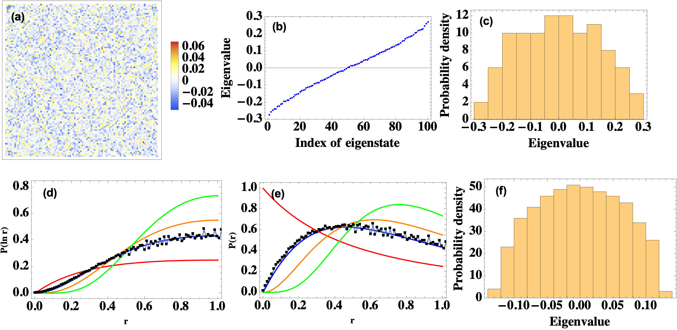
Figure 1: (a) The random Gaussian symmetry matrix up to $D=100$, $\frac{\sqrt{\lambda_{1}^{2}+\lambda_{2}^{2}}}{D}\frac{1}{\sqrt{2}}({\bf A}+{\bf A}^{T})$, with ${\bf A}$ be the $D\times D$ matrix whose entries are sampled from a standard normal distribution. The distribution of matrix elements follows $\mathcal{N}(-0.0112,0.031)$. The eigenvalue distribution is shown in (b). (c) The histogram plot satisfies the Wigner semicircle law. (d)-(e) show the level spacing statistic for GOE (the blue, red, orange, and Green lines correspond to GOE, GUE, GSE, and Poission, respectively). (f) shows the diagram corresponding to $D=500$.

Thus the effect of phase only emerges in finite chemical potential or for nonlocal Cooper susceptibility. This is diagrammatically shown in Fig.1, where a Cooper pair is scattered back to the original site $\alpha$ through the interaction with another Cooper pair which scattered back to site $\beta$. Here we obtain another gap equation

$$\frac{\Sigma_{A}^{0}}{g}=\frac{-g\Delta_{0}}{g}=-\Delta_{0},$$ (105)

where $\Delta_{0}$ plays the role of anomalous Green's function. The relations between $\Sigma_{A}^{0}$, $\Delta_{0}$, $\Pi_{b}^{0}$, $\Pi_{b}$ and $G_{f}$ are concluded in Fig.1. And in a word, if $g\neq 0$, the pair condensation happen only in the case that $\Pi_{b}\rightarrow 0$ while $\Sigma_{A}^{0}\sim|\Delta_{0}|\rightarrow\infty$.

In IR limit and free fermion limit ($J\rightarrow 0$), we have

$$|\Delta_{0}(0)|\sim\Pi_{b}(0)\sim-1.$$ (106)

In this case, when $m_{0}-\Pi_{b}(0)<0$, i.e., $m_{0}<-1$, the boson begins to condense, and the non-Fermi liquid phase only emergent in the critical point $m_{0}=-1$. This is different to the system described in Ref.[24] where the emergence of non-Fermi liquid requires a low-energy cutoff performed to the expression of $\Pi_{b}(0)$, we only need to turn the bare boson mass here. The key reason for this difference is the effect of $\Sigma_{A}^{0}$. We also found that $F(\omega)$ and $\Delta_{0}(\omega)$ have the same divergent behavior in IR limit in non-Fermi liquid phase, while they behave differently when boson condenses.

Now the free fermion Green's function reads

$$G_{f}(\omega)=\frac{2i}{\omega+{\rm sgn}[\omega]\sqrt{-4g+\omega^{2}}},$$ (107)

then through the same procedure (Eq.(82)), we have

$$\rho(\omega)=\frac{1}{i\pi\sqrt{g}}\sqrt{1+\frac{\omega^{2}}{4g}}.$$ (108)

Note that this is for the case $J=0$.

As discussed above, the term with $\Delta_{0}(\tau)\Delta_{0}^{{\dagger}}(\tau)$ in the action Eq.(87) cannot forms a correlator due to a single time-dependence. In fact, a nonzero $\langle\Delta_{0}(\tau)\Delta_{0}^{{\dagger}}(\tau^{\prime})\rangle$ requires finite value of $g_{q}\Phi_{il}\Phi_{jk}$, i.e., when the constant $g$ is embeded into the Gaussian distributed SYK coupling as the anomalous component. When this happen, the semicircle distribution of $g_{q}\Phi_{il}\Phi_{jk}$, which reads

$$\rho(\lambda)=\frac{1}{2\pi J^{2}}\sqrt{4J^{2}-\lambda^{2}},$$ (109)

will be replaced by

$$\rho(\lambda)=\frac{1}{2\pi J^{2}}\sqrt{4J^{2}-(\lambda-g)^{2}}\Theta(\lambda)+\frac{1}{2\pi J^{2}}\sqrt{4J^{2}-(\lambda+g)^{2}}\Theta(-\lambda)+\frac{1}{2\pi J}\delta(\lambda-g)+\frac{1}{2\pi J}\delta(\lambda+g).$$ (110)

Now the mean value of eigenvalues is still

$$\overline{\lambda}=|\int d\lambda\lambda\rho(\lambda)|=\frac{4J}{3\pi}.$$ (111)

So the correlation effect, if exists, will not be affected by the anomalous term.

6.3 Gaussian random variable $\Phi_{i}$ and $\Phi^{q}$: Random local field

Following the model presented in above subsection, we next discuss the case that each Cooper pair contains two fermions with random polaronic momenta in opposite directions, and in the mean time the on-site potential is random in strength. This is the ramdom local field case, which has recently being experimentally detected in Sr₂CuTe_0.5W_0.5O₆[28], and in contrast to the many-body local field case, as we studied above, its ratios of adjacent level spacings follows the Wigner-Dyson level statistic according to eigenstate thermalization hypothesis[27], while that in the many-body local field case follows the Poisson level statistic.

In this case, the $g$-related polaron Hamiltonian reads

$$H_{g}=-\sum_{pk,q}c_{p-\frac{q}{2}}^{{\dagger}}c_{k+\frac{q}{2}}^{{\dagger}}c_{p+\frac{q}{2}}c_{k-\frac{q}{2}},$$ (112)

which can still be written as

$$H_{g}= -g\frac{\Lambda_{q}}{N}\sum_{ij}^{N}\sum_{qq^{\prime}}^{\Lambda_{q}}\Phi^{q}\Phi^{q^{\prime}}c_{i}^{{\dagger}}d_{i}^{{\dagger}}d_{j}c_{j}=-gN\Delta_{0}^{{\dagger}}\Delta_{0}$$ (113)

where we can define the following pair propagators, as long as $\Phi_{i}$ is a Gaussian variable with $\overline{\Phi_{i}}=0,\overline{\Phi_{i}^{2}}=\frac{1}{N}$,

$$\Delta_{0}^{{\dagger}}= \frac{\sqrt{\Lambda_{q}}}{N}\sum_{i}\sum_{q}\Phi^{q}\Phi_{i}c_{i}^{{\dagger}}d_{i}^{{\dagger}},$$ (114)

$$\Delta_{0}= \frac{\sqrt{\Lambda_{q}}}{N}\sum_{j}\sum_{q^{\prime}}\Phi^{q^{\prime}}\Phi_{j}d_{j}c_{j},$$

So now the paring vertex ((Cooper susceptibility)^1/2) reads

$$\Sigma_{A}^{0}(\omega)= -gT\sum_{\Omega}\Sigma_{A}^{0}(\omega+\Omega)G_{f}(\omega)G_{f}(\Omega)\Delta_{0}(\omega-\Omega).$$ (115)

This is consistent with the anomalous self-energy obtained above, and then the Hamiltonian can be rewritten as

$$H_{g}= -gN\Delta_{0}^{{\dagger}}\Delta_{0}=-\frac{N}{g}\lambda_{b}=-\frac{N}{g}\Sigma_{A}^{0{\dagger}}\Sigma_{A}^{0}$$ (116)

$$= -\frac{N}{g}(-gT\sum_{\Omega}\Sigma_{A}^{0}(\omega+\Omega)G_{f}(\omega)G_{f}(\Omega)\Delta_{0{\dagger}}(\omega-\Omega^{\prime}))(-gT\sum_{\Omega^{\prime}}\Sigma_{A}^{0{\dagger}}(\omega+\Omega^{\prime})G_{f}(\Omega^{\prime})G_{f}(\omega)\Delta_{0}(\omega-\Omega^{\prime}))$$

$$= -\frac{N}{g}(T\sum_{\Omega}\Sigma_{A}^{0}(\omega+\Omega)G_{f}(\omega)G_{f}(\Omega)\Sigma_{A}^{0{\dagger}}(\omega-\Omega^{\prime}))(T\sum_{\Omega^{\prime}}\Sigma_{A}^{0{\dagger}}(\omega+\Omega^{\prime})G_{f}(\Omega^{\prime})G_{f}(\omega)\Sigma_{A}^{0}(\omega-\Omega^{\prime})),$$

which can be obtained by using the relations

$$\int d\tau e^{i\omega\tau}(\Sigma_{A}^{0}(\tau)-\Sigma_{A}^{0}(0))=T\sum_{\Omega}\Sigma_{A}^{0}(\omega+\Omega),$$ (117)

$$\int d\tau e^{-i\omega\tau}(\Sigma_{A}^{0}(0)-\Sigma_{A}^{0}(\tau))=T\sum_{\Omega}\Sigma_{A}^{0}(\omega-\Omega).$$

Then, similar to the discussion presented in Sec.4, if we summing over the $q$ superscripts before the disorder average over fermion indices $ij$,

$$\Delta_{0}=\frac{1}{N}\sum_{i}d_{i}c_{i}=\frac{1}{N}\sum_{i}(\sum_{q}\Phi^{q}d_{i}c_{i}),$$ (118)

then, when $2\Lambda_{q}^{-1}=N$, the $N\times N$ matrix $H_{g}$ can be diagonalized to has $N$ eigenstates with the corresponding eigenvalues $\pm g\frac{1}{4\Lambda_{q}^{-1}N}$. In this case, all eigenvalues are very small in large $N$ (or $\Lambda_{q}^{-1}$) limit. While if we firstly calculate the disorder average over the $q,q^{\prime}$ indices and then the $ij$ indices,

$$\Delta_{0}=\frac{1}{N}\sum_{i}d_{i}c_{i}=\frac{\sqrt{\Lambda_{q}}}{N}\sum_{i}\sum_{q}\Phi^{q}d_{i}c_{i},$$ (119)

then $H_{g}$ is still a $N\times N$ matrix, but now each of its diagonal eigenmodes has a eigenvalue of order of $\Lambda_{q}^{-1/2}$, i.e., with stiffness that extensive in $\Lambda_{q}^{-1/2}$ which suppresses the O(N) fluctuation to the conformal saddel point, and even spoils the mean-field solution (with infinite dimension) when the value of $N$ and $\Lambda_{q}^{-1/2}$ are comparable. But note that the latter case only valid in large $N,\Lambda_{q}^{-1/2}$ case.

Inspired by the truth that on-site random potential can be described by the $H_{\flat=2}$ -like model[25], once $\Phi_{i}$ and $\Phi^{q}$ are Gaussian random variables, the conformal saddle-point can be found even with constant $g$. Firstly, we write the partition function as

$$e^{-H_{g}}=\int D\psi e^{-\frac{1}{g}\psi_{1}\psi_{2}-i\psi_{1}\Phi_{i}c_{i}^{{\dagger}}d_{i}^{{\dagger}}\Phi^{q}-i\psi_{2}\Phi_{j}d_{j}c_{j}\Phi^{q^{\prime}}}.$$ (120)

Then using identity

$$\int d\Phi^{q}_{i}d(\Phi^{q}_{i})^{*}e^{-\frac{1}{\sigma^{2}}(\Phi_{i}^{q}-i\sigma^{2}\psi_{1}^{*}d_{i}c_{i})(\Phi_{i}^{q*}+i\sigma^{2}\psi_{1}c_{i}^{{\dagger}}d_{i}^{{\dagger}})}=e^{\sigma^{2}\psi^{*}_{1}\psi_{1}d_{i}c_{i}c_{i}^{{\dagger}}d_{i}^{{\dagger}}},$$ (121)

where the variance reads

$$\sigma^{2}=g\overline{(\Phi_{i}^{q})^{2}}=\overline{(\Phi_{i})^{2}}\overline{(\Phi^{q})^{2}}=g\frac{2\Lambda_{q}}{N}.$$ (122)

Then the action reads

$$S= \int d\tau(\sum{iq}c_{i}^{{\dagger}}[\partial_{\tau}+\Sigma_{A}^{0}]d_{i}^{{\dagger}}+\sum{jq^{\prime}}d_{j}[\partial_{\tau}+\Sigma_{A}^{0{\dagger}}]c_{j}+\frac{1}{g}\psi_{1}\psi_{2})$$ (123)

$$-g\int d\tau d\tau^{\prime}2N(\psi_{1}^{*}(\tau)\psi_{1}(\tau^{\prime})+\psi_{2}^{*}(\tau)\psi_{2}(\tau^{\prime}))\Delta_{0}(\tau)\Delta_{0}^{{\dagger}}(\tau^{\prime})$$

$$-\int d\tau\frac{N}{\sqrt{\Lambda_{q}}}\Sigma_{A}^{0{\dagger}}(\tau)\Delta_{0}(\tau)-\int d\tau\frac{N}{\sqrt{\Lambda_{q}}}\Sigma_{A}^{0}(\tau)\Delta^{{\dagger}}_{0}(\tau).$$

Then we obtain the unstable conformal saddle-point (mean-field solution form)

$$\Delta_{0}=\frac{1}{\sqrt{\Lambda_{q}}}\frac{1}{i\omega-\Sigma_{A}^{0}},$$ (124)

$$\Sigma_{A}^{0}=-2\sqrt{\Lambda_{q}}(\psi_{1}^{*}\psi_{1}+\psi^{*}_{2}\psi_{2})\Delta_{0}^{{\dagger}},$$

where the factor $\Lambda_{q}^{1/2}$ induces fluctuation to the saddle-point.

By keeping the $g$-related term invariant under the scaling $\tau\rightarrow B\tau$, we have $\psi\rightarrow B^{-1/2}\psi$, $c\rightarrow B^{-1/4}c$. That is to say, as long as $\Phi_{i}$ and $\Phi^{q}$ are Gaussian variables, it is possible to make the random-$g$-dependent term and $J$-dependent term (see Appendix.B) be scaling invariant in the same time, and thus the on-site interaction with random strength will not be a perturbation to the $H_{\flat=4}$ model, i.e., it does not have a competition with the $J$-dependent SYK term (see Appendix.B). While in the case that $\psi$ is time-independent, i.e., its propagator are completely screened, the random-$g$-dependent term behaves like a $H_{\flat=2}$ model and thus support a disordered fermi-liquid phase. If $\psi\rightarrow B^{x}\psi$ ($x>0$), the fermionic field has an anomalous scaling $c\rightarrow B^{-\frac{1+x}{2}}c$ with $-\frac{1+x}{2}<-1/2$. For $\psi$ field, a negative scaling dimension is possible for each boson mode $\psi$ in the correlator form as verified in random-bond Ising model[29]. And here the random-bond is also being mentioned in Ref.[28], where the induced bond disorder together with random local field effect contribute to the SYK physics, including the stable quantum spin liquid. But note that the precondition for all these is that the $\Phi_{i}$ and $\Phi_{j}$ need to be Gaussian variables, to validate the replica procedure.

If we define $\Phi_{ij}$ (insteads of $\Phi_{i}$) as a Gaussian variable, the Hamiltonian becomes

$$H_{g}= -\int d\tau d\tau^{\prime}4gG_{c}G_{d}.$$ (125)

where we define the normal propagators as

$$G_{c}(\tau,\tau^{\prime})=\frac{\sqrt{\Lambda_{q}}}{2\sqrt{N}}\sum_{ij}\sum_{qq^{\prime}}\sqrt{\Phi^{q}\Phi^{q^{\prime}}}c_{i}^{{\dagger}}(\tau^{\prime})c_{j}(\tau),$$ (126)

$$G_{d}(\tau,\tau^{\prime})=\frac{\sqrt{\Lambda_{q}}}{2\sqrt{N}}\sum_{ij}\sum_{qq^{\prime}}\sqrt{\Phi^{q}\Phi^{q^{\prime}}}d_{i}^{{\dagger}}(\tau^{\prime})d_{j}(\tau).$$

In this case $H_{g}$ becomes a SYK${}_{q=2}\times$SYK${}_{q=2}\times$SYK${}_{\flat^{\prime}=1}\times$SYK${}_{\flat^{\prime}=1}$ model.

Note that since we define $\Phi^{q}$ ($\Phi^{q^{\prime}}$) as a Gaussian variable, the $\Phi^{q}\Phi^{q^{\prime}}$ is a Chi-square variable, and there exist the following disorder averages over $q$ (which is completely independent with $q^{\prime}$) and $q^{\prime}$

$$\overline{\Phi^{q}}=0,$$ (127)

$$\overline{\Phi^{q}\Phi^{-q}}=\overline{(\Phi^{q})^{2}}=\overline{(\Phi^{-q})^{2}}=2\Lambda_{q},$$

$$\overline{\Phi^{q}\Phi^{q^{\prime}}}=\overline{\Phi^{q}}\overline{\Phi^{q^{\prime}}}=0,$$

$$\overline{(\Phi^{q}\Phi^{q^{\prime}})^{2}}=\overline{(\Phi^{q})^{2}}\overline{(\Phi^{q^{\prime}})^{2}}=4\Lambda_{q}^{2}.$$

There is an important difference between disorder average over the fermion indices and the polaronic $q$ indices, when the fermion scale is $\flat^{\prime}=1$. This is because that, different to the fermion (site) indices, each polaronic momentum $q$ can takes two possible directions, which can not all be accounted during the summation, but should all be accounted during the disorder average. To be clear, we write the summation and disorder average over the fermion indices and polaronic momenta, respectively, in the following. For fermion indices:

$$\overline{\Phi_{i}}=0,\sum_{i}^{N}\Phi_{i}=\overline{\Phi_{i}}N=0,\overline{\Phi_{i}^{2}}=\frac{2\mathcal{O}_{i}^{{\dagger}}\mathcal{O}_{i}}{2N}=\frac{1}{N}.$$ (128)

For polaronic momentum indices:

$$\overline{\Phi^{q}}=0,\sum_{q}^{\Lambda_{q}}\Phi^{q}=\overline{\Phi^{q}}\Lambda_{q}^{-1}=0,\overline{(\Phi^{q})^{2}}=2\frac{2\mathcal{O}_{q}^{{\dagger}}\mathcal{O}_{q}}{2\Lambda_{q}^{-1}}=2\Lambda_{q}.$$ (129)

7 Symmetry classes

Note that, as we assume that both the nonlocal interaction $g_{q}$ and the local one $g$ are charge-conserving interactions, there is always a global U(1) charge symmetry which is the only unitary symmetry here. So the related SYK Hamiltonians can be block diagonalized in the sector of eigenvalues of glocal U(1) charge $\mathcal{Q}$ as obtained in Appendix.C, which is $\mathcal{Q}=\sum^{N}_{i}(c^{{\dagger}}_{i}c_{i}-1/2)=-\theta/\pi$, and with eigenvalues $\lambda^{\pm}_{Q}=\pm\sum^{N}_{i}(n_{i}-1/2)$. For nonzero $\lambda_{Q}$, there is an antiunitary symmetry $\mathcal{S}\mathcal{Q}\mathcal{S}^{-1}=-\mathcal{Q}$, which makes the system has a twofold spectral degeneracy by the mapping the $\lambda^{+}_{Q}$ sector to $\lambda^{-}_{Q}$ sector. This antiunitary symmetry includes the chiral symmetry, time-reversal symmetry, and even the particle-hole symmetry, which is possible at finite chemical potential $\mu\neq 0$ before the SYK term is being fully antisymmetrized. Note that for zero chemical potential, $\lambda_{Q}=0$, and then the Wigner-Dyson matrix ensemble can only applied for even $N$[27]. Besides, we have proved that the Chi-square variable behaves like a $H_{\flat=4}$ in some ways, where we perform the level statistic (as well as the disorder average) separately for the Gaussian variables, and the GUE ensemble can be applied as long as $\Lambda_{q}^{-1}\gg N$, which provides a series of continuously distributed energy levels. While in the opposite limit $\Lambda_{q}^{-1}\ll N$, the Chi-square variable distribution is absence and there is a large degeneracy of levels at zero energy when the Gaussian distributed wave functions $\Phi_{il}$ and $\Phi_{jk}$ are mutually orthogonal, and lead to Poissonian level statistic, similar to what happen when the level statistic is collected for different symmetry sectors[27].

First we consider the chiral antiunitary symmetry class (AIII), where the time reversal symmetry is broken (while the chiral orthogonal (BDI) and chiral symplectic (CII) preserve the time reversal symmetry). The $H_{\flat=4}$ term does not has an exact four-fold periodicity in $N$ unless it is being fully antisymmetrized. While for the SYK${}_{q=2}\times$$H_{\flat=2}$ term, the level statistics should be collected seperately in each sector. Next, we firstly discuss the GUE level statistic, which does not depends on the periodicity of quantum number, like the $N$, $\Lambda_{q}^{-1}$, or $\lambda_{Q}$. For the complex Hermitian matrix $H_{\lambda_{Q}}$, we have $\mathcal{S}H_{\lambda_{Q}}\mathcal{S}^{-1}=H_{Q}=H_{-Q}^{*}$, where the antiunitary operator reads $\mathcal{S}=\mathcal{U}\mathcal{K}$ with $\mathcal{U}=\begin{pmatrix}0&1\\ \mathcal{S}^{2}&0\end{pmatrix}$ the unitary operator and $\mathcal{K}$ the complex conjugation operator. In this case, we have $\mathcal{S}^{2}=\mathcal{U}\mathcal{U}^{*}=(-1)^{N}$. The GOE and GSE (Gaussian symplectic emsemble) level statistic only appear at $\lambda_{Q}=0$, where $\mathcal{S}^{2}=1$ with $\mathcal{U}=\begin{pmatrix}0&1\\ 1&0\end{pmatrix}$ for GOE and $\mathcal{S}^{2}=-1$ with $\mathcal{U}=\begin{pmatrix}0&1\\ -1&0\end{pmatrix}$ for GSE.

To discuss the case of GOE and GSE at nonzero $\lambda_{Q}$, we focus on the chiral symplectic (CII) symmetry class, and introduce the following antiunitary symmetries: time-reversal symmetry ($\mathcal{T}c\mathcal{T}^{-1}=c^{{\dagger}},\mathcal{T}c^{{\dagger}}\mathcal{T}^{-1}=-c,\mathcal{T}H\mathcal{T}^{-1}=H$) and particle-hole symmetry ($\mathcal{C}c\mathcal{C}^{-1}=c^{{\dagger}},\mathcal{C}c^{{\dagger}}\mathcal{C}^{-1}=c,\mathcal{C}\mathcal{Q}\mathcal{C}^{-1}=-\mathcal{Q}^{*}$, $\mathcal{C}H\mathcal{C}^{-1}=H^{*}$), and the $\mathcal{S}$ reads $\mathcal{S}=\mathcal{T}\mathcal{C}\mathcal{K}$ where we omit the U(1) symmetry exponential part. Note that here the particle-hole symmetry operation looks exactly like the complex conjugation operation, but indeed the particle-hole symmetry also related to the spin index of the fermion operator, which can be seen when the SU(2) symmetry is being considered. In CII symmetry class, we have $\mathcal{T}^{2}=(-1)^{N}$ and $\mathcal{C}^{2}=(-1)^{\lambda_{Q}}$ and $\mathcal{S}^{2}=\mathcal{T}^{2}\mathcal{C}^{2}=(-1)^{N+\lambda_{Q}}$[33]. And we can write

$$\mathcal{S}H_{\lambda_{Q}}\mathcal{S}^{-1}= \mathcal{T}\mathcal{C}\mathcal{K}H_{\lambda_{Q}}\mathcal{K}^{-1}\mathcal{C}^{-1}\mathcal{T}^{-1}$$ (130)

$$= \mathcal{T}\mathcal{C}H^{*}_{\lambda_{Q}}\mathcal{C}^{-1}\mathcal{T}^{-1}$$

$$= \mathcal{T}H_{\lambda_{Q}}\mathcal{T}^{-1}$$

$$= H_{\lambda_{Q}}=H_{-\lambda_{Q}},$$

where $\mathcal{S}^{2}=1$ for GOE with even $N+\lambda_{Q}$ and $\mathcal{S}^{2}=-1$ for GSE with odd $N+\lambda_{Q}$. This discuss for the CII class can also be performed by using the charge conjugation operator $\mathcal{C}^{{}^{\prime}}=\mathcal{K}\mathcal{C}$ ($\mathcal{C}^{\prime}\mathcal{Q}\mathcal{C}^{{}^{\prime}{\dagger}}=-\mathcal{Q}$, $\mathcal{C}^{\prime}H\mathcal{C}^{{}^{\prime}{\dagger}}=H$), and then $\mathcal{S}=\mathcal{T}\mathcal{C}^{{}^{\prime}{\dagger}}$. In this case, the time reversal symmetry can still be obtained by

$$\mathcal{T}H_{\lambda_{Q}}\mathcal{T}^{-1}= \mathcal{S}\mathcal{C}^{\prime}H_{\lambda_{Q}}\mathcal{C}^{{}^{\prime}{\dagger}}\mathcal{S}^{-1}$$ (131)

$$= \mathcal{S}H_{\lambda_{Q}}\mathcal{S}^{-1}$$

$$= H_{\lambda_{Q}}=H_{-\lambda_{Q}}.$$

In conclusion, in BDI class, the level statistic must follows GOE as the entries of block diagonalized random Hamiltonian matrix are real. While in AIII, it follows GUE since the entries are always complex as long as $\lambda_{Q}\neq 0$. In CII class, different to the single fermion case[34, 33], the many-body time reversal symmetry does not always satisfy $\mathcal{T}^{2}=1$, so it is possible for the entries to be real (GOE) or real quaternion (GSE).

8 Conclusion

In terms of the polaronic momentum $q$, which is also the relative momentum during scattering between impurity and majority particles (or holes). The polaron forms at the pole of scattering amplitude where $q=ia^{-1}$, where $a$ is the scattering length, and the quantity $qa$ becomes an important characterisic scale in predicting the many-body behaviors. Note that we works on the condition that close to the half-filling with cutoff $\Lambda_{q}^{-1}\rightarrow\infty$ to satisfy the requirement of SYK physics. In such non-Fermi liquid phase, since the $q$ is small, and the coupling is strong, the polaron is not well-defined unlike in the Fermi liquid phase. In the opposite limit with $\Lambda_{q}^{-1}\ll N^{2}$, as we also discuss in this paper, the system exhibits (disordered) Fermi liquid features, e.g., the sharp peaks in spectral function. While in the Fermi liquid phase with well-defined Fermi surface, the above characterisic scale should be replaced by $k_{F}a$ where $k_{F}$ is the Fermi wave vector.

In conclusion, the polaron system, although formed by the four-fermion interacting term, can never be a $H_{\flat=4}$ model, but after summation over $q$-superscript (i.e., the mean value times $\Lambda_{q}^{-1}$), we can analyse the matrix in GUE by treating $g_{q}\Phi_{il\sigma}\Phi_{jk\sigma^{\prime}}$ as a $N^{2}\times N^{2}$ matrix. In this case (as long as $\Lambda_{q}\neq 0$), the variables $\Phi_{il}$ and $\Phi_{jk}$ are Gaussian, while $g_{q}\Phi_{il\sigma}\Phi_{jk\sigma^{\prime}}$ is a Chi-square variable. And in the mean time, since the $q$ component are summarized, the wave functions $\Phi_{il}$ and $\Phi_{jk}$ become completely independent. This is what we called SYK${}_{q=2}\times$SYK${}_{q=2}\times$SYK${}_{\flat^{\prime}=1}$ model, which can well describes the SYK dynamics of polaron system. Here the $\flat^{\prime}=1$ is to combine the disorder average over $\Phi^{q}$ and $\Phi^{-q}$ components into the disorder average over fermion indices. While in the long-wavelength limit ($\Lambda_{q}=0$), $\Phi_{il}$ and $\Phi_{jk}$ are no more Gaussian, but the Hamiltonian can be reconstructed to contains the Gaussian variable $\Phi_{ik}$, where $\overline{\Phi_{ik}^{2}}=\overline{\Phi_{jl}^{2}}=\frac{J}{2N}$. Also, in this case, the SYK Hamiltonian (polaron no more exists now) is positive-define, which means the eigenstates corresponding to zero eigenvalue are the ground states, and all eigenvalues of matrix $g_{q}\Phi_{il\sigma}\Phi_{jk\sigma^{\prime}}$ are positive. Lastly, we discuss the case of pair condensation, which happen at critical temperature, and leads to zero dressed (or undressed) boson self-energy. We deduce the free energy density and the divergent behaviors of anomalous propagator in this case.

During the above basis transformation between the original polaron momentum basis and the SYK fermion indices basis, in the $\Lambda_{q}^{-1}\rightarrow\infty$ limit, only the statistical relations between $\phi_{i}$ and $\phi_{l}$ or $\phi_{j}$ and $\phi_{k}$ depends on the value of $\Lambda_{q}^{-1}$, but this dependence on $\Lambda_{q}^{-1}$ is also being replaced by number $N$ after the transformation. While the disorder average over $q$ is carried out seperately with that of $N$, which is allowed only under the condition $\Lambda_{q}^{-1}\gg N^{2}$, and in this case, the SYK physics cannot be realized if we do the summation over $q$ first which requires $\Lambda_{q}^{-1}<N^{2}/2$ to realize SYK physics.

9 Appendix.A: Application of Hubbard-Stratonovich transformation and replica technique for coupled product

Using Baker–Campbell–Hausdorff formula, we can write a density matrix inclduing a coupled product $e^{x}e^{y}$ as

$${\rm ln}(e^{x}e^{y})= \sum_{i_{1}\in Z^{*},j_{1}=0,1}\frac{[x^{(i_{1})},y^{(j_{1})}]}{(i_{1}+j_{1})i_{1}!j_{1}!}+\sum_{i_{1}\in Z^{*},j_{2}=0,1}\frac{[x^{(i_{1})},[y^{(j_{1})},[x^{(i_{2})},y^{(j_{2})}]]]}{(i_{1}+j_{1}+i_{2}+j_{2})i_{1}!j_{1}!i_{2}!j_{2}!}$$ (132)

$$=x+y+\sum_{i_{1}=1}^{\infty}\frac{[x^{(i_{1})},y]}{(i_{1}+1)i_{1}!}$$

$$+\sum_{i_{1}\geq 1}\frac{[x^{(i_{1})},y]}{(i_{1}+1)i_{1}!}+\sum_{i_{1}\geq 0,j_{1}\geq 1}\frac{[x^{(i_{1})},[y^{(j_{1})},x]]}{(i_{1}+j_{1}+1)i_{1}!j_{1}!}+\sum_{i_{1}\geq 0,j_{1}\geq 1,i_{2}\geq 1}\frac{[x^{(i_{1})},[y^{(j_{1})},[x^{(i_{2})},y]]}{(i_{1}+j_{1}+i_{2}+1)i_{1}!j_{1}!i_{2}!}$$

where $[x^{(2)},y]=[x,[x,y]]$ denotes the iterated Lie bracket. We consider only to the first order where

$${\rm ln}(e^{x}e^{y})=x+y+\frac{[x,y]}{2}.$$ (133)

Then we have

$$e^{x}e^{y}=e^{x+y+\frac{[x,y]}{2}},$$ (134)

$$e^{x}e^{y}e^{-x}=e^{y+[x,y]},$$

$$e^{-y}e^{x}e^{y}=e^{x+[x,y]},$$

which are consistent with inserting an operator identity through the Baker-Hausdorff lemma,

$$e^{x}e^{y}e^{-x}=e^{y}+[x,e^{y}]=e^{y}(1+\frac{[x,e^{y}]}{e^{y}})=e^{y}(1+[x,y])=e^{y}e^{[x,y]}=e^{y+[x,y]},$$ (135)

$$e^{-y}e^{x}e^{y}=e^{x}+[-y,e^{x}]=e^{x}(1+\frac{[-y,e^{x}]}{e^{x}})=e^{x}(1+[-y,x])=e^{x}e^{[-y,x]}=e^{x+[x,y]}.$$

Next we consider the Hamiltonian $h=e^{a}e^{b}$ where $[a,b]\neq 0$, the corresponding density matrix is $e^{-h}$. To perform the Hubbard-Stratonovich transformation, we introduce the identity

$$\int\mathcal{D}[\psi]e^{-\psi_{1}\psi_{2}}=1.$$ (136)

In terms of the corresponding linear response of effective Hamiltonian, we have another set of variable $\hat{\psi}_{1},\hat{\psi}_{2}$ that share the similar identity with $\psi_{1},\psi_{2}$:

$$\hat{\psi}_{1}=\psi_{1}+\sum_{i}e^{a}_{i}x_{i},$$ (137)

$$\hat{\psi}_{2}=\psi_{2}+\sum_{j}e^{b}_{j}x_{j},$$

where

$$\int\mathcal{D}[\hat{\psi}]e^{-\hat{\psi}_{1}\hat{\psi}_{2}}=1,$$ (138)

implies the variable set $\psi_{1},\psi_{2}$ can be viewed as a saddle-point case of $\hat{\psi}_{1},\hat{\psi}_{2}$ which is specified by certain saddle-point coordinator-dependence (linearly independent of others), in terms of the fluctuational expansion around saddle-point. The latter terms describe the fluctuations, a set of coupled coefficients $x_{i},x_{j}$ ($[x_{i},x_{j}]\neq 0$) successfully decoupes the two sums including the taylor-expanded exponential terms $e^{a}$ and $e^{b}$, and in the mean time without change their product,

$$\sum_{i}e^{a}_{i}x_{i}\sum_{j}e^{b}_{j}x_{j}=e^{a}e^{b}=e^{a+b+\frac{[a,b]}{2}}.$$ (139)

From this, we can write the effective susceptibility as

$$\frac{\delta x_{j}}{\delta\phi_{i}}=\langle x_{i}x_{j}\rangle=\frac{\sum_{i}e^{a}_{i}x_{i}\sum_{j}e^{b}_{j}x_{j}}{\sum_{i}e^{a}_{i}\sum_{j}e^{b}_{j}}=e^{\frac{[a,b]}{2}},$$ (140)

where the corresponding symmetry property can be observed in terms of the zero functional derivatives of $x_{i}$ with respect to the bosonic source field $\phi_{i}$. The corresponding linear response is

$$e^{-\beta H}\rightarrow e^{-\beta H}\mathcal{T}e^{\int d\tau x_{i}(\tau)\phi_{i^{\prime}}(\tau)},$$ (141)

where through bosonization we have $x_{i}=\partial_{i}\phi_{i}$,

$$\int d\tau(\partial_{i}\phi_{i}(\tau))\phi_{i^{\prime}}(\tau)=i\delta_{ii^{\prime}}+\int d\tau\phi_{i^{\prime}}(\tau)(\partial_{i}\phi_{i}(\tau)),$$ (142)

with the delta-function in vacuum expectation-type definition: $i\delta_{ii^{\prime}}=\frac{1}{i-i^{\prime}-{\bf i}0^{+}}+\frac{1}{i^{\prime}-i-i0^{+}}$. In terms of density matrix and the correlation function in a basis of initial state $\psi$,

$$\frac{\delta\langle x_{j}\rangle_{\psi}}{\delta\phi_{i}}=\langle x_{i}x_{j}\rangle_{\psi}={\rm Tr}[x_{i}x_{i^{\prime}}e^{\tau_{j}H_{j}}e^{-\tau_{j}H_{j}}]=\frac{{\rm Tr}[x_{i}e^{(\tau_{j}-\Delta\tau_{i})H_{j}}x_{i^{\prime}}e^{-\tau_{j}H_{j}}]}{{\rm Tr}[e^{-\Delta\tau_{i}}]}$$ (143)

where we consider the a Hermitian case whose expectation is evaluated through a microcanonical ensemble at thermal equilibrium $e^{\tau_{j}H_{j}}e^{-\tau_{j}H_{j}}$ which bring the corresponding microcanonical ensemble's character as carriered by $\tau_{j}$.

The corresponding conservation can be projected to the exponential integral over the disordered Gaussian-distributed variables

$$\int\mathcal{D}[\hat{\psi}]e^{-(\psi_{1}\psi_{2}-\hat{\psi}_{1}\hat{\psi}_{2})}=1.$$ (144)

$$e^{-e^{a}e^{b}}=\int\mathcal{D}[\hat{\psi}]e^{-\hat{\psi}_{1}\hat{\psi}_{2}}e^{-\psi_{1}(\sum_{j}e^{b}_{j}x_{j})}e^{-\psi_{2}(\sum_{i}e^{a}_{i}x_{i})}.$$ (145)

Next we further inserting another set of identity in terms of the Gaussian distributed variables $(\sqrt{\hat{\psi}_{1}\hat{\psi}_{2}}+\overline{\psi}_{1})$ and $(\sqrt{\hat{\psi}_{1}\hat{\psi}_{2}}+\overline{\psi}_{2})$,

$$2(\sqrt{\hat{\psi}_{1}\hat{\psi}_{2}}+\overline{\psi}_{1})\overline{\psi}_{1}+2(\sqrt{\hat{\psi}_{1}\hat{\psi}_{2}}+\overline{\psi}_{1})\overline{\psi}_{1}=\psi_{1}(\sum_{j}e^{b}_{j}x_{j})+\psi_{2}(\sum_{i}e^{a}_{i}x_{i}),$$ (146)

which indeed corresponds to the invariance provided by Eq.(144),

$$\overline{(\sqrt{\hat{\psi}_{1}\hat{\psi}_{2}}+\overline{\psi}_{1})^{2}}=\overline{(\sqrt{\hat{\psi}_{1}\hat{\psi}_{2}}+\overline{\psi}_{2})^{2}}=\overline{(\hat{\psi}_{1}\hat{\psi}_{2}-\psi_{1}\psi_{2})}.$$ (147)

Then we have

$$e^{-e^{a}e^{b}}=\int\mathcal{D}[\hat{\psi}]\int\mathcal{D}[\overline{\psi}]e^{-\hat{\psi}_{1}\hat{\psi}_{2}}e^{(\overline{\psi_{1}})^{2}}e^{(\overline{\psi_{2}})^{2}},$$ (148)

where using Eq.(147) we can obtain

$$\overline{-\psi_{1}\psi_{2}}=\overline{-(\overline{\psi}_{1})^{2}+\psi_{1}(\sum_{j}e^{b}_{j}x_{j})}=\overline{-(\overline{\psi}_{2})^{2}+\psi_{2}(\sum_{i}e^{a}_{i}x_{i})}.$$ (149)

In this way, the density matrix $h$ has been decouped, in terms of path integral representation, to actions including the fermion Green function ($G$) and boson Green function ($D$):

$$G_{1}(\tau-\tau^{\prime})=\overline{\psi}_{1}(\tau)\overline{\psi}_{1}(\tau^{\prime}),$$ (150)

$$G_{2}(\tau-\tau^{\prime})=\overline{\psi}_{2}(\tau)\overline{\psi}_{2}(\tau^{\prime}),$$

$$\hat{D}(\tau-\tau^{\prime})=\hat{\psi}_{1}(\tau)\hat{\psi}_{2}(\tau^{\prime}).$$

Inserting the identity where the bosonic self-energy $\hat{\Sigma}$ plays the role of Lagrange multipliers

$$\int\mathcal{D}[\hat{\Sigma}]\mathcal{D}[\hat{D}]e^{-\int d\tau\int d\tau^{\prime}\hat{\Sigma}(\tau-\tau^{\prime})(\hat{D}(\tau-\tau^{\prime})-\hat{\psi}_{1}(\tau)\hat{\psi}_{2}(\tau^{\prime}))}=1,$$ (151)

whose static solutions are available through saddle-point approximation

$$e^{-e^{a}e^{b}} =\int\mathcal{D}[\hat{\psi}]\int\mathcal{D}[\overline{\psi}]e^{-\int d\tau\int d\tau^{\prime}\hat{\psi}_{1}(\tau)(\partial_{\tau}\delta_{\tau,\tau^{\prime}}-\hat{\Sigma})\hat{\psi}_{2}(\tau^{\prime})}e^{-\hat{\Sigma}\hat{D}}e^{\overline{G}_{1}}e^{\overline{G}_{2}}$$ (152)

10 Appendix.B: Numerical simulations for GOE

In random matrix theory (RMT), the distributions are studied in terms of correlation functions of products. The case of half-integer ($\beta=1$) powers of characteristic polynomials of random matrices corresponds to the Gaussian orthogonal ensemble (GOE). Tradictionally, a $N\times N$ GOE matrix $\bf{O}$ has the following property: the distribution of ${\bf O}$ is the same with ${\bf U}^{T}{\bf O}{\bf U}$. where ${\bf U}$ is the non-random $N\times N$ orthogonal matrix such that ${\bf U}^{T}{\bf U}={\bf I}$. As an example, we consider two nondegenerated eigenstates for ${\bf O}$, with the corresponding individual eigenvalues $\lambda_{1},\lambda_{2}$,

$${\bf O}=\begin{pmatrix}{\rm cos}\theta&-{\rm sin}\theta\\ {\rm sin}\theta&{\rm cos}\theta\end{pmatrix}\begin{pmatrix}\lambda_{1}&0\\ 0&\lambda_{2}\end{pmatrix}\begin{pmatrix}{\rm cos}\theta&{\rm sin}\theta\\ -{\rm sin}\theta&{\rm cos}\theta\end{pmatrix}=\begin{pmatrix}\lambda_{1}\cos^{2}\theta+\lambda_{2}\sin^{2}\theta&(\lambda_{1}-\lambda_{2})\cos\theta\sin\theta\\ (\lambda_{1}-\lambda_{2})\cos\theta\sin\theta&\lambda_{1}\sin^{2}\theta+\lambda_{2}\cos^{2}\theta\end{pmatrix}.$$ (153)

The above expression equivalents to the non-Hermitian form $\langle m|{\bf O}|m^{\prime}\rangle$ in terms of a set of eigenkets of a real symmetric random matrix $\{|m\rangle\}=|\alpha\rangle,|\beta\rangle,|\gamma\rangle,|\eta\rangle$, whose corresponding Hilbert space dimension is $D$,

$${\bf O}=\begin{pmatrix}\sum_{i}\lambda_{i}\psi^{2}_{\alpha,i}&\sum_{i}\lambda_{i}\psi_{\alpha,i}\psi_{\beta,i}\\ \sum_{i}\lambda_{i}\psi_{\beta,i}\psi_{\alpha,i}&\sum_{i}\lambda_{i}\psi^{2}_{\beta,i}\end{pmatrix}$$ (154)

where $\psi_{\alpha,1}=\cos\theta$, $\psi_{\beta,1}=\sin\theta$, $\psi_{\alpha,2}=-\sin\theta$, $\psi_{\beta,2}=\cos\theta$. Obviosuly the above case corresponds to the integrable case, and the sum of diagonal elements is the sum of eigenvalues ($\lambda_{1}+\lambda_{2}$); While for the nonintegrable one, using Berry’s conjecture, the sum of diagonal elements including an additional term, which is the Gaussian random variables multipled by a classical analog of the (Hilbert space dimension-dependent) average shape of eigenfunctions. Such proximity for elements $\langle m|{\bf O}|m^{\prime}\rangle$ to the Berry’s conjecture expression requires $D\geq 4$ As an example, we consider $D=4$, then there is one possible eigenvector set

$$\psi_{\alpha,1}=\frac{1}{\sqrt{8}}(X_{1}\cos\theta,Y_{1}\sin\theta,\cos\theta,\cos\theta),\psi_{\beta,1}=\frac{1}{\sqrt{8}}(-\sin\theta,-\cos\theta,-\sin\theta,-\sin\theta),$$ (155)

$$\psi_{\eta,1}=\frac{1}{\sqrt{8}}(\cos\theta,\cos\theta,X_{2}\cos\theta,Y_{2}\sin\theta),\psi_{\gamma,1}=\frac{1}{\sqrt{8}}(-\sin\theta,-\sin\theta,-\sin\theta,-\cos\theta),$$

$$\psi_{\alpha,2}=\frac{1}{\sqrt{8}}(\sin\theta,-\cos\theta,\sin\theta,\sin\theta),\psi_{\beta,2}=\frac{1}{\sqrt{8}}(X_{1}\cos\theta,-Y_{1}\sin\theta,\cos\theta,\cos\theta),$$

$$\psi_{\eta,2}=\frac{1}{\sqrt{8}}(\sin\theta,\sin\theta,\sin\theta,-\cos\theta),\psi_{\gamma,2}=\frac{1}{\sqrt{8}}(\cos\theta,\cos\theta,X_{2}\cos\theta,-Y_{2}\sin\theta).$$

10.1 Second and fourth moment

Using the properties of GOE,

$$\overline{\langle m|{\bf O}|m\rangle^{2}}=\overline{(\sum_{i}\lambda_{i}|\psi_{m,i}|^{2})^{2}}=\lambda_{1}^{2}\overline{|\psi_{m,1}|^{4}}+\lambda_{2}^{2}\overline{|\psi_{m,2}|^{4}}+2\lambda_{1}\lambda_{2}\overline{|\psi_{m,1}|^{2}|\psi_{m,2}|^{2}},$$ (156)

$$\overline{\langle m|{\bf O}|m\rangle}^{2}=\overline{(\sum_{i}\lambda_{i}|\psi_{m,i}|^{2})}^{2}=\lambda_{1}^{2}\overline{|\psi_{m,1}|^{2}}^{2}+\lambda_{2}^{2}\overline{|\psi_{m,2}|^{2}}^{2}+2\lambda_{1}\lambda_{2}\overline{|\psi_{m,1}|^{2}}\ \overline{|\psi_{m,2}|^{2}},$$

$$\overline{\langle m|{\bf O}|m^{\prime}\rangle^{2}}=\overline{(\sum_{i}\lambda_{i}\psi_{m,i}\psi_{m^{\prime},i}^{*})^{2}}=\lambda_{1}^{2}\overline{|\psi_{m,1}|^{2}|\psi_{m^{\prime},1}|^{2}}+\lambda_{2}^{2}\overline{|\psi_{m,2}|^{2}|\psi_{m^{\prime},2}|^{2}}=(\lambda_{1}^{2}+\lambda_{2}^{2})\overline{|\psi_{m,2}|^{2}|\psi_{m^{\prime},2}|^{2}},$$

where the second and fourth moments in GOE satisfy

$$\overline{|\psi_{m,1}|^{2}|\psi_{m,2}|^{2}}=\overline{|\psi_{m,1}|^{2}}\ \overline{|\psi_{m,2}|^{2}}=\frac{1}{D^{2}},$$ (157)

$$\lambda_{1}^{2}\overline{|\psi_{m,1}|^{4}}+\lambda_{2}^{2}\overline{|\psi_{m,2}|^{4}}=(\lambda_{1}^{2}+\lambda_{2}^{2})\overline{|\psi_{m,1}|^{4}}=\frac{2}{D^{2}}(\lambda_{1}^{2}+\lambda_{2}^{2}).$$

Base on these relations, one set of possible solution is

$$X_{1}=-2.86-1.28i,X_{2}=0.86+1.28i,Y_{1}=-0.997+3.67i,Y_{2}=3.31-0.332i.$$ (158)

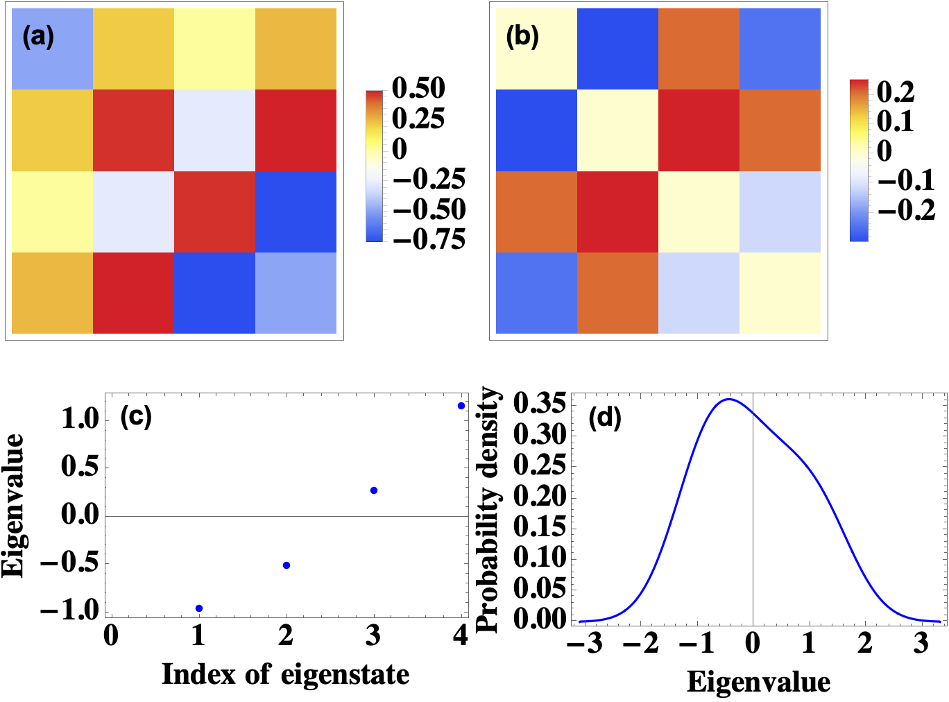
Figure 2: Approximated GOE matrix where the parameters of product variables are determined in terms of the second and fourth moment of GOE. For low $D$, we use the smoothed histogram diagram to reflect the probability density distribution.

As shown in Fig.2, the resulting matrix is not real GOE matrix as there are complex diagonal elements,

$$\left(\begin{array}[]{cccc}-0.5+5.384581669\times 10^{-15}i&0.232099\,-0.299422i&0.0201186\,+0.209108i&0.269765\,-0.250628i\\ 0.232099\,-0.299422i&0.5\,-5.38458\times 10^{-15}i&-0.269765+0.250628i&0.520119\,+0.209108i\\ 0.0201186\,+0.209108i&-0.269765+0.250628i&0.5\,-3.33066\times 10^{-15}i&-0.772336-0.118794i\\ 0.269765\,-0.250628i&0.520119\,+0.209108i&-0.772336-0.118794i&-0.5+3.33066\times 10^{-15}i\\ \end{array}\right)$$ (159)

with the complex eigenvalues $1.17-0.13i,-0.94-0.18i,-0.5+0.12i,0.27+0.18i$. However, the real part of joint distribution for the matrix entries and the eigenvalues relative to Lebesgue measure follows exactly the characters of GOE,

$$\prod_{m}^{D}\frac{1}{\sqrt{4\pi}}e^{-\frac{1}{4}O_{mm}^{2}}\prod_{1\leq m<m^{\prime}\leq D}^{D}\frac{1}{\sqrt{2\pi}}e^{-\frac{1}{2}O_{mm^{\prime}}^{2}}=(2\pi)^{-\frac{D(D+1)}{4}}\frac{1}{(\sqrt{2})^{D}}e^{-\frac{1}{4}{\rm Tr}[{\bf O}{\bf O}^{T}]},$$ (160)

$$\prod_{i}^{D}e^{\frac{-\lambda^{2}_{i}}{2}}=\prod_{m}^{D}e^{-\frac{1}{2}O_{mm}^{2}}\prod_{1\leq m<m^{\prime}\leq D}e^{-O_{mm^{\prime}}^{2}}=e^{-{\rm Tr}{\bf O}{\bf O}^{T}/2},$$

where for above example, we have (numerically)

$$\prod_{m}^{D}\frac{1}{\sqrt{4\pi}}e^{-\frac{1}{4}O_{mm}^{2}}\prod_{1\leq m<m^{\prime}\leq D}^{D}\frac{1}{\sqrt{2\pi}}e^{-\frac{1}{2}O_{mm^{\prime}}^{2}}=(2\pi)^{-\frac{D(D+1)}{4}}\frac{1}{(\sqrt{2})^{D}}e^{-\frac{1}{4}{\rm Tr}[{\bf O}{\bf O}^{T}]}=0.0000136649+7.77518*10^{-20}i,$$ (161)

$$\prod_{i}^{D}e^{\frac{-\lambda^{2}_{i}}{2}}=\prod_{m}^{D}e^{-\frac{1}{2}O_{mm}^{2}}\prod_{1\leq m<m^{\prime}\leq D}e^{-O_{mm^{\prime}}^{2}}=e^{-{\rm Tr}{\bf O}{\bf O}^{T}/2}=0.286505+3.23768*10^{-15}i.$$

10.2 Singular nonrandom symmetry matrix

The second way is through a singular nonrandom symmetry matrix with real elements, which is generated in the following way: For Hilbert space dimension up to $D$, we construct the following singular nonrandom symmetry as an auxiliary matrix

$${\bf Q}=\frac{1}{\sqrt{\frac{1}{6}(D^{2}-1)}}\begin{pmatrix}D-1&D-2&\cdots&0\\ D-2&D-3&\cdots&1\\ \cdots\\ 0&-1&\cdots&D-1\\ \end{pmatrix},$$ (162)

where since the variance of elements within above matrix is $\frac{1}{D^{2}}\sum_{j=0}^{D-1}[\sum_{i=1}^{D}(D-j-i)^{2}]=\frac{1}{6}(D^{2}-1)$, there is a factor $\frac{1}{\sqrt{\frac{1}{6}(D^{2}-1)}}$ to make sure the variance of elements of ${\bf Q}$ is one. Then the matrix ${\bf Q}$ shares the following characters of a GOE random matrix (in the large-$D$ limit): $\overline{Q_{mm}}=0$, $\overline{Q_{mm}^{2}}=2$, $\overline{Q_{mm^{\prime}}}=0$, $\overline{Q_{mm^{\prime}}^{2}}=\frac{D-2}{D-1}\approx 1$, i.e., although the elements are not independent and identically distributed, they share the distributions of Gaussian random variables: $Q_{mm}\sim\mathcal{N}(0,2),\ Q_{mm^{\prime}}\sim\mathcal{N}(0,1)$. The only (and most explicit) difference is the singular matrix ${\bf Q}$ (whose determinant is zero and the whole matrix is Noninvertible) is a rank-2 matrix that has only two nonzero eigenvalues with the same absolute value. It can be viewed as a result of the proximity to integrability for a generic nonintegrable GOE matrix. As we know that for GOE random matrix the distribution of off-diagonal matrix elements is also Gaussian distributed with zero mean, and as it approaches integrability, the peak around zero becomes sharper[37], which can be seem from the emergent zero elements in the antidiagonal direction of ${\bf Q}$, and in the mean time the distribution becomes the combination of Gaussians. Also, the zero elements in antidiagonal direction in ${\bf Q}$ indicate the large number of linear-dependent eigenstates.

However, the (approximate) GOE matrix generated in the following way base on the diagonal elements of ${\bf Q}$ will not be singular anymore. This is because the probability for the generated matrix ${\bf H}$ be singular according to Lebesgue measure over $\mathbb{R}^{D^{2}}$ is zero, and the result is the same even for a probability measure (over the normally distributed $\mathbb{R}^{D^{2}}$) which is absolutely continuous with respect to Lebesgue measure.

For a numerical simulation, we still choose $D=4$, then we have

$${\bf Q}=\left(\begin{array}[]{cccc}3\sqrt{\frac{2}{5}}&2\sqrt{\frac{2}{5}}&\sqrt{\frac{2}{5}}&0\\ 2\sqrt{\frac{2}{5}}&\sqrt{\frac{2}{5}}&0&-\sqrt{\frac{2}{5}}\\ \sqrt{\frac{2}{5}}&0&-\sqrt{\frac{2}{5}}&-2\sqrt{\frac{2}{5}}\\ 0&-\sqrt{\frac{2}{5}}&-2\sqrt{\frac{2}{5}}&-3\sqrt{\frac{2}{5}}\\ \end{array}\right)$$ (163)

whose nonzero eigenvalues are $\pm 2\sqrt{5}$, and $\overline{Q_{mm}^{2}}=2,\overline{Q_{mm^{\prime}}^{2}}=\frac{2}{3}$.

Then we only need to matching the classical analogy of diagonal elements of GOE matrix to the diagonal elements of ${\bf Q}$,

$$\lambda_{1}|\psi_{\alpha,1}|^{2}+\lambda_{2}|\psi_{\alpha,2}|^{2}=\frac{\lambda_{1}+\lambda_{2}}{D}+\sqrt{\lambda_{1}^{2}+\lambda_{2}^{2}}\frac{1}{D}Q_{11},$$ (164)

$$\lambda_{1}|\psi_{\beta,1}|^{2}+\lambda_{2}|\psi_{\beta,2}|^{2}=\frac{\lambda_{1}+\lambda_{2}}{D}+\sqrt{\lambda_{1}^{2}+\lambda_{2}^{2}}\frac{1}{D}Q_{44},$$

$$\lambda_{1}|\psi_{\eta,1}|^{2}+\lambda_{2}|\psi_{\eta,2}|^{2}=\frac{\lambda_{1}+\lambda_{2}}{D}+\sqrt{\lambda_{1}^{2}+\lambda_{2}^{2}}\frac{1}{D}Q_{22},$$

$$\lambda_{1}|\psi_{\gamma,1}|^{2}+\lambda_{2}|\psi_{\gamma,2}|^{2}=\frac{\lambda_{1}+\lambda_{2}}{D}+\sqrt{\lambda_{1}^{2}+\lambda_{2}^{2}}\frac{1}{D}Q_{33}.$$

In this case, we only need to solve $D/2$ parameters for the variables in Eq.(LABEL:goe) by setting $Y_{i}=X_{i}\ (i=1,\cdots,D)$. Then by choosing $(\lambda_{1},\lambda_{2})=(1,-1)$ and $\theta=\pi/4$, one of the possible set of real solution is $X_{1}=2.5232,X_{2}=1.669$ (we choose the set of solution where all parameters are positive). Then we obtain the following (approximate) GOE matrix,

$${\bf H}=\left(\begin{array}[]{cccc}0.67082&-0.880801&0.524149&-0.440401\\ -0.880801&-0.67082&-0.333748&0.25\\ 0.524149&-0.333748&0.223607&-0.667497\\ -0.440401&0.25&-0.667497&-0.223607\\ \end{array}\right)$$ (165)

whose second moment of diagonal elements is $\overline{H_{mm}^{2}}=\frac{2}{D^{2}}(\lambda_{1}^{2}+\lambda_{2}^{2})=\frac{1}{4}$, but there is a deviation for second moment of off-diagonal elements $\overline{H_{mm^{\prime}}^{2}}=0.244$ from the GOE-predicted result $\frac{2}{D^{2}}=0.125$. We note that this deviation for the second moment of off-diagonal elements will be vanishingly small in large-$D$ limit.

Then the joint distribution in Eq.(LABEL:goe) is exactly satisfied,

$$\prod_{m}^{D}\frac{1}{\sqrt{4\pi}}e^{-\frac{1}{4}O_{mm}^{2}}\prod_{1\leq m<m^{\prime}\leq D}^{D}\frac{1}{\sqrt{2\pi}}e^{-\frac{1}{2}O_{mm^{\prime}}^{2}}=(2\pi)^{-\frac{D(D+1)}{4}}\frac{1}{(\sqrt{2})^{D}}e^{-\frac{1}{4}{\rm Tr}[{\bf O}{\bf O}^{T}]}=7.82922*10^{-6},$$ (166)

$$\prod_{i}^{D}e^{\frac{-\lambda^{2}_{i}}{2}}=\prod_{m}^{D}e^{-\frac{1}{2}O_{mm}^{2}}\prod_{1\leq m<m^{\prime}\leq D}e^{-O_{mm^{\prime}}^{2}}=e^{-{\rm Tr}{\bf O}{\bf O}^{T}/2}=0.0940494,$$

For $D=8$, similar procedure leads to the commensurate product basis as shown in Eq.(LABEL:goe) with parameters $X_{1}=3.63595,X_{2}=3.119088,X_{3}=2.49744,X_{4}=1.657028$, and the corresponding (approximate) GOE matrix reads

$${\bf H}=\left(\begin{array}[]{cccccccc}0.381881&-0.414747&0.211095&-0.269874&0.191669&-0.269874&0.165406&-0.269874\\ -0.414747&-0.381881&-0.253722&0.0625&-0.234295&0.0625&-0.208032&0.0625\\ 0.211095&-0.253722&0.272772&-0.382443&0.175517&-0.253722&0.149254&-0.253722\\ -0.269874&0.0625&-0.382443&-0.272772&-0.234295&0.0625&-0.208032&0.0625\\ 0.191669&-0.234295&0.175517&-0.234295&0.163663&-0.34359&0.129827&-0.234295\\ -0.269874&0.0625&-0.253722&0.0625&-0.34359&-0.163663&-0.208032&0.0625\\ 0.165406&-0.208032&0.149254&-0.208032&0.129827&-0.208032&0.0545545&-0.291064\\ -0.269874&0.0625&-0.253722&0.0625&-0.234295&0.0625&-0.291064&-0.0545545\\ \end{array}\right)$$ (167)

whose second moment of diagonal elements is $\overline{H_{mm}^{2}}=\frac{2}{D^{2}}(\lambda_{1}^{2}+\lambda_{2}^{2})=\frac{4}{64}=0.0625$, and the second moment of off-diagonal elements is $\overline{H_{mm^{\prime}}^{2}}-\overline{H_{mm^{\prime}}}^{2}=0.040079$ which becomes closer to the GOE-predicted result $\frac{2}{D^{2}}=0.03125$.

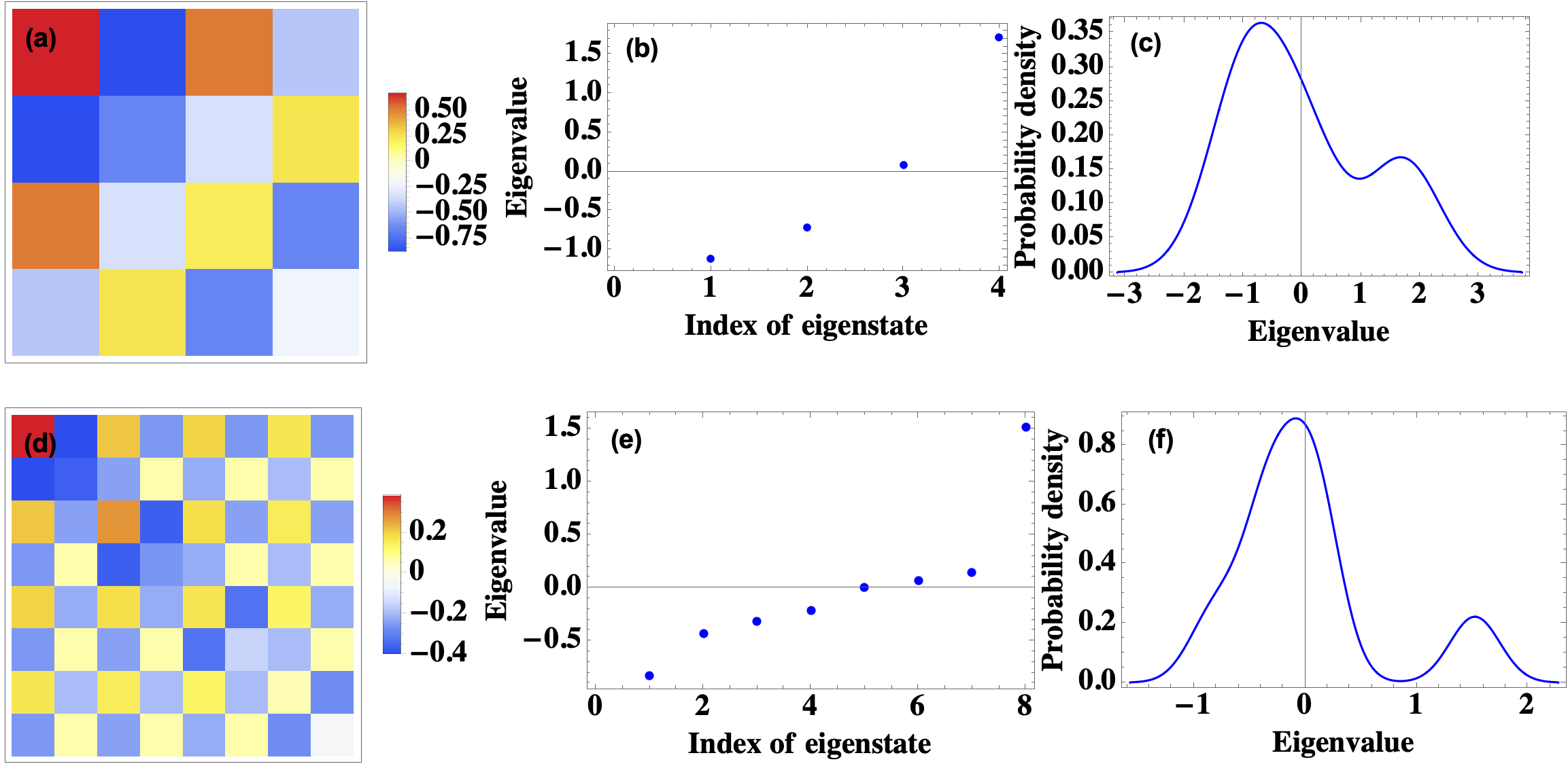
Figure 3: (a)-(c) show the results for $D=4$, where the entries distribution follows $\mathcal{N}(-0.193537,0.25)$. (d)-(f) show the results for $D=8$, where the distribution of elements of ${\bf H}$ follows $\mathcal{N}(-0.0916,0.04)$. Comparing to the method that identifying the parameters by considering the second the fourth moments of Gaussian variables $\psi_{m,i}$, as shown in Fig.2, the method that matching the diagonal elements of the corresponding singular matrix is more efficient. The eigenvalue distribution is also different from that in Fig.2 and Fig.1, where the probability density is larger for the negative eigenvalues, and this feature will more obvious for larger $D$. In this case, although the off-diagonal elements deviate from zero mean, but the variance $\overline{H_{mm^{\prime}}^{2}}-\overline{H_{mm^{\prime}}}^{2}=0.0400796$ as well as that for all elements of ${\bf H}$ ($\overline{H_{mm^{\prime}}^{2}}-\overline{H_{mm^{\prime}}}^{2}+\overline{H_{mm}^{2}}-\overline{H_{mm}}^{2}=0.0440813$) are close to the GOE predictions, which is $0.03125$ and $0.0351563$, respectively.

11 Appendx.B: Replica approach in solving $H_{\flat=2}\times H_{\flat=2}\times H_{\flat^{\prime}=1}$ Hamiltonian $H_{p}$

For small but finite $\Lambda_{q}$ case, the Hamiltonian $H_{p}$ describes a $H_{\flat=2}\times H_{\flat=2}\times H_{\flat^{\prime}=1}$ model,

$$H_{p}=g_{q}\sum_{i,j,k,l}\sum_{q}\Phi_{il}\Phi_{jk}c^{{\dagger}}_{i}c_{l}c^{{\dagger}}_{j}c_{k}.$$ (168)

The disorder average over $ijkl$ and $q$ will be done in the same time. Firstly, the Euclidean time path integral reads

$$Z= \int D[c^{{\dagger}},c]e^{-S},$$ (169)

$$S_{0}= \int d\tau d\tau^{\prime}[\sum_{i}^{N}c^{{\dagger}}_{i}(\tau)\partial_{\tau}\delta(\tau-\tau^{\prime})c_{i}(\tau^{\prime})],$$

$$S_{int}= \int d\tau d\tau^{\prime}[g_{q}\sum_{i,j,k,l}\sum_{q}\Phi_{il}\Phi_{jk}c^{{\dagger}}_{i}c_{l}c^{{\dagger}}_{j}c_{k}].$$

Using the replica trick $\overline{{\rm ln}Z}=\lim_{n\rightarrow 0}\frac{\overline{Z^{n}}-1}{n}$ the Gaussian average, we have

$$Z= \int D[c^{{\dagger}},c]\sum_{q}e^{-\int d\tau d\tau^{\prime}[c^{{\dagger}}_{i}(\tau)\partial_{\tau}\delta(\tau-\tau^{\prime})c_{i}(\tau)+g_{q}^{-1}b_{1}^{-q}b_{2}^{q}]}\int D[\Phi_{il},\Phi_{il}^{*}]\sum_{q}e^{-\frac{|\Phi^{-q}_{il}|^{2}}{\sigma^{2}}}$$ (170)

$$\int D[\Phi_{jk},\Phi_{jk}^{*}]\sum_{q}e^{-\frac{|\Phi^{q}_{jk}|^{2}}{\sigma^{2}}}$$

$$\int D[\Phi_{il},\Phi_{il}^{*}]\int D[\Phi_{jk},\Phi_{jk}^{*}]\sum_{q}e^{-\int d\tau d\tau^{\prime}(i\Phi^{-q}_{il}c^{{\dagger}}_{i}c_{l}b_{1}^{-q}+i\Phi^{-q}_{jk}c^{{\dagger}}_{j}c_{k}b_{2}^{q}+H.c.)}.$$

where $\sigma^{2}=\overline{\Phi_{ik}^{2}}$ is the variance of Gaussian variable $\Phi_{ik}$, and $D[\Phi_{il},\Phi_{il}^{*}]=\prod_{il}d\Phi_{il}d\Phi_{il}^{*}$, $D[\Phi_{jk},\Phi_{jk}^{*}]=\prod_{jk}d\Phi_{jk}d\Phi_{jk}^{*}$, $D[c_{i}^{{\dagger}},c_{i}]=\prod_{i}dc^{{\dagger}}_{i}dc_{i}$. Note that here within the Gaussian average, the Gaussian distribution should be $e^{-\frac{|\Phi_{jk}|^{2}}{\sigma^{2}}}$ insteads of $e^{-\frac{|\Phi_{jk}|^{2}}{2\sigma^{2}}}$, because the factor 2 in the denominator has in fact already been considered in the replia process by observable $\mathcal{O}$. Here $\sigma^{2}=\overline{\Phi_{il}^{2}}=\frac{J}{2N}2\Lambda_{q}=\frac{J}{N}\Lambda_{q}$. And here we use the identity

$$\int D[a]e^{-ga_{1}a_{2}\cdot\cdot\cdot a_{n}}=\int D[a]\int D[b]e^{-g^{-1}b_{1}b_{2}\cdot\cdot\cdot b_{n}-i\sum_{\alpha=1}^{n}b_{\alpha}a_{\alpha}},$$ (171)

to decouple the two Gaussian variables. This relys on the identity

$$\int D[b]e^{-g^{-1}(b+iag)^{n}}=1.$$ (172)

Since

$$\int d\Phi_{il}d\Phi_{il}^{*}e^{-\frac{|\Phi_{il}|^{2}}{\sigma^{2}}}e^{-(i\Phi^{-q}_{il}c^{{\dagger}}_{i}c_{l}b_{1}^{-q}+H.c.)}=\int d\Phi_{il}d\Phi_{il}^{*}e^{-\frac{|\Phi_{il}|^{2}}{\sigma^{2}}}e^{-(i\Phi^{-q}_{il}c^{{\dagger}}_{i}c_{l}b_{1}^{-q}-i\Phi^{-q*}_{il}c^{{\dagger}}_{l}c_{i}b^{-q*}_{1})}$$ (173)

$$=\int d\Phi_{il}d\Phi_{il}^{*}e^{\frac{-1}{\sigma^{2}}(\Phi_{il}^{-q}-i\sigma^{2}c^{{\dagger}}_{l}c_{i}b_{1}^{-q*})(\Phi_{il}^{-q*}+i\sigma^{2}c^{{\dagger}}_{i}c_{l}b_{1}^{-q})}e^{\sigma^{2}(b_{1}^{-q}c_{i}^{{\dagger}}c_{l})(b_{1}^{-q}c_{i}^{{\dagger}}c_{l})^{*}}$$

$$=e^{\sigma^{2}(b_{1}^{-q}c_{i}^{{\dagger}}c_{l})(b_{1}^{-q}c_{i}^{{\dagger}}c_{l})^{*}},$$

similarly,

$$\int d\Phi_{jk}d\Phi_{jk}^{*}e^{-\frac{|\Phi_{jk}|^{2}}{\sigma^{2}}}e^{-(i\Phi^{q}_{jk}c^{{\dagger}}_{j}c_{k}b_{2}^{q}+H.c.)}=e^{\sigma^{2}(b_{2}^{q}c_{j}^{{\dagger}}c_{k})(b_{2}^{q}c_{j}^{{\dagger}}c_{k})^{*}}.$$ (174)

then the action can be written as

$$S= \int d\tau d\tau^{\prime}[\sum_{i}c^{{\dagger}}_{i}(\tau)\partial_{\tau}\delta(\tau-\tau^{\prime})c_{i}(\tau)+\sum_{q}g_{q}^{-1}b_{1*}^{-q}(\tau)b_{2}^{q}(\tau^{\prime})+\sum_{q}g_{q}^{-1}b_{2*}^{q}(\tau)b_{1}^{-q}(\tau^{\prime})]$$ (175)

$$-\int d\tau d\tau^{\prime}\sum_{q}\sigma^{2}(b_{1}^{-q}c_{i}^{{\dagger}}c_{l})(b_{1}^{-q}c_{i}^{{\dagger}}c_{l})^{*}-\int d\tau d\tau^{\prime}\sum_{q}\sigma^{2}(b_{2}^{q}c_{j}^{{\dagger}}c_{k})(b_{2}^{q}c_{j}^{{\dagger}}c_{k})^{*}$$

$$= \int d\tau d\tau^{\prime}[\sum_{i}c^{{\dagger}}_{i}(\tau)\partial_{\tau}\delta(\tau-\tau^{\prime})c_{i}(\tau)+\sum_{q}g_{q}^{-1}b_{1}^{-q}(\tau)b_{2}^{q}(\tau^{\prime})]$$

$$-\int d\tau d\tau^{\prime}\sum_{q}\frac{J\Lambda_{q}}{N}(b_{1}^{-q}c_{i}^{{\dagger}}c_{l})(b_{1}^{-q}c_{i}^{{\dagger}}c_{l})^{*}-\int d\tau d\tau^{\prime}\sum_{q}\frac{J\Lambda_{q}}{N}(b_{2}^{q}c_{j}^{{\dagger}}c_{k})(b_{2}^{q}c_{j}^{{\dagger}}c_{k})^{*}.$$

By inserting the identities (in mean-field approximation with $N\rightarrow\infty$)

$$1= \int DG_{f}\delta[G_{f}(\tau^{\prime},\tau)-\frac{1}{N}\sum_{i}c_{i}^{{\dagger}}(\tau)c_{i}(\tau^{\prime})]$$ (176)

$$= \int DG_{f}\delta[NG_{f}(\tau^{\prime},\tau)-\sum_{i}c_{i}^{{\dagger}}(\tau)c_{i}(\tau^{\prime})]$$

$$= \int DG_{f}D\Sigma{\rm exp}[N\Sigma(\tau,\tau^{\prime})G_{f}(\tau^{\prime},\tau)-\Sigma(\tau,\tau^{\prime})\sum_{i}c_{i}^{{\dagger}}(\tau)c_{i}(\tau^{\prime})],$$

$$1= \int D\mathcal{D}D\Pi{\rm exp}[\Lambda_{q}^{-1}\Pi(\tau,\tau^{\prime})D(\tau^{\prime},\tau)-\Pi(\tau,\tau^{\prime})\sum_{q}b_{1}^{-q*}(\tau)b_{1}^{-q}(\tau^{\prime})],$$

$$1= \int D\mathcal{D}^{\prime}D\Pi^{\prime}{\rm exp}[\Lambda_{q}^{-1}\Pi^{\prime}(\tau,\tau^{\prime})D^{\prime}(\tau^{\prime},\tau)-\Pi^{\prime}(\tau,\tau^{\prime})\sum_{q}b_{2}^{q*}(\tau)b_{2}^{q}(\tau^{\prime})],$$

and the Green's functions

$$\mathcal{D}(\tau,\tau^{\prime})=\Lambda_{q}\sum_{q}b_{1}^{-q*}(\tau^{\prime})b_{1}^{-q}(\tau),$$ (177)

$$\mathcal{D}^{\prime}(\tau,\tau^{\prime})=\Lambda_{q}\sum_{q}b_{2}^{q*}(\tau^{\prime})b_{2}^{q}(\tau),$$

$$G_{f}(\tau,\tau^{\prime})=\frac{1}{N}\sum_{i}c_{i}^{{\dagger}}(\tau^{\prime})c_{i}(\tau),$$

we obtain

$$S= -N\int d\tau d\tau^{\prime}{\rm Tr}{\rm ln}[\partial_{\tau}+\Sigma(\tau,\tau^{\prime})]+\sum_{q}g_{q}^{-1}b_{1}^{-q}(\tau)b_{2}^{q*}(\tau^{\prime})+\sum_{q}g_{q}^{-1}b_{2}^{q}(\tau)b_{1}^{-q*}(\tau^{\prime})]$$ (178)

$$-N\int d\tau d\tau^{\prime}J(-\mathcal{D}(\tau,\tau^{\prime}))G_{f}^{2}(\tau,\tau^{\prime})-N\int d\tau d\tau^{\prime}J(-\mathcal{D}^{\prime}(\tau,\tau^{\prime}))G_{f}^{2}(\tau,\tau^{\prime})$$

$$-\int d\tau d\tau^{\prime}[\Lambda_{q}^{-1}\Pi(\tau,\tau^{\prime})b_{1}^{-q}(\tau)b_{1}^{-q*}(\tau^{\prime})+\Lambda_{q}^{-1}\Pi^{\prime}(\tau^{\prime},\tau)b_{2}^{q}(\tau)b_{2}^{q*}(\tau^{\prime})]$$

$$-\int d\tau d\tau^{\prime}\Lambda_{q}^{-1}\Pi(\tau,\tau^{\prime})\mathcal{D}(\tau^{\prime},\tau)-\int d\tau d\tau^{\prime}\Lambda_{q}^{-1}\Pi^{\prime}(\tau,\tau^{\prime})\mathcal{D}^{\prime}(\tau^{\prime},\tau)-\int d\tau d\tau^{\prime}N\Sigma(\tau,\tau^{\prime})G_{f}(\tau^{\prime},\tau)$$

$$= -N\int d\tau d\tau^{\prime}{\rm Tr}{\rm ln}[\partial_{\tau}+\Sigma(\tau,\tau^{\prime})]-\Lambda_{q}^{-1}\int d\tau d\tau^{\prime}\begin{pmatrix}b_{1}^{-q}&b_{2}^{q}\end{pmatrix}\begin{pmatrix}\Pi(\tau,\tau^{\prime})&g_{q}^{-1}\\ (g_{q}^{-1})^{*}&\Pi^{\prime}(\tau,\tau^{\prime})\end{pmatrix}\begin{pmatrix}b_{1}^{-q*}\\ b_{2}^{q*}\end{pmatrix}$$

$$-N\int d\tau d\tau^{\prime}J(-\mathcal{D}(\tau,\tau^{\prime}))G_{f}^{2}(\tau,\tau^{\prime})-N\int d\tau d\tau^{\prime}J(-\mathcal{D}^{\prime}(\tau,\tau^{\prime}))G_{f}^{2}(\tau,\tau^{\prime})$$

$$-\int d\tau d\tau^{\prime}\Lambda_{q}^{-1}\Pi(\tau,\tau^{\prime})\mathcal{D}(\tau^{\prime},\tau)-\int d\tau d\tau^{\prime}\Lambda_{q}^{-1}\Pi^{\prime}(\tau,\tau^{\prime})\mathcal{D}^{\prime}(\tau^{\prime},\tau)-\int d\tau d\tau^{\prime}N\Sigma(\tau,\tau^{\prime})G_{f}(\tau^{\prime},\tau)],$$

in the case of particle-hole symmetry. Since the action depends neither on the time or frequency, i.e., $S=\int d\tau S(\tau)=T\sum_{\omega}S(\omega)$ and without need to introduce the exponentiall part, we can simply rewrite it in the frequency representation. Then using the saddle-point equations, we obtain

$$\frac{\partial S}{\partial\Sigma(\omega)} =-NG_{f}(\omega)-\frac{N}{-i\omega+\Sigma(\omega)}=0,$$ (179)

$$\frac{\partial S}{\partial G_{f}(\omega)} =-N\Sigma(\omega)-NJ(-\mathcal{D}(\omega))G_{f}(\omega)-NJ(-\mathcal{D}^{\prime}(\omega)G_{f}(\omega))=0,$$

$$\frac{\partial S}{\partial\Pi(\omega)} =-\Lambda_{q}^{-q}\mathcal{D}(\omega)-\frac{\Lambda_{q}^{-1}\Pi^{\prime}(\omega)}{\Pi(\omega)\Pi^{\prime}(\omega)-g_{q}^{-2}}=0,$$

$$\frac{\partial S}{\partial\mathcal{D}(\omega)} =-\Lambda_{q}^{-1}\Pi(\omega)-NJG_{f}^{2}(\omega)=0,$$

thus (at saddle-point $\mathcal{D}=\mathcal{D}^{\prime}$)

$$G_{f}(\omega)= -\frac{1}{\partial_{\tau}+\Sigma(\omega)},$$ (180)

$$\Sigma(\omega)= J\mathcal{D}(\omega)G_{f}(\omega)+J\mathcal{D}^{\prime}(\omega)G_{f}(\omega),$$

$$\mathcal{D}(\omega)= -\frac{\Pi^{\prime}(\omega)}{\Pi(\omega)\Pi^{\prime}(\omega)-g_{q}^{-2}},$$

$$\Pi(\omega)= -N\Lambda_{q}JG_{f}^{2}(\omega).$$

This conformal saddle-point is stable when $N\sim\Lambda_{q}^{-1}$. And then the fermion Green's function can be obtained by solving

$$i\omega N^{2}\Lambda_{q}^{2}J^{2}G_{f}^{5}(\omega)-i\omega G_{f}(\omega)g^{-2}_{q}-2N\Lambda_{q}J^{2}G_{f}^{4}-N^{2}\Lambda_{q}^{2}J^{2}G_{f}^{4}+g_{q}^{-2}=0.$$ (181)

In IR limit, we obtain the random matrix solutions

$$G_{f}=\frac{\pm 1}{(J^{4}\Lambda_{q}N(2+\Lambda_{q}N))^{1/4}},\frac{\pm i}{(J^{4}\Lambda_{q}N(2+\Lambda_{q}N))^{1/4}}.$$ (182)

The self-energy can also be obtained and they satisfy

$$G_{f}\Sigma=-1.$$ (183)

We are unable to recognize the fermi-liquid or non-fermi liquid behaviors from the frequency-dependence base on this IR solution, but we can recognize it through the discussion of scale invariance. For Eq.(175) under the scaling $\tau\rightarrow B\tau$, to keep the $J$-dependent term be invariant, we have $c\rightarrow B^{-1/4}c$, $b\rightarrow B^{-1/2}b$, thus the fermions have a scaling dimension $1/4$, i.e., they follows the $H_{\flat=4}$ non-fermi liquid behavior. But this requires $\mathcal{D}$ be a boson propagator, with $b=cc$. This result will be further verified in the Appendix.C, where the retarded form the Green's function and the spectral density are derived with a frequency-dependence.

The SYK behavior can also be seem from the diagrammatic representation of self-energy in conformal saddle-point, as shown in Fig.3, which is equivalents to that of $H_{\flat=4}$ systems[4, 26]: three dressed fermion propagators and an interaction contraction.

Then the free energy density can be obtained as

$$f= \frac{F}{N\Lambda_{q}^{-1}}=\frac{-T{\rm ln}Z}{N\Lambda_{q}^{-1}}$$ (184)

$$= -\frac{T}{N\Lambda_{q}^{-1}}(N\sum_{\omega}{\rm ln}(-\beta g^{-1}(i\omega))+\Lambda_{q}^{-1}\sum_{\omega}{\rm det}(-\beta\mathcal{D}^{-1}(i\omega))$$

$$-\frac{1}{N\Lambda_{q}^{-1}}\int^{\beta}_{0}d\tau(NJg^{2}(\tau)\mathcal{D}(-\tau)+NJg^{2}(\tau)\mathcal{D}^{\prime}(-\tau)),$$

where

$$g(i\omega)= \frac{1}{i\omega-\Sigma(i\omega)},$$ (185)

$$g_{B}^{-1}(i\omega)= -\begin{pmatrix}\Pi(\tau,\tau^{\prime})&g_{q}^{-1}\\ g_{q}^{-1}&\Pi^{\prime}(\tau,\tau^{\prime})\end{pmatrix},$$

$$g_{B}(i\omega)= -\frac{1}{|\Pi(\tau,\tau^{\prime})\Pi^{\prime}(\tau,\tau^{\prime})-g_{q}^{-2}|}\begin{pmatrix}\Pi^{\prime}(\tau,\tau^{\prime})&-g_{q}^{-1}\\ -g_{q}^{-1}&\Pi(\tau,\tau^{\prime})\end{pmatrix}.$$

For first term we have

$$\sum_{\omega}{\rm ln}(-\beta g^{-1}(i\omega))e^{i\omega 0^{+}}= \sum_{\omega}{\rm ln}(-\beta g^{-1}_{0}(i\omega))e^{i\omega 0^{+}}+\sum_{\omega}{\rm ln}\frac{-\beta g^{-1}(i\omega)}{-\beta g^{-1}_{0}(i\omega)}e^{i\omega 0^{+}}$$ (186)

$$= {\rm ln}2+\sum_{\omega}{\rm ln}(1-\frac{-\int^{\beta}_{0}d\tau e^{i\omega\tau}\frac{J}{2}\mathcal{D}(\tau,\tau^{\prime})G_{f}(\tau^{\prime},\tau)}{i\omega})e^{i\omega 0^{+}},$$

since at saddle point $\mathcal{D}=\mathcal{D}^{\prime}$. The second term reads

$$\sum_{\omega}{\rm det}(-\beta g_{B}^{-1}(i\omega))= \beta^{2}(\Pi^{2}(i\omega)-g_{q}^{-2})$$ (187)

$$= \sum_{\omega}\beta^{2}(\Pi^{2}(i\omega)+(ig_{q}^{-1})^{2}).$$

Note that we do not consider the spin degree-of-freedom in this Appendix. If the spin degree-of-freedom is considered, we only need to replace the deviation $\sigma^{2}=\overline{\Phi_{il}^{2}}=\frac{J\Lambda_{q}}{N}$ by the $\sigma^{2}=\overline{\Phi_{il\sigma}^{2}}=\frac{J\Lambda_{q}}{2N}$.

12 Appendix.C: Fermion density calculation base on Luttinger-Ward analysis

The fermion density at zero temperature can be calculated through

$$n^{\prime}=G(\tau^{\prime},\tau)=G(0^{+})= \mathcal{Q}-\frac{1}{2}$$ (188)

$$= \int^{i\infty}_{-\infty}\frac{dz}{2\pi i}g(z)e^{z0^{-}},$$

where $\mathcal{Q}$ denotes the U(1) charge, and $n^{\prime}=-1+n$ with $n=G(\tau,\tau^{\prime})=G(0^{-})=\mathcal{Q}+\frac{1}{2}$. Using the identity $\partial_{z}(g^{-1}(z)+\Sigma(z))=1$, we have

$$n^{\prime}= \int^{i\infty}_{-i\infty}\frac{dz}{2\pi i}g(z)\partial_{z}(g^{-1}(z)+\Sigma(z))e^{z0^{-}}$$ (189)

$$= P\int^{i\infty}_{-i\infty}\frac{dz}{2\pi i}g(z)\partial_{z}g^{-1}(z)e^{z0^{-}}+P\int^{i\infty}_{-i\infty}\frac{dz}{2\pi i}g(z)\partial_{z}\Sigma(z)e^{z0^{-}}$$

$$\equiv I_{1}+I_{2},$$

where we define $P\int^{i\infty}_{-i\infty}=\int^{i\infty}_{i\eta}+\int^{-i\eta}_{-i\infty}=\int^{\infty+i\eta}_{i\eta}-\int^{\infty-i\eta}_{-i\eta}=\int^{-\infty+i\eta}_{i\eta}-\int^{-\infty-i\eta}_{-i\eta}$ to carry out the principal value integral along the contour,, and we define the phase shift as

$$\delta=\frac{i}{2}{\rm ln}\frac{g(z+i\eta)}{g(z-i\eta)}=\frac{1}{-i}{\rm ln}\frac{g(z+i\eta)}{g(z)}=\frac{1}{i}{\rm ln}\frac{g(z-i\eta)}{g(z)}=-{\rm Arg}g(z+i\eta),$$ (190)

which equivalents to the relation $\frac{g(z+i\eta)}{g(z-i\eta)}=e^{2i{\rm Arg}g(z+i\eta)}$.

The integral in the first term ($I_{1}$) can be rewritten as

$$I_{1}= -P\int^{i\infty}_{-i\infty}\frac{dz}{2\pi i}g^{-1}(z)\partial_{z}g(z)e^{z0^{-}}$$ (191)

$$= -P\int^{i\infty}_{-i\infty}\frac{dz}{2\pi i}\partial_{z}{\rm ln}g(z)e^{z0^{-}}$$

$$= -(\int^{\infty+i\eta}_{0+i\eta}-\int^{\infty-i\eta}_{0-i\eta})\frac{dz}{2\pi i}\partial_{z}{\rm ln}g(z)e^{z0^{-}}$$

$$= -\int^{\infty}_{0}\frac{dz}{2\pi i}\partial_{z}{\rm ln}\frac{g(z+i\eta)}{g(z-i\eta)}e^{z0^{-}}$$

$$= -\frac{1}{\pi}({\rm Arg}g(\infty+i\eta)-{\rm Arg}g(i\eta))$$

$$= -\frac{1}{2}-\frac{\theta}{\pi},$$

where ${\rm Arg}g(\infty+i\eta)=0$, ${\rm Arg}g(0+i\eta)=-\frac{\pi}{2}-\theta$.

The above result can also be obtained by

$$I_{1}= -P\int^{i\infty}_{-i\infty}\frac{dz}{2\pi i}\partial_{z}{\rm ln}g(z)e^{z0^{-}}$$ (192)

$$= -P\int^{\infty}_{0}\frac{dz}{2\pi i}\partial_{z}{\rm ln}g(z+i\eta)e^{z0^{-}}-P\int^{0}_{-\infty}\frac{dz}{2\pi i}\partial_{z}{\rm ln}g(z-i\eta)e^{z0^{-}}$$

$$= -P\int^{\infty}_{-\infty}\frac{dz}{2\pi i}\partial_{z}{\rm ln}g(z+i\eta)e^{z0^{-}}-P\int^{0}_{-\infty}\frac{dz}{2\pi i}\partial_{z}{\rm ln}\frac{g(z-i\eta)}{g(z+i\eta)}e^{z0^{-}}=-1+(\frac{1}{2}-\frac{\theta}{\pi})=-\frac{1}{2}-\frac{\theta}{\pi},$$

where ${\rm ln}\frac{g(z-i\eta)}{g(z+i\eta)}=-2i{\rm Arg}g(z+i\eta)$, and

$$-P\int^{\infty}_{-\infty}\frac{dz}{2\pi i}\partial_{z}{\rm ln}g(z+i\eta)e^{z0^{-}}=-1.$$ (193)

Similarly,

$$I_{1}= -P\int^{\infty}_{0}\frac{dz}{2\pi i}\partial_{z}{\rm ln}\frac{g(z+i\eta)}{g(z-i\eta)}e^{z0^{-}}-P\int^{\infty}_{-\infty}\frac{dz}{2\pi i}\partial_{z}{\rm ln}g(z-i\eta)e^{z0^{-}}$$ (194)

$$= -\frac{1}{2}-\frac{\theta}{\pi}-0=-\frac{1}{2}-\frac{\theta}{\pi},$$

where ${\rm ln}\frac{g(z-i\eta)}{g(z+i\eta)}=2i{\rm Arg}g(z+i\eta)$, and

$$-P\int^{\infty}_{0}\frac{dz}{2\pi i}\partial_{z}{\rm ln}\frac{g(z+i\eta)}{g(z-i\eta)}e^{z0^{-}}=0.$$ (195)

The above expressions of $I_{1}$ can be verified by

$$P\int^{\infty}_{-\infty}\frac{dz}{2\pi i}\partial_{z}{\rm ln}\frac{g(z+i\eta)}{g(z-i\eta)}e^{z0^{-}}=1.$$ (196)

Then we turn to equation $I_{2}$

$$I_{2}= P\int^{i\infty}_{-i\infty}\frac{dz}{2\pi i}g(z)\partial_{z}\Sigma(z)e^{z0^{-}}.$$ (197)

According to above section and Appendix.B, the self-energy is

$$\Sigma(\tau)\sim D_{1}(\tau)g(-\tau)+D_{2}(\tau)g(-\tau),$$ (198)

where $D$ and $g$ denote the boson and fermion Green's function, respectively. In frequency domain the self-energy reads

$$\Sigma(z)= -\int\frac{d\Omega^{\prime}}{2\pi}\int\frac{d\Omega_{1}}{2\pi}\int^{\infty}_{-\infty}\frac{d\nu}{2\pi}\frac{\rho_{B}(\Omega_{1})}{i\Omega^{\prime}-\Omega_{1}}\frac{\rho_{F}(\nu)}{Z-i\Omega^{\prime}-\nu}+(\Omega_{1}\leftrightarrow\Omega_{2})$$ (199)

$$= \int^{\infty}_{-\infty}\frac{d\Omega_{1}}{2\pi}\int^{\infty}_{-\infty}\frac{d\nu}{2\pi}\frac{\rho_{B}(\Omega_{1})\rho_{F}(\nu)}{Z-\Omega_{1}-\nu}({\rm sgn}[\Omega_{1}]+{\rm sgn}[\nu])+(\Omega_{1}\leftrightarrow\Omega_{2}),$$

where $\rho_{B}$ and $\rho_{F}$ denote the boson and fermion spectral function, respectively, and it requires ${\rm sgn}[\Omega]={\rm sgn}[\nu]$. Thus $I_{2}$ can be rewritten as

$$I_{2}= P\int^{i\infty}_{-i\infty}\frac{dz}{2\pi i}e^{z0^{-}}\int\frac{d\omega}{2\pi}\frac{\rho_{F}(\omega)}{z-\omega}\int\frac{d\Omega_{1}}{2\pi}\int^{\infty}_{-\infty}\frac{d\nu}{2\pi}\frac{\rho_{B}(\Omega_{1})\rho_{F}(\nu)}{(z-\Omega_{1}-\nu)^{2}}({\rm sgn}[\Omega_{1}]+{\rm sgn}[\nu])+(\Omega_{1}\leftrightarrow\Omega_{2}).$$ (200)

This expression is equivalent to

$$I_{2}= P\int^{-i\infty}_{i\infty}\frac{d(-z)}{2\pi i}e^{-z0^{-}}\int^{-\infty}_{\infty}\frac{d(-\omega)}{2\pi}\frac{\rho_{F}(-\omega)}{-z+\omega}$$ (201)

$$\int^{-\infty}_{\infty}\frac{d(-\Omega_{1})}{2\pi}\int^{-\infty}_{\infty}\frac{d(-\nu)}{2\pi}\frac{\rho_{B}(-\Omega_{1})\rho_{F}(-\nu)}{(-z+\Omega_{1}+\nu)^{2}}(-{\rm sgn}[\Omega_{1}]-{\rm sgn}[\nu])+(\Omega_{1}\leftrightarrow\Omega_{2})$$

$$= P\int^{i\infty}_{-i\infty}\frac{dz}{2\pi i}e^{-z0^{-}}\int^{\infty}_{-\infty}\frac{d\omega}{2\pi}\frac{\rho_{F}(-\omega)}{z-\omega}$$

$$\int^{\infty}_{-\infty}\frac{d\Omega_{1}}{2\pi}\int^{\infty}_{-\infty}\frac{d\nu}{2\pi}\frac{\rho_{B}(-\Omega_{1})\rho_{F}(-\nu)}{(z-\Omega_{1}-\nu)^{2}}({\rm sgn}[\Omega_{1}]+{\rm sgn}[\nu])+(\Omega_{1}\leftrightarrow\Omega_{2}).$$

This can also be written as

$$I_{2}= -P\int^{i\infty}_{-i\infty}\frac{dz}{2\pi i}e^{-z0^{-}}\int^{\infty}_{-\infty}\frac{d\omega}{2\pi}\frac{\rho_{F}(\omega)}{-z-\omega}$$ (202)

$$\int^{\infty}_{-\infty}\frac{d\Omega_{1}}{2\pi}\int^{\infty}_{-\infty}\frac{d\nu}{2\pi}\frac{\rho_{B}(-\Omega_{1})\rho_{F}(-\nu)}{(z-\Omega_{1}-\nu)^{2}}({\rm sgn}[\Omega_{1}]+{\rm sgn}[\nu])+(\Omega_{1}\leftrightarrow\Omega_{2})$$

$$= P\int^{i\infty}_{-i\infty}\frac{dz}{2\pi i}e^{-z0^{-}}\int^{\infty}_{-\infty}\frac{d\omega}{2\pi}\frac{\rho_{F}(\omega)}{z+\omega}$$

$$\int^{\infty}_{-\infty}\frac{d\Omega_{1}}{2\pi}\int^{\infty}_{-\infty}\frac{d\nu}{2\pi}\frac{\rho_{B}(-\Omega_{1})\rho_{F}(-\nu)}{(z-\Omega_{1}-\nu)^{2}}({\rm sgn}[\Omega_{1}]+{\rm sgn}[\nu])+(\Omega_{1}\leftrightarrow\Omega_{2}),$$

or

$$I_{2}= P\int^{i\infty}_{-i\infty}\frac{dz}{2\pi i}e^{z0^{-}}\int^{\infty}_{-\infty}\frac{d\omega}{2\pi}\frac{\rho_{F}(-\omega)}{z+\omega}$$ (203)

$$\int^{\infty}_{-\infty}\frac{d\Omega_{1}}{2\pi}\int^{\infty}_{-\infty}\frac{d\nu}{2\pi}\frac{\rho_{B}(\Omega_{1})\rho_{F}(\nu)}{(z-\Omega_{1}-\nu)^{2}}({\rm sgn}[\Omega_{1}]+{\rm sgn}[\nu])+(\Omega_{1}\leftrightarrow\Omega_{2}).$$

According to the above four equations, we have

$$I_{2}= \frac{1}{4}(2I_{2}+2I_{2})$$ (204)

$$= \frac{1}{4}[P\int^{i\infty}_{-i\infty}\frac{dz}{2\pi i}e^{z0^{-}}\int^{\infty}_{-\infty}\frac{d\omega}{2\pi}$$

$$\int^{\infty}_{-\infty}\frac{d\Omega_{1}}{2\pi}\int^{\infty}_{-\infty}\frac{d\nu}{2\pi}\frac{\rho_{F}(\omega)\rho_{B}(\Omega_{1})\rho_{F}(\nu)+\rho_{F}(-\omega)\rho_{B}(-\Omega_{1})\rho_{F}(-\nu)}{(z-\omega)(z-\Omega_{1}-\nu)^{2}}({\rm sgn}[\Omega_{1}]+{\rm sgn}[\nu])+(\Omega_{1}\leftrightarrow\Omega_{2})]$$

$$+\frac{1}{4}[P\int^{i\infty}_{-i\infty}\frac{dz}{2\pi i}e^{z0^{-}}\int^{\infty}_{-\infty}\frac{d\omega}{2\pi}\int^{\infty}_{-\infty}\frac{d\Omega_{1}}{2\pi}\int^{\infty}_{-\infty}\frac{d\nu}{2\pi}$$

$$\frac{\rho_{F}(\omega)\rho_{B}(-\Omega_{1})\rho_{F}(-\nu)+\rho_{F}(-\omega)\rho_{B}(\Omega_{1})\rho_{F}(\nu)}{(z+\omega)(z-\Omega_{1}-\nu)^{2}}({\rm sgn}[\Omega_{1}]+{\rm sgn}[\nu])+(\Omega_{1}\leftrightarrow\Omega_{2})].$$

To further process, we need to know the detail form of spectral functions as well as the conformal solutions of the corresponding Green's function. According to Eq.180, by rewriting the boson operators as

$$b^{-q}_{1}(\tau)= c_{1}^{{\dagger}}(\tau)c_{1}(\tau),$$ (205)

$$b^{q}_{2}(\tau)= c_{2}^{{\dagger}}(\tau)c_{2}(\tau),$$

we found the self-energy $\Sigma(\tau)\sim-Jg^{2}(\tau)g(-\tau)$, which is the same as the self-energy of $H_{\flat=4}$ model. Thus the self-energy (as well as Green's function in conformal limit) of $H_{\flat=2}\times$$H_{\flat=2}$ model is equivalence to the $H_{\flat=4}$ model except the SYK coupling constant. This relys on the construction of auxiliary boson propagator during the decoupling procedure, and it is not an universally result, e.g., the self-energy (as well as Green's function in conformal limit) of $H_{\flat=4}\times$$H_{\flat=4}$ model will not the same with the $H_{\flat=8}$ model.

Then the imaginary time Green's function in low temperature limit ($\omega>\beta$) has the form

$$g(\tau)\sim\sqrt{\frac{T}{{\rm sin}\pi T\tau}},$$ (206)

instead of the Fermi liquid form which is

$$g_{FL}(\tau)\sim\frac{T}{{\rm sin}\pi T\tau}.$$ (207)

Also, the density-of-states in fermi liquid phase is indepedent of frequency, while the density-of-states is indepedent of frequency only in zero eigenvalue.

In zero temperature limit, we write the retarded Green's functions and the corresponding self-energy as

$$g_{R}(\omega)= C\frac{e^{-i(\pi/4+\theta)}}{\omega^{1/2}J^{1/4}2^{-1/2}},$$ (208)

$$\Sigma_{R}(\omega)= \frac{-e^{i(\pi/4+\theta)}}{C\omega^{-1/2}J^{-1/4}2^{1/2}}.$$

For large $\Lambda_{q}^{-1}$, which corresponds to large $g_{q}$, the boson propagator can be written as

$$D_{R}(\omega)\approx \frac{-1}{\Pi(\omega)}$$ (209)

$$= -(N\Lambda_{q}JG_{f}^{2}(\omega))^{-1}$$

$$= -\frac{\omega e^{2i(\pi/4+\theta)}}{N\Lambda_{q}J^{1/2}C^{2}2}.$$

Then the spectral functiosn read

$$\rho_{F}(\omega)= -{\rm Im}g(\omega+i\eta),$$ (210)

$$\rho_{B}(\omega)= {\rm Im}D(\omega+i\eta).$$

In the above equation, the parameter $C$ is related to the spetral asymmetry and is positive as long as the spectral function is positive. By solving this we obtain

$$\rho_{F}(\pm\omega)= \frac{\sqrt{2}C{\rm sin}[\frac{1}{4}(\pi+4\theta+{\rm Arg}[J]+2{\rm Arg}[i\eta\pm\omega])]}{J^{1/4}(\eta^{2}+\omega^{2})^{1/4}},$$ (211)

$$\rho_{B}(\pm\omega)= \frac{4C^{4}J\Lambda_{q}^{2}N^{2}(\mp 2\eta\omega{\rm cos}[4\theta]+(\eta^{2}-\omega^{2}){\rm sin}[4\theta])}{(\eta^{2}+\omega^{2})^{2}},$$

where ${\rm Arg}[J]=\pi$ since $J<0$, and ${\rm Arg}(\omega+i\eta)=-\theta-\frac{\pi}{4}$, ${\rm Arg}(-\omega+i\eta)=-\theta-\frac{3\pi}{4}$ in the IR limit where we let $\omega\rightarrow 0^{+}\approx\eta$. Then the spectral functions can be rewritten as

$$\rho_{F}(\pm\omega)= \rho_{F1}(\omega)\rho_{F0}({\rm sgn}[\omega])$$ (212)

$$= \frac{\sqrt{2}C{\rm sin}[\frac{\pi}{2}+\frac{\theta}{2}-\frac{\pi}{8}]}{J^{1/4}(\eta^{2}+\omega^{2})^{1/4}}\rho_{F0}({\rm sgn}[\omega]),$$

$$\rho_{B}(\pm\omega)\approx \frac{4C^{4}J\Lambda_{q}^{2}N^{2}(\mp 2\eta\omega{\rm cos}[4\theta])}{(\eta^{2}+\omega^{2})^{2}}$$

$$= \rho_{B1}(\omega)\rho_{B0}({\rm sgn}[\omega])$$

$$= \frac{4C^{4}J\Lambda_{q}^{2}N^{2}\omega}{(\eta^{2}+\omega^{2})^{2}}\rho_{B0}({\rm sgn}[\omega]),$$

where

$$\rho_{F0}({\rm sgn}[\omega])= \begin{cases}1,&{\rm sgn}[\omega]=+,\\ \frac{1}{\sqrt{2}}-\frac{{\rm cot}[\frac{\pi}{2}+\frac{\theta}{2}-\frac{\pi}{8}]}{\sqrt{2}},&{\rm sgn}[\omega]=-,\\ \end{cases}\rho_{B0}({\rm sgn}[\omega])= -{\rm sgn}[\omega]2\eta{\rm cos}[4\theta].$$ (213)

Thus $\rho_{B}(-\Omega)=-\rho_{B}(\Omega)$, and $I_{2}$ can be rewritten as

$$I_{2}= \frac{1}{4}(2I_{2}+2I_{2})$$ (214)

$$= \frac{1}{4}[P\int^{i\infty}_{-i\infty}\frac{dz}{2\pi i}e^{z0^{-}}\int^{\infty}_{-\infty}\frac{d\omega}{2\pi}$$

$$\int^{\infty}_{-\infty}\frac{d\Omega_{1}}{2\pi}\int^{\infty}_{-\infty}\frac{d\nu}{2\pi}\frac{\rho_{B}(\Omega_{1})(\rho_{F}(\omega)\rho_{F}(\nu)-\rho_{F}(-\omega)\rho_{F}(-\nu))}{(z-\omega)(z-\Omega_{1}-\nu)^{2}}({\rm sgn}[\Omega_{1}]+{\rm sgn}[\nu])+(\Omega_{1}\leftrightarrow\Omega_{2})]$$

$$+\frac{1}{4}[P\int^{i\infty}_{-i\infty}\frac{dz}{2\pi i}e^{z0^{-}}\int^{\infty}_{-\infty}\frac{d\omega}{2\pi}\int^{\infty}_{-\infty}\frac{d\Omega_{1}}{2\pi}\int^{\infty}_{-\infty}\frac{d\nu}{2\pi}$$

$$\frac{\rho_{B}(\Omega_{1})(\rho_{F}(-\omega)\rho_{F}(\nu)-\rho_{F}(\omega)\rho_{F}(-\nu))}{(z+\omega)(z-\Omega_{1}-\nu)^{2}}({\rm sgn}[\Omega_{1}]+{\rm sgn}[\nu])+(\Omega_{1}\leftrightarrow\Omega_{2})].$$

Since the integral over $z$ satisfies[12]

$$\int^{i\infty}_{-i\infty}\frac{dz}{2\pi i}e^{z0^{-}}\frac{1}{(z-a)(z-b)^{2}}=\begin{cases}{\rm sgn}[a](a-b)^{-2},&ab<0,\\ 0,&ab>0,\end{cases}$$ (215)

i.e., the nonzero value requires the poles of Green's functions not in the same half-plane, but locates in the opposite sides with respect to the real axis. Thus we can obtain

$$I_{2}= \frac{1}{4}[P\int^{i\infty}_{-i\infty}\frac{dz}{2\pi i}e^{z0^{-}}\int^{\infty}_{-\infty}\frac{d\omega}{2\pi}\int^{\infty}_{-\infty}\frac{d\Omega_{1}}{2\pi}\int^{\infty}_{-\infty}\frac{d\nu}{2\pi}$$ (216)

$$\frac{\rho_{B}(\Omega_{1})(\rho_{F1}(\omega)\rho_{F1}(\nu)\rho_{F0}({\rm sgn}=+)\rho_{F0}({\rm sgn}=-)-\rho_{F1}(\omega)\rho_{F1}(\nu)\rho_{F0}({\rm sgn}=+)\rho_{F0}({\rm sgn}=-))}{(z-\omega)(z-\Omega_{1}-\nu)^{2}}$$

$$({\rm sgn}[\Omega_{1}]+{\rm sgn}[\nu])+(\Omega_{1}\leftrightarrow\Omega_{2})]$$

$$+\frac{1}{4}[P\int^{i\infty}_{-i\infty}\frac{dz}{2\pi i}e^{z0^{-}}\int^{\infty}_{-\infty}\frac{d\omega}{2\pi}\int^{\infty}_{-\infty}\frac{d\Omega_{1}}{2\pi}\int^{\infty}_{-\infty}\frac{d\nu}{2\pi}$$

$$\frac{\rho_{B}(\Omega_{1})(\rho_{F1}(\omega)\rho_{F1}(\nu)\rho_{F0}({\rm sgn}=+)\rho_{F0}({\rm sgn}=-)-\rho_{F1}(\omega)\rho_{F1}(\nu)\rho_{F0}({\rm sgn}=+)\rho_{F0}({\rm sgn}=-))}{(z+\omega)(z-\Omega_{1}-\nu)^{2}}$$

$$({\rm sgn}[\Omega_{1}]+{\rm sgn}[\nu])+(\Omega_{1}\leftrightarrow\Omega_{2})]$$

$$= 0.$$

For the first term, since non-zero value of $I_{2}$ requires ${\rm sgn}[\Omega_{1}]={\rm sgn}[\nu]$, and non-zero value of integral over $z$ requires ${\rm sgn}[\omega]=-({\rm sgn}[\Omega_{1}]+{\rm sgn}[\nu])$, thus we have ${\rm sgn}[\omega]=-{\rm sgn}[\nu]$. While for the second term, since non-zero value of $I_{2}$ requires ${\rm sgn}[\Omega_{1}]={\rm sgn}[\nu]$, and non-zero value of integral over $z$ requires ${\rm sgn}[\omega]=({\rm sgn}[\Omega_{1}]+{\rm sgn}[\nu])$, thus we have ${\rm sgn}[\omega]={\rm sgn}[\nu]$ (${\rm sgn}[\omega]=-{\rm sgn}[-\nu]$). Then since $\rho_{F0}({\rm sgn}=+)\rho_{F0}({\rm sgn}=-)-\rho_{F0}({\rm sgn}=+)\rho_{F0}({\rm sgn}=-)=0$, $I_{2}=0$. Thus the finial result of fermion density is $n^{\prime}=-\frac{1}{2}-\frac{\theta}{\pi}$, thus $n=\frac{1}{2}-\frac{\theta}{\pi}$. While the global U(1) charge reads $\mathcal{Q}=-\frac{\theta}{\pi}$, which is tunable by turning the chemical potential (through asymmetry parameter $\theta$).

Lastly, we discuss that the exact result of parameter $C$ in the conformal solutions is unavailable. By transforming the fermion self-energy in Eq.(180) to frequency domain, we have

$$\Sigma(i\omega)=\int^{\beta}_{0}e^{i\omega\tau}\Sigma(\tau)=-\frac{J}{4\beta}\sum_{\Omega_{1}}\mathcal{D}(\Omega_{1})g(\Omega_{1}-\omega)-\frac{J}{4\beta}\sum_{\Omega_{2}}\mathcal{D}^{\prime}(\Omega_{2})g(\Omega_{2}-\omega).$$ (217)

Here the power-law form of Green's function reads (note that $1/\sqrt{\pm i}=e^{\mp i\pi/4}$)

$$g(\pm i\omega)= \frac{Ce^{\mp i(\pi/4+\theta)}}{(\pm i)^{1/2}\omega^{1/2}J^{1/4}2^{-1/2}}$$ (218)

$$= \frac{Ce^{\mp i\theta}e^{\mp i\pi/4}e^{\mp i\pi/4}}{\omega^{1/2}J^{1/4}2^{-1/2}},$$

with

$$C=(\frac{2\pi}{e^{2i\theta}+e^{-2i\theta}})^{1/4}.$$ (219)

The above Green's function can rewritten as ($e^{\mp i\pi/2}=\mp i$)

$$g(\pm i\omega)= e^{\mp i\theta}\omega^{-1/2}\omega_{NFL}^{-1/2}e^{\mp i\pi/2}$$ (220)

$$= \mp ie^{\mp i\theta}\omega^{-1/2}\omega_{NFL}^{-1/2}$$

where $\omega_{NFL}$ is the non-Fermi liquid real scale below which the system enters Fermi liquid regime and with $\omega>|\Sigma|$ (i.e., the non-Fermi liquid SYK physics requires $\omega<\omega_{NFL}$), and reads

$$\omega_{NFL}^{-1/2}= (\frac{2\pi}{e^{2i\theta}+e^{-2i\theta}})^{1/4}\frac{1}{J^{1/4}2^{-1/2}}\frac{1}{f(\theta)}\propto \sqrt{\frac{\alpha}{\mu}},$$ (221)

where $\alpha={\rm tan}\theta$. We note that when $\theta\rightarrow 0$, the process $\alpha\rightarrow 0$ is faster than $\mu\rightarrow 0$, thus the non-Fermi liquid scale has $\omega_{NFL}\rightarrow\infty$ (i.e., $f(\theta)\propto\theta$).

Close to the half-filling, after series expansion we obtain

$$g(i\omega)= (-i{\rm sgn}\omega-\alpha)\omega^{-1/2}\omega_{NFL}^{-1/2}$$ (222)

$$= -i\frac{{\rm sgn}\omega\sqrt{2}\pi^{1/4}}{J^{1/4}\omega^{1/2}}-\frac{\sqrt{2}\pi^{1/4}\alpha}{J^{1/4}\omega^{1/2}}.$$

Then the conformal solution of boson Green's function reads

$$\mathcal{D}(i\Omega)= \frac{-1}{J\Lambda_{q}N(\frac{{\rm sgn}\omega\sqrt{2}\pi^{1/4}}{J^{1/4}\omega^{1/2}}-\frac{i\sqrt{2}\pi^{1/4}\alpha}{J^{1/4}\omega^{1/2}})}.$$ (223)

Here the boson Green;s function does not have a dressed (dynamical) bosonic mass, thus it is in the quantum critical regime and has an instability towards some ordering. By substituting the above expressions of Fermion and boson Green's function into Eq.(217), we obtain

$$\Sigma(i\omega)=-\frac{J^{1/4}(\sqrt{-\omega-{\rm Re}[\Lambda_{\Omega}]}(-2\omega+{\rm Re}[\Lambda_{\Omega}])+\sqrt{-\omega+{\rm Re}[\Lambda_{\Omega}]}(2\omega+{\rm Re}[\Lambda_{\Omega}]))}{3\sqrt{2}\Lambda_{q}N\pi^{1/4}(i+\alpha)},$$ (224)

which is in consistent with the conformal relation

$$\Sigma(i\omega)=-g^{-1}(i\omega)=\frac{J^{1/4}\sqrt{\omega}}{\sqrt{2}\pi^{1/4}(i+\alpha)}.$$ (225)

We note that in this case, the above quantities satisfy the Baym-Kadanoff equations, which reads (at half-filling)

$$\int^{\beta}_{0}d\tau^{\prime\prime}g(\tau,\tau^{\prime\prime})\Sigma(\tau^{\prime\prime},\tau^{\prime})= -\partial_{\tau}g(\tau,\tau^{\prime})=-\delta(\tau-\tau^{\prime}),$$ (226)

$$\int^{\beta}_{0}d\tau^{\prime\prime}\mathcal{D}(\tau,\tau^{\prime\prime})\Pi(\tau^{\prime\prime},\tau^{\prime})= -\partial_{\tau}\mathcal{D}(\tau,\tau^{\prime})=-\delta(\tau-\tau^{\prime}).$$

Base on Eq.(220), the SYK fermion spectral function can be rewritten as

$$\rho_{F}(\pm\omega)= -{\rm Im}g_{R}(\pm\omega)$$ (227)

$$= -{\rm Im}\mp ie^{\mp i\theta}(-i\omega+\eta)^{-1/2}\omega_{NFL}^{-1/2}$$

$$= -\frac{\mp{\rm cos}[\mp\theta]{\rm cos}[\frac{1}{2}[\pi/2-\theta]]}{(\eta^{2}+\omega^{2})^{1/4}\omega_{NFL}^{\frac{1}{2}}}+\frac{\mp{\rm sin}[\mp\theta]{\rm sin}[\frac{1}{2}[\pi/2-\theta]]}{(\eta^{2}+\omega^{2})^{1/4}\omega_{NFL}^{\frac{1}{2}}}.$$

where we use the analytical continuation $\omega\rightarrow-i\omega+\eta$, and the results ${\rm Arg}[\omega_{NFL}]=0$, ${\rm Arg}[\eta-i\omega]=\pi/2-\theta$. Thus at zero temperature limit, the chemical potential can be written in the form of first moment of spectral weight

$$\mu= -\int^{\infty}_{-\infty}d\omega\omega\rho_{F}(\omega)$$ (228)

$$= \frac{2(\Lambda_{\omega}^{3/2}{\rm cos}[1/4(\pi+2\theta)]+(-\Lambda_{\omega})^{3/2}{\rm sin}[1/4(\pi+6\theta)])}{3\pi\sqrt{\omega_{NFL}}},$$

which becomes

$$\mu= \frac{\sqrt{2}(\sqrt{\Lambda_{\omega}}-\sqrt{-\Lambda_{\omega}})\Lambda_{\omega}}{3\pi\sqrt{\omega_{NFL}}}\rightarrow 0,$$ (229)

when the asymmetry part of spectrum vanishes, i.e., $\theta\rightarrow 0$. This is because $\omega_{NFL}\rightarrow\infty$ when $\theta\rightarrow 0$ as shown in Eq.(221). The linear-in-temperature behavior of entropy in low-temperature limit, can be obtained through the thermodynamic Maxwell relation[15] $(\frac{\partial S}{\partial n})_{T}=-(\frac{\partial\mu}{\partial T})_{n}$, as long as the frequency is below the scale $\omega_{NFL}$.

13 Appendix.D: High-order response function with and without momentum-dependence

To calculate the response function in first (free-particle) to third order (note that the third order case here also corresponds to the well-known second-harmonic generation (SHG) in the momentum-dependent case), we need to evaluate the following integrals

$$I_{1}=\int d\omega G_{m}(\omega),$$ (230)

$$I_{2}=\int d\omega G_{m}(\omega)G_{n}(\omega+\Omega_{1}),$$

$$I_{3}=\int d\omega G_{m}(\omega)G_{n}(\omega+\Omega_{1})G_{l}(\omega+\Omega_{2}).$$

by using the contour integral technique.

13.1 Without momentum-dependence: SYK

Firstly we discuss the case with zero kinetic term, in which case the subscripts of Green's functions can be ignored. After performing the analytical continuation to the fermionic Matsubara frequencies $i\omega\rightarrow\omega+i\eta\equiv z$, we know that in this case, the poles of Green's functions only come from the Fermi-Dirac distribution, and each with residue $-1/\beta$ where $\beta$ is the inverse temperature. All these poles locate in the imaginary axis of complex $z$ plane, and thus the circuits in contour integral enclosing the poles can be extended to the form consisting of a large (with infinite radius) loop and the transverse lines along the branch cuts. Then for $I_{1}$ we obtain $I_{1}=\int_{C}\frac{dz}{2\pi i}dzG(z)=0$; for $I_{2}$, we obtain

$$I_{2}= \int_{C}\frac{dz}{2\pi i}dzG(z)G(z+i\Omega_{1})N_{F}(z)$$ (231)

$$= -\int^{\infty}_{-\infty}\frac{d\xi}{2\pi i}N_{F}(\xi)[G(\xi-i\eta)-G(\xi+i\eta)][G(\xi+i\Omega_{1})+G(\xi-i\Omega_{1})].$$

Performing analytical continuation to $i\Omega_{1}$ and replacing $\xi$ to $\xi+\Omega_{1}$ in some terms, we have

$$I_{2}= -\int^{\infty}_{-\infty}\frac{d\xi}{2\pi i}[N_{F}(\xi+\Omega_{1})G(\xi+\Omega_{1}-i\eta)G(\xi-i\eta)-N_{F}(\xi)G(\xi+i\eta)G(\xi+i\Omega_{1})-(N_{F}(\xi+\Omega_{1})-N_{F}(\xi))G(\xi+\Omega_{1}+i\eta)G(\xi-i\eta)].$$ (232)

For $I_{3}$, we obtain

$$I_{3}= \int_{C}\frac{dz}{2\pi i}dzG(z)G(z+i\Omega_{1})G(z+i\Omega_{1}+i\Omega_{2})N_{F}(z)$$ (233)

$$= -\int^{\infty}_{-\infty}\frac{d\xi}{2\pi i}N_{F}(\xi)[G(\xi+i\eta)-G(\xi-i\eta)][G(\xi-i\Omega_{1})G(\xi-i\Omega_{1}-i\Omega_{2})+G(\xi+i\Omega_{1})G(\xi-i\Omega_{2})+G(\xi+i\Omega_{1})G(\xi+i\Omega_{1}+i\Omega_{2})].$$

There are six terms in above expression, to simplify the calculation we again shift the real $\xi$ to be complex $\xi+i\eta\rightarrow i\xi$, then as we assume ${\rm sgn}[\Omega_{1}]={\rm sgn}[\Omega_{2}]$ and $|\Omega_{1,2}|\gg\eta$, there are only two terms leave that contain the poles locate in opposite sides of real axis of $i\xi$ plane. Thus $I_{3}$ can be simplified as (analytically continuing back)

$$I_{3}= -\int^{\infty}_{-\infty}\frac{d\xi}{2\pi i}N_{F}(\xi)[G(\xi+i\eta)-G(\xi-i\eta)]G(\xi+i\Omega_{1})G(\xi-i\Omega_{2}),$$ (234)

where each term has two poles $-i\Omega_{1}$ and $i\Omega_{2}$ with different signs.

13.2 With momentum-dependence: non-SYK

In the presence of finite kinetic term, the subscripts of Green's function becomes matter, and in addition to the poles that locate in imaginary axis, there are poles locate in the real axis. Uisng the fact that for contour with infinite radius we have

$$\oint_{C}\frac{dz}{2\pi i}N_{F}(z)f(z),$$ (235)

the $I_{1}$ can be obtained as

$$I_{1}= \frac{1}{\beta}\sum_{\alpha}\frac{1}{i\omega_{\alpha}-\varepsilon_{m}}=\int_{C}\frac{dz}{2\pi i}dzG(z-\varepsilon_{m})N_{F}(z)$$ (236)

$$= -\sum_{z_{0}}{\rm Res}[N_{F}(z_{0})G(z_{0}-\varepsilon_{m})]=N_{F}(\varepsilon_{m}),$$

where $z_{0}$ are the poles locate in imaginary axis. For $I_{2}$,

$$I_{2}= \frac{1}{\beta}\sum_{\alpha}\frac{1}{i\omega_{\alpha}-\varepsilon_{m}}\frac{1}{i\omega_{\alpha}+i\Omega_{1}-\varepsilon_{n}}= \int_{C}\frac{dz}{2\pi i}dzG(z-\varepsilon_{m})G(z+i\Omega_{1}-\varepsilon_{n})N_{F}(z)$$ (237)

$$= \frac{N_{F}(\varepsilon_{m})}{i\Omega_{1}+\varepsilon_{m}-\varepsilon_{n}}+\frac{N_{F}(\varepsilon_{n}-i\Omega_{1})}{\varepsilon_{n}-\varepsilon_{m}-i\Omega_{1}}$$

$$= \frac{N_{F}(\varepsilon_{m})-N_{F}(\varepsilon_{n})}{i\Omega_{1}+\varepsilon_{m}-\varepsilon_{n}}.$$

Note that for bosonic $i\Omega$, we have $N_{F}(\varepsilon-i\Omega)=N_{F}(\varepsilon)$. For $I_{3}$,

$$I_{3}= \frac{1}{\beta}\sum_{\alpha}\frac{1}{i\omega_{\alpha}-\varepsilon_{m}}\frac{1}{i\omega_{\alpha}+i\Omega_{1}-\varepsilon_{n}}\frac{1}{i\omega_{\alpha}+i\Omega_{1}+i\Omega_{2}-\varepsilon_{n}}$$ (238)

$$= \int_{C}\frac{dz}{2\pi i}dzG(z-\varepsilon_{m})G(z+i\Omega_{1}-\varepsilon_{n})G(z+i\Omega_{1}+i\Omega_{2}-\varepsilon_{l})N_{F}(z)$$

$$= \frac{N_{F}(\varepsilon_{m})}{(i\Omega_{1}+\varepsilon_{m}-\varepsilon_{n})(\varepsilon_{m}+i\Omega_{1}+i\Omega_{2}-\varepsilon_{l})}+\frac{N_{F}(\varepsilon_{n})}{(\varepsilon_{n}-\varepsilon_{m}-i\Omega_{1})(\varepsilon_{n}-\varepsilon_{l}+i\Omega_{2})}+\frac{N_{F}(\varepsilon_{l})}{(\varepsilon_{l}-\varepsilon_{m}-i\Omega_{1}-i\Omega_{2})(\varepsilon_{l}-\varepsilon_{n}-i\Omega_{2})}.$$

References

• [1] Alexandrov A S. Transition from Fermi liquid to charged Bose liquid: A possible explanation of the isotope shift in high-T c oxides[J]. Physical Review B, 1992, 46(22): 14932.
• [2] Gu Y, Qi X L, Stanford D. Local criticality, diffusion and chaos in generalized Sachdev-Ye-Kitaev models[J]. Journal of High Energy Physics, 2017, 2017(5): 1-37.
• [3] Kohstall C, Zaccanti M, Jag M, et al. Metastability and coherence of repulsive polarons in a strongly interacting Fermi mixture[J]. Nature, 2012, 485(7400): 615-618.
• [4] Chowdhury D, Werman Y, Berg E, et al. Translationally invariant non-fermi-liquid metals with critical fermi surfaces: Solvable models[J]. Physical Review X, 2018, 8(3): 031024.
• [5] Culcer D. Linear response theory of interacting topological insulators[J]. Physical Review B, 2011, 84(23): 235411.
• [6] Sears V F, Svensson E C, Martel P, et al. Neutron-Scattering Determination of the Momentum Distribution and the Condensate Fraction in Liquid He 4[J]. Physical Review Letters, 1982, 49(4): 279.
• [7] Schick M. Two-dimensional system of hard-core bosons[J]. Physical Review A, 1971, 3(3): 1067.
• [8] Field B, Levinsen J, Parish M M. Fate of the Bose polaron at finite temperature[J]. Physical Review A, 2020, 101(1): 013623.
• [9] Christensen R S, Levinsen J, Bruun G M. Quasiparticle properties of a mobile impurity in a Bose-Einstein condensate[J]. Physical review letters, 2015, 115(16): 160401.
• [10] Allen S, Tremblay A M S. Nonperturbative approach to the attractive Hubbard model[J]. Physical Review B, 2001, 64(7): 075115.
• [11] Sedrakyan T A, Efetov K B. Supersymmetry method for interacting chaotic and disordered systems: The Sachdev-Ye-Kitaev model[J]. Physical Review B, 2020, 102(7): 075146.
• [12] Gu Y, Kitaev A, Sachdev S, et al. Notes on the complex Sachdev-Ye-Kitaev model[J]. Journal of High Energy Physics, 2020, 2020(2): 1-74.
• [13] Lantagne-Hurtubise é, Li C, Franz M. Family of Sachdev-Ye-Kitaev models motivated by experimental considerations[J]. Physical Review B, 2018, 97(23): 235124.
• [14] Pikulin D I, Franz M. Black hole on a chip: proposal for a physical realization of the Sachdev-Ye-Kitaev model in a solid-state system[J]. Physical Review X, 2017, 7(3): 031006.
• [15] Sachdev S. Bekenstein-Hawking entropy and strange metals[J]. Physical Review X, 2015, 5(4): 041025.
• [16] Buterakos D, Sarma S D. Coupled electron-impurity and electron-phonon systems as trivial non-Fermi liquids[J]. Physical Review B, 2019, 100(23): 235149.
• [17] Mahajan R, Barkeshli M, Hartnoll S A. Non-Fermi liquids and the Wiedemann-Franz law[J]. Physical Review B, 2013, 88(12): 125107.
• [18] Cha P, Patel A A, Gull E, et al. Slope invariant T-linear resistivity from local self-energy[J]. Physical Review Research, 2020, 2(3): 033434.
• [19] Xu C. Gapless bosonic excitation without symmetry breaking: An algebraic spin liquid with soft gravitons[J]. Physical Review B, 2006, 74(22): 224433.
• [20] Chen-Huan WU. SYK behaviors generated by on-site Hubbard-type four-fermion on-site random interactions and the related phase transitions. arXiv: 2105.12844.
• [21] Graser S, Maier T A, Hirschfeld P J, et al. Near-degeneracy of several pairing channels in multiorbital models for the Fe pnictides[J]. New Journal of Physics, 2009, 11(2): 025016.
• [22] Patel A A, Lawler M J, Kim E A. Coherent superconductivity with a large gap ratio from incoherent metals[J]. Physical review letters, 2018, 121(18): 187001.
• [23] Pikulin D I, Franz M. Black hole on a chip: proposal for a physical realization of the Sachdev-Ye-Kitaev model in a solid-state system[J]. Physical Review X, 2017, 7(3): 031006.
• [24] Wang Y. Solvable strong-coupling quantum-dot model with a non-Fermi-liquid pairing transition[J]. Physical review letters, 2020, 124(1): 017002.
• [25] Chen A, Ilan R, De Juan F, et al. Quantum holography in a graphene flake with an irregular boundary[J]. Physical review letters, 2018, 121(3): 036403.
• [26] Patel A A, Sachdev S. Critical strange metal from fluctuating gauge fields in a solvable random model[J]. Physical Review B, 2018, 98(12): 125134.
• [27] You Y Z, Ludwig A W W, Xu C. Sachdev-Ye-Kitaev model and thermalization on the boundary of many-body localized fermionic symmetry-protected topological states[J]. Physical Review B, 2017, 95(11): 115150.
• [28] Hu X, Pajerowski D M, Zhang D, et al. Freezing of a Disorder Induced Spin Liquid with Strong Quantum Fluctuations[J]. Physical Review Letters, 2021, 127(1): 017201.
• [29] Merz F, Chalker J T. Negative scaling dimensions and conformal invariance at the Nishimori point in the J random-bond Ising model[J]. Physical Review B, 2002, 66(5): 054413.
• [30] Levy R, Clark B K. Entanglement Entropy Transitions with Random Tensor Networks[J]. arXiv preprint arXiv:2108.02225, 2021.
• [31] Bi Z, Jian C M, You Y Z, et al. Instability of the non-Fermi-liquid state of the Sachdev-Ye-Kitaev model[J]. Physical Review B, 2017, 95(20): 205105.
• [32] Skinner B, Ruhman J, Nahum A. Measurement-induced phase transitions in the dynamics of entanglement[J]. Physical Review X, 2019, 9(3): 031009.
• [33] Ikegaya S, Kobayashi S, Asano Y. Symmetry conditions of a nodal superconductor for generating robust flat-band Andreev bound states at its dirty surface[J]. Physical Review B, 2018, 97(17): 174501.
• [34] Konig E J, Ostrovsky P M, Protopopov I V, et al. Metal-insulator transition in two-dimensional random fermion systems of chiral symmetry classes[J]. Physical Review B, 2012, 85(19): 195130.
• [35] Wei C, Sedrakyan T A. Optical lattice platform for the Sachdev-Ye-Kitaev model[J]. Physical Review A, 2021, 103(1): 013323.
• [36] Iyoda E, Katsura H, Sagawa T. Effective dimension, level statistics, and integrability of Sachdev-Ye-Kitaev-like models[J]. Physical Review D, 2018, 98(8): 086020.
• [37] Beugeling, Wouter, Roderich Moessner, and Masudul Haque. "Off-diagonal matrix elements of local operators in many-body quantum systems." Physical Review E 91.1 (2015): 012144.