TACOS: TESS AM CVn Outbursts Survey

Abstract

Using TESS we are doing a systematic study of outbursting AM CVn systems to place some limits on the current outbursts models. We present the TESS light curve (LC) for 9 AM CVns showing both superoutbursts (SOs) and normal outbursts (NOs). The continuous coverage of the outbursts with TESS allows us to place stringent limits on the duration and structures of the SOs and the NOs. We present evidence that in at least some of the systems enhanced mass transfer (EMT) has to be taken into account to explain the observed LC of the SOs and rebrighthening phase after the SOs. For others, the colour evolution from simultaneous observations in $g$ and $r$ with ZTF differs from previously reported colour evolution of longer period AM CVns where EMT is responsible for the SO. We also find that due to the lack of sufficiently high cadence coverage the duration of many systems might have been overestimated in previous ground-based surveys. We report the SO duration for 6 AM CVns. We also found that precursors are a common feature of SOs in AM CVns and are seen in the LC of 5 of the 6 reported SOs. Finally the 10-minute and 2-minute cadence LCs from TESS also allowed us to find two new candidate orbital periods of AM CVns, both of which are in reasonably good agreement with the predictions for their periods based on their past outburst histories.

1 Introduction

AM Canum Venaticorum (AM CVn) stars are a class of rare compact binaries in which a white dwarf (WD) accretes hydrogen-poor and helium-rich material from a degenerate (or semi-degenerate) companion. These objects are characterized by their strong helium spectral lines; their lack of (or very weak) hydrogen features in their spectra; and by their short orbital periods ($<$70 min). For a review see Solheim (2010).

These rare accretors are of special interest as significant persistent gravitational wave sources. AM CVns are expected to contribute to an unresolved gravitational wave background and the shortest period and/or nearest of them can serve as verification sources for the future space mission LISA (e.g. Nelemans et al., 2004).

The new generation of large sky surveys is steadily discovering AM CVn candidates. Spectroscopic surveys like the Sloan Digital Sky Survey (York et al., 2000) and wide-area photometric variability surveys like the All-Sky Automated Survey for Supernovae (ASAS-SN; Shappee et al., 2014), and the Zwicky Transient Facility (ZTF; Masci et al., 2019a) have increased the number of AM CVns from about 10 (Roelofs et al., 2005) to $\sim 70$ (van Roestel et al., 2021). Many of these sources are discovered by these new photometric surveys as optical transients via their outburst events.

The thermal viscous disk instability model (DIM) is one approach for describing these outbursts, and was originally developed for explaining dwarf nova (DN) outbursts from normal cataclysmic variables (CVs) and soft X-ray transient outbursts in X-ray binaries (e.g. Meyer & Meyer-Hofmeister, 1981; Smak, 1982; Cannizzo et al., 1982). In this model, the outbursts are triggered by an instability in the accretion disk due to a sudden change in the ‘viscosity’ parameter $\alpha$ at temperatures at which hydrogen (in DNe) or helium (in AM CVns) is partially ionized. For a review on the DIM for DNe see Hameury (2020).

Many of the known AM CVns show superoutbursts (SOs) in addition to their normal outbursts (NOs). The bulk of these superoutbursts is thought to be similar to the ones shown by the (mostly) short period dwarf novae systems called SU UMa stars (Warner, 1995). During the superoutbursts, these systems show periodic brightness modulations, with periods close to their orbital periods, called ‘superhumps’.

One model to explain the periods of these superhumps and their associations with the superoutbursts is the thermal-tidal instability model (TTI) developed by Osaki (1989). In this model, the superoutbursts in SU UMa systems are produced when the outer edge of the accretion disk reaches the 3:1 resonance radius due to the accumulation of mass and momentum by normal outbursts, in which the mass transfer rate is larger than the mass accretion rate. The observed period of the superhumps is identified with the beat period between the orbital period of the binary and the precession period of the now temporally eccentric disk. This model has been disputed by some authors. For example, Smak (2009a, b, c, d), argues against the eccentric disk model and favors an enhanced mass transfer model (EMT) where the modulations are due to the dissipation of the kinetic energy of the accretion stream due to variable irradiation from the hot white dwarf and the superoutbursts are due to a change in the rate of mass transfer from the donor star (Lasota et al., 1995; Buat-Ménard & Hameury, 2002). More recently, the TTI has been called into question by Cannizzo et al. (2012) by studying the quiescent intervals between normal outbursts. Subsequent studies with CVs have tried to place constraints on the models with high cadence data (Osaki & Kato, 2013), arguing again for the TTI to explain the superoubursts in SU UMas.

The disk instability model has been applied to AM CVns as well (Smak, 1983; Cannizzo, 1984; Tsugawa & Osaki, 1997; El-Khoury & Wickramasinghe, 2000; Menou et al., 2002; Lasota et al., 2008; Kotko et al., 2012) and observational studies have tried to constrain how well this model describes the SOs in these systems. For example, Levitan et al. (2015) studied the long-term behaviour of these superoutbursts in AM CVns and found empirical relations (1) between the orbital period and the superoutburst recurrence time, (2) the outburst amplitude and the orbital period and (3) between the orbital period and the duration of the superoutburst. The latter relationship has been explained by Cannizzo & Nelemans (2015) and Cannizzo & Ramsay (2019) in the context of a DIM model. Cannizzo & Nelemans (2015) predicted the relation should be much flatter than that found by Levitan et al. (2015) and later confirmed by Cannizzo & Ramsay (2019) by exploring this relation excluding upper limits and adding observations of AM CVns systems with periods longer than 40 min such as SDSS J1411+4812 (Rivera Sandoval & Maccarone, 2019) and CRTS J0450 (Levitan et al., 2015). Two recent papers have empirically established that at least a fraction of the superoutbursts in AM CVn systems must have origin in mass transfer instabilities (Rivera Sandoval et al., 2020b, a). In both of these long-period systems, SDSS J080710+485259 and SDSS J113732+405458 (from now on SDSS 0807 and SDSS 1137 with $P_{orb}\sim 53$ and $60$ min, respectively), the outbursts are dramatically longer (more than a year duration) than any reasonable estimates for the outburst timescales in disk instability models (see also Sunny Wong et al., 2021, for the co-discovery of the long duration of this outburst). Furthermore, the outbursts in these long-period systems have been shown to become redder when brighter. That colour evolution is a problem for any class of ionization driven disk instability model because the disk always remains cooler than the central white dwarf and never reaches a colour blue enough to indicate that helium should have become ionized, strongly favouring a mass transfer instability mechanism. The existence of these outbursts in such long-period systems is also a problem because most versions of the ionization instability model predict that AM CVn binaries at such long periods (and hence extremely small mass transfer rates) should be persistently in the low state and never outburst. Though, the orbital period where the transition from unstable to cold and stable disks occurs is not yet well established.

AM CVns, much like the DNe, are expected not only to show SOs but to show NOs. These NOs are very common in DNe, but their durations, which are of order the viscous timescale through the accretion disk, have traditionally made them hard to detect in AM CVn systems due to the AM CVns’ ultrashort periods. The lack of continuous coverage at short cadence has made it difficult to differentiate between NOs and SOs. A few systems that have been studied with targeted long ground-based photometric campaigns have been found to show some candidate NOs (e.g. Kato et al., 2000; Levitan et al., 2011; Duffy et al., 2021), but many of these remain unconfirmed. Due to their short durations and inadequate cadence in the wide-field ground-based transient surveys, the NOs can be missed entirely, or merged or confused with a SO, and their durations and peak brightnesses cannot be adequately measured.

However, new space missions like Kepler and the Transiting Exoplanet Survey Satellite (TESS), offer unique long continuous coverage to study a large variety of binaries, including AM CVns (e.g. Fontaine et al., 2011; Green et al., 2018; Kupfer et al., 2015; Duffy et al., 2021).

Here we report results of the first dedicated study of the outbursting behaviour of AM CVn systems with TESS. We present and discuss detailed TESS light curves (LCs) of 9 AM CVns, which show NOs and SOs. Furthermore, the short cadence of TESS also allowed us to determine new periods for two AM CVns. These identified periods are close to the predicted orbital periods by their superoutburst properties (Levitan et al., 2015).

2 Observations

2.1 TESS data

In this work, we exploit the unique capabilities of TESS (Ricker et al., 2014) which allow us to collect continuous, high cadence observations of AM CVns in outburst. This has permitted us to obtain the most detailed short-term LCs of these binaries so far. Using four CCD cameras, TESS obtains continuous optical images of a rectangular field of $24\deg\times\ 90\deg$ for 27.4 days at a cadence at least as fast as 30 minutes.

TESS was launched in 2018 with the intention of mapping the entire sky over a two year period but due to its success, the mission has been extended. During the first and third years of the mission (July 2018-July 2019 and July 2020-July 2021), the southern ecliptic hemisphere was observed, and during the second year (July 2019-July 2020), the northern hemisphere was monitored. During these first nominal two years, 26 sectors were observed. From sector 27, the extended mission started with 10-minute full-frame images instead of 30-minute ones.

Our survey consists of TESS data obtained under programs G022237 and G03180 (P.I. Rivera Sandoval). It makes use of the full-frame images (FFI), which have 30-minute cadence earlier in the mission and 10-minute cadence for the most recent data. Selected targets have been observed with a 2-minute cadence. AM CVns in both hemispheres were included in the programs and observed by TESS. Here, results are presented only for those systems that showed statistically significant outburst activity.

2.2 ZTF Public Survey Data

A subset of these outbursts have substantial numbers of detections in ground-based data, which can be used to follow the colours of the outbursts and to help calibrate the TESS magnitude scale for the individual objects, which is normally difficult because the large TESS pixels typically include many stars. We thus also use public data from the ZTF in the $g$ and $r$ filters. Simultaneous observations of these surveys with the ones of TESS allowed us to estimate the amplitudes of the outbursts.

We also study AM CVn colour evolution using the $r$ and $g$ magnitudes from ZTF. For each of the $r$ measurements, we pick the closest $g$ measurement within an interval of 5 hrs.

3 Data Analysis

3.1 TESS light curves of AM CVns

We use the Python package for Kepler and TESS data analysis Lightkurve (v1, Lightkurve Collaboration et al., 2018) to create the LCs from the FFI. To extract our LCs, we select pixels around the coordinates of the target, and ‘empty’ pixels (with no Gaia sources) as our background, and which have a flux that is $0.0000001\sigma$ below the median flux. We also used the package eleanor (Feinstein et al., 2019) to extract systematics-corrected LCs and compare them to our LCs from the FFI using the median background removal method.

For the targets with 2-minute cadence, we use the Pre-search Data Conditioning Simple Aperture Photometry flux (PDCSAP), in which long-term trends have been removed using the so-called Co-trending Basis Vectors (CBVs, Smith et al., 2012). These have been produced by the TESS Science Processing Operations Center (SPOC, see Jenkins et al., 2016). The obtained LCs are in flux units of e/s and not calibrated to standard magnitudes. For the analysis we use the LCs normalized to the median flux.

3.2 Timing Analysis

Thanks to the fast readout of TESS we can search for periodicity in the LCs. The CCDs of the spacecraft are read at 2-second intervals that are then grouped to produce 2-minute, 10-minutes or 30-minutes cadence depending on the target and the sector.

For the sources with 2-minute and 10-minute cadence, we search for periodicity during both the normal outbursts and the superoutbursts. However, before performing a search for periodicity we detrend the events from residual background fluctuations or artefacts. For that purpose, we fitted two polynomials to the normal outbursts, one for the rise and one for the decay phase (see Fig. 1 bottom panel). For the superoutbursts we also fitted a polynomial but this only to the ‘plateau’ phase (see Fig. 1 top panel and section 3.3) because it was the longest and most affected phase. We detrended the LCs using the fitting routines from Astropy and the affiliated package specutils (Astropy Collaboration et al., 2018; Earl et al., 2021). For the plateau phase we used a straight-line fit and to detrend the background we fitted a Chebyshev1D polynomial of degree 3.

For the timing analysis we used the Lomb-Scargle (Lomb, 1976; Scargle, 1982) and Phase Dispersion minimization (PDM, Stellingwerf, 1978) techniques as implemented also in the Astropy and in the PyAstronomy packages (Czesla et al., 2019). To calculate the false alarm probability (FAP), which is an estimate of the significance of the minimum against the hypothesis of random noise for the PDM, Schwarzenberg-Czerny (1997) showed that the PDM statistic follows a $\beta$ distribution and thus the FAP can be calculated as:

$$\text{FAP}=1-\left[1-\beta\left(\frac{N-M}{2},\frac{M-1}{2},\frac{(N-M)\times\Theta}{N-1}\right)\right]^{m}$$

where N is the total number of data points, M is the number of bins, $\Theta$ is the value of the PDM theta statistic, and $m$ is the effective number of independent frequencies. The number of independent frequencies can be estimated in a number of ways (e.g., Linnell Nemec & Nemec, 1985; Horne & Baliunas, 1986; Cumming, 2004). Here, we follow the conservative prescription given in Schwarzenberg-Czerny (2003) and choose $m=\min(N,N_{f},\Delta f\Delta T)$ where $N_{f}$ is the number of frequencies, $\Delta f$ is the frequency range and $\Delta T$ is the time span of observations. For the Lomb-Scargle we use the bootstrap method to approximate probability based on bootstrap re-samplings of the input data. This approach is not robust to red noise variations, but the candidate periodicities we find have large numbers of cycles, and hence red noise tests are not required.

3.3 Outburst Analysis

In this paper ’normal outbursts’ and superoutburst of the sources with orbital periods  22-31 minutes have been identified when there is an increase in the flux ($>3\sigma$ from the mean noise level) of the LC. Whenever available, the SOs and NOs were confirmed with simultaneous ground-based data available from the ZTF Public Survey.

For the case of normal outbursts we define these as having a rather sharp shape and lasting less than 3 days from the beginning to the end, based on predictions of the DIM model (Smak, 1999) and from current limits of previous ground-based monitoring of these systems (e.g. Levitan et al., 2015; Duffy et al., 2021). For the case of the SOs we also define them as an increase in the flux of the LC but with timescales longer than $\sim 2$ days and having a distinctive ‘plateau’ phase. We note that there is a 1-to-1 correspondence between the outbursts that are longer than 2 days and the outbursts that have distinct plateau phases.

In order to characterize the superoutbursts, we have divided them into 3 main different phases: the rise, the plateau and the decay. This is illustrated for the source ASASSN-14cc in fig. 1. The rise phase goes from the beginning of the SO (with the start defined as the first data point $3\sigma$ above the baseline flux level) to the maximum. The plateau phase extends from the time of maximum brightness to the beginning of the fast decay. The end of the fast decay is when the SO reached the original noise level. The break time between the plateau and the fast decay is determined by fitting two straight lines, one to the plateau phase and one to the fast decay phase. The data points to fit the lines to both regions are determined through visual inspections.

Due to the big pixel size of TESS (21 arcseconds), in crowded regions there is possible contamination by nearby sources. This can dilute the variability, but for the sources analyzed here, contamination does not change the conclusions as the shape of the SOs presented in this manuscript is clearly distinguishable above the noise level.

Some of our targets are near the detection limit of TESS. For fainter stars around TESS magnitude, $T_{mag}=16$ (600 - 1000 nm), the photometric precision is about 1% (Vanderspek, 2019). This means that some of the possible fainter outbursts might get confused by the background. Here we have focused on the SOs and NOs detected by TESS with a brightness increase of more than $3\sigma$ above the baseline flux level. Many of these NOs and SOs are also confirmed via simultaneous ZTF data.

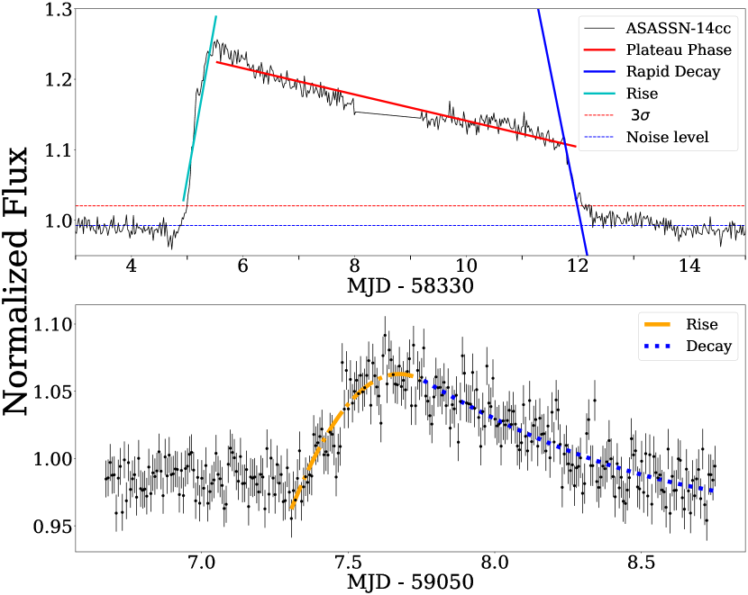
Figure 1: Top Panel: Zoom-in of the superoutburst of ASASSN-14cc in Sector 1 showing how we determine the duration of the SO for our sources. The SO is divided into 3 different phases: the rise (shown in solid cyan), the plateau (shown in solid red line), and the decay (shown in solid blue). The beginning of the SO is defined as the moment in which the flux is $3\sigma$ above the average noise level (dashed red line), the noise level is shown in the dashed blue line. We define the beginning of the SO ’plateau’ as the maximum of the LC and the end of the phase as where the two solid lines meet. Bottom Panel: A further zoom-in on the outburst of ASASSN-14cc in Sector 27 with the fit for the rise and decay overplot to the TESS LC.

4 Results and discussion

In total, 9 sources showed outbursting activity during our campaigns. Given the diverse behaviour of the outbursts in AM CVns, we present the results for each source along with the discussion regarding the possible nature of their variable behaviour.

Table 1: Table of the sources that showed either a superoutburst (SO) or a normal outburst (NO) as seen by TESS. For the orbital period, (p) implies the predicted orbital period based on the outburst properties (Levitan et al., 2015) and (sh) means superhump period, which is typically close to the orbital period and longer by a few percent. Magnitude range taken from Ramsay et al. (2018) and van Roestel et al. (2021).

Source	Period (min)	$\Delta$ mag	TESS Sectors [ISO date]	No. SOs and outbursts	SO duration (day)	Comments
ASASSN-14cc	22.5 (sh)	16 – 20 (V)	1 [2018-07-25 to 2018-08-22] 27-28 [2020-07-05 to 2020-08-25 ]	2 SOs and 3 NOs	7.2	No precursor detected in both SO SO1: 58334.99 to 58342.06 MJD SO2: 59067.46 to 59074.65 MJD
PTF1 J2219+3135	28 (candidate)	16.2–20.6	16 [2019-09-12 to 2019-10-06 ]	1 NO	$-$	Periodicity in normal outburst
V803 Cen	26.6	12.8–17.0	11 [2019-04-23 to 2019-05-20]	at least 4 NOs	$-$	Very activate many fainter outbursts and some possibly confused with the background
PTF1 J0719+4858	26.8	15.8–19.4	20 [2019-12-25 to 2020-01-20]	1 SO, 3 echo outbursts	5.2	Precursor and at variable echo outbursts with increase brightness after the plateau SO: 58852.93 - 58858.12 MJD
KL Dra	25	16.0–19.6	14-26 [2019-07-18 to 2020-07-04]	5 SOs and many echos/normal outbursts	6	TESS LC first reported by Duffy et al. (2021) SO1: 58789.17-58796.19 SO2: 58852.45-58858.50 SO3:58916.74-58922.059
CP Eri	28.4	16.2–20.2	4 [2018-10-19 to 2018-11-14] 31 [2020-10-22 to 2020-11-16]	1 SO and 1 echo O	5.8	Short precursor and at least one echo outburst SO: 58427.97 - 58433.82 MJD
SDSS J1043+5632	28.5 (p)	17.0–20.3	21 [2020-01-21 to 2020-02-18]	1 SO and 8 echo outbursts	6	Precursor and many echo outbursts. SO: 58878.97 - 58885.013 MJD
Gaia 16all	31.1 (candidate)	16.2 – 20.6 (G)	1-13 [2018-07-25 to 2019-07-17] 27-33 [2020-07-05 to 2021-01-13]	3 SOs 1 NO	5.4	Limit on recurrence time and many echo outbursts SO1: 58442.510 - 58447.887 MJD SO2: 58642.011 - 58647.556 MJD SO3: > 3.7 MJD
ZTF18abihypg	$31.2$ (p)	15-19.9	16-17 [2019-09-12 to 2019-11-02] 24 [2020-04-16 to 2020-05-12]	2 NOs	$-$	ZTF LC reported by van Roestel et al. (2021)

4.1 ASASSN-14cc: A system with normal outbursts and superoutbursts with no precursors

ASASSN-14cc was discovered in outburst by ASAS-SN and later confirmed by Kato et al. (2015) as an AM CVn, who also performed follow-up during four superoutbursts and measured the period of the superhumps to be 22.5 min.

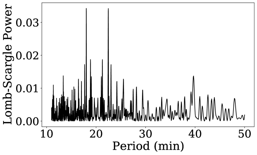
Figure 17: Lomb-Scargle ASASSN-14cc in Sector 27. The periodogram shows the superhump period at 22.5 minutes, and another peak at 18.1 minutes which is the beat period between the superhump period and the TESS sampling of 10 minutes.

ASASSN-14cc was observed by TESS in three sectors (1, 27, 28). Sector 1 was observed from 58324.8 MJD (2018-07-25) to 58352.8 MJD (2018-08-22) with 30-minutes cadence (see Fig.2). Sectors 27 and 28 were observed with a 10-minutes cadence from 59035.8 MJD (2020-07-05) to 59086.6 MJD (2020-08-25, Fig. 2). The final part of Sector 27 shows a normal outburst, while Sector 28 shows a superoutburst. The fast cadence of Sector 28 allowed us to check for periodic variability during the plateau phase of the superoutburst. We find a peak in the periodogram at 22.5 min that agrees with the superhump period for this source found by Kato et al. (2015) (see fig. 17 in the Appendix).

The LCs of ASASSN-14cc (Sector 1 and 28) where SOs where recorded do not show a precursor. The fact that a precursor is not observed in either SO indicates that such behaviour is not due to artefacts, but rather, it is intrinsic to the source. This behaviour is contrary to that seen in SOs of other WD systems studied at short cadence, including some DNe observed with Kepler (Cannizzo et al., 2012) and recently the AM CVn system KL Dra, also observed with TESS (Duffy et al., 2021), where a precursor was detected. However, some SOs in SU UMa-Type DNe have also shown a lack of precursor, which has been revealed using high cadence photometry from Kepler (e.g. Kato & Osaki, 2013).

In a refined version of the TTI model, Osaki & Meyer (2003) explained that the lack or presence of a precursor depends on whether the accretion disk passes the 3:1 resonance radius and reaches the tidal truncation disk or not. According to that model, if the tidal truncation radius is reached, the matter that is damped at that radius causes a gradual decay without a precursor. In this way, SU UMas with large mass ratios can show SOs with and without precursors. Under this model the sizes of the accretion disks would be different for systems with and without a precursor, being larger in the cases where a precursor is not observed. Uemura et al. (2005) proposed that the behaviour of $\dot{P}_{sh}/P_{sh}$, where $P_{sh}$ is the superhump period, is related to the amount of gas around and beyond the 3:1 resonance radius. That ratio is positive for longer time if the amount of mass is larger. The transition from positive to negative $\dot{P}_{sh}/P_{sh}$ would be explained by the depletion of gas.

The lack of a precursor during the superoutburst of ASASSN-14cc suggests that an analogous situation might be occurring. Unfortunately, despite the fact that we have detected superhumps during the superoutburst, we are unable to study their evolution given our current coverage. Higher signal-to-noise and shorter cadence would be needed to test whether the scenario proposed by Uemura et al. (2005) is valid or not in AM CVns.

Using the method described in the data analysis section, we place some limits on the duration of the superoutburst of ASASSN-14cc. In Sector 1, the superoutburst lasted 7.1 days and the ‘plateau’ phase lasted 6.2 days. These numbers were similar for Sector 28 in which the superoutburst and the ‘plateau’ phase lasted 7.2 and 6.2 days, respectively. This conflicts with previously reported values for the duration of the superoutbursts for this source. For example, recently, Duffy et al. (2021) using ground-based data reported a superoutburst duration of $14\pm 2.2$ days. Considering the cadence and coverage of that data set (also reported previously by Kato et al., 2015), and the coverage and cadence of our TESS data, it is possible that the change in the duration of the SO is intrinsic to the source, perhaps due to a change in the size of the accretion disk, or due to changes in the mass transfer rate.

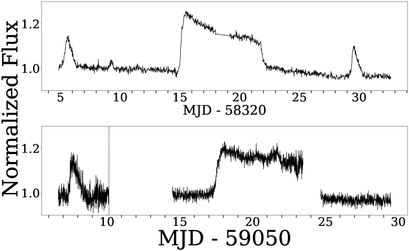
Figure 2: LC from sector 1 at 30-minutes cadence (top panel) and sector 27-28 at 10-minutes (bottom panel) for ASASSN-14cc. The LC in sector 1 (top panel) shows no precursor and a normal outburst before and after the SO. The SO of sectors 28 also lacks a precursor before the SO and an outburst  10 days before the SO. The end of the LC of the SO in sector 28 is contaminated by the background but the end of the ’plateau’ phase and beginning of the fast decay phase is still clear. The dashed black line represents the division between sector 27 and 28.

4.2 PTF1 J2219+3135: an AM CVn with a possible 28 minutes period

PTF1 J2219+3135 was discovered by Levitan et al. (2013). It was observed by TESS in sector 16 from 58738.2 MJD (2019-09-12) to 58762.8 MJD (2019-10-06). This source was observed at 2-minutes cadence and showed an outburst (fig. 3).

The period of this source is not known. Based on the outburst properties, it has been predicted to be 26 minutes (Levitan et al., 2015). With the 2-minute cadence data we search for periodicity during the normal outburst.

The periodogram shows a peak at 27.7 minutes (fig. 4). We also performed PDM analysis and found that the $28.1$ min value minimizes the variance of the LC (inset Fig. 4). This gives a FAP of 0.12 for the period found by PDM. Because the statistical significance for the detection is marginal, further confirmation via spectroscopy is required, but the agreement between the candidate photometric period and the period predicted by the outburst properties is strongly suggestive and should be taken as good motivation to design a search optimized for periods in the 25-30 minute range.

If the period is real, it might represent the orbital period of the source; we cannot, however, discard the possibility that this periodicity is the superhump period since superhumps have been observed during normal outbursts of SU UMa systems (Imada et al., 2012; Kato et al., 2012). If this period is confirmed as the superhump period, this would make PTF1J2219+3135 the first AM CVn showing superhumps during normal outbursts.

Recently Duffy et al. (2021) reported a ground-based LC for this source but the authors stress that the sampling was not optimal. Their data suggest that normal outbursts occur for this source, but the authors mentioned they could not "show convincing evidence of normal outbursts in PTF1 J2219+3135" or measure the duration of these putative normal outbursts. Here we confirm their suspicion and show the LC of an outburst with a duration of roughly  1 day. This adds to the few AM CVns that convincingly show normal outbursts and not only SOs.

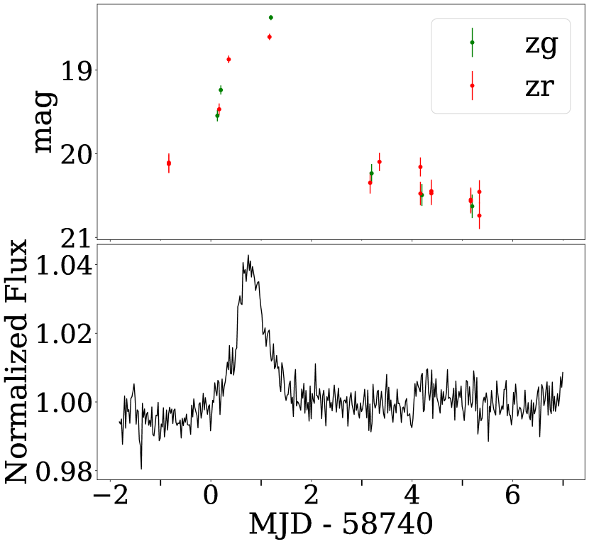
Figure 3: LC for PTF1 J2219+3135 from sector 16 from ZTF (top panel) and TESS (bottom panel). The normal outburst seen with TESS is also seen in ZTF data as $\sim 1.5$ mag outburst. This source was observed at 2-minute cadence

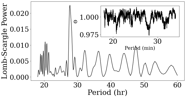
Figure 4: Lomb-Scargle periodogram for the decay part of the outburst of PTF1J2219+3135. The peak corresponds to a period of 27.7 minutes. This period is also recovered using PDM (inset).

4.3 V803 Cen: normal outbursts with variable amplitude

The first high-speed photometry for this object was reported by O’Donoghue et al. (1987), who classified it as an AM CVn and found a periodicity of 26.85 minutes (1611 seconds) for the source, likely a superhump period. A spectroscopic study by Roelofs et al. (2007) later revealed the orbital period to be $1596.2\pm 1.2$ s.

In 2000, Patterson et al. (2000) concluded that V830 had several distinct states: 1) a high state that lasts for 3-12 days with $V=12.7-13.3$, 2) a low state with $V=17$ and duration of at least 10-30 days, and 3) a ‘cycling state’ in which the star varied rapidly between $V=13.4-14.5$ with a period of $22\pm 1$ hr.

Regarding the cycling state, Patterson et al. (2000) concluded that the brightenings in the cycling state followed the Kukarkin-Parenago (Kukarkin et al., 1969; Antipova, 1987) relation for DNe and novae, and concluded that these were ‘normal’ outbursts similar to the ones found in dwarf novae CVs. Contrary, Kato et al. (2001) equated this ‘cycling’ state as similar to the standstills that are observed in Z Camelopardalis (Z Cam) DNe systems, and classified this system (along with CR Boo) as peculiar helium ER UMa-type stars. Later, Kotko et al. (2012) using the Patterson et al. (2000) cycling light curve tried to model these systems and suggested the existence of superoutbursting Z Cam type AM CVns.

This source was monitored in sector 11 by TESS from 2019-04-23 to 2019-05-20 at 30 minutes cadence. We do not observe any superoutbursts, but we do see some outbursts in the LC (Fig. 5). The recurrence time of superoutbursts for this source was found to be $\sim 77$ days by Kato et al. (2004), therefore it is not surprising that we do not detect any in our 27 day monitoring with TESS.

The LC of fig. 5, shows the detailed behaviour of the partially detected "supercycle" for this AM CVn. During quiescence this object has a magnitude close to the TESS detection limit. Thus, we are sensitive to all brightness increases, with errors in their duration of no more than a few hrs. From that figure one can also see that the behaviour of the normal outbursts in V803 Cen is very peculiar. A ‘high amplitude’ outburst is followed by at least one very small amplitude outburst, which also has a shorter duration. One possible explanation is that in the case of the larger outbursts, the heating front reached the outer disk radius and the smaller outbursts are produced when the front does not reach the outer disk regions. This happens when the mass transfer rate is relatively low and the disk mass does not grow enough between two normal outbursts. We note that the relative shapes between the high and short amplitude outbursts resembles somehow to the "stunted outburst" phenomenology seen in some nova-like systems (e.g. Honeycutt1998AJ....115.2527H; Ramsay2016MNRAS.455.2772R). However, we believe it is unlikely that this is more than a coincidence, given that the nova-like systems have significantly higher mean mass transfer rates, and longer orbital periods (and hence larger expected disk-crossing timescales), but further theoretical work should be done to determine more conclusively whether these phenomena might be related.

The behaviour shown by V803 Cen heavily contrasts with the models by Kotko et al. (2012) for Z Cam like AM CVns, where the amplitude of the normal outbursts gradually increases as they are closer to the next SO. Under that model that behaviour is the result of combining mass transfer modulations with the EMT. The TESS LC then argues against such a model for V803 Cen. Instead, it supports more a model that includes the DIM with a larger metallicity and no substantial change of $\alpha$ during the hot and cold states (see e.g. Fig. 5 of Kotko et al., 2012).

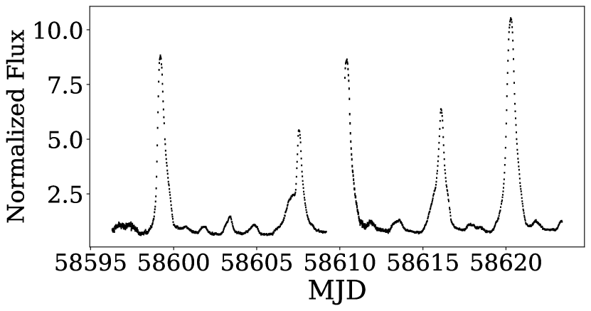
Figure 5: LC of V803 Cen in sector 12 at 30-minutes cadence showing continuous normal outburst of changing amplitudes.

4.4 PTF1 J0719+4858: evidence for enhanced mass transfer

PTF1 J0719+4858 was discovered using data from the Palomar Transient Factory (PTF) by Levitan et al. (2011). The same authors measured an orbital period of $26.77\pm 0.02$ minutes via spectroscopy. Then Han et al. (2021) found a superhump period of 1659.85(13) s (27.66 minutes). Due to its faintness ($g\sim 19$ in quiescent), the outburst behaviour of PTF1 J0719+4858 has not been very well studied. Recently, Duffy et al. (2021) reported on ground-based observations of the source where SOs were detected but they did not report the presence of NOs between SOs.

This AM CVn star was observed in TESS sector 20 from 58842 MJD (2019-12-25) to 58868.3 MJD (2020-01-20). Unlike Duffy et al. (2021), a small amplitude ($r\sim 18.4$ mags) outburst was detected on 58846.24 MJD which is confirmed by the ZTF data as shown in figure 6. Unfortunately, the ZTF data does not allow us to precisely determine the duration of the event due to the lack of coverage, while the TESS data does not constrain the duration due to the faintness of the object, which rapidly felt below the detection limit. However, with the TESS and ZTF data the recurrence time of  10 days for normal outbursts reported for this binary by Levitan et al. (2011) was not observed. Considering that TESS only observed $\sim 10$ days before the start of the SO and some of the reported NOs by Levitan et al. (2011) are close to the detection limits of TESS ($g\sim 18.4$), the recurrence might be hard to confirm without help from other surveys.

In addition to the NO, a SO was also observed. The SO shows a precursor and has a total duration of 5.19 d. Interestingly, after the end of the superoutburst the binary did not reach the original quiescence level. Instead, a series of echo outbursts occurred. They had durations of 0.7, 2 and 5 days, respectively (fig. 6). The amplitude of the echo outbursts was also variable. The whole behaviour observed by TESS was mirrored in the ZTF data. Due to 30-minute sampling for this source (larger than the expected superhump period), a period analysis was not performed.

Kotko et al. (2012), modelled the behaviour of PTF1 J0719+4858 as a helium SU UMa star under a DIM with accretion-irradiation mass transfer rate increase. While the LC obtained by these authors is not totally similar to the one observed by TESS, there are characteristics that are broadly consistent with expectations from the DIM with enhanced mass transfer. First, the presence of a precursor is typical of the EMT model. Second, there is an observed gradual increase in the flux (and hence magnitude) of the echo outbursts, especially evident between the first and the second one. This increase can be explained because during each echo outburst the disk gains more mass than it loses due to accretion. This leads to an accumulation of mass and the surface density of the disk then increases as well. Furthermore, the duration of the echo outbursts increases. The fact that the binary does not reach the original quiescent level after the SO, but instead it stays stuck at a higher flux, indicates changes in the mass transfer rate (see e.g. Hameury & Lasota, 2021). All these characteristics are typical of the EMT model. The observations of PTF1 J0719+4858 then argues for the need to account for EMT mechanisms in the DIM in AM CVns with $P_{orb}$ shorter than 30 min. This is not surprising as such mechanisms have been shown to exist at longer periods (Rivera Sandoval et al., 2020b, a) where enhanced mass transfer and not disk instabilities are the main cause for the outbursts.

4.4.1 The colour evolution of PTF1 J0719+4858

This source was also observed simultaneously with ZTF in two different filters, $g$ and $r$, (fig. 6), allowing us to study the colour evolution of the SO as done in Rivera Sandoval et al. (2020a). Fig. 7 shows the colours selected from the data points fig . 6. The colours of the outbursts are bluer than $g-r=0$, indicative of temperatures well above $10^{4}$ K.

The first point in fig. 7 is due to the very small outburst detected, which did not heat the disk enough to be the dominant component. However, as the SO occurs, the binary becomes bluer and brighter. The next point is redder compared to the plateau phase of the SO because it corresponds to data obtained during the first rebrightening. However, its colour indicates that the disk is still very hot. As the rest of the rebrightenings occur, the system becomes bluer and thus hotter. At the end of the series of rebrigtenings, the binary finally turns redder and fainter because it is going back to its quiescent colour. The behaviour of PTF1 J0719+4858 during SO is very similar to that of the 46 min AM CVn SDSS J141118+481257, but opposite to the one of the longer period AM CVns SDSS 1137 and SDSS 0807 (Rivera Sandoval et al., 2020a), indicating that the triggering mechanism of the SO is very likely not the same that in these two long-period systems.

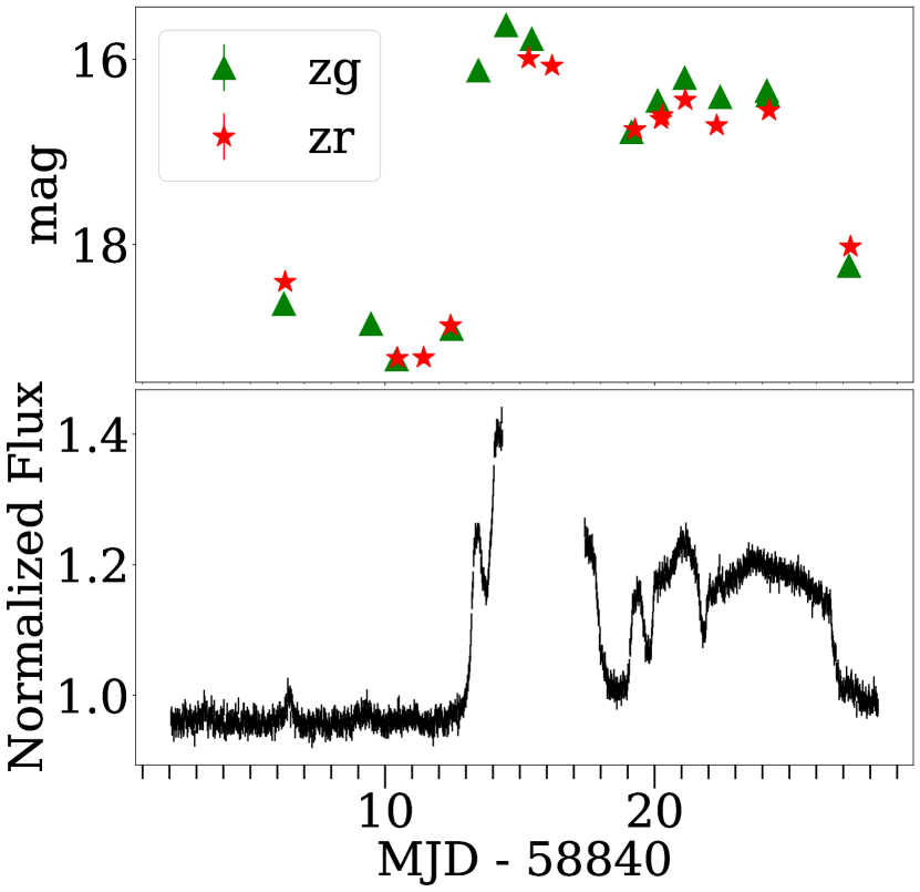
Figure 6: LC from ZTF (top) and TESS (bottom) LC of PTF1 J0719+4858 from sector 20 at 30-minute cadence. The data from the middle of the plateau phase of the SO is contaminated with background and taken out for clarity. The LC shows a small outburst before the SO and at least 3 echo outbursts of increasing duration and variable brightness after the SO.

Figure 7: Evolution of the colour of PTF1 J0719+4858 from the ZTF points shown in fig. 6. For each of the ZTF $r$ magnitudes, we select the closest $g$-band measurement in time, and require that they data points be taken $<$5 hours apart to be plotted. The inverted triangle corresponds to the normal outburst around 58846 MJD before the SO, the filled circles are the data points after the NO and until the end of the SO, and the upright triangles are the colours for the rebrightenings after the SO. The colours corresponds to the difference between the date of when the r value was taken and the maximum of the SO. Negative numbers indicate that data were obtained before the maximum of the SO, and positive numbers refer to dates after the maximum of the SO. The coverage of the SO is not complete but the data show that as the SO develops, the source is bluer and brighter, returning to redder colours at the end of the echo outbursts.

4.5 KL Dra: a frequently outbursting AM CVn shows further evidence for enhanced mass transfer

The object KL Dra was first discovered in outburst as a candidate supernova (Schwartz, 1998). Relatively soon after its discovery, however, it was identified via spectroscopy as a AM CVn system (Jha et al., 1998) and since then, it has been studied extensively in many wavelengths including X-ray and optical. (e.g Wood et al., 2002; Ramsay et al., 2010). It has an orbital period of 25 minutes, superoutburst recurrence time of about 60 days, and the typical superoutburst duration has been reported to be $\sim 15$ days by Ramsay et al. (2010) and more recently to be $10\pm 0.7$ days by Duffy et al. (2021), although we re-visit the issue of the outburst duration here. All sectors for KL Dra were recorded with 30 minutes cadence so we cannot perform searches for superhumps or orbital periodicity.

The TESS LC of this source was first studied by Duffy et al. (2021) where they reported for the first time evidence for precursors in AM CVn systems. KL Dra was continuously observed from sectors 14 to 26 (58682.87-59034.62 MJD). There were two sectors (15, 17) in which we could not resolve the source from the background.

We focused on the SO properties and compare them to other AM CVns also observed by TESS. Fig. 8 shows examples of SOs from KL Dra observed by TESS. Remarkable similarities are observed between these LCs and that of PTF J0719+4858 (Fig. 6), particularly in the shapes of the echo outbursts after the plateau phase of the SO. Similar to PTF J0719+4858, the duration of the echo outbursts seems to be variable, with increasing duration and amplitudes for the later echoes relative to the first echoes (fig. 8). In both systems a precursor is also observed. Given the similarities between KL Dra and PTF J0719+4858, one can apply analogous arguments to explain the behaviour of KL Dra.

We calculate the duration of the SOs. For sector 18 we get a duration of the SO of $\sim 7$ days from 58789.17 to 58796.18 MJD. This is substantially shorter than the value ($\sim 15$ days) reported previously for KL Dra by Ramsay et al. (2010) and closer to the reported value by (Duffy et al., 2021). The sector 18 rebrightenings do, however, prolong the total period of activity by an additional 9.5 days to a total of about $\sim 16$ days including the SO. The outburst in sector 20 (see fig. 8) shows similar properties to that in sector 18 – a 6 day superoutburst, extended to 15 days by rebrightenings – and the full supercycle in sector 22 is only partially covered by TESS, but it shows the main superoutburst to be similar to those in sectors 18 and 22. Most likely, then, the superoutbursts’ durations have been overestimated due to the relatively poor cadence of the ground-based campaigns used to estimate the typical duration, making the echo outbursts to look as if they were part of the main SO. This highlights the need for observatories like TESS that have continuous follow up of these outbursts, and also indicates that high cadence campaigns on the tails of superoutbursts with ground-based networks of telescopes like AAVSO for bright sources, or LCOGT for fainter objects, would be well-motivated.

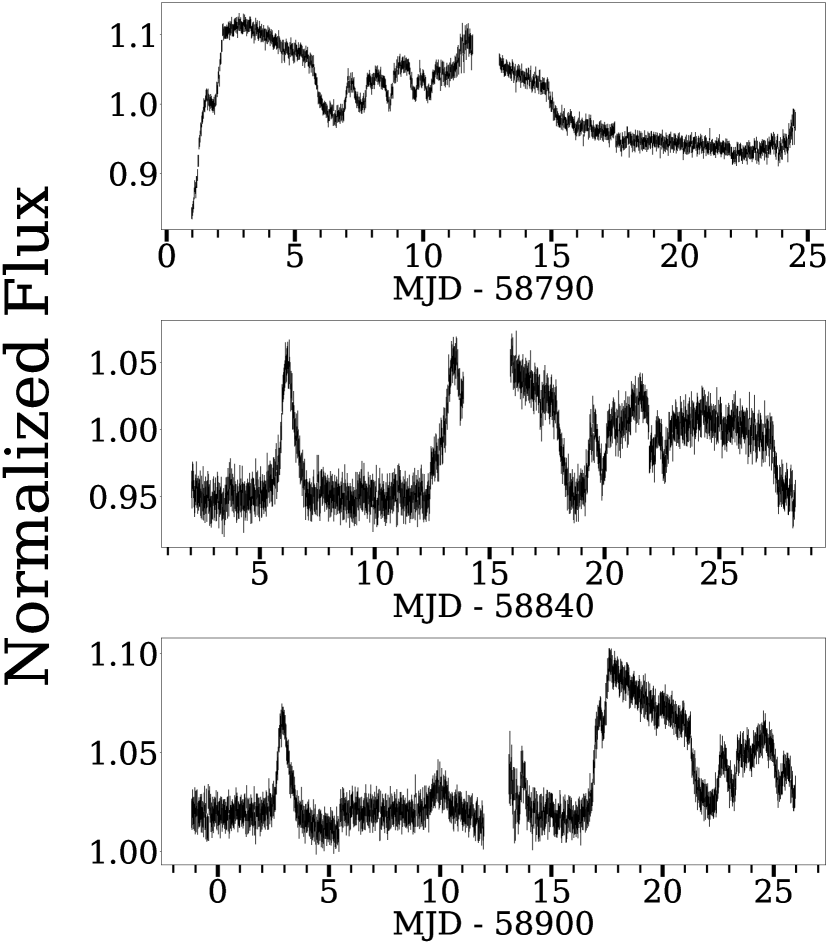
Figure 8: TESS LC of three SO of KL Dra from sector 18 (top panel), 20 (middle panel) and 22 (bottom panel) at 30-minute cadence. All three SOs show similar form with a clear precursor before the SO, and then a series of rebrightenings lasting for $\sim 9$ days of variable length and brightness.

4.6 CP Eri: A short period AM CVn with a short precursor and rebrigthenings

CP Eri is an AM CVn with an orbital period of 28 min (Howell et al., 1991; Abbott et al., 1992). It was in the field of view of TESS in sectors 4 and 31. However, outburst activity was only detected in sector 4, for which the data were acquired with a 30-minute cadence from 58410 MJD (2018-10-19) to 58436 MJD (2018-11-14).

We detected a SO with a precursor in sector 4 (fig. 9) which lasted for 5.8 days. The outburst duration is much shorter than the one previously reported by Levitan et al. (2015), which was $\sim 20$ days. The duration is also much shorter than the one expected from the classical DIM (Cannizzo & Ramsay, 2019). A rebrightening was also detected shortly before the end of the data acquisition, but very likely more rebrightenings occurred which were not recorded. The SO and the rebrightening found with TESS were also detected by ATLAS (Tonry et al., 2018) and ZTF. The characteristics of this source are consistent with the pattern we are finding with the TESS data in which the superoutburst durations seem to be previously overestimated using low-cadence ground-based data because the rebrightenings are merged together with the superoutburst. Due to the sampling frequency, a superhump analysis was not performed.

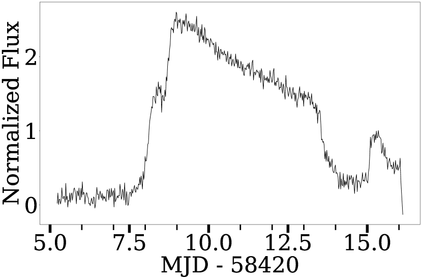
Figure 9: TESS LC from sector 4 for CP Eri at 30-minute cadence. The LC shows a precursor, the SO and at least one echo outburst before the LC ends.

4.7 SDSS J1043+5632: An AM CVn in SO with a series of short-lived echo outbursts

SDSS J1043+5632 was confirmed as an AM CVn via spectroscopy by Carter et al. (2013). Based on the properties of its outbursts in the long-term study carried out by Levitan et al. (2015), an orbital period of 28.5 min was estimated for this source. However, a detailed study of the outbursts of this AM CVn has not been performed until now.

TESS observed this binary in sector 21 from 2020-01-21 to 2020-02-18 at 30-minute cadence. A superoutburst with a precursor, together with a series of 8 echo outbursts were observed. The SO had a duration of 6.04 days, in agreement with the 55-day upper limit determined by Levitan et al. (2015). Unfortunately, the TESS observations did not cover the entire series of echoes, likely leaving unobserved several of them. For the echoes that are visible in fig. 10, we note that they all have very similar (sharp) shapes, amplitudes and short duration (1.1 d). The similarity of that part of the light curve with the recently reported model by Hameury & Lasota (2021) for DNe of the type WZ Sge is remarkable. These authors explained such behaviour by invoking the EMT model. The decay part of the SO is due to a decrease in the mass transfer rate, but in order to reproduce the series of echoes, the mass transfer from the donor needs to be constant for a period of several weeks in DNe (where the echoes occur), which in AM CVns would be of a few days considering the smaller disks. The origin of that behaviour in the mass transfer rate is still unknown, but the fact that after the SO the binary remains above the original quiescent level strongly suggests changes in the mass transfer rate.

It is important to note that in the LC of SDSS J1043+5632 there is no quiescent period between the several echoes. As occurs in the case of WZ Sge (Hameury & Lasota, 2021), that behaviour suggests that the cooling front that propagates from the outer part of the disk towards the inner one is reflected by a heating front, thus making the disk hot. Some of the factors that would influence such behaviour are a hot and small WD (and hence massive) and a lack of truncation in the disk, in order to keep a small inner disk radius (Hameury & Lasota, 2021; Dubus et al., 2001).

4.7.1 The colour evolution of SDSS J1043+5632

This source was also observed simultaneously with ZTF in two different filters, g and r, (fig. 10), allowing us to track the colour evolution of the SO. Fig. 11 shows the colours selected from the data points of fig. 10. The initial colour behaviour of SDSS J1043+5632 is similar to that described by Hameury et al. (2020) for DNe, where the binary initially turns redder and brighter, because despite the fact that the accretion disk is becoming hotter, the contribution of the hot spot is larger. Then, as the SO occurs the system becomes bluer and brighter. After the SO it becomes fainter and redder until the series of echo outbursts starts. The binary then turns again bluer and brighter. We note that the system is, remarkably, bluer than at similar luminosities during superoutbursts, perhaps indicating that the accretion disk spread to larger outer radius during the superoutbursts, and contracted again before the echoes set in. The end of the evolution of the echo outbursts was not depicted in fig. 11 due to the lack of coverage with TESS. As in the case of PTF1 J0719+4858 the behaviour of SDSS J1043+5632 is opposite to the one of the long period systems (SDSS 1137 and SDSS 0807), but more similar to the one of SDSS J141118+481257 (Rivera Sandoval et al., 2020a). This provides further evidence that the colour behaviour is related to the mechanism that triggers the outburst.

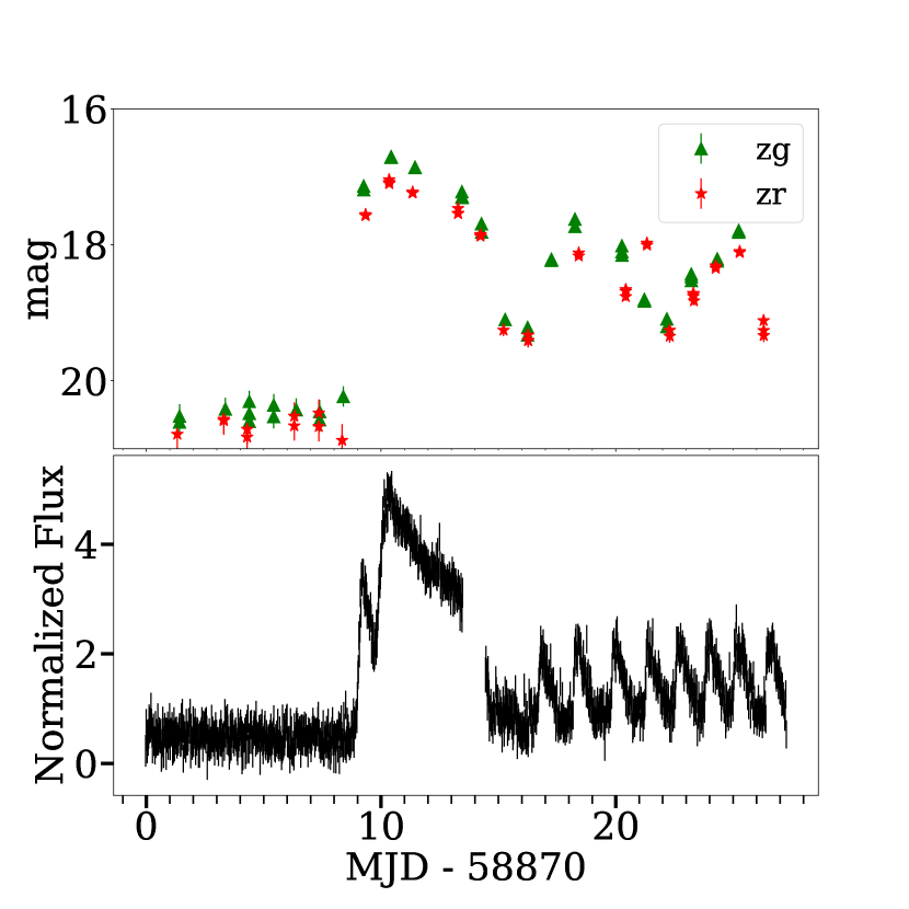
Figure 10: ZTF (top) and TESS (bottom) LC at 30-minute cadence for SDSS J1043+5632 from sector 21. The TESS LC shows the capability of TESS and the month-long continuous coverage of the SO and the rebrigthenings. The TESS LC shows a clear precursor, the SO and a series of short-lived ($\sim 1$ day) echo outbursts lasting for at least 10 days.

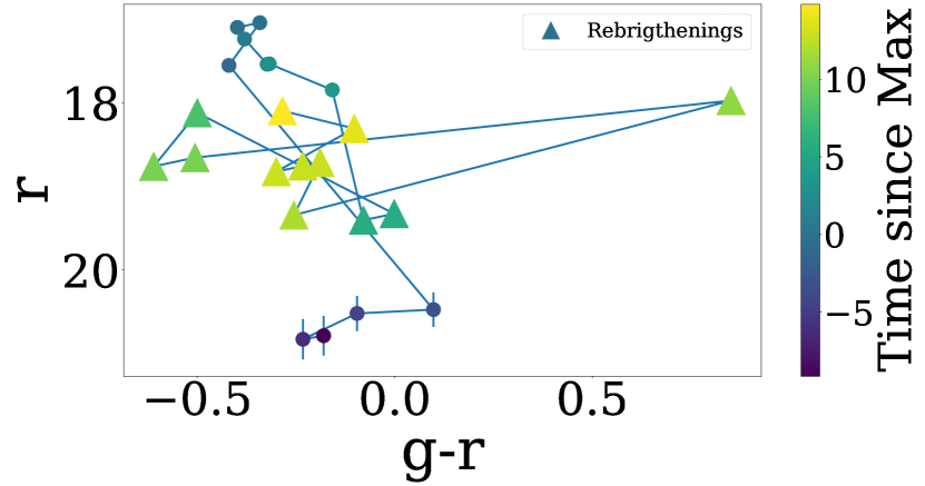
Figure 11: Evolution of the colour of SDSS J1043+5632 from the ZTF points shown in fig. 10. The filled circles are the data points obtained before the SO and until its end. The triangles indicate the rebrightenings after the end of the SO. The colours corresponds to the difference between the date of the when the $r$ value was taken and the maximum of the SO. The colour evolution goes from redder and fainter (before the SO) to bluer and brighter (at the SO). During the rebrigthening phase then the system goes from a period of bluer but fainter to redder and fainter. The right most data point at $r=17.9$ and $g-r=0.8$ is probably not physical and better coverage of colours is needed for this source.

4.8 Gaia 16all: Possible 30-minute period AM CVn with two SOs, normal outburst and dozens of rebrigthenings

This source was discovered in outburst by the Gaia Photometric Science Alerts (Wyrzykowski et al., 2012; Hodgkin et al., 2013) on 2016-04-18 (Delgado et al., 2016). Gaia 16all has two sets of contiguous data. The sectors are contaminated with background stars, the clear periodicity present in the LC is due to a background W UMa. The first set consists of sectors 1 through 13, from 58324.8 MJD (2018-07-25) to 58681.8 (2019-07-17), with a total duration of 357 days. During this period there were two superoutbursts detected, one in sector 5 and another one in sector 12. Their peaks are separated by 203 days, occurring on 58443.8 MJD (2018-11-21) and 58643.3 MJD (2019-06-09), respectively.

The second set is 191 days long, and is composed of sectors 27 to 33. TESS observed this source from 59035.8 MJD (2020-07-05) to 59227.1 MJD (2021-01-13) at 10-minutes and 2-minutes cadence. The gap between sectors 13 and 27 is 354 days long and it is longer than the superoutburst recurrence time observed in the first data set. We see an outburst in sector 28 with a peak at 590674.2 MJD (2020-08-03; fig. 12). This outburst was followed by an SO seen decaying at the beginning of sector 30 with the maximum at 59116.4 MJD (bottom panel of fig. 12).

We use the 2-minute cadence data from sector 30 to search for periodicity. We first detrend the LC of that sector by fitting a polynomial to the SO plateau phase and perform Lomb-Scargle and Phase Dispersion Minimization. From the Lomb-Scargle we get a candidate period of $30.14\pm 0.07$ min and a FAP of 0.017 using the bootstrap method. Using the PDM we get a similar period of $30.12$ min and a FAP of $2.5\times 10^{-13}$ using the method described above in the timing analysis section. The folded LC at the period found with PDM is nonsinusoidal (fig. 14) and this could explain the higher significance found via the PDM method.

We can compare this period to the predicted period based on Gaia 16all outburst recurrence time. Levitan et al. (2015) found the outburst recurrence time and orbital period are related by:

$$y=\alpha P^{\beta}_{orb}+\gamma$$

where $y$ is the outburst recurrence time, $P_{orb}$ is the orbital period in minutes, and $\alpha$, $\beta$, $\gamma$ are fit parameters. Levitan et al. (2015) found the best-fitting values to be $\alpha=1.53\times 10^{-9}$, $\beta=7.35$, and $\gamma$ = 24.7. For a recurrence time of 203 days from the outbursts from sectors 5 and 13, we get a predicted $P_{orb}$ to be 32 minutes, close to the peak of the periodogram found for the source.

Gaia 16all is thus found to be the system with the longest orbital period system with known normal outbursts and superoutbursts. This shows that AM CVn with long recurrence time (in the orders of  200 days) show normal outbursts as well as superoutbursts, suggesting that even at longer periods AM CVns behave like SU Uma as opposed to WZ Sge and show both types of outbursts.

The LC of Gaia 16all resembles the LC of SDSS J1043+5632. Both show a clear precursor before the SO and many echo outbursts after the end of the SO. For Gaia 16all this is visible in all three SOs where each SO is followed by a series of rebrightenings lasting from $\sim 12-15$ days in total and each individual rebrightening with a duration on the order of $\sim 1$ day.

The duration of the three SOs observed with TESS are of 5.4, 5.5 and $>3$ days. These are about $\sim 1$ day shorter than the duration for SDSS J1043+5632 that showed similar pattern. Neither period has been spectroscopically confirmed but SDSS J1043+5632 is predicted to have shorter orbital period and shows longer outburst durations. This contradicts the relation found by Levitan et al. (2015), but given that the periods and durations are relatively similar, it may just be indicative of mild scatter in a relatively robust relation.

Gaia 16all

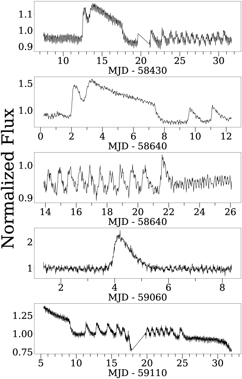
Figure 12: LC for sectors 5, 12, 13, 28 and 30 (top to bottom) from TESS for Gaia 16all at 30-minutes cadence (Panel 1-3 top to bottom) and 2-minutes cadence (last 2 bottom panels). The visible variability in the LC is due to a W UMa variable in the same pixel (21 arcsec) as the AM CVn. The dip on sector 30 (bottom panel) is instrumental and due to the background.

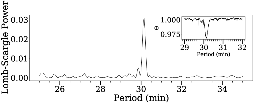
Figure 13: Lomb-Scargle for the 2-minute cadencde LC of Gaia 16all. The periodogram clearly shows an isolated peak at 30.1 minutes. This period is also recovered using PDM (inset).

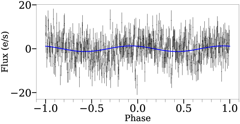
Figure 14: 2-minutes cadence LC folded at 30.12 min for Gaia 16all. We plot only every 10th data point to avoid crowding. The LC is not strictly sinusoidal and could explain the higher significance found using the PDM method. The blue line corresponds to the best-fit sinusoid from the Lomb-Scargle.

4.9 ZTF18abihypg

This source was found as an outbursting source in ZTF by Szkody et al. (2020), and later confirmed via spectroscopy to be an AM CVn by van Roestel et al. (2021), who also looked at the outburts properties using ZTF data. Here we report the observations with TESS. ZTF18abihypg was observed by TESS in 3 sectors (16,17,24) showing two outbursts in sector 16 and sector 24 (fig. 15). Both outbursts show similar profiles and duration of the order of one day. van Roestel et al. (2021) report for this source a high frequency of outbursts, but during the two contiguous sectors of observation by TESS ( 54 days) we only see one outburst, meaning that for this source the recurrence time for normal outburst is larger than 50 days. The cadence of both sectors was of 30-minutes, meaning that we could not perform any periodicity search on the outburst to look for possible superhumps or confirm the orbital period. Based on the SO recurrence time, van Roestel et al. (2021) predicts a period of $\sim 31.2$ minutes, this would imply a long recurrence time for the SO (Levitan et al., 2015), and explains why we did not detect any SO in the two contiguous sectors.

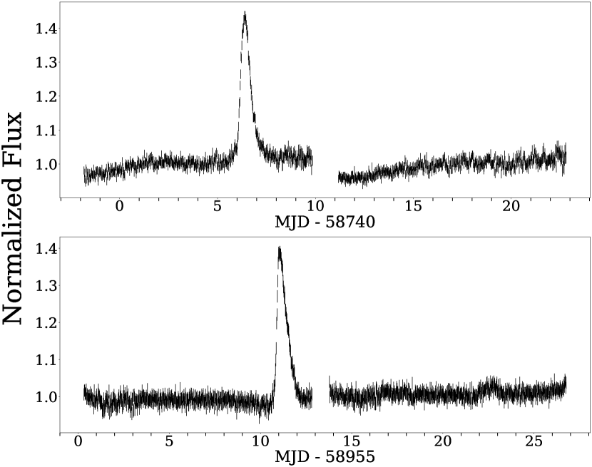
Figure 15: TESS LC for the two outbursts detected by for ZTF18abihypg at 30-minute cadence. The top panel corresponds to sector 16 and the bottom one to sector 24.

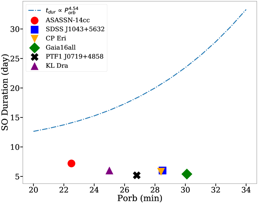
Figure 16: Superoutburst durations vs the orbital period for six sources with SO detected by TESS. The blue dash-dotted line represents the relation found by Levitan et al. (2015). Due to the short time scales of the SO and the echo outbursts, and lack of good coverage as the one provided by TESS, the duration of the SO for many AM CVns might have been overestimated with scarce ground base data. Most likely, then, the superoutbursts’ durations have been overestimated due to the relatively poor cadence of the ground-based campaigns used to estimate the typical duration, making the echo outbursts to look as if they were part of the main SO. Good coverage of the SO of systems with longer orbital period could provide good insight and constraints for models.

4.10 Sources without detected superoutbursts

Other AM CVns were observed by TESS, but no outbursts or superoutbursts were detected. These are shown in Table LABEL:nondetect of the Appendix. Our sample includes several objects at short periods which are known to be persistently in bright states. Most of the systems have long orbital periods, such that even with many sectors observed, an outburst would have low probabilities to be detected considering the long recurrence times. The Levitan et al. (2015) relation between orbital period and superoutburst recurrence time finds that systems with periods longer than about 35 minutes have recurrence times longer than one year. A few of the remaining objects have sufficient number of sectors of data to expect that outbursts would have taken place, but these systems are all sufficiently distant, and had previous outbursts sufficiently faint, that it is expected that they would not be detectable by TESS because they were too faint.

5 Summary

5.1 Precursors

Precursors in SOs of AM CVn were first reported for one system, KL Dra, from TESS data by (Duffy et al., 2021). Here we extend the number of sources that show a clear precursor before the SO to 5. For the 6 systems we observed a SO, ASASSN-14cc was the only system without a clear precursor before the plateau phase of the SO. This might suggest that precursors are a common feature of SOs in AM CVn systems. We also note that the only source without a precursor, ASASSn-14cc, is the system with the shortest orbital period in our sample. We emphasize that this is a small number of sources in the sample and of detected outbursts for each source, so further monitoring of AM CVn systems and their NOs and SOs is needed to verify that in fact precursors are the norm in these types of systems, and to confirm if there is any possible dependence on the orbital period of AM CVns.

5.2 Echo Outbursts

Echo outbursts have been detected before in AM CVns (e.g. Green et al., 2020). Here we used the continuous observations of TESS to study in more detail the echo outbursts of these systems. Of the 6 systems reported here with a SO, 5 of them (PTF1J0719+4858, KL Dra, CP Eri, SDSSJ1043+5632 and Gaia 16all) showed at least one clear rebrightening after the end of the SO. The only system that did not show any echo outburst after its SO detected by TESS was ASASSN-14cc. Like precursors, this could mean that echo outbursts or rebrightening phases are common in SOs of AM CVns. We see echo outbursts for systems of orbital period from 25-32 minutes, but systems with longer orbital period (43,46 minutes) also have shown echo outbursts discovered by other facilities (Green et al., 2020; Rivera Sandoval & Maccarone, 2019), meaning that there is no apparent correlation between the orbital period and the appearance of echo outbursts.

While echo outbursts seem to be a common feature in SO of AM CVns, we find that they show diverse behaviour. For two systems, KL Dra and PTF1J0719+4858, we find a sequence of rebrightenings of varying (and, in fact, increasing) duration from 0.7 days to about   5 days that last for at least 9 days after the end of the SO. Most likely, then, the superoutbursts’ durations in prior work have been overestimated due to the relatively poor cadence of the ground-based campaigns used to estimate the typical durations, merging the echo outbursts with the main SO (Fig.16). As discussed in the main text for both sources, the shape of the echo outbursts for these two systems points towards evidence for enhanced mass transfer in these binaries.

The other three systems (CP Eri, SDSS J1043+5632 and Gaia 16all) that showed echo outbursts showed different characteristics, they are more similar to the ones in the dwarf novae EG Cancri and WZ Sge (Patterson et al., 1998, 2002). They show a series of similar short-lived ($\sim 1$ day) echo outbursts for up to 15 days after the SO. This could be explained due to an increase in the mass transfer rate in the DIM model (Hameury & Lasota, 2021).

We stress again that this is still a small number of observed AM CVns and SOs for each system. Therefore, additional monitoring is necessary to understand the different types of echo outburst in AM CVns and characterize which parameters determine their nature, e.g. orbital periods, whether the donor is a white dwarf or a helium star, chemical composition, long term history of mass transfer and perhaps other parameters might all be important.

5.3 Outbursts Colors

For two sources, SDSS J1043+5632 and PTF1 J0719+4858, we had simultaneous TESS and ZTF data for at least part of the SO. Following the approaches by Rivera Sandoval et al. (2020a), we look at the color evolution of these systems. Both systems showed similar behaviour to SDSS J141118+481257 in that they become bluer as it moves on the rising phase of the outburst, and it is bluest and brightest during the peak. After the SO, the binary becomes redder and fainter reaching colours similar to those before the superoutburst. This behaviour is similar to dwarf novae outbursts and predicted by the DIM (Hameury et al., 2020).

6 Conclusions

The sample size of sources and outbursts is still not sufficient to make broad statistical statements about the outburst properties, but even from this modest sample of continuous light curves, we can establish several new points of phenomenology of the transient AM CVns.

1. It is clear that there is a wide range of phenomenology in the outburst behaviour of AM CVn systems.

2. Precursors seem to be more common than previously believed. Our data shows that given their extremely short duration these are easy to miss with ground-based imaging studies, explaining why the first precursor was only recently detected using TESS. This shows a previously unappreciated similarity to what had been found for normal CVs with Kepler (Osaki & Kato, 2013).

3. Normal outbursts are relatively common in many AM CVns, and have previously been missed because their durations are often less than a full day, meaning that past light curve sampling was insufficient for robustly discovering them.

4. Many systems show large numbers of echo outbursts associated with a single superoutburst, and frequently, the durations and separations of these increase with time which seems to be associated to variations in the mass transfer rate.

5. Superoutburst durations for many systems in the literature have likely been overestimated in poorly sampled light curves (fig. 16), and represent the sum of the superoutburst duration, plus the duration of the time interval over which the echo outbursts were taking place. This issue is more important for empirical tests of outbursts mechanism models than for understanding the detectability of the superoutbursts, but affects both.

6. Candidate periods are found for two systems which previously did not have orbital periods, PTF1 J2219+135, which shows a marginally significant period of about 28 minutes, and Gaia 16all, which shows a much more significant period of 30.1 minutes. In both cases, these periods are similar to what is expected based on outburst recurrence times, but spectroscopic confirmation would be beneficial.

7. The colour evolution of the systems for which there was ZTF simultaneous coverage with TESS shows that the objects become bluer and brighter when they are closer to the maximum of the superoutburst. That colour trend pattern is opposite the one followed by long-period AM CVns in which the triggering outburst mechanism seems to be EMT. This shows that despite the fact that EMT might be present at orbital periods shorter than 30 min, it does not seem to be the dominant triggering process. From that complementary ZTF data, it is clear that further simultaneous multiwavelength observations of AM CVns in outbursts are needed to characterize the mechanisms involved through their colour evolution.

Data Availability

All data used in this document is public and it can be found in the ZTF and TESS webpages.

Appendix

Appendix A Sources without detected superoutbursts

Table 2: The AM CVn in our sample for which no outbursts were detected with TESS. Periods are taken from Ramsay et al. (2018) except below the double line. Periods with ’(sh)’ next to the numbers are those estimated from superhumps, and (p) denotes systems where the period is estimated based on outburst properties. In some cases, the non-detections are unsurprising because the expected recurrence times are less than once per sector, and sometimes considerably less, but in other cases, the non-detections are unsurprising because past outbursts did not reach TESS detection limits. The magnitude ranges are taken from Ramsay et al. (2018) and the ZTF public survey data.

Source RA (J2000) DEC (J2000) TESS sectors $P_{orb}$ (min) Mag. Range (filter) Comments V407 Vul 19:14:26.09 +24:56:44.6 14 9.5 19.9 (V) direct impact accretor ES Cet 02:00:52.2360 -09:24:31.645 30 10.4 16.5–16.8 direct impact accretor AM CVn 12:34:54.6230 +37:37:44.120 22 17.1 14.2 persistent PTF1J1919+4815 19:19:05.1825 +48:15:06.031 14-15 22.5 18.2–21.8 outbursts peak at $\sim 18$ YZ LMi 09:26:38.7243 +36:24:02.463 21 28.3 16.6–19.6 CRTS J0910-2008 09:10:17.4492 -20:08:12.462 8 29.7 (sh) 14.0–20.4 (g) CRTS J0105+1903 01:05:50.0988 +19:03:17.000 17 31.6 16.3-19.6 PTF1J1632+3511 16:32:39.39 +35:11:07.3 24-25 32.7(p) 17.9–23.0 peak at $V\sim 18$ CRTS J0744+3254 07:44:19.7435 +32:54:48.242 20 33(p) 17.4–21.1 V406 Hya 09:05:54.7498 -05:36:08.482 8 33.8 14.5–19.7 PTF1 J0435+0029 04:35:17.73 +00:29:40.7 5, 32 34.3 18.4 (R) – 22.3 (g) peak at $R$=18.4 SDSS J1730+5545 17:30:47.5876 +55:45:18.463 14-26 35.2 18.5 (V) –20.1 peaks at $V=18.5$ NSV 1440 03:55:17.9490 -82:26:11.305 1,12-13, 27-28 37.5 (sh) 12.4(V) – 17.9(G) $V$=12.4 in outburst V744 And 01:29:40.0646 +38:42:10.442 17 37.6 14.5–19.8 SDSSJ1721+2733 17:21:02.4797 +27:33:01.236 25-26 38.1 16.0–20.1 ASASSN-14ei 02:55:33.2826 -47:50:42.318 3-4, 30 43(sh) 11.9–17.6 (B) SDSSJ1525+3600 15:25:09.5669 +36:00:54.683 24 44.3 20.2 SDSSJ1411+4812 14:11:18.3211 +48:12:57.515 16,22-23 46.0 19.4–19.7 GP Com 13:05:42.4008 +18:01:03.765 23 46.6 15.9–16.3 CRTS J0450-0931 04:50:20.0 -09:31:13 5,32 47.3 (sh) 14.8–20.5 SDSS J0902+3819 09:02:21.3623 +38:19:41.841 21 48.3 13.8 (V) – 20.2 (g) Gaia14aae 16:11:33.9745 +63:08:31.886 14-26 49.7 13.6 (V) – 18.7 (g) ASASSN-17fp 18:08:51.10 -73:04:04.2 12-13 51.0 (sh) 15.7–20+ SDSS J1208+3550 12:08:42.0093 +35:50:25.391 22 53.0 18.9–19.4 SDSS J1642+1934 16:42:28.0669 +19:34:10.124 25 54.2 20.3 SDSS J1552+3201 15:52:52.4801 +32:01:51.018 24 56.3 20.2–20.6 SDSS J1137+4054 11 37 32.3218 +40:54:58.496 22 59.6 19.0 V396 Hya 13:12:46.4403 -23:21:32.601 10 65.1 17.6 SDSS J1319+5915 13:19:54.5178 +59:15:14.563 15-16,22 65.6 19.1 CRTS J0844-0128 08:44:13.6 -01:28:07 8 17.4-20.3 PTF1 J0857+0729 08:57:24.27 +07:29:46.7 8 18.6-21.8 ASASSN-14fv 23:29:55.13 +44:56:14.4 16-17 14.6 (V) – 20.5 (B) ASASSN-21br 16:18:10.44 -51:54:15.8 12 38.6 >17.1-13.6 period from Motsoaledi et al. (2021) ASASSN-21au 14:23:52.820 +78:30:13.370 12 58.4 (sh) 20.6-13.4 (g) Average period and g-mag range from (2021RSAU) ZTF J1905+3134 19:05:11.34 +31:34:32.37 14 17.2 20.90 (g) persistent; period from (Burdge et al., 2020) ZTF J2228+4949 22:28:27.07 +49:49:16.44 16-17 28.6 19.2758(G) persistent, $\sim 19$th mag; period from (Burdge et al., 2020) ZTF18acgmwpt 07:01:15.85 +50:23:21.5 20 17.5 -20.50 (g) from ZTF g ZTF18acnnabo 08:20:47.6 68:04:24.0 20, 26 16.5 -19.8 (g) from ZTF ZTF18acujsfl 04:49:30.1 -02:51:53.7 5,32 15.7 -20.3(g) from ZTF ZTF19abzzuin 08:44:19.7 +06:39:50.2 7, 34 18.1 -21.16(g) from ZTF ZTF18aavetqn 19:18:42.0 +44:49:12.3 14,15 14.9 -19.9(g) from ZTF

Appendix B ASASSN-14cc Periodogram

References

- Abbott et al. (1992) Abbott T. M. C., Robinson E. L., Hill G. J., Haswell C. A., 1992, ApJ, 399, 680
- Antipova (1987) Antipova L. I., 1987, Ap&SS, 131, 453
- Astropy Collaboration et al. (2013) Astropy Collaboration et al., 2013, A&A, 558, A33
- Astropy Collaboration et al. (2018) Astropy Collaboration et al., 2018, AJ, 156, 123
- Balbus & Hawley (1991) Balbus S. A., Hawley J. F., 1991, ApJ, 376, 214
- Buat-Ménard & Hameury (2002) Buat-Ménard V., Hameury J. M., 2002, A&A, 386, 891
- Burdge et al. (2020) Burdge K. B., et al., 2020, ApJ, 905, 32
- Cannizzo (1984) Cannizzo J. K., 1984, Nature, 311, 443
- Cannizzo & Nelemans (2015) Cannizzo J. K., Nelemans G., 2015, ApJ, 803, 19
- Cannizzo & Ramsay (2019) Cannizzo J. K., Ramsay G., 2019, AJ, 157, 130
- Cannizzo et al. (1982) Cannizzo J. K., Ghosh P., Wheeler J. C., 1982, ApJ, 260, L83
- Cannizzo et al. (2012) Cannizzo J. K., Smale A. P., Wood M. A., Still M. D., Howell S. B., 2012, ApJ, 747, 117
- Carter et al. (2013) Carter P. J., et al., 2013, MNRAS, 429, 2143
- Cumming (2004) Cumming A., 2004, MNRAS, 354, 1165
- Czesla et al. (2019) Czesla S., Schröter S., Schneider C. P., Huber K. F., Pfeifer F., Andreasen D. T., Zechmeister M., 2019, PyA: Python astronomy-related packages (ascl:1906.010)
- Delgado et al. (2016) Delgado A., Harrison D., Hodgkin S., Leeuwen M. V., Rixon G., Yoldas A., 2016, Transient Name Server Discovery Report, 2016-481, 1
- Dubus et al. (2001) Dubus G., Hameury J. M., Lasota J. P., 2001, A&A, 373, 251
- Duffy et al. (2021) Duffy C., et al., 2021, MNRAS,
- Earl et al. (2021) Earl N., et al., 2021, astropy/specutils: v1.2, doi:10.5281/zenodo.4603801, https://doi.org/10.5281/zenodo.4603801
- El-Khoury & Wickramasinghe (2000) El-Khoury W., Wickramasinghe D., 2000, A&A, 358, 154
- Feinstein et al. (2019) Feinstein A. D., et al., 2019, PASP, 131, 094502
- Fontaine et al. (2011) Fontaine G., et al., 2011, ApJ, 726, 92
- Green et al. (2018) Green M. J., et al., 2018, MNRAS, 477, 5646
- Green et al. (2020) Green M. J., et al., 2020, MNRAS, 496, 1243
- Hameury (2020) Hameury J. M., 2020, Advances in Space Research, 66, 1004
- Hameury & Lasota (2021) Hameury J. M., Lasota J. P., 2021, arXiv e-prints, p. arXiv:2104.02952
- Hameury et al. (2020) Hameury J. M., Knigge C., Lasota J. P., Hambsch F. J., James R., 2020, A&A, 636, A1
- Han et al. (2021) Han Z., Soonthornthum B., Qian S., Sarotsakulchai T., Zhu L., Dong A., Zhi Q., 2021, New Astron., 87, 101604
- Hodgkin et al. (2013) Hodgkin S. T., Wyrzykowski L., Blagorodnova N., Koposov S., 2013, Philosophical Transactions of the Royal Society of London Series A, 371, 20120239
- Horne & Baliunas (1986) Horne J. H., Baliunas S. L., 1986, ApJ, 302, 757
- Howell et al. (1991) Howell S. B., Szkody P., Kreidl T. J., Dobrzycka D., 1991, PASP, 103, 300
- Hunter (2007) Hunter J. D., 2007, Computing in Science & Engineering, 9, 90
- Imada et al. (2012) Imada A., Izumiura H., Kuroda D., Yanagisawa K., Kawai N., Omodaka T., Miyanoshita R., 2012, PASJ, 64, L5
- Jenkins et al. (2016) Jenkins J. M., et al., 2016, in Chiozzi G., Guzman J. C., eds, Society of Photo-Optical Instrumentation Engineers (SPIE) Conference Series Vol. 9913, Software and Cyberinfrastructure for Astronomy IV. p. 99133E, doi:10.1117/12.2233418
- Jha et al. (1998) Jha S., Garnavich P., Challis P., Kirshner R., Berlind P., 1998, IAU Circ., 6983, 1
- Kato & Osaki (2013) Kato T., Osaki Y., 2013, PASJ, 65, 97
- Kato et al. (2000) Kato T., Nogami D., Baba H., Hanson G., Poyner G., 2000, MNRAS, 315, 140
- Kato et al. (2001) Kato T., Stubbings R., Monard B., Pearce A., Nelson P., 2001, Information Bulletin on Variable Stars, 5091, 1
- Kato et al. (2004) Kato T., Stubbings R., Monard B., Butterworth N. D., Bolt G., Richards T., 2004, PASJ, 56, S89
- Kato et al. (2012) Kato T., et al., 2012, PASJ, 64, 21
- Kato et al. (2015) Kato T., Hambsch F.-J., Monard B., 2015, PASJ, 67, L2
- Kotko et al. (2012) Kotko I., Lasota J. P., Dubus G., Hameury J. M., 2012, A&A, 544, A13
- Kukarkin et al. (1969) Kukarkin B. V., et al., 1969, General Catalogue of Variable Stars. Volume_1. Constellations Andromeda - Grus.
- Kupfer et al. (2015) Kupfer T., et al., 2015, MNRAS, 453, 483
- Lasota et al. (1995) Lasota J. P., Hameury J. M., Hure J. M., 1995, A&A, 302, L29
- Lasota et al. (2008) Lasota J. P., Dubus G., Kruk K., 2008, A&A, 486, 523
- Levitan et al. (2011) Levitan D., et al., 2011, ApJ, 739, 68
- Levitan et al. (2013) Levitan D., et al., 2013, MNRAS, 430, 996
- Levitan et al. (2015) Levitan D., Groot P. J., Prince T. A., Kulkarni S. R., Laher R., Ofek E. O., Sesar B., Surace J., 2015, MNRAS, 446, 391
- Lightkurve Collaboration et al. (2018) Lightkurve Collaboration et al., 2018, Lightkurve: Kepler and TESS time series analysis in Python, Astrophysics Source Code Library (ascl:1812.013)
- Linnell Nemec & Nemec (1985) Linnell Nemec A. F., Nemec J. M., 1985, AJ, 90, 2317
- Lomb (1976) Lomb N. R., 1976, Ap&SS, 39, 447
- Masci et al. (2019a) Masci F. J., et al., 2019a, PASP, 131, 018003
- Masci et al. (2019b) Masci F. J., et al., 2019b, PASP, 131, 018003
- Menou et al. (2002) Menou K., Perna R., Hernquist L., 2002, ApJ, 564, L81
- Meyer & Meyer-Hofmeister (1981) Meyer F., Meyer-Hofmeister E., 1981, A&A, 104, L10
- Motsoaledi et al. (2021) Motsoaledi M., et al., 2021, The Astronomer’s Telegram, 14421, 1
- Nelemans et al. (2004) Nelemans G., Yungelson L. R., Portegies Zwart S. F., 2004, MNRAS, 349, 181
- O’Donoghue et al. (1987) O’Donoghue D., Menzies J. W., Hill P. W., 1987, MNRAS, 227, 347
- Osaki (1989) Osaki Y., 1989, PASJ, 41, 1005
- Osaki & Kato (2013) Osaki Y., Kato T., 2013, PASJ, 65, 50
- Osaki & Meyer (2003) Osaki Y., Meyer F., 2003, A&A, 401, 325
- Patterson et al. (1998) Patterson J., et al., 1998, PASP, 110, 1290
- Patterson et al. (2000) Patterson J., Walker S., Kemp J., O’Donoghue D., Bos M., Stubbings R., 2000, PASP, 112, 625
- Patterson et al. (2002) Patterson J., et al., 2002, PASP, 114, 721
- Ramsay et al. (2010) Ramsay G., et al., 2010, MNRAS, 407, 1819
- Ramsay et al. (2018) Ramsay G., et al., 2018, A&A, 620, A141
- Ricker et al. (2014) Ricker G. R., et al., 2014, in Oschmann Jacobus M. J., Clampin M., Fazio G. G., MacEwen H. A., eds, Society of Photo-Optical Instrumentation Engineers (SPIE) Conference Series Vol. 9143, Space Telescopes and Instrumentation 2014: Optical, Infrared, and Millimeter Wave. p. 914320 (arXiv:1406.0151), doi:10.1117/12.2063489
- Rivera Sandoval & Maccarone (2019) Rivera Sandoval L. E., Maccarone T. J., 2019, MNRAS, 483, L6
- Rivera Sandoval et al. (2020a) Rivera Sandoval L. E., Maccarone T. J., Cavecchi Y., Britt C., Zurek D., 2020a, arXiv e-prints, p. arXiv:2012.10356
- Rivera Sandoval et al. (2020b) Rivera Sandoval L. E., Maccarone T. J., Pichardo Marcano M., 2020b, ApJ, 900, L37
- Roelofs et al. (2005) Roelofs G. H. A., Groot P. J., Marsh T. R., Steeghs D., Barros S. C. C., Nelemans G., 2005, MNRAS, 361, 487
- Roelofs et al. (2007) Roelofs G. H. A., Groot P. J., Nelemans G., Marsh T. R., Steeghs D., 2007, MNRAS, 379, 176
- Scargle (1982) Scargle J. D., 1982, ApJ, 263, 835
- Schwartz (1998) Schwartz M., 1998, IAU Circ., 6982, 1
- Schwarzenberg-Czerny (1997) Schwarzenberg-Czerny A., 1997, ApJ, 489, 941
- Schwarzenberg-Czerny (2003) Schwarzenberg-Czerny A., 2003, in Sterken C., ed., Astronomical Society of the Pacific Conference Series Vol. 292, Interplay of Periodic, Cyclic and Stochastic Variability in Selected Areas of the H-R Diagram. p. 383
- Shappee et al. (2014) Shappee B. J., et al., 2014, ApJ, 788, 48
- Smak (1982) Smak J., 1982, Acta Astron., 32, 199
- Smak (1983) Smak J., 1983, Acta Astron., 33, 333
- Smak (1999) Smak J., 1999, Acta Astron., 49, 391
- Smak (2009a) Smak J., 2009a, Acta Astron., 59, 89
- Smak (2009b) Smak J., 2009b, Acta Astron., 59, 103
- Smak (2009c) Smak J., 2009c, Acta Astron., 59, 121
- Smak (2009d) Smak J., 2009d, Acta Astron., 59, 419
- Smith et al. (2012) Smith J. C., et al., 2012, PASP, 124, 1000
- Solheim (2010) Solheim J. E., 2010, PASP, 122, 1133
- Stellingwerf (1978) Stellingwerf R. F., 1978, ApJ, 224, 953
- Sunny Wong et al. (2021) Sunny Wong T. L., van Roestel J., Kupfer T., Bildsten L., 2021, Research Notes of the American Astronomical Society, 5, 3
- Szkody et al. (2020) Szkody P., et al., 2020, AJ, 159, 198
- Tonry et al. (2018) Tonry J. L., et al., 2018, PASP, 130, 064505
- Tsugawa & Osaki (1997) Tsugawa M., Osaki Y., 1997, PASJ, 49, 75
- Uemura et al. (2005) Uemura M., et al., 2005, A&A, 432, 261
- Vanderspek (2019) Vanderspek R., 2019, in AAS/Division for Extreme Solar Systems Abstracts. p. 333.12
- Virtanen et al. (2020) Virtanen P., et al., 2020, Nature Methods, 17, 261
- Warner (1995) Warner B., 1995, Ap&SS, 226, 187
- Wood et al. (2002) Wood M. A., Casey M. J., Garnavich P. M., Haag B., 2002, MNRAS, 334, 87
- Wyrzykowski et al. (2012) Wyrzykowski Ł., Hodgkin S., Blogorodnova N., Koposov S., Burgon R., 2012, in 2nd Gaia Follow-up Network for Solar System Objects. p. 21 (arXiv:1210.5007)
- York et al. (2000) York D. G., et al., 2000, AJ, 120, 1579
- van Roestel et al. (2021) van Roestel J., et al., 2021, arXiv e-prints, p. arXiv:2105.02261