Consistency testing for invariance of the speed of light at different redshifts: the newest results from strong lensing and type Ia supernovae observations

Abstract

The invariance of the speed of light in the distant universe has profound significance for fundamental physics. In this paper, we propose a new model-independent method to test the invariance of the speed of light $c$ at different redshifts by combining the strong gravitational lensing (SGL) systems and the observations of type-Ia supernovae (SNe Ia). All the quantities used to test the deviation of $c$ come from the direct observations, and the absolute magnitudes of SNe Ia need not to be calibrated. Our results show that the speed of light in the distant universe is no obvious deviation from the constant value $c_{0}$ within the uncertainty based on current observations. Moreover, we conclude that the currently compiled SGL and SNe Ia Pantheon samples may achieve much higher precision $\Delta c/c\sim 10^{-2}$ for the deviation of $c$ than all previously considered approaches. The forthcoming data from the Legacy Survey of Space and Time and Wide-Field InfraRed Space Telescope will achieve more stringent testing for deviation of the SOL (at the level of $\Delta c/c\sim 10^{-3}$) by using our model-independent method. Finally, we discuss the potential ways in which our technique might be improved, focusing on the treatment of possible sources of systematic uncertainties.

1 Introduction

In modern cosmology, although the $\Lambda$ plus Cold Dark Matter model ($\Lambda$CDM model) has withstood the test against most of the observational data, there are still some unresolved issues in the framework of such standard cosmological model: the Hubble tension (Freedman, 2017; Valentino, Anchordoqui & Akarsu, 2020), the cosmic curvature problem (Valentino, Melchiorri & Silk, 2019), and the puzzle of accelerating expansion of the Universe (Cao et al., 2011b; Qi et al., 2018). Besides the consideration of possible inconsistencies in different observational methods, alternative solutions or mechanisms have been proposed to overcome these problems. One interesting idea is to assume that the fundamental constants in physics are effective ones, i.e., vary with cosmic time. Particularly, the constancy of the speed of light (SOL), which is measured at very high precision in the local universe ($c_{0}\equiv 2.998\times 10^{5}$ km/s), constitutes one of the most basic and recognized physical postulates. However, one should note that the idea of possible deviation from constant speed of light, originally discussed by Einstein himself (Einstein, 1907), has been quite debated regarding many theoretical issues (Dicke, 1957; Petit, 1988; Moffat, 1993; Magueijo, 2000; Avelino & Martins, 1999; Moffat, 2016). For instance, some authors claimed that the time variation of dimensioned constants such as $c$ are merely human constructs without any operational meaning Duff (2002), while one could face serious conceptual problems if the status of $c$ in physics is changed (Ellis & Uzan, 2005). On the other hand, the varying speed of light (VSL) concepts have also attracted a lot of attention, due to its extensive applications in investigating fundamental physics and testing results from standard cosmology. For instance, Albrecht & Magueijo (1999) showed that VSL provides an alternative theory to the inflationary mechanism, in order to solve the horizon and the flatness problems in the standard big bang model (Barrow, 1999). Such idea was subsequently supported by Moffat (2002), who pointed out that varying dimensional constants over cosmic history can have profound implications for the understanding of the laws of nature, with significant physical consequences directly measured in experiments and observations. In particular, several observational analyses have been performed to study possible variation of $c$ focusing on its ability to explain the scale-invariant spectrum of Gaussian fluctuations in the cosmic microwave background (CMB) data (Magueijo, 2003).

In spite of a very high precision of the measurement of $c$ at present, it should be noted that most of these measurements have been performed at the Earth’s surface (redshift $z=0$). The observational or experimental data of measuring the SOL in the distant universe can be rarely seen. However, with the rapid development of observational technology in modern astronomy, a variety of observational means and an increasing number of observational data make it possible to measure the speed of light in the distant universe with high precision. Quite recently, Salzano, Da̧browski & Lazkoz (2015) proposed a method to derive constraints on the possible variation of $c$ by using Baryon Acoustic Oscillations (BAO). Their work relies on a simple relation between the maximum of angular diameter distance $D_{A}(z_{M})$ and the Hubble parameter function $H(z)$ at the same redshift $z_{M}$, which can be used to assess the SOL, i.e., $c(z_{M})=D_{A}(z_{M})\cdot H(z_{M})$ at a higher redshift in a simple way. More recently, Cao et al. (2017a) performed the measurement of $c$ at the maximum redshift ($z_{M}=1.70$) using (instead of BAO data) the angular diameter distances from intermediate-luminosity radio quasars calibrated as standard rulers (the maximum redshift is covered by such observational data set). Such methodology was subsequently extended by Salzano (2017) focusing on multiple measurements of $c$ at different redshifts, in which the the degeneracy between the curvature of the universe and the speed of light was also discussed. Moreover, Cai et al. (2016) developed a new model-independent method to probe the constancy of $c$ with the elimination of degeneracy between the SOL and the cosmic curvature. The advantage of their work also lies in the successful reconstruction of $c$-evolution with redshifts, in a fully comprehensive way based on Gaussian Processes (GP) (Seikel, Clarkson & Smith, 2012). However, in their approach one needs the first and second derivatives of luminosity distances, which cannot be observed directly but evaluated numerically. Some other observational tests for varying speed of light in cosmology have also been investigated in the literature (Qi et al., 2014; Salzano, Da̧browski & Lazkoz, 2016; Wang et al., 2019).

Fortunately, one new idea for the extragalactic measurement of $c$ dodging some drawbacks of the previous works has been presented by Cao et al. (2020). The idea is to measure $c$ at multiple different redshift points by the combination of strong gravitational lensing systems (SGL) and observations of ultra-compact structure in radio quasars and its performance has been illustrated on simulated data from the Large Synoptic Survey Telescope (LSST) of Vera Rubin Observatory and the very-long-baseline interferometry (VLBI) data on radio-quasars. Their results showed that the precision of $\Delta c/c=10^{-4}$ level can be achieved at high redshifts. Inspired by the above work, we will combine the currently available SGL data and recent SNe Ia Pantheon sample to perform the measurement of $c$ (Riess et al., 1998; Perlmutter et al., 1999). Although, compared with radio quasars, the redshift range of Pantheon is inferior to radio quasars, the greatest advantage of SNe Ia lies in the large sample available. Therefore, in our work, we use the large sample of real data (SGL and Pantheon samples) to test the deviation of the SOL over a wide range of redshift instead of the maximum-condition redshift $z_{M}$ point. The outline of this paper is as follows. In Section 2 we present the methodology and the data we use. The results and analyses are given in Section 3. Finally, we summarize our main conclusions in Section 4.

2 Methodology and data

2.1 Strong gravitational lensing system

According to the Einstein’s theory of general relativity, the light will change its route in the gravitational field of massive objects. When the background light source (at redshift $z_{s}$), the intervening galaxy acting as lens (at redshift $z_{l}$), and the observer are perfectly aligned or very slightly misaligned, the source is imaged as the so-called Einstein ring. The size of the Einstein ring of the source is related to source-lens distance ratios and the mass distribution model within the lens (Rusin & Kochanek, 2005; Koopmans et al., 2006, 2009). However, it depends on the assumption that the SOL is constant. On the contrary, for a given SGL system, if the source/lens distance ratios (for details see below), the Einstein radius and the mass distribution model are known, one can perform the measurement of a deviation of the SOL from the value $c$ measured in the laboratory.

In general, early-type galaxies act as lenses in the majority of SGL systems detected. Even though their formation and evolution are still not fully understood in details, a singular isothermal sphere model (SIS) can reasonably characterize the mass distribution of massive elliptical galaxies within the effective radius (Ofek et al., 2003; Cao et al., 2016a; Liu et al., 2020). Under this model, the Einstein radius can be expressed as

$$\theta_{E}=4\pi\frac{\sigma_{0}^{2}}{c_{zs}^{2}}\frac{D^{A}_{ls}}{D^{A}_{s}},$$ (1)

where $\sigma_{0}$ is central velocity dispersion of the lens, ${D^{A}_{s}}=D^{A}(0,z_{s})$ and ${D^{A}_{ls}}=D^{A}(z_{l},z_{s})$ denote the angular-diameter distances to the source and between the source and the lens, respectively. Let us introduce the notation concerning the speed of light, which will be used in this paper. In the equation above, $c_{zs}$ is the speed of light $c$ enriched by the subscript to highlight that this is the quantity to be measured from the lensing system extending to the source redshift $z_{s}$. In order to highlight the speed of light whose value we know from laboratory measurements we will use the notation $c_{0}\equiv c$. It is worth noting that the measurement of $c_{zs}$ from strong lensing observations, is derived from geometrical distances related to space-time metric. Such definition of speed of light which enters the Hilbert Einstein action in the standard General Relativity context, is well consistent with that implemented in the previous works (Salzano, Da̧browski & Lazkoz, 2015; Cai et al., 2016). Following recent analysis of the lens mass distribution models (Treu et al., 2006; Cao et al., 2012; Ma et al., 2019; Liu et al., 2019), a more general, spherically symmetric power-law mass distribution $\rho\sim r^{-\gamma}$, where $\rho$ is the total (i.e. luminous plus dark-matter) mass distribution and $r$ is the spherical radius from the center of the lensing galaxy has been widely considered in studies of SGL systems. Assuming that the velocity anisotropy can be ignored and solving the spherical Jeans equations (Koopmans et al., 2006), one can rescale the dynamical mass inside the aperture $\theta_{ap}$ projected to the lens plane to the Einstein radius, and compare it with the mass inside the Einstein radius $\theta_{E}$ obtained from strong lensing data. As a result one gets the following expression:

$$\theta_{E}=4\pi\frac{\sigma_{ap}^{2}}{c_{zs}^{2}}\frac{D^{A}_{ls}}{D^{A}_{s}}\left(\frac{\theta_{E}}{\theta_{ap}}\right)^{2-\gamma}f(\gamma),$$ (2)

where $f(\gamma)$ is a certain function of the radial mass profile slope (Cao et al., 2015, 2020), $\sigma_{ap}$ represents the luminosity averaged line-of-sight velocity dispersion of the lens inside the aperture radius, and $c_{zs}$ is the speed of light to be determined from SGL system. This specific symbol $c_{zs}$ emphasizes the extragalactic measurement of $c$. For a specific SGL system observed in some survey, one can get the Einstein radius $\theta_{E}$, velocity dispersion of the lens inside the aperture radius $\sigma_{ap}$, the redshift of lens and source $z_{l}$ and $z_{s}$. Then, in order to test the deviation of the SOL, it is necessary to obtain the source-lens distance ratio $D^{A}_{ls}/{D^{A}_{s}}$, which is difficult. Let us note that in many previous works, the assumption that the SOL is a fundamental constant of known value, the same reasoning was used to determine $D^{A}_{ls}/{D^{A}_{s}}$ from SGL systems. However, if one assumes the Friedman-Robertson-Walker (FRW) background metric one can use the so-called distance sum rule, i.e., $D_{ls}=D_{s}\sqrt{1+\Omega_{k}D_{l}^{2}}-D_{l}\sqrt{1+\Omega_{k}D_{s}^{2}}$ (Bernstein, 2006; Clarkson, Bassett & Lu, 2008; Räsänen, et al., 2015), where $D$ is the proper distance related to the angular diameter distance as $D(z_{1},z_{2})=D_{A}(z_{1},z_{2})(1+z_{2})$. Hence, one is able express the source-lens (angular diameter) distance ratio in terms of angular diameter distances from lens to observer ($D^{A}_{l}$) and from source to observer ($D^{A}_{s}$)

$$\frac{D^{A}_{ls}}{D^{A}_{s}} = \sqrt{1+[(1+z_{l})D^{A}_{l}]^{2}\Omega_{k}}$$ (3)

$$- \frac{1+z_{l}}{1+z_{s}}\frac{D^{A}_{l}}{D^{A}_{s}}\sqrt{1+[(1+z_{s})D^{A}_{s}]^{2}\Omega_{k}}.$$

One has to keep in mind that our strategy of measuring SOL at different redshifts is still highly-degenerated with cosmic curvature, i.e., there might be a possibility that an incorrect choice of $\Omega_{k}$ could potentially bias the (otherwise) model-independent test of the invariance of speed of light. However, considering the stringent constraints on the spatial curvature $\Omega_{k}=0.001\pm 0.002$ yielded by the recent Plank CMB observations together with the BAO data (Planck Collaboration, 2018), it is reasonable to assume the flat Universe. It is beyond the scope of the present paper to thoroughly discuss the issue of $\Omega_{k}$ with the data we use. In the framework of a flat universe, Eq. (3) could be rewritten as

$$\frac{D^{A}_{ls}}{D^{A}_{s}}=1-\frac{1+z_{l}}{1+z_{s}}\frac{D^{A}_{l}}{D^{A}_{s}}.$$ (4)

Now the SOL measurement from a specific gravitational lensing system is obtained as

$$c_{zs}=\sigma_{ap}\sqrt{\frac{4\pi}{\theta_{E}}\left(1-\frac{1+z_{l}}{1+z_{s}}\frac{D^{A}_{l}}{D^{A}_{s}}\right)\left(\frac{\theta_{E}}{\theta_{ap}}\right)^{2-\gamma}f(\gamma)}.$$ (5)

In addition to this, another issue which needs clarification is the central velocity dispersion of the lens, i.e., whether the measurement of $\sigma_{ap}$ is dependent on the value of SOL. Such issue was extensively discussed by van Dokkum & Stanford (2003), in which they used the near ultraviolet lines blue-ward of the CaII, H and K lines for measuring velocity dispersion, and determined the central velocity dispersions from a fit to a convolved template star spectrum in real space. However, the usual procedure to determine velocity dispersions is to compare a galaxy spectrum with a star spectrum taken through the same spectrograph with the same setup (Rix & White, 1992). Hence, the spectral lines become wider because of the Doppler effect and $\sigma_{ap}$ can be roughly inferred from the observed quantity $c_{0}\Delta\lambda/\lambda$. It should be noted that only dimensionless quantities can have invariant, fundamental meaning, from the perspective of theoretical physics. Therefore, in this analysis we introduce the quantity of $T_{zs}=c_{zs}/c_{0}$, with the following expression of

$$T_{zs}=\frac{\sigma_{ap}}{c_{0}}\sqrt{\frac{4\pi}{\theta_{E}}\left(1-\frac{1+z_{l}}{1+z_{s}}\frac{D^{A}_{l}}{D^{A}_{s}}\right)\left(\frac{\theta_{E}}{\theta_{ap}}\right)^{2-\gamma}f(\gamma)},$$ (6)

Here $T_{zs}$ quantifies the deviation of $c_{zs}$ from $c_{0}$, with $T_{zs}=1$ denoting the invariance of speed of light at different redshifts.

Now one still needs to determine the angular-diameter distances $D^{A}_{l}$ and$D^{A}_{s}$ to the lens and to the source. For this purpose, one could turn to other model-independent astronomical probes, such as SNe Ia (standard candles), gravitational wave signals (standard sirens) or compact intermediate-luminosity radio quasars (standard rulers) to derive the above mentioned distances only according to the redshifts. In this work, we will use the current newly-compiled SNe Ia data (Pantheon sample).

2.2 Strong gravitational lensing sample

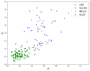
Figure 1: The scatter plot of 161 SGL systems from SLACS, BELLS, SL2S, LSD surveys.

Following the work of Cao et al. (2015), we note that the lens galaxies should ensure the validity of the spherically symmetric hypothesis, which is guaranteed by the following two selection rules: (i) the lens galaxies should be of early-type; (ii) the lens galaxies should not have obvious substructures or close massive companions (not only physical ones but also projected). Recently, Chen et al. (2019) compiled a sample including 161 galaxy-scale strong lensing systems which satisfy the requirements mentioned above. This is currently the largest sample with both high resolution imaging and stellar dynamical data. The data of this sample came from four surveys, 95 systems from the Sloan Lenses Advanced Camera for Surveys (SLACS) (Bolton et al., 2008; Auger et al., 2009, 2010), 38 systems come from an extension of the SLACS survey known as “SLACS for the Masses” (Shu et al., 2015, 2017), 26 systems from the Strong Lensing Legacy Survey (SL2S) (Ruff et al., 2011; Sonnenfeld et al., 2013a, b, 2015), 35 from the BOSS emission line lens survey (BELLS) (Brownstein et al., 2015), 14 systems come from the BELLS (GALLERY) GALaxy-Ly$\alpha$ EmitteR sYstems (Shu et al., 2016a, b), and 5 systems from Lens Structure and Dynamics (LSD) survey (Koopmans & Treu, 2002, 2003; Treu & Koopmans, 2002, 2004), in which the complete information (lens redshift $z_{l}$, source redshift $z_{s}$, Einstein radius $\theta_{E}$ and velocity dispersion $\sigma_{ap}$) can be found in Table. A1 of Chen et al. (2019). The lens and source redshifts cover the range of $0.0625<z_{l}<1.004$ and $0.197<z_{s}<3.595$. The redshift distribution of the lenses and the sources is shown in Fig. 1, where we can see that most SGL systems located at low redshift range come from SLACS.

2.3 Type Ia supernovae observation and Pantheon dataset

In order to get ${D^{A}_{l}}$ and ${D^{A}_{s}}$, we focus on SNe Ia referred to as standard candles of cosmology. The recent SNe Ia sample called Pantheon has been released by the Pan-STARRS1 (PS1) Medium Deep Survey, and contains 1048 SNe Ia covering redshift range from 0.01 to 2.3 (Scolnic et al., 2018). One of the obvious advantages for using this sample is the richness of the sample, and its depth in redshift which means that it extends to higher redshifts than previous data sets such as Union2.1 or JLA (Betoule et al., 2014). The Pantheon catalogue combines the subset of 279 PS1 SNe Ia (Rest et al., 2014; Scolnic et al., 2014) with useful samples of SNe Ia from SDSS, SNLS, various low redshift and HST samples (Scolnic et al., 2018). In general, the use of type Ia SNe, whose lightcurve is characterized by three or four nuisance parameters, involves their optimization along with the unknown parameters of the cosmological model.

Fortunately, a new approach called BEAMS with Bias Corrections (BBC) was applied to the Pantheon data set (Kessler & Scolnic, 2017). With the BBC method, Scolnic et al. (2018) reported the corrected apparent magnitude $m_{B,corr}=m_{B}+\alpha^{*}\cdot X_{1}-\beta\cdot\mathcal{C}+\Delta M$ for all the SNe Ia. Therefore, the observed distance modulus of SNe Ia is simply reduced to $\mu_{SN}=m_{B,corr}-M_{B}$. The scatter plot of 1048 SNe Ia of apparent B-band magnitude and $1\sigma$ uncertainty from Pantheon data set is illustrated in Fig. 2. The total uncertainty of the distance modulus in the Pantheon data set is reduced to the observational uncertainty of the corrected apparent magnitude. For more details one may refer to Scolnic et al. (2018). The luminosity distance of SNe Ia in Mpc is given by a well-known equation of the following form

$$D_{L,SN}=10^{0.2\mu_{SN}+1}.$$ (7)

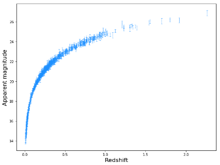
Figure 2: The scatter plot of 1048 SNe Ia apparent magnitude and 1$\sigma$ uncertainty from Pantheon dataset.

Although the SNe Ia do not provide the angular diameter distance directly, a fundamental relation called “distance duality relation” (DDR) could help us get such distance information (Etherington, 1933, 2007; Cao & Liang, 2011; Cao et al., 2016b). More precisely, the luminosity distance and the angular diameter distance at the same redshift $z$ are connected to each other according to $D_{A}(z)=D_{L}(z)(1+z)^{-2}$. Under the assumption of DDR, the combination of Eqs. (6)-(7) will provide the SOL ratio as

$$T_{zs}=\frac{\sigma_{ap}}{c_{0}}\sqrt{\frac{4\pi}{\theta_{E}}\left(1-\frac{1+z_{s}}{1+z_{l}}10^{0.2\Delta m_{B,corr}}\right)f(\gamma)\left(\frac{\theta_{E}}{\theta_{ap}}\right)^{2-\gamma}},$$ (8)

where $\Delta m_{B,corr}=m_{B,corr}(z_{l})-m_{B,corr}(z_{s})$ is the corrected apparent magnitude difference between the redshifts of lenses and sources. It should be noted that the nuisance parameter $M_{B}$ is eliminated, which is beneficial in alleviating the systematics caused by diverse determinations of the absolute magnitude of this standard candle. One may argue that DDR can be violated under certain conditions, e.g., the photons emitted by sources could be affected by various astrophysical mechanisms in the process of propagation, such as dust extinction or more exotic ones like axion conversion (Bassett & Kunz, 2004; Corasaniti, 2006). However, our analysis is not affetced much by this. More specifically, the DDR parameter $\eta=D_{L}/D_{A}(1+z)^{-2}$, which appears when the angular-diameter distance ratio $D_{l}^{A}/D_{s}^{A}$ is related to the luminosity-distance ratio (from SN Ia) gets cancelled, hence it does not introduce any significant uncertainty to the final results. There might still be the issue of redshift dependence of $\eta$ parameter (i.e. cancellation will not be perfect). However, we do not have any strong evidence for this from other DDR studies in the literature.

3 Simulation and Results

In order to implement the methodology described above, for each SGL system with lens redshift $z_{l}$ and source redshift $z_{s}$ known, the corrected apparent magnitude $m_{B,corr}(z_{l})$ and $m_{B,corr}(z_{s})$ should be derived at the same redshift from SNe Ia observations. In order to avoid systematic errors brought by redshift difference between SGL and SNe Ia, a cosmological model-independent criterion should be considered: $|z_{SGL}-z_{SN}|<0.005$, where $z_{SGL}$ represents both redshifts of the lens and of the source.

After the redshift selection criterion we obtained the final sample containing in total 98 systems: 84 systems come from SLACS, 9 come from BELLS and 5 come from SL2S. Following the studies of lensing caused by early-type galaxies (Koopmans et al., 2009; Treu et al., 2006; Cao et al., 2012), the spherically symmetric mass distribution ($\gamma=2.01\pm 0.03$) was applied for the lens model, which was obtained from a joint gravitational lensing and stellar dynamical analysis of a sample of massive early-type galaxies (Koopmans et al., 2006). The individual measurements of deviation of the SOL based on current observations of strong-lensing systems and SNe Ia covering redshift range from $z_{s}=0.197$ to $z_{s}=2.34$ are shown in Fig. 3. Uncertainties have been assessed from the standard uncertainty propagation formula, based on (uncorrelated) uncertainties of observable quantities entering the Eq. (8). The uncertainty of $\gamma$ was also propagated to the total uncertainty budget.

To better describe our results, first, we firstly turn to inverse variance weighting (Bevington et al., 1993) to evaluate the deviation of the SOL, which is often used in meta-analysis to integrate the results of independent measurements, and our assessment is $T_{zs}=0.983\pm 0.013$ (corresponding to $c(z_{s})=2.950(\pm 0.04)\times 10^{5}$ km/s) with full sample. Meanwhile, we have also used a robust non-parametric statistic (Feigelson & Babu, 2012) of calculating the median $Med({T}_{zs})$ and the corresponding median absolute deviation $MAD({T}_{zs})$. The result is $Med({T}_{zs})=0.980\pm 0.131$ (corresponding to median of the SOL $Med({c}({z_{s}}))=2.94(\pm 0.393)\times 10^{5}$ km/s) for full sample. Such approach has been extensively applied to quantify the consistency between the cosmological constant and evolving dark energy in the so-called Om$(z)$ diagnostic (Zheng et al., 2016, 2018). Our findings are in perfect agreement with the results of previous works (Cai et al., 2016; Salzano, Da̧browski & Lazkoz, 2015; Cao et al., 2017a). The SOL derived from the current data on extragalactic sources is consistent with the value $c_{0}\equiv 2.998\times 10^{5}$ km/s within the uncertainty. There is no obvious evidence to support a deviation in the SOL at distant Universe, this is the unambiguous conclusion of our work. Let us compare this result with the work of Cao et al. (2020), where they combined the SGL systems and compact radio sources quasars to constrain $c$, and obtained the speed of light value $c(z_{s})=3.005(\pm 0.06)\times 10^{5}$ km/s. Our results show that currently compiled SGL systems combined with the SNe Ia Pantheon sample may achieve constraints with a higher precision of $\Delta T_{zs}\sim 10^{-2}$ (corresponding to $\Delta c/c\sim 10^{-2}$). The order of magnitude is the same with the previous work of Cao et al. (2020), but the precision for the SOL measurement has doubled by using our method.

Table 1: The deviation $T_{zs}$ and weighted averages of $c$ with corresponding uncertainties from the full sample and three sub-samples.

Sample	Deviation $T_{zs}$	Weighted averages $c\times 10^{5}km/s$
Full	$0.983\pm 0.013$	$2.950\pm 0.04$
SLACS	$0.982\pm 0.017$	$2.945\pm 0.05$
BELLS	$0.904\pm 0.097$	$2.712\pm 0.29$
SL2S	$1.018\pm 0.143$	$3.053\pm 0.43$

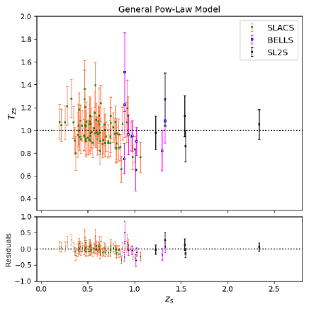
Figure 3: The scatter plot of the deviation $T_{zs}$ of the speed of light and residuals, based on the current SNe Ia observations and strong-lensing systems with power-law lens model.

On the other hand, a lower central value of the deviation of SOL has been obtained, i.e., $T_{zs}=0.983<1$. To explore the reason of this result, we estimated the deviation of the SOL by using SLACS, BELLS and SL2S surveys sub-samples respectively and summarized them in Table. 1. One can note that the deviation measurement of the SOL calculated from SLACS and full sample are almost the same, but the deviation measurement of the SOL evaluated from SL2S with larger uncertainty is higher than from full sample. We can, therefore, infer that the weight of the deviation of SOL assessed from SLACS is greater than the weight of SL2S, and this will leads to a low the deviation of SOL. The leverage of SLACS and BELLS systems is noticeable in Fig. 3, which also illustrates the residual plot for different lens sub-samples. For SL2S sub-sample, their deviation $T_{zs}=1.018>1$ can be a result of their systematics and incomplete samples. Namely, spectroscopic surveys are biased toward smaller Einstein radii. According to Eq. (6), one can infer that the smaller Einstein radius and larger velocity dispersion will yield to larger value for the speed of light, and thus $T_{zs}$ will be greater than one. Therefore, we took a look at the five SL2S strong lensing systems (J020524-93023, J022610-042011, J084847-035103, J084909-041226, and J222148+011542). Their Einstein radii have smaller values (0”.76, 1”.19, 0”.85, 1”.10, and 1”.40 with the mean value 1”.06) than Einstein radii from SLACS survey. This is reasonable, as the source redshift from SL2S is higher than in SLACS, which means the sources from SL2S is farther away, which leads to a smaller Einstein radius. It is good to compare this with the Einstein radius from the whole SL2S sample, because the redshift matching may cause selection bias. The mean value of the Einstein radius from 26 SL2S systems yields 1”.32. Similarly, the mean value of the velocity dispersion of selected five SL2S systems is 255.6 km/s, which is larger than the mean value of 238.9 km/s for the 26 SL2S systems, and further contributes to deviation $T_{zs}>1$. Thus, we may expect that the insufficient sample size will cause some deviations in the SOL.

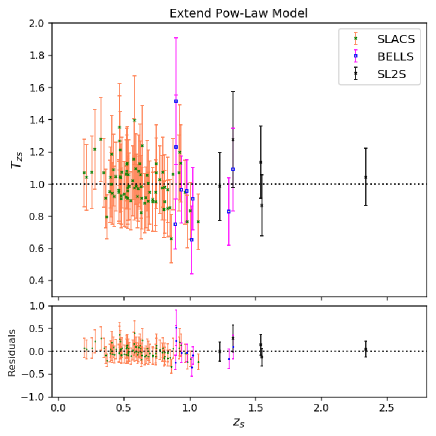
Figure 4: The scatter plot of the deviation $T_{zs}$ of the speed of light and residuals, based on the current SNe Ia observations and strong-lensing systems with extended power-law (EPL) lens model.

There are still several sources of systematics we do not consider in this paper. For instance, whether the use of a different mass distribution models for these lenses could significantly affect the final result. Therefore, we performed a sensitivity analysis and repeated the above calculation using the extend power-law (EPL) lens model, in which the luminosity density profile ($v(r)\sim r^{-\delta}$) is different from the total mass (luminous plus dark matter) density profile $\rho(r)\sim r^{-\alpha}$. Such lens model has found widespread astrophysical applications in the literature (Cao et al., 2016a; Xia et al., 2017; Qi et al., 2019), considering the anisotropic distribution of stellar velocity dispersion $\beta$ (Koopmans, 2005; Chen et al., 2019; Cao et al., 2017b). With the EPL lens parameters $(\alpha,\beta,\delta)$ modeled by Gaussian distributions $\alpha=2.00\pm 0.08$, $\delta=2.40\pm 0.11$ and $\beta=0.18\pm 0.13$ (Bolton et al., 2006; Gerhard et al., 2001; Graur et al., 2014; Schwab et al., 2009, 2010), the scatter plot of the deviation $T_{zs}$ in EPL model is shown in Fig. 4. Our results provide the deviation $T_{zs}=0.974\pm 0.017$ (corresponding to $c(z_{s})=2.922(\pm 0.051)\times 10^{5}$ km/s), and the median value $Med({T}_{zs})=0.983$ with the median absolute deviation $MAD({T}_{zs})=0.259$ for the full lens sample. Therefore, our results show that the assumed lens model has a slight impact on the SOL constraint, which highlights the importance of auxiliary data (such as more high-quality integral field unit) in improving constraints on the density profile of gravitational lenses. More detailed models of mass distribution, such as Navarro-Frenk-White density profile (suitable for dark matter distribution) (Navarro, Frenk & White, 1997), Sersic-like profile (suitable for stellar light distribution) (Sérsic, 1968), Peudo-Isothermal Elliptical Mass Distribution, could also be considered in this context (Kassiola & Kovner, 1993). However, strong lensing observables we used are determined by the total mass inside the Einstein radius. Hence, they are not so sensitive to the details of the very central distribution like cusps (besides the extremal cases). Moreover, the Einstein rings of the lenses we used corresponded to less than 10 kpc hence the NFW profile of the dark halo would not likely be manifested.

Fortunately, in the coming years, next generation of wide sky surveys the LSST survey of the Vera Rubin Observatory, will attain much improved depth, area, resolution and the sharp increase in the number of SGL systems is expected (Collett, 2015; Shu et al., 2018). The increase in the number of SGL systems will certainly be very helpful to alleviate the problems we discussed above. The forthcoming photometric LSST survey is expected to yield $10^{4-5}$ strong lensing systems (Collett, 2015), for which current observational techniques would allow the redshifts of the lens $z_{l}$ and the source $z_{s}$ to be measured precisely. According to the publicly released code with the assumed LSST survey parameters, as summarized in Table 1 of Collett (2015), we perform a Monte Carlo simulation of 8000 strong lensing systems with elliptical galaxies acting as lenses, whose mass distribution is approximated by the singular isothermal ellipsoid. The strong lensing systems populate the redshift range of $0.00<z_{s}\leq 3.0$. Concerning the future yields of the LSST, it is hard to assess the level of precision for identification of fainter, smaller-separation lenses. Therefore, we applied two selection criteria: the image separation should be greater than 0.5”, and the magnitude of lens galaxy in $i$-band should satisfy $m_{i}<22$. After the implementation of these two selection criteria, about 3500 lens systems were retained. For the uncertainty budget, stellar velocity dispersion $\sigma_{v}$ and $\theta_{E}$ from high-resolution images of the lensing systems are major sources of uncertainty. Following the recent work of Liu et al. (2020), different fractional uncertainties are considered for different Einstein radii, i.e., $\theta_{E}\geq 1.5^{\prime\prime}$ with 3% uncertainty, $1.0^{\prime\prime}\leq\theta_{E}<1.5^{\prime\prime}$ with 5% uncertainty, and $0.5^{\prime\prime}<\theta_{E}<1.0^{\prime\prime}$ with an uncertainty level of 8%. Based on the fact that the fractional uncertainty of the velocity dispersion is strongly correlated with the lens surface brightness, we apply the best-fitted correlation function between these two quantities in the current SGL sample (Liu et al., 2020), in order to quantify the distribution of the velocity dispersion uncertainty in the simulated SGL catalogue.

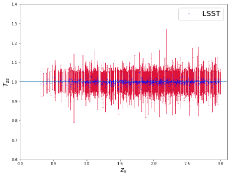
Figure 5: Individual measurements of the deviation of the SOL from the forthcoming LSST survey and WFIRST SNe Ia survey.

One the other hand, the Wide-Field InfraRed Space Telescope (WFIRST) is the future NASA mission, which presented a baseline six-year mission, including a two-year supernova survey strategy, corresponding to six months of “on-sky” time. There are about $10^{3}-10^{4}$ SNe Ia expected to be discovered (Hounsell et al., 2017). In order to create a realistic population of SN Ia sample we perform a Monte Carlo simulation in the following way: (1) we adopted the parameterized volumetric rate of SNe Ia as the number density of the SNe Ia population Rodney et al. (2014); Graur et al. (2014). In our simulation, a sample of 3000 SNe Ia covering the redshift range of $0.<z\leq 3.$ has been generated. (2) The peak rest-frame absolute magnitude $M_{B}$ obeys the gaussian distribution with a mean value of -19.3 mag and standard deviation of 0.2 mag, while the cross-filter $K$-corrections were computed from the one-component SNe Ia spectral template of Nugent et al. (2002) (please refer to Barbary (2014) for more details). (3) The total uncertainty budget for the distance modulus were presented in the Science Definition Team for WFIRST SN survey, which includes systematic uncertainty $\sigma_{sys}=0.01(1+z)/1.8$ mag (Hounsell et al., 2017), statistical measurement uncertainties and statistical model uncertainties $\sigma_{meas}=0.08$ mag (Spergel et al., 2015), the lensing uncertainty modeled as $\sigma_{lens}=0.07\times$ mag (Jönsson et al., 2010; Holz & Hughes, 2005), and intrinsic scatter $\sigma_{int}=0.09$ mag. Combining of the simulated strong lensing system from LSST and the simulated SN sample based on WFIRST and applying the redshift match, one can select 831 strong lensing systems which can be used to measure $c$ using our method. The expected individual results of the deviation of the SOL are shown in Fig. 5. Our results show that such a combination of strong lensing systems and SNe Ia will result in more stringent constraints for the deviation on the SOL at the level of $\Delta T_{zs}\sim 10^{-3}$ (corresponding to $\Delta c/c\sim 10^{-3}$) in the era of future missions.

4 Conclusions

In this work, we have proposed a new model-independent method to explore the deviation of the SOL at high redshift from the $c_{0}$ value known from laboratory measurements, by combining current largest SGL and SNe Ia sample. All the quantities that we need are given directly by observations. For a given SGL system, if the mass distribution is known, one can directly explore the deviation of the SOL by combining current SNe Ia observations acting as standard candle to provide distance information. In order to get the $D_{ls}/D_{s}$ distance ratio from SNe Ia acting as standard candles, we have used the assumption of spatial flatness in this work. However, compared with previous works, our method has the following advantages:

• Exploring the deviation of the SOL over a wide range of redshift instead of focusing on a single value of $z_{M}$ corresponding to the maximum of $D_{A}(z)$ function;

• Our method need not assume any cosmological model and the samples used here are also model-independent;

• The determination of the so called nuisance parameter $M_{B}$ of SNe Ia will be no longer necessary.

First of all, we turn to the recent catalog by Chen et al. (2019) that contains 161 SGL systems with source redshifts ranging from 0.197 to 3.595, obtained in four surveys including SLACS, BELLS, SL2S, and LSD. Combining these SGL systems together with the estimates of the angular diameter distances from standard candles (SNe Ia), we obtain the weighted average value $T_{zs}=0.983$ with the uncertainty $\Delta T_{zs}=0.013$ and median value $Med({T}_{zs})=0.980$ with the median absolute deviation $MAD({T}_{zs})=0.131$ for full sample, which indicate that the SOL at high redshifts is fully consistent with $c_{0}$ within uncertainty. There is no obvious evidence to support a deviation in the SOL in a distant Universe. The analysis of the SLACS sub-sample shows that there is no obvious deviation from the $c_{0}$ within 1$\sigma$ confidence region at low redshift range. For SL2S sub-sample, their deviation $T_{zs}>1$ can be a result of their systematics and incomplete samples. Thus, we may expect that the insufficient sample size will cause some deviations in the SOL. In order to show the full potential for our method, we also considered the simulated SGL systems from the forthcoming LSST survey combined with SNe Ia sample from the future WFIRST survey. Our results show that with these future surveys our approach of testing the deviation of the SOL may achieve constraints with much higher precision of $\Delta T_{zs}\sim 10^{-3}$.

In spite of the improved precision for testing the deviation of the SOL, there are several sources of systematic errors affecting our results, including the lens modeling, the uses of redshift matching criterion and the DDR. For the lens modeling, although the lens system has high resolution imaging at the current technique level, the uncertainty of stellar kinematic spectral observations of lens galaxies may lead to 10$\%$ statistical uncertainty in the measurement of the speed of light. Fortunately, in the coming optical imaging surveys, one can expect improved depth, area, resolution and the sharp increase in the number of SGL systems by the next generation of wide and deep sky surveys such as the Vera Rubin Observatory LSST survey (Collett, 2015; Shu et al., 2018). High-quality imaging and spectroscopic observations on SGL systems will certainly be very helpful to alleviate the problem. For redshift matching criterion, an interesting idea is to use lensed and unlensed type Ia supernovae (or other standardized sources) to estimate the speed of light (Cao et al., 2018) which can perfectly avoid systematic errors caused by the redshift match. For the use of the DDR, one can use alternative probes which directly provide the angular diameter distances to achieve testing the deviation of the SOL, such as ultra-compact radio structure acting standard rule (Cao et al., 2020).

As a final remark, any possible (statistically significant) deviation in the SOL might have profound implications for the understanding of fundamental physics and natural laws. This encourages us to look forward to the possible method to perform consistency testing for invariance of the speed of light on extragalactic objects with higher accuracy and precision in the future, which strengthens our interest in observational search for more SGL samples and astronomical probes with smaller statistical and systematic uncertainties.

Data Availability Statements

The data underlying this article will be shared on reasonable request to the corresponding author.

References

- Albrecht & Magueijo (1999) Albrecht, A., & Magueijo, J., 1999, PRD, 59, 043516
- Avelino & Martins (1999) Avelino, P. P., & Martins, C. J. A. P. 1999, PLB, 459, 468
- Auger et al. (2009) Auger, M. W., et al. 2009, ApJ, 705, 1099
- Auger et al. (2010) Auger, M. W., et al., 2010, ApJ, 724, 511
- Barbary (2014) Barbary, K. 2014, sncosmo v0.4.2, Zenodo, doi:10.5281/zenodo.11938
- Barrow (1999) Barrow, J. D. 1999, PRD, 59, 043515
- Bassett & Kunz (2004) Bassett, B. A., & Kunz, M. 2004, ApJ, 607, 661
- Bernstein (2006) Bernstein, G. 2006, ApJ, 637, 598
- Betoule et al. (2014) Betoule, M., et al. 2014, A&A, 568, 22
- Bevington et al. (1993) Bevington, P. R., et al. 1993, Computers in Physics 7, 415.
- Bolton et al. (2006) Bolton, A. S., Rappaport, S., & Burles, S. 2006, PRD, 74, 061501
- Bolton et al. (2008) Bolton, A. S., et al., 2008, ApJ, 682, 964
- Brownstein et al. (2015) Brownstein, J. R., et al., 2012, ApJ, 744, 41
- Cai et al. (2016) Cai, R. G., Guo, Z. K., & Yang, T. 2016, JCAP, 08, 016
- Cao & Liang (2011) Cao, S., & Liang, N. 2011, RAA, 11, 1199
- Cao et al. (2011b) Cao, S., Liang N., & Zhu, Z.-H. 2011, MNRAS, 416, 1099
- Cao et al. (2012) Cao, S., Pan, Y., Biesiada, M., Godłowski, W., & Zhu, Z.-H. 2012, JCAP, 03, 016
- Cao et al. (2015) Cao, S., Biesiada, M., Gavazzi, R., Piórkowska, A., & Zhu, Z.-H. 2015, ApJ, 806, 185
- Cao et al. (2016a) Cao, S., Biesiada, M., Yao, M., & Zhu, Z.-H. 2016a, MNRAS, 461, 2192
- Cao et al. (2016b) Cao, S., Biesiada, M., Zheng, X., & Zhu, Z.-H. 2016b, MNRAS, 457, 281
- Cao et al. (2017a) Cao, S., Biesiada, M., Jackson, J., Zheng, X., & Zhu, Z.-H. 2017a, JCAP, 02, 012
- Cao et al. (2017b) Cao, S., Li, X., Biesiada, M., et al. 2017b, ApJ, 835, 92
- Cao et al. (2018) Cao, S., Qi, J., Biesiada, M., et al. 2018, ApJ, 867, 50
- Cao et al. (2020) Cao, S., Qi, J., Biesiada, M., Liu, T., & Zhu, Z.-H. 2020, ApJL, 888, L25
- Chen et al. (2019) Chen, Y., Li, R., Shu, Y., & Cao. X. 2019, MNRAS, 488, 3745
- Clarkson, Bassett & Lu (2008) Clarkson, C., Bassett, B., & Lu, T. C. 2008, PRL, 101, 011301
- Collett (2015) Collett, T. E. 2015, ApJ, 811, 20
- Corasaniti (2006) Corasaniti, P. S. 2006, MNRAS, 372, 191
- Dicke (1957) Dicke, R. H. 1957, Reviews of Modern Physics, 29, 363
- Duff (2002) Duff, M.J., 2002 [arXiv:hep-th/0208093 ]
- Einstein (1907) Einstein, A. 1907, Jahrbuch der Radioaktivitat und Elektronik, 4, 411
- Ellis & Uzan (2005) Ellis, G. F. R., & Uzan, J.-P. 2005, Am. J. Phys. 73, 240
- Etherington (1933) Etherington, I. M. H. 1933, Phil. Mag, 15, 761
- Etherington (2007) Etherington, I. M. H. 2007, Gen. Rel. Grav, 39, 1055
- Feigelson & Babu (2012) Feigelson, E. & Babu G.J., Modern Statistical Methods for Astronomy: With R Applications, Cambridge University Press, Cambridge, 2012
- Freedman (2017) Freedman W. L. 2017, Nat. Astron, 1, 0169
- Gerhard et al. (2001) Gerhard O., Kronawitter A., Saglia R. P., & Bender R. 2001, AJ, 121, 1936
- Graur et al. (2014) Graur, O., et al. 2014, ApJ, 783, 28
- Grillo & Bertin (2014) Grillo, C., Lombardi, M., & Bertin, G. 2008, A&A, 477, 397
- Holz & Hughes (2005) Holz, D. E., & Hughes, S. A. 2005, ApJ, 629, 15
- Hounsell et al. (2017) Hounsell, R., Scolnic, D., Foley, R. J., et al. 2017, arXiv:1702.01747v1
- Jönsson et al. (2010) Jönsson, J., Sullivan, M., Hook, I., et al. 2010, MNRAS, 405, 535
- Kassiola & Kovner (1993) Kassiola, A. & Kovner, I. 1993, ApJ, 417, 450
- Kessler & Scolnic (2017) Kessler, R. & Scolnic, D. 2017, ApJ, 836, 56
- Koopmans & Treu (2002) Koopmans, L. V. E. & Treu, T. 2002, ApJ, 568, 5
- Koopmans & Treu (2003) Koopmans, L. V. E. & Treu, T. 2003, ApJ, 583, 606
- Koopmans (2005) Koopmans, L. V. E., 2006, EAS Publications Series, 20, 161
- Koopmans et al. (2006) Koopmans, L. V. E., Bolton, A. S., Burles, S. and Moustakas, L. A. 2006, ApJ, 649, 599
- Koopmans et al. (2009) Koopmans, L. V. E., Bolton, A., Treu, T., et al. 2009, ApJL, 703, L51
- Liu et al. (2019) Liu, T., Cao, S., Zhang, J., et al. 2019, ApJ, 886, 94
- Liu et al. (2020) Liu, T., Cao, S., Zhang, J., et al. 2020, MNRAS, 496, 708
- Ma et al. (2019) Ma, Y. B., Cao, S., Zhang, J., et al. 2019, EPJC, 79, 121
- Magueijo (2000) Magueijo, J. 2000, PRD, 62, 103521
- Magueijo (2003) Magueijo, J. 2003, Rept. Prog. Phys. 66, 2025
- Moffat (1993) Moffat, J. W. 1993, IJMPD, 2, 351
- Moffat (2002) Moffat, J. W. 2002 [arXiv:hep-th/0208109]
- Moffat (2016) Moffat, J. W. 2016, EPJC, 76, 130
- Navarro, Frenk & White (1997) Navarro, J. F., Frenk, C. S., & White, S. D. M. 1997, ApJ, 490, 493
- Nugent et al. (2002) Nugent, P., Kim, A., & Perlmutter, S. 2002, PASP, 114, 803
- Ofek et al. (2003) Ofek, E. O., Rix, H.-W., & Maoz, D. 2003, MNRAS, 343, 639
- Petit (1988) Petit, J. P. 1988, MPLA, 3, 1527
- Perlmutter et al. (1999) Perlmutter, S., et al. 1999, ApJ, 517, 565
- Planck Collaboration (2018) Aghanim, N., Akrami, Y., Ashdown, M., et al. 2018, arXiv:1807.06209
- Qi et al. (2014) Qi, J., Zhang, M., & Liu, W. 2014, PRD, 90, 063526
- Qi et al. (2018) Qi, J., Cao, S., Biesiada, M., & Zhu Z.-H. 2018, RAA, 18, 66
- Qi et al. (2019) Qi, J., et al. 2019, MNRAS, 483, 1
- Räsänen, et al. (2015) Rsnen, S., Bolejko, K., & Finoguenov, A. 2015, PRL, 115, 101301
- Rest et al. (2014) Rest, A., Scolnic, D., Foley, R. J., et al. 2014, ApJ, 795, 44
- Riess et al. (1998) Riess, A. G., et al. 1998, AJ, 116, 1009
- Rix & White (1992) Rix, H. W., & White, S. D. M. 1992, MNRAS, 254, 389
- Rodney et al. (2014) Rodney, S. A., et al., 2014, AJ, 148, 13
- Ruff et al. (2011) Ruff, A. J., et al., 2011, ApJ, 727, 96
- Rusin & Kochanek (2005) Rusin, D. & Kochanek, C. S. 2005, ApJ, 623, 666
- Salzano, Da̧browski & Lazkoz (2015) Salzano, V., Da̧browski, M., & Lazkoz, R. 2015, PRL, 114, 101304
- Salzano, Da̧browski & Lazkoz (2016) Salzano, V., Da̧browski, M., & Lazkoz, R. 2016, PRD, 93, 063521
- Salzano (2017) Salzano, V. 2017, PRD, 95, 084035
- Schwab et al. (2009) Schwab J., Bolton A. S., Rappaport S. A., 2009, ApJ, 708, 750
- Schwab et al. (2010) Schwab, J., Bolton, A. S., & Rappaport, S. A. 2010, ApJ, 708, 750
- Scolnic et al. (2014) Scolnic, D., Rest, A., Riess, A., et al. 2014, ApJ, 795, 45
- Scolnic et al. (2018) Scolnic, D., et al. 2018, ApJ, 859, 101
- Seikel, Clarkson & Smith (2012) Seikel, M., Clarkson, C., & Smith, M. 2012, JCAP, 06, 036
- Sérsic (1968) Sérsic, J. L., 1968, Atlas de galaxias australes Cordoba, Argentina: Observatorio Astronomico
- Shu et al. (2015) Shu, Y., et al. 2015, ApJ, 803, 71
- Shu et al. (2016a) Shu, Y., et al. 2016a, ApJ, 824, 86
- Shu et al. (2016b) Shu, Y., et al. 2016b, ApJ, 833, 264
- Shu et al. (2017) Shu, Y., et al. 2017, ApJ, 851, 48
- Shu et al. (2018) Shu, Y., et al. 2018, ApJ, 864,91
- Sonnenfeld et al. (2013a) Sonnenfeld, A., et al. 2013a, ApJ, 777, 98
- Sonnenfeld et al. (2013b) Sonnenfeld, A., et al. 2013b, ApJ, 777, 97
- Sonnenfeld et al. (2015) Sonnenfeld, A., et al. 2015, ApJ, 800, 94
- Spergel et al. (2015) Spergel, D., Gehrels, N., Baltay, C., et al. 2015, arXiv:1503.03757
- Treu & Koopmans (2002) Treu, T. and Koopmans, L. V. E. 2002, ApJ, 575, 87.
- Treu & Koopmans (2004) Treu, T. and Koopmans, L. V. E. 2004, ApJ, 611, 739.
- Treu et al. (2006) Treu, T., Koopmans, L. V. E., Bolton, A. S., Burles, S., & Moustakas, L. A. 2006, ApJ, 650, 1219
- Valentino, Anchordoqui & Akarsu (2020) Valentino, E. D., Anchordoqui and L. A., Akarsu, O. 2020, arXiv:2008.11284
- Valentino, Melchiorri & Silk (2019) Valentino, E. D., Melchiorri, A., & Silk, J. 2019, Nat. Astron, 4, 196
- van Dokkum & Stanford (2003) van Dokkum, P. G., & Stanford, S. A. 2003, ApJ, 585, 78
- Wang et al. (2019) Wang, D. D., Zhang, H. Y., Zheng, J, L., et al. 2019, arXiv:1904.04041
- Xia et al. (2017) Xia, J.-Q., et al. 2017, ApJ, 834, 75
- Zheng et al. (2016) Zheng, X. G., Ding, X. H., Biesiada, M., Cao, S., & Zhu, Z. H. 2016, ApJ, 825, 17
- Zheng et al. (2018) Zheng, X. G., Biesiada, M., Ding, X. H., Cao, S., Zhang, S. X., & Zhu, Z. H. 2018, EPJC, 78, 274