GTMD model predictions for diffractive dijet production at EIC

Abstract

In this paper we consider a small-$x$ model for gluon GTMDs that we fit to data on diffractive dijet production in electron-proton collisions obtained by HERA’s H1 Collaboration. Assuming a small number of free parameters, each with a physical motivation, we are able to describe those data fairly well and with this model we obtain predictions for the EIC for both electroproduction and photoproduction which may allow to further test the underlying GTMD description. In the general discussion of the impact parameter dependence we recall some subtle issues related to localization of states, choice of frames, and discuss what these aspects imply for the range of applicability of the model.

I Introduction

Generalized Transverse Momentum Dependent parton distributions (GTMDs) and the associated Wigner parton distributions were first considered in Ji:2003ak ; Belitsky:2003nz and analyzed further in e.g. Meissner:2008ay ; Meissner:2009ww ; Lorce:2011dv ; Echevarria:2016mrc for quarks and in Echevarria:2016mrc ; More:2017zqp for gluons. The first suggestion to access GTMDs experimentally was put forward in Hatta:2016dxp . In that paper the process of diffractive dijet production in electron-proton collisions was considered to probe gluon GTMDs. Diffractive dijet production was earlier suggested as a way to probe gluon Generalized Parton Distributions (GPDs) Braun:2005rg and considered at small $x$ in Altinoluk:2015dpi . Diffractive single jet production was studied in Peccini:2020tpj . In the present paper we follow up on these ideas and construct a model for the unpolarized gluon GTMD similar to the one put forward in Hatta:2016dxp . Models for quark GTMDs have been considered in e.g. Kaur:2019kpi ; Luo:2020yqj ; Zhang:2020ecj . For gluon GTMDs the models are so-far based on the small-$x$ McLerran-Venugopalan (MV) model McLerran:1993ni ; McLerran:1993ka ; McLerran:1994vd and related Color Glass Condensate (CGC) descriptions. We will also take the MV model as our starting point, but introduce a few free parameters to be fitted to H1 data from the HERA collider in order to arrive at predictions for the U.S.-based Electron-Ion Collider (EIC) that hopefully will allow to further test the underlying GTMD description. We will only consider unpolarized gluons, because the azimuthal modulations in the diffractive dijet cross section arising from the elliptic GTMD Hatta:2016dxp ; Zhou:2016rnt are expected to be much smaller than the present cross section uncertainties. In the model studies of Hagiwara:2016kam ; Hagiwara:2017fye ; Mantysaari:2019csc ; Salazar:2019ncp ; Hatta:2020bgy and in the CMS data CMS:2020ekd the azimuthal asymmetries are found to be at the 10-30% level or (much) smaller. As a first step it would be important to check whether the GTMD description of diffractive dijet production is consistent with cross section measurements in various kinematic variables and various kinematic regions. With the presented results we hope to facilitate such a study.

This paper is organized as follows. In section II we discuss the definitions and properties of GTMDs in general and recall some subtle issues regarding the localization of states and the impact parameter dependence. In section III we discuss the model and its free parameters, addressing also the range of applicability of the model. We furthermore argue that the process of diffractive dijet production in electron-proton collisions in the so-called correlation limit falls within that range. In section IV we provide details on the cross section calculation in terms of the unpolarized gluon GTMD. We discuss the fit of our model to H1 data in section V and present our predictions for the EIC in section VI. We end with a concluding section.

II Definitions of GTMDs

GTMDs are 5-dimensional parton distributions that depend on the parton’s lightcone momentum fraction $x$, the parton’s transverse momentum $\bm{k}_{\perp}$ and the transverse off-forwardness $\Delta_{\perp}$ by which the incoming hadron momentum gets modified. The associated Wigner distribution parton is a function of $x$, $\bm{k}_{\perp}$, and the impact parameter $\bm{b}_{\perp}$ which is the Fourier conjugate of $\bm{\Delta}_{\perp}$. GTMDs can be viewed as off-forward extensions of Transverse Momentum Dependent parton distributions (TMDs) or as transverse momentum dependent extensions of GPDs. As a consequence, the GTMDs inherit properties of both TMDs and GPDs and any subtle issues related to them. In this section we will go into some of these matters, restricting the discussion to the distribution of unpolarized quarks inside an unpolarized hadron, for which we take a proton for definiteness.

First of all, the quark GTMD $q(x,\bm{k}_{\perp},\bm{\Delta}_{\perp})$ can be defined as the off-forward generalization of the quark TMD $q(x,\bm{k}_{\perp})$:

$$q(x,\bm{k}_{\perp},\bm{\Delta}_{\perp}) \equiv\int\frac{d\lambda}{2\pi P^{+}}\,d^{2}\bm{r}_{\perp}\,e^{i\lambda x}e^{i\bm{k}_{\perp}\cdot\bm{r}_{\perp}}\,\langle{P^{\prime}}|\;{\overline{\psi}(-\frac{\lambda}{2}n-\frac{\bm{r}_{\perp}}{2})\,\gamma^{+}{\cal L}\,\psi(\frac{\lambda}{2}n+\frac{\bm{r}_{\perp}}{2})}\;|{P}\rangle,$$ (1)

where the lightlike vector $n$ specifies the $-$ direction, whereas the proton momentum $P$ specifies the $+$ direction: $P\cdot n=P^{+}$. In the above expression $\Delta=P^{\prime}-P$ denotes the off-forwardness considered here for zero skewness, i.e. $\xi=-\Delta^{+}/({P^{\prime}}^{+}+P^{+})=0$ and $\Delta=\Delta_{\perp}$. The path-ordered exponential or gauge link ${\cal L}$ does not play an important role here and will be left unspecified.

Alternatively, the quark GTMD can be defined as the Fourier transform of the Wigner quark distribution $W(x,\bm{k}_{\perp},\bm{b}_{\perp})$, which itself can be defined as the transverse momentum dependent generalization of the impact parameter dependent GPD $q(x,\bm{b}_{\perp})$ Soper:1976jc ; Burkardt:2000za ; Diehl:2002he ; Burkardt:2002hr ; Burkardt:2002ks :

$$q(x,\bm{b}_{\perp})=\int\frac{d\lambda}{2\pi P^{+}}\,e^{i\lambda x}\,\langle{P^{+},\bm{R}_{\perp}=0}|\;\overline{\psi}(-\frac{\lambda}{2}n+{\bm{b}_{\perp}})\,\gamma^{+}\,{\cal L}\,\psi(\frac{\lambda}{2}n+{\bm{b}_{\perp}})\;|{P^{+},\bm{R}_{\perp}=0}\rangle,$$ (2)

where the impact parameter $\bm{b}_{\perp}$ is measured w.r.t. the transverse center of longitudinal momentum $\bm{R}_{\perp}^{CM}\equiv\sum_{i}x_{i}\bm{r}_{\perp i}$ of the system and $|{P^{+},\bm{R}_{\perp}=0}\rangle$ is the normalized proton state localized in the spatial $\perp$ direction Diehl:2002he ; Burkardt:2002ks :

$$|{P^{+},\bm{R}_{\perp}=0}\rangle={\cal N}\int\frac{d^{2}\bm{P}_{\perp}}{(2\pi)^{2}}\Phi(\bm{P}_{\perp})|P^{+},\bm{P}_{\perp}\rangle,$$ (3)

for some wave packet $\Phi(\bm{P}_{\perp})$. This expression for $q(x,\bm{b}_{\perp})$ thus depends on the wave packet considered. If this wave packet is sufficiently localized in transverse position space, such that $\Phi(\bm{P}_{\perp}+\bm{\Delta}_{\perp})\approx\Phi(\bm{P}_{\perp})$, meaning it is slowly varying on the scale of the off-forwardness, one can relate it to the standard GPD $H$ Burkardt:2000za ; Diehl:2002he ; Burkardt:2002hr ; Burkardt:2002ks :

$$q(x,\bm{b}_{\perp}) =|{\cal N}|^{2}\int\frac{d\lambda}{2\pi P^{+}}\,e^{i\lambda x}\int\frac{d^{2}\bm{P}_{\perp}}{(2\pi)^{2}}\frac{d^{2}\bm{P}^{\prime}_{\perp}}{(2\pi)^{2}}\,\Phi^{*}(\bm{P}^{\prime}_{\perp})\Phi(\bm{P}_{\perp})\langle{P^{+},\bm{P}^{\prime}_{\perp}}|\;\overline{\psi}(-\frac{\lambda}{2}n+{\bm{b}_{\perp}})\,\gamma^{+}\,{\cal L}\,\psi(\frac{\lambda}{2}n+{\bm{b}_{\perp}})\;|{P^{+},\bm{P}_{\perp}}\rangle$$

$$=|{\cal N}|^{2}\int\frac{d\lambda}{2\pi P^{+}}\,e^{i\lambda x}\int\frac{d^{2}\bm{P}_{\perp}}{(2\pi)^{2}}\frac{d^{2}\bm{P}^{\prime}_{\perp}}{(2\pi)^{2}}\,\Phi^{*}(\bm{P}^{\prime}_{\perp})\Phi(\bm{P}_{\perp})e^{-i\bm{b}_{\perp}\cdot\bm{\Delta}_{\perp}}\langle{P^{+},\bm{P}^{\prime}_{\perp}}|\;\overline{\psi}(-\frac{\lambda}{2}n)\,\gamma^{+}\,{\cal L}\,\psi(\frac{\lambda}{2}n)\;|{P^{+},\bm{P}_{\perp}}\rangle$$

$$\approx|{\cal N}|^{2}\int\frac{d^{2}\bm{P}_{\perp}}{(2\pi)^{2}}|\Phi(\bm{P}_{\perp})|^{2}\frac{d^{2}\bm{\Delta}_{\perp}}{(2\pi)^{2}}\,e^{-i\bm{b}_{\perp}\cdot\bm{\Delta}_{\perp}}H(x,0,-\bm{\Delta}^{2}_{\perp})=\int\frac{d^{2}\bm{\Delta}_{\perp}}{(2\pi)^{2}}\,e^{-i\bm{b}_{\perp}\cdot\bm{\Delta}_{\perp}}H(x,0,-\bm{\Delta}^{2}_{\perp}).$$ (4)

In the second step we used that, unlike forward matrix elements, off-forward matrix elements of the form $\langle{P^{+},\bm{P}^{\prime}_{\perp}}|\;O(\bm{b}_{\perp})\;|{P^{+},\bm{P}_{\perp}}\rangle$ are not translation invariant, but pick up a phase when translating the operator $O(\bm{b}_{\perp})$ to $O(\bm{0}_{\perp})$. In the above derivation it was also used that $\langle P^{+},\bm{P}^{\prime}_{\perp}|\;O(\bm{0}_{\perp})\;|P^{+},\bm{P}_{\perp}\rangle$ only depends on the difference of $\bm{P}^{\prime}_{\perp}$ and $\bm{P}_{\perp}$, which is a consequence of invariance under transverse boosts, see Diehl:2002he , in particular its Eq. (5).

One observes that only in the case that $\Phi(\bm{P}_{\perp})$ is a constant, the relation between $q(x,\bm{b}_{\perp})$ and $H(x,0,-\bm{\Delta}^{2}_{\perp})$ is exact. When viewing $q(x,\bm{b}_{\perp})$ as the Fourier transform of the GPD $H(x,0,-\bm{\Delta}^{2}_{\perp})$ it is thus understood that one considers a wave packet that is sufficiently localized in coordinate space and hence sufficiently delocalized in momentum space. This then raises the question of how to reconcile such a very delocalized state in transverse momentum space with a state that has a specific $z$-momentum and energy, which are related by $P^{-}=(M^{2}+P_{\perp}^{2})/(2P^{+})$. This issue is known to pose a problem for 3D spatial distributions, where a state cannot be simultaneously in a definite eigenstate of position and momentum and frame and wave packet dependence enters. For the 2D charge distribution and analogously for $q(x,\bm{b}_{\perp})$ one can avoid this issue by boosting to a frame in which $P^{+}$ is much larger than the typical $P_{\perp}$ values. This allows to maintain $P^{-}=(M^{2}+P_{\perp}^{2})/(2P^{+})\ll P^{+}$ in the wave packet, such that the state has sufficiently definite $P^{0}$ and $P^{3}$ components even if the $P_{\perp}$ distribution is very broad, cf. Diehl:2002he for further discussion.

Starting from the impact parameter dependent GPD $q(x,\bm{b}_{\perp})$ one obtains a definition of the Wigner parton distribution $W(x,\bm{k}_{\perp},\bm{b}_{\perp})$ defined as

$$W(x,\bm{k}_{\perp},\bm{b}_{\perp})\equiv\int\frac{d\lambda}{2\pi P^{+}}\,d^{2}\bm{r}_{\perp}\,e^{i\lambda x}e^{i\bm{k}_{\perp}\cdot\bm{r}_{\perp}}\,\langle{P^{+},\bm{R}_{\perp}=0}|\;\overline{\psi}(-\frac{\lambda}{2}n+{\bm{b}_{\perp}}-\frac{\bm{r}_{\perp}}{2})\,\gamma^{+}\,{\cal L}\,\psi(\frac{\lambda}{2}n+{\bm{b}_{\perp}}+\frac{\bm{r}_{\perp}}{2})\;|{P^{+},\bm{R}_{\perp}=0}\rangle.$$ (5)

The GTMD is then defined as

$$q_{W}(x,\bm{k}_{\perp},\bm{\Delta}_{\perp}) \equiv\int\frac{d^{2}\bm{b}_{\perp}}{(2\pi)^{2}}\,e^{i\bm{b}_{\perp}\cdot\bm{\Delta}_{\perp}}W(x,\bm{k}_{\perp},\bm{b}_{\perp}).$$ (6)

Just like for the Fourier transform of $q(x,\bm{b}_{\perp})$ and the GPD $H(x,0,-\bm{\Delta}^{2}_{\perp})$, one can equate the two GTMD definitions Eqs. (1) and (6) for a sufficiently narrow state $|{P^{+},\bm{R}_{\perp}=0}\rangle$ in coordinate space, for which, as we discussed above, one has to consider a frame in which $P^{+}$ is much larger than the typical $P_{\perp}$ values. We emphasize that the sufficiently narrow state refers to the wave packet in which the state is prepared, not to the nucleon or nucleus which itself will have some profile in transverse coordinate space that may be considerably less narrow.

When one considers small $x$ values gluons dominate, hence we will from now focus on (unpolarized) gluon distributions. More specifically, the process of diffractive dijet production in electron-proton or electron-nucleus collisions probes the dipole gluon GTMD (again considered for zero skewness) defined as Hatta:2016dxp ; Boer:2018vdi :

$$G^{[+,-]}(x,\bm{k}_{\perp},\bm{\Delta}_{\perp})=\frac{2}{P^{+}}\int\frac{dz^{-}}{2\pi}\frac{d^{2}\bm{z}_{\perp}}{(2\pi)^{2}}\,e^{ik\cdot z}\left.\langle{P^{\prime}}|\;{\rm Tr}\left[F^{+i}\left(-\frac{z}{2}\right)U^{[+]}F^{+i}\left(\frac{z}{2}\right)U^{[-]}\right]\;|{P}\rangle\right|_{z^{+}=0}.$$ (7)

Here $i$ is a transverse index that is summed over in this case of unpolarized gluons and $U^{[\pm]}$ are the standard staple-like gauge links in the forward ($+$) and backward ($-$) lightcone directions, also simply referred to as $+$ and $-$ links. The function $xG_{{\rm DP}}(x,\bm{q}_{\perp},\bm{\Delta}_{\perp})$ in Hatta:2016dxp corresponds to $G^{[+,-]}(x,\bm{q}_{\perp},\bm{\Delta}_{\perp})$.

In the limit of $x\to 0$ one can show to arrive at Boer:2018vdi

$$G^{[+,-]}(\bm{k}_{\perp},\bm{\Delta}_{\perp}) =\frac{4}{g^{2}\langle P|P\rangle}\int\frac{d^{2}\bm{x}_{\perp}d^{2}\bm{y}_{\perp}}{(2\pi)^{3}}\,e^{-i\bm{k}_{\perp}\cdot(\bm{x}_{\perp}-\bm{y}_{\perp})}e^{i\bm{\Delta}_{\perp}\cdot(\bm{x}_{\perp}+\bm{y}_{\perp})/2}\langle{P^{\prime}}|\;\partial^{i}_{x}\partial^{i}_{y}{\rm Tr}\left[U^{[\Box]}(\bm{y}_{\perp},\bm{x}_{\perp})\right]\;|{P}\rangle$$

$$\equiv\frac{1}{2\pi g^{2}}\left[\bm{k}_{\perp}^{2}-\frac{\bm{\Delta}_{\perp}^{2}}{4}\right]G^{[\Box]}(\bm{k}_{\perp},\bm{\Delta}_{\perp}),$$ (8)

where $U^{[\Box]}(\bm{y}_{\perp},\bm{x}_{\perp})=U^{[+]}(\bm{y}_{\perp},\bm{x}_{\perp})U^{[-]}(\bm{x}_{\perp},\bm{y}_{\perp})$ will be referred to as the Wilson loop and $\langle P^{\prime}|P\rangle=(2\pi)^{3}2P^{+}\delta(\Delta^{+})\delta^{(2)}(\Delta_{\perp})$ yielding the divergent factor $\langle P|P\rangle=2P^{+}\int db^{-}d^{2}\bm{b}_{\perp}$, which is assumed to be regularized, e.g.  by considering a finite volume. In this way one finds that

$$G^{[\Box]}(\bm{k}_{\perp},\bm{\Delta}_{\perp}) =\frac{4N_{c}}{\langle P|P\rangle}\int\frac{d^{2}\bm{x}_{\perp}d^{2}\bm{y}_{\perp}}{(2\pi)^{2}}\,e^{-ik\cdot(\bm{x}_{\perp}-\bm{y}_{\perp})}e^{i\Delta\cdot(\bm{x}_{\perp}+\bm{y}_{\perp})/2}\langle{P^{\prime}}|\;S^{[\Box]}(\bm{x}_{\perp},\bm{y}_{\perp})\;|{P}\rangle$$

$$=\frac{4N_{c}}{\langle P|P\rangle}\int\frac{d^{2}\bm{r}_{\perp}d^{2}\bm{b}_{\perp}}{(2\pi)^{2}}\,e^{-i\bm{k}_{\perp}\cdot\bm{r}_{\perp}}e^{i\bm{\Delta}_{\perp}\cdot\bm{b}_{\perp}}\langle{P^{\prime}}|\;S^{[\Box]}(\bm{b}_{\perp}-\frac{\bm{r}_{\perp}}{2},\bm{b}_{\perp}+\frac{\bm{r}_{\perp}}{2})\;|{P}\rangle$$ (9)

where $S^{[\Box]}(\bm{x}_{\perp},\bm{y}_{\perp})\equiv{\rm Tr}\left[U^{[\Box]}(\bm{y}_{\perp},\bm{x}_{\perp})\right]/N_{c}$, $\bm{r}_{\perp}=\bm{y}_{\perp}-\bm{x}_{\perp}$ and $\bm{b}_{\perp}=(\bm{x}_{\perp}+\bm{y}_{\perp})/2$. Comparing again to the notation of Hatta:2016dxp we see that ${\cal F}_{x}=G^{[\Box]}/((4\pi)^{2}N_{c})$, where ${\cal F}_{x}$ satisfies the normalization condition $\int d^{2}\bm{k}_{\perp}\,d^{2}\bm{\Delta}_{\perp}\,e^{-i\bm{\Delta}_{\perp}\cdot\bm{b}_{\perp}}\,{\cal F}_{x}(\bm{k}_{\perp},\bm{\Delta}_{\perp})=1$. In Eq. (9) $\bm{b}_{\perp}$ is defined w.r.t. some unspecified reference point, so one may wonder what determines this position? In fact, in the derivation of Eq. (8) the following step is performed:

$$\langle P+\Delta_{\perp}|O(\bm{0}_{\perp},\bm{r}_{\perp})|P\rangle=e^{i\bm{b}_{\perp}\cdot\bm{\Delta}_{\perp}}\langle P+\Delta_{\perp}|O(\bm{b}_{\perp},\bm{r}_{\perp})|P\rangle=\frac{\int d^{2}\bm{b}_{\perp}e^{i\bm{b}_{\perp}\cdot\bm{\Delta}_{\perp}}\langle P+\Delta_{\perp}|O(\bm{b}_{\perp},\bm{r}_{\perp})|P\rangle}{\int d^{2}\bm{b}_{\perp}},$$ (10)

where the last step is formally exact, but as mentioned, the normalization factor $\int d^{2}\bm{b}_{\perp}$ (which is part of $\langle P|P\rangle$) is actually divergent and requires consideration of a regulator. In the derivation it is used that although matrix elements of the form $\langle P+\Delta_{\perp}|O(\bm{b}_{\perp})|P\rangle$ are both $\bm{b}_{\perp}$ and $\bm{\Delta}_{\perp}$ dependent, despite $\bm{b}_{\perp}$ and $\bm{\Delta}_{\perp}$ being each other’s Fourier conjugates, the $\bm{b}_{\perp}$ dependence enters just through a phase. As a result, the integrand is actually $\bm{b}_{\perp}$ independent and any reference point will do. However, the previous GPD analysis suggests that it is better to replace Eq. (10) by

$$\langle P+\Delta_{\perp}|O(\bm{0}_{\perp},\bm{r}_{\perp})|P\rangle=\int\frac{d^{2}\bm{b}_{\perp}}{(2\pi)^{2}}\,e^{i\bm{b}_{\perp}\cdot\bm{\Delta}_{\perp}}\langle P^{+},\bm{R}_{\perp}=0|O(\bm{b}_{\perp},\bm{r}_{\perp})|P^{+},\bm{R}_{\perp}=0\rangle,$$ (11)

where $\bm{b}_{\perp}$ is considered w.r.t. $\bm{R}_{\perp}=0$ and a large $P^{+}$ momentum frame and a spatially localized wave packet are implicitly considered. It is also implicitly used that $\langle{P^{+},\bm{P}^{\prime}_{\perp}}|\;O(\bm{0}_{\perp},\bm{r}_{\perp})\;|{P^{+},\bm{P}_{\perp}}\rangle$ only depends on the difference of $\bm{P}^{\prime}_{\perp}$ and $\bm{P}_{\perp}$, just like for $\bm{r}_{\perp}=0$ in the GPD case ($\bm{r}_{\perp}$ is not affected by the required transverse boosts, since the corresponding $r^{+}=0$). It is furthermore interesting to note that Eq. (11) relates an off-forward matrix element to an integral over diagonal matrix elements.

Following the above replacement, matrix elements of the form $\langle P^{\prime}|O(\bm{b}_{\perp},\bm{r}_{\perp})|{P}\rangle/\langle P|P\rangle$ are to be interpreted as $\langle P^{+},\bm{R}_{\perp}=0|O(\bm{b}_{\perp},\bm{r}_{\perp})|P^{+},\bm{R}_{\perp}=0\rangle$ in the expression for $G^{[\Box]}$ and, similarly, for ${\cal F}^{[\Box]}$ which follows from $G^{[\Box]}$ by the replacement $S^{[\Box]}(\bm{x}_{\perp},\bm{y}_{\perp})\to 1-S^{[\Box]}(\bm{x}_{\perp},\bm{y}_{\perp})$:

$${\cal F}^{[\Box]}(\bm{k}_{\perp},\bm{\Delta}_{\perp}) =\frac{4N_{c}}{\langle P|P\rangle}\int\frac{d^{2}\bm{x}_{\perp}d^{2}\bm{y}_{\perp}}{(2\pi)^{2}}\,e^{-ik\cdot(\bm{x}_{\perp}-\bm{y}_{\perp})}e^{i\Delta\cdot(\bm{x}_{\perp}+\bm{y}_{\perp})/2}\langle{P^{\prime}}|\;1-S^{[\Box]}(\bm{x}_{\perp},\bm{y}_{\perp})\;|{P}\rangle$$

$$=\frac{4N_{c}}{\langle P|P\rangle}\int\frac{d^{2}\bm{r}_{\perp}d^{2}\bm{b}_{\perp}}{(2\pi)^{2}}\,e^{-i\bm{k}_{\perp}\cdot\bm{r}_{\perp}}e^{i\bm{\Delta}_{\perp}\cdot\bm{b}_{\perp}}\langle{P^{\prime}}|\;1-S^{[\Box]}(\bm{b}_{\perp}-\frac{\bm{r}_{\perp}}{2},\bm{b}_{\perp}+\frac{\bm{r}_{\perp}}{2})\;|{P}\rangle.$$ (12)

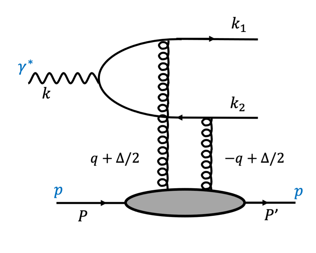
Figure 1: One of the leading order diagrams of diffractive dijet production in $ep$ collisions.

Following Ref. Hatta:2016dxp the cross section of diffractive dijet production in electron-proton collisions is expressed in terms of ${\cal F}^{[\Box]}$ as

$$\frac{d\sigma}{dy_{1}dy_{2}d^{2}\bm{k}_{1\perp}d^{2}\bm{k}_{2\perp}}\propto\int d^{2}\bm{q}_{\perp}d^{2}\bm{q}^{\prime}_{\perp}{\cal F}^{[\Box]}(\bm{q}_{\perp},\bm{\Delta}_{\perp}){\cal F}^{[\Box]}(\bm{q}^{\prime}_{\perp},\bm{\Delta}_{\perp}){\cal A}(\bm{K}_{\perp},\bm{q}_{\perp},\bm{q}^{\prime}_{\perp},\epsilon_{f}^{2}),$$ (13)

for a particular amplitude function ${\cal A}$. Here $K_{\perp}$ is the transverse part of $K=(k_{1}-k_{2})/2$, where $k_{i}$ denotes the momentum of jet $i$, $\Delta_{\perp}$ is the transverse part of $\Delta=k_{1}+k_{2}$, $y_{i}$ is the rapidity of jet $i$, and $\epsilon_{f}^{2}=z(1-z)Q^{2}$, with $z$ is the momentum fraction of one of the two jets. One considers this process in the so-called correlation limit: $\Delta_{\perp}\ll K_{\perp}$, where $K_{\perp}$ sets the hard scale, allowing to also consider the photoproduction ($Q^{2}=0$) case. One of the leading order diagrams of diffractive dijet production in $ep$ collisions in this kinematic regime is shown in Fig. 1. In this exclusive process the transverse momentum of the jet pair gives a handle on the $\bm{\Delta}_{\perp}$ momentum, even if the off-forwardness of the struck nucleon or nucleus itself is not measured. More details of the cross section calculation will be given below, but first we will discuss the model for the Wilson loop GTMD $G^{[\Box]}$ and the corresponding ${\cal F}^{[\Box]}$.

III Model for the unpolarized gluon GTMD at small $x$

In the process considered the incoming virtual photon splits into a quark-antiquark dipole pair that interacts with the proton or nucleus.. The large jet transverse momentum, or equivalently large $K_{\perp}$, the typical size $r_{\perp}$ of the dipole will be small. At small enough $x$ even small dipoles will have multiple interactions with the target. In the saturation regime at small $x$ one often employs the McLerran-Venugopalan (MV) model for the dipole scattering amplitude McLerran:1993ni ; McLerran:1993ka ; McLerran:1994vd ; Gelis:2001da ; Gelis:2010nm :

$$\left\langle\frac{S^{[\Box]}(\bm{x}_{\perp},\bm{y}_{\perp})+S^{[\Box]\dagger}(\bm{x}_{\perp},\bm{y}_{\perp})}{2}\right\rangle_{C}=\exp\left(-\frac{1}{4}{r}_{\perp}^{2}Q_{s}^{2}\ln\left[\frac{1}{{r_{\perp}^{2}}\Lambda^{2}}+e\right]\right),$$ (14)

where the subscript $C$ indicates that an average over the color configuration of the target is taken, $\Lambda$ denotes the QCD scale, and $e$ is the natural number. For an infinitely large nuclear target the saturation scale $Q_{s}$ is only a function of $x$. As a consequence, in that case the MV model expression applies to the forward scattering case and it is only a function of $\bm{r}_{\perp}=\bm{y}_{\perp}-\bm{x}_{\perp}$ due to translational invariance ($r_{\perp}^{2}=|\bm{r}_{\perp}^{2}|$). For finite nuclei at small $x$, a dependence of $Q_{s}$ on impact parameter is often considered, see e.g. Mueller:1989st ; GolecBiernat:2003ym ; Iancu:2017fzn . The $b_{\perp}(=|\bm{b}_{\perp}|)$ dependence of $Q_{s}$ is usually implemented as $Q_{s}^{2}(x,b_{\perp})\equiv Q_{s}^{2}(x)T_{A}(b_{\perp})$, where $T_{A}(b_{\perp})$ is the nuclear profile function or nuclear thickness function that describes the distribution of nuclear matter inside a nucleus integrated over the $z$ component of $\bm{b}$ Iancu:2017fzn . Here $T_{A}(b_{\perp})$ scales with $A^{1/3}$. For scattering off a proton at very small $x$ that is described by the CGC, one can similarly introduce a profile function. To be specific, we will consider

$$Q_{s}^{2}({b}_{\perp})=\frac{4\pi\alpha_{s}^{2}C_{F}}{N_{c}}T_{p}({b}_{\perp}),$$ (15)

with a Gaussian ${b}_{\perp}$ profile Salazar:2019ncp :

$$T_{p}(b_{\perp})=\exp\left(-b_{\perp}^{2}/(2R_{p}^{2})\right),$$ (16)

where $R_{p}$ is the gluonic radius of the proton for which we will take the value $R_{p}=0.5\ \text{fm}$, such that $1/R_{p}\approx 0.4$ GeV.

Using Eq. (14) with this $Q_{s}^{2}({b}_{\perp})$ implies automatically nonzero off-forwardness, even if one is considering only diagonal expectation values. Furthermore, by identifying (and implicitly absorbing the lightcone volume factor $2P^{+}\int db^{-}$ of $\langle P|P\rangle$ in the process)

$$\langle S^{[\Box]}(\bm{b}_{\perp},\bm{r}_{\perp})\rangle_{C}=\langle P^{+},\bm{R}_{\perp}=0|S^{[\Box]}(\bm{b}_{\perp},\bm{r}_{\perp})|P^{+},\bm{R}_{\perp}=0\rangle,$$ (17)

we arrive at the following expression for the GTMD:

$$G^{[\Box]}(\bm{k}_{\perp},\bm{\Delta}_{\perp}) =4N_{c}\int\frac{d^{2}\bm{r}_{\perp}d^{2}\bm{b}_{\perp}}{(2\pi)^{2}}\,e^{-i\bm{k}_{\perp}\cdot\bm{r}_{\perp}}e^{i\bm{\Delta}_{\perp}\cdot\bm{b}_{\perp}}\exp\left(-\frac{1}{4}{r}_{\perp}^{2}Q_{s}^{2}(b_{\perp})\ln\left[\frac{1}{{r}_{\perp}^{2}\Lambda^{2}}+e\right]\right).$$ (18)

This becomes the standard MV model expression for the gluon TMD in the limit $R_{p}\to\infty$ and $\Delta_{\perp}\to 0$. We expect this model expression to be applicable as long as the typical $b_{\perp}$ values probed are larger than the typical dipole sizes. Therefore, we will restrict application of the model to the region $\Delta_{\perp}\raisebox{-4.0pt}{$\,\stackrel{{\scriptstyle\textstyle<}}{{\sim}}\,$}1$ GeV, which is consistent with the correlation limit, because well-defined jets will have transverse momenta of at least a few GeV. In practice, higher $\Delta_{\perp}$ will hardly matter, as will be seen (cf. Fig. 3).

In Hagiwara:2016kam ; Hagiwara:2017fye Gaussian weighting factors $e^{-\epsilon_{r}r_{\perp}^{2}}$ and $e^{-\epsilon_{b}b_{\perp}^{2}}$ are introduced as cut offs. This will cut out the regions where the $q\bar{q}$ dipole does not overlap with the target or its size becomes large compared to the target size, where the model should not be applicable. Here we will only introduce $e^{-\epsilon_{r}r_{\perp}^{2}}$, as we found that there is actually no need for $e^{-\epsilon_{b}b_{\perp}^{2}}$ when considering ${\cal F}^{[\Box]}$. To be specific, in order to fit the model to H1 data, we will introduce two free parameters $\{\epsilon_{r},\chi\}$ in the model in the following way:

$${\cal F}^{[\Box]}(\bm{k}_{\perp},\bm{\Delta}_{\perp})=4N_{c}\int\frac{d^{2}\bm{r}_{\perp}d^{2}\bm{b}_{\perp}}{(2\pi)^{2}}\,e^{-i\bm{k}_{\perp}\cdot\bm{r}_{\perp}}e^{i\bm{\Delta}_{\perp}\cdot\bm{b}_{\perp}}\,e^{-\epsilon_{r}r_{\perp}^{2}}\,\left[1-\exp\left(-\frac{1}{4}{r}_{\perp}^{2}\chi Q_{s}^{2}(b_{\perp})\ln\left[\frac{1}{{r}_{\perp}^{2}\Lambda^{2}}+e\right]\right)\right].$$ (19)

We will consider a fixed value $\Lambda=0.24\,\mathrm{GeV}$ and consider $N_{f}=4$ for the number of active flavors. The fitted $\chi$ value can be viewed as determining the $x$ value of the model through the $x$ dependence of the saturation scale. In applications of the MV model the saturation scale is usually taken to be $Q_{s}^{2}(x)=A^{1/3}(3\cdot 10^{-4}/x)^{0.3}~{}[{\rm GeV}^{2}]$, that stems from the GBW (geometric scaling) description of the inclusive DIS data from HERA GolecBiernat:1998js . Equating this expression with $\chi Q_{s}^{2}(b_{\perp}=0_{\perp})=0.5\chi A^{1/3}~{}[{\rm GeV}^{2}]$, one finds $\chi=2(3\cdot 10^{-4}/x)^{0.3}$.

Next one can expand equation (19) as

$${\cal F}^{[\Box]}(\bm{k}_{\perp},\bm{\Delta}_{\perp})={\cal F}_{0}^{[\Box]}(k_{\perp},\Delta_{\perp})+2{\cal F}_{2}^{[\Box]}(k_{\perp},\Delta_{\perp})\cos 2\theta_{k\Delta}+...,$$ (20)

where $\theta_{k\Delta}$ denotes the angle between $\bm{k}_{\perp}$ and $\bm{\Delta}_{\perp}$. The contribution of the elliptic part ${\cal F}_{2}^{[\Box]}$, and even more so of the higher order harmonics, to the cross section will be small compared to the angular independent part ${\cal F}_{0}^{[\Box]}$. Therefore, we will only retain the latter.

In Fig. 2 we show the function ${\cal F}_{0}^{[\Box]}$ for various parameters choices and ranges that we will consider below.

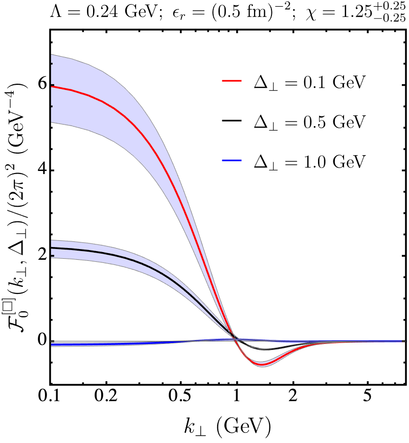
Figure 2: The function ${\cal F}_{0}^{[\Box]}/(2\pi)^{2}$ as a function of the transverse momentum $k_{\perp}$ for three different values of $\Delta_{\perp}$ for the choice $\epsilon_{r}=(0.5\,{\rm fm})^{-2}$. The curves are for $\chi=1.25$ and the bands around them correspond to $\chi$ in the range from 1.0 to 1.5, where larger $\chi$ yields larger results.

IV Exclusive Diffractive dijet production cross sections

The cross section for the diffractive dijet production process $\gamma^{*}p(A)\rightarrow q\bar{q}p(A)$ can be calculated at leading order (LO) by combining two steps: 1) the incoming virtual photon which splits into a quark-antiquark dipole pair and 2) the interaction of the pair with the proton or nucleus via two-gluon exchange. The LO of the virtual photon light cone wave function with virtuality $Q$ is discussed in many papers, such as Beuf:2011xd ; Altinoluk:2015dpi ; Hanninen:2017ddy which we follow to arrive at the cross section expressions:

$$\frac{d\sigma^{\gamma^{*}p}_{T,L}}{dz_{1}dz_{2}d^{2}\bm{K}_{\perp}d^{2}\bm{\Delta}_{\perp}}=\frac{1}{2(2\pi)^{5}z_{1}z_{2}}\delta(z_{1}+z_{2}-1)\sum_{\beta_{i}h_{i}}\left|\left\langle\mathcal{M}_{q\bar{q}}\right\rangle_{C}\right|^{2},$$ (21)

where $\mathcal{M}_{q\bar{q}}$ denotes the amplitude of this process, $z_{1,2}=k_{1,2}^{+}/k^{+}$ are the outgoing quark and antiquark longitudinal momentum fraction w.r.t. the virtual photon longitudinal momentum, and the sum is over color indices $\beta_{i}$ and quark helicities $h_{i}$. For the case of a transverse photon the amplitude is given by:

$$\mathcal{M}^{T}_{q\bar{q}} = ee_{f}\sqrt{z_{1}z_{2}}\left[z_{2}-z_{1}-2h_{0}\lambda\right]\delta_{h_{0},-h_{1}}\ \int d^{2}\bm{q}_{\perp}\int\frac{d^{2}\bm{r}_{\perp}\,d^{2}\bm{b}_{\perp}}{(2\pi)^{2}}e^{-i\bm{b}_{\perp}\cdot\bm{\Delta}_{\perp}}e^{-i\bm{r}_{\perp}\cdot\bm{q}_{\perp}}$$ (22)

$$\times \left[U_{\beta_{0}\beta_{1}}^{[\Box]}(\bm{b}_{\perp}-\frac{\bm{r}_{\perp}}{2},\bm{b}_{\perp}+\frac{\bm{r}_{\perp}}{2})-\delta_{\beta_{0}\beta_{1}}\right]\frac{\bm{\epsilon}_{\lambda}\cdot\left(\bm{K}_{\perp}-\bm{q}_{\perp}\right)}{z_{1}z_{2}Q^{2}+\left(\bm{K}_{\perp}-\bm{q}_{\perp}\right)^{2}},$$

and for a longitudinal photon by:

$$\mathcal{M}^{L}_{q\bar{q}} = -2ee_{f}\sqrt{z_{1}z_{2}}\delta_{h_{0},-h_{1}}\int d^{2}\bm{q}_{\perp}\int\frac{d^{2}\bm{r}_{\perp}\,d^{2}\bm{b}_{\perp}}{(2\pi)^{2}}e^{-i\bm{b}_{\perp}\cdot\bm{\Delta}_{\perp}}e^{-i\bm{r}_{\perp}\cdot\bm{q}_{\perp}}$$ (23)

$$\times \left[U_{\beta_{0}\beta_{1}}^{[\Box]}(\bm{b}_{\perp}-\frac{\bm{r}_{\perp}}{2},\bm{b}_{\perp}+\frac{\bm{r}_{\perp}}{2})-\delta_{\beta_{0}\beta_{1}}\right]\frac{z_{1}z_{2}Q}{z_{1}z_{2}Q^{2}+(\bm{K}_{\perp}-\bm{q}_{\perp})^{2}},$$

where $\bm{\epsilon}_{\lambda}$ denotes the polarization vector of a photon with helicity $\lambda$. After averaging over color and photon polarization, and after summing over quark helicities Altinoluk:2015dpi , we arrive at:

$$\frac{d\sigma^{\gamma^{*}p}_{T}}{dz_{1}dz_{2}d^{2}\bm{K}_{\perp}d^{2}\bm{\Delta}_{\perp}}= \frac{\alpha_{em}}{8(2\pi)^{4}N_{c}}\sum_{f}e_{f}^{2}\ \delta(z_{1}+z_{2}-1)\left[z_{1}^{2}+z_{2}^{2}\right]\int d^{2}\bm{q}_{\perp}\ \int d^{2}\bm{q}_{\perp}^{\prime}\ {\cal F}^{[\Box]}(\bm{q}_{\perp},\bm{\Delta}_{\perp})$$ (24)

$$\times{\cal F}^{[\Box]}(\bm{q}_{\perp}^{\prime},\bm{\Delta}_{\perp})\left[\frac{\left(\bm{K}_{\perp}-\bm{q}_{\perp}\right)}{z_{1}z_{2}Q^{2}+\left(\bm{K}_{\perp}-\bm{q}_{\perp}\right)^{2}}\right]\cdot\left[\frac{\left(\bm{K}_{\perp}-\bm{q}_{\perp}^{\prime}\right)}{z_{1}z_{2}Q^{2}+\left(\bm{K}_{\perp}-\bm{q}_{\perp}^{\prime}\right)^{2}}\right],$$

and

$$\frac{d\sigma^{\gamma^{*}p}_{L}}{dz_{1}dz_{2}d^{2}\bm{K}_{\perp}d^{2}\bm{\Delta}_{\perp}}= \frac{\alpha_{em}}{2(2\pi)^{4}N_{c}}\sum_{f}e_{f}^{2}\ \delta(z_{1}+z_{2}-1)\ z_{1}^{2}z_{2}^{2}Q^{2}\int d^{2}\bm{q}_{\perp}\ \int d^{2}\bm{q}_{\perp}^{\prime}\ {\cal F}^{[\Box]}(\bm{q}_{\perp},\bm{\Delta}_{\perp})$$ (25)

$$\times{\cal F}^{[\Box]}(\bm{q}_{\perp}^{\prime},\bm{\Delta}_{\perp})\frac{1}{z_{1}z_{2}Q^{2}+\left(\bm{K}_{\perp}-\bm{q}_{\perp}\right)^{2}}\frac{1}{z_{1}z_{2}Q^{2}+\left(\bm{K}_{\perp}-\bm{q}_{\perp}^{\prime}\right)^{2}}.$$

As discussed earlier we will only consider the angular independent part ${\cal F}_{0}^{[\Box]}$.

We note that since there is an average over the color configurations of the target, the cross section will scale as $N_{c}$, the sum over colors of the quark-antiquark pair. Since we express the cross section in terms of GTMDs that themselves scale as $N_{c}$, the above expressions have an overall $1/N_{c}$ factor, rather than $N_{c}$ like in e.g. Altinoluk:2015dpi . But the results are consistent with each other.

In order to relate $\sigma^{\gamma^{*}p}$ to the diffractive dijet cross section $\sigma^{ep}$ for electron-proton collisions in DIS in HERA experiments, one can use Altinoluk:2015dpi

$$\frac{d\sigma^{ep}}{dx\ dQ^{2}}=\frac{\alpha_{em}}{\pi xQ^{2}}\left[\left(1-y+\frac{y^{2}}{2}\right)\sigma^{\gamma^{*}p}_{T}+\left(1-y\right)\sigma^{\gamma^{*}p}_{L}\right],$$ (26)

with $y=Q^{2}/sx$ and $\sqrt{s}$ is the center of mass energy of $ep$ collision, which for the H1 data to be discussed was 319 GeV. We will fit the resulting expression to the high $Q^{2}$ electroproduction data of H1 and make predictions for high $Q^{2}$ electroproduction at EIC. We will also make predictions for photoproduction, which we now discuss.

IV.1 Photoproduction: $Q^{2}=0$

For the case of $Q^{2}=0$ the expression for $d\sigma^{\gamma^{*}p}_{T}$ can be used to arrive at:

$$\frac{d\sigma^{\gamma p}}{dz_{1}dz_{2}d^{2}\bm{K}_{\perp}d^{2}\bm{\Delta}_{\perp}}= \frac{\alpha_{em}}{8(2\pi)^{4}N_{c}}\sum_{f}e_{f}^{2}\ \delta(z_{1}+z_{2}-1)\left[z_{1}^{2}+z_{2}^{2}\right]\int d^{2}\bm{q}_{\perp}\ \int d^{2}\bm{q}_{\perp}^{\prime}\ {\cal F}^{[\Box]}(\bm{q}_{\perp},\bm{\Delta}_{\perp})$$ (27)

$$\times{\cal F}^{[\Box]}(\bm{q}_{\perp}^{\prime},\bm{\Delta}_{\perp})\left[\frac{\left(\bm{K}_{\perp}-\bm{q}_{\perp}\right)}{\left(\bm{K}_{\perp}-\bm{q}_{\perp}\right)^{2}}\right]\cdot\left[\frac{\left(\bm{K}_{\perp}-\bm{q}_{\perp}^{\prime}\right)}{\left(\bm{K}_{\perp}-\bm{q}_{\perp}^{\prime}\right)^{2}}\right].$$

The integrations over the angles of $\bm{q}_{\perp}$ and $\bm{q}_{\perp}^{\prime}$ can be calculated analytically to arrive at Hagiwara:2017fye ; Pelicer:2018clw

$$\int d^{2}\bm{q}_{\perp}\frac{{\cal F}_{0}^{[\Box]}(q_{\perp},{\Delta}_{\perp})\left(\bm{K}_{\perp}-\bm{q}_{\perp}\right)}{\left(\bm{K}_{\perp}-\bm{q}_{\perp}\right)^{2}}=\frac{(2\pi)^{3}\bm{K}_{\perp}}{K_{\perp}^{2}}A_{T}(K_{\perp},\Delta_{\perp}),$$ (28)

with

$$A_{T}(K_{\perp},\Delta_{\perp})=\frac{1}{(2\pi)^{2}}\int_{0}^{K_{\perp}}dq_{\perp}\,q_{\perp}\,{\cal F}_{0}^{[\Box]}(q_{\perp},{\Delta}_{\perp}).$$ (29)

In Fig. 3 we show the function $A_{T}(K_{\perp},\Delta_{\perp})$ as a function of $K_{\perp}$ for the same parameters choices and ranges as in Fig. 2. It shows that the function is already very small when $\Delta_{\perp}=1$ GeV.

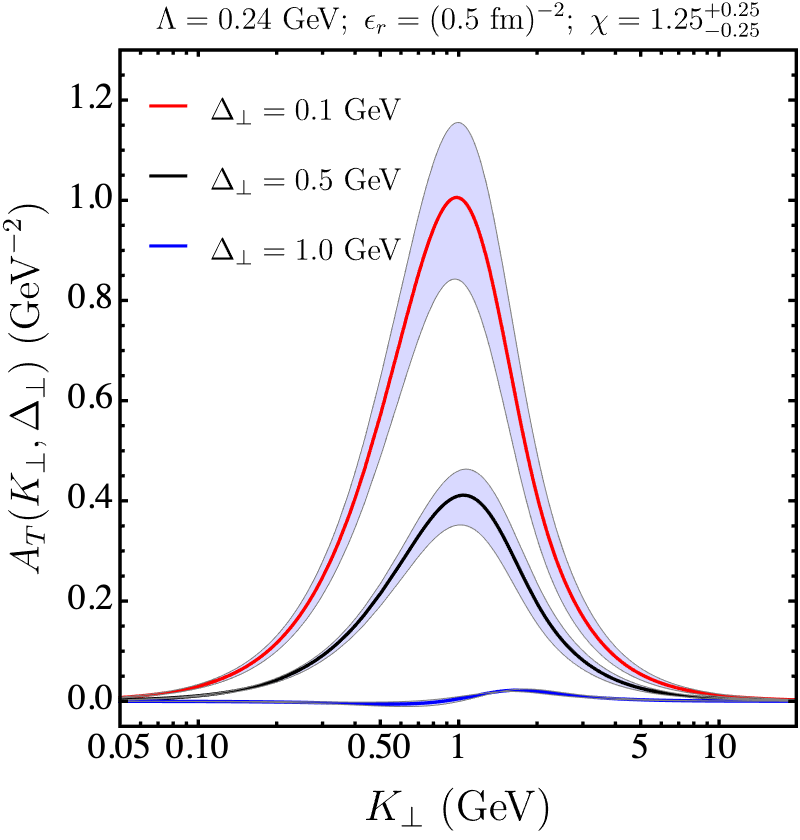
Figure 3: The function $A_{T}(K_{\perp},\Delta_{\perp})$ as a function of $K_{\perp}$ for three different values of $\Delta_{\perp}$.

The $\gamma p$ differential cross section can thus be written as:

$$\frac{d\sigma^{\gamma p}}{dz_{1}dz_{2}dK_{\perp}d\Delta_{\perp}^{2}}= \frac{(2\pi)^{4}\alpha_{em}}{16N_{c}}\sum_{f}e_{f}^{2}\ \delta(z_{1}+z_{2}-1)\left[z_{1}^{2}+z_{2}^{2}\right]\frac{A^{2}_{T}(K_{\perp},\Delta_{\perp})}{K_{\perp}}.$$ (30)

IV.2 Electroproduction: $Q^{2}>0$

For the case of $Q^{2}>0$ the cross section receives contributions from both the transverse and the longitudinal polarization states of the photon. The integrations over the angles of $\bm{q}_{\perp}$ and $\bm{q}_{\perp}^{\prime}$ can again be calculated analytically to arrive for the transverse part in Eq. (24) at

$$\int d^{2}\bm{q}_{\perp}\mathcal{F}^{[\Box]}_{0}(q_{\perp},{\Delta_{\perp}})\left[\frac{\left(\bm{K}_{\perp}-\bm{q}_{\perp}\right)}{z_{1}z_{2}Q^{2}+\left(\bm{K}_{\perp}-\bm{q}_{\perp}\right)^{2}}\right]=\frac{(2\pi)^{3}\bm{K}_{\perp}}{K_{\perp}^{2}}{\cal A}_{\text{T}}(K_{\perp},\Delta_{\perp},z_{i},Q)$$ (31)

with

$${\cal A}_{\text{T}}(K_{\perp},\Delta_{\perp},z_{i},Q)=\frac{1}{(2\pi)^{2}}\int_{0}^{\infty}dq_{\perp}\ \frac{q_{\perp}\ \mathcal{F}^{[\Box]}_{0}(q_{\perp},{\Delta_{\perp}})}{2}\left[1+\frac{K_{\perp}^{2}-q_{\perp}^{2}-z_{1}z_{2}Q^{2}}{\sqrt{(K_{\perp}^{2}+q_{\perp}^{2}+z_{1}z_{2}Q^{2})^{2}-(2K_{\perp}q_{\perp})^{2}}}\right],$$ (32)

while for the longitudinal part in Eq. (25) can be evaluated to be

$$\int d^{2}\bm{q}_{\perp}\mathcal{F}^{[\Box]}_{0}(q_{\perp},{\Delta_{\perp}})\left[\frac{Q}{z_{1}z_{2}Q^{2}+\left(\bm{K}_{\perp}-\bm{q}_{\perp}\right)^{2}}\right]=\frac{(2\pi)^{3}K_{\perp}}{K_{\perp}^{2}}{\cal A}_{\text{L}}(K_{\perp},\Delta_{\perp},z_{i},Q)$$ (33)

with

$${\cal A}_{\text{L}}(K_{\perp},\Delta_{\perp},z_{i},Q)=\frac{1}{(2\pi)^{2}}\int_{0}^{\infty}\ dq_{\perp}\ q_{\perp}\ \mathcal{F}^{[\Box]}_{0}(q_{\perp},{\Delta_{\perp}})\left[\frac{K_{\perp}Q}{\sqrt{(K_{\perp}^{2}+q_{\perp}^{2}+z_{1}z_{2}Q^{2})^{2}-(2K_{\perp}q_{\perp})^{2}}}\right].$$ (34)

Therefore, the $\gamma^{*}p$ differential cross section for $Q^{2}>0$ can be expressed in terms of ${\cal A}_{\text{T}}$ and ${\cal A}_{\text{L}}$ as

$$\frac{d\sigma^{\gamma^{*}p}_{L}}{dz_{1}dz_{2}dK_{\perp}d\Delta_{\perp}^{2}}=\frac{(2\pi)^{4}\alpha_{em}}{16N_{c}}\sum_{f}e_{f}^{2}\ \delta(z_{1}+z_{2}-1)\left[z_{1}^{2}+z_{2}^{2}\right]\frac{{\cal A}^{2}_{\text{T}}(K_{\perp},\Delta_{\perp},z_{i},Q)}{K_{\perp}}$$ (35)

and

$$\frac{d\sigma^{\gamma^{*}p}_{L}}{dz_{1}dz_{2}dK_{\perp}d\Delta_{\perp}^{2}}=\frac{(2\pi)^{4}\alpha_{em}}{4N_{c}}\sum_{f}e_{f}^{2}\ \delta(z_{1}+z_{2}-1)z_{1}^{2}z_{2}^{2}\frac{{\cal A}^{2}_{\text{L}}(K_{\perp},\Delta_{\perp},z_{i},Q)}{K_{\perp}}.$$ (36)

In Figs. 5 and 5 we show the functions ${\cal A}_{\text{T}}$ and ${\cal A}_{\text{L}}$ for the same parameter choices as in Fig. 2 and Fig. 3, and for $Q^{2}=4\ \text{GeV}^{2}$ and $z_{1}=z_{2}=0.5$. It can be seen that the magnitude of ${\cal A}_{\text{L}}$ is larger than ${\cal A}_{\text{T}}$. However, the $z_{1}^{2}z_{2}^{2}$ term in front of ${\cal A}_{\text{L}}$ makes its contribution to the differential cross section much smaller as can be seen in the next section. In Figs. 7 and 7 we show ${\cal A}_{\text{T}}$ and ${\cal A}_{\text{L}}$ for different values of $Q^{2}$.

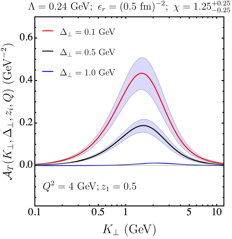
Figure 4: The function ${\cal A}_{\text{T}}$ as a function of $K_{\perp}$ from Eq. (32) for three different values of $\Delta_{\perp}$, $Q^{2}=4\ \text{GeV}^{2}$, and $z_{1}=z_{2}=0.5$.

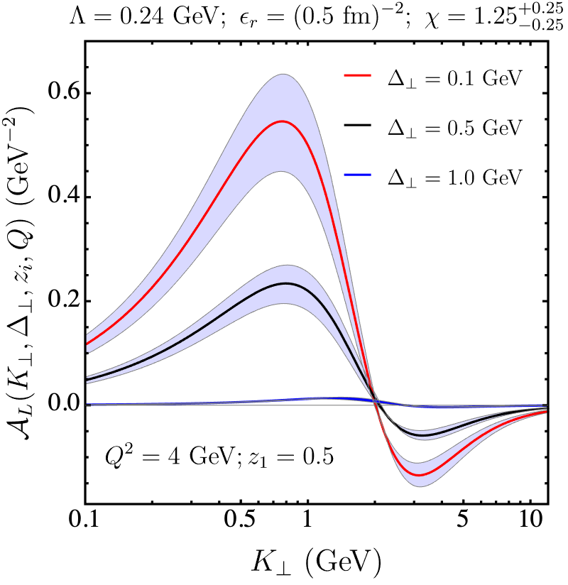
Figure 5: The function ${\cal A}_{\text{L}}$ as a function of $K_{\perp}$ from Eq. (34) for three different values of $\Delta_{\perp}$, $Q^{2}=4\ \text{GeV}^{2}$, and $z_{1}=z_{2}=0.5$.

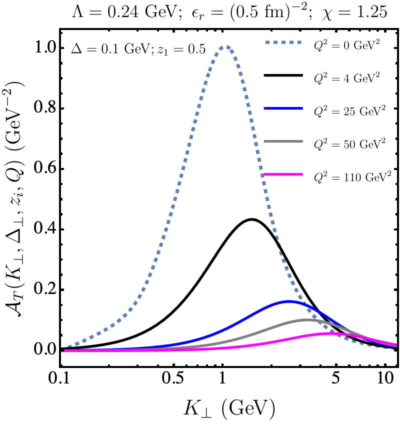
Figure 6: The function ${\cal A}_{\text{T}}$ as a function of $K_{\perp}$ from Eq. (32) for five different values of $Q^{2}$, $\Delta_{\perp}=0.1\ \text{GeV}$, and $z_{1}=z_{2}=0.5$.

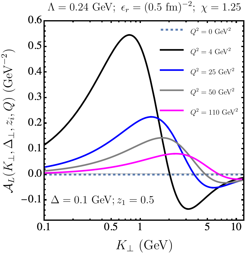
Figure 7: The function ${\cal A}_{\text{L}}$ as a function of $K_{\perp}$ from Eq. (34) for five different values of $Q^{2}$, $\Delta_{\perp}=0.1\ \text{GeV}$, and $z_{1}=z_{2}=0.5$.

V Model fit of H1 data

The H1 and ZEUS experiments at HERA have studied the diffractive dijet process in a series of papers Aktas:2007bv ; Aaron:2011mp ; Abramowicz:2015vnu . Here we focus on Aaron:2011mp where data in the $Q^{2}$ range of $4-110\ {\rm GeV}^{2}$ was presented, for $y\in[0.05,0.7]$ and $|t|\leq 1\ {\rm GeV}^{2}$, that allows us to study the correlation limit region . Given this $Q^{2}$ range we consider the case of four flavors. The H1 cross sections for two central jets shown in Fig. 9 are obtained by extrapolation to the range $|t_{\text{min}}|\leq|t|\leq 1\ \text{GeV}^{2}$ in order to compare to earlier results Aktas:2007bv . We fit our model to this extrapolation range. Here, $|t_{\text{min}}|$ is the minimum kinematically accessible value of $|t|$. In our case $|t|=\Delta_{\perp}^{2}$.

We first consider the data for the $t$-dependence of the differential cross section based on Eqs. (35) and (36). We select $\epsilon_{r}=(0.5\,{\rm fm})^{-2}$ and find that $\chi=1.25$ can describe the data quite well, as shown in Fig. 9, which has a very clear $e^{-bt}$ dependence, with $b\approx 6\ {\rm GeV}^{2}$. The slope of the cross section as a function of $|t|$ is controlled by the proton profile in Eq. (16). The H1 data description does not depend much on $\epsilon_{r}$, therefore, we have chosen $\epsilon_{r}=0.5\ \text{fm}$ in line with the gluonic radius of the proton $R_{p}$.

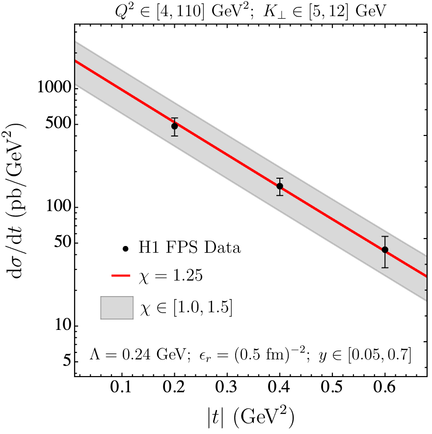
Figure 8: Differential cross section as a function of $|t|$ for the model for the indicated parameter choices and ranges, and for the H1 FPS data including the total uncertainties $\delta_{\text{tot}}$.

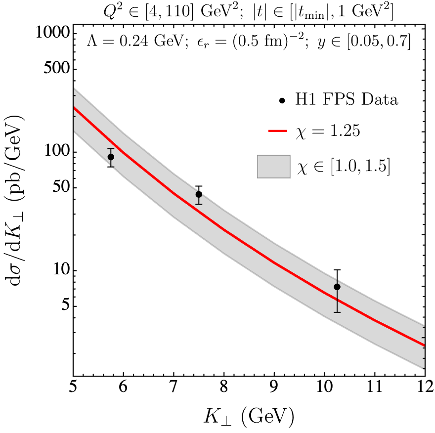
Figure 9: Differential cross section as a function of $K_{\perp}\approx k_{1\perp}$ for the model for the indicated parameter choices and ranges ($t_{\min}\approx 0$), and for the H1 FPS data including the total uncertainties $\delta_{\text{tot}}$.

We also display a band corresponding to $\chi$ in the range from 1.0 to 1.5. This range is selected on the basis of the $K_{\perp}$-dependence of the differential cross section. The H1 data is actually presented as a function of the transverse momentum of one of the jets, which is large (in the range $5-12\ {\rm GeV}$) and almost back-to-back with the other jet in the transverse plane, such that one can expect that $q_{\perp}\ll K_{\perp}$, although the values of $q_{\perp}$ are not included in Aaron:2011mp . On the basis of this expectation we approximate $K_{\perp}=(k_{1\perp}-k_{2\perp})/2=k_{1\perp}-q_{\perp}/2\approx k_{1\perp}$. The result is shown in Fig. 9. As can be seen the transverse momentum dependence does not show as clear a power law fall-off as the model curves, hence, the considerable uncertainty in the $\chi$ value. The contribution of the longitudinal part to the cross section is not very large, it is 12 % at $K_{\perp}=12$ GeV and becomes smaller for smaller $K_{\perp}$, e.g. it is 3.5 % for $K_{\perp}=5$ GeV.

For the description of the H1 data we selected values for $\chi$ in the range $1.0-1.5$ with a central value $\chi=1.25$. One could relate these values using the GBW model expression for the saturation scale to corresponding $x$ values: $\chi=2(3\cdot 10^{-4}/x)^{0.3}$, such that $\chi=1.25\pm 0.25$ corresponds to $x\sim(1-3)\cdot 10^{-3}$. We consider such $\chi$ values to be acceptable and consistent with the typical $x$ values at which the MV model is generally considered to be applicable. Selecting a fixed $\chi$ value corresponds to selecting an average $x$ value. In Fig. 10 we show the $Q^{2}$ dependence of the model in comparison to the H1 data. It shows that for smaller $Q^{2}$, which corresponds to smaller $x$ values for given $y$ and $s$, a larger $\chi$ value is needed, whereas at larger $Q^{2}$, a smaller $\chi$ value is needed. Clearly a better description of the $Q^{2}$ dependence of the data could be obtained with an $x$-dependent $\chi$. However, since the integral of a curve through the central values of the H1 data as function of $Q^{2}$ is found to fall within the range of the $Q^{2}$ integral of the model, we proceed with the model with a fixed $\chi$, i.e. with an average $x$. We note that the H1 data spans an $x$ range from $5\cdot 10^{-5}$ to 0.02, giving a geometric mean of $10^{-3}$, which corresponds well with the $x$ values we obtain from the GBW model expression for the $\chi$ values considered.

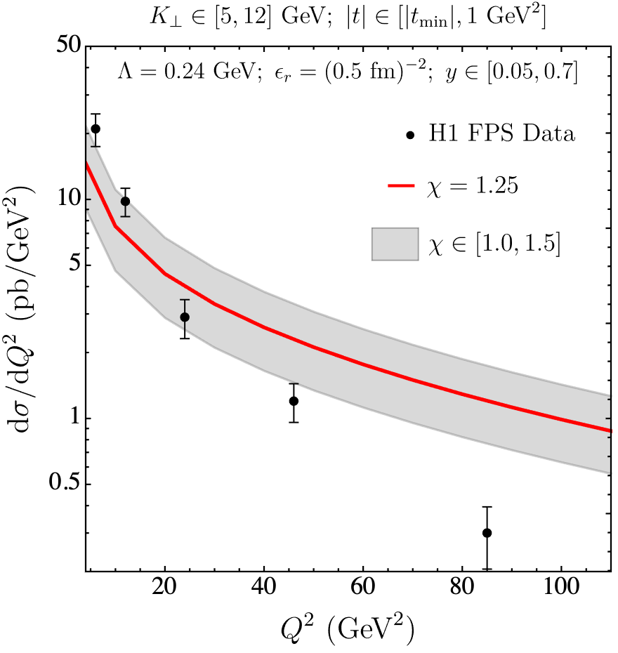
Figure 10: Differential cross section as a function of $Q^{2}$ for the model for the indicated parameter choices and ranges ($t_{\min}\approx 0$), and for the H1 FPS data including the total uncertainties $\delta_{\text{tot}}$.

All in all, we conclude that the GTMD model allows for a fair description of the diffractive dijet production H1 data, for reasonable model parameters, in reasonable agreement with assumptions on the gluonic radius and the $x$ values the model applies to.

VI Model predictions for EIC

In this final section we present predictions for exclusive diffractive dijet production at the EIC using our model. For leptoproduction we consider the range $3\leq K_{\perp}\leq 9\ {\rm GeV}$, because the center of mass energy of EIC will be lower than at HERA. At even lower $K_{\perp}$ we expect that jets cannot be resolved anymore and by selecting this range, we can consider the fixed flavor case with $N_{f}=4$. We consider $Q^{2}\in[1\ {\rm GeV}^{2},K_{\perp}^{2}]$ rather than the fixed range $Q^{2}\in[4,110]\ {\rm GeV}^{2}$ of HERA and also show the cases for $Q^{2}=K_{\perp}^{2}$ and $Q^{2}=4K_{\perp}^{2}$ (here we expect smaller $Q^{2}$ to be better described by larger $\chi$ and vice versa). We also present model predictions for photoproduction. As expected, the cross section is much larger in this case.

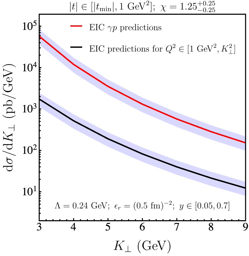
Figure 11: Predictions for exclusive diffractive dijet production in $ep$ (black curve) and $\gamma p$ (red curve) collisions at the EIC.

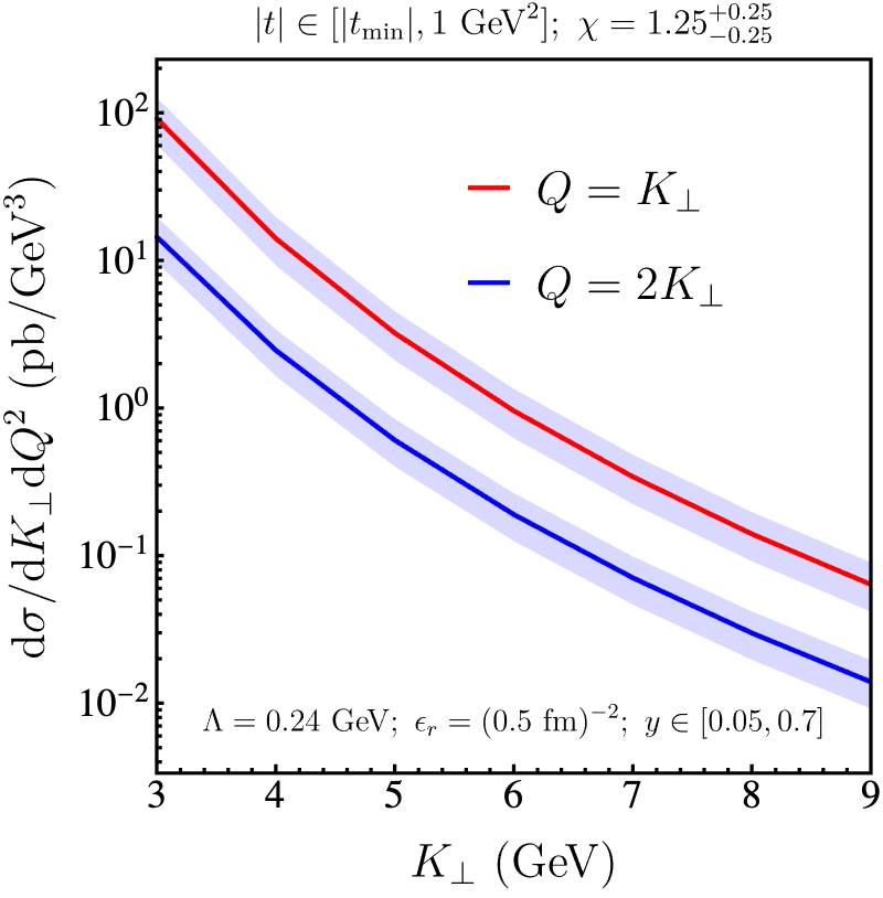
Figure 12: Predictions for exclusive diffractive dijet production in $ep$ collisions at the EIC for $Q=K_{\perp}$ and $Q=2K_{\perp}$.

The photoproduction result can also be translated into predictions for Ultra-Peripheral Collisions (UPCs) in p-Pb and Pb-Pb collisions at the LHC upon folding in the appropriate photon distribution inside a Pb nucleus, cf. Hagiwara:2017fye . However, if in such collisions $K_{\perp}$ values are reached that are much larger than $Q_{s}$, then the saturation description may no longer be appropriate. Also it is important that the dijet pair has a rapidity gap in order to ensure a diffractive process. The only currently available UPC jet production data is by the ATLAS collaboration Angerami:2017kot , where such a rapidity gap condition is not imposed however. The diffractive contribution was estimated to be at most at the 5% level for the small $x$ part of the data Guzey:2020ehb and it may thus not be surprising that our GTMD model cannot describe those ATLAS UPC data, underestimating the cross section by two or three orders of magnitude. In contrast, the collinear factorization description of Guzey:2018dlm at NLO is able to describe the ATLAS data well. Predictions for UPCs in a kinematic regime appropriate for our GTMD model will be considered elsewhere.

VII Conclusions

We have considered a small-$x$ model for gluon GTMDs that is based on the MV model with an impact parameter dependent saturation scale, introducing a few free parameters in order to obtain a good fit to the H1 data on diffractive dijet production in electron-proton collisions. The values of the free parameters turn out to be reasonable from the physical interpretation point of view. With this we obtain a good description of the $|t|$ dependence of the data and a reasonable description of the jet transverse momentum dependence. This provides confidence that the gluon GTMD description is appropriate for this process in the examined kinematic range. With this model we provide predictions for the EIC for both electroproduction in a somewhat different kinematic regime and for photoproduction which has a much higher cross section. We hope that this will allow further tests of the underlying GTMD description.

We also have addressed some theoretical issues known from GPD and small $x$ studies that are relevant for small-$x$ gluon GTMD models with an impact parameter dependent saturation scale. First there is the issue that considering the impact parameter dependence requires the target (and the dipole) to be sufficiently localized in transverse coordinate space. This in turn requires consideration of the dipole frame with large $P^{+}$ and hence sufficiently large center of mass energy. Second, the dipole size has to be much smaller than the size of the impact parameter profile considered. This requires consideration of the correlation limit for dijet production, in which $\Delta_{\perp}=k_{1\perp}+k_{2\perp}$ is much smaller than $K_{\perp}=(k_{1\perp}-k_{2\perp})/2\approx k_{1\perp}\approx k_{2\perp}$, where the latter scale determines the relevant dipole sizes. On the other hand, $K_{\perp}$ should not be so large that one is outside the saturation regime. Under these kinematic conditions the MV model with impact parameter dependent saturation scale is expected to be an appropriate model for the gluon GTMDs probed. The fairly good description of the H1 data gives support to this GTMD picture and we hope it can be scrutinized further with future data from EIC and LHC.

References

(1)
X. d. Ji,
Phys. Rev. Lett. 91 (2003) 062001.
(2)
A. V. Belitsky, X. d. Ji and F. Yuan,
Phys. Rev. D 69 (2004) 074014.
(3)
S. Meissner, A. Metz, M. Schlegel and K. Goeke,
JHEP 08 (2008) 038.
(4)
S. Meissner, A. Metz and M. Schlegel,
JHEP 08 (2009) 056.
(5)
C. Lorcé, B. Pasquini and M. Vanderhaeghen,
JHEP 05 (2011) 041.
(6)
M. G. Echevarria et al., Phys. Lett. B 759 (2016) 336-341.
(7)
J. More, A. Mukherjee and S. Nair,
Eur. Phys. J. C 78 (2018) no.5, 389.
(8)
Y. Hatta, B. W. Xiao and F. Yuan,
Phys. Rev. Lett. 116 (2016) no.20, 202301.
(9)
V. M. Braun and D. Y. Ivanov,
Phys. Rev. D 72 (2005) 034016.
(10)
T. Altinoluk, N. Armesto, G. Beuf and A. H. Rezaeian,
Phys. Lett. B 758 (2016) 373-383.
(11)
G. M. Peccini, L. S. Moriggi and M. V. T. Machado,
Phys. Rev. C 102 (2020) no.3, 034903.
(12)
N. Kaur and H. Dahiya,
Eur. Phys. J. A 56 (2020) no.6, 172.
(13)
X. Luo and H. Sun,
Eur. Phys. J. C 80 (2020) no.9, 828.
(14)
J. L. Zhang, Z. F. Cui, J. Ping and C. D. Roberts,
Eur. Phys. J. C 81 (2021) no.1, 6.
(15)
L. D. McLerran and R. Venugopalan,
Phys. Rev. D 49 (1994) 2233.
(16)
L. D. McLerran and R. Venugopalan,
Phys. Rev. D 49 (1994) 3352.
(17)
L. D. McLerran and R. Venugopalan,
Phys. Rev. D 50 (1994) 2225.
(18)
J. Zhou,
Phys. Rev. D 94 (2016) no.11, 114017.
(19)
Y. Hagiwara, Y. Hatta and T. Ueda,
Phys. Rev. D 94 (2016) no.9, 094036.
(20)
Y. Hagiwara, Y. Hatta, R. Pasechnik, M. Tasevsky and O. Teryaev,
Phys. Rev. D 96 (2017) no.3, 034009.
(21)
H. Mäntysaari, N. Mueller and B. Schenke,
Phys. Rev. D 99 (2019) no.7, 074004.
(22)
F. Salazar and B. Schenke,
Phys. Rev. D 100 (2019) no.3, 034007.
(23)
Y. Hatta, B. W. Xiao, F. Yuan and J. Zhou,
Phys. Rev. Lett. 126 (2021) no.14, 142001.
(24)
[CMS Collab.],
“Angular correlations in exclusive dijet photoproduction in ultra-peripheral PbPb collisions at ,”
CMS Physics Analysis Summary, CMS-PAS-HIN-18-011.
(25)
D. E. Soper,
Phys. Rev. D 15 (1977) 1141.
(26)
M. Diehl,
Eur. Phys. J. C 25 (2002) 223-232
[erratum: Eur. Phys. J. C 31 (2003) 277-278].
(27)
M. Burkardt,
Phys. Rev. D 66 (2002) 114005.
(28)
M. Burkardt,
Phys. Rev. D 62 (2000) 071503
[erratum: Phys. Rev. D 66 (2002) 119903].
(29)
M. Burkardt,
Int. J. Mod. Phys. A 18 (2003) 173-208.
(30)
G. A. Miller,
Phys. Rev. C 99 (2019) no.3, 035202.
(31)
R. L. Jaffe,
Phys. Rev. D 103 (2021) no.1, 016017.
(32)
D. Boer,
AIP Conf. Proc. 768 (2005) no.1, 248-252.
(33)
D. Boer, T. Van Daal, P. J. Mulders and E. Petreska,
JHEP 07 (2018) 140.
(34)
A. H. Mueller, “Parton saturation: An Overview,”
[arXiv:hep-ph/0111244 [hep-ph]].
(35)
J. Bartels, K. J. Golec-Biernat and K. Peters,
Acta Phys. Polon. B 34 (2003) 3051-3068.
(36)
F. Gelis, E. Iancu, J. Jalilian-Marian, and R. Venugopalan, Ann. Rev. Nucl. Part. Sci. 60 (2010) 463.
(37)
F. Gelis and A. Peshier,
Nucl. Phys. A 697 (2002) 879-901.
(38)
A. H. Mueller,
Nucl. Phys. B 335 (1990) 115-137.
(39)
K. J. Golec-Biernat and A. M. Stasto,
Nucl. Phys. B 668 (2003) 345-363.
(40)
E. Iancu and A. H. Rezaeian,
Phys. Rev. D 95 (2017) no.9, 094003.
(41)
K. J. Golec-Biernat and M. Wüsthoff,
Phys. Rev. D 59 (1998) 014017.
(42)
G. Beuf,
Phys. Rev. D 85 (2012) 034039.
(43)
H. Hänninen, T. Lappi and R. Paatelainen,
Annals Phys. 393 (2018) 358-412.
(44)
M. Reinke Pelicer, E. Gräve De Oliveira and R. Pasechnik,
Phys. Rev. D 99 (2019) no.3, 034016.
(45)
A. Aktas et al. [H1 Collab.],
JHEP 10 (2007) 042.
(46)
F. D. Aaron et al. [H1 Collab.],
Eur. Phys. J. C 72 (2012) 1970.
(47)
H. Abramowicz et al. [ZEUS Collab.],
Eur. Phys. J. C 76 (2016) no.1, 16.
(48)
R. Boussarie, A. V. Grabovsky, L. Szymanowski and S. Wallon,
Phys. Rev. D 100 (2019) no.7, 074020.
(49)
A. Angerami [ATLAS],
Nucl. Phys. A 967 (2017) 277-280.
(50)
V. Guzey and M. Klasen,
[arXiv:2012.13277 [hep-ph]].
(51)
V. Guzey and M. Klasen,
Phys. Rev. C 99 (2019) no.6, 065202.