Benchmark computations for the polarization tensor characterization of small conducting objects

Abstract

The characterisation of small low conducting inclusions in an otherwise uniform background from low-frequency electrical field measurements has important applications in medical imaging using electrical impedance tomography as well as in geological imaging using electrical resistivity tomography. It is known that such objects can be characterised by a Póyla-Szegö (polarizability) tensor. Such characterisations have attracted interest as they can provide object features in a machine learning classification algorithm and provide an alternative imaging solution. However, to be able train machine learning algorithms, large dictionaries are required and it is essential that the characterisations are accurate. In this work, we obtain accurate numerical approximations to the tensor coefficients, by applying an adaptive boundary element method. The goal being to provide a sequence of benchmark computations for the tensor coefficients to allow other software developers check the accuracy of their codes.

1 Introduction

The purpose of this paper is provide a series of accurate benchmark computations for the Póyla-Szegö tensor (PST) characterisation of small conducting objects with low contrasts. Our benchmark computations are intended to be useful for developers of computational tools for solving partial differential equations and, in particular, for those developing tools that will form part of a machine learning (ML) classification algorithm for detecting and classifying small conducting inclusions.

The characterisation of conducting objects with low conductivities in an otherwise uniform background using low frequency electric fields has a wide range of important applications including medical imaging and geology using electrical impedance tomography (EIT) and electrical resistivity tomography, respectively e.g. [1]. In particular, being able to characterise small objects is important for the related inverse problem where the task is to be able to determine the shape and material contrasts of hidden conducting inclusions from measurements of the induced voltage at the boundary from induced current distributions [2]. This inverse problem was first studied by Calderón [3]. There is a large and increasing literature on the EIT inverse problem and many different computational approaches have been proposed. Some examples of alternative solution approaches include total variational regularisation [4], topological derivative [5] and machine learning approaches [6].

For EIT it has been rigorously proven by Cedio-Fengya, Moskow and Vogelius [7] that an asymptotic expansions of the perturbed field for small objects simply connected in the form $B_{\alpha}:=\alpha B+{\bm{z}}$, where $\alpha$ denotes the object size, $B$ a unit sized object placed at the origin and ${\bm{z}}$ is the translation, in a bounded domain has a leading order term,

$$(u_{\alpha}-u_{0})(\bm{x})= \nabla_{\bm{x}}G(\bm{x},\bm{z})\cdot[{\mathcal{T}}(k,\alpha B)\nabla_{\bm{z}}u_{0}(\bm{z})]+O(\alpha^{4})$$ (1)

as $\alpha\to 0$ where $u_{\alpha}$ denotes the field in the presence of the object, $u_{0}$ denotes the background field, $G(\bm{x},\bm{z}):=1/{(4\pi|\bm{x}-\bm{z}|)}$ is the free space Laplace Green’s function, $k$ denotes the (conductivity) contrast, ${\mathcal{T}}(k,\alpha B)=\sum_{i,j=1}^{3}{\mathcal{T}}_{ij}{\bm{e}}_{i}\otimes{\bm{e}}_{j}$ is the appropriate polarizability tensor (also sometimes known as a polarization tensor) for this problem and ${\bm{e}}_{i}$ the orthonormal coordinate directions. The appropriate polarization tensor for this problem coincides with the PST, which is independent of the object’s position. Ammari and Kang [8, Section 4.1] have derived the corresponding complete asymptotic expansion of this problem and have introduced the concept of generalised polarization tensors, which offer improved object characterisations and have the PST as the simplest type. The same PST object description is also known to characterise scatterers in electromagnetic scattering [9] and it has been proposed that electro-sensing fish use them for sensing their pray [10]. A closely related polarization tensor also describes conducting objects in metal detection [11].

In the majority of EIT approaches, the hidden object’s position and its shape is inferred by finding information about the conductivity distribution in the imaging region. However, an alternative approach is offered by combining dictionaries of object characterisations using PSTs with classification techniques, such as those in ML algorithms (see [12] for a discussion of different approaches), due to the separation of object characterisation and in position in (1). A ML approach to object classification using polarizability tensors has already been shown to be effective for metal detection [13], but for such an approach to be effective for EIT problems, a description of accurate PST coefficients is required.

In this paper, we provide novel computational benchmark computational solutions to a series of PST object characterisations. The non-dimensional benchmark geometries considered are a unit radius sphere, an ellipsoid with principal semi axes $a=1$, $b=0.7$ and $c=0.5$, an L-shape domain $B_{1}\bigcup B_{2}$ with $B_{1}=[0.0,7.8]\times[0.0,2.0]\times[0.0,1.5]$, $B_{2}=[0.0,2.2]\times[2.0,5.6]\times[0.0,1.5]$, the cube $[-1,1]^{3}$, the tetrahedron with vertices

$${\mbox{\boldmath$v$}}_{1}=\begin{pmatrix}0\\ 0\\ 0\end{pmatrix},\ {\mbox{\boldmath$v$}}_{2}=\begin{pmatrix}7\\ 0\\ 0\end{pmatrix},\ {\mbox{\boldmath$v$}}_{3}=\begin{pmatrix}5.5\\ 4.6\\ 0.0\end{pmatrix},\ {\mbox{\boldmath$v$}}_{4}=\begin{pmatrix}3.3\\ 2.0\\ 5.0\end{pmatrix},$$

and the key contained in the rectangular region $B_{3}\bigcup B_{4}\bigcup B_{5}$ where

$$B_{3} =[-7.0,7.0]\times[3.0,15.0]\times[-1.25,1.25],$$

$$B_{4} =[-4.0,4.0]\times{[0.0,3.0]}\times[-1.25,1.25],$$

$$B_{5} =[-3.25,3.25]\times[-19.0,0.0]\times[-1.25,1.25].$$

Each object geometry is centered at the origin and they are scaled by different length scales $\alpha$ in meters. The benchmark computations for the PST coefficients are obtained by post processing the approximate solutions to a transmission problem, which is governed by Laplace’s equation set on an unbounded region surrounding the (scaled) object of interest. Our benchmark computations are not only of interest to EIT practitioners, but are also of interest to other computational partial differential equation solver developers since the PST coefficients can be obtained by a simple post-processing of transmission problem solutions and, by comparing solutions, can provide a measure of accuracy of a given scheme. To ensure our solutions are accurate, and inspired by a previous boundary integral computation of PST coefficients [14], the transmission problem will be solved using a boundary integral approach using the boundary element python package (Bempp, formally known as the BEM++ library) [15], leading to approximate tensor coefficients for different objects. An adaptive boundary integral scheme, which has already been shown to be effective for a capacitive problem [16], is novelly applied to the computation of the PST to generate a set of accurate benchmark computations for different geometries.

The work proceeds as follows: In Section 2, the mathematical model and boundary integral/layer potential formulae to compute the PST are introduced. Then, in Section 3, a brief description of how Bempp can be applied to compute the PST is presented and, in Section 4, the application of an existing adaptive algorithm to the computation of the PST is described. Section 5 describes the geometries used for our benchmark computations and presents numerical results for the accurate computation of the PST using the adaptive algorithm. The paper ends with some concluding remarks in Section 6.

2 Small Object Characterisation

2.1 Model Problem

We following the formulation in Cedio-Fengya, Moskow and Vogelius [7] and Ammari and Kang [8, Section 4.1] restricted to the characterisation of a single Lipschitz bounded simply connected region $B_{\alpha}$ in $\Omega\subset{\mathbb{R}}^{3}$. We let $0<k\neq 1<+\infty$ be the conductivity (contrast) of $B$ to the background (i.e $k=\gamma|_{B_{\alpha}}/\gamma|_{\Omega\setminus B_{\alpha}}$ where $\gamma$ is the electrical conductivity). We set $B_{\alpha}:=\alpha B+{\bm{z}}$, where $\alpha\ll 1$ denotes the (small) object size parameter, $B$ a unit sized object placed at the origin, and ${\bm{z}}$ is the translation, as illustrated in Figure 1. The voltage $U$ in absence of the inclusion is given by the solution to

$$\nabla^{2}U =0 \Omega$$ in

$$\frac{\partial U}{\partial{\mbox{\boldmath$n$}}} =\psi \partial\Omega$$ on

where $\psi$ denotes the imposed current such that $\int_{\partial\Omega}\psi\mathrm{d}{\mbox{\boldmath$x$}}=0$ and $n$ is the unit outward normal to $\partial\Omega$. In the presence of the inclusion, the voltage $u_{\alpha}$ is given by the solution to

$$\nabla\cdot((1+(k-1)\chi(B))\nabla u_{\alpha}) =0 \Omega$$ in

$$\frac{\partial u_{\alpha}}{\partial{\mbox{\boldmath$n$}}} =\psi \partial\Omega$$ on

For this problem, Cedio-Fengya et al prove an asymptotic expansion of the form stated in (1) where the real symmetric rank 2 PST ${\mathcal{T}}:={\mathcal{T}}(k,\alpha B)$ is a function of $k$, $\alpha$, and $B$, but it is independent of $z$. Ammari and Kang obtained similar asymptotic expansions for other closely related problems in EIT. Both Cedio-Fengya et al and Ammari and Kang discuss the extension to multiple inclusions in EIT. Properties of the tensor ${\mathcal{T}}$ are discussed by Cedio-Fengya et al and Ammari and Kang, which we will draw on below. Ammari and Kang also discuss algorithms for recovering PST coefficients from field measurements.

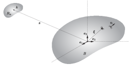
Figure 1: Illustration of physical object $B_{\alpha}$ described as $B_{\alpha}=\alpha B+{\bm{z}}$.

Our interest in this work focus on computational schemes for accurately computing the coefficients of the real symmetric rank 2 PST ${\mathcal{T}}$ for known $\alpha$, $B$, and $k$. We start by recalling a series of alternative, but equivalent formulations of ${\mathcal{T}}$.

2.2 Transmission Problem Formulation

Given the solutions $\vartheta_{i}$, $i=1,2,3$, to the transmission problem

$$\nabla^{2}\vartheta_{i} =0 \hbox{in $B\bigcup B^{c}$},$$ (2a)

$$\left[\vartheta_{i}\right]_{\Gamma} =0 \hbox{on $\Gamma$},$$ (2b)

$${\mbox{\boldmath$n$}}\cdot\nabla\vartheta_{i}\Big{|}_{+}-{\mbox{\boldmath$n$}}\cdot k\nabla\vartheta_{i}\Big{|}_{-} ={\mbox{\boldmath$n$}}\cdot\nabla_{\bm{\xi}}\xi_{i} \hbox{on $\Gamma$},$$ (2c)

$$\vartheta_{i} \to 0 \hbox{as $|\bm{\xi}|\to\infty$},$$ (2d)

where $B^{c}:=\mathbb{R}^{3}\setminus\overline{B}$, $\Gamma:=\partial B$, $\left[\cdot\right]_{\Gamma}=\cdot|_{+}-\cdot|_{-}$ denotes the jump, $\big{|}_{-}$ the interior trace and $\big{|}_{+}$ the exterior trace, $\xi_{j}={\bm{e}}_{j}\cdot{\bm{\xi}}$ denotes the $j$-th the component of ${\bm{\xi}}$ measured from an origin in $B$ and differentiation is with respect to ${\bm{\xi}}$, the coefficients of the PST

$${\mathcal{T}}_{ij}:=\alpha^{3}\left(\left(k-1\right)|B|\delta_{ij}+\left(k-1\right)^{2}\int_{\Gamma}{\mbox{\boldmath$n$}}\cdot\nabla\vartheta_{i}\Big{|}_{-}\xi_{j}\,\mathrm{d}\bm{\xi}\right),$$ (3)

follow by simplifying the result for the coefficients of a GPT in [8, equation (4.10)]. In the above, $|B|$ is the volume of the object and $\delta_{ij}$ is the Kronecker delta. By integration by parts, (3) can be shown to be equivalent to

$${\mathcal{T}}_{ij}:= \alpha^{3}\left(\left(k-1\right)|B|\delta_{ij}-\left(k-1\right)^{2}\left[\int_{B^{c}}\nabla\vartheta_{i}\cdot\nabla\vartheta_{j}\mathrm{d}{\bm{\xi}}\right.\right.$$

$$\left.\left.+\int_{B}k\nabla\vartheta_{i}\cdot\nabla\vartheta_{j}\mathrm{d}{\bm{\xi}}\right]\right),$$

which makes the symmetry of the PST clear. Its independence of ${\bm{z}}$ can similarly be established [7].

2.3 Boundary Integral (BI) Formulation

By following [7, equations (56)-(58)] it is possible to rewrite (3), as follows

$${\mathcal{T}}_{ij}=\alpha^{3}\left(\dfrac{1}{r}|B|\delta_{ij}+\left(1-\dfrac{1}{r}\right)\int_{\Gamma}\psi_{i}n_{j}\,\mathrm{d}\bm{\xi}\right),$$ (4)

where $r=\dfrac{1}{k}$ and $\psi_{i}:=-k\vartheta_{i}$ can be expressed as the solution to the boundary integral equation [7]

$$\psi_{i}(\bm{\xi}):=\frac{1}{r-1}\mathcal{S}\left[\left(\lambda I+\mathcal{K}^{\ast}\right)^{-1}\left({\mbox{\boldmath$n$}}_{\bm{\nu}}\cdot\nabla_{\bm{\nu}}\nu_{i}\right)\right](\bm{\xi}),\quad\forall\bm{\xi}\in\mathbb{R}^{3}.$$ (5)

Here, $\mathcal{S}$ is the single layer potential operator [8, equation (2.12)],

$$\mathcal{S}[f]({\mbox{\boldmath$\xi$}}):=\frac{1}{4\pi}\int_{\Gamma}\frac{1}{|\bm{\xi}-\bm{\nu}|}f({\mbox{\boldmath$\nu$}})\,\mathrm{d}{\mbox{\boldmath$\nu$}},$$

$4\pi$ is the area of the unit sphere in $\mathbb{R}^{3}$, $I$ is the identity operator and $\mathcal{K}^{*}$ is the adjoint double layer boundary operator [8, equation (2.20)],

$$\mathcal{K}^{\ast}[f](\bm{\xi}):=\frac{1}{4\pi}\mbox{ p.v.}\int_{\Gamma}\frac{(\bm{\xi}-\bm{\nu})\cdot{\mbox{\boldmath$n$}}_{\bm{\xi}}}{|\bm{\xi}-\bm{\nu}|^{3}}f(\bm{\nu})\,\mathrm{d}\bm{\nu}.$$

In addition, p.v. denotes the Cauchy principal value, and $|\bm{\xi}-\bm{\nu}|$ is the distance between $\bm{\xi}$ and $\bm{\nu}$, for further details see [8, page 18].

2.4 Layer Potential (LP) Formulation

In [8, Section 4.1], the coefficients of ${\mathcal{T}}$ are shown to be equivalently obtained as follows

$${\mathcal{T}}_{ij}=\alpha^{3}\int_{\Gamma}\xi_{j}\phi_{i}\,\mathrm{d}\bm{\xi},$$ (6)

where $\phi_{i}$ is the solution to the boundary integral equation

$$\phi_{i}(\bm{\xi}):=\left(\lambda I+\mathcal{K}^{*}\right)^{-1}\left({\mbox{\boldmath$n$}}_{\bm{\nu}}\cdot\nabla_{\bm{\nu}}\nu_{i}\right)(\bm{\xi}),\quad\bm{\xi}\in\Gamma,$$ (7)

and $\lambda:=\dfrac{k+1}{2(k-1)}$. Note that, for exact computations, we have $\psi_{i}(\bm{\xi})=\dfrac{1}{r-1}\mathcal{S}\left[\phi_{i}\right]({\bm{\xi}})$.

2.5 Weighted (Alternative) Formulation

By taking a weighted average of (4) and (6) we get

$${\mathcal{T}}_{ij}=\alpha^{3}\left(\dfrac{\beta}{r}|B|\delta_{ij}+\int_{\Gamma}\left(\beta\left(1-\dfrac{1}{r}\right)\psi_{j}n_{i}+\left(1-\beta\right)\phi_{j}\xi_{i}\right)\,\mathrm{d}{\mbox{\boldmath$\xi$}}\right),$$ (8)

with $0\leq\beta\leq 1$. Note that, for $\beta=0$ we obtain the formula (6), whereas for $\beta=1$ we have (4).

3 Computation of the Pólya-Szegö Tensor Coefficients

In this work, we use Bempp [15] to compute the coefficients of the PST. Bempp is a C++ library with Python bindings for the solution of boundary integral equations using Galerkin discretisations described in [15] and further improved in [17]. Note that corners, in contrast to collocation, are not an issue for Galerkin boundary element methods on piecewise smooth Lipschitz domains. We are using fully numerical Erichsen/Sauter type singular quadrature rules that are well suited for this type of discretisation [18]. Given the similarity of the transmission problem (2) and the boundary integral solution formulations (5) and (7) to the capacitive problem already successfully considered in [16], we will focus on a dual mesh discretisation although a primal discretisation is also possible and may also offer further efficiencies. In practice, given a surface mesh discretisation of $B$ of size $h$ we solve for $\phi_{i}^{h}$ and obtain $\psi_{i}^{h}({\bm{\xi}})=\dfrac{1}{r-1}\mathcal{S}\left[\phi_{i}^{h}\right]({\bm{\xi}})$. Following the numerical solution, the discrete approximation ${\mathcal{T}}_{ij}^{h}$ to ${\mathcal{T}}_{ij}$ then follows from a simple postprocessing of the solutions using (8).

Although the coefficients of the true tensor ${\mathcal{T}}$ are symmetric, the coefficients of its numerical approximation ${\mathcal{T}}^{h}$ using boundary elements are not guaranteed to have this property, but tend to a symmetric tensor as the mesh is refined. Thus, to ensure the symmetry of the computed PST, we will symmetrise it as follows:

$${\mathcal{T}}^{h,sym}_{ij}:=\dfrac{1}{2}\left({\mathcal{T}}^{h}_{ij}+{\mathcal{T}}^{h}_{ji}\right).$$

Henceforth, when presenting results, we will only consider the symmetrised tensor and drop the superscript $sym$. In the next section, we illustrate the convergence behaviour of the numerical scheme for uniform grid refinement for a PST with smooth analytical solution.

3.1 Numerical Convergence Study for Ellipsoidal Objects

The convergence of the approximate tensor $\mathcal{T}^{h}$ to the true PST $\mathcal{T}$ obtained on a sequence of uniformly meshes for ellipsoidal objects is investigated. In these experiments, we choose $B_{\alpha}=\alpha B$ and define $B$ by

$$\dfrac{\xi_{1}^{2}}{a^{2}}+\dfrac{\xi_{2}^{2}}{b^{2}}+\dfrac{\xi_{3}^{2}}{c^{2}}=1,\quad 0<c\leq b\leq a.$$

We choose $\alpha=0.01\,\mathrm{m}$ and $k=10$ and consider the cases $a=b=c=1$ so that $B$ degenerates to a sphere and consider the ellipsoid defined by $a=1$, $b=0.7$, $c=0.5$. In Figures 2(a) and  2(b) we show the behaviour of $\|\mathcal{T}^{Exact}-\mathcal{T}^{h}\|/\|\mathcal{T}^{Exact}\|$ with uniform mesh refinement against $1/h$ for different values of $0\leq\beta\leq 1$ and both primal and dual mesh discretisations for both a sphere and an ellipsoid, respectively. Here, $\|\mathcal{T}^{Exact}\|=\left(\sum_{i,j=1}^{3}({\mathcal{T}}_{ij}^{Exact)})^{2}\right)^{1/2}$ is the Frobenius norm and ${\mathcal{T}}^{Exact}$ is the exact solution for these objects [8, page 83]. Specifically, in Figure 2(a), the primal mesh is initially chosen as surface mesh of $232$ surface triangles and then uniformly refined $6$ times until a mesh of $31\,616$ surface triangles is obtained. While in Figure 2(b), the primal mesh is initially chosen as surface mesh of $48$ surface triangles and then uniformly refined $7$ times until a mesh of $65\,566$ surface triangles is obtained. The corresponding dual meshes are obtained from the primal meshes using the procedure described in [16]. Except for a couple of exceptions (eg $\beta=0.4$ shown in Figure 2(a) for the dual mesh), the convergence behaviour for both primal and dual meshes is similar and practically identical for different values of $\beta$. We attribute the exceptions to some super-convergence behaviour in exceptional cases. The fixed convergence rate of the PST under uniform mesh refinement is not surprising given the results of A, which establishes that the convergence behaviour of the coefficients of the PST is the same as the convergence of the solutions to the transmission problem under uniform mesh refinement.

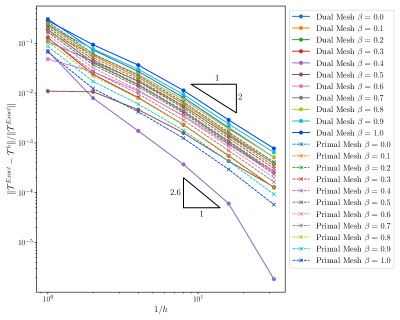
(a) Sphere

(b) Ellipsoid

Figure 2: Relative error between the study of the polarization tensor ${\mathcal{T}}^{h}$ (8) computed on primal mesh $\mathcal{M}$ and dual mesh $\mathcal{M}^{dual}$ for $\beta=0.0,\ldots,1.0$ and compared with the exact solution in [8, page 83] (a) sphere with radius $a=b=c=1$ and (b) ellipsoid with radii $a=1$, $b=0.7$, $c=0.5$.

4 Adaptive Computation of PST Coefficients using BEM++

Apart from limited smooth geometries, such as the ellipsoid considered above, the PST does not have an analytical solution and instead numerical approximations are essential to find its coefficients. Furthermore, for realistic objects with edges and corners, refinement of the mesh towards these features is expected to be desirable to accurately capture the solution to the transmission problem (2), and, hence, the PST coefficents. To efficiently and automatically guide this mesh refinement, we employ an existing adaptive mesh method based on [16] to enhance the numerical computation ${\mathcal{T}}^{h}$ for objects with edges and corners. In particular, these schemes allow elements to be selected for refinement according to the magnitude of the contributions to the error indicator with those with the largest contributions being refined. The solution on the refined mesh leading to a better approximation for an economical increase in computational effort.

The approach used here closely follows the successful scheme presented for a related problem in [16] for which an existing code was available that could be suitably modified. The basic procedure could be summarised as follows: we solve for $\phi_{i}^{h}$ on a dual grid discretisation of ${\mathcal{M}}_{0}$ and use a Zienkiewicz-Zhu type error estimator $\eta_{i}\approx\|\phi_{i}^{h}-\phi_{i}\|_{E}$, where $\|\cdot\|_{E}$ denotes the energy norm. This is obtained by interpolating solutions on the primal grid; see [16] for further details. We consider two different adaptive schemes, which are driven by flagging elements for refinement according to the elemental contributions to $\eta=\max\eta_{i}$ or $\eta=\sum_{i=1}^{3}\eta_{i}$ leading to a new mesh ${\mathcal{M}}_{1}$. Then, by computing $\phi_{i}^{h}$ on ${\mathcal{M}}_{1}$, and repeating the error estimation process, a new grid ${\mathcal{M}}_{2}$ is obtained. By repeating this process, the sequence of grids ${\mathcal{M}}_{\ell}$, $\ell=1,\ldots$ is generated. Note that the Döfler criterion [16] is used to mark the elements that will be refined. The refinements are controlled by $\theta$, where $\theta=1$ coincides with uniform mesh-refinement. To maintain a balance between the number of refinements and the control of the elements to be refined, the Döfler parameter is chosen as $0.4\leq\theta\leq 0.6$.

5 Numerical Benchmark Computations of PST Coefficients using Adaptive BEM

In this section, we present benchmark computations of the PST obtained using the aforementioned adaptive scheme. We first define the benchmark geometries that will be considered. Then, we consider the performance in detail of the L-shape benchmark geometry before presenting benchmark computations for all geometries. Further computational results can be found in the open data repository [19].

5.1 Benchmark Geometries

Table 1: Benchmark geometries.

L-shape	Cube
Tetrahedron	Key

5.1.1 L-shape

For the L-shape object, we consider $B_{\alpha}:=\alpha B$ with $\alpha=0.01\,\mathrm{m}$, $B=B_{1}\bigcup B_{2}$, where

$$B_{1}= [0.0,7.8]\times[0.0,2.0]\times[0.0,1.5],$$

$$B_{2}= [0.0,2.2]\times[2.0,5.6]\times[0.0,1.5].$$

The reflectional symmetries of this object can be used to show that ${\mathcal{T}}$ can be defined by the 4 independent coefficients ${\mathcal{T}}_{11}$, ${\mathcal{T}}_{22}$, ${\mathcal{T}}_{33}$ and ${\mathcal{T}}_{12}={\mathcal{T}}_{21}$.

5.1.2 Cube

The second object considered is where $B_{\alpha}:=\alpha B$ is a cube, with $\alpha=0.01\,\mathrm{m}$ and $B$ is a unitary cube. The rotational and reflectional symmetries of this object mean that ${\mathcal{T}}$ is a multiple of identity and has a single independent coefficient ${\mathcal{T}}_{11}={\mathcal{T}}_{22}={\mathcal{T}}_{33}$.

5.1.3 Tetrahedron

The third object, we consider $B_{\alpha}:=\alpha B$ to be a tetrahedron, with $\alpha=0.01\,\mathrm{m}$ and the vertices of $B$ are chosen to be at the locations

$${\mbox{\boldmath$v$}}_{1}=\begin{pmatrix}0\\ 0\\ 0\end{pmatrix},\ {\mbox{\boldmath$v$}}_{2}=\begin{pmatrix}7\\ 0\\ 0\end{pmatrix},\ {\mbox{\boldmath$v$}}_{3}=\begin{pmatrix}5.5\\ 4.6\\ 0.0\end{pmatrix},\ {\mbox{\boldmath$v$}}_{4}=\begin{pmatrix}3.3\\ 2.0\\ 5.0\end{pmatrix}.$$

This object has no symmetries and, hence, ${\mathcal{T}}$ has 6 independent coefficients ${\mathcal{T}}_{11},{\mathcal{T}}_{22},{\mathcal{T}}_{33},{\mathcal{T}}_{12}={\mathcal{T}}_{21},{\mathcal{T}}_{13}={\mathcal{T}}_{31}$ and ${\mathcal{T}}_{23}={\mathcal{T}}_{32}$.

5.1.4 Key

The last object, we will consider is a key $B_{\alpha}:=\alpha B$, as illustrated in Figure 3, with $\alpha=0.001\,\mathrm{m}$, which has additional geometrical complexities. We have divided the key in three parts, bow, shoulder and blade,

$$B=\mathrm{bow}\bigcup\mathrm{shoulder}\bigcup\mathrm{blade},$$

where

$$\mathrm{bow}=[-7.0,7.0]\times[3.0,15.0]\times[-1.25,1.25],$$

$$\mathrm{shoulder}=[-4.0,4.0]\times{[0.0,3.0]}\times[-1.25,1.25],\qquad$$

and the maximum dimensions of the blade are

$$\mathrm{blade}=[-3.25,3.25]\times[-19.0,0.0]\times[-1.25,1.25].$$

To enforce that the shape is more realistic, some cuts have been made in the blade, as presented in Figure 3. This object has only a symmetry in the $\xi_{3}$ direction and so ${\mathcal{T}}$ has the 4 independent coefficients ${\mathcal{T}}_{11}$, ${\mathcal{T}}_{22}$, ${\mathcal{T}}_{33}$ and ${\mathcal{T}}_{12}={\mathcal{T}}_{21}$.

Figure 3: Key: Sketch of a simplified key showing the physical object $B_{\alpha}$.

5.2 Detailed study of the L-Shape Geometry

As an illustration, we provide a detailed convergence study of the L-shape geometry. In this section, we provide a convergence study as well as images of the resulting adaptive surface meshes for this object. Throughout this section, the surface of $B$ is discretised with an initial mesh ${\mathcal{M}}_{0}$ of $832$ surface triangles and in absence of an analytical solution, we consider $\mathcal{T}^{h}_{\mathrm{Fixed}}$ obtained on a fine mesh ${\mathcal{M}}_{\rm{Fixed}}$ with $212\,992$ surface triangles to be indistinguishable from the exact.

5.2.1 Convergence Study for Varying $\beta$

We consider the accuracy of ${\mathcal{T}}^{h}$ obtained from (8) when weights $\beta=0.0,0.1$, $\ldots,1.0$ are considered. For a contrast $k=10$, the convergence study of the relative error of the PST given by

$$\mathcal{E}:=\dfrac{\left\|\mathcal{T}^{h}_{\mathrm{Fixed}}-\mathcal{T}^{h}\right\|}{\left\|\mathcal{T}^{h}_{\mathrm{Fixed}}\right\|},$$ (9)

with the number of degrees of freedom $\#(ndof)$ is presented in Figures 4–5. In Figure 4, the convergence behaviour obtained when the error estimator $\eta=\sum_{i=1}^{3}\eta_{i}$ is used to drive the adaptive process for the cases of $\theta=0.4$, $\theta=0.5$ and $\theta=0.6$. Analogously, Figure 5 shows the corresponding convergence behaviour obtained using the error estimator $\eta=\max\eta_{i}$.

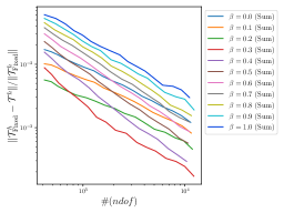
(a) $\theta=0.4$

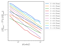
(b) $\theta=0.5$

(c) $\theta=0.6$

Figure 4: L-shape: Convergence study of ${\mathcal{E}}=\left\|\mathcal{T}^{h}_{\mathrm{Fixed}}-\mathcal{T}^{h}\right\|/\left\|\mathcal{T}^{h}_{\mathrm{Fixed}}\right\|$, using the $\eta=\sum_{i=1}^{3}\eta_{i}$ estimator for $\beta=0.0,\ldots,1.0$ (a) $\theta=0.4$ (b) $\theta=0.5$ (c) $\theta=0.6$.

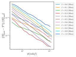
(a) $\theta=0.4$

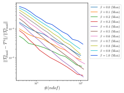
(b) $\theta=0.5$

(c) $\theta=0.6$

Figure 5: L-shape: Convergence study of ${\mathcal{E}}=\left\|\mathcal{T}^{h}_{\mathrm{Fixed}}-\mathcal{T}^{h}\right\|/\left\|\mathcal{T}^{h}_{\mathrm{Fixed}}\right\|$, using the $\eta=\max\eta_{i}$ estimator for $\beta=0.0,\ldots,1.0$ (a) $\theta=0.4$ (b) $\theta=0.5$ (c) $\theta=0.6$.

Comparing the results shown in Figures 4 and 5, we first observe that, unlike the results presented in Figures 2(a) and 2(b), changing $\beta$ can improve the convergence rate of ${\mathcal{E}}$ with respect to #$(ndof)$. For example, for $\theta=0.4$ and $\eta=\max\eta_{i}$, the convergence rate of ${\mathcal{E}}$ with respect to #$(ndof)$ can be improved from $-1.1$ to $-2.5$ by changing $\beta=0.2$ to $\beta=0.4$ (or from $-0.75$ to $-1.4$ considering ${\mathcal{E}}$ with respect to $1/h$), which can accelerate the convergence of the adaptive scheme. In particular, it can be observed that for both error estimators $\eta=\sum_{i=1}^{3}\eta_{i}$ and $\eta=\max\eta_{i}$, the the fastest convergence rate is obtained by choosing $\beta=0.4$, which also achieves small error values of ${\mathcal{E}}=0.00021$ for the finest mesh and $\theta=0.6$. Similar convergence curves for ${\mathcal{E}}$ were found for $\beta=0.5,0.6$, but with larger errors. We have repeated this study for a range of other objects and have found that in all cases the best performance in terms of convergence rate and accuracy for ${\mathcal{E}}$ were, among the parameters considered, for $0.3\leq\beta\leq 0.4$ and $k=10$.

5.2.2 Convergence Study for Varying Contrasts $k$

We have undertaken adaptive mesh approximations for different contrasts $k=0.1,0.2,1.5,10,15,100,150$ and summarise the $\beta$ for which the best results convergence rates were obtained using $\theta=0.6$ in Table 2.

Table 2: L-shape: Contrast $k$ and best $\beta$.

Contrast $k$	Best weight $\beta$	Measurement option
$0.1$	$0.0$	max
$0.2$	$0.4$	max
$1.5$	$0.6$	max
$10.0$	$0.4$	max
$15.0$	$0.3$	sum
$100.0$	$0.1$	sum
$150.0$	$0.1$	sum

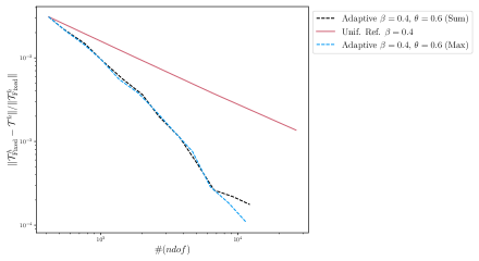
(a) Comparison of the relative error for $k=0.2$

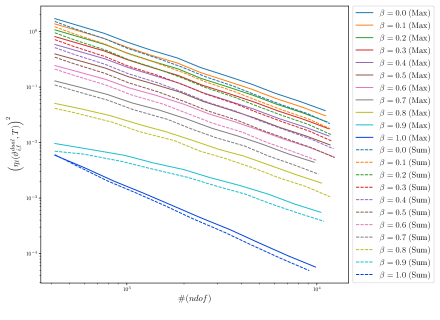
(b) ZZ-error estimator for $k=0.2$

Figure 6: L-shape: (a) Comparative study between uniform refinement and adaptive mesh solutions for ${\mathcal{E}}=\left\|\mathcal{T}^{h}_{\mathrm{Fixed}}-\mathcal{T}^{h}\right\|/\left\|\mathcal{T}^{h}_{\mathrm{Fixed}}\right\|$ for $\beta=0.4$, $\theta=0.6$ and $k=0.2$ (b) Convergence study of the ZZ-error estimator, using $\eta=\sum_{i=1}^{3}\eta_{i}$ and $\eta=\max\eta_{i}$ for $\beta=0.0,\ldots,1.0$, $\theta=0.6$ and $k=0.2$.

If adaptive mesh approximations for different contrasts $k=0.1,0.2,1.5,10$, $15,100,150$ are compared with uniform mesh refinements, we find that the adaptive algorithm offers a superior performance in terms of convergence rate and accuracy for ${\mathcal{E}}$ compared to uniform refinement for $k=0.1,0.2,1.5,10,15$ with the best performance for $k=0.1,0.2$. For $k=100,150$, the adaptive approach does not show an improvement over uniform refinement. We illustrate one of the best performing cases in terms of improvement in convergence rate and accuracy corresponding to $k=0.2$ in Figure 6(a) and show how error estimators $\eta=\sum_{i=1}^{3}\eta_{i}$ and $\eta=\max\eta_{i}$ converge for this case and different values of $\beta$ in Figure 6(b). In these experiments, a maximum of $25\,000$ surface triangles was generated by the adaptive algorithm while the uniform refinement led to $65\,536$ surface triangles.

5.2.3 Illustrations of Adaptive Meshes

For the case of $k=10$, the initial grid ${\mathcal{M}}_{0}$ and exemplar adaptive grids ${\mathcal{M}}_{\ell}$, $\ell=2,4,6$ obtained for $\beta=0.6$, $\theta=0.6$ using $\eta=\max\eta_{i}$ are shown in Figures 7(a)-7(d), respectively, which have $832$ to $6\,022$ surface triangles. Note that the meshes generated by the algorithm are more refined along the edges and corners, this trend is expected, since the solution $\phi_{i,h}$ is less regular at these locations and elements in the vicinity of edges and corners contribute most to the error estimate $\eta_{i}$. The distribution of the refined elements are similar for other objects.

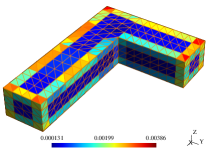
(a) Max - $\ell=0$

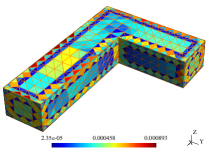
(b) Max - $\ell=2$

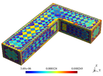
(c) Max - $\ell=4$

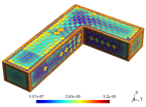
(d) Max - $\ell=6$

Figure 7: L-shape: Adaptive mesh generated using the ZZ-type error estimator using max direction measurement $\eta_{\ell}(\vartheta_{i}^{dual},T)$ for $\mathcal{M}^{dual}_{\ell}$ (a) $\ell=0$ (b) $\ell=2$ (c) $\ell=4$ (d) $\ell=6$.

5.2.4 Comparison of Computational Time

As an example of computational timings, the L-shape object with contrast $k=0.2$, weight $\beta=0.4$, and $\theta=0.6$ and a target accuracy of $\mathcal{E}\approx 1.3\times 10^{-3}$ is considered. The time taken by the adaptive mesh and the uniform mesh approaches is compared in Table 3, where a time saving of around 9 minutes can be observed. For this example, we have used the following machine Intel(R) Xeon(R) CPU E5-2687W v2 at 3.40GHz, 8 cores and 128 GB of RAM.

Table 3: L-shape: Computational time study.

Refinement approach	$\mathcal{E}$	$\#ndof$	Computational Time
Uniform Mesh	$1.376036530\times 10^{-3}$	$26\,626$	0:14:22
Adaptive Mesh	$1.330921701\times 10^{-3}$	$3\,412$	0:05:12

5.3 Reference Polarization Tensors and Benchmark Computations

The benchmark computations obtained using the adaptive mesh algorithm for each of the benchmark geometries in Section 5.1 are now presented for the case of $k=10$. We state ${\mathcal{E}}$ for each of the tensors resulting from the final adaptive mesh. In addition, by introducing the splitting

$${\mathcal{T}}={\mathcal{O}}+{\mathcal{D}},$$

where ${\mathcal{D}}$ is the diagonal part of ${\mathcal{T}}$ and ${\mathcal{O}}$ the off-diagonal part, we provide a measure of the error in the off-diagonal part of the tensor as

$$\mathcal{E}^{\mathrm{off}}:=\dfrac{\left\|\mathcal{O}^{h}_{\mathrm{Fixed}}-\mathcal{O}^{h}\right\|}{\left\|\mathcal{T}^{h}_{\mathrm{Fixed}}\right\|}.$$

for $\mathcal{T}^{h}$ obtained on the final adaptive mesh. The results are summarised in Table 4 for each benchmark geometry, using $\eta=\max\eta_{i}$ and $\theta=0.6$.

Table 4: Relative error and off-diagonal error for the best convergence result.

Object	Best $\beta$	Maximum	Number of elements	$\mathcal{E}$	$\mathcal{E}^{\mathrm{off}}$
		$\#ndof$	on $\mathcal{M}$	in %	in %
L-shape	$0.4$	$11\,681$	$23\,358$	$0.0213$	0.0019
Cube	$0.4$	$11\,522$	$23\,040$	$0.0013$	0.0001
Tetrahedron	$0.5$	$12\,078$	$24\,152$	$0.0170$	0.0140
Key	$0.3$	$17\,179$	$34\,354$	$0.0132$	0.0051

In the following sections, we present for each benchmark geometry the solution obtained with the smallest ${\mathcal{E}}$ from the adaptive mesh method with the PST coefficients arranged as a $3\times 3$ matrix in each case. Note that the solutions are restricted to a mesh with a maximum of $25\,000$ surface triangles, the only exception being the key object that the mesh can contain up to $40\,000$ surface triangles. We believe that at least the first four significant figures in our benchmark tensor characterisations are accurate.

5.3.1 L-shape: Best Approximation

The best approximation for the L-shape object is obtained for $\beta=0.4$, $\theta=0.6$ and $\eta=\max\eta_{i}$ and has a final adapted mesh with $23\,358$ surface triangles. This approximate tensor $\mathcal{T}^{h}$ is shown in (13)

$$\frac{\mathcal{T}^{h}}{10^{-4}}= \left(\begin{array}[]{ccc}\phantom{-}1.54683606\phantom{\times 10^{-6}}&-0.15091553\phantom{\times 10^{-6}}-6.99198691\times 10^{-6}\\ -0.15091553\phantom{\times 10^{-6}}&\phantom{-}1.16202896\phantom{\times 10^{-6}}\phantom{-}3.33569676\times 10^{-6}\\ -6.99198691\times 10^{-6}&\phantom{-}3.33569676\times 10^{-6}\phantom{-}0.57033981\phantom{\times 10^{-6}}\end{array}\right).$$ (13)

5.3.2 Cube: Best Approximation

For the cube object the best approximation is obtained by choosing $\beta=0.4$, $\theta=0.6$ and $\eta=\max\eta_{i}$ on a mesh with $23\,040$ surface triangles. This approximate tensor $\mathcal{T}^{h}$ is shown in (17)

$$\frac{\mathcal{T}^{h}}{10^{-6}}= \left(\begin{array}[]{ccc}\phantom{-}2.51110996\phantom{\times 10^{-6}}&\phantom{-}1.92945670\times 10^{-7}&-1.59571932\times 10^{-6}\\ \phantom{-}1.92945670\times 10^{-7}&\phantom{-}2.51111340\phantom{\times 10^{-6}}&-4.11272795\times 10^{-6}\\ -1.59571932\times 10^{-6}&-4.11272795\times 10^{-6}&\phantom{-}2.51110887\phantom{\times 10^{-6}}\end{array}\right).$$ (17)

5.3.3 Tetrahedron: Best Approximation

For the tetrahedron the best approximation is obtained by choosing $\beta=0.5$, $\theta=0.6$ and $\eta=\max\eta_{i}$ on a mesh with $24\,152$ surface triangles. This approximate tensor $\mathcal{T}^{h}$ is shown in (18)

$$\mathcal{T}^{h}=10^{-5}\begin{pmatrix}\phantom{-}9.30682676&1.12847255&-0.76359289\\ \phantom{-}1.12847255&6.83952305&\phantom{-}0.43032199\\ -0.76359289&0.43032199&\phantom{-}7.80618516\end{pmatrix}.$$ (18)

5.3.4 Key: Best Approximation

For the key the best approximation is obtained by choosing $\beta=0.3$, $\theta=0.6$ and $\eta=\max\eta_{i}$ on a mesh with $34\,354$ surface triangles. This approximate tensor $\mathcal{T}^{h}$ is shown in (22).

$$\frac{\mathcal{T}^{h}}{10^{-6}}= \left(\begin{array}[]{ccc}\phantom{-}2.66099087\phantom{\times 10^{-7}}&-2.40425167\times 10^{-2}&\phantom{-}1.94050498\times 10^{-5}\\ -2.40425167\times 10^{-2}&\phantom{-}4.49014335\phantom{\times 10^{-5}}&-3.78250864\times 10^{-6}\\ \phantom{-}1.94050498\times 10^{-5}&-3.78250864\times 10^{-6}&\phantom{-}0.96008445\phantom{\times 10^{-7}}\end{array}\right).$$ (22)

6 Conclusions

In this work, we have proposed a series of benchmark computations for the Póyla-Szegö tensor (PST) for different objects. We expect these benchmark computations to be of interest to electrical impedance tomography (EIT) practitioners, and, in particular, for those developing tools that will form part of a machine learning (ML) classification algorithm for detecting and classifying small conducting inclusions, but also to other computational partial differential equation solver developers.

PST object characterisations are attractive as they can easily be determined from voltage measurements in EIT, once the inclusion is known, by solving an over-determined linear system for their coefficients following from (1). This has advantages over a using voxelated grid and solving an ill-posed inverse problem for conductivity values in each voxel, which requires careful regularisation. However, in order for classification approaches based on PST object descriptions to work effectively, it is important that an accurate tool is used to compute the PST characterisations and our benchmark computations allow software developers to check that this is indeed the case. Nonetheless, a limitation of the PST object characterisation is that it only characterises an object up to the best fitting ellipsoid and does not allow the conductivity and the shape of the inclusion to be uniquely determined, which ultimately limits classification approaches built on PST descriptions. This can be improved by taking advantages of the spectral behaviour of PST coefficients by taking voltage measurements as a function of frequency, or, alternatively, by considering generalised polarizability tensor object characterisations, which include more information about an object’s shape and its materials.

We have presented a series of alternative boundary integral formulations, which, although identical for exact arithmetic, differ in practical computations for the computation of PST coefficients. We have described how these formulations can implemented in the boundary element method python package (Bempp). We have discussed how the application of an existing adaptive algorithm automates the refinement of the boundary element grid and reduces the computational effort required to compute the PST coefficients to a desired level of accuracy. We have included a series of numerical examples to demonstrate these benefits for objects with sharp corners and edges such as an L-shape domain, a cube, a tetrahedron and a key and explored how the conductivity constant effects the performance of the adaptive algorithm.

Appendix A Convergence of the Pólya-Szegö Tensor

In this section, a convergence result for the numerical approximation of ${\mathcal{T}}^{h}$ to ${\mathcal{T}}$ under uniform mesh refinement is presented.

In line with the solution to related boundary integral approximations of scalar Laplace transmission problems (e.g. [20, pg. 199, Proposition 4.1.31]), we conjecture that the approximate solution $\phi_{i}^{h}$ to $\phi_{i}$ satisfies the following a-priori type error estimate under uniform mesh refinement

$$\left\|\phi_{i}-\phi_{i}^{h}\right\|_{L^{2}(\Gamma)}\leq Ch^{s}\|\phi_{i}\|_{H^{s}(\Gamma)},0\leq s\leq 1.$$ (23)

It follows that we can establish that the convergence of the coefficients of the PST also have the same rate

$$\left\|{\mathcal{T}}-{\mathcal{T}}^{h}\right\|\leq Ch^{s},\quad 0\leq s\leq 1.$$

To show this, consider the coefficients of the exact PST ${\mathcal{T}}$, using the LP form, which are given by

$${\mathcal{T}}_{ij}=\int_{\Gamma}\xi_{j}\phi_{i}\,\mathrm{d}\bm{\xi}.$$

Let ${\mathcal{T}}^{h}_{ij}$ be a tensor computed numerically written as

$${\mathcal{T}}^{h}_{ij}=\int_{\Gamma}\xi_{j}\phi_{i}^{h}\,\mathrm{d}\bm{\xi},$$

where $\phi_{i}^{h}$ is an approximate solution computed using (7) and the effects of approximate numerical integration are ignored. Thus,

$$\left\|{\mathcal{T}}-{\mathcal{T}}^{h}\right\|= \left(\sum^{3}_{i,j=1}\left|{\mathcal{T}}_{ij}-{\mathcal{T}}^{h}_{ij}\right|^{2}\right)^{1/2}$$

$$= \left(\sum^{3}_{i,j=1}\left|\int_{\Gamma}\xi_{j}\left(\phi_{i}-\phi_{i}^{h}\right)\,\mathrm{d}\bm{\xi}\right|^{2}\right)^{1/2}$$

$$\leq \left(\sum^{3}_{i=1}\left|\int_{\Gamma}\left(\phi_{i}-\phi_{i}^{h}\right)\,\mathrm{d}\bm{\xi}\right|^{2}\right)^{1/2}\left(\sum^{3}_{j=1}\left|\int_{\Gamma}\xi_{j}\,\mathrm{d}\bm{\xi}\right|^{2}\right)^{1/2},$$

where the Cauchy-Schwarz inequality has been applied. This can be written as

$$\leq \left(\sum_{i=1}^{3}\left\|\phi_{i}-\phi_{i}^{h}\right\|_{L^{2}(\Gamma)}^{2}\right)^{1/2}\left(\sum_{j=1}^{3}\|\xi_{j}\|_{L^{2}(\Gamma)}^{2}\right)^{1/2}.$$

Note that, $\|\xi_{j}\|_{L^{2}(\Gamma)}\leq C$ with $C$ independent of $h$ and then we have

$$\left\|{\mathcal{T}}-{\mathcal{T}}^{h}\right\|\leq C\left(\sum^{3}_{i=1}\left\|\phi_{i}-\phi_{i}^{h}\right\|_{L^{2}(\Gamma)}^{2}\right)^{1/2}.$$ (24)

Substituting the error estimate in (23) into (24), we have

$$\left\|{\mathcal{T}}-{\mathcal{T}}^{h}\right\|\leq Ch^{s}\max_{i=1,2,3}\|\phi_{i}\|_{H^{s}(\Gamma)},$$

with $C$ independent of $h$. Note that,

$$\|\phi_{i}\|_{H^{s}(\Gamma)}\leq C,$$

where the constant $C$ depends of the shape of $B$, but not on $h$. Hence leading to the quoted result.

References

- [1] W. R. B. Lionheart, EIT reconstruction algorithms: pitfalls, challenges and recent developments, Physiological Measurement 25 (2004) 125–142.
- [2] J. L. Mueller, S. Siltanen, Linear and Nonlinear Inverse Problems with Practical Applications, Society for Industrial and Applied Mathematics, Philadelphia, PA, 2012.
- [3] A. Calderón, On an inverse boundary value problem, Computational and Applied Mathematics 25 (2-3) (2006) 133–138, reprinted from the Seminar on Numerical Analysis and its Applications to Continuum Physics, Sociedade Brasileira de Matemática, Rio de Janeiro, 1980.
- [4] E. T. Chung, T. F. Chan, X. C. Tai, Electrical impedance tomography using level set representation and total variational regularization, Journal of Computational Physics 205 (1) (2005) 357–372.
- [5] M. Hintermüller, A. Laurain, A. A. Novotny, Second-order topological expansion for electrical impedance tomography, Advances in Computational Mathematics 36 (2) (2012) 235–265.
- [6] T. Rymarczyk, G. Kłosowski, E. Kozłowski, A non-destructive system based on electrical tomography and machine learning to analyze the moisture of buildings, Sensors 18 (2018) 1–21.
- [7] D. J. Cedio-Fengya, S. Moskow, M. S. Vogelius, Identification of conductivity imperfections of small diameter by boundary measurements. continuous dependence and computational reconstruction, Inverse Problems 14 (1998) 553–595.
- [8] H. Ammari, H. Kang, Polarization and Moment Tensors: With Applications to Inverse Problems, Applied Mathematical Sciences, Springer-Verlag, New York, 2007.
- [9] P. D. Ledger, W. R. B. Lionheart, The perturbation of electromagnetics fields at distances that are large compared with the object’s size, IMA Journal of Applied Mathematics 80 (2015) 865–892.
- [10] T. A. Khairuddin, W. R. B. Lionheart, Characterization of objects by electrosensing fish based on the first order polarization tensor, Bioinspiration & Biomimetics 11 (5) (2016) 055004.
- [11] P. D. Ledger, W. R. B. Lionheart, Characterising the shape and material properties of hidden targets from magnetic induction data, IMA Journal of Applied Mathematics 80 (2015) 1776–1798.
- [12] C. M. Bishop, Pattern Recognition and Machine Learning, Springer, 2006.
- [13] B. A. Wilson, P. D. Ledger, W. R. B. Lionheart, Identification of metallic objects using spectral magnetic polarizability tensor signatures: Object classification, International Journal for Numerical Methods in Engineering 123 (2022) 2076–2111.
- [14] T. A. Khairuddin, W. R. B. Lionheart, Computing the first order polarization tensor: Welcome BEM++!, Discovering Mathematics (Menemui Matematik) 35 (2) (2013) 15–20.
- [15] W. Śmigaj, T. Betcke, S. Arridge, J. Phillips, M. Schweiger, Solving boundary integral problems with BEM++, ACM Transactions on Mathematical Software 41 (2) (2015) 6:1–6:40.
- [16] T. Betcke, A. Haberl, D. Praetorius, Adaptive boundary element methods for the computation of the electrostatic capacity on complex polyhedra, Journal of Computational Physics 397 (2019) 108837.
- [17] T. Betcke, M. W. Scroggs, W. Śmigaj, Product algebras for Galerkin discretisations of boundary integral operators and their applications, ACM Transactions on Mathematical Software 46 (2020) (2020).
- [18] S. Erichsen, S. A. Sauter, Efficient automatic quadrature in 3-d Galerkin BEM, Computer Methods in Applied Mechanics and Engineering 157 (1998) 215–224.
-
[19]
A. A. S. Amad, P. D. Ledger, T. Betcke, D. Praetorius,
Data set for the article
”Accurate benchmark polarizability tensor characterisations of small
conducting inclusions” (Oct. 2021).
doi:10.5281/zenodo.5591094.
URL https://doi.org/10.5281/zenodo.5591094 - [20] S. A. Sauter, C. Schwab, Boundary Element Methods, Springer Series in Computational Mathematics, Springer, Berlin, 2011.