INN: A Method Identifying Clean-annotated Samples via Consistency Effect in Deep Neural Networks

Abstract

In many classification problems, collecting massive clean-annotated data is not easy, and thus a lot of researches have been done to handle data with noisy labels. Most recent state-of-art solutions for noisy label problems are built on the small-loss strategy which exploits the memorization effect. While it is a powerful tool, the memorization effect has several drawbacks. The performances are sensitive to the choice of a training epoch required for utilizing the memorization effect. In addition, when the labels are heavily contaminated or imbalanced, the memorization effect may not occur in which case the methods based on the small-loss strategy fail to identify clean labeled data. We introduce a new method called INN (Integration with the Nearest Neighborhoods) to refine clean labeled data from training data with noisy labels. The proposed method is based on a new discovery that a prediction pattern at neighbor regions of clean labeled data is consistently different from that of noisy labeled data regardless of training epochs. The INN method requires more computation but is much stable and powerful than the small-loss strategy. By carrying out various experiments, we demonstrate that the INN method resolves the shortcomings in the memorization effect successfully and thus is helpful to construct more accurate deep prediction models with training data with noisy labels.

1 Introduction

Learning deep neural networks (DNNs) has achieved impressive successes in many research fields but has suffered from collecting massive clean-annotated training samples such as ImageNet [1] and MS-COCO [2]. Since annotating procedures are usually done manually by human experts, it is expensive and time-consuming to get large clean labeled data, which prevents deep learning models from being trained successfully. On the other hand, it is feasible to access numerous data through internet search engines [3, 4, 5, 6] or hashtags, whose labels are easy to collect but relatively inaccurate. Thus it becomes to get a spotlight to exploit data sets with corrupted labels instead of clean ones to solve classification tasks with DNNs, which is called the noisy label problem.

There have been many kinds of literature dealing with noisy labeled data, and a majority of methods exploited so-called the memorization effect, which is a special characteristic of DNNs that DNNs memorize data eventually (i.e. perfectly classify training data) but memorize clean labeled samples earlier and noisy samples later [7, 8]. Hence, we can identify clean data from the given training data contaminated with noisy labels by choosing samples with small loss values. Due to its simplicity and superiority, many follow-up studies have been proposed based on the small-loss strategy and achieved great success ([9] and references therein).

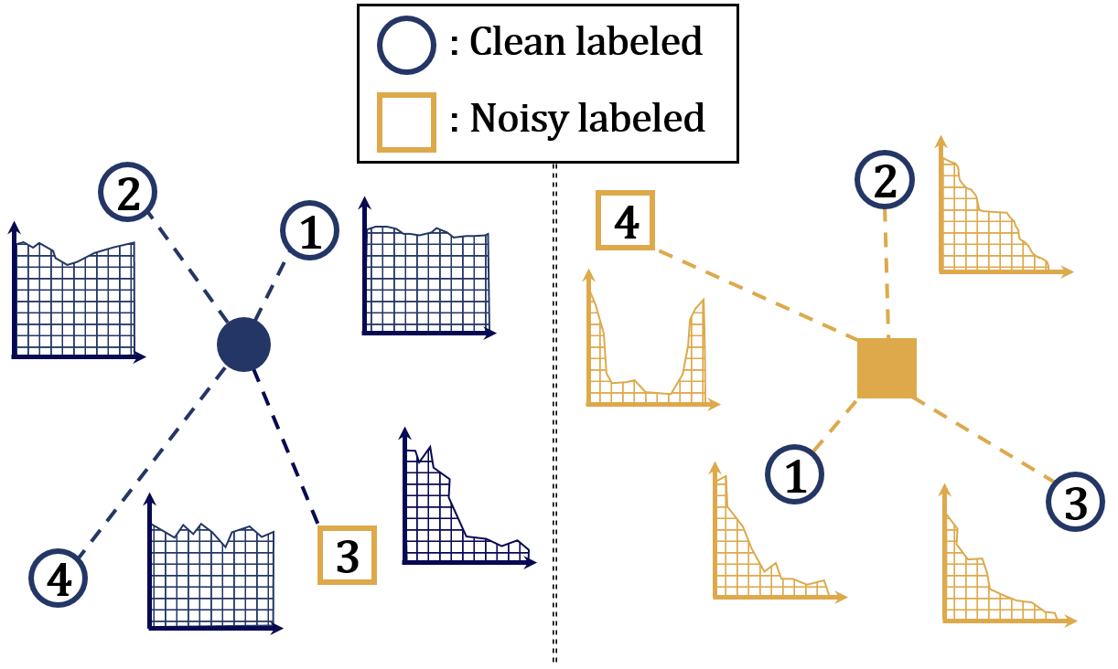
Figure 1: An illustration of the INN method. Circle and square are inputs with clean label and noisy label, respectively. Numbered dots are the nearest inputs. Each graph presents the value of a given prediction model along the dashed line. The INN method takes an average of the areas under each of the graphs.

But the small-loss strategy has several weaknesses. First, during the training phase, it is difficult to know a training epoch (or iteration) where the discrepancy of loss values between clean data and noisy data is large since it heavily depends on various factors including data set, model architecture, optimizer type and even learning schedule. Second, it becomes hard to identify clean-annotated samples from training data via the small-loss strategy when the training labels are heavily polluted. Besides, the memorization effect may not appear when we analyze the data with imbalanced label distribution. As we can obtain imbalanced data frequently in many real-world domains, this shortcoming can be an obstacle for the small-loss strategy applied in many industry fields.

To tackle these issues about the memorization effect, we develop a novel and powerful method called INN (Integration with the Nearest Neighbors). We start with a new and interesting observation that the output values of a trained DNN at neighbor regions of labeled and noisy samples are consistently much different regardless of training epochs. We call this phenomenon the consistency effect. Motivated by the consistency effect, the INN method takes averages of the output values of neighbor regions of a given sample and decides it as noisy if the average is small. See Figure 1 for an illustration of the INN method.

In fact, the INN requires more computation than the small-loss method. Still, this additional expense deserves to pay since the INN successfully overcomes the small-loss method’s limitations. The INN works well even when the training labels are heavily contaminated or has imbalanced distribution, while the small-loss method is in trouble for the situations. The stability and superiority make the INN easily applicable to various supervised learning tasks without much effort.

We can also combine the INN with an existing noisy-label-problem-solving learning method based on the small-loss strategy (e.g. DivideMix [10]) to construct deep networks of high accuracy. We replace the parts where the memorization effect and loss information are used with the consistency effect and the INN information. We show that these modifications enhance prediction performances much, especially when training labels have many noises or imbalanced distribution.

This paper is organized as follows. In Section 2, we provide brief reviews for related studies dealing with noisy labels, and detailed descriptions of the INN are given in Section 3. Various experimental analyses including performance test and ablation study are given in Section 4 and final concluding remarks follow in Section 5. The key contributions of this work are as follows.

• We find a new observation called the consistency effect, that the output values of a trained DNN at neighbor regions of labeled and noisy samples are consistently much different regardless of training epochs.

• Built on the consistency effect, we propose a method called the INN to identify clean annotated data from a given training data.

• We empirically demonstrate that the INN can separate clean and noisy samples accurately and stably even under the heavy label corruption and imbalanced label distribution, and also helpful to construct superior prediction models.

2 Related works

The noisy label problem has been studied for several decades [11, 12, 13]. The core issue to solve the noisy label problem with DNNs is that DNNs easily over-fit all training samples, including noisy labeled ones, because of too large complexities resulting in inferior generalization performances. Here we review some related studies for efficient algorithms to train robust classifiers in noisy annotations based on the key concepts called the loss correction and the memorization effect. And we also describe several approaches exploiting the information of a target sample’s neighborhoods as the INN does.

Loss correction based algorithms have a goal to improve the generalization error by modifying objective functions [14, 15]. The noise adaptive layer-based algorithm [16] added additional noisy channels that estimate the correct labels. The iterative noisy label detection [17, 18] used the weighted softmax loss function where the weights are updated iteratively based on the feature maps of the current DNN model. Some algorithms to estimate ground-truth labels directly have been developed [19, 20]. The meta-learning algorithm was also applied to resolve the noisy label problem [21]. There was an attempt to propose a new loss function more robust than standard loss functions [22].

Approaches based on the memorization effect focused on the gap between the output values of clean labeled and noisy labeled samples during an early stage of the training phase. The decouple method [23] proposed a meta-algorithm called decoupling which decides when to update. D2L [24] distinguished clean labeled data from noisy ones by employing a local dimensionality measure and ELR [25] found the faster gradient vanishings of clean labeled samples at the early learning stage. There were several algorithms to train noisy-robust prediction models by using only a subset of the training data based on their loss or prediction values. [26, 27, 28, 29, 30, 31]. Some studies fitted a two-component mixture model to a per-sample loss distribution [32, 10].

Some works tried to utilize the information of neighborhoods to filter out noisy labeled data, similar to the INN’s idea. The distance-weighted $k$-NN [33] was an initial work that considers the nearest samples with their distance-based weights. Deep $k$-NN [34] proposed a filtering strategy based on the label information of nearest neighbors, and MentorMix [35] applied MixUp [36] to MentorNet [8] to consider linear combinations of two inputs. We will discuss about the difference between the INN and the methods of exploiting neighbor’s information in Section 3.3.

3 Integration with the nearest neighbors

3.1 Notations and definitions

For a given input vector ${\bf x}\in\mathbb{R}^{d}$, let $y,y^{*}\in[K]$ be its observable and ground-truth labels, respectively, where $[K]=\{1,\ldots,K\}$. Of course, $y$ might be different from $y^{*}$. We say that the sample $({\bf x},y)$ is cleanly labeled if $y=y^{*}$ and noisily labeled if $y\neq y^{*}$. Let ${\cal D}^{\text{tr}}=\left\{({\bf x}_{i},y_{i})\right\}_{i=1}^{n}$ be a training data set with $n$ samples. Define ${\cal C}^{\text{tr}}=\{({\bf x},y)\in{\cal D}^{\text{tr}}:y=y^{*}\}$ and ${\cal N}^{\text{tr}}=\{({\bf x},y)\in{\cal D}^{\text{tr}}:y\neq y^{*}\}$. Our goal is to identify the clean labeled subset ${\cal C}^{\text{tr}}$ from ${\cal D}^{\text{tr}}$ accurately.

Let $f({\bf x};\theta):\mathbb{R}^{d}\to\mathbb{R}^{K}$ (abbr. $f({\bf x})$) be a discriminative DNN parametrized by $\theta$ which maps an input ${\bf x}$ to a $K$-dimensional conditional probability vector with the softmax layer. Also let $f_{k}({\bf x})$ be the $k$-th component of $f({\bf x})$, that is, we can represent $f({\bf x})$ as $(f_{1}({\bf x}),\ldots,f_{K}({\bf x}))$.

3.2 Consistency effect

Before we start, we explain the main motivation of our method. For a given training sample $({\bf x},y)\in{\cal D}^{\text{tr}}$, we define ${\bf x}^{\text{m}}=({\bf x}+\tilde{{\bf x}})/2$, where $\tilde{{\bf x}}$ is the nearest neighbor training input of ${\bf x}$ on the feature space $h(\cdot;\widehat{\eta})$ (i.e. $h(\tilde{{\bf x}};\widehat{\eta})$ is most close to $h({\bf x};\widehat{\eta})$) and $h(\cdot;\widehat{\eta})$ is the output of the penultimate layer of a pre-trained prediction model on ${\cal D}^{\text{tr}}$. Then, we can regard that ${\bf x}^{\text{m}}$ locates in the neighbor region of ${\bf x}$. We investigate how the prediction values of the training inputs and their neighbors behave differently by the label cleanness. We also estimate a prediction model $f({\bf x};\widehat{\theta})$ by minimizing the standard cross-entropy based on ${\cal D}^{\text{tr}}$. At each training epoch, we calculate the four expectations defined as

$$\begin{array}[]{ll}E_{\text{cor}}=\mathbb{E}_{({\bf x},y)\sim{\cal C}^{\text{tr}}}\left[f_{y}({\bf x})\right],&E_{\text{inc}}=\mathbb{E}_{({\bf x},y)\sim{\cal N}^{\text{tr}}}\left[f_{y}({\bf x})\right]\\ {E}_{\text{cor}}^{\text{m}}=\mathbb{E}_{({\bf x},y)\sim{\cal C}^{\text{tr}}}\left[f_{y}({\bf x}^{\text{m}})\right],&{E}_{\text{inc}}^{\text{m}}=\mathbb{E}_{({\bf x},y)\sim{\cal N}^{\text{tr}}}\left[f_{y}({\bf x}^{\text{m}})\right].\end{array}$$

Two values $E_{\text{cor}}$ and $E_{\text{inc}}$ are the expectations of clean and noisy data’s predictions, respectively, and ${E}_{\text{cor}}^{\text{m}}$ and ${E}_{\text{inc}}^{\text{m}}$ are the expectations of neighbor region’s prediction values over the clean and noisy labeled data, respectively. From Figure 3, we can see a typical phenomenon related to the memorization effect: $E_{\text{cor}}$ and $E_{\text{inc}}$ are much different at early epochs but the difference diminishes as the training epoch proceeds. That means that it becomes hard to discriminate noisy data from clean ones by comparing $f_{y}({\bf x})$ values at each sample at later stages of the training phase. But it is difficult to decide how many epochs are necessary for amply utilizing the memorization effect.

On the other hand, the difference between ${E}_{\text{cor}}^{\text{m}}$ and ${E}_{\text{inc}}^{\text{m}}$ is clearly significant regardless of training epochs. That is, the prediction values of neighbor regions for each sample are informative to separate clean and noisy data even when the number of training epoch is large. We call this new observation the consistency effect. This consistent discrepancy occurs by two reasons. First, when $({\bf x},y)$ is a noisy labeled sample, the label of an input ${\bf x}$, i.e. $y$, and the label of its neighborhood training sample $\tilde{{\bf x}}$ denoted by $\tilde{y}$ tend not to coincide, which yields the small prediction value $f_{y}({\bf x}^{\text{m}})$. And even if $y$ and $\tilde{y}$ are equal, $\tilde{{\bf x}}$ may not be the nearest neighbor on the input space (i.e. $\tilde{{\bf x}}$ is not close to ${\bf x}$). Hence, there exists a region between ${\bf x}$ and $\tilde{{\bf x}}$ at which the value of $f_{y}(\cdot)$ becomes small.

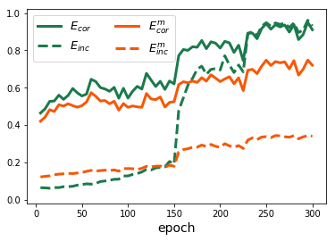
Figure 2: Comparison of $E_{\text{cor}}$, $E_{\text{inc}}$, ${E}_{\text{cor}}^{\text{m}}$ and ${E}_{\text{inc}}^{\text{m}}$ for various training epochs. We use the 30% symmetrically noisy CIFAR10 as ${\cal D}^{\text{tr}}$.

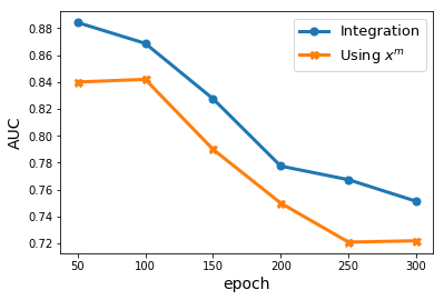
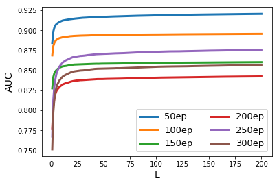
Figure 3: Comparison of AUC values for clean/noisy sample classification of the INN by varying some factors. We consider about (Left) how to utilize the prediction information of neighbor regions and (Right) the number of the nearest neighborhoods. We use the 40% asymmetrically noisy CIFAR10 as ${\cal D}^{\text{tr}}$

3.3 INN method

In this section, we propose a new and novel method to identify clean labeled samples motivated by the consistency effect. As being observed in Section 3.2, it is important to take into account the prediction values at a neighbor region of each sample. Let $f(\cdot;\widehat{\theta})$ be a prediction model trained with a loss function $l$ on ${\cal D}^{\text{tr}}$ for $T^{\text{inn}}$ training epochs. In this study, we use the MixUp objective function [36] as the loss function $l$. For a given training sample ${\bf z}=({\bf x},y)\in{\cal D}^{\text{tr}}$ and its neighborhood training input $\tilde{{\bf x}}$, a naturally induced score to identify whether $y$ is clean or not would be $I({\bf x};\widehat{\theta},\tilde{{\bf x}}):=f_{y}({\bf x}^{\text{m}};\widehat{\theta})$, where ${\bf x}^{\text{m}}=({\bf x}+\tilde{{\bf x}})/2$. From further experiments, we modify the score as follows. First, it is observed that the consistency effect occurs at many input vectors between ${\bf x}$ and $\tilde{{\bf x}}$ other than ${\bf x}^{\text{m}}$. Thus, to exploit the consistency effect fully, we consider integrating the prediction function over the whole interval between ${\bf x}$ and $\tilde{{\bf x}}$ to have

$$I({\bf x};\widehat{\theta},\tilde{{\bf x}})=\int_{0}^{1}f_{y}\left(\alpha{\bf x}+(1-\alpha)\tilde{{\bf x}};\widehat{\theta}\right)d\alpha.$$

Second, using multiple neighbor samples helps identify clean labeled data more accurately. Based on these two arguments, we propose the INN score given as:

$$I({\bf z};\widehat{\theta},\tilde{{\cal X}})=\frac{1}{L}\sum_{l=1}^{L}\int_{0}^{1}f_{y}(\alpha{\bf x}+(1-\alpha\tilde{{\bf x}}_{l});\widehat{\theta})d\alpha,$$ (2)

where $\tilde{{\cal X}}=\{\tilde{{\bf x}}_{1},\ldots,\tilde{{\bf x}}_{L}\}$ is the set of $L$ nearest neighbor training inputs of ${\bf x}$ on the feature space described in Section 3.2. Figure 3 illustrates the effects of these two modifications. The integration in (2) can be easily approximated by the trapezoidal rule as follows:

$$\frac{1}{L}\sum_{l=1}^{L}\sum_{h=1}^{H}\frac{1}{2H}\left(f_{y}({\bf x}_{l,h-1};\widehat{\theta})+f_{y}({\bf x}_{l,h};\widehat{\theta})\right),$$

where ${\bf x}_{l,h}=\frac{H-h}{H}{\bf x}+\frac{h}{H}\tilde{{\bf x}}_{l}$ and $H$ is the number of trapezoids. In practice, we fix the value of $H$ and $L$ to 10. The larger the score $I({\bf z};\widehat{\theta},\tilde{{\cal X}})$ is, the more we could regard ${\bf z}$ as being cleanly labeled. Hereafter, we will abbreviate $I({\bf z};\widehat{\theta},\tilde{{\cal X}})$ to $I({\bf z})$. Even after large training epochs, since there still remains the consistency effect in the prediction model, the INN method separates clean labeled data from noisy ones well. The following simple lemma supports the validity of our method.

Lemma 1.

Let $f:\mathbb{R}^{d}\to\mathbb{R}^{K}$ be a prediction model which perfectly over-fits the MixUp loss function

$$\mathbb{E}_{({\bf x}_{1},y_{1}),({\bf x}_{2},y_{2})\sim{\cal D}^{tr}}\mathbb{E}_{\lambda\sim B(\alpha,\alpha)}\left[\text{CE}\left(\text{mix}_{\lambda}(y_{1},y_{2}),f(\text{mix}_{\lambda}({\bf x}_{1},{\bf x}_{2})\right)\right],$$

where CE is the cross-entropy loss function, $\text{mix}_{\lambda}(a,b)=\lambda a+(1-\lambda)b$, and $B(\alpha,\alpha)$ is the Beta distribution with a hyperparameter $\alpha>0$. Also let assume that for each training input ${\bf x}$, its nearest neighbor set ${\cal X}=\{\tilde{{\bf x}}_{1},\ldots,\tilde{{\bf x}}_{L}\}$ satisfies $\text{argmax}_{k\in[K]}\sum_{l=1}^{L}I(\tilde{y}_{l}=k)=y^{*}$, where $\tilde{y}_{l}$ is the observed label of $\tilde{{\bf x}}_{l}$ and $y^{*}$ is the ground-truth label of ${\bf x}$. Then, the following inequality holds:

$$\min_{{\bf z}\in{\cal C}^{tr}}I({\bf z})>\max_{{\bf z}\in{\cal N}^{tr}}I({\bf z}).$$

Algorithm 1 INN (In practice, we fix $L$ to 10.)

0:  Training data ${\cal D}^{\text{tr}}=\{({\bf x}_{i},y_{i})\}_{i=1}^{n}$, a prediction model $f(\cdot;{\theta})$, a pre-trained feature model $h(\cdot;\widehat{\eta})$, the number of neighborhoods $L$, a training epoch $T^{\text{inn}}$, an optimizer ${\cal O}$

1:  $D(\cdot,\cdot)\leftarrow L_{2}(h(\cdot;\widehat{\eta}),h(\cdot;\widehat{\eta}))$ //dissimilarity measure

2:  for $t=1$ to $T^{\text{inn}}$ do

3:     $\widehat{\theta}\leftarrow MixUp(f(\cdot;\theta),{\cal D}^{\text{tr}},{\cal O})$ //train $f$ using MixUp

4:  end for

5:  ${\cal S}\leftarrow\emptyset$ //Define INN score set

6:  for $i=1$ to $n$ do

7:     $\tilde{{\cal X}}_{i}=\{\tilde{{\bf x}}_{i1},\ldots,\tilde{{\bf x}}_{iL}\}\leftarrow neighbor({\bf x}_{i},D)$ //$L$ nearest neighborhoods of ${\bf x}_{i}$

8:     ${\bf z}_{i}\leftarrow({\bf x}_{i},y_{i})$

9:     $s_{i}\leftarrow I({\bf z}_{i};\widehat{\theta},\tilde{{\cal X}}_{i})$ //INN score of ${\bf z}_{i}$

10:     ${\cal S}\leftarrow\text{append}({\cal S},s_{i})$ //append $s_{i}$ to ${\cal S}$

11:  end for

11:  ${\cal S}=\{s_{i}\}_{i=1}^{n}$

The proof is in the supplementary materials. Lemma 1 means that if we have a prediction model trained with the MixUp and good nearest neighborhood sets, then the INN separates ${\cal C}^{tr}$ perfectly from ${\cal N}^{tr}$.

As mentioned in Section 2, there are several approaches similar to the INN that utilize the nearest neighborhoods’ information to filter out noisy data [17, 21, 34, 35]. They mainly take advantage of the labels of the neighborhoods. When the training labels are polluted heavily, most of the nearest samples also become noisy, thus relying only on the label information might lead to bad results. On the other hand, the INN focuses on the regions between the inputs and their neighbor training samples. So, we expect that the INN would be robust to highly noisy data.

The algorithm of the INN method is summarized in Algorithm 1.

4 Experimental analysis

In this section, we empirically show the superiority of the INN in terms of three aspects. First, the INN is not sensitive to the choice of the training epochs and provides consistent performances. Second, the INN is significantly better than the small-loss strategy when many polluted labels are in the training data. Finally, in a situation where the training labels are imbalanced, the small-loss strategy may not work, while our method still succeeds in finding clean labeled data. And we also provide a combination of the INN and an existing small-loss-based learning framework to construct better deep prediction networks. Some additional ablation studies follow after then.

4.1 Experimental settings

Data sets

We carry out extensive experiments including performance tests and ablation studies by analyzing three data sets, CIFAR10&100 [37] and Clothing1M [5]. Both CIFAR10 and CIFAR100 consist of 50K training data and 10K test data with an input size of $3\times 32\times 32$ all of which are cleanly labeled. Clothing1M is a large-scale data set with real-world noisy labels containing 1M training data collected from online shopping websites. We use the subset of the Clothing1M data set whose ground-truth labels are known. The subset consists of 48K samples with a noisy level of 20% roughly.

As for imposing noise labels to CIFAR10 and CIFAR100, we consider symmetric and asymmetric settings as other studies did [15, 20]. In the symmetric noise setting, for each sample in the training data set, its label is contaminated with a probability $r$ to a random label generated from the uniform distribution on $1$ to $K$ ($K=10$ for CIFAR10 and $K=100$ for CIFAR100). In the asymmetric noise setting for CIFAR10, with a probability $r$, a noisy label is generated by one of the following mappings: truck$\to$automobile, bird$\to$airplane, deer$\to$horse and cat$\leftrightarrow$dog. For CIFAR100, labels are asymmetrically contaminated by flipping a given label to the next label with a probability $r$ according to the transition chain: class1$\to$class2$\to\cdots\to$class100$\to$class1.

Architectures and implementation details

We need two models $f$ and $h$, and we use the same architectures for them in all experiments. For CIFAR10&100 we utilize PreActResNet18 (PRN, [38]) with randomly initialized weights, and for Clothing1M we use ResNet50 (RN, [39]) with pre-trained weights by ImageNet. We train all the deep networks using the SGD algorithm with a momentum of 0.9 and the mini-batch size of 128, set the initial learning rate as 0.02, and reduce it by a factor of 5 when the half and three-fourths of the learning procedure proceed, respectively. All the results of ours in the following experiments are the averaged values of three trials executed from random initial weights and mini-batch arrangements.

Figure 4: Comparison of AUC values for clean/noisy sample classification between the INN and the small-loss methods with two losses. The plot positioned at the $i$-th row from the top and the $j$-th column from the left is the result of the Case$i$-$j.$

4.2 Stability test of the INN

In this section, we show the stability and superiority of the INN for identifying clean labeled samples from training data. For CIFAR10&100, we consider eight cases (Case1-1 to Case4-2) by varying noise rates and noise types.

• CIFAR10 with (Case1-1) $r=0.1$ and (Case1-2) $r=0.3$ symmetrically noisy labels

• CIFAR10 with (Case2-1) $r=0.1$ and (Case2-2) $r=0.3$ asymmetrically noisy labels

• CIFAR100 with (Case3-1) $r=0.2$ and (Case3-2) $r=0.4$ symmetrically noisy labels

• CIFAR100 with (Case4-1) $r=0.1$ and (Case4-2) $r=0.2$ asymmetrically noisy labels

Figure 5: Comparison of AUC values for clean/noisy sample classification for Clothing1M.

We consider various training epochs for $f$, $T^{\text{inn}}$, from 50 to 300, and calculate the clean/noisy classification AUC values of the training data induced by the INN for each training epoch. We consider two small-loss methods for the baselines, whose loss functions are the standard cross-entropy (CE) and the sum of the cross-entropy and negative entropy (CE+NE), respectively. We evaluate the small-loss methods’ clean/noisy classification AUC values based on their per-sample losses.

The results are depicted in Figure 4. We can clearly see that the INN provides consistent and high-quality results for all considering cases regardless of training epochs. In contrast, the performances of other baselines become worse as the training epoch increases. That implies the INN gives a more stable and powerful performance for clean/noisy classification. We also repeat these experiments with another deep architecture, WideResNet28-2 [40], and leave the results in the supplementary materials.

As for Clothing1M, we extract the weights of $h$ from the estimate of RN pre-trained by ImageNet and train only $f$ for $T^{\text{inn}}$ epochs varying from 10 to 300. We compare the AUC values of the INN with those based on the loss values of RN trained by CE. Figure 5 shows that the INN is superior and more stable throughout the whole training procedure compared to the competitor, which again assures the effectiveness of the INN.

4.3 INN with heavy noisy rates

We experiment with situations where training data are highly contaminated with noisy labels. We analyze CIFAR10&100 and change their ground-truth labels with a high probability. Like the previous analysis, we compare the INN to the two small-loss-based methods trained with the CE and CE+NE, respectively.

The best clean/noisy classification AUC values of the training data for each method are summarized in Table 1. In the heavy noise case, the proportion of the clean labeled data is not large. Thus, reducing the loss of clean labeled data may not be an optimal direction to reduce the overall loss values in the early learning stages, leading to the degradation of the small-loss strategy. In contrast, the INN can still identify clean data from noisy ones effectively even when many noisy labels exist and outperform the small-loss methods with large margins. We conjecture that this performance differences arise because the consistency effect is more insensitive to the number of noisy labels.

Table 1: The best clean/noisy classification AUC values of the INN and small-loss methods. The averaged values over three trials are listed, and standard deviations are also given in the parenthesis.

Data set	CIFAR10		CIFAR100
Noise type	Symm.		Symm.		Asymm.
Noise rate ($r$)	0.8	0.9	0.8	0.9	0.4
CE	0.857 (0.011)	0.756 (0.015)	0.809 (0.005)	0.690 (0.009)	0.589 (0.002)
CE+NE	0.854 (0.012)	0.750 (0.017)	0.807 (0.015)	0.695 (0.011)	0.608 (0.003)
INN	0.885 (0.014)	0.817 (0.018)	0.853 (0.016)	0.717 (0.013)	0.671 (0.005)

4.4 Analysis of imbalanced data

We also analyze the noisy data where the ground-truth labels are imbalanced. In this section, we consider the two-class classification task. From CIFAR10, we randomly sample two classes: first and second labels are regarded as a majority class and a minority class, respectively. We gather all images in the first class and 10% randomly sampled images in the second class. We relabel the majority and minority classes to 0 and 1, respectively, i.e. $y^{*}\in\{0,1\}$, and for each sample, we flip its label with a probability of 0.3 to generate training data with noisy labels. We compare the normalized score distributions of the INN and the small-loss method (CE) with the training data. For each distribution, we make four histograms by considering two factors: 1) whether the ground-truth label is 0 or 1 and 2) whether the observed label is 0 or 1.

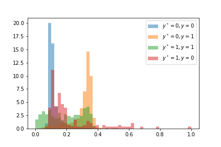
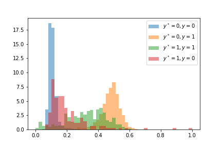
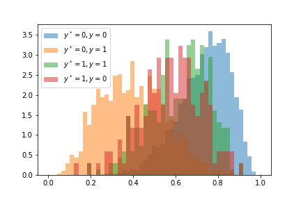
Figure 6: Score histograms for (Upper) the small-loss strategy (CE) and (Lower) the INN for imbalanced data. We fix the number of training epochs to 50 for the INN and 10 for the small-loss method. (Left to Right) We pick four class pairs, $(1,2),(3,8),(4,5)$ and $(7,9)$ and the first class for each pair is treated as a majority class. Data with $(y^{*},y)=(0,0),(0,1),(1,1)$ and $(1,0)$ are colored by blue, orange, green and red, respectively.

As can be seen in Figure 6, we observe that the model trained by the standard CE does not always prioritize memorizing the clean-labeled data anymore, i.e. data with $y=y^{*}$, rather memorizing the data with $y=0$, which implies the memorization effect may not occur in these imbalanced cases. Furthermore, their loss distributions are very unstable with respect to the training epochs. We report the histograms at other training epochs in the supplementary materials. In contrast, the consistency effect is still observable though not clear. The INN can separate clean samples from noisy ones to some extent, even if they belong to the minor class.

4.5 Constructing noise-robust classifiers

Table 2: Comparison of the test accuracies(%) of various method. The results marked with * are re-implemented by us and the other results except for INN$+$DivideMix are copied from the comparison table in [10] or their original papers. We only report the best results and attach the last accuracy results in the supplementary materials.

Data set	CIFAR10		CIFAR100
Noise type	Symm.		Symm.		Asymm.
Noise rate ($r$)	0.8	0.9	0.8	0.9	0.4
Cross-Entropy	62.9	42.7	19.9	10.1	42.7
Co-teaching$+$ [27]	67.4	47.9	27.9	13.7	-
P-correction [20]	77.5	58.9	31.1	15.3	-
MLNT [21]	-	59.1 (1.12)	-	-	-
M-correction [32]	86.8	69.1	48.2	24.3	-
DivideMix [10]	93.2	76.0	60.2	31.5	-
DivideMix*	92.90 (1.08)	71.34 (1.43)	58.26 (1.01)	31.36 (0.67)	59.26 (1.08)
INN$+$DivideMix	93.48 (1.01)	81.20 (1.05)	59.04 (0.98)	33.11 (0.82)	63.04 (1.10)

Table 3: The test accuracies(%) of the DivideMix and the modified DivideMix with the INN. The averaged values and standard deviations are reported.

Data set	Imbalanced CIFAR10
Classes	DivideMix		INN$+$DivideMix
	Best	Last	Best	Last
1 and 2	89.23 (0.40)	82.21 (0.57)	92.82 (0.27)	87.75 (0.77)
3 and 8	87.49 (0.68)	82.24 (1.65)	9 3.02 (0.12)	91.06 (0.18)
4 and 5	79.41 (0.68)	78.35 (0.98)	82.82 (0.20)	82.79 (0.13)
7 and 9	85.64 (0.35)	79.80 (1.92)	86.33 (0.45)	84.15 (0.25)

The INN is also helpful for learning deep classification models with high performance with noisy training data. Many conventional learning frameworks built on the small-loss strategy usually begin with learning models with the whole training data by minimizing the standard loss function, such as CE, for a few epochs. Due to the memorization effect, the early estimated models tend to memorize the clean-labeled training data first. Initialized with the estimated models, they conduct their own strategies to train models. After each training epoch, they update the per-sample loss values with the current model and utilize this information at the next training epoch.

We can modify them by simple modifications with the INN. First, we replace their initialized models with new ones trained with the INN. We fit a two-component mixture model to the INN scores of the training data and split the data into the labeled and unlabeled data based on the posterior probability of belonging to the clean cluster (the cluster with a larger mean). With the labeled and unlabeled data, we train prediction models for a few epochs using a semi-supervised learning method, such as the MixMatch [41], then use them as the initialized estimates. Second, after each training epoch, we recalculate the INN scores with the current prediction model and utilize these score values instead of the loss values at the next training epoch.

In this work, we provide an example to mix the INN and the DivideMix [10], known as one of the state-of-the-art methods to learning models with data mixed with noisy labels. We add a detailed algorithm of this combination in the supplementary materials. We again stress that any other small-loss-based learning frameworks than the DivideMix are also available to be combined with the INN to train better prediction models, and that there are many rooms to develop our simple application.

To assess the prediction performance of our modification, we analyze the same noisy data sets in Section 4.3 and 4.4. We carry out test accuracy comparison with the modified DivideMix with the INN (INN$+$DivideMix) and other baselines, which are reported in Table 2 and 3. We can check that our modified learning framework works better than the existing methods, including the DivideMix, in the cases where the training labels are highly polluted or imbalanced. And the performance gap between the best and last models trained with our method is smaller than the original DivideMix, which means the INN makes learning procedures more stable. We also make additional accuracy tests for data sets with noise rates not too severe and observe that ours gives no significant improvements since the DivideMix already works well. We report these results in the supplementary materials.

4.6 Ablation study

We empirically investigate how the choices of dissimilarity measure $h$ and the loss function $l$ affect the INN, whose detailed analyses are described in the supplementary materials. We observe that the Euclidean distance on the penultimate layer of a DNN trained by the training data is the best dissimilarity measure. And for the loss function, the MixUp objective function yields the best results.

We also evaluate the total training time of the INN and compare it to that of the standard small-loss method. We use a single NVIDIA TITAN XP GPU, and the results are in the supplementary materials. It takes much more time to implement the INN than the competitor since it needs to extract the nearest neighbors for each sample, which could be one of our limitations. More study to lighten the computation burden of the INN is required.

5 Concluding remarks

In this study, we proposed a new and novel approach, called the INN, to identify clean labeled samples from training data with noisy labels based on a new finding called the consistency effect that discrepancies of predictions at neighbor regions of clean and noisy data are consistently observed. We empirically demonstrated that the INN is stable and superior even when the training labels are heavily contaminated or imbalanced.

It would be interesting to apply our methods to unsupervised anomaly detection problems [42, 43, 44, 45]. After annotating labels (normal or abnormal) to the training data in a certain way, we can regard the task as the two-class noisy label problem. We expect that our methods would solve the anomaly detection problems successfully.

6 Supplementary materials for the INN

Supplementary materials for
INN: A Method Identifying Clean-annotated Samples via Consistency Effect in Deep Neural Networks

Appendix A Proof of Lemma 1

Let ${\bf z}=({\bf x},y)$ and $\tilde{{\bf X}}=\{\tilde{{\bf x}}_{1},\ldots,\tilde{{\bf x}}_{L}\}$ be a given training sample and a set of its nearest training inputs, respectively. Since the model $f$ perfectly over-fits the MixUp loss function, it is linear over between any two given training inputs. So, for $l=1,\ldots,L$ the following equality holds:

$$\int_{0}^{1}f_{y}(\alpha{\bf x}+(1-\alpha\tilde{{\bf x}}_{l});\widehat{\theta})d\alpha=\left\{\begin{array}[]{ll}1&\text{if }y=\tilde{y}_{l},\\ \frac{1}{2}&\text{otherwise,}\end{array}\right.$$

where $\tilde{y}_{l}$ is the corresponding observed label of $\tilde{{\bf x}}_{l}$. Hence, the INN score can be rewritten as:

$$I({\bf z})=\frac{1}{L}\sum_{l=1}^{L}\int_{0}^{1}f_{y}(\alpha{\bf x}+(1-\alpha\tilde{{\bf x}}_{l});\widehat{\theta})d\alpha=\frac{1}{L}\sum_{l=1}^{L}\left(I(y=\tilde{y}_{l})+\frac{1}{2}I(y\neq\tilde{y}_{l})\right).$$ (4)

By using $\text{argmax}_{k\in[K]}\sum_{l=1}^{L}I(\tilde{y}_{l}=k)=y^{*}$, we also have

$$\sum_{l=1}^{L}I(y^{*}=\tilde{y}_{l})\geq\frac{L}{K}\text{ and }\sum_{l=1}^{L}I(y^{*}\neq\tilde{y}_{l})\leq\frac{L-K}{K}.$$ (5)

With (4) and (5),

$$I({\bf z})\geq\frac{1}{L}\left[\frac{L}{K}+\frac{L-K}{2K}\right]\geq\frac{1}{L}\left(\frac{3L}{2K}-\frac{1}{2}\right)$$ (6)

if ${\bf z}$ is cleanly labeled, i.e. $y=y^{*}$, and

$$I({\bf z}) = \frac{1}{L}\sum_{l=1}^{L}\left(I(y=\tilde{y}_{l})+\frac{1}{2}I(y\neq\tilde{y}_{l})\right)$$ (7)

$$\leq \frac{1}{L}\sum_{l=1}^{L}\left(I(y^{*}\neq\tilde{y}_{l})+\frac{1}{2}\right)\leq\frac{1}{L}\left(\frac{L}{K}-\frac{1}{2}\right)$$

if ${\bf z}$ is noisy labeled. From (6) and (7), we have the following inequality and the proof is completed:

$$\underset{{\bf z}\in{\cal C}^{tr}}{\min}I({\bf z})-\underset{{\bf z}\in{\cal N}^{tr}}{\max}I({\bf z})\geq\frac{1}{2K}>0.\text{ $\square$ \par\vspace{.15in}}$$

Appendix B INN with another architecture

We carry out additional experiments for the performance test of the INN using another architecture. Here, we consider WideResNet28-2 [40] and we follow the main manuscript’s implementation settings, such as the strategies to impose noisy labels and learning schedules.

We depict the results in Figure B.1. Similar to the results with the PRN architecture, the clean/noisy classification performances of the INN are insensitive to the choice of the training epochs and consistently outperform other two competitors based on loss values.

Figure B.1: Comparison of AUC values for clean/noisy sample classification between the INN and the two small-loss methods. We utilize the WideResNet28-2 architecture. The plot positioned at the $i$-th row from the top and the $j$-th column from the left is the result of the Case$i$-$j$. As for the description of the eight cases, see the main manuscript.

Appendix C Instability of the small-loss method for imbalanced data

Figure C.1 illustrates histograms of the loss values at various training epochs when we analyze imbalanced data. The same data sets used in Section 4.4 of the main manuscript are considered. We can check that the loss distribution is unstable, so it is hard to choose an optimal training epoch.

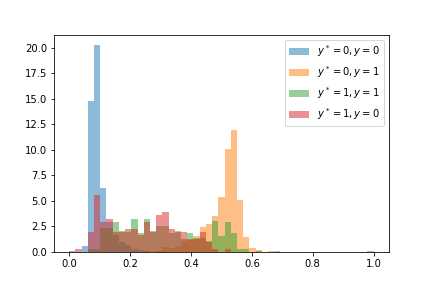
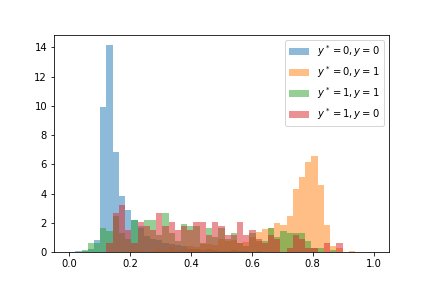
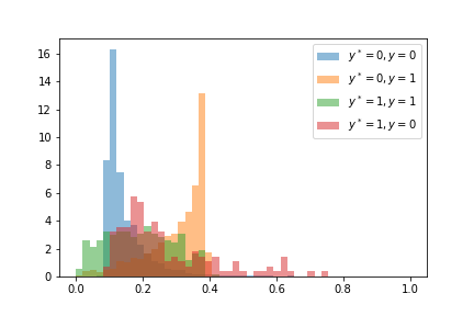
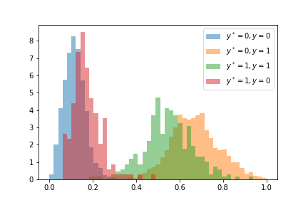
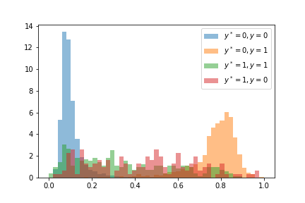
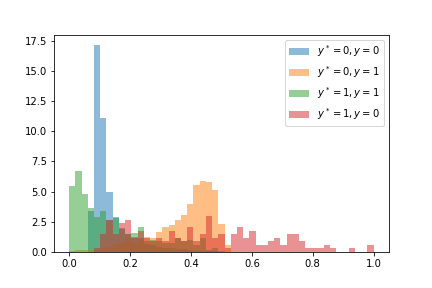
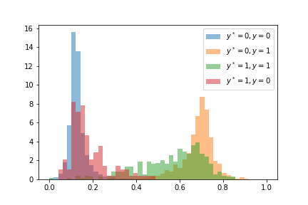
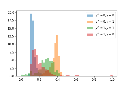
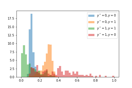
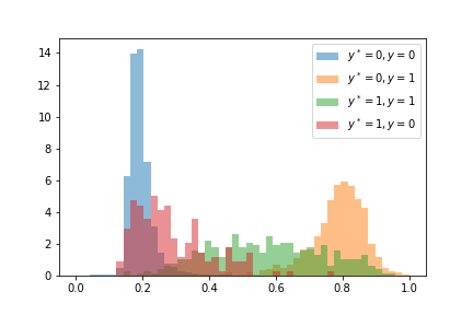
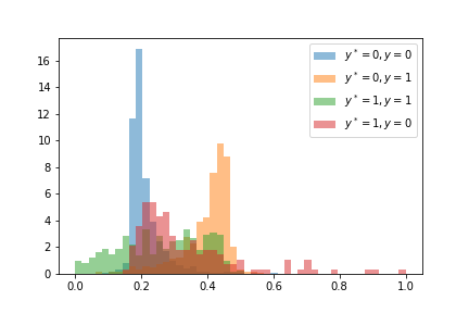
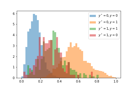
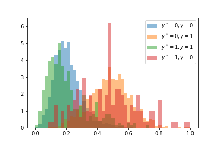
Figure C.1: The histograms of the loss value. (Upper to Lower) We consider five training epochs (1,5,10,15 and 20). (Left to Right) We pick four class pairs, $(1,2),(3,8),(4,5)$ and $(7,9)$, and the first class for each pair is treated as a majority class. Data with $(y^{*},y)=(0,0),(0,1),(1,1)$ and $(1,0)$ are colored by blue, orange, green and red, respectively.

Appendix D Modification of DivideMix with INN

D.1 Detailed algorithm description

Here, we describe our modification (INN$+$DivideMix) in detail by comparing it with the original DivideMix algorithm.

D.1.1 Step 1

Original DivideMix

The DivideMix trains two prediction models by minimizing the sum of the cross-entropy and negative entropy with two initial independent parameters for a pre-specified training epoch using the whole training data. The training epoch usually ranges from 10 to 30, depending on a data set. This part aims to get two initialization models robust to noisy labels to some extent via the memorization effect.

INN$+$DivideMix

First, we conduct the INN method twice to obtain two corresponding INN score sets of the training data with random initializations. With each INN score set, we separate the training data to labeled and unlabeled data by fitting a two-component Beta Mixture Model (BMM) to the INN scores using the Expectation-Maximization algorithm. We regard samples whose posterior probabilities of belonging to the clean cluster (the cluster with a larger mean) is larger than 0.5 as labeled data and treat the remained samples as unlabeled data by discarding their labels. Then, we utilize a semi-supervised learning (SSL) method to train two prediction models for a pre-specified training epoch with each pair of the labeled and unlabeled data. Any SSL method can be applied, and in our experiments, we adopt the MixMatch [46].

D.1.2 Step 2

Original DivideMix

The DivideMix updates two prediction models pre-trained from the first step. For each prediction model, the DivideMix fits a two-component Gaussian Mixture Model (GMM) on a per-sample loss distribution of the model to divide the training set into a labeled data set and an unlabeled data set, which is called the co-divide procedure. Then, the two models exchange the co-divided data sets and are trained based on the exchanged data sets by use of the SSL method modifying the MixMatch with the co-refinement and the co-guessing techniques. The DivideMix iterates the co-divide and the modified MixMatch method alternately for a pre-specified training epoch to construct the final prediction models.

INN$+$DivideMix

Similar to the original DivideMix, our method starts with two initialized prediction models from the first step of ours. For each prediction model, we calculate the INN score set. Note that we need a prediction model $f$ and a feature model $h$ to conduct the INN. Here, we set $f$ and $h$ to the current prediction model and its penultimate layer, i.e., the highest hidden layer, respectively. With each INN score set, we fit a two-component Beta Mixture Model (BMM) and split the training data into labeled and unlabeled data by using the posterior probabilities. Then, we utilize the same SSL algorithm used in the original DivideMix with the two pairs of labeled and unlabeled data sets to update the two prediction models. We repeat the above learning procedure for a pre-specified training epoch. We summarize our modification in Algorithm D.1. Algorithm D.1 requires three kinds of training epochs, $T_{1},T_{2},$ and $T_{3}$. In practice, we set $(T_{1},T_{2},T_{3})=(30,30,9)$ for all cases.

Algorithm D.1 INN+DivideMix: line 1-9: Step 1, line 10-20: Step 2

0:  Training data ${\cal D}^{\text{tr}}=\{({\bf x}_{1},y_{1}),\ldots,({\bf x}_{n},y_{n})\}$, two prediction models $g_{1}$ and $g_{2}$, three integers $T_{1},T_{2}$ and $T_{3}$, an optimizer ${\cal O}$

1:  Train two prediction models $f_{1}$ and $f_{2}$ and two feature models $h_{1}$ and $h_{2}$.

2:  ${\cal S}_{1}\leftarrow\{s_{11},\ldots,s_{1n}\}$; ${\cal S}_{2}\leftarrow\{s_{21},\ldots,s_{2n}\}$ //two INN score sets with $(f_{1},h_{1})$ and $(f_{2},h_{2})$, respectively

3:  ${\cal W}_{1}=\{w_{11},\ldots,w_{1n}\}\leftarrow\text{BMM}({\cal S}_{1})$; ${\cal W}_{2}=\{w_{21},\ldots,w_{2n}\}\leftarrow\text{BMM}({\cal S}_{2})$ //clean posterior probabilities

4:  ${\cal L}_{1}^{\text{tr}}=\{({\bf x}_{i},y_{i}):w_{1i}\geq 0.5,i=1,\ldots,n\}$; ${\cal U}_{1}^{\text{tr}}=\{{\bf x}_{i}:w_{1i}<0.5,i=1,\ldots,n\}$

5:  ${\cal L}_{2}^{\text{tr}}=\{({\bf x}_{i},y_{i}):w_{2i}\geq 0.5,i=1,\ldots,n\}$; ${\cal U}_{2}^{\text{tr}}=\{{\bf x}_{i}:w_{2i}<0.5,i=1,\ldots,n\}$ //two pairs of labeled and unlabeled data

6:  for $t_{1}=1$ to $T_{1}$ do

7:     $g_{1}\leftarrow\text{MixMatch}(g_{1},{\cal L}_{2}^{\text{tr}},{\cal U}_{2}^{\text{tr}},{\cal O})$

8:     $g_{2}\leftarrow\text{MixMatch}(g_{2},{\cal L}_{1}^{\text{tr}},{\cal U}_{1}^{\text{tr}},{\cal O})$ //conduct the MixMatch

9:  end for

10:  for $t_{2}=1$ to $T_{2}$ do

11:     $f_{1}\leftarrow g_{1}$; $h_{1}\leftarrow\text{penult}(g_{1})$ //update $f_{1}$ and $g_{1}$

12:     $f_{2}\leftarrow g_{2}$; $h_{2}\leftarrow\text{penult}(g_{2})$ //update $f_{2}$ and $h_{2}$

13:     ${\cal S}_{1}\leftarrow\{s_{11},\ldots,s_{1n}\}$; ${\cal S}_{2}\leftarrow\{s_{21},\ldots,s_{2n}\}$ //two INN score sets

14:     ${\cal W}_{1}=\{w_{11},\ldots,w_{1n}\}\leftarrow\text{BMM}({\cal S}_{1})$; ${\cal W}_{2}=\{w_{21},\ldots,w_{2n}\}\leftarrow\text{BMM}({\cal S}_{2})$ //clean posterior probabilities

15:     ${\cal L}_{1}^{\text{tr}}=\{({\bf x}_{i},y_{i}):w_{1i}\geq 0.5,i=1,\ldots,n\}$; ${\cal U}_{1}^{\text{tr}}=\{{\bf x}_{i}:w_{1i}<0.5,i=1,\ldots,n\}$

16:     ${\cal L}_{2}^{\text{tr}}=\{({\bf x}_{i},y_{i}):w_{2i}\geq 0.5,i=1,\ldots,n\}$; ${\cal U}_{2}^{\text{tr}}=\{{\bf x}_{i}:w_{2i}<0.5,i=1,\ldots,n\}$ //two pairs of labeled and unlabeled data

17:     for $t_{3}=1$ to $T_{3}$ do

18:        $g_{1},g_{2}\leftarrow\text{DivideMix-SSL}(g_{1},g_{2},{\cal L}_{1}^{\text{tr}},{\cal L}_{2}^{\text{tr}},{\cal U}_{1}^{\text{tr}},{\cal U}_{2}^{\text{tr}},{\cal O})$ //conduct the SSL part of the DivideMix

19:     end for

20:  end for

20:  $g_{1}$ and $g_{2}$ //final outputs

D.2 Performance tests of INN$+$DivideMix

We report the last test accuracy results of the INN$+$DivideMix on severely contaminated data sets. Table D.1 shows that the modified DivideMix with the INN improves the DivideMix with large margins.

The prediction performance of the INN in ordinary cases where there are not many noisy labeled samples in the training data are provided in Table D.2. Our modification does not give visible enhancement in these situations since the DivideMix already works well, so there is not much room to develop the original one.

Table D.1: Comparison of the last test accuracies(%) of various methods on severely polluted data sets. The averaged values (and standard deviations) are listed. The results marked with * are re-implemented by us and the other results except for INN$+$DivideMix are copied from the comparison table in [10] or their original papers.

Data set	CIFAR10		CIFAR100
Noise type	Symm.		Symm.		Asymm.
Noise rate ($r$)	0.8	0.9	0.8	0.9	0.4
Cross-Entropy	26.1	16.8	8.8	3.5	-
Co-teaching$+$ [27]	45.5	30.1	15.5	8.8	-
P-correction [20]	76.5	58.2	20.7	8.8	-
MLNT [21]	-	-	-	-	-
M-correction [32]	86.6	68.7	47.6	20.5	-
DivideMix [10]	92.9	75.4	59.6	31.0	-
DivideMix*	92.71(1.02)	68.79(1.31)	57.78(1.07)	31.16(1.21)	53.79(1.09)
INN$+$DivideMix	93.04(1.19)	80.51(1.05)	58.81(1.22)	32.36(0.86)	59.34(0.94)

Table D.2: Comparison of the best (and last) test accuracies(%) of various methods on data sets polluted not much. The results marked with * are re-implemented by us and the other results except for INN$+$DivideMix are copied from the comparison table in [10] or their original papers.

Data set	CIFAR10				CIFAR100
Noise type	Symm.				Symm.
Noise rate ($r$)	0.2	0.4	0.5	0.6	0.2	0.4	0.5	0.6
Cross-Entropy	86.8(82.7)	-	79.4(57.9)	-	62.0(61.8)	-	46.7(37.3)	-
Co-teaching$+$ [27]	89.5(88.2)	-	85.7(84.1)	-	65.6(64.1)	-	51.8(45.3)	-
P-correction [20]	92.4(92.0)	-	89.1(88.7)	-	69.4(68.1)	-	57.5(56.4)	-
MentorNet [8]	92.0(-)	89.0(-)	-	-	73.0(-)	68.0(-)	-	-
D2L [47]	85.1(-)	83.4(-)	-	72.8(-)	62.2(-)	52.0(-)	-	42.3(-)
MLNT [21]	92.9(92.0)	-	89.3(88.8)	-	68.5(67.7)	-	59.2(58.0)	-
Reweight [48]	86.9(-)	-	-	-	61.3(-)	-	-	-
Abstention [18]	93.4(-)	90.9 (-)	-	87.6(-)	75.8(-)	68.2(-)	-	59.4(-)
M-correction [32]	94.0(93.8)	-	92.0(91.9)	-	73.9(73.4)	-	66.1(65.4)	-
DivideMix [10]	96.1(95.7)	94.9(-)	94.6(94.4)	94.3(-)	77.3(76.9)	75.2(-)	74.6(74.2)	72.0(-)
DivideMix*	96.08(95.68)	94.95(94.51)	94.81(94.13)	94.29(93.95)	77.23(76.84)	74.92(74.12)	74.08(73.56)	72.58(71.99)
INN$+$DivideMix	96.11(95.82)	95.01(94.86)	94.99(94.83)	94.87(94.56)	77.27(76.86)	74.67(74.14)	75.18(74.83)	72.69(72.21)

Appendix E Detailed descriptions of ablation studies

E.1 Dissimilarity measure

As a dissimilarity measure, we utilize the Euclidean ($L_{2}$) distance between the feature representations (the penultimate layer representations) generated by a pre-trained prediction model, $D(\cdot,\cdot)=L_{2}(h(\cdot;\widehat{\eta}),h(\cdot;\widehat{\eta}))$, where $h(\cdot;\widehat{\eta})$ is the highest feature output of a pre-trained prediction model parametrized by $\widehat{\eta}$. Here, $\widehat{\eta}$ is trained by minimizing the standard cross-entropy (CE) function on ${\cal D}^{\text{tr}}$. As an alternative feature representation, we consider using an external training data set such as ImageNet. We obtain another feature representation by training $\eta$ based on the ImageNet data set (${\cal D}^{\text{IN}}$) and compare two representation output functions trained on 1) ${\cal D}^{\text{tr}}$ and 2) ${\cal D}^{\text{IN}}$, respectively by evaluating AUC values of their corresponding INN scores. The integrand prediction model $f(\cdot;\widehat{\theta})$ used in the formula (1) of the main manuscript is trained by minimizing CE based on ${\cal D}^{\text{tr}}$ with the maximum training epochs 300. By each 50 training epoch, we calculate the INN scores on ${\cal D}^{\text{tr}}$ with $L=10$ and evaluate the AUC values for the clean/noisy sample classification problem. The results are depicted in the left panel of Figure E.1, which show that using feature representations trained with the given training data set (${\cal D}^{\text{tr}}$) gives similar results.

E.2 Loss function

We investigate two loss functions to estimate the prediction model $f(\cdot;\widehat{\theta})$: 1) the standard cross-entropy (CE) function and 2) the MixUp (MU) objective function [36]. By each 50 training epoch, we calculate their INN scores on the training data and evaluate their AUC values. The right panel in Figure E.1 shows that the AUC values derived by the MU function are higher and relatively stable.

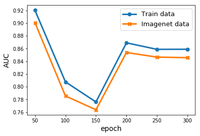
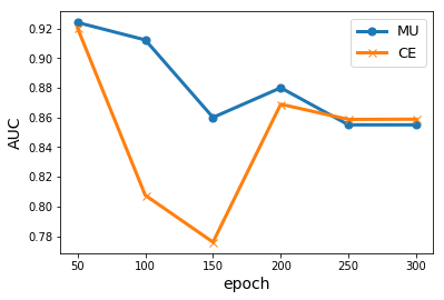
Figure E.1: AUC values for clean/noisy sample classification of the INN method obtained by varying two settings: (Left) training data set for learning $h$ and (Right) loss function for $f$. We analyze the 40% asymmetrically noisy CIFAR10.

E.3 Training time analysis

We analyze the total training time of the INN over CIFAR10 and compare it to the small-loss competitor. We use a single NVIDIA TITAN XP GPU and the results are summarized in Table E.1 and E.2. The elapsed time of the INN is two times longer than that of the small-loss method since investigating the nearest neighborhoods requires much more time than other steps. Thus, to overcome the limitation of the INN in terms of elapsed time, we need to modify and lighten the procedure to calculate neighborhoods.

Table E.1: Total elapsed time for running the INN. We train two deep architectures ($f$ and $h$) for 50 epochs by minimizing the MixUp loss function.

Training two architectures	Searching the nearest neighbors	Calculating the INN scores	Total
21.5sec/ep$\times$50ep	2520.4sec	890.9sec	4486.3sec

Table E.2: Total elapsed time for running the small-loss strategy. We train a deep architecture for 50 epochs by minimizing the sum of the cross-entropy and negative entropy.

Training an architecture	Calculating the loss scores	Total
40.2sec/ep$\times$50ep	3.8sec	2013.8sec

References

- [1] Jia Deng, Wei Dong, Richard Socher, Li-Jia Li, Kai Li, and Li Fei-Fei. Imagenet: A large-scale hierarchical image database. In 2009 IEEE Conference on Computer Vision and Pattern Recognition, pages 248–255, 2009.
- [2] Tsung-Yi Lin, Michael Maire, Serge Belongie, James Hays, Pietro Perona, Deva Ramanan, Piotr Dollár, and C Lawrence Zitnick. Microsoft coco: Common objects in context. In European Conference on Computer Vision, pages 740–755, 2014.
- [3] Rob Fergus, Li Fei-Fei, Pietro Perona, and Andrew Zisserman. Learning object categories from internet image searches. Proceedings of the IEEE, 98(8):1453–1466, 2010.
- [4] Florian Schroff, Antonio Criminisi, and Andrew Zisserman. Harvesting image databases from the web. IEEE Transactions on Pattern Analysis and Machine Intelligence, 33(4):754–766, 2010.
- [5] Tong Xiao, Tian Xia, Yi Yang, Chang Huang, and Xiaogang Wang. Learning from massive noisy labeled data for image classification. In 2015 IEEE Conference on Computer Vision and Pattern Recognition (CVPR), pages 2691–2699, 2015.
- [6] Jonathan Krause, Benjamin Sapp, Andrew Howard, Howard Zhou, Alexander Toshev, Tom Duerig, James Philbin, and Li Fei-Fei. The unreasonable effectiveness of noisy data for fine-grained recognition. In European Conference on Computer Vision, pages 301–320. Springer, 2016.
- [7] Devansh Arpit, Stanisław Jastrzębski, Nicolas Ballas, David Krueger, Emmanuel Bengio, Maxinder S Kanwal, Tegan Maharaj, Asja Fischer, Aaron Courville, Yoshua Bengio, et al. A closer look at memorization in deep networks. In International Conference on Machine Learning, pages 233–242. PMLR, 2017.
- [8] Lu Jiang, Zhengyuan Zhou, Thomas Leung, Li-Jia Li, and Li Fei-Fei. Mentornet: Learning data-driven curriculum for very deep neural networks on corrupted labels. In International Conference on Machine Learning, pages 2304–2313. PMLR, 2018.
- [9] Hwanjun Song, Minseok Kim, Dongmin Park, and Jae-Gil Lee. Learning from noisy labels with deep neural networks: A survey. arXiv preprint arXiv:2007.08199, 2020.
- [10] Junnan Li, Richard Socher, and Steven CH Hoi. Dividemix: Learning with noisy labels as semi-supervised learning. In 8th International Conference on Learning Representations, 2020.
- [11] Dana Angluin and Philip Laird. Learning from noisy examples. Machine Learning, 2:343–370, 1988.
- [12] Xingquan Zhu and Xindong Wu. Class noise vs. attribute noise: A quantitative study. Artificial Intelligence Review, 22:177–210, 2004.
- [13] David F Nettleton, Albert Orriols-Puig, and Albert Fornells. A study of the effect of different types of noise on the precision of supervised learning techniques. Artificial Intelligence Review, 33:275–306, 2010.
- [14] Giorgio Patrini, Alessandro Rozza, Aditya Krishna Menon, Richard Nock, and Lizhen Qu. Making deep neural networks robust to label noise: A loss correction approach. In 2017 IEEE Conference on Computer Vision and Pattern Recognition (CVPR), pages 2233–2241, 2017.
- [15] Zhilu Zhang and Mert Sabuncu. Generalized cross entropy loss for training deep neural networks with noisy labels. In 32nd International Conference on Neural Information Processing Systems, pages 8792–8802, 2018.
- [16] Jacob Goldberger and Ehud Ben-Reuven. Training deep neural-networks using a noise adaptation layer. In 5th International Conference on Learning Representations, 2017.
- [17] Yisen Wang, Weiyang Liu, Xingjun Ma, James Bailey, Hongyuan Zha, Le Song, and Shu-Tao Xia. Iterative learning with open-set noisy labels. In 2018 IEEE Conference on Computer Vision and Pattern Recognition, pages 8688–8696, 2018.
- [18] Sunil Thulasidasan, Tanmoy Bhattacharya, Jeff Bilmes, Gopinath Chennupati, and Jamal Mohd-Yusof. Combating label noise in deep learning using abstention. Proceedings of the 36th International Conference on Machine Learning, pages 6234–6243, 2019.
- [19] Daiki Tanaka, Daiki Ikami, Toshihiko Yamasaki, and Kiyoharu Aizawa. Joint optimization framework for learning with noisy labels. In Proceedings of the IEEE Conference on Computer Vision and Pattern Recognition, pages 5552–5560, 2018.
- [20] Kun Yi and Jianxin Wu. Probabilistic end-to-end noise correction for learning with noisy labels. In Proceedings of the IEEE Conference on Computer Vision and Pattern Recognition, pages 7017–7025, 2019.
- [21] Junnan Li, Yongkang Wong, Qi Zhao, and Mohan S Kankanhalli. Learning to learn from noisy labeled data. In Proceedings of the IEEE Conference on Computer Vision and Pattern Recognition, pages 5051–5059, 2019.
- [22] Yueming Lyu and Ivor W. Tsang. Curriculum loss: Robust learning and generalization against label corruption. In 8th International Conference on Learning Representations, 2020.
- [23] Eran Malach and Shai Shalev-Shwartz. Decoupling "when to update" from "how to update". In Advances in Neural Information Processing Systems 30 (NIPS 2017), pages 960–970. Curran Associates, Inc., 2017.
- [24] Xingjun Ma, Yisen Wang, Michael E. Houle, Shuo Zhou, Sarah Erfani, Shutao Xia, Sudanthi Wijewickrema, and James Bailey. Dimensionality-driven learning with noisy labels. In 35th International Conference on Machine Learning, pages 5907–5915, 2018.
- [25] S. Liu, Jonathan Niles-Weed, N. Razavian, and Carlos Fernandez-Granda. Early-learning regularization prevents memorization of noisy labels. In Advances in Neural Information Processing Systems 33 pre-proceedings (NeurIPS 2020), 2020.
- [26] Bo Han, Quanming Yao, Xingrui Yu, Gang Niu, Miao Xu, Weihua Hu, Ivor W. Tsang, and Masashi Sugiyama. Co-teaching: Robust training of deep neural networks with extremely noisy labels. In 32nd International Conference on Neural Information Processing Systems, pages 8536–8546, 2018.
- [27] Xingrui Yu, Bo Han, Jiangchao Yao, Gang Niu, Ivor Tsang, and Masashi Sugiyama. How does disagreement help generalization against label corruption? In Kamalika Chaudhuri and Ruslan Salakhutdinov, editors, 36th International Conference on Machine Learning, pages 7164–7173. PMLR, 2019.
- [28] Yanyao Shen and Sujay Sanghavi. Learning with bad training data via iterative trimmed loss minimization. In Kamalika Chaudhuri and Ruslan Salakhutdinov, editors, 36th International Conference on Machine Learning, pages 5739–5748. PMLR, 2019.
- [29] Pengfei Chen, Ben Ben Liao, Guangyong Chen, and Shengyu Zhang. Understanding and utilizing deep neural networks trained with noisy labels. In Kamalika Chaudhuri and Ruslan Salakhutdinov, editors, Proceedings of the 36th International Conference on Machine Learning, pages 1062–1070. PMLR, 2019.
- [30] Hwanjun Song, Minseok Kim, and Jae-Gil Lee. SELFIE: Refurbishing unclean samples for robust deep learning. pages 5907–5915. PMLR, 2019.
- [31] Duc Tam Nguyen, Chaithanya Kumar Mummadi, Thi Phuong Nhung Ngo, Thi Hoai Phuong Nguyen, Laura Beggel, and Thomas Brox. Self: Learning to filter noisy labels with self-ensembling. In International Conference on Learning Representations, 2020.
- [32] Eric Arazo, Diego Ortego, Paul Albert, Noel E. O’Connor, and Kevin McGuinness. Unsupervised label noise modeling and loss correction. In 36th International Conference on Machine Learning, pages 312–321, 2019.
- [33] Sahibsingh A. Dudani. The distance-weighted k-nearest-neighbor rule. IEEE Transactions on Systems, Man, and Cybernetics, SMC-6(4):325–327, 1976.
- [34] Dara Bahri, Heinrich Jiang, and Maya Gupta. Deep k-NN for noisy labels. In Hal Daumé III and Aarti Singh, editors, Proceedings of the 37th International Conference on Machine Learning, volume 119 of Proceedings of Machine Learning Research, pages 540–550. PMLR, 13–18 Jul 2020.
- [35] Lu Jiang, Di Huang, Mason Liu, and Weilong Yang. Beyond synthetic noise: Deep learning on controlled noisy labels. In Hal Daumé III and Aarti Singh, editors, Proceedings of the 37th International Conference on Machine Learning, volume 119 of Proceedings of Machine Learning Research, pages 4804–4815. PMLR, 13–18 Jul 2020.
- [36] Hongyi Zhang, Moustapha Cisse, Yann N Dauphin, and David Lopez-Paz. mixup: Beyond empirical risk minimization. arXiv preprint arXiv:1710.09412, 2017.
- [37] A. Krizhevsky and G. Hinton. Learning multiple layers of features from tiny images. Master’s thesis, Department of Computer Science, University of Toronto, 2009.
- [38] Kaiming He, Xiangyu Zhang, Shaoqing Ren, and Jian Sun. Identity mappings in deep residual networks. In European Conference on Computer Vision, pages 630–645. Springer, 2016.
- [39] Christian Szegedy, Wei Liu, Yangqing Jia, Pierre Sermanet, Scott Reed, Dragomir Anguelov, Dumitru Erhan, Vincent Vanhoucke, and Andrew Rabinovich. Going deeper with convolutions. In Proceedings of the IEEE Conference on Computer Vision and Pattern Recognition, pages 1–9, 2015.
- [40] Sergey Zagoruyko and Nikos Komodakis. Wide residual networks. In Edwin R. Hancock Richard C. Wilson and William A. P. Smith, editors, Proceedings of the British Machine Vision Conference (BMVC), pages 1–12. BMVA Press, 2016.
- [41] David Berthelot, Nicholas Carlini, Ian Goodfellow, Nicolas Papernot, Avital Oliver, and Colin A Raffel. Mixmatch: A holistic approach to semi-supervised learning. In Advances in Neural Information Processing Systems, volume 32. Curran Associates, Inc., 2019.
- [42] Yan Xia, Xudong Cao, Fang Wen, Gang Hua, and Jian Sun. Learning discriminative reconstructions for unsupervised outlier removal. In 2015 IEEE International Conference on Computer Vision (ICCV), pages 1511–1519, 2015.
- [43] Chong Zhou and Randy C. Paffenroth. Anomaly detection with robust deep autoencoders. KDD ’17, page 665–674, New York, NY, USA, 2017. Association for Computing Machinery.
- [44] Bo Zong, Qi Song, Martin Renqiang Min, Wei Cheng, Cristian Lumezanu, Daeki Cho, and Haifeng Chen. Deep autoencoding gaussian mixture model for unsupervised anomaly detection. In International Conference on Learning Representations, 2018.
- [45] Liron Bergman and Yedid Hoshen. Classification-based anomaly detection for general data. In International Conference on Learning Representations, 2020.
- [46] David Berthelot, Nicholas Carlini, Ian Goodfellow, Nicolas Papernot, Avital Oliver, and Colin A Raffel. Mixmatch: A holistic approach to semi-supervised learning. In Advances in Neural Information Processing Systems, pages 5049–5059. Curran Associates, Inc., 2019.
- [47] Xingjun Ma, Yisen Wang, Michael E Houle, Shuo Zhou, Sarah Erfani, Shutao Xia, Sudanthi Wijewickrema, and James Bailey. Dimensionality-driven learning with noisy labels. In International Conference on Machine Learning, pages 3355–3364. PMLR, 2018.
- [48] Mengye Ren, Wenyuan Zeng, Bin Yang, and Raquel Urtasun. Learning to reweight examples for robust deep learning. In International Conference on Machine Learning, pages 4334–4343. PMLR, 2018.