A Representation Learning Perspective on the Importance of Train-Validation Splitting in Meta-Learning

Abstract

An effective approach in meta-learning is to utilize multiple “train tasks” to learn a good initialization for model parameters that can help solve unseen “test tasks” with very few samples by fine-tuning from this initialization. Although successful in practice, theoretical understanding of such methods is limited. This work studies an important aspect of these methods: splitting the data from each task into train (support) and validation (query) sets during meta-training. Inspired by recent work (Raghu et al., 2020), we view such meta-learning methods through the lens of representation learning and argue that the train-validation split encourages the learned representation to be low-rank without compromising on expressivity, as opposed to the non-splitting variant that encourages high-rank representations. Since sample efficiency benefits from low-rankness, the splitting strategy will require very few samples to solve unseen test tasks. We present theoretical results that formalize this idea for linear representation learning on a subspace meta-learning instance, and experimentally verify this practical benefit of splitting in simulations and on standard meta-learning benchmarks.

1 Introduction

Humans can learn from prior experiences, summarize them into skills or concepts and leverage those to solve new tasks with very few demonstrations (Ahn and Brewer, 1993). Since labeled data is often expensive to obtain, it would be desirable for machine learning agents to emulate this behavior of exploiting data from prior experiences to make solving new tasks sample efficient. In this regard, we consider the meta-learning or learning-to-learn paradigm (Schmidhuber, 1987; Thrun and Pratt, 1998), where a learner utilizes data from many “train” tasks to learn a useful prior that can help solve new “test” tasks. The goal is to do well on test tasks with way fewer samples per task than would be required without access to train tasks. There is a rich history of successful methods in meta-learning and related fields of multi-task, lifelong and few-shot learning (Evgeniou and Pontil, 2004; Ruvolo and Eaton, 2013; Vinyals et al., 2016). The advent of the deep learning pipeline has led to more recent model-agnostic methods (Finn et al., 2017) that learn a good initialization for model parameters by using train tasks (meta-training) and solve test tasks by fine-tuning from this initialization using little data (meta-testing). Such methods have helped with many problems like few-shot classification in computer vision (Nichol et al., 2018), reinforcement learning (Finn et al., 2017), federated learning (McMahan et al., 2017), neural machine translation (Gu et al., 2018).

This empirical success has encouraged theoretical studies (cf. Section 2) of the statistical and optimization properties of such methods. We are interested in the statistical aspect, where a meta-learner is evaluated based on the number of test task samples it requires to achieve small error. Specifically, we focus our attention on the design choice of data splitting that is used in many meta-learning methods (Finn et al., 2017; Rajeswaran et al., 2019; Raghu et al., 2020). In this setting, a typical meta-learner learns a good initialization by 1) splitting the train task data into train (support) and validation (query) sets, 2) running the inner loop or base-learner of choice on the train set of the task starting from the current initialization, 3) minimizing the loss incurred on the validation set of the task by parameters from the inner loop, 4) updating the initialization in outer loop. The learned initialization is used to solve an unseen test task, typically in the few-shot regime with very few samples available. Here we study the sample complexity benefit offered by such train-validation (tr-val) splitting by arguing that it learns low-rank & expressive representations.

We further compare this splitting strategy to the non-splitting variant where the entire task data is used for both, inner loop and outer loop updates (Nichol et al., 2018; Zhou et al., 2019). Recent theoretical work (Bai et al., 2020) makes the case for the non-splitting variant (referred to as tr-tr variant) with an analysis in the centroid learning setting for noiseless Gaussian linear regression and arguing that the non-splitting variant uses the available data more effectively in an asymptotic regime (cf. Section 5.3). We instead take a representation learning perspective, inspired by Raghu et al. (2020) arguing that the power of modern meta-learning methods can be derived from the good representations they learn. Our main contributions are summarized below:

• Big picture: We study the setting of representation learning, where the meta-learner trains a representation function (all weights before the linear classifier head) in the outer loop, while the inner loop learns a linear classifier on top of fixed representations. We show, theoretically and experimentally, that tr-val splitting helps with sample complexity of few-shot learning by inducing an implicit regularization that encourages the learning of expressive low-rank representations. On the theoretical side, we prove the sample efficiency of the tr-val objective for linear representations, going beyond previous theoretical results that require explicit regularization or low rank constraints. We also show potential failures of the tr-tr variant without explicit regularization, contrasting recent theoretical work (Bai et al., 2020) that shows that tr-tr is better than tr-val in a different setting. Experiments support our hypothesis on simulations and standard benchmarks.

• Theory: Our theoretical study is for a representation function that linearly maps $d$-dimensional inputs to $d$-dimensional representations, while the inner loop performs ridge regression on fixed representation. We consider a meta-learning instance where tasks are linear regression problems with regressors on a $k$-dimensional subspace ($k\ll d$). Firstly we show that approximately minimizing the tr-val objective guarantees learning an expressive low-rank representation, which is precisely the underlying $k$-dimensional subspace. This results in a new task sample complexity of ${\mathcal{O}}(k)$, i.e. only ${\mathcal{O}}(k)\ll d$ samples are required from test tasks to achieve a small error. In contrast, no matter how well the tr-tr objective is optimized, one cannot guarantee learning a “good” representation and we may end up having an $\Omega(d)$ new task samples complexity. By exploiting the practical design choice of tr-val splitting, we go beyond previous analysis that require explicit regularization or low-rank constraints on linear representations. Our analysis allows for different number of samples per task in meta-training and testing, unlike previous excess risk based analyses (Baxter, 2000; Maurer et al., 2016; Denevi et al., 2018a).

• Experiments: Simulations on the subspace meta-learning instance verify that the tr-val splitting leads to smaller few-shot error by virtue of learning the right subspace. In contrast, the tr-tr objective trained using standard methods has poor performance on the same problem. We also test on standard few-shot classification benchmarks like Omniglot (Lake et al., 2015) and MiniImageNet (Vinyals et al., 2016), where again the tr-val objective turns out to be superior to tr-tr objective, for representation learning and a gradient based method implicit MAML (Rajeswaran et al., 2019). We further find that while the tr-tr and tr-val representations are both expressive enough to separate all test classes with a lot of training data, the tr-val representation has lower effective rank. Thus although the theory is for the simplistic model of linear representations, it provide useful insights into the practice of meta-learning.

After discussing related work in Section 2, we present meta-learning preliminaries and describe the representation learning framework and the tr-val, tr-tr objectives in Section 3. Section 4 defines the subspace meta-learning instance for our theoretical analysis and formulates linear representation learning. We present our theoretical results in Section 5 for the tr-tr and tr-val objectives, along with intuitive explanations and comparisons to previous resutls. We present our experimental verifications and findings in Section 6. Proofs and additional experiment details are in the Appendix.

2 Related Work

Background and empirical work: Learning-to-learn or meta-learning has a rich history (Schmidhuber, 1987; Bengio et al., 1990; Naik and Mammone, 1992; Caruana, 1997; Thrun and Pratt, 1998). Existing deep learning based methods can be broadly classified as metric-based (Vinyals et al., 2016; Snell et al., 2017), model-based (Andrychowicz et al., 2016; Ravi and Larochelle, 2017) and more relevant to us, gradient-based (Finn et al., 2017; Nichol et al., 2018) methods. Recent empirical work (Raghu et al., 2020) shows that most of the power of gradient-based methods like MAML Finn et al. (2017) can be derived by fixing representations and learning a linear classifier for new tasks. Their proposed representation learning algorithm ANIL and other methods (Lee et al., 2019; Bertinetto et al., 2019) show that representation learning performs comparably to gradient-based methods on many benchmarks. We note that Oh et al. (2020) highlights the importance of updating representations in the inner loop. Recent works also try to demystify these methods by studying the role of depth (Arnold et al., 2019) and clustering of representations (Goldblum et al., 2020).

Theoretical work: The seminal work of Baxter (2000) introduced a framework to study the statistical benefits of meta-learning, subsequently used to show excess risk bounds for ERM-like methods using techniques like covering numbers (Baxter, 2000), algorithmic stability (Maurer, 2005) and Gaussian complexities (Maurer et al., 2016). Sample complexity guarantees for initialization-based methods have been shown for inner loop losses that are convex in model parameters (Khodak et al., 2019a, b; Zhou et al., 2019); in particular for squared-error loss (Denevi et al., 2018b; Bai et al., 2020), a.k.a. centroid meta-learning. The underlying structure exploited in these guarantees is the closeness of optimal task parameters for different tasks in some metric.

Another paradigm for analyzing meta-learning methods is representation learning Maurer et al. (2016); Du et al. (2020); Tripuraneni et al. (2020b). Linear representation learning is a popular playground to theoretically study various aspects of meta-learning (Argyriou et al., 2008; Maurer, 2009; Maurer and Pontil, 2013; Bullins et al., 2019; Denevi et al., 2018a; Du et al., 2020; Tripuraneni et al., 2020a, b). These analyses do not employ a train-validation split but instead require explicit regularizers or low-rank constraints on representations to show meaningful guarantees, which we do not need. Saunshi et al. (2020) show that Reptile (Nichol et al., 2018) and gradient descent on linear representation learning (without data splitting or regularization) learn an underlying 1-dimensional subspace and show a separation from centroid meta-learning methods.

Other theoretical analyses show PAC-Bayes bounds (Pentina and Lampert, 2014), and regret bounds for life-long learning (Alquier et al., 2017) and study mixed linear regression (Kong et al., 2020). Methods like MAML are also studied from an optimization perspective (Rajeswaran et al., 2019; Fallah et al., 2020; Wang et al., 2020a; Collins et al., 2020), but we are interested in statistical aspects.

Data splitting: The role of data splitting was theoretically considered in a recent work (Bai et al., 2020) for the centroid learning problem. While Denevi et al. (2018b) shows bounds for tr-val splitting, as noted in Bai et al. (2020), their bounds cannot differentiate between tr-tr and tr-val objectives. Wang et al. (2020b) shows that tr-tr is worse than tr-val splitting for tuning learning rate using meta-learning. We do a detailed comparison to data splitting and linear representation learning results in Section 5.3.

3 Meta-Learning Preliminaries

Notation:

We use ${\bm{x}}$ is used to denote a vector, $S$ to denote a set, ${{\bm{A}}}$ to denote matrix, $\theta$ to denote model parameters (like weights of neural network). ${\bm{x}}\sim S$ denotes sampling an element ${\bm{x}}$ from the uniform distribution over a finite set $S$. ${\mathcal{N}}({\bm{0}}_{d},\Sigma)$ is Gaussian distribution with mean ${\bm{0}}_{d}$ and covariance $\Sigma$. $I_{d}$ denotes a $d\times d$ identity matrix. The ReLU function is denoted by $(x)_{+}={\bm{1}}_{x>0}~{}x$. For ${{\bm{A}}}\in\mathbb{R}^{d\times d}$, ${{\bm{A}}}^{\dagger}$ denotes the pseudo-inverse of ${{\bm{A}}}$ and $P_{{{\bm{A}}}}=({{\bm{A}}}{{\bm{A}}}^{\dagger})$ denotes the projection matrix for the column span of ${{\bm{A}}}$.

3.1 Data Splitting and Meta-Learning

We formalize the train-validation split that is used in practice and define the tr-tr and tr-val objective functions. Let ${\mathcal{Z}}={\mathcal{X}}\times{\mathcal{Y}}$ denote space of data points, where ${\mathcal{X}}$ is the input space, ${\mathcal{Y}}$ is the label space. Let $\theta\in\Theta\subseteq\mathbb{R}^{D}$ denote the model parameters (e.g. weights of a neural network) and $f_{\theta}({\bm{x}})\in\mathbb{R}^{c}$ denote the model prediction for input ${\bm{x}}\in{\mathcal{X}}$. A meta-learner has access to $T$ train tasks as datasets $S_{1},\dots,S_{T}$, with each dataset $S_{t}$ of $n$ points being split into $S^{\textmd{tr}}_{t}=\{({\bm{x}}^{\textmd{tr}}_{t,i},y^{\textmd{tr}}_{t,i})\}_{i=1}^{n_{1}}$ and $S^{\textmd{val}}_{t}=\{({\bm{x}}^{\textmd{val}}_{t,i},y^{\textmd{val}}_{t,i})\}_{i=1}^{n_{2}}$, with $S_{t}=S^{\textmd{tr}}_{t}\cup S^{\textmd{val}}_{t}$, where $S^{\textmd{tr}}_{t}$ and $S^{\textmd{val}}_{t}$ refer to the train and validation splits respectively. For a loss function $\ell$, e.g. logistic loss or squared error loss, we define the average loss incurred by model parameters $\theta\in\Theta$ on a dataset $S$ as

$$\ell(\theta;S) =\mathop{\mathbb{E}}\limits_{({\bm{x}},y)\sim S}\left[\ell(f_{\theta}({\bm{x}}),y)\right]$$ (1)

Initialization-based meta-learning methods (Finn et al., 2017) aim to learn an initialization $\theta_{0}\in\Theta$ for model parameters such that solving a task using its train data and the initialization $\theta_{0}$ with an algorithm ${\mathcal{A}}$ will lead to parameters that do well on the test data for the task. Formally, ${\mathcal{A}}:\Theta\times{\mathcal{Z}}^{n}\rightarrow\Theta$ is an inner algorithm or base-learner, e.g. ${\mathcal{A}}(\theta_{0},S)$ can run a few steps of gradient descent starting from $\theta_{0}$ on the loss $\ell(\cdot;S)$. We now describe the train-validation (tr-val) and train-train (tr-tr) outer algorithms or meta-learners as ones that minimize the following objectives

$$\widehat{{\mathcal{L}}}^{\textmd{tr-val}}(\theta;{\mathcal{A}}) =\frac{1}{T}\sum\limits_{t=1}^{T}\ell({\mathcal{A}}(\theta,S^{\textmd{tr}}_{t});S^{\textmd{val}}_{t})$$ (2)

$$\widehat{{\mathcal{L}}}^{\textmd{tr-tr}}(\theta;{\mathcal{A}}) =\frac{1}{T}\sum\limits_{t=1}^{T}\ell({\mathcal{A}}(\theta,S_{t});S_{t})$$ (3)

Our tr-tr and tr-val objective definitions are similar to those from Bai et al. (2020). We now describe the representation learning objective and the corresponding inner algorithm ${\mathcal{A}}$.

3.2 Representation Learning

As in Raghu et al. (2020), we define a representation learning objective where the inner algorithm only learns a linear predictor on top of fixed learned representations. Let $\theta^{\textmd{rep}}$ parametrize the representation function $f_{\theta^{\textmd{rep}}}:{\mathcal{X}}\rightarrow\mathbb{R}^{d}$

Base-learner:

For any task, we define the inner algorithm ${\mathcal{A}}_{\lambda,\textmd{rep}}$ that only learns a linear classifier ${\bm{W}}\in\mathbb{R}^{d\times c}$ as

$$\ell_{\lambda,\textmd{rep}}({\bm{W}};\theta^{\textmd{rep}},S) =\mathop{\mathbb{E}}\limits_{({\bm{x}},y)\sim S}[\ell({\bm{W}}^{\top}f_{\theta^{\textmd{rep}}}({\bm{x}}),y)]+\frac{\lambda}{2}\|{\bm{W}}\|_{F}^{2}$$

$${\mathcal{A}}_{\lambda,\textmd{rep}}(\theta^{\textmd{rep}};S) =\operatorname*{arg\,min}_{{\bm{W}}}\ell_{\lambda,\textmd{rep}}({\bm{W}};\theta^{\textmd{rep}},S)$$ (4)

Meta-learner:

The corresponding tr-val and tr-tr objectives that use the base-learner ${\mathcal{A}}_{\lambda,\textmd{rep}}$ are

$$\widehat{{\mathcal{L}}}^{\textmd{\{tr-tr,tr-val\}}}_{\lambda,\textmd{rep}}(\theta^{\textmd{rep}})\coloneqq\widehat{{\mathcal{L}}}^{\textmd{\{tr-tr,tr-val\}}}(\theta^{\textmd{rep}};{\mathcal{A}}_{\lambda,\textmd{rep}})$$ (5)

where $\widehat{{\mathcal{L}}}^{\textmd{\{tr-tr,tr-val\}}}$ are defined in Equations (2) and (3). The inner algorithm from Equation (4), that uses $\|\cdot\|_{F}$ regularization, has been used in empirical work, for $\ell$ being the logistic and squared error losses in Bertinetto et al. (2019) and the margin loss in Lee et al. (2019); also used in theoretical work (Saunshi et al., 2020). As evidenced in these works, minimizing $\widehat{{\mathcal{L}}}^{\textmd{tr-val}}_{\lambda,\textmd{rep}}$ performs very well in practice. In the subsequent sections we will show, theoretically and experimentally, that $\widehat{{\mathcal{L}}}^{\textmd{tr-val}}_{\lambda,\textmd{rep}}$ learned representations are better than $\widehat{{\mathcal{L}}}^{\textmd{tr-tr}}_{\lambda,\textmd{rep}}$ for few-shot learning.

4 Meta-Learning of Linear Representations

In this section we discuss the subspace meta-learning instance for which we show theoretical guarantees. We also define the tr-tr and tr-val objectives and the meta-testing metric for linear representation learning.

4.1 Subspace Meta-Learning Instance

We construct a simple meta-learning instance where each task is a regression problem. We assume that the $T$ train tasks and the unseen test tasks will be sampled from an underlying distribution over tasks, as in many prior theoretical work (Baxter, 2000; Maurer et al., 2016; Denevi et al., 2018b; Bai et al., 2020). Each task is a regression problem, with the input and target spaces being ${\mathcal{X}}=\mathbb{R}^{d}$ and ${\mathcal{Y}}=\mathbb{R}$ respectively. A task $\rho_{{{\bm{v}}}}$ is characterized by a vector ${{\bm{v}}}\in\mathbb{R}^{d}$ and has an associated distribution over ${\mathcal{X}}\times{\mathcal{Y}}$ that satisfies

$$({\bm{x}},y)\sim\rho_{{{\bm{v}}}}~{}\equiv~{}{\bm{x}}\sim{\mathcal{N}}({\bm{0}}_{d},I_{d}),y\sim{\mathcal{N}}({{\bm{v}}}^{\top}{\bm{x}},\sigma^{2})$$ (6)

Thus the input distribution is standard normal, while the label is a linear function of input with some Gaussian noise with variance $\sigma^{2}$ added to it. We are interested in a meta-learning instance that only considers a subset of the tasks $\{\rho_{{{\bm{v}}}}\}$, namely for ${{\bm{v}}}\in\mathbb{R}^{d}$ that lie on an unknown $k$-dimensional subspace for some $k\ll d$. Let ${{{\bm{A}}}^{*}}\in\mathbb{R}^{d\times k}$ be an orthogonal matrix (${{{\bm{A}}}^{*}}^{\top}{{{\bm{A}}}^{*}}=I_{k}$) whose columns define the basis for this subspace. We define the distribution $\mu$ over tasks $\{\rho_{{{\bm{v}}}}\}$ that is supported on $\textmd{span}({{{\bm{A}}}^{*}})$ as follows

$$\rho_{{{\bm{v}}}}\sim\mu~{}\equiv~{}{{\bm{v}}}\sim{\mathcal{N}}({\bm{0}}_{d},{{{\bm{A}}}^{*}}{{{\bm{A}}}^{*}}^{\top})$$ (7)

The optimal classifier for each regression task $\rho_{{{\bm{v}}}}$ is ${{\bm{v}}}$. Since all classifiers ${{\bm{v}}}$ of interest will be on a $k$-dimensional subspace spanned by ${{{\bm{A}}}^{*}}$, we only need to know the projections of the $d$-dimensional inputs onto ${{{\bm{A}}}^{*}}$ to solve all tasks in $\mu$. Thus an expressive low rank linear representation ${\bm{x}}\rightarrow{{{\bm{A}}}^{*}}{{{\bm{A}}}^{*}}^{\top}{\bm{x}}$ exists for the inputs, but this subspace ${{{\bm{A}}}^{*}}$ is unknown to the meta-learner. We note that a 1-dimensional subspace meta-learning instance ($k=1$) was considered in Saunshi et al. (2020) to show guarantees for Reptile.

Meta-training dataset

We assume access to $T$ tasks $\rho_{{{\bm{v}}}_{1}},\dots,\rho_{{{\bm{v}}}_{T}}$ sampled independently from the distribution $\mu$ defined in Equation (7). For the task $\rho_{{{\bm{v}}}_{t}}$ a dataset of $n$ points, $S_{t}=({\bm{X}}_{t},{\bm{Y}}_{t})$, where ${\bm{X}}_{t}\in\mathbb{R}^{n\times d},{\bm{Y}}\in\mathbb{R}^{n}$ is sampled from $\rho_{{{\bm{v}}}_{t}}$. Each dataset $S_{t}=({\bm{X}}_{t},{\bm{Y}}_{t})$ is split into $S^{\textmd{tr}}_{t}=({\bm{X}}^{\textmd{tr}}_{t},{\bm{Y}}^{\textmd{tr}}_{t})$ and $S^{\textmd{val}}_{t}=({\bm{X}}^{\textmd{val}}_{t},{\bm{Y}}^{\textmd{val}}_{t})$ with sizes $n_{1}$ and $n_{2}$ respectively, with $n_{1}+n_{2}=n$.

4.2 Linear Representation Learning

We parametrize the predictor as a two-layer linear network, denoting the representation layer as ${{\bm{A}}}\in\mathbb{R}^{d\times d}$ and the linear classifier layer as ${{\bm{w}}}\in\mathbb{R}^{d}$. The loss function is the squared-error loss $\ell(\hat{y},y)=(\hat{y}-y)^{2}$. We now describe the base-learner, meta-learners and meta-testing metric.

Base-learner:

Recall that for each task $t\in[T]$, the task data of size $S_{t}=({\bm{X}}_{t},{\bm{Y}}_{t})$ of size $n$ is split into $S^{\textmd{tr}}_{t}=({\bm{X}}^{\textmd{tr}}_{t},{\bm{Y}}^{\textmd{tr}}_{t})$ and $S^{\textmd{val}}_{t}=({\bm{X}}^{\textmd{val}}_{t},{\bm{Y}}^{\textmd{val}}_{t})$ of sizes $n_{1}$ and $n_{2}$ respectively. For the squared error loss, the inner loop for data $S=({\bm{X}},{\bm{Y}})$ reduces to the following:

$$\ell_{\lambda,\textmd{rep}}({{\bm{w}}};{{\bm{A}}},S) =\frac{1}{n}\|{\bm{X}}{{\bm{A}}}{{\bm{w}}}-{\bm{Y}}\|^{2}+\lambda\|{{\bm{w}}}\|_{2}^{2}$$

$${{\bm{w}}}_{\lambda}({{\bm{A}}};S) =\operatorname*{arg\,min}_{{{\bm{w}}}\in\mathbb{R}^{d}}~{}\ell_{\lambda,\textmd{rep}}({{\bm{w}}};{{\bm{A}}},S)$$ (8)

Meta-learner:

The tr-val and tr-tr objectives to learn representation layer ${{\bm{A}}}$ on $T$ train tasks are described below:

$$\widehat{{\mathcal{L}}}^{\textmd{tr-val}}_{\lambda,\textmd{rep}}({{\bm{A}}};(n_{1},n_{2})) =\frac{1}{Tn_{2}}\sum\limits_{t=1}^{T}\left\|{\bm{X}}^{\textmd{val}}_{t}{{\bm{A}}}{{\bm{w}}}_{\lambda}({{\bm{A}}};S^{\textmd{tr}}_{t})-{\bm{Y}}^{\textmd{val}}_{t}\right\|^{2}$$ (9)

$$\widehat{{\mathcal{L}}}^{\textmd{tr-tr}}_{\lambda,\textmd{rep}}({{\bm{A}}};n) =\frac{1}{Tn}\sum\limits_{t=1}^{T}\left\|{\bm{X}}_{t}{{\bm{A}}}{{\bm{w}}}_{\lambda}({{\bm{A}}};S_{t})-{\bm{Y}}_{t}\right\|^{2}$$ (10)

We note that the linear representation learning literature considers a similar objective to $\widehat{{\mathcal{L}}}^{\textmd{tr-tr}}_{\lambda,\textmd{rep}}$ (Bullins et al., 2019; Denevi et al., 2018a; Du et al., 2020; Tripuraneni et al., 2020b), albeit with either a Frobenius norm constraint on ${{\bm{A}}}$ or a rank constraint with ${{\bm{A}}}\in\mathbb{R}^{d\times k}$ rather than $\mathbb{R}^{d\times d}$. We show that such a constraint is not needed for the $\widehat{{\mathcal{L}}}^{\textmd{tr-val}}_{\lambda,\textmd{rep}}({{\bm{A}}})$ objective, since it implicitly induces such a regularization.

Meta-testing/evaluation

We evaluate the learned representation layer ${{\bm{A}}}$ on a test task $\rho_{{{\bm{v}}}}$ with only $\bar{n}_{1}$ train samples from the task. The inner algorithm first uses ${{\bm{A}}}$ to learn ${{\bm{w}}}_{\bar{\lambda}}({{\bm{A}}};S)$ from Equation (8) on $\bar{n}_{1}$ samples $S$ sampled from $\rho_{{{\bm{v}}}}$. The final predictor ${{\bm{A}}}{{\bm{w}}}_{\bar{\lambda}}({{\bm{A}}};S)\in\mathbb{R}^{d}$ is then evaluated on $\rho_{{{\bm{v}}}}$: $\mathbb{E}_{({\bm{x}},y)\sim\rho_{{{\bm{v}}}}}\|{\bm{x}}^{\top}{{\bm{A}}}{{\bm{w}}}-y\|^{2}=\sigma^{2}+\|{{\bm{A}}}{{\bm{w}}}-{{\bm{v}}}\|^{2}$. Formally we define the meta-testing metric as an average loss over a test tasks sampled from $\bar{\mu}$

$${\mathcal{L}}^{\textmd{test}}_{\bar{\lambda},\textmd{rep}}({{\bm{A}}};\bar{n}_{1})=\mathop{\mathbb{E}}\limits_{\rho_{{{\bm{v}}}}\sim\bar{\mu}}\left[\mathop{\mathbb{E}}\limits_{S\sim\rho_{{{\bm{v}}}}^{\bar{n}_{1}}}\left[\|{{\bm{A}}}{{\bm{w}}}_{\bar{\lambda}}({{\bm{A}}};S)-{{\bm{v}}}\|^{2}\right]\right]+\sigma^{2}$$ (11)

This metric is similar to the one used in prior work (Baxter, 2000; Maurer et al., 2016; Denevi et al., 2018a; Saunshi et al., 2020), however the distribution over test tasks $\bar{\mu}$ need not be the same as $\mu$. All we need is that test tasks lies on the subspace spanned on ${{{\bm{A}}}^{*}}$.

Assumption 4.1.

For all $\rho_{{{\bm{v}}}}\sim\bar{\mu}$, ${{{\bm{A}}}^{*}}{{{\bm{A}}}^{*}}^{\top}{{\bm{v}}}={{\bm{v}}}$

Note also that samples per test task $\bar{n}_{1}$ can also be different from $n$ or $n_{1}$ available during meta-training.

5 Theoretical Results

We discuss theoretical results for linear representation learning on the meta-learning instance defined in Section 4.1. First we show that trying to minimize the tr-tr objective without any explicit regularization can end up learning a full rank representation, thus leading to $\Omega(d)$ sample complexity on a new task. While this is not too surprising or hard to show, it suggests that for the non-splitting variant to succeed, it needs to depend on either some explicit regularization term or low-rank constraints as imposed in prior work, or rely on inductive biases of the training algorithm. We then show our main result for the tr-val objective showing that minimizing it implicitly imposes a low-rank constraint on representations and leads to new task sample complexity of ${\mathcal{O}}(k)$. Proving this results entails deriving a closed form expression for the asymptotic tr-val objective using symmetry in the Gaussian distribution and properties of the inverse Wishart distribution (Mardia et al., 1979).

5.1 Results for Train-Train Objective

For theoretical results in this section, we look at the asymptotic limit as the number of train tasks $T$ goes to infinity, but with each task having just $n$ samples.

$${\mathcal{L}}^{\textmd{tr-tr}}_{\lambda,\textmd{rep}}({{\bm{A}}};n)=\lim_{T\rightarrow\infty}\widehat{{\mathcal{L}}}^{\textmd{tr-tr}}_{\lambda,\textmd{rep}}({{\bm{A}}};n)$$ (12)

This limit gives an indication of the best one could hope to do with access to many tasks with small amount of data ($n$) per task. Note that the results in this subsection can be extended to the non-asymptotic case of finite $T$ as well.

The goal of ${\mathcal{L}}^{\textmd{tr-tr}}_{\lambda,\textmd{rep}}$ is to learn a first representation layer ${{\bm{A}}}$ such the linear classifier ${{\bm{w}}}_{\lambda}({{\bm{A}}};S_{t})$ learned using the task data $S=({\bm{X}},{\bm{Y}})$ can fit the same task data $S$ well. While a low rank layer (${{\bm{A}}}={{{\bm{A}}}^{*}}$) can perfectly predict the signal component of the the labels (${\bm{X}}_{t}{{\bm{v}}}_{t}$) for tasks in $\mu$, fitting the random noise in the labels (${\bm{Y}}_{t}-{\bm{X}}_{t}{{\bm{v}}}_{t}$) requires a representation that is as expressive as possible. However as we show subsequently, a full rank representation layer is bad for the final meta-evaluation ${\mathcal{L}}^{\textmd{test}}_{\bar{\lambda},\textmd{rep}}$. We formalize this idea below and show the existence of such “bad” full rank representations that make the ${\mathcal{L}}^{\textmd{tr-tr}}_{\lambda,\textmd{rep}}$ arbitrarily small.

Theorem 5.1.

For every $\lambda,n>0$, for every $\tau>0$, there exists a “bad” representation layer ${{\bm{A}}}_{\textmd{bad}}\in\mathbb{R}^{d\times d}$ that satisfies ${\mathcal{L}}^{\textmd{tr-tr}}_{\lambda,\textmd{rep}}({{\bm{A}}}_{\textmd{bad}};n)\leq\inf\limits_{{{\bm{A}}}\in\mathbb{R}^{d\times d}}{\mathcal{L}}^{\textmd{tr-tr}}_{\lambda,\textmd{rep}}({{\bm{A}}};n)+\tau$, but has the following lower bound on meta-testing loss

$$\inf_{\bar{\lambda}>0}{\mathcal{L}}^{\textmd{test}}_{\bar{\lambda},\textmd{rep}}({{\bm{A}}}_{\textmd{bad}};\bar{n}_{1})-\sigma^{2} \geq\min\left\{1-\frac{\bar{n}_{1}}{d(1+\sigma^{2})},\frac{d\sigma^{2}}{(1+\sigma^{2})\bar{n}_{1}}\right\}$$

The fixed error of $\sigma^{2}$ is unavoidable for any method due to noise in labels. In the few-shot regime of $\bar{n}_{1}\ll d$, the lower bound on the error is close to 1. To get an error of $\sigma^{2}+\epsilon$ on a new test task for a very small $\epsilon$, the number of samples $\bar{n}_{1}$ for the new tasks must satisfy $\bar{n}_{1}=\Omega(\frac{d}{\epsilon})$.

Implications

Theorem 5.1 implies that no matter how close ${\mathcal{L}}^{\textmd{tr-tr}}_{\lambda,\textmd{rep}}({{\bm{A}}})$ gets to the optimal value, one cannot guarantee good performance for ${{\bm{A}}}$ in meta-testing ${\mathcal{L}}^{\textmd{test}}_{\bar{\lambda},\textmd{rep}}({{\bm{A}}})$. This does not, however, rule out the existence of “good” representations that have a small ${\mathcal{L}}^{\textmd{tr-tr}}_{\lambda,\textmd{rep}}$ and small ${\mathcal{L}}^{\textmd{test}}_{\bar{\lambda},\textmd{rep}}$. However our result suggests that simply trying to minimize ${\mathcal{L}}^{\textmd{tr-tr}}_{\lambda,\textmd{rep}}$ may not be enough to learn good representations. We show in Section 6 that standard meta-learning algorithms with a tr-tr objective can end up learning bad representations, even if not the worst one. We demonstrate this for the above meta-learning instance and also for standard benchmarks, thus suggesting that our result has practical bearing.

Prior work has shown guarantees for linear representation learning algorithms without any data splitting. The main difference is that these methods either add a norm regularization/constraint on the representation layer (Argyriou et al., 2008; Maurer, 2009; Maurer and Pontil, 2013; Bullins et al., 2019; Denevi et al., 2018a) to encourage low-rankness or an explicit low rank constraint on the representation (Du et al., 2020; Tripuraneni et al., 2020a, b). We show that even for this simple meta-learning instance, lack of rank constraint or norm regularization can lead to terrible generalization to new tasks, as also demonstrated in experiments in Section 6. In Table 8 we find that adding a regularization term on the representation does lead to much better performance, albeit still slightly worse that the tr-val variant.

Proof sketch

We prove Theorem 5.1 by first arguing that $\lim_{\kappa\rightarrow\infty}{\mathcal{L}}^{\textmd{tr-tr}}_{\lambda,\textmd{rep}}(\kappa I_{d};n)=\inf\limits_{{{\bm{A}}}\in\mathbb{R}^{d\times d}}{\mathcal{L}}^{\textmd{tr-tr}}_{\lambda,\textmd{rep}}({{\bm{A}}};n)$. Thus picking ${{\bm{A}}}_{\textmd{bad}}=\kappa I_{d}$ for a large enough $\kappa$ suffices to get an $\epsilon$-good ${\mathcal{L}}^{\textmd{tr-tr}}_{\lambda,\textmd{rep}}$ solution. On the other hand since $\kappa I_{d}$ treats all directions alike, it does not encode anything about the $k$-dimensional subspace ${{{\bm{A}}}^{*}}$. The test task, thus, reduces to linear regression on $d$-dimensional isotropic Gaussians data, which is known to have $\Omega\left(\frac{d}{\epsilon}\right)$ sample complexity to get loss at most $\epsilon$. The lemma below shows that $\kappa I_{d}$ converges to the infimum of ${\mathcal{L}}^{\textmd{tr-tr}}_{\lambda,\textmd{rep}}$, since a lower rank layer will not fit the noise in the train labels well enough.

Lemma 5.2.

For every $\lambda>0$ and ${{\bm{A}}}\in\mathbb{R}^{d\times d}$ with rank $r$,

$${\mathcal{L}}^{\textmd{tr-tr}}_{\lambda,\textmd{rep}}({{\bm{A}}};n)\geq\lim_{\kappa\rightarrow\infty}{\mathcal{L}}^{\textmd{tr-tr}}_{\lambda,\textmd{rep}}(\kappa {{\bm{A}}};n)\geq\sigma^{2}\frac{(n-r)_{+}}{n}$$

$$\text{ \& }~{}\lim_{\kappa\rightarrow\infty}{\mathcal{L}}^{\textmd{tr-tr}}_{\lambda,\textmd{rep}}(\kappa I_{d};n) =\sigma^{2}\frac{(n-d)_{+}}{n}$$

We note that this result can be shown without needing Gaussianity assumptions. The ideas from this result are applicable beyond linear representations. In general, making the ${\mathcal{L}}^{\textmd{tr-tr}}_{\lambda,\textmd{rep}}$ objective small can be achieved by learning a very expressive representation can fit the training data perfectly. There is nothing in the objective function that encourages forgetting redundant information in the representation. We now present the main results for tr-val objective.

5.2 Result for Train-Validation Objective

We again look at the asymptotic limit as the number of train tasks $T$ goes to infinity, with each task having an $(n_{1},n_{2})$ train-validation split.

$${\mathcal{L}}^{\textmd{tr-val}}_{\lambda,\textmd{rep}}({{\bm{A}}};(n_{1},n_{2}))=\lim_{T\rightarrow\infty}\widehat{{\mathcal{L}}}^{\textmd{tr-val}}_{\lambda,\textmd{rep}}({{\bm{A}}};(n_{1},n_{2}))$$ (13)

Here we demonstrate two benefits of the tr-val.

Correct objective to minimize

The first result formalizes the intuitive benefit of the ${\mathcal{L}}^{\textmd{tr-val}}_{\lambda,\textmd{rep}}$ objective: if number of train samples in train tasks and test tasks are the same, i.e. $n_{1}=\bar{n}_{1}$, then ${\mathcal{L}}^{\textmd{tr-val}}_{\lambda,\textmd{rep}}$ is the the correct objective to minimize

Proposition 5.3.

${\mathcal{L}}^{\textmd{tr-val}}_{\lambda,\textmd{rep}}(\cdot;(n_{1},n_{2}))$ and ${\mathcal{L}}^{\textmd{test}}_{\bar{\lambda},\textmd{rep}}(\cdot;\bar{n}_{1})$ are equivalent if $~{}\bar{n}_{1}=n_{1}$ and $\bar{\lambda}=\lambda$

Thus when $n_{1}=\bar{n}_{1}$, $\widehat{{\mathcal{L}}}^{\textmd{tr-val}}_{\lambda,\textmd{rep}}$ is an unbiased estimate of ${\mathcal{L}}^{\textmd{test}}_{\lambda,\textmd{rep}}$ and minimizing it makes sense. This is easy to prove by exploiting the independence of $S^{\textmd{tr}}$ and $S^{\textmd{val}}$ in the expression for $\widehat{{\mathcal{L}}}^{\textmd{tr-val}}_{\lambda,\textmd{rep}}$ in Equation (2). However when $\bar{n}_{1}\neq n_{1}$ or $\lambda\neq\bar{\lambda}$, the objective functions are different, so it is apriori unclear why minimizing ${\mathcal{L}}^{\textmd{tr-val}}_{\lambda,\textmd{rep}}$ should be a good idea if we care about ${\mathcal{L}}^{\textmd{test}}_{\lambda,\textmd{rep}}$. This is what we handle next.

Low rank representation

We show here that for $\lambda=0$, the minimizers of ${\mathcal{L}}^{\textmd{tr-val}}_{\lambda,\textmd{rep}}$ are the same for almost all $n_{1}$ and are in fact rank-$k$ representations that span the subspace of interest ${{{\bm{A}}}^{*}}$. This low rankness also ensures that the sample complexity of a new task is ${\mathcal{O}}\left(\frac{k}{\epsilon}\right)$.

Theorem 5.4.

Let $\lambda=0$. If $n_{1}\geq c_{1}k$, $\sigma^{2}\in(0,c_{2})$, $\tau\leq c_{3}\frac{\sigma^{2}}{n_{1}}$ for small constants $c_{1},c_{2},c_{3}$, then any ${{\bm{A}}}_{\textmd{good}}\in\mathbb{R}^{d\times d}$ that is $\tau$-optimal, i.e. ${\mathcal{L}}^{\textmd{tr-val}}_{\lambda,\textmd{rep}}({{\bm{A}}}_{\textmd{good}};(n_{1},n_{2}))\leq\inf\limits_{{{\bm{A}}}\in\mathbb{R}^{d\times d}}{\mathcal{L}}^{\textmd{tr-val}}_{\lambda,\textmd{rep}}({{\bm{A}}};(n_{1},n_{2}))+\tau$, will satisfy

$$\textrm{rank}({{\bm{A}}}_{\textmd{good}})=k,~{}~{}~{}\|P_{{{\bm{A}}}_{\textmd{good}}}{{{\bm{A}}}^{*}}-{{{\bm{A}}}^{*}}\|^{2}\leq\tau$$

and the meta-testing performance $\bar{n}_{1}>2k+2$ satisfies

$$\inf_{\bar{\lambda}\geq 0} {\mathcal{L}}^{\textmd{test}}_{\bar{\lambda},\textmd{rep}}({{\bm{A}}}_{\textmd{good}};\bar{n}_{1})-\sigma^{2}\leq 2\tau+\sigma^{2}\frac{2k}{\bar{n}_{1}}$$

Thus under mild conditions on the noise in labels and size of train split during meta-training, this result shows that minimizers ($\tau=0$) of ${\mathcal{L}}^{\textmd{tr-val}}_{\lambda,\textmd{rep}}$ will have meta-testing loss smaller than $\epsilon$ with $\bar{n}_{1}={\mathcal{O}}\left(\frac{k}{\epsilon}\right)$ samples per test task, even when $n_{1}\neq\bar{n}_{1}$. It does so by learning a rank-$k$ representation that spans ${{{\bm{A}}}^{*}}$. Compared to the result from Theorem 5.1, the bad representation ${{\bm{A}}}_{\textmd{bad}}$ learned using the ${\mathcal{L}}^{\textmd{tr-tr}}_{\lambda,\textmd{rep}}$ objective will need $\bar{n}_{1}=\Omega\left(\frac{d}{\epsilon}\right)$ samples to get the same error. The above result also shows that getting close enough to optimality is also sufficient for good meta-testing performance; full version of the theorem and its proof can be found in Section C. We reiterate that we did not need any explicit regularization to show this sample complexity benefit. The proof sketch below highlights the implicit regularization in ${\mathcal{L}}^{\textmd{tr-val}}_{\lambda,\textmd{rep}}$ and discusses the role of label noise $\sigma$ and number of train task samples $n_{1}$ in ensuring the desired low-rankness.

Proof sketch

The crux of the proof is in a stronger result in Theorem C.1 that provides a closed form expression for ${\mathcal{L}}^{\textmd{tr-val}}_{\lambda,\textmd{rep}}({{\bm{A}}};(n_{1},n_{2}))$. For any representation ${{\bm{A}}}$, let ${{\bm{A}}}={\bm{U}}{\bm{S}}{\bm{V}}^{\top}$ be the singular value decomposition (SVD) with ${\bm{U}},{\bm{V}}\in\mathbb{R}^{d\times r},{\bm{S}}\in\mathbb{R}^{r\times r}$ and $r=\textrm{rank}({{\bm{A}}})$. The expression for ${\mathcal{L}}^{\textmd{tr-val}}_{\lambda,\textmd{rep}}({{\bm{A}}};(n_{1},n_{2}))$ from Theorem C.1 is

$${\mathcal{L}}^{\textmd{tr-val}}_{\lambda,\textmd{rep}}({{\bm{A}}})\approx\underbrace{\min\left\{1,\frac{n_{1}}{r}\right\}\|P_{{{\bm{A}}}}^{\perp}{{{\bm{A}}}^{*}}\|^{2}}_{\bm{\alpha}_{1}({{\bm{A}}})}+\underbrace{\frac{(r-n_{1})_{+}}{r}}_{\bm{\alpha}_{2}({{\bm{A}}})}$$

$$+\underbrace{\sigma^{2}\left[\mathds{1}_{r>n_{1}+1}\frac{n_{1}}{r-n_{1}-1}+\mathds{1}_{r<n_{1}-1}\frac{r}{n_{1}-r-1}\right]}_{\bm{\alpha}_{3}({{\bm{A}}})}$$

where $P_{{{\bm{A}}}}$ is the projection matrix for the column span of ${{\bm{A}}}$ and $P_{{{\bm{A}}}}^{\perp}=I_{d}-P_{{{\bm{A}}}}$. We now look at how each term contributes to the final result.

1) The term $\bm{\alpha_{1}({{\bm{A}}})}$ penalizes inexpressiveness of the representation through the $\|P_{{{\bm{A}}}}^{\perp}{{{\bm{A}}}^{*}}\|^{2}$ term. When $r\geq k$, this can be made 0 by letting ${{\bm{A}}}$ span all the $k$ directions in ${{{\bm{A}}}^{*}}$; thus this term also encourages the rank being at least $k$.

2) The second term $\bm{\alpha_{2}({{\bm{A}}})}$ can be as low as 0 only when the rank satisfies $r\leq n_{1}$. In the noiseless setting ($\sigma=0$), ${\mathcal{L}}^{\textmd{tr-val}}_{\lambda,\textmd{rep}}$ already encourage learning an expressive representation with rank between $k$ and $n_{1}$. Thus if the number of samples $n_{1}$ in the train split of train tasks is small, we are already guaranteed a low rank representation and new task sample complexity of ${\mathcal{O}}(n_{1})$; thus it might be beneficial to use fewer samples in the train split and more in the validation split, similar to the result in Bai et al. (2020).

3) Unlike $\sigma=0$, $\sigma>0$ can differentiate in $r\in[k,n_{1}]$ through the $\bm{\alpha_{3}({{\bm{A}}})}$ term. Under the mild assumptions on $\sigma$ and $n_{1}$, this term ensures that the loss is minimized exactly at $r=k$, and thus $\|P_{{{\bm{A}}}}^{\perp}{{{\bm{A}}}^{*}}\|^{2}=0$ from $\bm{\alpha_{1}({{\bm{A}}})}$. Thus label noise helps learn low rank representations even for large $n_{1}$.

This leads to the first part of Theorem 5.4 showing that any minimizer ${{\bm{A}}}_{\textmd{good}}$ of the tr-val objective will be low-rank and expressive. The extension to $\tau$-optimal solutions also follows the same strategy. The second part showing that such a representation ${{\bm{A}}}_{\textmd{good}}$ can reduce the sample complexity of a new test task follows by noting that ${{\bm{A}}}_{\textmd{good}}$ effectively projects inputs onto the $k$-dimensional subspace ${{{\bm{A}}}^{*}}$ and thus lets us use the upper bound on sample complexity for linear regression on $k$ dimensions, which is ${\mathcal{O}}(\frac{k}{\epsilon})$.

The above result holds for any output dimensionality $D\geq k$ of representation ${{\bm{A}}}\in\mathbb{R}^{d\times D}$; the tr-val objective can automatically adapt and learn low rank and expressive representations, unlike the tr-tr objective. This is demonstrated in experiments on Omniglot and MiniImageNet in Section 6 where increasing dimensionality of representations improves the performance of tr-val representations, but the added expressivity hurts the tr-tr performance (cf. Tables 3 & 4). Theorem C.1 is proved using symmetry in Gaussian distribution and properties of Wishart distributions. We now make a closer comparison to prior work on linear representation learning and role of tr-val splitting.

5.3 Comparison to Prior Work and Discussions

Data splitting: Bai et al. (2020) analyze the tr-tr and tr-val objectives for linear centroid meta-learning, where the prediction function for parameters $\theta\in\mathbb{R}^{D}$ on input ${\bm{x}}$ is $f_{\theta}({\bm{x}})=\theta^{\top}{\bm{x}}$. Using random matrix theory, they show in the realizable setting that tr-tr objective learns parameters that have better new task sample complexity than tr-val parameters, by a constant factor, because it can use the data from train tasks more efficiently. For experiments they use iMAML (Rajeswaran et al., 2019) for tr-val method and MiniBatchProx (Zhou et al., 2019) for the tr-tr method and show that tr-tr outperforms tr-val on standard benchmarks. We note that these findings do not contradict ours, since MiniBatchProx does not minimize the vanilla tr-tr objective method but adds a regularization term. In Section 6 we verify that a tr-tr variant of iMAML without regularization indeed does poorly on the same dataset.

Linear representation learning: We have already discussed differences in settings from many linear representation learning guarantees: lack of data splitting and presence of regularization or rank constraints. Our work incorporates a practical choice of data splitting in linear representation learning theory. Another such result is from Saunshi et al. (2020) that employs a trajectory based analysis to show that Reptile and also gradient descent ${\mathcal{L}}^{\textmd{tr-tr}}$ learn good representations without explicit regularization or data splitting. This provides evidence that inductive biases of training algorithms is another way to avoid high rank representations. Their result is for the subspace meta-learning instance with $k=1$ and $n_{1}\rightarrow\infty$. While interesting, it is not clear how to extend it to the more interesting case of $n_{1}={\mathcal{O}}(k)$ that our analysis for ${\mathcal{L}}^{\textmd{tr-val}}_{\lambda,\textmd{rep}}$ can handle.

6 Experiments

Table 1: Performance of meta-learning models trained using the tr-val and tr-tr objectives on Omniglot few-shot classification. RepLearn method is described in Section D and iMAML method is from Rajeswaran et al. (2019)

		5-way 1-shot	20-way 1-shot
tr-val	RepLearn	97.30 $\pm$ 0.01	92.30 $\pm$ 0.01
	iMAML	97.90 $\pm$ 0.58	91.00 $\pm$ 0.54
tr-tr	RepLearn	89.00 $\pm$ 0.01	88.20 $\pm$ 0.01
	iMAML	49.20 $\pm$ 1.91	18.30 $\pm$ 0.67

Table 2: Performance of linear representations ${{\bm{A}}}$ on simulation dataset with $d=50,k=5,\sigma=0.5$ (refer to Section 4.1). tr-tr and tr-val correspond to representations trained using $\widehat{{\mathcal{L}}}^{\textmd{tr-tr}}_{\lambda,\textmd{rep}}$ and $\widehat{{\mathcal{L}}}^{\textmd{tr-val}}_{\lambda,\textmd{rep}}$ respectively. Representations are evaluated on test tasks with $\bar{n}_{1}$ samples using ${\mathcal{L}}^{\textmd{test}}_{\bar{\lambda},\textmd{rep}}({{\bm{A}}};\bar{n}_{1})$; ($\bar{\lambda}$ is tuned for all entries). Includes performance of ${{\bm{A}}}=I_{d}$ and ${{\bm{A}}}={{{\bm{A}}}^{*}}{{{\bm{A}}}^{*}}^{\top}$ that are the “worst” and “best” representations for this task respectively.

	${\mathcal{L}}^{\textmd{test}}_{\bar{\lambda},\textmd{rep}}(\cdot;\bar{n}_{1})$
${{\bm{A}}}$	$\bar{n}_{1}=5$	$\bar{n}_{1}=15$	$\bar{n}_{1}=25$
$I_{d}$	1.10 $\pm$ 0.09	0.99 $\pm$ 0.08	0.97 $\pm$ 0.17
tr-tr ($\lambda=0$)	1.04 $\pm$ 0.08	0.85 $\pm$ 0.06	0.82 $\pm$ 0.06
tr-tr ($\lambda=1$)	0.94 $\pm$ 0.07	0.69 $\pm$ 0.05	0.66 $\pm$ 0.05
tr-tr ($\lambda=10$)	0.92 $\pm$ 0.07	0.69 $\pm$ 0.05	0.69 $\pm$ 0.05
tr-val ($\lambda=0$)	0.72 $\pm$ 0.06	0.40 $\pm$ 0.03	0.38 $\pm$ 0.03
${{{\bm{A}}}^{*}}{{{\bm{A}}}^{*}}^{\top}$	0.70 $\pm$ 0.05	0.38 $\pm$ 0.03	0.36 $\pm$ 0.03

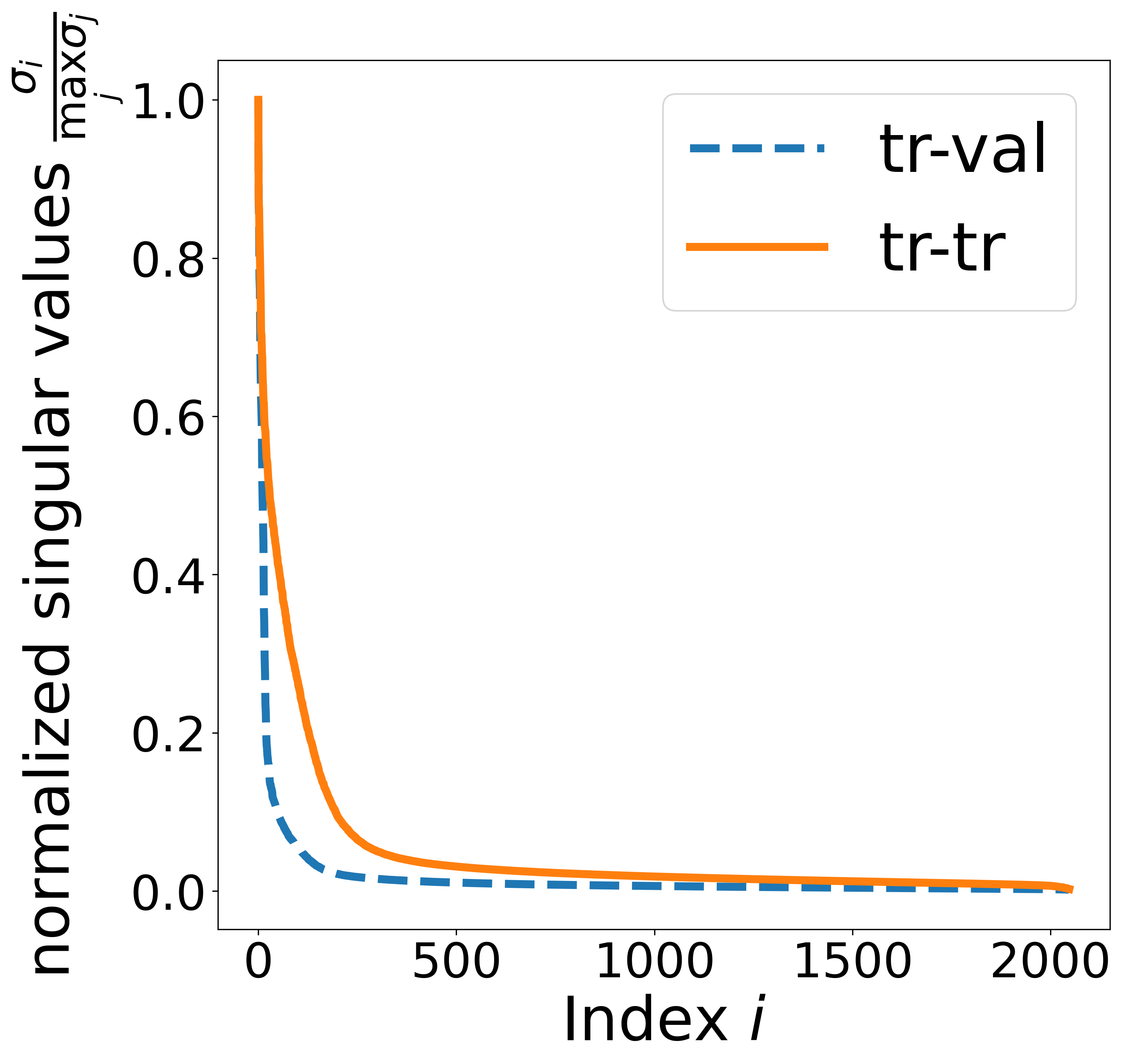
(a)

(b)

(c)

(d)

Figure 1: (a): Normalized singular values for tr-val versus tr-tr. Singular value decay for tr-val is faster, indicating that it has lower effective rank than tr-tr. (b,c): tSNE for tr-val and tr-tr representations respectively for inputs from 10 randomly selected test classes from Omniglot dataset. Dots with the same color correspond to points from the same class. We find that the tr-val representations are more clustered than the tr-tr representations. (d): tr-tr loss plotted in log scale versus training iteration for tr-val versus tr-tr runs at varying width factor $\ell$. This verifies that tr-tr models are indeed optimizing the loss that they were meant to minimize.

In this section we present experimental results that demonstrate the practical relevance of our theoretical results. For simulations we use the subspace learning meta-learning instance defined in Section 4.1 and verify that the tr-val objective is indeed superior to the tr-tr variant due to learning low-rank representation. We also perform experiments on the standard meta-learning benchmarks of Omniglot (Lake et al., 2015) and MiniImageNet (Vinyals et al., 2016) datasets, where we again find that representation learning benefits from tr-val splitting. Furthermore we show that iMAML Rajeswaran et al. (2019), a non-representation learning meta-learning algorithm, also benefits from tr-val splitting. iMAML was also used by Bai et al. (2020) to conclude the tr-tr is better than tr-val. We also perform a more detailed study of the learned representations on these benchmarks and find that while tr-val and tr-tr representations are almost equally expressive, tr-val representations have lower effective rank and thus have better few-shot performance. In Table 8 we verify that adding a Frobenius norm regularization on the representation with the tr-tr objective helps significantly, but is still slightly worse than tr-val splitting.

For our representation learning experiments, similar to ANIL algorithm (Raghu et al., 2020), we optimize the objective defined in Equation (5) that fixes the representation in the inner loop. Details of our first-order variant of ANIL (akin to first-order MAML (Finn et al., 2017)) are deferred to Section D.1; Algorithm 1 summarizes this RepLearn algorithm. Please refer to Section D for additional experiments.

Simulation: We simulate the meta-learning instance from Section 4.1 with $d=50$, $k=5$ and $\sigma=0.5$. The tr-tr models are trained by minimizing $\widehat{{\mathcal{L}}}^{\textmd{tr-tr}}_{\lambda,\textmd{rep}}(\cdot;n)$ with $n=16$ and tr-val models trained with $\widehat{{\mathcal{L}}}^{\textmd{tr-val}}_{\lambda,\textmd{rep}}(\cdot;(n_{1},n_{2}))$ with $n_{1}=8,n_{2}=8$. We tune $\bar{\lambda}$ for before meta-evaluation using validation tasks for each model. For meta-testing we evaluate with $\bar{n}_{1}\in\{5,15,25\}$ train samples per test task in Table 2. We find that the tr-val objective, trained with $\lambda=0$ as in Theorem 5.4, outperforms all tr-tr models, and does almost as well as the correct projection ${{{\bm{A}}}^{*}}{{{\bm{A}}}^{*}}^{\top}$. We notice that the tr-tr objective does not do as badly as ${{\bm{A}}}=I_{d}$, indicating that the training algorithm could have some useful inductive biases, but not enough. For the ${{\bm{A}}}\in\mathbb{R}^{50\times 50}$ learned using tr-val in the simulation experiment, the top $k=5$ singular values explain 95% of its total norm, thus implying that it is almost rank $k$. We also check the alignment of the top-$k$ singular directions of ${{\bm{A}}}$ with the optimal subspace and find the principle angle to be as small as $0.1^{\circ}$. For reference, the corresponding numbers for the best tr-tr learned ${{\bm{A}}}$ are $24\%$ and $5^{\circ}$ respectively.

RepLearn on Omniglot: We investigate the performance of tr-val and tr-tr objectives for representation learning on the Omniglot dataset for the 5-way 1-shot and 20-way 1-shot variants with a 4 layer convolution backbone as in Finn et al. (2017); results presented in Table 1. Following the same protocol as Bai et al. (2020), for meta-training we use $n=2N$ for tr-tr objective and $n_{1}=n_{2}=N$ for the tr-val objective for the $N$-way 1-shot task. For meta-testing we use $\bar{n}_{1}=N$. We find that tr-val outperforms tr-tr. Additional details are in Section D.

Capacity and tr-val versus tr-tr: We examine the performance gap between tr-val versus tr-tr as we increase the expressive power of the representation network. We use a baseline 4 hidden layer fully connected network (FCN) inspired by Rajeswaran et al. (2019), but with $64\ell$ nodes at all 4 layers for different values of $\ell\in\{1,4,8,16,32\}$. Using FCNs gets rid of inductive biases of CNNs and helps distill the role of data splitting better. The models are trained using tr-tr and tr-val representation learning objectives on the Omniglot 5-way 1-shot dataset; results presented in Table 3.. We find that increasing width tends to slightly improve the performance of tr-val models but hurts the performance of tr-tr models, thus increasing the gap between tr-val and tr-tr. Additionally, we note that the tr-tr model succeeds in minimizing the tr-tr loss ${\mathcal{L}}^{\textmd{tr-tr}}$ as evident in Figure 1(d). Thus its bad performance on meta-learning is not an optimization issue, but can be attributed to learning overly expressive representations due to lack of explicit regularization, as predicted by Theorem 5.1. This demonstrates that the tr-val objective is more robust to choice of model architecture.

Table 3: Accuracies in % of representations parameterized by fully connected networks of varying widths on Omniglot 5-way 1-shot meta-testing and on a supervised dataset that is constructed using the 413 test classes from Omniglot. Representations trained using tr-val objective consistently outperforms those learned using tr-tr objective, and the gap increases as width increases.

width $=$	Omniglot 5-way 1-shot		Supervised 413-way
$64^{*}\ell$	tr-val	tr-tr	tr-val	tr-tr
$\ell=1$	87.8 $\pm$ 1.1	80.6 $\pm$ 1.4	87.4	73.4
$\ell=4$	90.8 $\pm$ 1.0	77.8 $\pm$ 1.4	100.0	100.0
$\ell=8$	91.6 $\pm$ 1.0	73.9 $\pm$ 1.5	100.0	100.0
$\ell=16$	91.7 $\pm$ 0.9	70.6 $\pm$ 1.6	100.0	100.0
$\ell=32$	91.6 $\pm$ 1.0	67.8 $\pm$ 1.6	100.0	100.0

Low-rankness and expressivity: We investigate the representations from the trained FCNs with $\ell=32$. To ascertain expressivity of representations, we combine all data from the test classes of Omniglot to produce a supervised learning dataset with 413 classes. We measure expressivity of representations by evaluating its linear classification performance on the 413-way supervised task; results in Table 3. We find that the tr-val representations do at least as well as tr-tr ones and thus are expressive enough. To compare the effective ranks, we plot the normalized singular values of both sets of representations in Figure 1(a) and find that the tr-val representations have a steeper drop in singular values than the tr-tr representations, thus confirming their lower effective rank. t-SNE plots (Figure 1(b) and Figure 1(c)) on the tr-val and tr-tr representations for data points from 10 randomly selected classes suggest that tr-val representations are better clustered than the tr-tr representations.

iMAML on Omniglot: We go beyond representation learning and consider a meta-learning method iMAML (Rajeswaran et al., 2019) that updates all parameters in the inner loop. We modify the authors code to implement a tr-tr version and we investigate the performance of tr-val and tr-tr objectives on the Omniglot dataset for both 5-way 1-shot and 20-way 1-shot settings in Table 1. We find that tr-val outperforms tr-tr again, this time by a significant margin. We do not tune hyper-parameters for tr-val and just use the defaults, but for tr-tr we tune them to give it an edge.

RepLearn on MiniImageNet: We performs similar experiments on MiniImageNet using a standard CNN backbone with 32, 64, 128, and 128 filters, respectively. Table 5 shows again that RepLearn with tr-val splitting is much better than tr-tr on 5-way 1-shot and 5-way 5-shot settings, similar to the findings with Omniglot. We also perform the capacity experiment by increasing the number of filters by a factor $\ell$; the convolutional layers contain $32\ell$, $64\ell$, $128\ell$, and $128\ell$ output filters, respectively. Results in Table 4 suggest that increasing the network capacity improves the performance of tr-val representations, but slightly hurts tr-tr performance, just like the findings for Omniglot dataset with fully-connected networks. The drop might be lower here due to a CNN being used instead of fully connected network in Table 3. Thus the tr-val method is more robust to architecture choice/capacity and datasets.

Table 4: Accuracies in % of representations parameterized by CNN networks with varying number of filters on MiniImageNet. Representations trained using tr-val objective consistently outperforms those learned using tr-tr objective; gap increases as width increases.

capacity $=$	MiniImageNet 5-way 1-shot
$num\_filters^{*}\ell$	tr-val	tr-tr
$\ell=0.5$	46.66 $\pm$ 1.69	26.25 $\pm$ 1.45
$\ell=1$	48.44 $\pm$ 1.62	26.81 $\pm$ 1.44
$\ell=4$	52.22 $\pm$ 1.68.	24.66 $\pm$ 1.26
$\ell=8$	52.25 $\pm$ 1.71	25.28 $\pm$ 1.37

Table 5: Tr-val v/s tr-tr meta-test accuracies in % for a CNN model trained with RepLearn on MiniImageNet 5-way 1-shot and 5-way 5-shot for varying values of the regularization parameter, $\lambda$.

	5-way 1-shot	5-way 5-shot
$\lambda=$ 0.0 tr-val	46.16 $\pm$ 1.67	65.36 $\pm$ 0.91
$\lambda=$ 0.0 tr-tr	25.53 $\pm$ 1.43	33.49 $\pm$ 0.82
$\lambda=$ 0.1 tr-tr	24.69 $\pm$ 1.32	34.91 $\pm$ 0.85
$\lambda=$ 1.0 tr-tr	25.88 $\pm$ 1.45	40.19 $\pm$ 1.12

7 Discussions and Future Work

We study the implicit regularization effect of the practical design choice of train-validation splitting popular in meta-learning, and show that it encourages learning low-rank but expressive enough representations. This is contrasted with the non-splitting variant that is shown to fail without explicit regularization. Both of these claims are justified theoretically for linear representation learning and experimentally for standard meta-learning benchmarks. Train-validation splitting provides a new mechanism for sample efficiency through implicit regularization in the objective, as opposed to explicit regularization and implicit bias of training algorithm, as discussed in Section 5.3. We show learning of exact low rank representations in our setting as opposed to approximate low-rankness observed in practice. Relaxing assumptions of Gaussianity, common input distribution across tasks and linearity of representations might explain the observed effective low-rankness. Finally an interesting problem is to get the best of all worlds, data efficiency from tr-tr style objective, explicit regularization and the implicit low rank regularization from tr-val splitting in a principled way. Identifying and understanding other training paradigms that intrinsically use data efficiently, even without explicit regularization is also an interesting direction.

Acknowlegments: We thank Mikhail Khodak for comments on an earlier draft of the paper. Nikunj Saunshi, Arushi Gupta and Wei Hu are supported by NSF, ONR, Simons Foundation, Amazon Research, DARPA and SRC.

Appendix A Appendix Overview

The Appendix is structured as follows

• Section B proves the result for linear representation learning with the tr-tr objective, Theorem 5.1, that shows that “bad” full rank solutions exist arbitrarily close to the optimal value of the tr-tr objective ${\mathcal{L}}^{\textmd{tr-tr}}_{\lambda,\textmd{rep}}$. The proof works by arguing that smaller values of $\lambda$ are desirable for the tr-tr objective, and this can be simulated by effectively making the norm of the representation layer very high. Furthermore a higher rank representation is preferable over lower rank ones to fit the noise in the labels in the training data better.

• Section C proves the main result for linear representation learning with tr-val objective, Theorem 5.4, that proves that the optimal solutions to the tr-val objective ${\mathcal{L}}^{\textmd{tr-val}}_{\lambda,\textmd{rep}}({{\bm{A}}};(n_{1},n_{2}))$ for most $n_{1}$ and $\sigma$ will be low-rank representations that are also expressive enough. The result is also extended to solutions that are $\tau$-optimal in the ${\mathcal{L}}^{\textmd{tr-val}}_{\lambda,\textmd{rep}}$ objective for a small enough $\tau$. The crux of the proof for this result is in Theorem C.1 that provides a closed form expression for the tr-val objective that disentangles the expressivity and the low-rankness of the representation.

• Section D presents additional experimental details and results, including results for the MiniImageNet dataset.

Appendix B More on Train-Train split

B.1 Proof of main result

Theorem 5.1.

For every $\lambda,n>0$, for every $\tau>0$, there exists a “bad” representation layer ${{\bm{A}}}_{\textmd{bad}}\in\mathbb{R}^{d\times d}$ that satisfies ${\mathcal{L}}^{\textmd{tr-tr}}_{\lambda,\textmd{rep}}({{\bm{A}}}_{\textmd{bad}};n)\leq\inf\limits_{{{\bm{A}}}\in\mathbb{R}^{d\times d}}{\mathcal{L}}^{\textmd{tr-tr}}_{\lambda,\textmd{rep}}({{\bm{A}}};n)+\tau$, but has the following lower bound on meta-testing loss

$$\inf_{\bar{\lambda}>0} {\mathcal{L}}^{\textmd{test}}_{\bar{\lambda},\textmd{rep}}({{\bm{A}}}_{\textmd{bad}};\bar{n}_{1})\geq\sigma^{2}+\min\left\{1-\frac{\bar{n}_{1}}{d(1+\sigma^{2})},\frac{d\sigma^{2}}{(\bar{n}_{1}+d\sigma^{2})}\right\}$$

Proof.

For most of the proof, we will leave out the $n$ in the expression for ${\mathcal{L}}^{\textmd{tr-tr}}_{\lambda,\textmd{rep}}$, i.e. we will denote the tr-tr loss as ${\mathcal{L}}^{\textmd{tr-tr}}_{\lambda,\textmd{rep}}({{\bm{A}}})$. We prove this result by using Lemma 5.2 first, and later prove this lemma.

Lemma 5.2.

For every $\lambda>0$ and ${{\bm{A}}}\in\mathbb{R}^{d\times d}$ with rank $r$,

$${\mathcal{L}}^{\textmd{tr-tr}}_{\lambda,\textmd{rep}}({{\bm{A}}};n)\geq\lim_{\kappa\rightarrow\infty}{\mathcal{L}}^{\textmd{tr-tr}}_{\lambda,\textmd{rep}}(\kappa {{\bm{A}}};n)\geq\sigma^{2}\frac{(n-r)_{+}}{n}$$

$$\text{ \& }~{}\lim_{\kappa\rightarrow\infty}{\mathcal{L}}^{\textmd{tr-tr}}_{\lambda,\textmd{rep}}(\kappa{\bm{I}}_{d};n) =\sigma^{2}\frac{(n-d)_{+}}{n}$$

This tells us that for any matrix ${{\bm{A}}}$, ${\mathcal{L}}^{\textmd{tr-tr}}_{\lambda,\textmd{rep}}({{\bm{A}}})\geq\sigma^{2}\frac{(n-\textrm{rank}({{\bm{A}}}))_{+}}{n}\geq\sigma^{2}\frac{(n-d)_{+}}{n}$. Also the lower bound of $\sigma^{2}\frac{(n-d)_{+}}{n}$ can be achieved by $\kappa{\bm{I}}_{d}$ in the limit of $\kappa\rightarrow\infty$, thus $\sigma^{2}\frac{(n-d)_{+}}{n}=\inf_{{{\bm{A}}}\in\mathbb{R}^{d\times d}}{\mathcal{L}}^{\textmd{tr-tr}}_{\lambda,\textmd{rep}}({{\bm{A}}})$. Also since $\lim_{\kappa\rightarrow\infty}\kappa{\bm{I}}_{d}=\sigma^{2}\frac{(n-d)_{+}}{n}=\inf_{{{\bm{A}}}\in\mathbb{R}^{d\times d}}{\mathcal{L}}^{\textmd{tr-tr}}_{\lambda,\textmd{rep}}({{\bm{A}}})$, for a large enough $\kappa=\kappa(\tau)$, ${\mathcal{L}}^{\textmd{tr-tr}}_{\lambda,\textmd{rep}}(\kappa(\tau){\bm{I}}_{d})$ can be made lesser than $\inf_{{{\bm{A}}}\in\mathbb{R}^{d\times d}}{\mathcal{L}}^{\textmd{tr-tr}}_{\lambda,\textmd{rep}}({{\bm{A}}})+\tau$. Thus we pick ${{\bm{A}}}_{\textmd{bad}}=\kappa(\tau){\bm{I}}_{d}$. With this choice, the new task is essentially linear regression in $d$-dimension with isotropic Gaussians.

To show that ${{\bm{A}}}_{\textmd{bad}}$ is indeed bad, we will use the lower bound for ridge regression on isotropic Gaussian linear regression from Theorem 4.2(a) in Saunshi et al. [2020]. They show that the excess risk for ${\bm{I}}_{d}$ (and thus $\kappa(\tau){\bm{I}}_{d}$), regardless of the choice of regularizer $\bar{\lambda}$, for a new task $\rho_{{{\bm{v}}}}$ will be lower bounded by

$$\inf_{\bar{\lambda}>0}\mathop{\mathbb{E}}\limits_{S\sim\rho_{{{\bm{v}}}}^{\bar{n}_{1}}}\left[\|{{\bm{A}}}{{\bm{w}}}_{\bar{\lambda}}({{\bm{A}}};S)-{{\bm{v}}}\|^{2}\right] \geq\begin{cases}\frac{d\|{{\bm{v}}}\|^{2}\sigma^{2}}{\bar{n}_{1}\|{{\bm{v}}}\|+\sigma^{2}d}&\text{if }\bar{n}_{1}\geq d\\ &\\ \frac{\bar{n}_{1}}{d}\frac{\|{{\bm{v}}}\|^{2}\sigma^{2}}{\|{{\bm{v}}}\|+\sigma^{2}}+\frac{d-\bar{n}_{1}}{d}\|{{\bm{v}}}\|^{2}&\text{if }\bar{n}_{1}<d\\ \end{cases}$$

Their proof can be easily modified to replace $\|{{\bm{v}}}\|^{2}$ with $\mathop{\mathbb{E}}\limits_{{{\bm{v}}}\sim\bar{\mu}}\|{{\bm{v}}}\|^{2}$. The lower bound can be simplified for the the $\bar{n}_{1}<d$ case to $\frac{\bar{n}_{1}}{d}\frac{\|{{\bm{v}}}\|^{2}\sigma^{2}}{\|{{\bm{v}}}\|+\sigma^{2}}+\frac{d-\bar{n}_{1}}{d}\|{{\bm{v}}}\|^{2}=\|{{\bm{v}}}\|^{2}-\frac{\bar{n}_{1}}{d}\frac{\|{{\bm{v}}}\|^{2}}{\|{{\bm{v}}}\|^{2}+\sigma^{2}}$. Plugging in $\|{{\bm{v}}}\|=1$ completes the proof. ∎

We now prove the lemma

Lemma 5.2.

For every $\lambda>0$ and ${{\bm{A}}}\in\mathbb{R}^{d\times d}$ with rank $r$,

$${\mathcal{L}}^{\textmd{tr-tr}}_{\lambda,\textmd{rep}}({{\bm{A}}};n)\geq\lim_{\kappa\rightarrow\infty}{\mathcal{L}}^{\textmd{tr-tr}}_{\lambda,\textmd{rep}}(\kappa {{\bm{A}}};n)\geq\sigma^{2}\frac{(n-r)_{+}}{n}$$

$$\text{ \& }~{}\lim_{\kappa\rightarrow\infty}{\mathcal{L}}^{\textmd{tr-tr}}_{\lambda,\textmd{rep}}(\kappa{\bm{I}}_{d};n) =\sigma^{2}\frac{(n-d)_{+}}{n}$$

Proof.

We first prove that having $\lambda=0$ will lead to the smallest loss ${\mathcal{L}}^{\textmd{tr-tr}}_{\lambda,\textmd{rep}}({{\bm{A}}})$ for every ${{\bm{A}}}$. We then observe that $\lambda=0$ can be simulated by increasing the norm of ${{\bm{A}}}$. These claims mathematically mean that, (a) ${\mathcal{L}}^{\textmd{tr-tr}}_{\lambda,\textmd{rep}}({{\bm{A}}})\geq{\mathcal{L}}^{\textmd{tr-tr}}_{\lambda^{\prime},\textmd{rep}}({{\bm{A}}})$ whenever $\lambda\geq\lambda^{\prime})$ and (b) ${\mathcal{L}}^{\textmd{tr-tr}}_{\lambda,\textmd{rep}}(\kappa{{\bm{A}}})={\mathcal{L}}^{\textmd{tr-tr}}_{\frac{\lambda}{\kappa^{2}},\textmd{rep}}({{\bm{A}}})$. This will give us that $\lim_{\kappa\rightarrow\infty}{\mathcal{L}}^{\textmd{tr-tr}}_{\lambda,\textmd{rep}}(\kappa{{\bm{A}}})=\lim_{\lambda\rightarrow 0}{\mathcal{L}}^{\textmd{tr-tr}}_{0,\textmd{rep}}(\kappa{{\bm{A}}})\geq{\mathcal{L}}^{\textmd{tr-tr}}_{\lambda,\textmd{rep}}({{\bm{A}}})$. Intuitively, ${\mathcal{L}}^{\textmd{tr-tr}}_{\lambda,\textmd{rep}}$ is trying to learn a linear classifier on top of data that is linear transformed by ${{\bm{A}}}$ with the goal of fitting the same data well.

Lemma B.1.

For any representation layer ${{\bm{A}}}\in\mathbb{R}^{d\times d}$ and $\lambda>0$, we have the following

$$\lim_{\kappa\rightarrow\infty}{\mathcal{L}}^{\textmd{tr-tr}}_{\lambda,\textmd{rep}}(\kappa{{\bm{A}}})=\lim_{\lambda\rightarrow 0}{\mathcal{L}}^{\textmd{tr-tr}}_{\lambda,\textmd{rep}}({{\bm{A}}})\leq{\mathcal{L}}^{\textmd{tr-tr}}_{\lambda,\textmd{rep}}({{\bm{A}}})$$

Fitting the data is better when there is less restriction on the norm of the classifier, which in this case means when $\lambda$ is smaller. Furthermore, increasing the norm of the representation layer ${{\bm{A}}}$ effectively reduces the impact the regularizer will have. We first prove this lemma later, first we use it to prove Lemma 5.2 that shows that the loss for low rank matrices will be high.

Lemma B.1 already shows that ${\mathcal{L}}^{\textmd{tr-tr}}_{\lambda,\textmd{rep}}({{\bm{A}}};n)\geq\lim_{\kappa\rightarrow\infty}{\mathcal{L}}^{\textmd{tr-tr}}_{\lambda,\textmd{rep}}(\kappa{{\bm{A}}};n)$. Also using Lemma B.1, we can replace $\lim_{\kappa\rightarrow\infty}{\mathcal{L}}^{\textmd{tr-tr}}_{\lambda,\textmd{rep}}(\kappa{{\bm{A}}})$ with $\lim_{\lambda\rightarrow 0}{\mathcal{L}}^{\textmd{tr-tr}}_{\lambda,\textmd{rep}}({{\bm{A}}})$. Using Equation (9) and from central limit theorem, we have

$${\mathcal{L}}^{\textmd{tr-tr}}_{\lambda,\textmd{rep}}({{\bm{A}}})=\lim_{T\rightarrow\infty}\widehat{{\mathcal{L}}}^{\textmd{tr-tr}}({{\bm{A}}}) =\mathop{\mathbb{E}}\limits_{\rho_{{{\bm{v}}}}\sim\mu}\left[\mathop{\mathbb{E}}\limits_{S\sim\rho_{{{\bm{v}}}}^{n}}\left[\frac{1}{n}\|{\bm{X}}{{\bm{A}}}{{\bm{w}}}_{\lambda}({{\bm{A}}};S)-{\bm{Y}}\|^{2}\right]\right]$$ (14)

$$=\mathop{\mathbb{E}}\limits_{{{\bm{v}}}\sim{\mathcal{N}}({\bm{0}}_{d},{{{\bm{A}}}^{*}}{{{\bm{A}}}^{*}}^{\top})}\left[\mathop{\mathbb{E}}\limits_{S\sim\rho_{{{\bm{v}}}}^{n}}\left[\frac{1}{n}\|{\bm{X}}{{\bm{A}}}{{\bm{w}}}_{\lambda}({{\bm{A}}};S)-{\bm{Y}}\|^{2}\right]\right]$$ (15)

This is because $\widehat{{\mathcal{L}}}^{\textmd{tr-tr}}_{\lambda,\textmd{rep}}$ is an average loss for $T$ train tasks, and the limit when $T\rightarrow\infty$ it converges to the expectation over the task distribution $\mu$. We first observe that $S\sim\rho_{{{\bm{v}}}}$ is equivalent to sampling ${\bm{X}}\sim{\mathcal{N}}({\bm{0}}_{d},{\bm{I}}_{d})$, $\bm{\eta}\sim{\mathcal{N}}({\bm{0}}_{n},\sigma^{2}I_{n})$ which gives us ${\bm{Y}}={\bm{X}}{{\bm{v}}}+\bm{\eta}$, where ${\bm{X}}\in\mathbb{R}^{n\times d},\bm{\eta}\in\mathbb{R}^{n},{\bm{Y}}\in\mathbb{R}^{n}$. Using the definition of ${{\bm{w}}}_{\lambda}({{\bm{A}}};S)$ from Equation (8) the standard KKT condition for linear regression, we can write a closed form solution for

$${{\bm{w}}}_{\lambda}({{\bm{A}}};S) =\operatorname*{arg\,min}_{{{\bm{w}}}\in\mathbb{R}^{d}}\frac{1}{n}\|{\bm{X}}{{\bm{A}}}{{\bm{w}}}-{\bm{Y}}\|^{2}+\lambda\|{{\bm{w}}}\|^{2}=\left(\frac{{{\bm{A}}}^{\top}{\bm{X}}^{\top}{\bm{X}}{{\bm{A}}}}{n}+\lambda{\bm{I}}_{d}\right)^{-1}\frac{{{\bm{A}}}^{\top}{\bm{X}}^{\top}}{n}{\bm{Y}}$$ (16)

$$\lim_{\lambda\rightarrow 0}{{\bm{w}}}_{\lambda}({{\bm{A}}};S) =\left(\frac{{{\bm{A}}}^{\top}{\bm{X}}^{\top}{\bm{X}}{{\bm{A}}}}{n}\right)^{\dagger}\frac{{{\bm{A}}}^{\top}{\bm{X}}^{\top}}{n}{\bm{Y}}$$ (17)

where the last step is folklore that the limit of ridge regression as regularization coefficient goes to 0 is the minimum $\ell_{2}$-norm linear regression solution. Plugging this into Equation (20) and taking the limit

$$\lim_{\lambda\rightarrow 0}{\mathcal{L}}^{\textmd{tr-tr}}_{\lambda,\textmd{rep}}({{\bm{A}}}) =\mathop{\mathbb{E}}\limits_{{{\bm{v}}},S}\left[\frac{1}{n}\left\|{\bm{X}}{{\bm{A}}}\left(\lim_{\lambda\rightarrow 0}{{\bm{w}}}_{\lambda}({{\bm{A}}};S)\right)-{\bm{Y}}\right\|^{2}\right]$$

$$=\mathop{\mathbb{E}}\limits_{{{\bm{v}}},S}\left[\frac{1}{n}\left\|\left({\bm{X}}{{\bm{A}}}\left(\frac{{{\bm{A}}}^{\top}{\bm{X}}^{\top}{\bm{X}}{{\bm{A}}}}{n}\right)^{\dagger}\frac{{{\bm{A}}}^{\top}{\bm{X}}^{\top}}{n}-I_{n}\right){\bm{Y}}\right\|^{2}\right]$$

$$=\frac{1}{n}\mathop{\mathbb{E}}\limits_{{{\bm{v}}},S}\left[\left\|P^{\perp}_{{\bm{X}}{{\bm{A}}}}{\bm{Y}}\right\|^{2}\right]$$

where for any matrix ${\bm{B}}\in\mathbb{R}^{n\times d}$, we denote $P_{{\bm{B}}}\in\mathbb{R}^{n\times n}={\bm{B}}{\bm{B}}^{\dagger}$ to denote the projection matrix onto the span of columns of ${\bm{B}}$, and $P^{\perp}_{{\bm{B}}}=I_{n}-P_{{\bm{B}}}$ is the projection matrix onto the orthogona subspace. Note that if $\textrm{rank}({\bm{B}})=n$, then $P_{{\bm{B}}}=I_{n}$ and $P^{\perp}_{{\bm{B}}}=0$. Thus the error incurred is the amount of the label ${\bm{Y}}$ that the representation ${\bm{X}}{{\bm{A}}}$ cannot predict linearly. We further decompose this

$$\lim_{\lambda\rightarrow 0}{\mathcal{L}}^{\textmd{tr-tr}}_{\lambda,\textmd{rep}}({{\bm{A}}}) =\frac{1}{n}\mathop{\mathbb{E}}\limits_{{{\bm{v}}},S}\left[\left\|P^{\perp}_{{\bm{X}}{{\bm{A}}}}{\bm{Y}}\right\|^{2}\right]=\frac{1}{n}\mathop{\mathbb{E}}\limits_{{{\bm{v}}},S}\left[\left\|P^{\perp}_{{\bm{X}}{{\bm{A}}}}{\bm{X}}{{\bm{v}}}+P^{\perp}_{{\bm{X}}{{\bm{A}}}}\bm{\eta}\right\|^{2}\right]$$

$$=\underbrace{\frac{1}{n}\mathop{\mathbb{E}}\limits_{{{\bm{v}}},S}\left[\left\|P^{\perp}_{{\bm{X}}{{\bm{A}}}}{\bm{X}}{{\bm{v}}}\right\|^{2}\right]}_{\text{fitting signal}}+\underbrace{\frac{1}{n}\mathop{\mathbb{E}}\limits_{{{\bm{v}}},S}\left[\left\|P^{\perp}_{{\bm{X}}{{\bm{A}}}}\bm{\eta}\right\|^{2}\right]}_{\text{fitting noise}}+\underbrace{\frac{2}{n}\mathop{\mathbb{E}}\limits_{{{\bm{v}}},S}\left[\bm{\eta}^{\top}P^{\perp}_{{\bm{X}}{{\bm{A}}}}{\bm{X}}{{\bm{v}}}\right]}_{\text{cross term}}$$ (18)

$$=\frac{1}{n}\mathop{\mathbb{E}}\limits_{S}\mathop{\mathbb{E}}\limits_{{{\bm{v}}}\sim{\mathcal{N}}({\bm{0}}_{d},{{{\bm{A}}}^{*}}{{{\bm{A}}}^{*}}^{\top})}\left[\left\|P^{\perp}_{{\bm{X}}{{\bm{A}}}}{\bm{X}}{{\bm{v}}}\right\|^{2}\right]+\mathop{\mathbb{E}}\limits_{S}\frac{1}{n}\textrm{tr}\left(P^{\perp}_{{\bm{X}}{{\bm{A}}}}\mathop{\mathbb{E}}\limits_{\bm{\eta}}\left[\bm{\eta}\bm{\eta}^{\top}\right]P^{\perp}_{{\bm{X}}{{\bm{A}}}}\right)$$

$$=\underbrace{\frac{1}{n}\mathop{\mathbb{E}}\limits_{S}\left[\left\|P^{\perp}_{{\bm{X}}{{\bm{A}}}}{\bm{X}}{{{\bm{A}}}^{*}}\right\|^{2}\right]}_{\alpha({{\bm{A}}})}+\underbrace{\mathop{\mathbb{E}}\limits_{S}\frac{\sigma^{2}}{n}\textrm{tr}\left(P^{\perp}_{{\bm{X}}{{\bm{A}}}}\right)}_{\beta({{\bm{A}}})}$$ (19)

We first note, due to independence of $\bm{\eta}$ and ${\bm{X}}$ that the cross term in Equation (18) is 0 in expectation. Using the distributions for ${{\bm{v}}}\sim{\mathcal{N}}({\bm{0}}_{d},{{{\bm{A}}}^{*}}{{{\bm{A}}}^{*}}^{\top})$ and $\bm{\eta}\sim{\mathcal{N}}({\bm{0}}_{n},\sigma^{2}I_{n})$, we get the final expressions Firstly, we note that $\alpha({{\bm{A}}})\geq 0$ for every ${{\bm{A}}}$, and a sufficient condition for $\alpha({{\bm{A}}})=0$ is that ${{{\bm{A}}}^{*}}$ lies in the span of ${{\bm{A}}}$, i.e. $P^{\perp}_{{{\bm{A}}}}{{{\bm{A}}}^{*}}=0$. More importantly, it is clear that $\alpha({\bm{I}}_{d})=0$. Next we look at the $\beta({{\bm{A}}})$ term which is proportional to the trace of $P^{\perp}_{{\bm{X}}{{\bm{A}}}}$ which, for a projection matrix, is also equal to the rank of the matrix. Note that since the rank of ${\bm{X}}{{\bm{A}}}\in\mathbb{R}^{d\times n}$ is at most $\min\{n,d\}$. Thus we get

$$\beta({{\bm{A}}})=\sigma^{2}\frac{\textrm{rank}(P^{\perp}_{{\bm{X}}{{\bm{A}}}})}{n}=\sigma^{2}\frac{(n-\textrm{rank}(P^{\perp}_{{\bm{X}}{{\bm{A}}}}))}{n}\geq\sigma^{2}\frac{(n-\textrm{rank}({{\bm{A}}}))_{+}}{n}$$

where $(x)_{+}=\mathds{1}_{x\geq 0}x$. This along with $\alpha({{\bm{A}}})\geq 0$ proves the first part of the result. For the second part $\alpha({\bm{I}}_{d})=0$ along with noticing that $\textrm{tr}(P^{\perp}_{{\bm{X}}{\bm{I}}_{d}})=n-\textrm{rank}({\bm{X}})=n-\min\{n,d\}$ since a Gaussian matrix is full rank with measure 1, thus giving us $\beta({\bm{I}}_{d})=\sigma^{2}\frac{(n-d)_{+}}{n}$ and completing the proof. ∎

Thus Lemma 5.2 shows that $\lim_{\kappa\rightarrow\infty}{\mathcal{L}}^{\textmd{tr-tr}}_{\lambda,\textmd{rep}}(\kappa{\bm{I}}_{d})=\inf_{{{\bm{A}}}}{\mathcal{L}}^{\textmd{tr-tr}}_{\lambda,\textmd{rep}}({{\bm{A}}})$ and so picking a large enough $\kappa(\tau)$ can always give us ${\mathcal{L}}^{\textmd{tr-tr}}_{\lambda,\textmd{rep}}(\kappa(\tau){\bm{I}}_{d})\leq\inf_{{{\bm{A}}}}{\mathcal{L}}^{\textmd{tr-tr}}_{\lambda,\textmd{rep}}({{\bm{A}}})+\tau$ which completes the proof of Theorem 5.1. The only thing left to prove is Lemma B.1 which we do below

Proof of Lemma B.1.

Using Equation (16) we get the following expression for ${\mathcal{L}}^{\textmd{tr-tr}}_{\lambda,\textmd{rep}}$

$${\mathcal{L}}^{\textmd{tr-tr}}_{\lambda,\textmd{rep}}({{\bm{A}}}) =\mathop{\mathbb{E}}\limits_{{{\bm{v}}},S}\left[\frac{1}{n}\left\|{\bm{X}}{{\bm{A}}}{{\bm{w}}}_{\lambda}({{\bm{A}}};S)-{\bm{Y}}\right\|^{2}\right]$$

$$=\mathop{\mathbb{E}}\limits_{{{\bm{v}}},S}\left[\frac{1}{n}\left\|\left({\bm{X}}{{\bm{A}}}\left(\frac{{{\bm{A}}}^{\top}{\bm{X}}^{\top}{\bm{X}}{{\bm{A}}}}{n}+\lambda{\bm{I}}_{d}\right)^{-1}\frac{{{\bm{A}}}^{\top}{\bm{X}}^{\top}}{n}-I_{n}\right){\bm{Y}}\right\|^{2}\right]$$ (20)

From this we get

$${\mathcal{L}}^{\textmd{tr-tr}}_{\lambda,\textmd{rep}}(\kappa{{\bm{A}}}) =\mathop{\mathbb{E}}\limits_{{{\bm{v}}},S}\left[\frac{1}{n}\left\|\left(\kappa{\bm{X}}{{\bm{A}}}\left(\frac{\kappa^{2}{{\bm{A}}}^{\top}{\bm{X}}^{\top}{\bm{X}}{{\bm{A}}}}{n}+\lambda{\bm{I}}_{d}\right)^{-1}\frac{\kappa{{\bm{A}}}^{\top}{\bm{X}}^{\top}}{n}-I_{n}\right){\bm{Y}}\right\|^{2}\right]$$

$$=\mathop{\mathbb{E}}\limits_{{{\bm{v}}},S}\left[\frac{1}{n}\left\|\left({\bm{X}}{{\bm{A}}}\left(\frac{{{\bm{A}}}^{\top}{\bm{X}}^{\top}{\bm{X}}{{\bm{A}}}}{n}+\frac{\lambda}{\kappa^{2}}{\bm{I}}_{d}\right)^{-1}\frac{{{\bm{A}}}^{\top}{\bm{X}}^{\top}}{n}-I_{n}\right){\bm{Y}}\right\|^{2}\right]$$

$$={\mathcal{L}}^{\textmd{tr-tr}}_{\frac{\lambda}{\kappa^{2}},\textmd{rep}}({{\bm{A}}})$$

Thus $\lim\limits_{\kappa\rightarrow\infty}{\mathcal{L}}^{\textmd{tr-tr}}_{\lambda,\textmd{rep}}(\kappa{{\bm{A}}})=\lim\limits_{\kappa\rightarrow\infty}{\mathcal{L}}^{\textmd{tr-tr}}_{\frac{\lambda}{\kappa^{2}},\textmd{rep}}({{\bm{A}}})=\lim\limits_{\lambda\rightarrow 0}{\mathcal{L}}^{\textmd{tr-tr}}_{\lambda,\textmd{rep}}({{\bm{A}}})$. Note that we have used the fact that ${\mathcal{L}}^{\textmd{tr-tr}}_{\lambda,\textmd{rep}}$ is continuous in $\lambda$ for $\lambda>0$. To prove the remaining result, i.e. $\lim\limits_{\lambda\rightarrow 0}{\mathcal{L}}^{\textmd{tr-tr}}_{\lambda,\textmd{rep}}({{\bm{A}}})\leq{\mathcal{L}}^{\textmd{tr-tr}}_{\lambda,\textmd{rep}}({{\bm{A}}})$, we just need to prove that ${\mathcal{L}}^{\textmd{tr-tr}}_{\lambda,\textmd{rep}}({{\bm{A}}})$ is a increasing function of $\lambda$. Suppose $\frac{{\bm{X}}{{\bm{A}}}}{\sqrt{n}}={\bm{U}}_{{\bm{X}}}{\bm{S}}_{{\bm{X}}}{\bm{V}}_{{\bm{X}}}^{\top}$ is the singular value decomposition. For any $\lambda^{\prime}<\lambda$, we can rewrite ${\mathcal{L}}^{\textmd{tr-tr}}_{\lambda,\textmd{rep}}({{\bm{A}}})$ from Equation (20) as follows

$${\mathcal{L}}^{\textmd{tr-tr}}_{\lambda,\textmd{rep}}({{\bm{A}}}) =\mathop{\mathbb{E}}\limits_{{{\bm{v}}},S}\left[\frac{1}{n}\left\|\left({\bm{X}}{{\bm{A}}}\left(\frac{{{\bm{A}}}^{\top}{\bm{X}}^{\top}{\bm{X}}{{\bm{A}}}}{n}+\lambda{\bm{I}}_{d}\right)^{-1}\frac{{{\bm{A}}}^{\top}{\bm{X}}^{\top}}{n}-I_{n}\right){\bm{Y}}\right\|^{2}\right]$$

$$=\mathop{\mathbb{E}}\limits_{{{\bm{v}}},S}\left[\frac{1}{n}\left\|\left({\bm{V}}_{{\bm{X}}}{\bm{S}}_{{\bm{X}}}{\bm{U}}_{{\bm{X}}}^{\top}\left({\bm{U}}_{{\bm{X}}}{\bm{S}}_{{\bm{X}}}{\bm{V}}_{{\bm{X}}}^{\top}{\bm{V}}_{{\bm{X}}}{\bm{S}}_{{\bm{X}}}{\bm{U}}_{{\bm{X}}}^{\top}+\lambda{\bm{I}}_{d}\right)^{-1}{\bm{U}}_{{\bm{X}}}{\bm{S}}_{{\bm{X}}}{\bm{V}}_{{\bm{X}}}^{\top}-I_{n}\right){\bm{Y}}\right\|^{2}\right]$$

$$=\mathop{\mathbb{E}}\limits_{{{\bm{v}}},S}\left[\frac{1}{n}\left\|{\bm{V}}_{{\bm{X}}}\left({\bm{S}}_{{\bm{X}}}\left({\bm{S}}^{2}_{{\bm{X}}}+\lambda{\bm{I}}_{d}\right)^{-1}{\bm{S}}_{{\bm{X}}}-I_{n}\right){\bm{V}}_{{\bm{X}}}^{\top}{\bm{Y}}\right\|^{2}\right]$$

$$=\mathop{\mathbb{E}}\limits_{{{\bm{v}}},S}\left[\frac{1}{n}\sum_{i=1}^{d}\left[\left(\frac{{\bm{S}}_{{\bm{X}}}[i]^{2}}{\lambda+{\bm{S}}_{{\bm{X}}}[i]^{2}}-1\right)^{2}{\bm{V}}_{{\bm{X}}}^{\top}{\bm{Y}}[i]^{2}\right]\right]$$

$$=\mathop{\mathbb{E}}\limits_{{{\bm{v}}},S}\left[\frac{1}{n}\sum_{i=1}^{d}\left[\left(\frac{\lambda}{\lambda+{\bm{S}}_{{\bm{X}}}[i]^{2}}\right)^{2}{\bm{V}}_{{\bm{X}}}^{\top}{\bm{Y}}[i]^{2}\right]\right]$$

$$\geq\mathop{\mathbb{E}}\limits_{{{\bm{v}}},S}\left[\frac{1}{n}\sum_{i=1}^{d}\left[\left(\frac{\lambda^{\prime}}{\lambda^{\prime}+{\bm{S}}_{{\bm{X}}}[i]^{2}}\right)^{2}{\bm{V}}_{{\bm{X}}}^{\top}{\bm{Y}}[i]^{2}\right]\right]$$

$$={\mathcal{L}}^{\textmd{tr-tr}}_{\lambda^{\prime},\textmd{rep}}({{\bm{A}}})$$

where the only inequality in the above sequence follows from the observation that $\frac{\lambda}{\lambda+a}$ is an increasing function for $a,\lambda>0$. This completes the proof. ∎

Appendix C More on Train-Validation split

C.1 Proof of main results

We first prove the result that for $n_{1}=\bar{n}_{1}$ and $\lambda=\bar{\lambda}$, ${\mathcal{L}}^{\textmd{tr-val}}_{\lambda,\textmd{rep}}\equiv{\mathcal{L}}^{\textmd{test}}_{\bar{\lambda},\textmd{rep}}$.

Proposition 5.3.

${\mathcal{L}}^{\textmd{tr-val}}_{\lambda,\textmd{rep}}(\cdot;(n_{1},n_{2}))$ and ${\mathcal{L}}^{\textmd{test}}_{\bar{\lambda},\textmd{rep}}(\cdot;\bar{n}_{1})$ are equivalent if $~{}\bar{n}_{1}=n_{1}$ and $\bar{\lambda}=\lambda$

Proof.

We again note using the central limit theorem and Equation (9) that

$${\mathcal{L}}^{\textmd{tr-val}}_{\lambda,\textmd{rep}}({{\bm{A}}})=\lim\limits_{T\rightarrow\infty}\widehat{{\mathcal{L}}}^{\textmd{tr-val}}_{\lambda,\textmd{rep}}({{\bm{A}}}) =\mathop{\mathbb{E}}\limits_{\rho_{{{\bm{v}}}}\sim\bar{\mu}}\left[\mathop{\mathbb{E}}\limits_{(S^{\textmd{tr}},S^{\textmd{val}})\sim\rho_{{{\bm{v}}}}^{n}}\left[\frac{1}{n_{2}}\left\|{\bm{X}}^{\textmd{val}}{{\bm{A}}}{{\bm{w}}}_{\lambda}({{\bm{A}}};S^{\textmd{tr}})-{\bm{Y}}^{\textmd{val}}\right\|^{2}\right]\right]$$

$$=^{(a)}\mathop{\mathbb{E}}\limits_{\rho_{{{\bm{v}}}}\sim\bar{\mu}}\left[\mathop{\mathbb{E}}\limits_{S^{\textmd{tr}}\sim\rho_{{{\bm{v}}}}^{n_{1}}}\left[\mathop{\mathbb{E}}\limits_{S^{\textmd{val}}\sim\rho_{{{\bm{v}}}}^{n_{2}}}\frac{1}{n_{2}}\left\|{\bm{X}}^{\textmd{val}}{{\bm{A}}}{{\bm{w}}}_{\lambda}({{\bm{A}}};S^{\textmd{tr}})-{\bm{Y}}^{\textmd{val}}\right\|^{2}\right]\right]$$

$$=\mathop{\mathbb{E}}\limits_{\rho_{{{\bm{v}}}}\sim\bar{\mu}}\left[\mathop{\mathbb{E}}\limits_{S^{\textmd{tr}}\sim\rho_{{{\bm{v}}}}^{n_{1}}}\left[\mathop{\mathbb{E}}\limits_{({\bm{x}},y)\sim\rho_{{{\bm{v}}}}}\left({\bm{x}}^{\top}{{\bm{A}}}{{\bm{w}}}_{\lambda}({{\bm{A}}};S^{\textmd{tr}})-y\right)^{2}\right]\right]$$

$$=\mathop{\mathbb{E}}\limits_{\rho_{{{\bm{v}}}}\sim\bar{\mu}}\left[\mathop{\mathbb{E}}\limits_{S^{\textmd{tr}}\sim\rho_{{{\bm{v}}}}^{n_{1}}}\left[\left\|{{\bm{A}}}{{\bm{w}}}_{\lambda}({{\bm{A}}};S^{\textmd{tr}})-{{\bm{v}}}\right\|^{2}\right]\right]+\sigma^{2}$$

$$=^{(b)}{\mathcal{L}}^{\textmd{test}}_{\lambda,\textmd{rep}}({{\bm{A}}};n_{1})$$

where $(a)$ follows by noticing that sample $S\sim\rho_{{{\bm{v}}}}^{n}$ and splitting randomly into $S^{\textmd{tr}}$ and $S^{\textmd{val}}$ is equivalent to independently sampling $S^{\textmd{tr}}\sim\rho_{{{\bm{v}}}}^{n_{1}}$ and $S^{\textmd{val}}\sim\rho_{{{\bm{v}}}}^{n_{2}}$ and $(b)$ follows from the definition of ${\mathcal{L}}^{\textmd{test}}$ from Equation (11).

∎

We now prove the main benefit of the tr-val split: learning of low rank linear representations. For that, we use this general result that computes closed form expression for ${\mathcal{L}}^{\textmd{tr-val}}_{\lambda,\textmd{rep}}$.

Theorem C.1.

Let $\lambda=0$. For a first layer ${{\bm{A}}}\in\mathbb{R}^{d\times d}$ with $r=\textrm{rank}({{\bm{A}}})$, let ${{\bm{A}}}={\bm{U}}{\bm{S}}{\bm{V}}^{\top}$ be the SVD, where ${\bm{U}},{\bm{V}}\in\mathbb{R}^{d\times r}$ and ${\bm{S}}\in\mathbb{R}^{r\times r}$. Furthermore let $P_{{\bm{U}}}={\bm{U}}{\bm{U}}^{\top}$ denote the span of columns of ${\bm{U}}$ (and thus ${{\bm{A}}}$) and let $P^{\perp}_{{\bm{U}}}=I_{d}-P_{{\bm{U}}}$. Then the tr-val objective has the following form

$${\mathcal{L}}^{\textmd{tr-val}}_{\lambda,\textmd{rep}}({{\bm{A}}};(n_{1},n_{2}))-\sigma^{2}=\begin{cases}(1+\alpha(n_{1},r))\|P_{{\bm{U}}}^{\perp}{{{\bm{A}}}^{*}}\|^{2}+\alpha(n_{1},r)\sigma^{2}&\text{if }r<n_{1}-1\\ &\\ (\frac{n_{1}}{r}+\alpha(r,n_{1}))\|P_{{\bm{U}}}^{\perp}{{{\bm{A}}}^{*}}\|^{2}+\frac{r-n_{1}}{r}+\beta({\bm{S}})+\alpha(r,n_{1})\sigma^{2}&\text{if }r>n_{1}+1\\ &\\ \infty&\text{otherwise}\end{cases}$$

where $\beta({\bm{S}})\geq 0$ and $\beta({\bm{S}})=0$ when ${\bm{S}}=\kappa{\bm{I}}_{r}$ for some $\kappa>0$. Also $\alpha$ is defined as

$$\alpha(a,b)=\frac{b}{a-b-1}$$ (21)

We prove this theorem in Section C.2 First we prove the main result by using this theorem. We note that similar results can be shown for different regimes of $k,d,n_{1}$ and $\sigma$. The result below is for one reasonable regime where $n_{1}=\Omega(k)$ and $\sigma={\mathcal{O}}(1)$. Similar results can be obtained if we further assume that $k\ll d$ with weaker conditions on $\sigma$, we leave that for future work. Furthermore, this result can be extended to $\tau$-optimal solutions to the tr-val objective rather than just the optimal solution.

Theorem 5.4.

Let $\lambda=0$. Suppose $n_{1}\geq 2k+2$ and $\sigma^{2}\in(0,\frac{n_{1}-k-1}{3k})$, then any optimal solution ${{\bm{A}}}_{\textmd{best}}\in\operatorname*{arg\,min}\limits_{{{\bm{A}}}\in\mathbb{R}^{d\times d}}{\mathcal{L}}^{\textmd{tr-val}}_{\lambda,\textmd{rep}}({{\bm{A}}};(n_{1},n_{2}))$ will satisfy

$$\textrm{rank}({{\bm{A}}}_{\textmd{best}})=k,~{}~{}~{}P_{{{\bm{A}}}_{\textmd{best}}}{{{\bm{A}}}^{*}}={{{\bm{A}}}^{*}},~{}~{}~{}{\mathcal{L}}^{\textmd{tr-val}}_{\lambda,\textmd{rep}}({{\bm{A}}}_{\textmd{best}};(n_{1},n_{2}))-\sigma^{2}=\sigma^{2}\frac{k}{n_{1}-k-1}$$

where $P_{{{\bm{A}}}}={{\bm{A}}}{{\bm{A}}}^{\dagger}$ is the projection matrix onto the columnspace of ${{\bm{A}}}$. For any matrix ${{\bm{A}}}_{\textmd{good}}\in\mathbb{R}^{d\times d}$ that is $\tau$-optimal, i.e. it satisfies ${\mathcal{L}}^{\textmd{tr-val}}_{\lambda,\textmd{rep}}({{\bm{A}}}_{\textmd{good}};(n_{1},n_{2}))\leq\inf\limits_{{{\bm{A}}}\in\mathbb{R}^{d\times d}}{\mathcal{L}}^{\textmd{tr-val}}_{\lambda,\textmd{rep}}({{\bm{A}}};(n_{1},n_{2}))+\tau$ for $\tau\in(0,\frac{\sigma^{2}}{n_{1}-k-1})$, then we have

$$\textrm{rank}({{\bm{A}}}_{\textmd{good}})=k,~{}~{}~{}\|P_{{{\bm{A}}}_{\textmd{good}}}{{{\bm{A}}}^{*}}-{{{\bm{A}}}^{*}}\|^{2}\leq\tau$$

The meta-testing performance of ${{\bm{A}}}_{\textmd{good}}$ on a new task with $\bar{n}_{1}>2k+2$ samples satisfies

$$\inf_{\bar{\lambda}\geq 0} {\mathcal{L}}^{\textmd{test}}_{\bar{\lambda},\textmd{rep}}({{\bm{A}}}_{\textmd{good}};\bar{n}_{1})-\sigma^{2}\leq 2\tau+\sigma^{2}\frac{2k}{\bar{n}_{1}}$$

Proof.

Suppose the optimal value of ${\mathcal{L}}^{\textmd{tr-val}}_{\lambda,\textmd{rep}}({{\bm{A}}};(n_{1},n_{2}))$ is ${\mathcal{L}}^{*}$, i.e.

$${\mathcal{L}}^{*}=\inf\limits_{{{\bm{A}}}\in\mathbb{R}^{d\times d}}{\mathcal{L}}^{\textmd{tr-val}}_{\lambda,\textmd{rep}}({{\bm{A}}};(n_{1},n_{2}))$$ (22)

Let ${{\bm{A}}}_{\textmd{good}}\in\mathbb{R}^{d\times d}$ be the “good” matrix that is $\tau$-optimal, i.e. ${\mathcal{L}}^{\textmd{tr-val}}_{\lambda,\textmd{rep}}({{\bm{A}}}_{\textmd{good}};(n_{1},n_{2}))-{\mathcal{L}}^{*}\leq\tau$. Note that the result for ${{\bm{A}}}_{\textmd{best}}$ follows from the result for $\tau=0$.

We use the expression for ${\mathcal{L}}^{\textmd{tr-val}}_{\lambda,\textmd{rep}}(\cdot;(n_{1},n_{2})$ from Theorem C.1 to find properties for ${{\bm{A}}}_{\textmd{good}}$ that can ensure that it is $\tau$-optimal. Consider a representation ${{\bm{A}}}\in\mathbb{R}^{d\times d}$ and let ${{\bm{A}}}={\bm{U}}{\bm{S}}{\bm{V}}^{\top}$ be its SVD with ${\bm{U}},{\bm{V}}\in\mathbb{R}^{d\times r}$ and ${\bm{S}}\in\mathbb{R}^{r\times r}$ where $r=\textrm{rank}({{\bm{A}}})$. We consider 3 cases for $r$: $r<k$, $k\leq r\leq n_{1}$ and $r>n_{1}$, and find properties that can result in ${{\bm{A}}}$ being $\tau$-optimal in each of the 3 cases. For the ranges of $n_{1},\sigma,\tau$ in the theorem statement, it will turn out that when $r<k$ or $r>n_{1}$, ${{\bm{A}}}$ must satisfy ${\mathcal{L}}^{\textmd{tr-val}}_{\lambda,\textmd{rep}}({{\bm{A}}};(n_{1},n_{2})>{\mathcal{L}}^{*}+\tau$, thus concluding that $\textrm{rank}({{\bm{A}}}_{\textmd{good}})$ cannot be in these ranges.

To do so we analyze the optimal value of ${\mathcal{L}}^{\textmd{tr-val}}_{\lambda,\textmd{rep}}(\cdot;(n_{1},n_{2}))$ that can be achieved for all three cases. We first start analyzing the most promising case of $k\leq r\leq n_{1}$.

Case 1: $k\leq r\leq n_{1}$

For this case we can use the $r<n_{1}-1$ regime from Theorem C.1. Note that for $r\in\{n_{1}-1,n_{1}\}$, ${\mathcal{L}}^{\textmd{tr-val}}_{\lambda,\textmd{rep}}({{\bm{A}}};(n_{1},n_{2}))$ is unbounded. Thus we get

$${\mathcal{L}}^{\textmd{tr-val}}_{\lambda,\textmd{rep}}({{\bm{A}}};(n_{1},n_{2}))-\sigma^{2}=(1+\alpha(n_{1},r))\|P_{{\bm{U}}}^{\perp}{{{\bm{A}}}^{*}}\|^{2}+\alpha(n_{1},r)\sigma^{2}$$ (23)

where $\alpha(n_{1},r)$ is defined in Equation (34). Note that $\|P_{{\bm{U}}}^{\perp}{{{\bm{A}}}^{*}}\|\geq 0$ and in fact equality can be achieved for every $r$ in this case since $r=\textrm{rank}({\bm{U}})\geq k=\textrm{rank}({{{\bm{A}}}^{*}})$. Furthermore $\alpha(n_{1},r)=\frac{r}{n_{1}-r-1}$ is an increasing function of $r$, and thus $\alpha(n_{1},r)\geq\alpha(n_{1},k)$, which can also be achieved by picking $r=k$. Thus for the range of $k\leq r\leq n_{1}$, we get

$${\mathcal{L}}^{*}-\sigma^{2}\leq\min_{\begin{subarray}{c}{{\bm{A}}}\text{ s.t. }\\ k\leq r\leq n_{1}\end{subarray}}{\mathcal{L}}^{\textmd{tr-val}}_{\lambda,\textmd{rep}}({{\bm{A}}};(n_{1},n_{2}))-\sigma^{2}=\sigma^{2}\alpha(n_{1},k)=\sigma^{2}\frac{k}{n_{1}-k-1}$$ (24)

with the minimum being achieved when $\textrm{rank}({{\bm{A}}})=k$ and $\|P_{{\bm{U}}}^{\perp}{{{\bm{A}}}^{*}}\|$, which is the same as $P_{{\bm{U}}}{{{\bm{A}}}^{*}}={{{\bm{A}}}^{*}}$.

Suppose $r_{\textmd{good}}=\textrm{rank}({{\bm{A}}}_{\textmd{good}})$ lies in this range, i.e. $k\leq r_{\textmd{good}}\leq n_{1}$. Using the fact that ${{\bm{A}}}_{\textmd{good}}$ is $\tau$-optimal, we can show an upper bound the $r_{\textmd{good}}$ and $\|P_{{{\bm{A}}}_{\textmd{good}}}{{{\bm{A}}}^{*}}-{{{\bm{A}}}^{*}}\|$. From the $\tau$-optimality condition and Equation (24), we get

$$\tau \geq{\mathcal{L}}^{\textmd{tr-val}}_{\lambda,\textmd{rep}}({{\bm{A}}}_{\textmd{good}};(n_{1},n_{2}))-{\mathcal{L}}^{*}\geq{\mathcal{L}}^{\textmd{tr-val}}_{\lambda,\textmd{rep}}({{\bm{A}}}_{\textmd{good}};(n_{1},n_{2}))-\sigma^{2}\alpha(n_{1},k)$$ (25)

$$\geq^{(a)}(1+\alpha(n_{1},r))\|P_{{\bm{U}}}^{\perp}{{{\bm{A}}}^{*}}\|^{2}+\sigma^{2}\alpha(n_{1},r_{\textmd{good}})-\sigma^{2}\alpha(n_{1},k)$$ (26)

$$=(1+\alpha(n_{1},r))\|P_{{{\bm{A}}}_{\textmd{good}}}^{\perp}{{{\bm{A}}}^{*}}\|^{2}+\sigma^{2}(\alpha(n_{1},r_{\textmd{good}})-\alpha(n_{1},k))$$ (27)

$$=^{(b)}\|P_{{{\bm{A}}}_{\textmd{good}}}^{\perp}{{{\bm{A}}}^{*}}\|^{2}+\sigma^{2}\alpha^{\prime}(n_{1},r^{\prime})(r_{\textmd{good}}-k)=\|P_{{{\bm{A}}}_{\textmd{good}}}^{\perp}{{{\bm{A}}}^{*}}\|^{2}+\sigma^{2}\frac{r^{\prime}(n_{1}-1)}{(n_{1}-r^{\prime}-1)^{2}}(r_{\textmd{good}}-k)$$ (28)

$$\geq^{(c)}\|P_{{{\bm{A}}}_{\textmd{good}}}^{\perp}{{{\bm{A}}}^{*}}\|^{2}+\sigma^{2}\frac{k(n_{1}-1)}{(n_{1}-k-1)^{2}}(r_{\textmd{good}}-k)\geq\|P_{{{\bm{A}}}_{\textmd{good}}}^{\perp}{{{\bm{A}}}^{*}}\|^{2}+\sigma^{2}\frac{k}{(n_{1}-k-1)}(r_{\textmd{good}}-k)$$ (29)

where $(a)$ follows from Equation (23) instantiated for ${{\bm{A}}}_{\textmd{good}}$, $(b)$ follows from the mean value theorem applied to the continuous function $\alpha(n_{1},\cdot)$ with $r^{\prime}\in[k,r_{\textmd{good}}]$, $(c)$ follows by $k>r^{\prime}$ and the monotonocity of $\alpha^{\prime}(n_{1},\cdot)$. Thus from the inequality in Equation (29), we can get an upper bound on $r_{\textmd{good}}$ as follows

$$\tau\geq\sigma^{2}\frac{k}{(n_{1}-k-1)}(r_{\textmd{good}}-k) \implies r_{\textmd{good}}\leq k+\frac{\tau(n_{1}-k-1)}{\sigma^{2}k}\leq^{(a)}k+\frac{1}{k}$$ (30)

$$\implies r_{\textmd{good}}=k$$ (31)

where $(a)$ follows from the upper bound on $\tau$ in the theorem statement. We can also get an upper bound on $\|P_{{{\bm{A}}}_{\textmd{good}}}^{\perp}{{{\bm{A}}}^{*}}\|$ using Equation (29) as $\|P_{{{\bm{A}}}_{\textmd{good}}}^{\perp}{{{\bm{A}}}^{*}}\|^{2}\leq\tau$. Thus any ${{\bm{A}}}_{\textmd{good}}$ with $k\leq r_{\textmd{good}}\leq n_{1}$ that is $\tau$-optimal will satisfy $r_{\textmd{good}}=k$ and $\|P_{{{\bm{A}}}_{\textmd{good}}}^{\perp}{{{\bm{A}}}^{*}}\|^{2}\leq\tau$.

Additionally the minimum achievable value for this range of rank is $\sigma^{2}\frac{k}{n_{1}-k-1}$ fromr Equation (24). We now analyze the other two cases, where we will show that no ${{\bm{A}}}$ can even be $\tau$-optimal.

Case 2: $r<k$

In this case, since $k<n_{1}$, we are still in the $r<n_{1}$ regime. The key point here is that when $r<k$, it is impossible for ${{\bm{A}}}$ to span all of ${{{\bm{A}}}^{*}}$. In fact for rank $r$, it is clear that ${{\bm{A}}}$ can cover only at most $r$ out of $k$ directions from ${{{\bm{A}}}^{*}}$. Thus the inexpressiveness term $\|P^{\perp}_{{\bm{U}}}{{{\bm{A}}}^{*}}\|^{2}$ will be at least $\frac{k-r}{k}\|{{{\bm{A}}}^{*}}\|^{2}=\frac{k-r}{k}$. Using the $r<n_{1}$ expression from Theorem C.1, we get

$${\mathcal{L}}^{\textmd{tr-val}}_{\lambda,\textmd{rep}}({{\bm{A}}} ;(n_{1},n_{2}))-\sigma^{2}=(1+\alpha(n_{1},r))\|P_{{\bm{U}}}^{\perp}{{{\bm{A}}}^{*}}\|^{2}+\alpha(n_{1},r)\sigma^{2}$$

$$\geq^{(a)}\frac{k-r}{k}+\sigma^{2}\frac{r}{n_{1}-r-1}$$

$$=\frac{k-r}{k}+\sigma^{2}\frac{r}{n_{1}-r-1}-\sigma^{2}\frac{k}{n_{1}-r-1}+\sigma^{2}\frac{k}{n_{1}-r-1}-\sigma^{2}\frac{k}{n_{1}-k-1}+\sigma^{2}\frac{k}{n_{1}-k-1}$$

$$=\frac{k-r}{k}-\sigma^{2}\frac{k-r}{n_{1}-r-1}-\sigma^{2}k\left(\frac{1}{n_{1}-k-1}-\frac{1}{n_{1}-r-1}\right)+\sigma^{2}\frac{k}{n_{1}-k-1}$$

$$=\frac{k-r}{k}-\sigma^{2}\frac{k-r}{n_{1}-r-1}-\sigma^{2}\frac{k(k-r)}{(n_{1}-r-1)(n_{1}-k-1)}+\sigma^{2}\frac{k}{n_{1}-k-1}$$

$$\geq^{(b)}\frac{k-r}{k}-\sigma^{2}\frac{k-r}{n_{1}-k-1}-\sigma^{2}\frac{(k-r)}{(n_{1}-k-1)}+\sigma^{2}\frac{k}{n_{1}-k-1}$$

$$=\frac{k-r}{k}-\sigma^{2}\frac{2(k-r)}{n_{1}-k-1}+\sigma^{2}\frac{k}{n_{1}-k-1}$$ (32)

where for $(a)$ we use $\alpha(n_{1},r)\geq 0$ and for $(b)$, we use that $k<n_{1}-k-1<n_{1}-r-1$. Since we assume $\sigma^{2}<\nicefrac{{(n_{1}-k-1)}}{{2k}}$, the difference between the first 2 terms is at least 0. Thus the error when $r<k$ is at least ${\mathcal{L}}^{\textmd{tr-val}}_{\lambda,\textmd{rep}}({{\bm{A}}};(n_{1},n_{2}))-\sigma^{2}>\sigma^{2}\frac{k}{n_{1}-k-1}$, which is larger than the previous case. So the optimal solution cannot have $r<k$.

We now check if such an ${{\bm{A}}}$ can be a $\tau$-optimal solution instead. The answer is negative due to the following calculation

$${\mathcal{L}}^{\textmd{tr-val}}_{\lambda,\textmd{rep}}({{\bm{A}}};(n_{1},n_{2})) -{\mathcal{L}}^{*}\geq^{(a)}{\mathcal{L}}^{\textmd{tr-val}}_{\lambda,\textmd{rep}}({{\bm{A}}};(n_{1},n_{2}))-\sigma^{2}\frac{k}{n_{1}-k-1}$$

$$\geq^{(b)}\frac{k-r}{k}-\sigma^{2}\frac{2(k-r)}{n_{1}-k-1}$$

$$\geq^{(c)}\frac{3k\sigma^{2}}{n_{1}-k-1}\frac{k-r}{k}-\sigma^{2}\frac{2(k-r)}{n_{1}-k-1}$$

$$=\frac{\sigma^{2}(k-r)}{n_{1}-k-1}\geq\frac{\sigma^{2}}{n_{1}-k-1}>\tau$$

where $(a)$ follows from Equation (24), $(b)$ follows from Equation (32), $(c)$ follows from $1\geq\frac{3k\sigma^{2}}{n_{1}-k-1}$ from the condition on $\sigma$ in the theorem statement and the last inequalities follow from $r<k$ condition and the range of $\tau$ in the theorem statement respectively. Thus we cannot even have a $\tau$-optimal solution with $r<k$. Next we show the same for the case of $r>n_{1}$.

Case 3: $r>n_{1}$

For this case we can use the $r>n_{1}+1$ regime from Theorem C.1. Note that for $r\in\{n_{1}+1,n_{1}\}$, ${\mathcal{L}}^{\textmd{tr-val}}_{\lambda,\textmd{rep}}({{\bm{A}}};(n_{1},n_{2}))$ is unbounded. Thus we have ${\mathcal{L}}^{\textmd{tr-val}}_{\lambda,\textmd{rep}}({{\bm{A}}};(n_{1},n_{2}))-\sigma^{2}=(\frac{n_{1}}{r}+\alpha(r,n_{1}))\|P_{{\bm{U}}}^{\perp}{{{\bm{A}}}^{*}}\|^{2}+\frac{r-n_{1}}{r}+\beta({\bm{S}})+\sigma^{2}\alpha(r,n_{1})$. We again note that since $r>n_{1}>k$, we can make $\|P_{{\bm{U}}}^{\perp}{{{\bm{A}}}^{*}}\|^{2}=0$ by simply picking an “expressive” rank-$r$ subspace ${\bm{U}}$. Further more $\beta({\bm{S}})=0$ is easy to achieve by making ${\bm{S}}={\bm{I}}_{r}$ which can be done independently of ${\bm{U}}$. Thus we can lower bound the error as follows

$${\mathcal{L}}^{\textmd{tr-val}}_{\lambda,\textmd{rep}}({{\bm{A}}};(n_{1},n_{2}))-\sigma^{2}\geq\frac{r-n_{1}}{r}+\sigma^{2}\alpha(r,n_{1}) =1-\frac{n_{1}}{r}+\sigma^{2}\frac{n_{1}}{r-n_{1}-1}$$ (33)

where equality can be achieved by letting columns of ${{\bm{A}}}$ span the subspace ${{{\bm{A}}}^{*}}$ and by picking ${\bm{S}}=I_{r}$. We now lower bound this value further to show that we cannot have a $\tau$-optimal solution.

Firstly we note that if $\sigma\geq 1$, then Equation (33) gives us

$${\mathcal{L}}^{\textmd{tr-val}}_{\lambda,\textmd{rep}}({{\bm{A}}};(n_{1},n_{2}))-\sigma^{2} \geq 1-\frac{n_{1}}{r}+\frac{n_{1}}{r-n_{1}-1}\geq 1\geq^{(a)}\sigma^{2}\frac{3k}{n_{1}-k-1}$$

$$\geq^{(b)}({\mathcal{L}}^{*}-\sigma^{2})+\sigma^{2}\frac{2k}{n_{1}-k-1}\geq^{(c)}({\mathcal{L}}^{*}-\sigma^{2})+\tau(n_{1}-k-1)\frac{2k}{n_{1}-k-1}$$

$$>({\mathcal{L}}^{*}-\sigma^{2})+\tau$$

where $(a)$ follows from the upper bound on $\sigma^{2}$ from the theorem statement, $(b)$ follows from Equation (24) and $(c)$ follows from the upper bound on $\tau$ from the theorem statement. Thus we cannot have a $\tau$-optimal solution in this case.

If $\sigma<1$ on the other hand, we can lower bound the error as

$${\mathcal{L}}^{\textmd{tr-val}}_{\lambda,\textmd{rep}}({{\bm{A}}};(n_{1},n_{2}))-\sigma^{2}=1-\frac{n_{1}}{r}+\sigma^{2}\frac{n_{1}}{r-n_{1}-1} >1-\frac{n_{1}}{r}+\sigma^{2}\frac{n_{1}}{r-n_{1}}$$

$$\geq\min_{r>n_{1}}1-\frac{n_{1}}{r}+\sigma^{2}\frac{n_{1}}{r-n_{1}}$$

Setting the derivate w.r.t. $r$ to 0 for the above expression, we get that this is minimized at $r=\nicefrac{{n_{1}}}{{(1-\sigma)}}$. Plugging in this value and simplifying, we get

$${\mathcal{L}}^{\textmd{tr-val}}_{\lambda,\textmd{rep}}({{\bm{A}}};(n_{1},n_{2}))-\sigma^{2} \geq 1-(1-\sigma)^{2}=2\sigma-\sigma^{2}\geq\sigma^{2}$$

$$=\sigma^{2}\frac{n_{1}-2k-1}{n_{1}-k-1}+\sigma^{2}\frac{k}{n_{1}-k-1}>^{(a)}\frac{\sigma^{2}}{n_{1}-k-1}+({\mathcal{L}}^{*}-\sigma^{2})$$

$$>^{(b)}\tau+({\mathcal{L}}^{*}-\sigma^{2})$$

where $(a)$ follows from the condition that $n_{1}>2k+2$ and $(b)$ follows again from Equation (24). Thus the $r>n_{1}$ case can never give us a $\tau$-optimal solution, let alone the optimal solution and so ${{\bm{A}}}_{\textmd{good}}$ cannot have rank $r_{\textmd{good}}>n_{1}$ either. Combining all 3 cases, we can conclude that any $\tau$-optimal solution ${{\bm{A}}}_{\textmd{good}}$ will satisfy $\textrm{rank}({{\bm{A}}}_{\textmd{good}})=k$ and $\|P_{{{\bm{A}}}_{\textmd{good}}}^{\perp}{{{\bm{A}}}^{*}}\|^{2}=\|P_{{{\bm{A}}}_{\textmd{good}}}{{{\bm{A}}}^{*}}-{{{\bm{A}}}^{*}}\|^{2}\leq\tau$.

For the second part, we use Proposition 5.3 to first get that for $\lambda=\bar{\lambda}=0$, ${\mathcal{L}}^{\textmd{test}}_{\bar{\lambda},\textmd{rep}}({{\bm{A}}}_{\textmd{good}};\bar{n}_{1})={\mathcal{L}}^{\textmd{tr-val}}_{\lambda,\textmd{rep}}({{\bm{A}}}_{\textmd{good}};(\bar{n}_{1},\cdot))$. Since $\bar{n}_{1}>2k+2$ and $\textrm{rank}({{\bm{A}}}_{\textmd{good}})=k<\bar{n}_{1}$, we can use Theorem C.1 to get

$${\mathcal{L}}^{\textmd{test}}_{\bar{\lambda},\textmd{rep}}({{\bm{A}}}_{\textmd{good}};\bar{n}_{1})-\sigma^{2} ={\mathcal{L}}^{\textmd{tr-val}}_{\lambda,\textmd{rep}}({{\bm{A}}}_{\textmd{good}};(\bar{n}_{1},\cdot))-\sigma^{2}=(1+\alpha(\bar{n}_{1},k))\|P_{{{\bm{A}}}_{\textmd{good}}}^{\perp}{{{\bm{A}}}^{*}}\|^{2}+\alpha(\bar{n}_{1},k)\sigma^{2}$$

$$\leq^{(a)}2\|P_{{{\bm{A}}}_{\textmd{good}}}^{\perp}{{{\bm{A}}}^{*}}\|^{2}+\sigma^{2}\frac{k}{\bar{n}_{1}-k-1}\leq^{(b)}2\tau+\sigma^{2}\frac{k}{\bar{n}_{1}-\nicefrac{{\bar{n}_{1}}}{{2}}}=2\tau+\sigma^{2}\frac{2k}{\bar{n}_{1}}$$

where $(a)$ follows by noting that $\alpha(\bar{n}_{1},k)<1$ and $(b)$ follows from $k+1<\bar{n}_{1}/2$. This completes the proof of result for $\tau$-optimal solution ${{\bm{A}}}_{\textmd{good}}$. Setting $\tau=0$ gives results for optimal solution ${{\bm{A}}}_{\textmd{best}}$ of ${\mathcal{L}}^{\textmd{tr-val}}_{\lambda,\textmd{rep}}(\cdot,(n_{1},n_{2}))$. ∎

C.2 Proof of Theorem C.1

We now prove the crucial result that gives a closed form solution for the tr-val objective

Theorem C.1.

Let $\lambda=0$. For a first layer ${{\bm{A}}}\in\mathbb{R}^{d\times d}$ with $r=\textrm{rank}({{\bm{A}}})$, let ${{\bm{A}}}={\bm{U}}{\bm{S}}{\bm{V}}^{\top}$ be the SVD, where ${\bm{U}},{\bm{V}}\in\mathbb{R}^{d\times r}$ and ${\bm{S}}\in\mathbb{R}^{r\times r}$. Furthermore let $P_{{\bm{U}}}={\bm{U}}{\bm{U}}^{\top}$ denote the span of columns of ${\bm{U}}$ (and thus ${{\bm{A}}}$) and let $P^{\perp}_{{\bm{U}}}=I_{d}-P_{{\bm{U}}}$. Then the tr-val objective has the following form

$${\mathcal{L}}^{\textmd{tr-val}}_{\lambda,\textmd{rep}}({{\bm{A}}};(n_{1},n_{2}))-\sigma^{2}=\begin{cases}(1+\alpha(n_{1},r))\|P_{{\bm{U}}}^{\perp}{{{\bm{A}}}^{*}}\|^{2}+\alpha(n_{1},r)\sigma^{2}&\text{if }r<n_{1}-1\\ &\\ (\frac{n_{1}}{r}+\alpha(r,n_{1}))\|P_{{\bm{U}}}^{\perp}{{{\bm{A}}}^{*}}\|^{2}+\frac{r-n_{1}}{r}+\beta({\bm{S}})+\alpha(r,n_{1})\sigma^{2}&\text{if }r>n_{1}+1\\ &\\ \infty&\text{otherwise}\end{cases}$$

where $\beta({\bm{S}})\geq 0$ and $\beta({\bm{S}})=0$ when ${\bm{S}}=\kappa{\bm{I}}_{r}$ for some $\kappa>0$. Also $\alpha$ is defined as

$$\alpha(a,b)=\frac{b}{a-b-1}$$ (34)

Proof.

We will prove the result for the cases $r<n_{1}$ and $r\geq n_{1}$. Firstly, using Proposition 5.3, we already get that

$${\mathcal{L}}^{\textmd{tr-val}}_{\lambda,\textmd{rep}}({{\bm{A}}};(n_{1},n_{2}))={\mathcal{L}}^{\textmd{test}}_{\lambda,\textmd{rep}}({{\bm{A}}};n_{1}) =\sigma^{2}+\mathop{\mathbb{E}}\limits_{\rho_{{{\bm{v}}}}\sim\bar{\mu}}\left[\mathop{\mathbb{E}}\limits_{({\bm{X}},{\bm{Y}})\sim\rho_{{{\bm{v}}}}^{n_{1}}}\left[\|{{\bm{A}}}{{\bm{w}}}_{\lambda}({{\bm{A}}};({\bm{X}},{\bm{Y}}))-{{\bm{v}}}\|^{2}\right]\right]$$

$$=\sigma^{2}+\mathop{\mathbb{E}}\limits_{{{\bm{v}}}\sim{\mathcal{N}}({\bm{0}}_{d},{\bm{I}}_{d})}\left[\mathop{\mathbb{E}}\limits_{\begin{subarray}{c}{\bm{X}}\sim{\mathcal{N}}({\bm{0}}_{d},{\bm{I}}_{d})^{n_{1}},\\ \bm{\eta}\sim{\mathcal{N}}({\bm{0}}_{d},\sigma^{2}{\bm{I}}_{n})\end{subarray}}\left[\|{{\bm{A}}}{{\bm{w}}}_{\lambda}({{\bm{A}}};({\bm{X}},{\bm{X}}{{\bm{v}}}+\bm{\eta}))-{{\bm{v}}}\|^{2}\right]\right]$$ (35)

We will use this expression in the rest of the proof.

Case 1: $r\leq n_{1}$

In this case, the rank of the representations ${\bm{X}}{{\bm{A}}}\in\mathbb{R}^{n_{1}\times d}$ for training data is higher than the number of samples. Thus the unique minimizer for the dataset $({\bm{X}},{\bm{Y}})$ is

$$\lim_{\lambda\rightarrow 0}{{\bm{w}}}_{\lambda}({{\bm{A}}};({\bm{X}},{\bm{Y}}))=\operatorname*{arg\,min}_{{{\bm{w}}}\in\mathbb{R}^{d}}~{}\ell_{\lambda,\textmd{rep}}({{\bm{w}}};{{\bm{A}}},({\bm{X}},{\bm{Y}}))=\left({{\bm{A}}}^{\top}{\bm{X}}^{\top}{\bm{X}}{{\bm{A}}}\right)^{\dagger}{{\bm{A}}}^{\top}{\bm{X}}^{\top}{\bm{Y}}$$

Plugging this into Equation (35), we get

$${\mathcal{L}}^{\textmd{tr-val}}_{\lambda,\textmd{rep}}({{\bm{A}}} ;(n_{1},n_{2}))-\sigma^{2}=\mathop{\mathbb{E}}\limits_{{{\bm{v}}}\sim{\mathcal{N}}({\bm{0}}_{d},{\bm{I}}_{d})}\left[\mathop{\mathbb{E}}\limits_{\begin{subarray}{c}{\bm{X}}\sim{\mathcal{N}}({\bm{0}}_{d},{\bm{I}}_{d})^{n_{1}},\\ \bm{\eta}\sim{\mathcal{N}}({\bm{0}}_{d},\sigma^{2}{\bm{I}}_{n_{1}})\end{subarray}}\left[\|{{\bm{A}}}\left({{\bm{A}}}^{\top}{\bm{X}}^{\top}{\bm{X}}{{\bm{A}}}\right)^{\dagger}{{\bm{A}}}^{\top}{\bm{X}}^{\top}({\bm{X}}{{\bm{v}}}+\bm{\eta})-{{\bm{v}}}\|^{2}\right]\right]$$

$$=^{(a)}\underbrace{\mathop{\mathbb{E}}\limits_{{{\bm{v}}},{\bm{X}}}\left[\|{{\bm{A}}}\left({{\bm{A}}}^{\top}{\bm{X}}^{\top}{\bm{X}}{{\bm{A}}}\right)^{\dagger}{{\bm{A}}}^{\top}{\bm{X}}^{\top}{\bm{X}}{{\bm{v}}}-{{\bm{v}}}\|^{2}\right]}_{\text{bias}({{\bm{A}}})}+\underbrace{\mathop{\mathbb{E}}\limits_{\bm{\eta},{\bm{X}}}\left[\|{{\bm{A}}}\left({{\bm{A}}}^{\top}{\bm{X}}^{\top}{\bm{X}}{{\bm{A}}}\right)^{\dagger}{{\bm{A}}}^{\top}{\bm{X}}^{\top}\bm{\eta}\|^{2}\right]}_{\text{variance}({{\bm{A}}})}$$

where $(a)$ follows from the independence of $\bm{\eta}$ and $({\bm{X}},{{\bm{v}}})$ and that $\mathop{\mathbb{E}}\limits[\bm{\eta}]={\bm{0}}_{n}$. We will analyze the bias and variance terms separately below

Bias: Recall that ${{\bm{A}}}={\bm{U}}{\bm{S}}{\bm{V}}^{\top}$ is the singular value decomposition, with ${\bm{U}},{\bm{V}}\in\mathbb{R}^{d\times r}$ and ${\bm{S}}\in\mathbb{R}^{r\times r}$. We set ${\bm{X}}_{{\bm{U}}}={\bm{X}}{\bm{U}}\in\mathbb{R}^{n_{1}\times r}$ The two key ideas that we will exploit are that ${\bm{X}}_{{\bm{U}}}\sim{\mathcal{N}}({\bm{0}}_{d},{\bm{I}}_{r})^{n_{1}}$ and that ${\bm{X}}_{{\bm{U}}}$ is independent of ${\bm{X}}P^{\perp}_{{\bm{U}}}$ since ${\bm{X}}$ is Gaussian-distributed.

$$\text{bias}({{\bm{A}}})=\mathop{\mathbb{E}}\limits_{{{\bm{v}}},{\bm{X}}}\left[\|{{\bm{A}}}\left({{\bm{A}}}^{\top}{\bm{X}}^{\top}{\bm{X}}{{\bm{A}}}\right)^{\dagger}{{\bm{A}}}^{\top}{\bm{X}}^{\top}{\bm{X}}{{\bm{v}}}-{{\bm{v}}}\|^{2}\right]$$

$$=^{(a)}\mathop{\mathbb{E}}\limits_{{{\bm{v}}},{\bm{X}}}\left[\|{\bm{U}}{\bm{S}}{\bm{V}}^{\top}\left({\bm{V}}{\bm{S}}{\bm{U}}^{\top}{\bm{X}}^{\top}{\bm{X}}{\bm{U}}{\bm{S}}{\bm{V}}^{\top}\right)^{\dagger}{\bm{V}}{\bm{S}}{\bm{U}}^{\top}{\bm{X}}^{\top}{\bm{X}}{{\bm{v}}}-{{\bm{v}}}\|^{2}\right]$$

$$=^{(b)}\mathop{\mathbb{E}}\limits_{{{\bm{v}}},{\bm{X}}}\left[\|{\bm{U}}{\bm{S}}\left({\bm{S}}({\bm{X}}{\bm{U}})^{\top}{\bm{X}}{\bm{U}}{\bm{S}}\right)^{-1}{\bm{S}}({\bm{X}}{\bm{U}})^{\top}{\bm{X}}{{\bm{v}}}-{{\bm{v}}}\|^{2}\right]$$

$$=^{(c)}\mathop{\mathbb{E}}\limits_{{{\bm{v}}},{\bm{X}}}\left[\|{\bm{U}}{\bm{S}}\left({\bm{S}}{\bm{X}}_{{\bm{U}}}^{\top}{\bm{X}}_{{\bm{U}}}{\bm{S}}\right)^{-1}{\bm{S}}{\bm{X}}_{{\bm{U}}}^{\top}{\bm{X}}{{\bm{v}}}-{{\bm{v}}}\|^{2}\right]=^{(d)}\mathop{\mathbb{E}}\limits_{{{\bm{v}}},{\bm{X}}}\left[\|{\bm{U}}{\bm{S}}{\bm{S}}^{-1}({\bm{X}}_{{\bm{U}}}^{\top}{\bm{X}}_{{\bm{U}}})^{-1}{\bm{S}}^{-1}{\bm{S}}{\bm{X}}_{{\bm{U}}}^{\top}{\bm{X}}{{\bm{v}}}-{{\bm{v}}}\|^{2}\right]$$

$$=^{(e)}\mathop{\mathbb{E}}\limits_{{{\bm{v}}},{\bm{X}}}\left[\|{\bm{U}}({\bm{X}}_{{\bm{U}}}^{\top}{\bm{X}}_{{\bm{U}}})^{-1}{\bm{X}}_{{\bm{U}}}^{\top}{\bm{X}}{{\bm{v}}}-{{\bm{v}}}\|^{2}\right]=\mathop{\mathbb{E}}\limits_{{{\bm{v}}},{\bm{X}}}\left[\|{\bm{U}}({\bm{X}}_{{\bm{U}}}^{\top}{\bm{X}}_{{\bm{U}}})^{-1}{\bm{X}}_{{\bm{U}}}^{\top}{\bm{X}}({\bm{U}}{\bm{U}}^{\top}+P^{\perp}_{{\bm{U}}}){{\bm{v}}}-({\bm{U}}{\bm{U}}^{\top}+P^{\perp}_{{\bm{U}}}){{\bm{v}}}\|^{2}\right]$$

$$=^{(f)}\mathop{\mathbb{E}}\limits_{{{\bm{v}}},{\bm{X}}}\left[\|{\bm{U}}({\bm{X}}_{{\bm{U}}}^{\top}{\bm{X}}_{{\bm{U}}})^{-1}{\bm{X}}_{{\bm{U}}}^{\top}{\bm{X}}{\bm{U}}{\bm{U}}^{\top}{{\bm{v}}}+{\bm{U}}({\bm{X}}_{{\bm{U}}}^{\top}{\bm{X}}_{{\bm{U}}})^{-1}{\bm{X}}_{{\bm{U}}}^{\top}{\bm{X}}P^{\perp}_{{\bm{U}}}{{\bm{v}}}-{\bm{U}}{\bm{U}}^{\top}{{\bm{v}}}-P^{\perp}_{{\bm{U}}}{{\bm{v}}}\|^{2}\right]$$

$$=^{(g)}\mathop{\mathbb{E}}\limits_{{{\bm{v}}},{\bm{X}}}\left[\|{\bm{U}}{\bm{U}}^{\top}{{\bm{v}}}-{\bm{U}}{\bm{U}}^{\top}{{\bm{v}}}+{\bm{U}}({\bm{X}}_{{\bm{U}}}^{\top}{\bm{X}}_{{\bm{U}}})^{-1}{\bm{X}}_{{\bm{U}}}^{\top}{\bm{X}}P^{\perp}_{{\bm{U}}}{{\bm{v}}}\|^{2}+\|P^{\perp}_{{\bm{U}}}{{\bm{v}}}\|^{2}\right]$$

$$=^{(h)}\mathop{\mathbb{E}}\limits_{{{\bm{v}}},{\bm{X}}}\left[\textrm{tr}\left((P^{\perp}_{{\bm{U}}}{{\bm{v}}})^{\top}P^{\perp}_{{\bm{U}}}{\bm{X}}^{\top}{\bm{X}}_{{\bm{U}}}({\bm{X}}_{{\bm{U}}}^{\top}{\bm{X}}_{{\bm{U}}})^{-2}{\bm{X}}_{{\bm{U}}}^{\top}{\bm{X}}P^{\perp}_{{\bm{U}}}(P^{\perp}_{{\bm{U}}}{{\bm{v}}})\right)\right]+\|P^{\perp}_{{\bm{U}}}{{{\bm{A}}}^{*}}\|^{2}$$

$$=^{(i)}\mathop{\mathbb{E}}\limits_{{{\bm{v}}},{\bm{X}}_{{\bm{U}}}}\left[\textrm{tr}\left({\bm{X}}_{{\bm{U}}}({\bm{X}}_{{\bm{U}}}^{\top}{\bm{X}}_{{\bm{U}}})^{-2}{\bm{X}}_{{\bm{U}}}^{\top}\mathop{\mathbb{E}}\limits_{P^{\perp}_{{\bm{U}}}{\bm{X}}}\left[{\bm{X}}P^{\perp}_{{\bm{U}}}(P^{\perp}_{{\bm{U}}}{{\bm{v}}})(P^{\perp}_{{\bm{U}}}{{\bm{v}}})^{\top}P^{\perp}_{{\bm{U}}}{\bm{X}}^{\top}\right]\right)\right]+\|P^{\perp}_{{\bm{U}}}{{{\bm{A}}}^{*}}\|^{2}$$

while $(a)$ just uses the SVD of ${{\bm{A}}}$, $(b)$ uses the simple fact that ${\bm{V}}^{\top}({\bm{V}}{\bm{B}}{\bm{V}}^{\top})^{\dagger}{\bm{V}}={\bm{B}}^{\dagger}$ for an orthogonal matrix ${\bm{V}}$. $(d)$ follows from the fact that ${\bm{X}}_{{\bm{U}}}^{\top}{\bm{X}}_{{\bm{U}}}\in\mathbb{R}^{r\times r}$ is full rank with probability 1, and thus invertible. $(f)$ simply decomposes ${{\bm{v}}}={\bm{U}}{\bm{U}}^{\top}{{\bm{v}}}+P^{\perp}_{{\bm{U}}}{{\bm{v}}}$, while $(g)$ follows from the orthogonality of $P^{\perp}_{{\bm{U}}}{{\bm{v}}}$ and any vector in the span of ${\bm{U}}$. $(h)$ uses the simple facts that $\|{\bm{a}}\|^{2}=\textrm{tr}({\bm{a}}{\bm{a}}^{\top})$ and $P^{\perp}_{{\bm{U}}}P^{\perp}_{{\bm{U}}}=P^{\perp}_{{\bm{U}}}$ and $(i)$ uses the crucial observation that ${\bm{X}}_{{\bm{U}}}$ is independent of ${\bm{X}}P^{\perp}_{{\bm{U}}}$, since for Gaussian distribution, all subspaces are independent of its orthogonal subspace, and that tr is a linear operator.

We now look closer at the term ${\bm{M}}=\mathop{\mathbb{E}}\limits\left[{\bm{X}}P^{\perp}_{{\bm{U}}}(P^{\perp}_{{\bm{U}}}{{\bm{v}}})(P^{\perp}_{{\bm{U}}}{{\bm{v}}})^{\top}P^{\perp}_{{\bm{U}}}{\bm{X}}^{\top}\right]$ which is a matrix in $\mathbb{R}^{n_{1}\times n_{1}}$.

$${\bm{M}}_{i,j} =\mathop{\mathbb{E}}\limits_{P^{\perp}_{{\bm{U}}}{\bm{X}}}\left[{\bm{x}}_{i}^{\top}(P^{\perp}_{{\bm{U}}}{{\bm{v}}})(P^{\perp}_{{\bm{U}}}{{\bm{v}}})^{\top}{\bm{x}}_{j}\right]$$

$$=\textrm{tr}\left((P^{\perp}_{{\bm{U}}}{{\bm{v}}})(P^{\perp}_{{\bm{U}}}{{\bm{v}}})^{\top}\mathop{\mathbb{E}}\limits\left[{\bm{x}}_{j}{\bm{x}}_{i}^{\top}\right]\right)=\begin{cases}0&\text{if }i\neq j\\ \|P^{\perp}_{{\bm{U}}}{{\bm{v}}}\|^{2}&\text{if }i=j\end{cases}$$ (36)

This gives us that ${\bm{M}}=\|P^{\perp}_{{\bm{U}}}{{\bm{v}}}\|^{2}~{}{\bm{I}}_{n_{1}}$. We can now complete the computation for $\text{bias}({{\bm{A}}})$.

$$\text{bias}({{\bm{A}}}) =\mathop{\mathbb{E}}\limits_{{{\bm{v}}},{\bm{X}}_{{\bm{U}}}}\left[\textrm{tr}\left({\bm{X}}_{{\bm{U}}}({\bm{X}}_{{\bm{U}}}^{\top}{\bm{X}}_{{\bm{U}}})^{-2}{\bm{X}}_{{\bm{U}}}^{\top}\|P^{\perp}_{{\bm{U}}}{{\bm{v}}}\|^{2}\right)\right]+\|P^{\perp}_{{\bm{U}}}{{{\bm{A}}}^{*}}\|^{2}$$

$$=\mathop{\mathbb{E}}\limits_{{\bm{X}}_{{\bm{U}}}}\left[\textrm{tr}\left({\bm{X}}_{{\bm{U}}}({\bm{X}}_{{\bm{U}}}^{\top}{\bm{X}}_{{\bm{U}}})^{-2}{\bm{X}}_{{\bm{U}}}^{\top}\right)\right]\mathop{\mathbb{E}}\limits_{{{\bm{v}}}}\left[\|P^{\perp}_{{\bm{U}}}{{\bm{v}}}\|^{2}\right]+\|P^{\perp}_{{\bm{U}}}{{{\bm{A}}}^{*}}\|^{2}$$

$$=\mathop{\mathbb{E}}\limits_{{\bm{X}}_{{\bm{U}}}}\left[\textrm{tr}\left(({\bm{X}}_{{\bm{U}}}^{\top}{\bm{X}}_{{\bm{U}}})^{-1}\right)\right]\|P^{\perp}_{{\bm{U}}}{{{\bm{A}}}^{*}}\|^{2}+\|P^{\perp}_{{\bm{U}}}{{{\bm{A}}}^{*}}\|^{2}$$

We will deal with the $\mathop{\mathbb{E}}\limits_{{\bm{X}}_{{\bm{U}}}}\left[\textrm{tr}\left(({\bm{X}}_{{\bm{U}}}^{\top}{\bm{X}}_{{\bm{U}}})^{-1}\right)\right]$ term later and show that it is equal to $\alpha(n_{1},r)$.

Variance: We will use many ideas that were used for the bias term. Again using the SVD, we get

$$\text{variance}({{\bm{A}}}) =\mathop{\mathbb{E}}\limits_{\bm{\eta},{\bm{X}}}\left[\|{{\bm{A}}}\left({{\bm{A}}}^{\top}{\bm{X}}^{\top}{\bm{X}}{{\bm{A}}}\right)^{\dagger}{{\bm{A}}}^{\top}{\bm{X}}^{\top}\bm{\eta}\|^{2}\right]$$

$$=^{(a)}\mathop{\mathbb{E}}\limits_{\bm{\eta},{\bm{X}}_{{\bm{U}}}}\left[\|{\bm{U}}{\bm{S}}{\bm{V}}^{\top}\left({\bm{V}}{\bm{S}}{\bm{X}}_{{\bm{U}}}^{\top}{\bm{X}}_{{\bm{U}}}{\bm{S}}{\bm{V}}^{\top}\right)^{\dagger}{\bm{V}}{\bm{S}}{\bm{X}}_{{\bm{U}}}^{\top}\bm{\eta}\|^{2}\right]$$

$$=^{(b)}\mathop{\mathbb{E}}\limits_{\bm{\eta},{\bm{X}}_{{\bm{U}}}}\left[\|{\bm{U}}{\bm{S}}{\bm{S}}^{-1}({\bm{X}}_{{\bm{U}}}^{\top}{\bm{X}}_{{\bm{U}}})^{-1}{\bm{S}}^{-1}{\bm{S}}{\bm{X}}_{{\bm{U}}}^{\top}\bm{\eta}\|^{2}\right]=^{(c)}\mathop{\mathbb{E}}\limits_{\bm{\eta},{\bm{X}}_{{\bm{U}}}}\left[\|({\bm{X}}_{{\bm{U}}}^{\top}{\bm{X}}_{{\bm{U}}})^{-1}{\bm{X}}_{{\bm{U}}}^{\top}\bm{\eta}\|^{2}\right]$$

$$=^{(d)}\mathop{\mathbb{E}}\limits_{\bm{\eta},{\bm{X}}_{{\bm{U}}}}\left[\textrm{tr}\left(({\bm{X}}_{{\bm{U}}}^{\top}{\bm{X}}_{{\bm{U}}})^{-1}{\bm{X}}_{{\bm{U}}}^{\top}\bm{\eta}\bm{\eta}^{\top}{\bm{X}}_{{\bm{U}}}({\bm{X}}_{{\bm{U}}}^{\top}{\bm{X}}_{{\bm{U}}})^{-1}\right)\right]$$

$$=^{(e)}\sigma^{2}\mathop{\mathbb{E}}\limits_{{\bm{X}}_{{\bm{U}}}}\left[\textrm{tr}\left(({\bm{X}}_{{\bm{U}}}^{\top}{\bm{X}}_{{\bm{U}}})^{-1}{\bm{X}}_{{\bm{U}}}^{\top}{\bm{X}}_{{\bm{U}}}({\bm{X}}_{{\bm{U}}}^{\top}{\bm{X}}_{{\bm{U}}})^{-1}\right)\right]$$

$$=^{(f)}\sigma^{2}\mathop{\mathbb{E}}\limits_{{\bm{X}}_{{\bm{U}}}}\left[\textrm{tr}\left(({\bm{X}}_{{\bm{U}}}^{\top}{\bm{X}}_{{\bm{U}}})^{-1}\right)\right]$$

Here $(a)$ uses SVD, $(b)$ uses the fact that as before ${\bm{X}}_{{\bm{U}}}^{\top}{\bm{X}}_{{\bm{U}}}$ is full rank with probability 1, $(d)$ follows from the norm and trace relationship, $(e)$ follows from the noise distribution $\bm{\eta}\sim{\mathcal{N}}({\bm{0}}_{n_{1}},\sigma^{2}{\bm{I}}_{n_{1}})$ and its independence from ${\bm{X}}$.

Thus combining the bias and variance terms, we get

$${\mathcal{L}}^{\textmd{tr-val}}_{\lambda,\textmd{rep}}({{\bm{A}}};(n_{1},{\bm{a}}))-\sigma^{2} =\text{bias}({{\bm{A}}})+\text{variance}({{\bm{A}}})$$

$$=\left(1+\mathop{\mathbb{E}}\limits_{{\bm{X}}_{{\bm{U}}}}\left[\textrm{tr}\left(({\bm{X}}_{{\bm{U}}}^{\top}{\bm{X}}_{{\bm{U}}})^{-1}\right)\right]\right)\|P^{\perp}_{{\bm{U}}}\|^{2}+\mathop{\mathbb{E}}\limits_{{\bm{X}}_{{\bm{U}}}}\left[\textrm{tr}\left(({\bm{X}}_{{\bm{U}}}^{\top}{\bm{X}}_{{\bm{U}}})^{-1}\right)\right]\sigma^{2}$$

Thus the only thing remaining to show is that $\mathop{\mathbb{E}}\limits_{{\bm{X}}_{{\bm{U}}}}\left[\textrm{tr}\left(({\bm{X}}_{{\bm{U}}}^{\top}{\bm{X}}_{{\bm{U}}})^{-1}\right)\right]=\alpha(n_{1},r)$. To show this, we will use the fact that $({\bm{X}}_{{\bm{U}}}^{\top}{\bm{X}}_{{\bm{U}}})^{-1}$ is from the inverse Wishart distribution, and that $\mathop{\mathbb{E}}\limits_{{\bm{X}}_{{\bm{U}}}}({\bm{X}}_{{\bm{U}}}^{\top}{\bm{X}}_{{\bm{U}}})^{-1}=\frac{{\bm{I}}_{n_{1}}}{r-n_{1}-1}$ when $r>n_{1}+1$ and unbounded when $r\in\{n_{1},n_{1}+1\}$ [Mardia et al., 1979, Belkin et al., 2020]. For $r<n_{1}-1$, this gives us $\mathop{\mathbb{E}}\limits_{{\bm{X}}_{{\bm{U}}}}\left[\textrm{tr}\left(({\bm{X}}_{{\bm{U}}}^{\top}{\bm{X}}_{{\bm{U}}})^{-1}\right)\right]=\textrm{tr}\left(\mathop{\mathbb{E}}\limits_{{\bm{X}}_{{\bm{U}}}}\left[({\bm{X}}_{{\bm{U}}}^{\top}{\bm{X}}_{{\bm{U}}})^{-1}\right]\right)=\textrm{tr}\left(\frac{{\bm{I}}_{n_{1}}}{r-n_{1}-1}\right)=\frac{n_{1}}{r-n_{1}-1}$, which completes the proof. We now prove the result for $r>n_{1}$.

Case 2: $r>n_{1}$

In this case, the rank of the representations ${\bm{X}}{{\bm{A}}}\in\mathbb{R}^{n_{1}\times d}$ for training data is lower than the number of samples. Thus we can use the dual formulation to get the minimum $\ell_{2}$ norm solution for dataset $({\bm{X}},{\bm{Y}})$

$$\lim_{\lambda\rightarrow 0}{{\bm{w}}}_{\lambda}({{\bm{A}}};({\bm{X}},{\bm{Y}}))=\operatorname*{arg\,min}_{\begin{subarray}{c}{\bm{X}}{{\bm{A}}}{{\bm{w}}}={\bm{Y}}\end{subarray}}\|{{\bm{w}}}\|_{2}={{\bm{A}}}^{\top}{\bm{X}}^{\top}\left({\bm{X}}{{\bm{A}}}{{\bm{A}}}^{\top}{\bm{X}}^{\top}\right)^{-1}{\bm{Y}}$$

Plugging this into Equation (35), we get

$${\mathcal{L}}^{\textmd{tr-val}}_{\lambda,\textmd{rep}}({{\bm{A}}} ;(n_{1},n_{2}))-\sigma^{2}=\mathop{\mathbb{E}}\limits_{{{\bm{v}}}\sim{\mathcal{N}}({\bm{0}}_{d},{\bm{I}}_{d})}\left[\mathop{\mathbb{E}}\limits_{\begin{subarray}{c}{\bm{X}}\sim{\mathcal{N}}({\bm{0}}_{d},{\bm{I}}_{d})^{n_{1}},\\ \bm{\eta}\sim{\mathcal{N}}({\bm{0}}_{d},\sigma^{2}{\bm{I}}_{n_{1}})\end{subarray}}\left[\|{{\bm{A}}}{{\bm{A}}}^{\top}{\bm{X}}^{\top}\left({\bm{X}}{{\bm{A}}}{{\bm{A}}}^{\top}{\bm{X}}^{\top}\right)^{-1}({\bm{X}}{{\bm{v}}}+\bm{\eta})-{{\bm{v}}}\|^{2}\right]\right]$$

$$=^{(a)}\underbrace{\mathop{\mathbb{E}}\limits_{{{\bm{v}}},{\bm{X}}}\left[\|{{\bm{A}}}{{\bm{A}}}^{\top}{\bm{X}}^{\top}\left({\bm{X}}{{\bm{A}}}{{\bm{A}}}^{\top}{\bm{X}}^{\top}\right)^{-1}{\bm{X}}{{\bm{v}}}-{{\bm{v}}}\|^{2}\right]}_{\text{bias}({{\bm{A}}})}+\underbrace{\mathop{\mathbb{E}}\limits_{\bm{\eta},{\bm{X}}}\left[\|{{\bm{A}}}{{\bm{A}}}^{\top}{\bm{X}}^{\top}\left({\bm{X}}{{\bm{A}}}{{\bm{A}}}^{\top}{\bm{X}}^{\top}\right)^{-1}\bm{\eta}\|^{2}\right]}_{\text{variance}({{\bm{A}}})}$$

We again handle the bias and variance terms separately. Let ${\bm{X}}_{{\bm{U}}^{\perp}}={\bm{X}}P^{\perp}_{{\bm{U}}}$ and we will again use the fact that ${\bm{X}}_{{\bm{U}}}={\bm{X}}{\bm{U}}{\bm{U}}^{\top}$ and ${\bm{X}}_{{\bm{U}}^{\perp}}$ are independent

Bias:

$$\text{bias}({{\bm{A}}})=\mathop{\mathbb{E}}\limits_{{{\bm{v}}},{\bm{X}}}\left[\|{{\bm{A}}}{{\bm{A}}}^{\top}{\bm{X}}^{\top}\left({\bm{X}}{{\bm{A}}}{{\bm{A}}}^{\top}{\bm{X}}^{\top}\right)^{-1}{\bm{X}}{{\bm{v}}}-{{\bm{v}}}\|^{2}\right]$$

$$=\mathop{\mathbb{E}}\limits_{{{\bm{v}}},{\bm{X}}}\left[\|{\bm{U}}{\bm{S}}^{2}{\bm{U}}^{\top}{\bm{X}}^{\top}\left({\bm{X}}{\bm{U}}{\bm{S}}^{2}{\bm{U}}^{\top}{\bm{X}}^{\top}\right)^{-1}{\bm{X}}({\bm{U}}{\bm{U}}^{\top}+P^{\perp}_{{\bm{U}}}){{\bm{v}}}-({\bm{U}}{\bm{U}}^{\top}+P^{\perp}_{{\bm{U}}}){{\bm{v}}}\|^{2}\right]$$

$$=\mathop{\mathbb{E}}\limits_{{{\bm{v}}},{\bm{X}}}\left[\|{\bm{U}}({\bm{S}}^{2}{\bm{X}}_{{\bm{U}}}^{\top}\left({\bm{X}}_{{\bm{U}}}{\bm{S}}^{2}{\bm{X}}_{{\bm{U}}}^{\top}\right)^{-1}{\bm{X}}_{{\bm{U}}}-{\bm{I}}_{r}){\bm{U}}^{\top}{{\bm{v}}}+{\bm{U}}{\bm{S}}^{2}{\bm{X}}_{{\bm{U}}}^{\top}\left({\bm{X}}_{{\bm{U}}}{\bm{S}}^{2}{\bm{X}}_{{\bm{U}}}^{\top}\right)^{-1}{\bm{X}}P^{\perp}_{{\bm{U}}}{{\bm{v}}}-P^{\perp}_{{\bm{U}}}{{\bm{v}}}\|^{2}\right]$$

$$=\mathop{\mathbb{E}}\limits_{{{\bm{v}}},{\bm{X}}}\left[\|{\bm{U}}({\bm{S}}^{2}{\bm{X}}_{{\bm{U}}}^{\top}\left({\bm{X}}_{{\bm{U}}}{\bm{S}}^{2}{\bm{X}}_{{\bm{U}}}^{\top}\right)^{-1}{\bm{X}}_{{\bm{U}}}-{\bm{I}}_{r}){\bm{U}}^{\top}{{\bm{v}}}+{\bm{U}}{\bm{S}}^{2}{\bm{X}}_{{\bm{U}}}^{\top}\left({\bm{X}}_{{\bm{U}}}{\bm{S}}^{2}{\bm{X}}_{{\bm{U}}}^{\top}\right)^{-1}{\bm{X}}_{{\bm{U}}^{\perp}}P^{\perp}_{{\bm{U}}}{{\bm{v}}}\|^{2}+\|P^{\perp}_{{\bm{U}}}{{\bm{v}}}\|^{2}\right]$$

$$=\mathop{\mathbb{E}}\limits_{{{\bm{v}}},{\bm{X}}}\left[\|{\bm{B}}_{{\bm{X}}_{{\bm{U}}}}{\bm{U}}^{\top}{{\bm{v}}}+{\bm{C}}_{{\bm{X}}_{{\bm{U}}}}{\bm{X}}_{{\bm{U}}^{\perp}}P^{\perp}_{{\bm{U}}}{{\bm{v}}}\|^{2}\right]+\|P^{\perp}_{{\bm{U}}}{{{\bm{A}}}^{*}}\|^{2}$$

where ${\bm{B}}_{{\bm{X}}_{{\bm{U}}}}={\bm{U}}({\bm{S}}^{2}{\bm{X}}_{{\bm{U}}}^{\top}\left({\bm{X}}_{{\bm{U}}}{\bm{S}}^{2}{\bm{X}}_{{\bm{U}}}^{\top}\right)^{-1}{\bm{X}}_{{\bm{U}}}-{\bm{I}}_{r})$ and ${\bm{C}}_{{\bm{X}}_{{\bm{U}}}}={\bm{U}}{\bm{S}}^{2}{\bm{X}}_{{\bm{U}}}^{\top}\left({\bm{X}}_{{\bm{U}}}{\bm{S}}^{2}{\bm{X}}_{{\bm{U}}}^{\top}\right)^{-1}$ only depends on the components of ${\bm{X}}$ in the direction of ${\bm{U}}$, i.e ${\bm{X}}_{{\bm{U}}}$. The main difference from the $r<n_{1}$ case is that here ${\bm{B}}_{{\bm{X}}_{{\bm{U}}}}\in\mathbb{R}^{r\times r}$ is not zero, since the rank of ${\bm{X}}_{{\bm{U}}}$ is $\min\{n_{1},r\}=n_{1}$. We can expand the bias term further

$$\text{bias}({{\bm{A}}})=\mathop{\mathbb{E}}\limits_{{{\bm{v}}},{\bm{X}}}\left[\|{\bm{B}}_{{\bm{X}}_{{\bm{U}}}}{\bm{U}}^{\top}{{\bm{v}}}\|^{2}+\|{\bm{C}}_{{\bm{X}}_{{\bm{U}}}}{\bm{X}}_{{\bm{U}}^{\perp}}P^{\perp}_{{\bm{U}}}{{\bm{v}}}\|^{2}+2\textrm{tr}\left({{\bm{v}}}^{\top}{\bm{U}}{\bm{B}}_{{\bm{X}}_{{\bm{U}}}}^{\top}{\bm{C}}_{{\bm{X}}_{{\bm{U}}}}{\bm{X}}_{{\bm{U}}^{\perp}}P^{\perp}_{{\bm{U}}}{{\bm{v}}}\right)\right]+\|P^{\perp}_{{\bm{U}}}{{{\bm{A}}}^{*}}\|^{2}$$

$$=^{(a)}\mathop{\mathbb{E}}\limits_{{{\bm{v}}},{\bm{X}}_{{\bm{U}}}}\left[\|{\bm{B}}_{{\bm{X}}_{{\bm{U}}}}{\bm{U}}^{\top}{{\bm{v}}}\|^{2}\right]+\mathop{\mathbb{E}}\limits_{{{\bm{v}}},{\bm{X}}}\left[\|{\bm{C}}_{{\bm{X}}_{{\bm{U}}}}{\bm{X}}_{{\bm{U}}^{\perp}}P^{\perp}_{{\bm{U}}}{{\bm{v}}}\|^{2}\right]$$

$$~{}~{}~{}~{}~{}~{}~{}+2\mathop{\mathbb{E}}\limits_{{{\bm{v}}},{\bm{X}}_{{\bm{U}}}}\left[\textrm{tr}\left({{\bm{v}}}^{\top}{\bm{U}}{\bm{B}}_{{\bm{X}}_{{\bm{U}}}}^{\top}{\bm{C}}_{{\bm{X}}_{{\bm{U}}}}\mathop{\mathbb{E}}\limits_{{\bm{X}}_{{\bm{U}}^{\perp}}}\left[{\bm{X}}_{{\bm{U}}^{\perp}}\right]P^{\perp}_{{\bm{U}}}{{\bm{v}}}\right)\right]+\|P^{\perp}_{{\bm{U}}}{{{\bm{A}}}^{*}}\|^{2}$$

$$=^{(b)}\mathop{\mathbb{E}}\limits_{{{\bm{v}}},{\bm{X}}_{{\bm{U}}}}\left[\|{\bm{B}}_{{\bm{X}}_{{\bm{U}}}}{\bm{U}}^{\top}{{\bm{v}}}\|^{2}\right]+\mathop{\mathbb{E}}\limits_{{{\bm{v}}},{\bm{X}}}\left[\|{\bm{C}}_{{\bm{X}}_{{\bm{U}}}}{\bm{X}}_{{\bm{U}}^{\perp}}P^{\perp}_{{\bm{U}}}{{\bm{v}}}\|^{2}\right]+\|P^{\perp}_{{\bm{U}}}{{{\bm{A}}}^{*}}\|^{2}$$

$$=^{(c)}\mathop{\mathbb{E}}\limits_{{{\bm{v}}},{\bm{X}}_{{\bm{U}}}}\left[\|{\bm{B}}_{{\bm{X}}_{{\bm{U}}}}{\bm{U}}^{\top}{{\bm{v}}}\|^{2}\right]+\mathop{\mathbb{E}}\limits_{{{\bm{v}}},{\bm{X}}}\left[\textrm{tr}\left({{\bm{v}}}^{\top}P^{\perp}_{{\bm{U}}}{\bm{X}}_{{\bm{U}}^{\perp}}^{\top}{\bm{C}}_{{\bm{X}}_{{\bm{U}}}}^{\top}{\bm{C}}_{{\bm{X}}_{{\bm{U}}}}{\bm{X}}_{{\bm{U}}^{\perp}}P^{\perp}_{{\bm{U}}}{{\bm{v}}}\right)\right]+\|P^{\perp}_{{\bm{U}}}{{{\bm{A}}}^{*}}\|^{2}$$

$$=^{(d)}\mathop{\mathbb{E}}\limits_{{{\bm{v}}},{\bm{X}}_{{\bm{U}}}}\left[\|{\bm{B}}_{{\bm{X}}_{{\bm{U}}}}{\bm{U}}^{\top}{{\bm{v}}}\|^{2}\right]+\mathop{\mathbb{E}}\limits_{{{\bm{v}}},{\bm{X}}_{{\bm{U}}}}\left[\textrm{tr}\left({\bm{C}}_{{\bm{X}}_{{\bm{U}}}}^{\top}{\bm{C}}_{{\bm{X}}_{{\bm{U}}}}\mathop{\mathbb{E}}\limits_{{\bm{X}}_{{\bm{U}}^{\perp}}}\left[{\bm{X}}_{{\bm{U}}^{\perp}}P^{\perp}_{{\bm{U}}}{{\bm{v}}}{{\bm{v}}}^{\top}P^{\perp}_{{\bm{U}}}{\bm{X}}_{{\bm{U}}^{\perp}}^{\top}\right]\right)\right]+\|P^{\perp}_{{\bm{U}}}{{{\bm{A}}}^{*}}\|^{2}$$

$$=^{(e)}\mathop{\mathbb{E}}\limits_{{{\bm{v}}},{\bm{X}}_{{\bm{U}}}}\left[\|{\bm{B}}_{{\bm{X}}_{{\bm{U}}}}{\bm{U}}^{\top}{{\bm{v}}}\|^{2}\right]+\mathop{\mathbb{E}}\limits_{{\bm{X}}_{{\bm{U}}}}\left[\textrm{tr}\left({\bm{C}}_{{\bm{X}}_{{\bm{U}}}}^{\top}{\bm{C}}_{{\bm{X}}_{{\bm{U}}}}\right)\right]\|P^{\perp}_{{\bm{U}}}{{{\bm{A}}}^{*}}\|^{2}+\|P^{\perp}_{{\bm{U}}}{{{\bm{A}}}^{*}}\|^{2}$$ (37)

where $(a)$ uses the fact that ${\bm{X}}_{{\bm{U}}^{\perp}}$ is independent of ${\bm{X}}_{{\bm{U}}}$ and ${{\bm{v}}}$, $(b)$ uses the Gaussianity of ${\bm{X}}_{{\bm{U}}^{\perp}}$ and that it has mean ${\bm{0}}$, $(c)$ uses $\|{\bm{a}}\|^{2}=\textrm{tr}({\bm{a}}{\bm{a}}^{\top})$, $(d)$ uses the independence of ${\bm{X}}_{{\bm{U}}}$ and ${\bm{X}}_{{\bm{U}}^{\perp}}$ and $(e)$ uses the calculation from Equation (36). We first tackle the ${\bm{C}}_{{\bm{X}}_{{\bm{U}}}}$ term

$$\mathop{\mathbb{E}}\limits_{{\bm{X}}_{{\bm{U}}}}\left[\textrm{tr}\left({\bm{C}}_{{\bm{X}}_{{\bm{U}}}}^{\top}{\bm{C}}_{{\bm{X}}_{{\bm{U}}}}\right)\right] =\mathop{\mathbb{E}}\limits_{{\bm{X}}_{{\bm{U}}}}\left[\textrm{tr}\left(\left({\bm{X}}_{{\bm{U}}}{\bm{S}}^{2}{\bm{X}}_{{\bm{U}}}^{\top}\right)^{-1}{\bm{X}}_{{\bm{U}}}{\bm{S}}^{2}{\bm{U}}^{\top}{\bm{U}}{\bm{S}}^{2}{\bm{X}}_{{\bm{U}}}^{\top}\left({\bm{X}}_{{\bm{U}}}{\bm{S}}^{2}{\bm{X}}_{{\bm{U}}}^{\top}\right)^{-1}\right)\right]$$

$$=\mathop{\mathbb{E}}\limits_{{\bm{X}}_{{\bm{U}}}}\left[\textrm{tr}\left(\left({\bm{X}}_{{\bm{U}}}{\bm{S}}^{2}{\bm{X}}_{{\bm{U}}}^{\top}\right)^{-1}{\bm{X}}_{{\bm{U}}}{\bm{S}}^{4}{\bm{X}}_{{\bm{U}}}^{\top}\left({\bm{X}}_{{\bm{U}}}{\bm{S}}^{2}{\bm{X}}_{{\bm{U}}}^{\top}\right)^{-1}\right)\right]$$ (38)

We will encounter this function again in the variance term and we will tackle this later. At a high level, we will show that this term is going to be at least as large as the term for ${\bm{S}}={\bm{I}}_{r}$, which reduces to $\mathop{\mathbb{E}}\limits_{{\bm{X}}_{{\bm{U}}}}\left[\textrm{tr}\left(\left({\bm{X}}_{{\bm{U}}}{\bm{X}}_{{\bm{U}}}^{\top}\right)^{-1}\right)\right]$ which has a closed form expression, again using inverse Wishart distribution. For now we will first deal with the ${\bm{B}}_{{\bm{X}}_{{\bm{U}}}}$ term.

$$\mathop{\mathbb{E}}\limits_{{{\bm{v}}},{\bm{X}}_{{\bm{U}}}}\left[\|{\bm{B}}_{{\bm{X}}_{{\bm{U}}}}{\bm{U}}^{\top}{{\bm{v}}}\|^{2}\right] =\mathop{\mathbb{E}}\limits_{\begin{subarray}{c}{\bm{u}}\sim{\mathcal{N}}({\bm{0}}_{r},{\bm{U}}^{\top}{{{\bm{A}}}^{*}}{{{\bm{A}}}^{*}}^{\top}{\bm{U}}),\\ {\bm{X}}_{{\bm{U}}}\end{subarray}}\left[\|{\bm{B}}_{{\bm{X}}_{{\bm{U}}}}{\bm{u}}\|^{2}\right]=\mathop{\mathbb{E}}\limits_{{\bm{u}},{\bm{X}}_{{\bm{U}}}}\left[\|{\bm{U}}({\bm{S}}^{2}{\bm{X}}_{{\bm{U}}}^{\top}\left({\bm{X}}_{{\bm{U}}}{\bm{S}}^{2}{\bm{X}}_{{\bm{U}}}^{\top}\right)^{-1}{\bm{X}}_{{\bm{U}}}-{\bm{I}}_{r}){\bm{u}}\|^{2}\right]$$

$$=\mathop{\mathbb{E}}\limits_{{\bm{u}},{\bm{X}}_{{\bm{U}}}}\left[\|({\bm{S}}^{2}{\bm{X}}_{{\bm{U}}}^{\top}\left({\bm{X}}_{{\bm{U}}}{\bm{S}}^{2}{\bm{X}}_{{\bm{U}}}^{\top}\right)^{-1}{\bm{X}}_{{\bm{U}}}-{\bm{I}}_{r}){\bm{u}}\|^{2}\right]$$

We are now going to exploit the symmetry in Gaussian distribution once again. Recall that ${\bm{X}}_{{\bm{U}}}\sim{\mathcal{N}}({\bm{0}}_{r},{\bm{I}}_{r})$. We notice that ${\bm{X}}_{{\bm{U}}}\equiv_{D}{\bm{X}}_{{\bm{U}}}{\bm{P}}{\bm{D}}$, where ${\bm{P}}$ is a random permutation matrix and ${\bm{D}}$ is a diagonal matrix with random entries in $\pm 1$. Essentially this is saying that randomly shuffling the coordinates and multiplying each coordinate by a random sign results in the same isotropic Gaussian distribution. We observe that ${\bm{P}}{\bm{D}}{\bm{S}}^{2}{\bm{D}}{\bm{P}}^{\top}$ for diagonal matrix ${\bm{S}}$ and that ${\bm{P}}{\bm{P}}^{\top}={\bm{P}}^{\top}{\bm{P}}={\bm{D}}^{2}={\bm{I}}_{r}$ rewrite the above expectation.

$$\mathop{\mathbb{E}}\limits_{{{\bm{v}}},{\bm{X}}_{{\bm{U}}}}\left[\|{\bm{B}}_{{\bm{X}}_{{\bm{U}}}}{\bm{U}}^{\top}{{\bm{v}}}\|^{2}\right]=\mathop{\mathbb{E}}\limits_{{\bm{u}},{\bm{X}}_{{\bm{U}}}}\left[\|({\bm{S}}^{2}{\bm{X}}_{{\bm{U}}}^{\top}\left({\bm{X}}_{{\bm{U}}}{\bm{S}}^{2}{\bm{X}}_{{\bm{U}}}^{\top}\right)^{-1}{\bm{X}}_{{\bm{U}}}-{\bm{I}}_{r}){\bm{u}}\|^{2}\right]$$

$$=\mathop{\mathbb{E}}\limits_{{\bm{u}},{\bm{X}}_{{\bm{U}}},{\bm{P}},{\bm{D}}}\left[\|({\bm{S}}^{2}{\bm{D}}{\bm{P}}^{\top}{\bm{X}}_{{\bm{U}}}^{\top}\left({\bm{X}}_{{\bm{U}}}{\bm{P}}{\bm{D}}{\bm{S}}^{2}{\bm{D}}{\bm{P}}^{\top}{\bm{X}}_{{\bm{U}}}^{\top}\right)^{-1}{\bm{X}}_{{\bm{U}}}{\bm{P}}{\bm{D}}-{\bm{I}}_{r}){\bm{u}}\|^{2}\right]$$

$$=\mathop{\mathbb{E}}\limits_{{\bm{u}},{\bm{X}}_{{\bm{U}}},{\bm{P}},{\bm{D}}}\left[\|({\bm{S}}^{2}{\bm{D}}{\bm{P}}^{\top}{\bm{X}}_{{\bm{U}}}^{\top}\left({\bm{X}}_{{\bm{U}}}{\bm{S}}^{2}{\bm{X}}_{{\bm{U}}}^{\top}\right)^{-1}{\bm{X}}_{{\bm{U}}}{\bm{P}}{\bm{D}}-{\bm{D}}{\bm{P}}^{\top}{\bm{P}}{\bm{D}}){\bm{u}}\|^{2}\right]$$

$$=\mathop{\mathbb{E}}\limits_{{\bm{u}},{\bm{X}}_{{\bm{U}}},{\bm{P}},{\bm{D}}}\left[\|{\bm{D}}{\bm{P}}^{\top}({\bm{P}}{\bm{D}}{\bm{S}}^{2}{\bm{D}}{\bm{P}}^{\top}{\bm{X}}_{{\bm{U}}}^{\top}\left({\bm{X}}_{{\bm{U}}}{\bm{S}}^{2}{\bm{X}}_{{\bm{U}}}^{\top}\right)^{-1}{\bm{X}}_{{\bm{U}}}-{\bm{I}}_{r}){\bm{P}}{\bm{D}}{\bm{u}}\|^{2}\right]$$

$$=\mathop{\mathbb{E}}\limits_{{\bm{u}},{\bm{X}}_{{\bm{U}}},{\bm{P}},{\bm{D}}}\left[\|{\bm{D}}{\bm{P}}^{\top}({\bm{S}}^{2}{\bm{X}}_{{\bm{U}}}^{\top}\left({\bm{X}}_{{\bm{U}}}{\bm{S}}^{2}{\bm{X}}_{{\bm{U}}}^{\top}\right)^{-1}{\bm{X}}_{{\bm{U}}}-{\bm{I}}_{r}){\bm{P}}{\bm{D}}{\bm{u}}\|^{2}\right]$$

$$=\mathop{\mathbb{E}}\limits_{{\bm{u}},{\bm{X}}_{{\bm{U}}},{\bm{P}},{\bm{D}}}\left[\|({\bm{S}}^{2}{\bm{X}}_{{\bm{U}}}^{\top}\left({\bm{X}}_{{\bm{U}}}{\bm{S}}^{2}{\bm{X}}_{{\bm{U}}}^{\top}\right)^{-1}{\bm{X}}_{{\bm{U}}}-{\bm{I}}_{r}){\bm{P}}{\bm{D}}{\bm{u}}\|^{2}\right]$$

$$=\mathop{\mathbb{E}}\limits_{{\bm{u}},{\bm{X}}_{{\bm{U}}}}\left[\textrm{tr}\left(({\bm{S}}^{2}{\bm{X}}_{{\bm{U}}}^{\top}\left({\bm{X}}_{{\bm{U}}}{\bm{S}}^{2}{\bm{X}}_{{\bm{U}}}^{\top}\right)^{-1}{\bm{X}}_{{\bm{U}}}-{\bm{I}}_{r})\mathop{\mathbb{E}}\limits_{{\bm{P}},{\bm{D}}}\left[{\bm{P}}{\bm{D}}{\bm{u}}{\bm{u}}^{\top}{\bm{D}}{\bm{P}}^{\top}\right]({\bm{S}}^{2}{\bm{X}}_{{\bm{U}}}^{\top}\left({\bm{X}}_{{\bm{U}}}{\bm{S}}^{2}{\bm{X}}_{{\bm{U}}}^{\top}\right)^{-1}{\bm{X}}_{{\bm{U}}}-{\bm{I}}_{r})^{\top}\right)\right]$$

It is not hard to see that randomly multiplying coordinates of ${\bm{u}}$ by $\pm 1$ and then shuffling the coordinates will lead to $\mathop{\mathbb{E}}\limits_{{\bm{P}},{\bm{D}}}\left[{\bm{P}}{\bm{D}}{\bm{u}}{\bm{u}}^{\top}{\bm{D}}{\bm{P}}^{\top}\right]=\frac{\|{\bm{u}}\|^{2}}{r}{\bm{I}}_{r}$.

$$\mathop{\mathbb{E}}\limits_{{{\bm{v}}},{\bm{X}}_{{\bm{U}}}}\left[\|{\bm{B}}_{{\bm{X}}_{{\bm{U}}}}{\bm{U}}^{\top}{{\bm{v}}}\|^{2}\right] =\mathop{\mathbb{E}}\limits_{{\bm{u}}\sim{\mathcal{N}}({\bm{0}}_{r},{\bm{U}}^{\top}{{{\bm{A}}}^{*}}{{{\bm{A}}}^{*}}^{\top}{\bm{U}})}\left[\frac{\|{\bm{u}}\|^{2}}{r}\right]\mathop{\mathbb{E}}\limits_{{\bm{X}}_{{\bm{U}}}}\left[\|{\bm{S}}^{2}{\bm{X}}_{{\bm{U}}}^{\top}\left({\bm{X}}_{{\bm{U}}}{\bm{S}}^{2}{\bm{X}}_{{\bm{U}}}^{\top}\right)^{-1}{\bm{X}}_{{\bm{U}}}-{\bm{I}}_{r}\|^{2}\right]$$

$$=\frac{\|P_{{\bm{U}}}{{{\bm{A}}}^{*}}\|^{2}}{r}\mathop{\mathbb{E}}\limits_{{\bm{X}}_{{\bm{U}}}}\left[\|{\bm{S}}^{2}{\bm{X}}_{{\bm{U}}}^{\top}\left({\bm{X}}_{{\bm{U}}}{\bm{S}}^{2}{\bm{X}}_{{\bm{U}}}^{\top}\right)^{-1}{\bm{X}}_{{\bm{U}}}P_{{\bm{X}}_{{\bm{U}}}}-P_{{\bm{X}}_{{\bm{U}}}}-P^{\perp}_{{\bm{X}}_{{\bm{U}}}}\|^{2}\right]$$

$$=\frac{\|P_{{\bm{U}}}{{{\bm{A}}}^{*}}\|^{2}}{r}\mathop{\mathbb{E}}\limits_{{\bm{X}}_{{\bm{U}}}}\left[\|{\bm{S}}^{2}{\bm{X}}_{{\bm{U}}}^{\top}\left({\bm{X}}_{{\bm{U}}}{\bm{S}}^{2}{\bm{X}}_{{\bm{U}}}^{\top}\right)^{-1}{\bm{X}}_{{\bm{U}}}-P_{{\bm{X}}_{{\bm{U}}}}\|^{2}+\|P^{\perp}_{{\bm{X}}_{{\bm{U}}}}\|^{2}\right]$$

$$=\beta_{1}({\bm{S}})+\frac{\|P_{{\bm{U}}}{{{\bm{A}}}^{*}}\|^{2}}{r}\mathop{\mathbb{E}}\limits_{{\bm{X}}_{{\bm{U}}}}\left[\textrm{rank}(P^{\perp}_{{\bm{X}}_{{\bm{U}}}})\right]$$

$$=\beta_{1}({\bm{S}})+\frac{r-n_{1}}{r}\|P_{{\bm{U}}}{{{\bm{A}}}^{*}}\|^{2}$$ (39)

where $\beta_{1}({\bm{S}})=\frac{\|P_{{\bm{U}}}{{{\bm{A}}}^{*}}\|^{2}}{r}\mathop{\mathbb{E}}\limits_{{\bm{X}}_{{\bm{U}}}}\left[\|{\bm{S}}^{2}{\bm{X}}_{{\bm{U}}}^{\top}\left({\bm{X}}_{{\bm{U}}}{\bm{S}}^{2}{\bm{X}}_{{\bm{U}}}^{\top}\right)^{-1}{\bm{X}}_{{\bm{U}}}-P_{{\bm{X}}_{{\bm{U}}}}\|^{2}\right]$ is a function that satisfies $\beta_{1}({\bm{S}})\geq 0$ and $\beta_{1}(\kappa{\bm{I}}_{r})=0$ for any $\kappa$. Also we used that $\textrm{rank}(P^{\perp}_{{\bm{X}}_{{\bm{U}}}})=r-\textrm{rank}({\bm{X}}_{{\bm{U}}})=r-n_{1}$ with probability 1.

Plugging Equations (38) and (39) into Equation (37), we get the following final expression for the bias

$$\text{bias}({{\bm{A}}})$$

$$=\left(1+\mathop{\mathbb{E}}\limits_{{\bm{X}}_{{\bm{U}}}}\left[\textrm{tr}\left(\left({\bm{X}}_{{\bm{U}}}{\bm{S}}^{2}{\bm{X}}_{{\bm{U}}}^{\top}\right)^{-1}{\bm{X}}_{{\bm{U}}}{\bm{S}}^{4}{\bm{X}}_{{\bm{U}}}^{\top}\left({\bm{X}}_{{\bm{U}}}{\bm{S}}^{2}{\bm{X}}_{{\bm{U}}}^{\top}\right)^{-1}\right)\right]\right)\|P^{\perp}_{{\bm{U}}}{{{\bm{A}}}^{*}}\|^{2}+\frac{r-n_{1}}{r}\|P_{{\bm{U}}}{{{\bm{A}}}^{*}}\|^{2}+\beta_{1}({\bm{S}})$$

$$=\left(1+\mathop{\mathbb{E}}\limits_{{\bm{X}}_{{\bm{U}}}}\left[\textrm{tr}\left(\left({\bm{X}}_{{\bm{U}}}{\bm{S}}^{2}{\bm{X}}_{{\bm{U}}}^{\top}\right)^{-1}{\bm{X}}_{{\bm{U}}}{\bm{S}}^{4}{\bm{X}}_{{\bm{U}}}^{\top}\left({\bm{X}}_{{\bm{U}}}{\bm{S}}^{2}{\bm{X}}_{{\bm{U}}}^{\top}\right)^{-1}\right)\right]\right)\|P^{\perp}_{{\bm{U}}}{{{\bm{A}}}^{*}}\|^{2}+\frac{r-n_{1}}{r}\left(1-\|P^{\perp}_{{\bm{U}}}{{{\bm{A}}}^{*}}\|^{2}\right)+\beta_{1}({\bm{S}})$$

$$=\left(1+\mathop{\mathbb{E}}\limits_{{\bm{X}}_{{\bm{U}}}}\left[\textrm{tr}\left(\left({\bm{X}}_{{\bm{U}}}{\bm{S}}^{2}{\bm{X}}_{{\bm{U}}}^{\top}\right)^{-1}{\bm{X}}_{{\bm{U}}}{\bm{S}}^{4}{\bm{X}}_{{\bm{U}}}^{\top}\left({\bm{X}}_{{\bm{U}}}{\bm{S}}^{2}{\bm{X}}_{{\bm{U}}}^{\top}\right)^{-1}\right)\right]-\frac{r-n_{1}}{r}\right)\|P^{\perp}_{{\bm{U}}}{{{\bm{A}}}^{*}}\|^{2}+\frac{r-n_{1}}{r}+\beta_{1}({\bm{S}})$$

$$=\left(\frac{n_{1}}{r}+\mathop{\mathbb{E}}\limits_{{\bm{X}}_{{\bm{U}}}}\left[\textrm{tr}\left(\left({\bm{X}}_{{\bm{U}}}{\bm{S}}^{2}{\bm{X}}_{{\bm{U}}}^{\top}\right)^{-1}{\bm{X}}_{{\bm{U}}}{\bm{S}}^{4}{\bm{X}}_{{\bm{U}}}^{\top}\left({\bm{X}}_{{\bm{U}}}{\bm{S}}^{2}{\bm{X}}_{{\bm{U}}}^{\top}\right)^{-1}\right)\right]\right)\|P^{\perp}_{{\bm{U}}}{{{\bm{A}}}^{*}}\|^{2}+\frac{r-n_{1}}{r}+\beta_{1}({\bm{S}})$$ (40)

Variance: We now move to the variance term

$$\text{variance}({{\bm{A}}}) =\mathop{\mathbb{E}}\limits_{\bm{\eta},{\bm{X}}}\left[\|{{\bm{A}}}{{\bm{A}}}^{\top}{\bm{X}}^{\top}\left({\bm{X}}{{\bm{A}}}{{\bm{A}}}^{\top}{\bm{X}}^{\top}\right)^{-1}\bm{\eta}\|^{2}\right]$$

$$=\sigma^{2}\mathop{\mathbb{E}}\limits_{{\bm{X}}}\left[\textrm{tr}\left({{\bm{A}}}{{\bm{A}}}^{\top}{\bm{X}}^{\top}\left({\bm{X}}{{\bm{A}}}{{\bm{A}}}^{\top}{\bm{X}}^{\top}\right)^{-2}{\bm{X}}{{\bm{A}}}{{\bm{A}}}^{\top}\right)\right]$$

$$=\sigma^{2}\mathop{\mathbb{E}}\limits_{{\bm{X}}}\left[\textrm{tr}\left({\bm{U}}{\bm{S}}^{2}{\bm{U}}^{\top}{\bm{X}}^{\top}\left({\bm{X}}{\bm{U}}{\bm{S}}^{2}{\bm{U}}^{\top}{\bm{X}}^{\top}\right)^{-2}{\bm{X}}{\bm{U}}{\bm{S}}^{2}{\bm{U}}^{\top}\right)\right]$$

$$=\sigma^{2}\mathop{\mathbb{E}}\limits_{{\bm{X}}_{{\bm{U}}}}\left[\textrm{tr}\left({\bm{S}}^{2}{\bm{X}}_{{\bm{U}}}^{\top}\left({\bm{X}}_{{\bm{U}}}{\bm{S}}^{2}{\bm{X}}_{{\bm{U}}}^{\top}\right)^{-2}{\bm{X}}_{{\bm{U}}}{\bm{S}}^{2}\right)\right]$$

$$=\sigma^{2}\mathop{\mathbb{E}}\limits_{{\bm{X}}_{{\bm{U}}}}\left[\textrm{tr}\left(\left({\bm{X}}_{{\bm{U}}}{\bm{S}}^{2}{\bm{X}}_{{\bm{U}}}^{\top}\right)^{-1}{\bm{X}}_{{\bm{U}}}{\bm{S}}^{4}{\bm{X}}_{{\bm{U}}}^{\top}\left({\bm{X}}_{{\bm{U}}}{\bm{S}}^{2}{\bm{X}}_{{\bm{U}}}^{\top}\right)^{-1}\right)\right]$$ (41)

To further simply both, the bias and variance terms, we need the following result

Lemma C.2.

For ${\bm{X}}_{{\bm{U}}}\sim{\mathcal{N}}({\bm{0}}_{r},{\bm{I}}_{r})^{n_{1}}$ and diagonal matrix ${\bm{S}}\in\mathbb{R}^{r\times r}$

$$\mathop{\mathbb{E}}\limits_{{\bm{X}}_{{\bm{U}}}}\left[\textrm{tr}\left(\left({\bm{X}}_{{\bm{U}}}{\bm{S}}^{2}{\bm{X}}_{{\bm{U}}}^{\top}\right)^{-1}{\bm{X}}_{{\bm{U}}}{\bm{S}}^{4}{\bm{X}}_{{\bm{U}}}^{\top}\left({\bm{X}}_{{\bm{U}}}{\bm{S}}^{2}{\bm{X}}_{{\bm{U}}}^{\top}\right)^{-1}\right)\right] =\begin{cases}\alpha(r,n_{1})+\beta_{2}({\bm{S}})&\text{if }r>n_{1}+1\\ \infty&\text{if }r\in\{n_{1},n_{1}+1\}\end{cases}$$

where $\alpha(r,n_{1})$ is defined in Equation (34) and $\beta_{2}({\bm{S}})\geq 0$ and $\beta_{2}(\kappa{\bm{I}}_{r})=0$ for any $\kappa>0$.

Using Lemma C.2 and plugging it into Equations (40) and (41), we get

$${\mathcal{L}}^{\textmd{tr-val}}_{\lambda,\textmd{rep}}({{\bm{A}}};(n_{1},{\bm{a}}))-\sigma^{2}=\text{bias}({{\bm{A}}})+\text{variance}({{\bm{A}}}) =\left(\frac{n_{1}}{r}+\alpha(r,n_{1})\right)\|P^{\perp}_{{\bm{U}}}{{{\bm{A}}}^{*}}\|^{2}+\frac{r-n_{1}}{r}+\sigma^{2}\alpha(r,n_{1})+\beta({\bm{S}})$$

where $\beta({\bm{S}})=\beta_{1}({\bm{S}})+\beta_{2}({\bm{S}})\left(\|P^{\perp}_{{\bm{U}}}{{{\bm{A}}}^{*}}\|^{2}+\sigma^{2}\right)$ is a non-negative function that is 0 at $\kappa{\bm{I}}_{r}$ for all $\kappa>0$.

We now complete the proof by proving Lemma C.2

Proof of Lemma C.2.

Let the L.H.S. be $\gamma({\bm{S}})=\mathop{\mathbb{E}}\limits_{{\bm{X}}_{{\bm{U}}}}\left[\textrm{tr}\left(\left({\bm{X}}_{{\bm{U}}}{\bm{S}}^{2}{\bm{X}}_{{\bm{U}}}^{\top}\right)^{-1}{\bm{X}}_{{\bm{U}}}{\bm{S}}^{4}{\bm{X}}_{{\bm{U}}}^{\top}\left({\bm{X}}_{{\bm{U}}}{\bm{S}}^{2}{\bm{X}}_{{\bm{U}}}^{\top}\right)^{-1}\right)\right]$. We first show that equality holds for ${\bm{S}}=\kappa{\bm{I}}_{d}$. In this case, we have

$$\gamma(\kappa{\bm{I}}_{r})=\mathop{\mathbb{E}}\limits_{{\bm{X}}_{{\bm{U}}}}\left[\textrm{tr}\left(\left({\bm{X}}_{{\bm{U}}}{\bm{X}}_{{\bm{U}}}^{\top}\right)^{-1}{\bm{X}}_{{\bm{U}}}{\bm{X}}_{{\bm{U}}}^{\top}\left({\bm{X}}_{{\bm{U}}}{\bm{X}}_{{\bm{U}}}^{\top}\right)^{-1}\right)\right]=\mathop{\mathbb{E}}\limits_{{\bm{X}}_{{\bm{U}}}}\left[\textrm{tr}\left(\left({\bm{X}}_{{\bm{U}}}{\bm{X}}_{{\bm{U}}}^{\top}\right)^{-1}\right)\right].$$ (42)

Using the closed-form expression for inverse Wishart distribution once again, we conclude

$$\gamma(\kappa{\bm{I}}_{r})=\mathop{\mathbb{E}}\limits_{{\bm{X}}_{{\bm{U}}}}\left[\textrm{tr}\left(\left({\bm{X}}_{{\bm{U}}}{\bm{X}}_{{\bm{U}}}^{\top}\right)^{-1}\right)\right] =\textrm{tr}\left(\mathop{\mathbb{E}}\limits_{{\bm{X}}_{{\bm{U}}}}\left[\left({\bm{X}}_{{\bm{U}}}{\bm{X}}_{{\bm{U}}}^{\top}\right)^{-1}\right]\right)=\begin{cases}\textrm{tr}\left(\frac{{\bm{I}}_{n_{1}}}{r-n_{1}-1}\right)=\frac{n_{1}}{r-n_{1}-1}&\text{if }r>n_{1}+1\\ \infty&\text{otherwise}\end{cases}$$

Thus we get $\gamma(\kappa{\bm{I}}_{r})=\alpha(r,n_{1})$ when $r>n_{1}+1$ and unbounded otherwise.

We will show for an arbitrary diagonal matrix ${\bm{S}}$ that the value is at least as large as ${\bm{I}}_{r}$, i.e. $\gamma({\bm{S}})\geq\gamma(\kappa{\bm{I}}_{r})$, which will complete the proof. We first observe that ${\bm{X}}_{{\bm{U}}}{\bm{S}}^{4}{\bm{X}}_{{\bm{U}}}^{\top}={\bm{X}}_{{\bm{U}}}{\bm{S}}^{2}{\bm{S}}^{2}{\bm{X}}_{{\bm{U}}}^{\top}\succcurlyeq{\bm{X}}_{{\bm{U}}}{\bm{S}}^{2}P_{{\bm{X}}_{{\bm{U}}}}{\bm{S}}^{2}{\bm{X}}_{{\bm{U}}}^{\top}={\bm{X}}_{{\bm{U}}}{\bm{S}}^{2}{\bm{X}}_{{\bm{U}}}^{\top}\left({\bm{X}}_{{\bm{U}}}{\bm{X}}_{{\bm{U}}}^{\top}\right)^{-1}{\bm{X}}_{{\bm{U}}}{\bm{S}}^{2}{\bm{X}}_{{\bm{U}}}^{\top}$. Using this, we get

$$\gamma({\bm{S}}) =\mathop{\mathbb{E}}\limits_{{\bm{X}}_{{\bm{U}}}}\left[\textrm{tr}\left(\left({\bm{X}}_{{\bm{U}}}{\bm{S}}^{2}{\bm{X}}_{{\bm{U}}}^{\top}\right)^{-1}{\bm{X}}_{{\bm{U}}}{\bm{S}}^{4}{\bm{X}}_{{\bm{U}}}^{\top}\left({\bm{X}}_{{\bm{U}}}{\bm{S}}^{2}{\bm{X}}_{{\bm{U}}}^{\top}\right)^{-1}\right)\right]$$

$$\geq\mathop{\mathbb{E}}\limits_{{\bm{X}}_{{\bm{U}}}}\left[\textrm{tr}\left(\left({\bm{X}}_{{\bm{U}}}{\bm{S}}^{2}{\bm{X}}_{{\bm{U}}}^{\top}\right)^{-1}{\bm{X}}_{{\bm{U}}}{\bm{S}}^{2}{\bm{X}}_{{\bm{U}}}^{\top}\left({\bm{X}}_{{\bm{U}}}{\bm{X}}_{{\bm{U}}}^{\top}\right)^{-1}{\bm{X}}_{{\bm{U}}}{\bm{S}}^{2}{\bm{X}}_{{\bm{U}}}^{\top}\left({\bm{X}}_{{\bm{U}}}{\bm{S}}^{2}{\bm{X}}_{{\bm{U}}}^{\top}\right)^{-1}\right)\right]$$

$$\geq\mathop{\mathbb{E}}\limits_{{\bm{X}}_{{\bm{U}}}}\left[\textrm{tr}\left(\left({\bm{X}}_{{\bm{U}}}{\bm{X}}_{{\bm{U}}}^{\top}\right)^{-1}\right)\right]$$

$$=\gamma({\bm{I}}_{r})$$

∎

∎

Appendix D Experiments

This section contains experimental details and also additional experiments on more datasets and settings. The code for all experiments will be made public.

D.1 RepLearn Algorithm and Datasets

RepLearn

We describe the inner and outer loops for the RepLearn algorithm that we use for experiments in Algorithms 2 and 1 respectively. Recall the definitions for inner and outer losses.

Algorithm 1 RepLearn($\theta^{\textmd{rep}}$, $TaskLoader$, $variant$)

  Parameters: Regularization ($\lambda$), Outer steps ($T_{\textmd{out}}$), outer lr ($\eta_{\textmd{out}}$), batch size ($b$), Inner steps ($T_{\textmd{in}}$), inner lr ($\eta_{\textmd{in}}$)

  Input: Representation model $\theta^{\textmd{rep}}$, $TaskLoader$, $variant$ {tr-tr or tr-val}

  $\theta^{\textmd{rep}}(0)$ $\leftarrow$ $RandInit$

  

  for $t=0$ to $T_{\textmd{out}}-1$ do

    $TaskBatch$ $\leftarrow$ $TaskLoader(batch\_size=b)$

    

    for $i=1$ to $b$ do

       $S$ $\leftarrow$ $TaskBatch[i]$ {Dataset of size $n$}

       

       if $variant$ is ‘tr-val’ then

          $(S^{\textmd{tr}},S^{\textmd{val}})$ $\leftarrow_{\text{split}}$ $S$ {Split into tr-val sets of sizes $n_{1}+n_{2}=n$}

          $\widetilde{{\bm{W}}}$ $\leftarrow_{\text{stop gradient}}$ InnerLoop$(\theta^{\textmd{rep}}(t),S^{\textmd{tr}},\lambda)$ {Ignore the dependence of $\widetilde{{\bm{W}}}$ on $\theta^{\textmd{rep}}(t)$}

          $\nabla_{i}$ $\leftarrow$ $\nabla_{\theta^{\textmd{rep}}}~{}\ell_{\textmd{rep}}(\widetilde{{\bm{W}}};\theta^{\textmd{rep}},S^{\textmd{val}})\large|_{\theta^{\textmd{rep}}(t)}$

          

       else if $variant$ is ‘tr-tr’ then

          $\widetilde{{\bm{W}}}$ $\leftarrow_{\text{stop gradient}}$ InnerLoop$(\theta^{\textmd{rep}}(t),S,\lambda)$

          $\nabla_{i}$ $\leftarrow$ $\nabla_{\theta^{\textmd{rep}}}~{}\ell_{\textmd{rep}}(\widetilde{{\bm{W}}};\theta^{\textmd{rep}},S)\large|_{\theta^{\textmd{rep}}(t)}$ {Defined in Equation (43)}

          

       end if

       

       $\nabla=\frac{1}{b}\sum_{i=1}^{b}\left[\nabla_{i}\right]$

       $\theta^{\textmd{rep}}(t+1)\leftarrow\textbf{Adam}(\theta^{\textmd{rep}}(t),\nabla,\eta_{\textmd{in}})$

    end for

  end for

  return $\theta^{\textmd{rep}}(T_{\textmd{out}})$

Algorithm 2 InnerLoop($\theta^{\textmd{rep}}$, $S$)

  Parameters: Regularization ($\lambda$), Inner steps ($T_{\textmd{in}}$), inner lr ($\eta_{\textmd{in}}$)

  Input: Representation model $\theta^{\textmd{rep}}$, $S$

  ${\bm{W}}(0)$ $\leftarrow$ ${\bm{0}}_{d\times k}$

  for $t=0$ to $T_{\textmd{in}}-1$ do

    $\nabla\leftarrow\nabla_{{\bm{W}}}\{\ell_{\textmd{rep}}({\bm{W}};\theta^{\textmd{rep}},S)+\frac{\lambda}{2}\|{\bm{W}}\|_{F}^{2}\}\large|_{{\bm{W}}(t)}$

    ${\bm{W}}(t+1)\leftarrow\textbf{SGD}({\bm{W}}(t),\nabla,\eta_{\textmd{in}},\text{momentum}=0.9)$

  end for

  return ${\bm{W}}(T_{\textmd{in}})$

$$\ell_{\textmd{rep}}({\bm{W}};\theta^{\textmd{rep}},S) =\mathop{\mathbb{E}}\limits_{({\bm{x}},y)\sim S}[\ell({\bm{W}}^{\top}f_{\theta^{\textmd{rep}}}({\bm{x}}),y)]$$ (43)

$$\ell_{\lambda,\textmd{rep}}({\bm{W}};\theta^{\textmd{rep}},S) =\mathop{\mathbb{E}}\limits_{({\bm{x}},y)\sim S}[\ell({\bm{W}}^{\top}f_{\theta^{\textmd{rep}}}({\bm{x}}),y)]+\frac{\lambda}{2}\|{\bm{W}}\|_{2}^{2}$$ (44)

$${\mathcal{A}}_{\lambda,\textmd{rep}}(\theta^{\textmd{rep}};S) =\operatorname*{arg\,min}_{{\bm{W}}}\ell_{\lambda,\textmd{rep}}({\bm{W}};\theta^{\textmd{rep}},S)$$ (45)

tr-tr Inner loop: For dataset $S$ and current initialization $\theta^{\textmd{rep}}_{i}$, run $T_{\textmd{in}}$ of gradient descent (with momentum 0.9) with learning rate $\eta_{\textmd{in}}$ on $\ell_{\lambda,\textmd{rep}}({\bm{W}};\theta^{\textmd{rep}},S)$ to get an approximation $\widetilde{{\bm{W}}}_{\lambda,\textmd{rep}}(\theta^{\textmd{rep}};S)\approx{\mathcal{A}}_{\lambda,\textmd{rep}}(\theta^{\textmd{rep}};S)$. Compute the gradient: $\nabla^{\textmd{tr-val}}(\theta^{\textmd{rep}})=\nabla\ell_{\lambda,\textmd{rep}}(\widetilde{{\bm{W}}}_{\lambda,\textmd{rep}}\left(\theta^{\textmd{rep}}_{i},S);\cdot,S\right)|_{\theta^{\textmd{rep}}_{i}}$

Outer loop: Run Adam with learning rate $\eta_{\textmd{out}}$ (other parameters at default value) with batch size $b$ for $T_{\textmd{out}}$ steps by using the gradient

Meta-testing: Tune $T_{\textmd{in}}$ and $\bar{\lambda}$ using validation tasks

Datasets

We conduct experiments on the Omniglot [Lake et al., 2015] and MiniImageNet [Vinyals et al., 2016] datasets. The Omniglot dataset consists of 1623 different handwritten characters from 50 different alphabets. Each character was hand drawn by 20 different people. The original Omniglot dataset was split into a background set comprised of 30 alphabets and an evaluation set of 20 alphabets. We use the split recommended by Vinyals et al. [2016], which contains of a training split of 1028 characters, a validation split of 172 characters, and test split of 423 characters. Vinyals et al. [2016] construct the MiniImageNet dataset by sampling 100 random classes from ImageNet. We use 64 classes for training, 16 for validation, and 20 for testing. We use torchmeta [Deleu et al., 2019] to load datasets. All our evaluations in meta-test time are conducted in the transductive setting.

D.2 Omniglot Experiments

Replearn on Omniglot

We use a batch size $b=32$. We use the standard 4-layer convolutional backbone with each layer having 64 output filters followed by batch normalization and ReLU activations. We resize the images to be 28x28 and apply 90, 180, and 270 degree rotations to augment the data, as in prior work, during training and evaluation. We train for $T_{\textmd{out}}=30000$ meta-steps and use $T_{\textmd{in}}=100$ inner steps regardless of model, and use an inner learning rate $\eta_{\textmd{in}}=$ 0.05, unless there is a failure of optimization, in which case we reduce the learning rate to 0.01. We use an outer learning rate $\eta_{\textmd{out}}=0.001$. We evaluate on 600 tasks at meta-test time. At meta-test time, for each model, we pick the best $\bar{\lambda}$ and inner step size based on the validation set, where we explore $\bar{\lambda}\in[0,.1,.3,1.0,2.0,3.0,10.0,100.0]$ and inner step size in $[50,100,200]$ and evaluate on the test set.

Increasing width of a FC network on Omniglot

We examine the performance gap between tr-val versus tr-tr as we increase the expressive power of the representation network. We use a baseline 4 hidden layer fully connected network (FCN) inspired by Finn et al. [2017], but with $64\ell$ nodes at all 4 layers for different values of $\ell\in\{1,4,8,16,32\}$. We set inner learning rates to be .05, except for $\ell\in\{16,32\}$ where we found a smaller inner learning rate of .01 was needed for convergence.

iMAML

We use the original author code as a starting point, which creates a convolutional neural network with four convolutional layers, followed by Batch Normalization and ReLU activations. We modify their code to add a tr-tr variant by using the combined data for the inner loop and the outer loop updates. We apply 90, 180, and 270 degree rotations to Omniglot data, resizing each image to 28x28 pixels. We use 5 conjugate gradient steps. For meta-testing we pick the best $\bar{\lambda}\in\{0,.1,.3,1.0,2.0,3.0,10.0,100.0\}$ and $n_{\text{in}}\in.\{8,16,32,64\}$ that maximizes accuracy on the validation set. All other hyper-parameters at meta-test time are equal to the values used during training. We use an outer learning rate of 1e-3. We train for 30000 outer steps for all models tested, and set the number of inner steps n_steps = 16 for 5-way 1-shot and 25 for 20-way 1-shot. We investigate the performance of tr-val versus tr-tr by examining different settings of the regularization parameter $\lambda$. We report our results for tr-val versus tr-tr for Omniglot 5-way 1-shot and 20-way 1-shot in Table 6. We find that tr-val significantly outperforms tr-tr in all settings, and the gap is much larger than for RepLearn.

Table 6: meta-test accuracies in % for a CNN trained with iMAML for tr-val versus tr-tr on Omniglot 5-way 1-shot and Omniglot 20-way 1-shot. We find a huge gap in performance between tr-val and tr-tr, even larger than that for RepLearn.

	5-way 1-shot	20-way 1-shot
$\lambda=$ 2.0 tr-val	97.90 $\pm$ 0.58	91.0 $\pm$ 0.54
$\lambda=$ 10.0 tr-tr	49.22 $\pm$ 1.83	14.45 $\pm$ 0.61
$\lambda=$ 2.0 tr-tr	43.71 $\pm$ 1.92	16.18 $\pm$ 0.65
$\lambda=$ 1.0 tr-tr	47.18 $\pm$ 1.90	16.96 $\pm$ 0.66
$\lambda=$ 0.3 tr-tr	48.61 $\pm$ 1.90	16.50 $\pm$ 0.64
$\lambda=$ 0.1 tr-tr	48.60 $\pm$ 1.93	17.70 $\pm$ 0.69
$\lambda=$ 0.0 tr-tr	49.21 $\pm$ 1.92	18.30 $\pm$ 0.67

iMAML representations and t-SNE

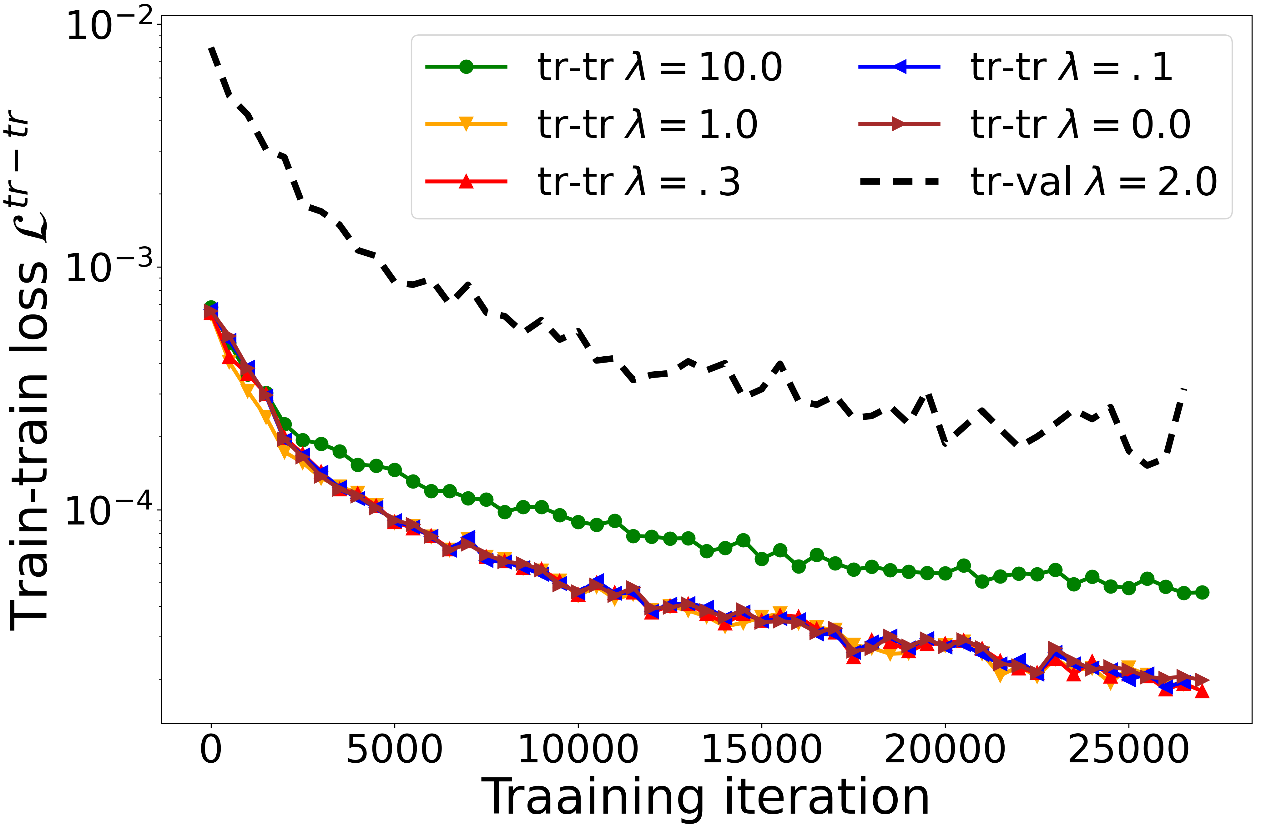
(d)

Figure 4: Plot of singular values and t-SNE plots for iMAML tr-val versus tr-tr. (a): Singular values for representations produced by tr-val versus tr-tr of a CNN model trained with iMAML on Omniglot 5-way 1-shot. (b): t-SNE plot of representations produced by tr-val CNN model trained with iMAML on Omniglot 5-way 1-shot for 10 randomly selected classes of test split. (c): t-SNE plot of representations produced by tr-tr CNN trained with iMAML model on Omniglot 5-way 1-shot for the same 10 randomly selected classes of test split. We find that the tr-val representations appear to be more clustered than the tr-tr representations. (d): Tr-tr loss values for tr-tr versus tr-val models.

We train a model on Omniglot 5-way 1-shot using iMAML with batch size 32, inner learning rate .05, and meta steps 30000, again using the original author code convolutional neural network. We use $\lambda=2.0$ for tr-val and $\lambda=1.0$ for tr-tr. We use the tr-val and tr-tr CNN models to get image representations for input images, and then perform t-SNE on 10 randomly selected classes. We report t-SNE and singular value decay results for iMAML in Figure 4. We also plot the t-SNE representations for varying values of the perplexity in Figure 2. As in the case of RepLearn, the tr-val representations are much better clustered in the tr-tr representations. Furthermore the tr-val representations have a sharper drop in singular values, suggesting that they have lower effective rank than tr-tr representations.

Rank and Expressivity

For a fully connected model of width factor $\ell=32$ trained with RepLearn on Omniglot 5-way 1-shot, we conduct linear regression twice. The first regression predicts the tr-tr representations given the tr-val representations, and the second predicts the tr-val representations given the tr-tr representations. We find that the $R^{2}$ scores were $0.0973$ and $0.0967$, respectively. Thus the two sets of representations can express each other well enough, even though tr-val representations have lower effective rank.

We conduct the same experiment for a CNN model trained with iMAML on Omniglot 5-way 1-shot, and find that the $R^{2}$ scores were 0.0103 and 0.171, respectively, thus suggesting that tr-val representations are a bit more expressive than tr-tr representations, in addition to having lower effective rank.

Figure 2: t-SNE plots for tr-val versus tr-tr for varying values of the perplexity for a CNN model trained with iMAML on Omniglot 5-way 1-shot. Plots shown for 10 randomly selected classes from the test split of Omniglot. Top row depicts tr-tr and bottom row depicts tr-val. We find that the tr-val representations appear to be more clustered for all values of perplexity of t-SNE.

Adding explicit regularization to RepLearn

For a CNN model trained with RepLearn on Omniglot 5-way 1-shot, we add explicit regularization to tr-tr by adding the Frobenius norm of the representation to the loss. We report the accuracy in percentage evaluated on 1200 tasks in Table 8 in the top row. We find that this significantly improves the performance of the tr-tr method, compared to the tr-tr models without explicit regularization in Table 10, or the bottom row of Table 8. This fits our intuition that the tr-tr method requires some form of regularization to learn low rank representations and to have guaranteed good performance on new tasks.

D.3 MiniImageNet Experiments

RepLearn on MiniImageNet

As standard [Rajeswaran et al., 2019], we resize the data to 84x84 pixel images and apply 90, 180, and 270 degree rotations and use a batch size of 16 during training. We use a convolutional neural network with four convolutional layers, with output filter sizes of 32,, 64, 128, and 128 each followed by batch normalization and ReLU activations. We investigate the performance of tr-val versus tr-tr for RepLearn on the MiniImageNet 5-way 1-shot and 5-way 5-shot setting and report our results in Table 7. The findings are very similar to those from the Omniglot dataset, suggesting that our insights hold across multiple benchmark datasets.

Table 7: Tr-val versus tr-tr meta-test accuracies in % for a CNN model trained with RepLearn on MiniImageNet 5-way 1-shot and 5-way 5-shot for varying values of the regularization parameter, $\lambda$. The final value of the tr-tr objective is depicted in the last two columns for MiniImageNet 5-way 1-shot and MiniImageNet 5-way 5-shot, respectively. The tr-tr models make the tr-tr loss very small, which is what they were trained to minimize. Thus their failure on few-shot learning is not due to failure of optimization.

	5-way 1-shot	5-way 5-shot	tr-tr loss 5-way 1-shot	tr-tr loss 5-way 5-shot
$\lambda=$ 0.0 tr-val	46.16 $\pm$ 1.67	65.36 $\pm$ 0.91	0.01	0.01
$\lambda=$ 0.0 tr-tr	25.53 $\pm$ 1.43	33.49 $\pm$ 0.82	1.1e-8	2.1e-6
$\lambda=$ 0.1 tr-tr	24.69 $\pm$ 1.32	34.91 $\pm$ 0.85	3.5e-8	5.5e-7
$\lambda=$ 1.0 tr-tr	25.88 $\pm$ 1.45	40.19 $\pm$ 1.12	1.9e-6	9.3e-5

Increasing capacity of a CNN model on MiniImageNet

We start with a CNN model trained on MiniImageNet with four convolutional layers with 32, 64, 128, and 128 filters, respectively. Each convolution is followed by batch normalization and ReLU activations. We train with RepLearn. We increase the capacity by increasing the number of filters by a capacity factor, $\ell$, so that the convolutional layers contain $32\ell$, $64\ell$, $128\ell$, and $128\ell$ output filters, respectively. We depict our results in Table 9. We find that increasing the network capacity improves the performance of tr-val representations, but slightly hurts tr-tr performance, just like the findings for Omniglot dataset with fully-connected networks. Thus the tr-val method is more robust to architecture choice/capacity and datasets.

t-SNE on MiniImageNet

We take the baseline convolutional neural network with capacity factor $\ell=1$ from the previous section, and conduction t-SNE on the representations produced by the tr-val versus the tr-tr model. We report our results in Figure 3.

Table 8: Meta-test accuracies in % for tr-tr RepLearn trained on Omniglot 5-way 1-shot with explicit Frobenius norm regularization added to the representations.

	$\lambda=$ 0.0 (tr-tr)	$\lambda=$ 0.1 (tr-tr)	$\lambda=$ 3.0(tr-tr)
with representation regularization	94.73 $\pm$ 0.55	95.05 $\pm$ 0.55	94.74 $\pm$ 0.55
no representation regularization	67.78 $\pm$ 1.60	67.53 $\pm$ 1.66	89.00 $\pm$ 1.08

Table 9: Accuracies in % of representations parameterized by CNN networks of varying number of filters on MiniImageNet. Representations trained using tr-val objective consistently outperforms those learned using tr-tr objective, and the gap increases as width increases.

capacity $=$	MiniImageNet 5-way 1-shot		Supervised 20-way
$num\_filters^{*}\ell$	tr-val	tr-tr	tr-val	tr-tr
$\ell=0.5$	46.66 $\pm$ 1.69	26.25 $\pm$ 1.45	1.	1.
$\ell=1$	48.44 $\pm$ 1.62	26.81 $\pm$ 1.44	1.	1.
$\ell=4$	52.22 $\pm$ 1.68.	24.66 $\pm$ 1.26	1.	1.
$\ell=8$	52.25 $\pm$ 1.71	25.28 $\pm$ 1.37	1.	1.

Table 10: Tr-val versus tr-tr meta-test accuracies in % for a CNN model trained with RepLearn on Omniglot 5-way 1-shot for varying values of the regularization parameter, $\lambda$.

	5-way 1-shot tr-val	5-way 1-shot tr-tr
$\lambda=$ 0.0	97.25 $\pm$ 0.57	67.78 $\pm$ 1.60
$\lambda=$ 0.1	97.34 $\pm$ 0.59	67.53 $\pm$ 1.64
$\lambda=$ 0.3	97.59 $\pm$ 0.55	66.06 $\pm$ 1.67
$\lambda=$ 1.0	97.66 $\pm$ 0.52	87.25 $\pm$ 1.13
$\lambda=$ 3.0	97.19 $\pm$ 0.59	89.00 $\pm$ 1.08
$\lambda=$ 10.0	96.50 $\pm$ 0.61	85.41 $\pm$ 1.22

Table 11: Tr-val versus tr-tr meta-test accuracies in % for a CNN model trained with RepLearn on Omniglot 20-way 1-shot for varying values of the regularization parameter, $\lambda$.

	20-way 1-shot trval	20-way 1-shot tr-tr
$\lambda=$ 0.0	92.26 $\pm$ 0.45	49.00 $\pm$ 0.88
$\lambda=$ 0.1	92.38 $\pm$ 0.44	50.84 $\pm$ 0.85
$\lambda=$ 0.3	92.21 $\pm$ 0.47	55.38 $\pm$ 0.92
$\lambda=$ 1.0	92.44 $\pm$ 0.47	84.14 $\pm$ 0.63
$\lambda=$ 3.0	92.70 $\pm$ 0.48	88.20 $\pm$ 0.55
$\lambda=$ 10.0	91.50 $\pm$ 0.48	85.85 $\pm$ 0.58

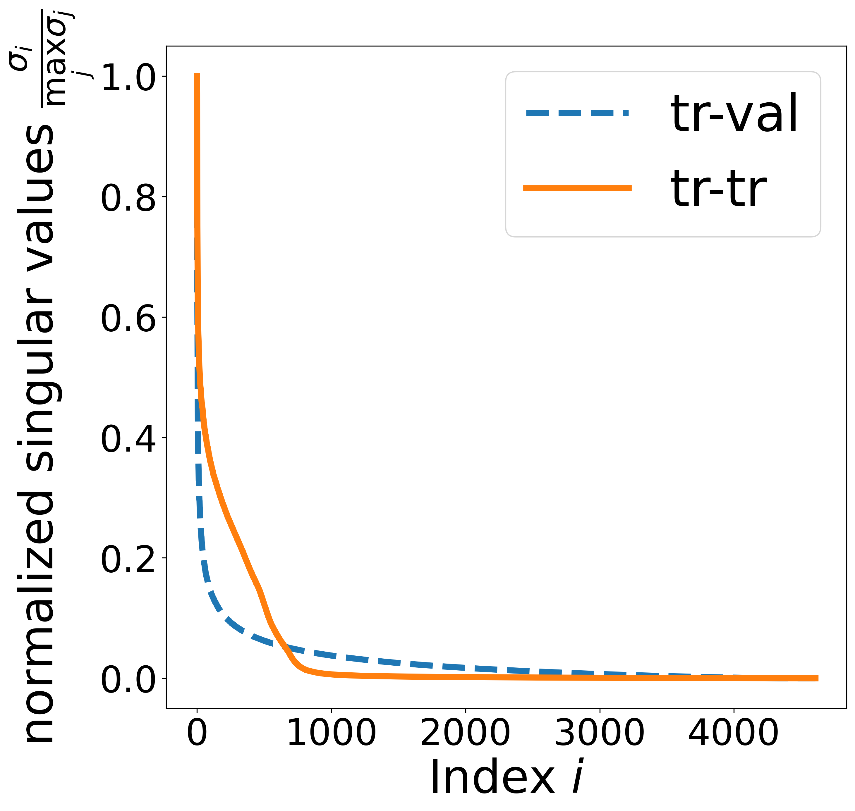
(a)

(b)

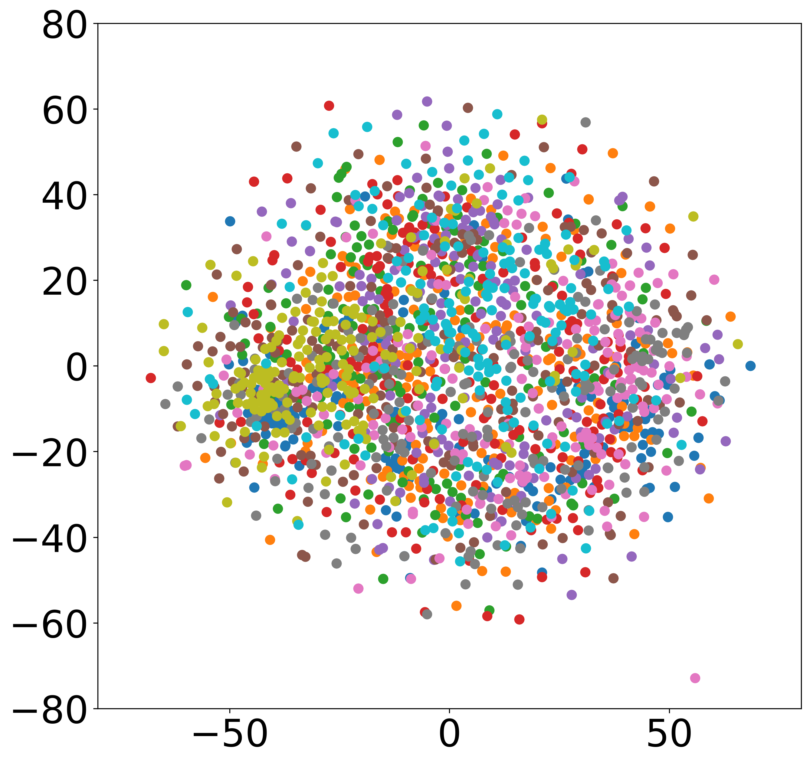
(c)

Figure 3: Plot of singular values and t-SNE plots for MiniImageNet tr-val versus tr-tr. (a): Singular values for representations produced by tr-val versus tr-tr of a CNN model trained with RepLearn on MiniImagement. (b): t-SNE plot of representations produced by tr-val CNN model trained with RepLearn on MiniImageNet for 10 randomly selected classes of test split. (c): t-SNE plot of representations produced by tr-tr CNN model trained with RepLearn on MiniImageNet for the same 10 randomly selected classes of test split. We find that the tr-val representations appear to be more clustered than the tr-tr representations.

(a)

(b)

(c)

References

- Ahn and Brewer (1993) Woo-Kyoung Ahn and William F Brewer. Psychological studies of explanation—based learning. Investigating explanation-based learning, 1993.
- Alquier et al. (2017) Pierre Alquier, The Tien Mai, and Massimiliano Pontil. Regret bounds for lifelong learning. In Proceedings of the 20th International Conference on Artificial Intelligence and Statistics, 2017.
- Andrychowicz et al. (2016) Marcin Andrychowicz, Misha Denil, Sergio Gómez, Matthew W Hoffman, David Pfau, Tom Schaul, Brendan Shillingford, and Nando de Freitas. Learning to learn by gradient descent by gradient descent. In Advances in Neural Information Processing Systems, 2016.
- Argyriou et al. (2008) Andreas Argyriou, Theodoros Evgeniou, and Massimiliano Pontil. Convex multi-task feature learning. Machine learning, 2008.
- Arnold et al. (2019) Sébastien MR Arnold, Shariq Iqbal, and Fei Sha. When maml can adapt fast and how to assist when it cannot. arXiv preprint arXiv:1910.13603, 2019.
- Bai et al. (2020) Yu Bai, Minshuo Chen, Pan Zhou, Tuo Zhao, Jason D Lee, Sham Kakade, Huan Wang, and Caiming Xiong. How important is the train-validation split in meta-learning? arXiv preprint arXiv:2010.05843, 2020.
- Baxter (2000) Jonathan Baxter. A model of inductive bias learning. Journal of Artificial Intelligence Research, 2000.
- Belkin et al. (2020) Mikhail Belkin, Daniel Hsu, and Ji Xu. Two models of double descent for weak features. SIAM Journal on Mathematics of Data Science, 2020.
- Bengio et al. (1990) Yoshua Bengio, Samy Bengio, and Jocelyn Cloutier. Learning a synaptic learning rule. Citeseer, 1990.
- Bertinetto et al. (2019) Luca Bertinetto, Joao F. Henriques, Philip Torr, and Andrea Vedaldi. Meta-learning with differentiable closed-form solvers. In International Conference on Learning Representations, 2019.
- Bullins et al. (2019) Brian Bullins, Elad Hazan, Adam Kalai, and Roi Livni. Generalize across tasks: Efficient algorithms for linear representation learning. In Proceedings of the 30th International Conference on Algorithmic Learning Theory, 2019.
- Caruana (1997) Rich Caruana. Multitask learning. Machine learning, 28, 1997.
- Collins et al. (2020) Liam Collins, Aryan Mokhtari, and Sanjay Shakkottai. Why does maml outperform erm? an optimization perspective. arXiv preprint arXiv:2010.14672, 2020.
- Deleu et al. (2019) Tristan Deleu, Tobias Würfl, Mandana Samiei, Joseph Paul Cohen, and Yoshua Bengio. Torchmeta: A Meta-Learning library for PyTorch, 2019. Available at: https://github.com/tristandeleu/pytorch-meta.
- Denevi et al. (2018a) Giulia Denevi, Carlo Ciliberto, Dimitris Stamos, and Massimiliano Pontil. Incremental learning-to-learn with statistical guarantees. In Proceedings of the Conference on Uncertainty in Artificial Intelligence, 2018a.
- Denevi et al. (2018b) Giulia Denevi, Carlo Ciliberto, Dimitris Stamos, and Massimiliano Pontil. Learning to learning around a common mean. In Advances in Neural Information Processing Systems, 2018b.
- Du et al. (2020) Simon S Du, Wei Hu, Sham M Kakade, Jason D Lee, and Qi Lei. Few-shot learning via learning the representation, provably. arXiv preprint arXiv:2002.09434, 2020.
- Evgeniou and Pontil (2004) Theodoros Evgeniou and Massimiliano Pontil. Regularized multi-task learning. In Proceedings of the 10th ACM SIGKDD International Conference on Knowledge Discovery and Data Mining, 2004.
- Fallah et al. (2020) Alireza Fallah, Aryan Mokhtari, and Asuman Ozdaglar. On the convergence theory of gradient-based model-agnostic meta-learning algorithms. 2020.
- Finn et al. (2017) Chelsea Finn, Pieter Abbeel, and Sergey Levine. Model-agnostic meta-learning for fast adaptation of deep networks. In Proceedings of the 34th International Conference on Machine Learning, 2017.
- Goldblum et al. (2020) Micah Goldblum, Steven Reich, Liam Fowl, Renkun Ni, Valeriia Cherepanova, and Tom Goldstein. Unraveling meta-learning: Understanding feature representations for few-shot tasks. In Proceedings of the 37th International Conference on Machine Learning, 2020.
- Gu et al. (2018) Jiatao Gu, Yong Wang, Yun Chen, Victor O. K. Li, and Kyunghyun Cho. Meta-learning for low-resource neural machine translation. In Proceedings of the 2018 Conference on Empirical Methods in Natural Language Processing, 2018.
- Khodak et al. (2019a) Mikhail Khodak, Maria-Florina Balcan, and Ameet Talwalkar. Adaptive gradient-based meta-learning methods. In Advances in Neural Information Processing Systems, 2019a.
- Khodak et al. (2019b) Mikhail Khodak, Maria-Florina Balcan, and Ameet Talwalkar. Provable guarantees for gradient-based meta-learning. In Proceedings of the 36th International Conference on Machine Learning, 2019b.
- Kong et al. (2020) Weihao Kong, Raghav Somani, Zhao Song, Sham Kakade, and Sewoong Oh. Meta-learning for mixed linear regression. In International Conference on Machine Learning, 2020.
- Lake et al. (2015) Brenden M Lake, Ruslan Salakhutdinov, and Joshua B Tenenbaum. Human-level concept learning through probabilistic program induction. Science, 2015.
- Lee et al. (2019) Kwonjoon Lee, Subhransu Maji, Avinash Ravichandran, and Stefano Soatto. Meta-learning with differentiable convex optimization. In Proceedings of the IEEE/CVF Conference on Computer Vision and Pattern Recognition, 2019.
- Mardia et al. (1979) KV Mardia, JT Kent, and JM Bibby. Multivariate analysis, 1979. Probability and mathematical statistics. Academic Press Inc, 1979.
- Maurer (2005) Andreas Maurer. Algorithmic stability and meta-learning. Journal of Machine Learning Research, 6, 2005.
- Maurer (2009) Andreas Maurer. Transfer bounds for linear feature learning. Machine Learning, 2009.
- Maurer and Pontil (2013) Andreas Maurer and Massimiliano Pontil. Excess risk bounds for multitask learning with trace norm regularization. In Proceedings of the 26th Annual Conference on Learning Theory, 2013.
- Maurer et al. (2016) Andreas Maurer, Massimiliano Pontil, and Bernardino Romera-Paredes. The benefit of multitask representation learning. Journal of Machine Learning Research, 17, 2016.
- McMahan et al. (2017) H. Brendan McMahan, Eider Moore, Daniel Ramage, Seth Hampson, and Blaise Aguera y Arcas. Communication-efficient learning of deep networks from decentralized data. In Proceedings of the 20th International Conference on Artifical Intelligence and Statistics, 2017.
- Naik and Mammone (1992) Devang K Naik and Richard J Mammone. Meta-neural networks that learn by learning. In [Proceedings 1992] IJCNN International Joint Conference on Neural Networks. IEEE, 1992.
- Nichol et al. (2018) Alex Nichol, Joshua Achiam, and John Schulman. On first-order meta-learning algorithms. arXiv preprint arXiv:1803.02999, 2018.
- Oh et al. (2020) Jaehoon Oh, Hyungjun Yoo, ChangHwan Kim, and Se-Young Yun. Does maml really want feature reuse only? arXiv preprint arXiv:2008.08882, 2020.
- Pentina and Lampert (2014) Anastasia Pentina and Christoph H. Lampert. A PAC-Bayesian bound for lifelong learning. In Proceedings of the 31st International Conference on Machine Learning, 2014.
- Raghu et al. (2020) Aniruddh Raghu, Maithra Raghu, Samy Bengio, and Oriol Vinyals. Rapid learning or feature reuse? Towards understanding the effectiveness of MAML. In Proceedings of the 8th International Conference on Learning Representations, 2020.
- Rajeswaran et al. (2019) Aravind Rajeswaran, Chelsea Finn, Sham M. Kakade, and Sergey Levine. Meta-learning with implicit gradients. In Advances in Neural Information Processing Systems, 2019.
- Ravi and Larochelle (2017) Sachin Ravi and Hugo Larochelle. Optimization as a model for few-shot learning. In Proceedings of the 5th International Conference on Learning Representations, 2017.
- Ruvolo and Eaton (2013) Paul Ruvolo and Eric Eaton. ELLA: An efficient lifelong learning algorithm. In Proceedings of the 30th International Conference on Machine Learning, 2013.
- Saunshi et al. (2020) Nikunj Saunshi, Yi Zhang, Mikhail Khodak, and Sanjeev Arora. A sample complexity separation between non-convex and convex meta-learning. In International Conference on Machine Learning, 2020.
- Schmidhuber (1987) Jürgen Schmidhuber. Evolutionary principles in self-referential learning, or on learning how to learn. PhD thesis, Technische Universität München, 1987.
- Snell et al. (2017) Jake Snell, Kevin Swersky, and Richard S. Zemel. Prototypical networks for few-shot learning. In Advances in Neural Information Processing Systems, 2017.
- Thrun and Pratt (1998) Sebastian Thrun and Lorien Pratt. Learning to Learn. Springer Science & Business Media, 1998.
- Tripuraneni et al. (2020a) Nilesh Tripuraneni, Chi Jin, and Michael I Jordan. Provable meta-learning of linear representations. arXiv preprint arXiv:2002.11684, 2020a.
- Tripuraneni et al. (2020b) Nilesh Tripuraneni, Michael I Jordan, and Chi Jin. On the theory of transfer learning: The importance of task diversity. 2020b.
- Vinyals et al. (2016) Oriol Vinyals, Charles Blundell, Timothy Lillicrap, Koray Kavukcuoglu, and Daan Wierstra. Matching networks for one shot learning. In Advances in Neural Information Processing Systems, 2016.
- Wang et al. (2020a) Haoxiang Wang, Ruoyu Sun, and Bo Li. Global convergence and induced kernels of gradient-based meta-learning with neural nets. arXiv preprint arXiv:2006.14606, 2020a.
- Wang et al. (2020b) Xiang Wang, Shuai Yuan, Chenwei Wu, and Rong Ge. Guarantees for tuning the step size using a learning-to-learn approach. arXiv preprint arXiv:2006.16495, 2020b.
- Zhou et al. (2019) Pan Zhou, Xiaotong Yuan, Huan Xu, Shuicheng Yan, and Jiashi Feng. Efficient meta learning via minibatch proximal update. In Advances in Neural Information Processing Systems, 2019.