Metallic Hydrogen: A Liquid Superconductor?

Abstract

Metallic hydrogen is expected to exhibit remarkable physics. Of particular interest in this work is the possibility of high-temperature superconductivity. Comparing calculations of the superconducting critical temperatures of the solid phase to melting temperatures over a range of pressures leads to an interesting question: Will the solid, in a superconducting state, melt to a liquid that remains a superconductor? In this work, the possibility of liquid superconductivity in metallic hydrogen is investigated. This is done by first-principles simulations, and using the results of these to solve the Eliashberg equations. These are carried out over the pressure (and temperature) conditions where molecular dissociation is expected to first occur in the solid phase. Over the pressure range $386.8(4)$–$783.7(4)$ GPa, $T_{c}$ increases from $308(6)$ to $372(2)$ K with a maximum uncertainty of $10$ K; it then decreases to $356(2)$ K at $883.7(3)$ GPa. Comparisons to the solid phase show that the critical temperature is not significantly changed between the two phases, though the physics behind their superconductivity is different. Careful comparisons of these values to recent results in the context of the hydrogen phase diagram show that they are higher than the melting temperatures and that the solid will melt to liquid atomic hydrogen. The results of this work (in this context) therefore suggest that liquid atomic hydrogen will indeed exist in a superconducting state. They also provide the pressure and temperature conditions over which to look for it.

I Introduction

Hydrogen is the most abundant element in the Universe, comprising roughly $74$% of all baryonic matter. Despite its chemical simplicity (a single proton and electron), its behavior over a wide range of thermodynamic conditions is remarkably complex. This can be seen, for example, in the hydrogen phase diagram, as shown in Fig. 1.

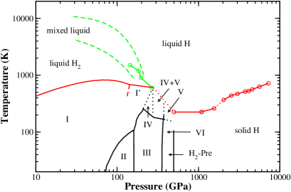
Figure 1: Phase diagram of hydrogen. Data combined from experimental and computational studies Liu et al. (2017); Eremets and Troyan (2011); Eremets et al. (2016); Dalladay-Simpson et al. (2016); Dias et al. (2019); McMinis et al. (2015); Dias and Silvera (2017); eaa (2017); Zha et al. (2017); Liu et al. (2013); Geng et al. (2015); Geng and Wu (2016); Jiang et al. (2020); Pierleoni et al. (2016).

(Many of the specific details of this diagram are not necessary to consider; rather, this diagram will be used for reference during discussion herein.) With this complexity comes remarkably rich physics. Of interest in this work are the properties of dense hydrogen (in particular, as caused by high pressures). These have been generally reviewed in Ref. McMahon et al., 2012, and those of particular interest are done so below.

In 1935, Wigner and Huntington predicted Wigner and Huntington (1935) that sufficient pressure would dissociate hydrogen molecules, and that any Bravais lattice of such atoms would be metallic. The pressures required to dissociate hydrogen molecules are expected to be significant [$447(3)$ GPa according to computation McMinis et al. (2015), consistent with experiment that shows Eremets et al. (2019) at least above $440$ GPa, possibly near $495$ GPa Dias and Silvera (2017); eaa (2017)]. This transition can be seen by the vertical line in Fig. 1.

In 1968, Ashcroft predicted Ashcroft (1968) another type of transition, a metallic-to-superconducting one. Within the framework of Bardeen–Cooper–Schrieffer (BCS) theory Bardeen et al. (1957a, b), three arguments were made to support this prediction: (i) the ions in the system are single protons, and their small mass causes the vibrational energy scale of the phonons to be remarkably high (this generally enters as a prefactor in approximate expressions for the superconducting critical temperature $T_{c}$); (ii) since the electron–ion interaction is due to the bare Coulomb attraction, the electron–phonon coupling should be strong; and (iii) at the high pressures at and above metallization, the electronic density of states $N(0)$ at the Fermi surface should be large and the Coulomb repulsion between electrons relatively low. Recent calculations Borinaga et al. (2016) near the (solid) molecular-to-atomic transition give a value of $T_{c}=300$ K at $500$ GPa. Calculations McMahon and Ceperley (2011a, 2012) further show an increase with increasing pressure with a maximum near $700$ GPa.

Recent calculations of the melting line of the atomic solid Liu et al. (2013); Geng et al. (2015) (discussed above) show that it melts around $200$–$250$ K near and just above the pressure of molecular dissociation. This range is indicated on the phase diagram in Fig. 1 as a horizontal line at $225$ K. (A more thorough and specific discussion of these results is reserved for later, so that they can be considered in the context of those presented herein.) If these results are considered with those above, it can be seen that the $T_{c}$ values are even higher. This leads to an interesting question: Will the solid, in a superconducting state, melt to a liquid that remains a superconductor?

In 1981, Jaffe and Ashcroft gave Jaffe and Ashcroft (1981) two reasons for why liquid superconductors could theoretically exist: (i) compressibility of metals changes very little during melting, and so high-frequency, longitudinal phonons should be similar in both the solid and liquid phases; and (ii) the existence of amorphous superconductors indicates that disorder does not inhibit superconductivity. For all classical metals, however, BCS liquid superconductors seem almost implausible. Arguments Edwards et al. (2006) based on comparisons of $T_{c}$ to melting temperatures have been used to show this. This is not the case though for quantum metals — systems with large quantum zero-point motion of the ions that may strongly depress the (classical) melting melting temperature. This would be the case, for example, for some light elements. The resultant liquid must also be metallic though, meaning that dense hydrogen might be the only such system where this would be plausible. This problem has received relatively little attention, however. And now that experiments (such as those discussed above, and will also be discussed below) are now capable of or are approaching the relevant thermodynamic conditions makes it a timely problem to consider.

In this Article, the possibility of superconductivity in liquid atomic hydrogen is investigated by first-principles simulations, and using the results of these to solve the Eliashberg equations Éliashberg (1960). This is done over thermodynamic conditions where molecular dissociation is expected to first occur and where superconductivity in the liquid would be most likely (if it occurs at all). This would be approximately $350$–$850$ GPa and less than $500$ K.

This Article is outlined as follows. In the next section (Section II), a method is carefully considered to calculate properties associated with superconductivity for a liquid phase. Section III presents and discusses the results from the application of this method to liquid atomic hydrogen. Section IV concludes, by discussing these results in the context of the hydrogen phase diagram and current experimental techniques.

II Methods

Calculating superconductivity properties is relatively straightforward for a solid, by using methods developed to study lattice dynamics. Things become more involved when considering a liquid, due to dynamical motion. Under some careful considerations and reasonable approximations though, it is possible to leverage and apply the aforementioned methods to the system of interest.

The method considered in this work consists of the following steps:

1. Optimization of starting solid structures, to determine constant volumes representative of desired pressures.

2. Molecular dynamics simulations, to melt the solids and then simulate the liquid at constant temperature.

3. Determination of statistically-independent configurations representative of the liquid.

4. Calculation of phonons and more specific superconductivity properties (of the liquid).

These steps are described in detail in this section.

II.1 Electronic-structure calculations

All calculations were performed using the Quantum ESPRESSO (QE) density-functional theory Jones (2015) (DFT) code Giannozzi et al. (2009). See Ref. Tenney et al., 2020 (and its Supplementary Information) for a discussion on the justification of the use of DFT, and some of the following settings, to study atomic hydrogen. The pseudopotential approximation based on the projector augmented wave method Kresse and Joubert (1999) was used pse to replace the bare Coulomb potential of the protons. The Perdew–Burke–Ernzerhof generalized gradient approximation exchange–correlation functional Perdew et al. (1996) was used. QE is based on a plane-wave basis set. Kinetic-energy cutoffs for the wavefunction and charge density and potential are specified in the context of specific calculations below. The same is done for Brillouin-zone sampling ($\mathbf{k}$ points). The smearing scheme of Methfessel–Paxton Methfessel and Paxton (1989) was used for integrations based on this sampling. Note that this is “cold” (zero-temperature) smearing technique, but this does not affect the results in this work since finite-temperature free energies are not needed.

II.2 Geometry optimizations

Pressures were chosen over which hydrogen is expected to first be atomic, metallic, and a liquid. (Ground-state) pressures were chosen every $100$ GPa from $350$ to $850$ GPa.

The starting (ground-state) structures are unit cells of the body-centered cubic lattice. This lattice was chosen, as it has been found McMahon and Ceperley (2011b) to be one of the most dynamically unstable structures over the pressure range considered. Therefore, it should therefore immediately melt to liquid. Indeed, earlier simulations of the melting line of atomic hydrogen Xu et al. (1994); Kohanoff and Hansen (1995, 1996) find that this lattice may melt at surprisingly low temperatures over the considered pressure range.

The stationary point of each structure (both lattice vectors and ion positions) at each pressure was found by performing constant-pressure geometry optimizations. Recommended kinetic-energy cutoffs of $46$ Ry for the wavefunction and $221$ Ry for the charge density and potential were used for the chosen pseudopotential. For Brillouin-zone sampling, at least $5{\times}5{\times}5$ (shifted) $\mathbf{k}$ points (for a $16$-particle system, for example; this number is scaled precisely for larger ones) were used. Optimizations were done using the Broyden–Fletcher–Goldfarb–Shanno algorithm Fletcher (1987), as implemented within QE. Pressures were converged to within $0.1$ GPa.

II.3 Molecular dynamics

Atomic configurations representative of liquid atomic hydrogen were generated consistent with the canonical ensemble (constant $NVT$ where $N$, $V$, and $T$ are number of particles, volume, and temperature, respectively). Several simulations were carried out using a number of particles from $16$ to $250$. Comparisons between simulations were made as a test of convergence with respect to system size. Initial volumes were determined from the geometry optimizations (discussed above). Choosing the temperature involves several considerations: Relevant liquid configurations are those at or below the superconducting critical temperature, but this is a priori unknown. Therefore, in order to determine whether this even occurs at all, temperatures should be chosen just above melting. Classical melting temperatures are calculated Liu et al. (2013); Geng et al. (2015) around $350$ K and flat or slight positive slope with pressure over the range considered herein. In addition, the classical superheating degree is calculated Geng et al. (2015) to be about $100$ K. With all of these considerations, a temperature of $500$ K was chosen. Note that these calculations also show an importance of nuclear quantum effects of just over $100$ K. This suggests that the $500$ K (classical) liquid may be representative of the actual (quantum effects included) at lower temperatures. Temperature was controlled using the Andersen thermostat Andersen (1980), a thermostat which is consistent with the canonical ensemble. This thermostat is specified by a single parameter — the collision frequency $\nu$, which was set to a relatively low value (to be discussed below) of $0.002$ Ry.

Configurations were generated from Born–Oppenheimer molecular dynamics simulations. These were based on DFT. Kinetic-energy cutoffs and Brillouin-zone sampling were the same as for geometry optimizations (discussed above). The time step was set to as $10$ Ry ($1$ a.u. $=$ $4.8378\times 10^{-17}$ s). Simulations were carried out in two steps: a first one of $2048$ steps to equilibrate (melt to a liquid), followed by a second one of $16384$ steps to generate enough liquid configurations for statistical analysis (discussed below).

II.4 Liquid configurations

From the generated configurations (discussed above), random ones were selected as representative of the liquid. Properties of the liquid were then calculated as averages over these, with the mean and sample standard deviation of the mean reported. While this is correct for many properties of interest, careful consideration must be made for dynamical ones (as static configurations are only approximate, if at all). These are discussed in context below.

Note that at finite temperature, a configuration of a (classical) liquid can be considered as a random thermal fluctuation about any inherent structure. Because it is this local potential-energy minimum that is of interest in the calculation of properties, less-aggressive relaxations (in this case, at constant volume) of these configurations were performed. These were carried out using the damped Verlet algorithm Verlet (1967), as implemented within QE. Forward looking to the following calculations, settings for the DFT calculations were increased for convergence. Cutoffs were increased to $57.5$ and $345.5$ Ry for the wavefunction and charge density and potential, respectively. The number of $\mathbf{k}$ points for Brillouin-zone sampling was increased to $16{\times}16{\times}16$ (unshifted), which is sufficiently dense to include both the full (fine) grid and an $8{\times}8{\times}8$ (course) one, which are both needed (as discussed below).

II.5 Phonons

Phonons are one of the main properties of interest. Of particular interest is the phonon density of states $F(\omega)$ as a function of frequency $\omega$. These were calculated by two approaches.

Phonons of the dynamical liquid were calculated directly from the molecular dynamics simulations, by a Fourier transform of the velocity autocorrelation function. Note that the Andersen thermostat is stochastic, and so comparisons were made against the Berendsen thermostat Berendsen et al. (1984) (a thermostat which is deterministic, but not rigorously consistent with the canonical ensemble), to ensure that the value of $\nu$ is low enough such that it does not significantly affect correlations.

Due to the small proton mass, the magnitude of the phonon frequencies is expected to be considerable in hydrogen. On the timescale of translation (by diffusion through the liquid), the atoms will have oscillated a number of times. This suggests that static configurations can be used as representative of the liquid. This was verified by comparing the following calculations to the corresponding dynamical ones (discussed above). Phonons for static configurations were calculated using density-functional perturbation theory Baroni et al. (2001), as implemented within QE. These were calculated with a $\mathbf{k}$-point grid of $8{\times}8{\times}8$. A $4{\times}4{\times}4$ grid of $\mathbf{q}$ points was used, to calculate the phonon density of states $F(\omega)$. This value was found to be sufficient for convergence, consistent with Ref. McMahon and Ceperley, 2011a, 2012. Note that these calculations are based on the harmonic approximation. Anharmonic effects in atomic hydrogen have been studied in Ref. Borinaga et al., 2016. As far as the specific properties of interest herein, such effects are found to have only a relatively small impact. The results should therefore be considered (in this context) at least semi-quantitative.

II.6 Superconductivity

To calculate properties associated with superconductivity, the Eliashberg equations Éliashberg (1960) were used. This theory accurately describes strong electron–phonon interactions. The important microscopic parameters that enter into this theory are the (Eliashberg) spectral function $\alpha^{2}F(\omega)$ and Coulomb pseudopotential $\mu^{*}$. Within BCS theory, the electron–phonon interaction is the source of attraction that binds two electrons into a paired state. $\alpha^{2}F(\omega)$ describes this coupling, $\alpha^{2}(\omega)$ (it is squared, since two electrons are coupled) and $F(\omega)$ (discussed above). $\mu^{*}$ describes the strength of the effective Coulomb repulsion between the coupled electrons. The equations were numerical solved Szczȩśniak (2006) for the gap function, to find the superconducting critical temperature $T_{c}$ (the temperature at which this function goes to zero).

$\alpha^{2}F(\omega)$ was calculated using density-functional perturbation theory, as implemented within QE (the only input necessary from QE for this). A coarse grid of $8{\times}8{\times}8$ (unshifted) and dense one of $16{\times}16{\times}16$ (unshifted) of $\mathbf{k}$ points were used for the DFT calculations. Note that these values are fully consistent with the converged geometry relaxations (dense grid), and also the phonon calculations (which are calculated in both cases on the course grid). The $\mathbf{q}$-point grid as used for the phonon calculations was also used for these, which should be McMahon and Ceperley (2011a, 2012) sufficiently dense to converge the electron–phonon coupling. (Two $\mathbf{k}$-point grids are needed, as mentioned above, as the dense one must include all $\mathbf{k}$$+$$\mathbf{q}$ points.) $\alpha^{2}F(\omega)$ was then calculated using a Gaussian broadening that led to convergence by inspection. Note that for calculations based on this function, a small contribution of (expected) imaginary frequencies were removed from the static calculations, since they are not present in the dynamical (phonon) ones. The value of $\mu^{*}$ as calculated Richardson and Ashcroft (1997) from first principles for high-density atomic hydrogen is $0.089$. With an error of about $3$% though, the standard value (for a high-density system) of $0.1$ remains reasonable, and this value is used herein. The only remaining quantity to calculate is therefore $\alpha^{2}F(\omega)$. Finally, the density of states at the Fermi level has been calculated Yan et al. (2011) for atomic hydrogen over the pressure range considered. The value does not change much with pressure, and a value of $0.45$ states/Ry/spin was chosen.

III Results

(Finite-temperature) pressures were calculated from the molecular dynamics simulations. Those for each of the simulations is shown in Table 1.

$386.8(4)$

$485.0(4)$

$584.1(4)$

$683.9(4)$

$783.7(4)$

$883.7(3)$

Table 1: Pressure values (in GPa) (at $500$ K) considered in this work.

The range over the calculations is $386.8(4)$–$883.7(3)$ GPa. Note that while these pressures (technically) correspond to $500$ K, they are considered the pressure values for the purpose of plots (e.g., as a function of pressure), discussion, etc. In addition, the uncertainties are generally smaller than the symbols used in these plots, and are thus omitted thereon.

III.1 Phonons

$F(\omega)$ of (random, as examples for discussion purpose) single configurations from simulations of liquid metallic hydrogen at $386.8(4)$ and $883.7(3)$ GPa (the end points of pressure considered) are shown in Fig. 2.

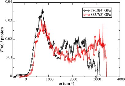
Figure 2: Phonon density of states $F(\omega)$ as a function of frequency $\omega$ at pressures of $386.8(4)$ and $883.7(3)$ GPa. Shown are those for a (random) single configuration for each pressure. Note that $F(\omega)$ has been normalized per proton, for quantitative comparisons here and below.

Note that, at a given pressure, while the atomic configurations appear qualitatively different (by inspection), the $F(\omega)$ are similar. This can be seen, for example, by comparing Fig. 2 with the following comparison between the liquid and solid phases [which plots a different $F(\omega)$ for the liquid for this comparison]. Any random configuration may therefore be considered representative of the liquid, for the purpose of discussion.

The magnitude of phonon frequencies become extremely large, reaching up to a few thousand cm^-1. Even $\langle\omega\rangle$ is large, around $1000$ cm^-1. This is considerable, considering for conventional metals $\langle\omega\rangle\approx 70$ cm^-1. This is expected though, considering the small mass of the proton that should result in high-frequency phonons. Calculations McMahon and Ceperley (2011b) for the solid atomic phase have shown this as the basis for large zero-point energies, for example.

$F(\omega)$ also displays significant structure. In particular, there is considerable phonon density at both low and high frequencies. This suggests that the liquid supports both strong acoustic and optical phonons, respectively.

As the pressure is increases, the high-frequency phonons shift higher, which results in an even larger separation of the low- and high-frequency modes. The greater compression probably leads to deeper and more narrow potential-energy wells locally, which leads to larger vibrational frequencies. This effect should be less significant at low frequencies, for which the vibrational physics is different (atoms moving in phase).

A comparison of the liquid phonons to those calculated for the solid phase McMahon and Ceperley (2011a, 2012) shows that they are qualitatively similar. Recalculation of also the solid data at the considered pressures and calculation settings to provide the same level of convergence is shown in Fig. 3.

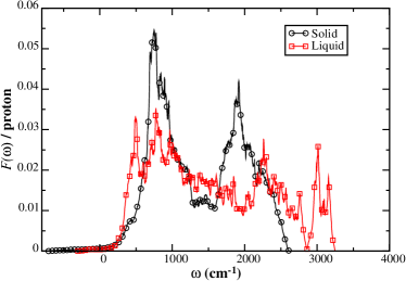
(a)

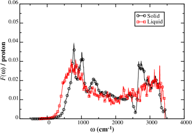
(b)

Figure 3: Comparison of $F(\omega)$ between the solid and liquid phases.

The agreement becomes noticeably better at higher pressures. At lower pressures, the high-frequency phonons in the solid occur at lower frequencies. At the higher pressures, the agreement also seems to be better at high frequencies. This is probably the result of that the low frequencies, acoustic phonons are those in which the ions move in phase, which in a liquid are expected to be much less likely. Overall, the agreement is consistent with the suggestions of Jaffe and Ashcroft Jaffe and Ashcroft (1981).

III.2 Electron–phonon coupling

In hydrogen, the electron–ion interaction is expected to be significant whether it is in the solid or liquid (or other) phase, as it arises from the bare Coulomb interaction. The electron–phonon interaction is therefore also expected to be high. $\alpha^{2}F(\omega)$ can be used to quantify this.

Figure 4 shows $\alpha^{2}F(\omega)$ for the two pressures, $386.8(4)$ and $883.7(3)$ GPa, considered above.

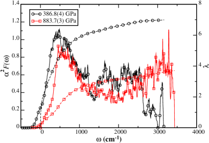
Figure 4: Eliashberg spectral function $\alpha^{2}F(\omega)$. The cumulative value of the expression in Eq. (1) in the text is plotted using dashed lines. The result of this integral over all $\omega$ is denoted by the electron–phonon coupling constant $\lambda$.

$\alpha^{2}F(\omega)$ follows the same trend as the phonon spectra in Fig. 2. This can be understood by considering that if $\alpha^{2}(\omega)$ is relatively flat (which means that the electron–ion interaction is relatively frequency-independent, and which appears to be the case here), then it is similar to $F(\omega)$.

While $\alpha^{2}F(\omega)$ contains all of the relevant information, consider the cumulative integral

$$2\int_{\omega_{\text{min}}}^{\omega_{\text{max}}}d\omega~{}\frac{\alpha^{2}F(\omega)}{\omega}$$ (1)

where ${\omega_{\text{min}}}$ and ${\omega_{\text{max}}}$ are minimum and maximum cutoff frequencies, respectively. This provides qualitative insight into the electron–phonon coupling over $[{\omega_{\text{min}}},{\omega_{\text{max}}}]$. This integral is plotted on the right axis in Fig. 4 from $0$ to $\omega$. At low frequencies, there is a rapid rise in it. It then only steadily does so at higher ones. It can therefore be concluded that lower frequencies are actually contributing the most to this coupling.

The total electron–phonon coupling constant is given by the range $[0,\infty)$, which is denoted by $\lambda$. That is, the total cumulative result of Eq. (1), which is also shown and indicated in Fig. 4 (for the two considered configurations). Figure 5 shows the average values of $\lambda$ over the pressure range considered.

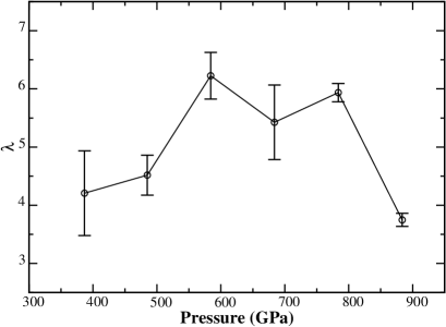
Figure 5: The value of $\lambda$ as a function of pressure.

The range of $\lambda$ is about $4$–$6$, which is very high. For common metals, $\lambda$ is below $0.5$. Morel and Anderson (1962) The high value of $\lambda$ puts it above the strong-coupling regime, given as $\lambda>1$. McMillan (1968) There is an increase of $\lambda$ with pressure, resulting in a maximum around $600$–$800$ GPa.

The magnitude of $\lambda$ is significantly higher (by a factor of about $2$–$3\times$) in the liquid than in the solid phase. For example, the calculation Borinaga et al. (2016) of $\lambda$ (including anharmonic effects) is $1.63$ at $500$ GPa. At least at the intermediate and higher pressures considered, this can be understood again considering $F(\omega)$, which has a greater density of phonons at low pressures (the low-frequency “peak” occurs at lower pressures, and the distribution is broader) (see again Fig. 3); this extends analogously to $\alpha^{2}F(\omega)$ (as discussed above), which causes Eq. (1) to integrate larger (because of the lower $\omega$). The trend with pressure is similar between the two phases though. Calculations McMahon and Ceperley (2011a, 2012) (not including anharmonic effects, but nonetheless agree well, at least at $500$ GPa) show an increase with pressure up to $700$ GPa before then decreasing.

III.3 Critical temperature

With the above information (and additional considerations discussed in Section II.6), the Eliashberg equations can be solved to find $T_{c}$. The value of $T_{c}$ as a function of pressure is shown in Fig. 6.

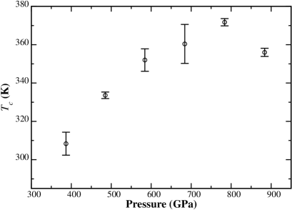
Figure 6: Superconducting critical temperatures $T_{c}$ as a function of pressure.

The values of $T_{c}$ are very high. The lowest value is $308(6)$ K at $386.8(4)$ GPa. It then increases semilinearly to $372(2)$ K at $783.7(4)$ GPa, before decreasing. This trend is consistent with those for the other quantities (discussed above), and can thus be understood in the context of those.

Again comparing to the solid phase, both the quantitative value (at $500$ GPa) Borinaga et al. (2016) and trends with pressure McMahon and Ceperley (2011a, 2012) are very similar. The physics though is slightly different. The phonon spectrum in the solid (understandably) has considerably more structure and which occur at higher frequencies (at least at relatively lower and intermediate pressures). This alone should result in larger values of $T_{c}$. However, it is for this precise reason that $\lambda$ has significantly lower values. Considered together, the $T_{c}$ values for the liquid and solid phases end up being similar.

IV Discussion & Conclusions

The superconducting critical temperatures of liquid atomic hydrogen have been calculated. Over the pressure range $386.8(4)$–$783.7(4)$ GPa, $T_{c}$ increases from $308(6)$ to $372(2)$ K with a maximum uncertainty of $10$ K; it then decreases to $356(2)$ K at $883.7(3)$ GPa. Comparisons to the solid phase show that the critical temperature is not significantly changed between the two phases, though the physics behind their superconductivity is different.

While the values of $T_{c}$ are remarkably high, whether this phase is realizable depends on the melting temperature of the solid. (The possibility of a metastable liquid is not considered in the following discussion, though this could be another approach to realization.) On the lower end of pressures considered, calculations predict the existence of a quasi-molecular mC24 phase Liu et al. (2012), in the pressure range between the stability fields of the molecular $Cmca$-$4$ phase Edwards et al. (1996) and atomic Cs-IV one McMahon and Ceperley (2011b). At higher pressures, the melting line of atomic hydrogen (including quantum effects) has been calculated Liu et al. (2013); Geng et al. (2015) to melt between around $200$–$250$ K and with a relatively flat change (or slight decrease) with pressure over the pressure range considered. (This decrease has also been calculated in Ref. Chen et al., 2013, though some of the quantitative aspects of these calculations have been shown Geng et al. (2015) to be incorrect.) And the melting temperature of the mC24 phase is systematically lower Liu et al. (2013). These lines are shown (near $225$ K) in Fig. 1. Calculations Liu et al. (2013) predict a second extremum (a minimum, in this case) in the melting line at the intersection of the melting lines of the molecular and atomic phases. Classically, this occurs at approximately $432$ GPa and $367$ K; but this is almost certainly reduced by nuclear quantum effects (that for the atomic phase alone would suggest about $100$ K), so for the purpose of discussion it will be considered near $300$ K. Note that the melting temperature (of the molecular phase) then increases with a reduction in pressure. This line (with the aforementioned suggested effects) is also shown in Fig. 1.

Another consideration is that the solid melts to a metallic state. A metallic liquid is necessary for superconductivity. There is a liquid–liquid phase transition (between molecular and atomic liquids), as also shown on Fig. 1. Calculations Gorelov et al. (2020) show closure of the fundamental electronic gap strongly correlates with the onset of molecular dissociation. This phase transition is perhaps most accurately and precisely known from calculations Pierleoni et al. (2016), and this line is also shown in Fig. 1. Along the $600$ K isotherm (the lowest temperature considered in the calculations), this transition is calculated to occur between approximately $267$ and $275$ GPa. Considering the decrease in temperature with pressure, an extrapolation to higher pressures would put it in the region of the aforementioned second extremum in the hydrogen melting line.

With all of the above considerations taken into account, it can be concluded that liquid atomic hydrogen will exist in a superconducting state. The lowest pressure at which this should be observable is near the second extremum at approximately $432$ GPa and around $300$ K. It is in this region where solid atomic hydrogen should melt to a liquid atomic phase. With an increase in $T_{c}$ with pressure (up to a maximum), and a flat or slight decrease in melting temperature, this state should also exist at higher pressures.

The main challenge is experimental, being able to reach the necessary thermodynamic conditions. Recent developments Zha et al. (2017) in heated diamond anvil cell techniques allow the study of hydrogen up to $300$ GPa at $295$–$1000$ K. This is approaching the necessary pressure and temperature conditions discussed herein. And the results of this work provide ones over which to look for this state.

References

- Liu et al. (2017) X.-D. Liu, R. T. Howie, H.-C. Zhang, X.-J. Chen, and E. Gregoryanz, Phys. Rev. Lett. 119, 065301 (2017).
- Eremets and Troyan (2011) M. I. Eremets and I. A. Troyan, Nature Materials 10, 927 (2011).
- Eremets et al. (2016) M. I. Eremets, I. A. Troyan, and A. P. Drozdov, “Low temperature phase diagram of hydrogen at pressures up to 380 gpa. a possible metallic phase at 360 gpa and 200 k,” (2016), arXiv:1601.04479 [cond-mat.mtrl-sci] .
- Dalladay-Simpson et al. (2016) P. Dalladay-Simpson, R. T. Howie, and E. Gregoryanz, Nature 529, 63 (2016).
- Dias et al. (2019) R. P. Dias, O. Noked, and I. F. Silvera, Phys. Rev. B 100, 184112 (2019).
- McMinis et al. (2015) J. McMinis, R. C. Clay, D. Lee, and M. A. Morales, Phys. Rev. Lett. 114, 105305 (2015).
- Dias and Silvera (2017) R. P. Dias and I. F. Silvera, Science 355, 715 (2017), http://science.sciencemag.org/content/355/6326/715.full.pdf .
- eaa (2017) Science 357 (2017), 10.1126/science.aao5843, http://science.sciencemag.org/content .
- Zha et al. (2017) C.-s. Zha, H. Liu, J. S. Tse, and R. J. Hemley, Phys. Rev. Lett. 119, 075302 (2017).
- Liu et al. (2013) H. Liu, E. R. Hernández, J. Yan, and Y. Ma, The Journal of Physical Chemistry C 117, 11873 (2013), https://doi.org/10.1021/jp403885h .
- Geng et al. (2015) H. Y. Geng, R. Hoffmann, and Q. Wu, Phys. Rev. B 92, 104103 (2015).
- Geng and Wu (2016) H. Y. Geng and Q. Wu, Scientific Reports 6, 36745 (2016).
- Jiang et al. (2020) S. Jiang, N. Holtgrewe, Z. M. Geballe, S. S. Lobanov, M. F. Mahmood, R. S. McWilliams, and A. F. Goncharov, Advanced Science 7, 1901668 (2020), https://onlinelibrary.wiley.com/doi/pdf/10.1002/advs.201901668 .
- Pierleoni et al. (2016) C. Pierleoni, M. A. Morales, G. Rillo, M. Holzmann, and D. M. Ceperley, Proceedings of the National Academy of Sciences 113, 4953 (2016), https://www.pnas.org/content/113/18/4953.full.pdf .
- McMahon et al. (2012) J. M. McMahon, M. A. Morales, C. Pierleoni, and D. M. Ceperley, Rev. Mod. Phys. 84, 1607 (2012).
- Wigner and Huntington (1935) E. Wigner and H. B. Huntington, The Journal of Chemical Physics 3, 764 (1935), https://doi.org/10.1063/1.1749590 .
- Eremets et al. (2019) M. I. Eremets, A. P. Drozdov, P. P. Kong, and H. Wang, Nature Physics 15, 1246 (2019).
- Ashcroft (1968) N. W. Ashcroft, Phys. Rev. Lett. 21, 1748 (1968).
- Bardeen et al. (1957a) J. Bardeen, L. N. Cooper, and J. R. Schrieffer, Phys. Rev. 106, 162 (1957a).
- Bardeen et al. (1957b) J. Bardeen, L. N. Cooper, and J. R. Schrieffer, Phys. Rev. 108, 1175 (1957b).
- Borinaga et al. (2016) M. Borinaga, I. Errea, M. Calandra, F. Mauri, and A. Bergara, Phys. Rev. B 93, 174308 (2016).
- McMahon and Ceperley (2011a) J. M. McMahon and D. M. Ceperley, Phys. Rev. B 84, 144515 (2011a).
- McMahon and Ceperley (2012) J. M. McMahon and D. M. Ceperley, Phys. Rev. B 85, 219902 (2012).
- Jaffe and Ashcroft (1981) J. E. Jaffe and N. W. Ashcroft, Phys. Rev. B 23, 6176 (1981).
- Edwards et al. (2006) P. P. Edwards, C. Rao, N. Kumar, and A. S. Alexandrov, ChemPhysChem 7, 2015 (2006).
- Éliashberg (1960) G. M. Éliashberg, Sov. Phys. JETP 11, 696 (1960).
- Jones (2015) R. O. Jones, Rev. Mod. Phys. 87, 897 (2015).
- Giannozzi et al. (2009) P. Giannozzi, S. Baroni, N. Bonini, M. Calandra, R. Car, C. Cavazzoni, D. Ceresoli, G. L. Chiarotti, M. Cococcioni, I. Dabo, A. D. Corso, S. de Gironcoli, S. Fabris, G. Fratesi, R. Gebauer, U. Gerstmann, C. Gougoussis, A. Kokalj, M. Lazzeri, L. Martin-Samos, N. Marzari, F. Mauri, R. Mazzarello, S. Paolini, A. Pasquarello, L. Paulatto, C. Sbraccia, S. Scandolo, G. Sclauzero, A. P. Seitsonen, A. Smogunov, P. Umari, and R. M. Wentzcovitch, Journal of Physics: Condensed Matter 21, 395502 (2009).
- Tenney et al. (2020) C. M. Tenney, K. L. Sharkey, and J. M. McMahon, Phys. Rev. B 102, 224108 (2020).
- Kresse and Joubert (1999) G. Kresse and D. Joubert, Phys. Rev. B 59, 1758 (1999).
- (31) “pseudopotential: H.pbe-kjpaw_psl.0.1.upf,” http://www.quantum-espresso.org/, accessed: 2017-09-04.
- Perdew et al. (1996) J. P. Perdew, K. Burke, and M. Ernzerhof, Phys. Rev. Lett. 77, 3865 (1996).
- Methfessel and Paxton (1989) M. Methfessel and A. T. Paxton, Phys. Rev. B 40, 3616 (1989).
- McMahon and Ceperley (2011b) J. M. McMahon and D. M. Ceperley, Phys. Rev. Lett. 106, 165302 (2011b).
- Xu et al. (1994) H. Xu, J.-P. Hansen, and D. Chandler, Europhysics Letters (EPL) 26, 419 (1994).
- Kohanoff and Hansen (1995) J. Kohanoff and J.-P. Hansen, Phys. Rev. Lett. 74, 626 (1995).
- Kohanoff and Hansen (1996) J. Kohanoff and J.-P. Hansen, Phys. Rev. E 54, 768 (1996).
- Fletcher (1987) R. Fletcher, Practical Methods of Optimization; (2Nd Ed.) (Wiley-Interscience, New York, NY, USA, 1987).
- Andersen (1980) H. C. Andersen, The Journal of Chemical Physics 72, 2384 (1980), https://doi.org/10.1063/1.439486 .
- Verlet (1967) L. Verlet, Phys. Rev. 159, 98 (1967).
- Berendsen et al. (1984) H. J. C. Berendsen, J. P. M. Postma, W. F. van Gunsteren, A. DiNola, and J. R. Haak, The Journal of Chemical Physics 81, 3684 (1984), https://doi.org/10.1063/1.448118 .
- Baroni et al. (2001) S. Baroni, S. de Gironcoli, A. Dal Corso, and P. Giannozzi, Rev. Mod. Phys. 73, 515 (2001).
- Szczȩśniak (2006) R. Szczȩśniak, Acta. Phys. Pol. A 109, 179 (2006).
- Richardson and Ashcroft (1997) C. F. Richardson and N. W. Ashcroft, Phys. Rev. Lett. 78, 118 (1997).
- Yan et al. (2011) Y. Yan, J. Gong, and Y. Liu, Physics Letters A 375, 1264 (2011).
- Morel and Anderson (1962) P. Morel and P. W. Anderson, Phys. Rev. 125, 1263 (1962).
- McMillan (1968) W. L. McMillan, Phys. Rev. 167, 331 (1968).
- Liu et al. (2012) H. Liu, H. Wang, and Y. Ma, The Journal of Physical Chemistry C 116, 9221 (2012), https://doi.org/10.1021/jp301596v .
- Edwards et al. (1996) B. Edwards, N. W. Ashcroft, and T. Lenosky, Europhysics Letters (EPL) 34, 519 (1996).
- Chen et al. (2013) J. Chen, X.-Z. Li, Q. Zhang, M. I. J. Probert, C. J. Pickard, R. J. Needs, A. Michaelides, and E. Wang, Nature Communications 4, 2064 (2013).
- Gorelov et al. (2020) V. Gorelov, D. M. Ceperley, M. Holzmann, and C. Pierleoni, Phys. Rev. B 102, 195133 (2020).