Self-consistent state and measurement tomography with fewer measurements

Abstract

We describe a technique for self consistently characterizing both the quantum state of a single-qubit system, and the positive-operator-valued measure (POVM) that describes measurements on the system. The method works with only ten measurements. We assume that a series of unitary transformations performed on the quantum state are fully known, while making minimal assumptions about both the density operator of the state and the POVM. The technique returns maximum-likely estimates of both the density operator and the POVM. To experimentally demonstrate the method, we perform reconstructions of over 300 state-measurement pairs and compare them to their expected density operators and POVMs. We find that 95% of the reconstructed POVMs have fidelities of 0.98 or greater, and 92% of the density operators have fidelities that are 0.98 or greater.

I Introduction

Quantum tomography is an important tool for characterizing quantum systems and is useful for a diverse range of quantum information processing applications. It is useful not only for characterizing quantum gates [1, 2], but also for tasks such as detecting errors in quantum key distribution [3, 4] and quantifying the randomness or privacy of quantum-random-number generators [5, 6].

Quantum-state tomography (QST) estimates the density operator of an unknown quantum state by performing a series of measurements with well calibrated detectors [7, 8, 9, 10]. Quantum-detector tomography (QDT) estimates the positive-operator-valued measure (POVM) that describes a detector, by probing it with a series of well characterized quantum states [11, 12, 13]. In quantum process tomography (QPT) the properties of an operation that is applied to a state is characterized by operating on known states and performing QST on the outputs [14, 15, 16].

Additionally, there exist techniques for self-consistently determining an unknown state and an unknown measurement POVM, if one has some known state preparations or measurements available. For example, it is possible to use known states to calibrate detector POVMs, which are then used for QST [17]. Another option is to use a single, well-characterized state and a limited number of high-fidelity unitary operations [18]. In data-pattern tomography one measures outcomes (data patterns) for known states, and then matches them to outcomes for unknown states [19, 20, 21]. The use of self-calibrating states is a further option [22]. Using somewhat different assumptions, Stark has shown that the state and measurement operators can be determined if one has a large set of state preparations and projective measurements (not more general POVMs) that are globally complete [23].

There are some techniques for self-consistently determining the state and/or the POVM if there are no known states or POVMs. It is possible to perform self-characterization of quantum detectors without the need to know any states [24]. Gate-set tomography (GST) is a very general technique, where not only are the state and the POVM determined, but so are the operators describing a series of gate operations that are applied between the state and the measurement [25, 26, 1, 27]. Operational tomography accomplishes what GST does while using a Bayesian framework [28].

Here we describe a technique for self-consistently estimating both the state of a single qubit, and the parameters of a POVM that describes a detector, while attempting to minimize assumptions made about the state and the POVM. Our technique is similar to that of Ref. [18] in that we assume that we can perform known unitary transformations between the state preparations and the measurements. Our technique differs from that of Ref. [18] in that we do not require any known state preparations.

The assumption that the transformations are known will not be valid in all situations. But it is valid if the transformations can be calibrated using a bright, classical source and a classical detector, and this is the case for the polarization transformations in our experiments (see Appendix A). Indeed, in optical quantum information processing applications it is often the case that unitary transformations can be calibrated classically. For example, it is possible to implement an arbitrary linear transformation of optical modes by using an array of 2x2 beam splitters and phase shifters [29, 30], and these transformations are now frequently implemented using photonic integrated circuits (PICs) [31, 32, 33]. Such circuits have been used to perform Boson sampling [34], teleportation [35], quantum state synthesis [36], quantum simulation [37], and quantum logic operations [31]. PICs are often characterized using classical optics [35, 32, 38].

Both self-characterization and GST are more general than our technique, in that they do not require known transformations [25, 24]. However, because of this they require more measurements. Fifty probe states were used in Ref. [24] to self-characterize the detectors, while GST requires at least 56 measurements. The technique we describe here uses 10 measurements to determine both the density operator and the POVM describing a single-qubit system. This smaller number of measurements offers an advantage, even if only in time saved, to experimentalists interested in performing these types of experiments. As is the case with most other self-consistent tomography methods, the state and POVM are determined to within a choice of gauge [25, 39, 24]. We note that operational tomography can eliminate the need to choose a gauge, but requires some a priori knowledge of the system [28].

II Theory

II.1 Operators and probabilities

Suppose we have a qubit that is prepared in a state described by the density operator $\hat{\rho}$, which can be expressed in terms of the Pauli matrices ${\hat{\sigma}_{i}}$ (i = 1,2,3) and the identity operator $\hat{1}$ as

$$\hat{\rho}=\frac{1}{2}\left({\hat{1}+\sum\limits_{i=1}^{3}{}{p_{i}}{{\hat{\sigma}}_{i}}}\right).$$ (1)

The parameters that describe $\hat{\rho}$ can be arranged into a 3-component vector $\vec{p}$, whose magnitude is $p$. Furthermore, we have a two-outcome POVM described by the operators $\left\{{\hat{\Pi}_{1},\hat{\Pi}_{2}}\right\}$, These operators can be written in terms of a 3-component vector $\vec{w}$ (magnitude $w$) and a bias parameter u as [39]

$$\hat{\Pi}_{1}=\frac{1}{2}\left[{\left({1+u}\right)\hat{1}+\sum\limits_{i=1}^{3}{}{w_{i}}{{\hat{\sigma}}_{i}}}\right],$$ (2a)

$$\hat{\Pi}_{2}=\frac{1}{2}\left[{\left({1-u}\right)\hat{1}-\sum\limits_{i=1}^{3}{}{w_{i}}{{\hat{\sigma}}_{i}}}\right].$$ (2b)

These satisfy the constraint on two-outcome POVMs, $\hat{\Pi}_{1}+\hat{\Pi}_{2}=\hat{1}$. Positivity is ensured by the constraints $p\leq 1$ and ${w+\left|u\right|\leq 1}$.

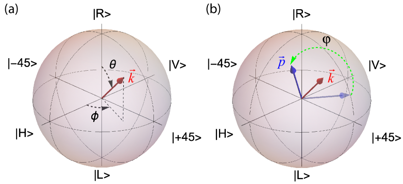
Figure 1: (a) The rotation axis $\vec{k}$ (red) is described in the Bloch sphere by a polar angle $\theta$, and an azimuthal angle $\phi$. Since in our experiments we use the polarization of individual photons as qubits, we take the 1-axis to correspond to $\left|{+45}\right\rangle$, the 2-axis to correspond to $\left|{R}\right\rangle$, and the 3-axis to correspond to $\left|{H}\right\rangle$. (b) A vector that describes the polarization state $\vec{p}$ (blue) is rotated by an angle $\varphi$ about the rotation axis.

As shown in Fig. 1, we define the vector ${\vec{k}(\theta,\phi)}$ to make an angle of $\theta$ from the 2-axis in the Bloch sphere, and its projection onto the plane perpendicular to this axis to make an angle of $\phi$ from the 3-axis . With this convention, $\vec{k}$ is given by

$$\vec{k}=\left({\begin{array}[]{*{20}{c}}{{k_{1}}}\\ {{k_{2}}}\\ {{k_{3}}}\end{array}}\right)=\left({\begin{array}[]{*{20}{c}}{\sin\left({\theta}\right)\sin\left({\phi}\right)}\\ {\cos\left({\theta}\right)}\\ {\sin\left({\theta}\right)\cos\left({\phi}\right)}\end{array}}\right).$$ (3)

Rotations in the Bloch sphere are given by unitary transformations ${{\tilde{U}}_{j}}={\tilde{U}}\left[{{{\vec{k}}(\theta_{j},\phi_{j})},{\varphi_{j}}}\right]$ that are performed between the state preparation and the measurement. Here $j$ labels the device settings, and we use the tilde to denote a 3x3 matrix. This transformation rotates $\vec{p}$ in the Bloch sphere by an angle ${\varphi_{j}}$ about the axis ${\vec{k}(\theta_{j},\phi_{j})}$, and transforms it into $\vec{{p_{j}}^{\prime}}$: $\vec{{p_{j}}^{\prime}}={\tilde{U}}_{j}\vec{p}$. This transformation is equivalent to $\hat{\rho_{j}}^{\prime}=\hat{U_{j}}\hat{\rho}$, where $\hat{U_{j}}$ is the Hilbert-space operator that corresponds to the Bloch-sphere rotation ${\tilde{U}}_{j}$.

After such a transformation, the probability that a photon will be detected on detector 1, $P_{1,j}$, is

$$\begin{split}{P_{1,j}}=&\;{\rm{Tr}}\left({\hat{\Pi}_{1}\hat{\rho_{j}}^{\prime}}\right)\\ =&\;\frac{1}{2}\left[(1+u)+\vec{w}\cdot\vec{{p_{j}}^{\prime}}\right]\\ =&\;\frac{1}{2}\left[(1+u)+\vec{w}\cdot{{\tilde{U}}_{j}}{\vec{p}}\right].\end{split}$$ (4)

Similarly, we have

$${P_{2,j}}=\frac{1}{2}\left[(1-u)-\vec{w}\cdot{{\tilde{U}}_{j}}{\vec{p}}\right].$$ (5)

Assigning a value of $+1$ to a detection at 1 and $-1$ to a detection at 2, we can use Eqs. (4) and (5) to write the expectation value of a measurement as

$$E_{j}=P_{1,j}-P_{2,j}=u+\vec{w}\cdot{{\tilde{U}}_{j}}{\vec{p}}.$$ (6)

To distinguish experimentally measured and theoretically predicted probabilities, we will use $P_{i,j}$ to represent the theoretical probability of detection on detector $i$ for setting $j$ [Eqs. (4) and (5)], and $f_{i,j}$ to represent the corresponding experimentally measured fraction.

II.2 Self-consistent tomography

Our goal is to determine, in a self-consistent manner, the parameters $\vec{p}$, $\vec{w}$ and $u$ that determine the state and the POVMs. They are determined by applying a set of transformations ${\tilde{U}}_{j}$ and experimentally measuring the fractions $f_{i,j}$. An initial solution is obtained by substituting $f_{i,j}$ for $P_{i,j}$ in Eq. (6) and solving for $\vec{p}$, $\vec{w}$ and $u$.

Equation (6) is nonlinear in the components of $\vec{p}$ and $\vec{w}$, but if we define the products of these components as $x_{ij}=p_{i}w_{j}\>(i,j=1,2,3)$ Eq. (6) is linear in $u$ and the nine different $x_{ij}$’s. If we make ten measurements we can solve ten linear equations in these ten unknowns to determine a solution for $u$ and the $x_{ij}$’s. Details of how we do this are given in Appendix B.

As is well described in Ref. [25], self-consistent tomography techniques determine the parameters that describe the state and the measurements to within a choice of gauge. State and measurement operators expressed in different gauges are equivalent, and every observable probability is identical. Each gauge, therefore, corresponds to an arbitrary “reference frame” that one must use to express the operators mathematically [24, 25]. For example, by examining Eqs. (4) and (5) we see that if we simultaneously make the substitutions $\vec{w}\to-\vec{w}$ and $\vec{p}\to-\vec{p}$, the probabilities are unchanged. As such, the two solutions $(\vec{w},\vec{p})$ and $(-\vec{w},-\vec{p})$ are equivalent, but represent different gauges and we must choose one. Physically, what does this choice of gauge represent? Changing the sign of $\vec{p}$, for example, would change the polarization state $\left|H\right\rangle\to\left|V\right\rangle$. For photons this choice of gauge effectively defines what we mean by “horizontal” and “vertical”.

Next, recall that positivity places the constraints $p\leq 1$ and ${w\leq 1-\left|u\right|}$. Furthermore, if ${\tilde{U}}_{1}={\tilde{1}}$, for example, we can rewrite Eq. (6) as $\vec{w}\cdot\vec{p}=wp\cos(\beta)={E_{1}}-u$, where $\beta$ is the angle between $\vec{w}$ and $\vec{p}$. From this we see that the measured expectation values (probabilities) determine the product of the magnitudes of $\vec{p}$ and $\vec{w}$, but cannot determine their individual magnitudes because of a gauge degree of freedom. Physically, this gauge choice trades off between the purity of the state and the discrimination power of the detector. Because of this, in the reconstructions presented below we choose the gauge where ${w=1-\left|u\right|}$, and this choice then determines $p$. This choice is motivated by the design of our experiment, where we expect that the bias parameter is the only thing that degrades the discriminating power of the detector .

The solution to the 10 linear equations, as described in Appendix B, determines $u$, which, given the discussion above, determines $w$ and $p$. What we now need to determine is the directions of $\vec{w}$ and $\vec{p}$. Given the measured values of the $x_{ij}$’s, if we find $p_{i}$, we could determine $w_{j}$ from $w_{j}=x_{ij}/p_{i}$. However, this is problematic if $p_{i}$ is 0, or nearly so. Dividing by $w_{j}$ to find $p_{i}$ is similarly problematic. To avoid this problem, we first find the maximum of the $x_{ij}$’s, which we refer to as

$${\rm{max}}\>x_{ij}=x_{i_{max}j_{max}}=p_{i_{max}}w_{j_{max}}.$$ (7)

With this definition, we can be confident that neither $p_{i_{max}}$ nor $w_{j_{max}}$ are nearly 0. We can then safely write the $w_{j}$’s as

$$w_{j}=\frac{x_{i_{max}j}}{p_{i_{max}}}.$$ (8)

To eliminate the $p_{i}$’s, we can solve these equations to write two of the $w_{j}$’s in terms of the third. For example, suppose that the maximum $x_{ij}$ is $x_{23}$, so $i_{max}=2$ and $j_{max}=3$; then $p_{2}=x_{23}/w_{3}$ and

$$w_{1}=\frac{x_{21}}{x_{23}}w_{3}$$ (9a)

$$w_{2}=\frac{x_{22}}{x_{23}}w_{3}.$$ (9b)

The $w_{3}$ component is used to ensure that the magnitude of $\vec{w}$ is consistent with our choice of gauge, and this determines $\vec{w}$. We can then solve for the components of $\vec{p}$ using

$$p_{i}=\frac{x_{i{j_{max}}}}{w_{j_{max}}}.$$ (10)

This completes the analytic solutions for $u$, $\vec{p}$ and $\vec{w}$. These solutions are used as the initial starting point for a maximum-likelihood solution.

Before moving on, note that there are seven parameters that determine $u$ and the components of $\vec{p}$ and $\vec{w}$. In principle one should be able to find these parameters with only 7 measurements. Indeed, we find that it is possible to do this for most states and POVMs. However, there are certain special cases where a particular set of 7 measurements might not be enough. For example, assume that $\vec{p}=(1,0,0)$ and $\vec{w}=(0,1,0)$. In this case $x_{12}=1$, and all other $x_{ij}$’s are 0. In order to determine $u$ and all the $x_{ij}$’s we need 10 measurements, and with only 7 measurements $x_{12}$ might not be determined. If there are not too many 0’s in the components of $\vec{p}$ or $\vec{w}$ is is possible to determine them with only 7 measurements, but in general we cannot assume that this will be the case.

II.3 Maximum likelihood analysis

The expected probability of measuring a photon on detector $i$ for measurement setting $j$, $P_{i,j}$, is given in Eqs. (4) and (5). The log-likelihood of obtaining a measured fraction of photons on this detector, $f_{i,j}$, is given by

$$L(f,P)={\rm{log}}\;\mathcal{L}(f,P)=\sum\limits_{i,j}f_{i,j}{\rm{log}}(P_{i,j})\;.$$ (11)

Following Ref. [18], we maximize the likelihood function by alternating between QST and QDT. When performing QST we hold the POVM fixed, and the density operator is fixed while performing QDT.

For QST we use the $R\rho R$ method [42, 43]. In this method the density operator at iteration $k+1$ is written in terms of the density operator at iteration $k$ as

$${\hat{\rho}}^{(k+1)}=\hat{R}^{(k)}{\hat{\rho}}^{(k)}\hat{R}^{(k)}\;,$$ (12)

where

$$\hat{R}^{(k)}=\sum\limits_{i,j}\frac{f_{i,j}}{P^{(k)}_{i,j}}\hat{\Pi}_{i,j}\;$$ (13)

and $\hat{\Pi}_{i,j}=\hat{\Pi}_{i}\hat{U}_{j}$. At each iteration the likelihood is guaranteed to increase, and the density operator is guaranteed to remain positive. After each iteration we renormalize the density operator.

For QDT we use the method of Lagrange multipliers described in Refs. [12, 44]. The POVM in iteration $k+1$ is given by

$${\hat{\Pi}}^{(k+1)}_{i}=\hat{R}^{\prime(k)}_{i}{\hat{\Pi}}^{(k)}_{i}\hat{R}^{\prime(k)}_{i},$$ (14)

where

$$\hat{R}^{\prime(k)}_{i}=\sum\limits_{j}\frac{f_{i,j}}{P^{(k)}_{i,j}}\left(\sum\limits_{l}\sum\limits_{m,n}\frac{f_{l,m}}{P^{(k)}_{l,m}}\frac{f_{l,n}}{P^{(k)}_{l,n}}{\hat{\rho}}_{m}{\hat{\Pi}}^{(k)}_{l}{\hat{\rho}}_{n}\right)^{1/2}\hat{\rho}_{j}\;.$$ (15)

Here $\hat{\rho}_{j}=\hat{U}_{j}\hat{\rho}$. Again, the likelihood is guaranteed to increase after each iteration, and the POVM will always be positive.

We use separate termination conditions for QST and QDT, stopping when both conditions are reached. To set the stopping point for QST, we follow the method of Refs. [18, 43]. At each iteration we calculate $S_{\rho}$, which is an upper bound on the difference between the current likelihood and the unknown maximum likelihood

$$\begin{split}L\left({\hat{\rho}}_{ML}\right)-L\left({\hat{\rho}}_{k}\right)\leq&\text{max}\left[\text{eigenvalues}\left(\hat{R}^{(k)}\right)\right]-N\\ =&S_{\rho}.\end{split}$$ (16)

Here ${\hat{\rho}}_{ML}$ is the density operator at maximum likelihood and $N$ is the number of measurements, in our case 10.

To set the stopping point for QDT we use the Frobenius norm of consecutive iterations of the POVM. At each iteration, we calculate

$$\left|\left|{\hat{\Pi}}^{(k)}_{1}-{\hat{\Pi}}^{(k+1)}_{1}\right|\right|=S_{\Pi}.$$ (17)

We stop once both $S_{\rho}$ and $S_{\Pi}$ are less than $10^{-5}$.

It would be possible to use other, possibly more efficient, techniques for maximizing the likelihood. But we have found that the technique we use works well, and is more than efficient enough (the experimental data is acquired in minutes, while the data analysis takes only seconds).

II.4 Figures of merit

To compare the theoretically expected POVM (or state) to that reconstructed by our technique we use the fidelity $F$, which for two POVMs is given by [45, 46]

$$F=\frac{{\left[{{\rm{Tr}}\left({\sqrt{\sqrt{\hat{\Pi}_{1}}\hat{\Pi}_{2}\sqrt{\hat{\Pi}_{1}}}}\right)}\right]^{2}}}{{\rm{Tr}}({\hat{\Pi}_{1}}){\rm{Tr}}({\hat{\Pi}_{2}})}.$$ (18)

The fidelity takes on values $0\leq F\leq 1$ , with $F=1$ corresponding to ${\hat{\Pi}_{1}}={\hat{\Pi}_{2}}$ and $F=0$ corresponding to orthogonal operators. To compare density operators we simply replace $\hat{\Pi}$ by $\hat{\rho}$.

The fidelity is a convenient figure of merit in that it is a measure of how well the measured state agrees with the expected state. However, one needs to trust one’s knowledge of the expected state in order to have confidence in the fidelity. As such, it is also convenient to have a measure that does not depend on explicit knowledge of the expected state. Here we use the total variation distance (TVD) to compare the experimentally measured fractions $f_{i,j}$ to the probabilities returned by the fit to the model, $P_{i,j}$ [47]. The TVD is a measure of how close the measured and modeled probabilities are, and it is given by

$${\rm{TVD}}=\frac{1}{2}\sum\limits_{i,j}|P_{i,j}-f_{i,j}|.$$ (19)

The TVD also has another useful property. Since it depends only on measured and modeled probabilities, and these are independent of the choice of gauge, the TVD is gauge invariant. Any choice of gauge that we make will not affect our determination of the TVD. However, there is no well-motivated measure of fidelity that is gauge invariant [25]. As such, in our experiments we choose between the $(\vec{w},\vec{p})$ and $(-\vec{w},-\vec{p})$ gauges by using the one that maximizes the fidelity with the expected state .

II.5 Larger numbers of qubits

The potential exists for scaling this technique to larger numbers of qubits. An efficient means for doing this is as follows. Imagine a 2-qubit system with two detectors. We can simply use the technique above to perform detector tomography on each of the two detectors, even without knowing the state. This requires 10 measurements to be performed with each detector. We can then use the reconstructed POVMs to perform QST on the source. For a 2-qubit system, QST can be accomplished with as few as 9 measurements [10]. As such, we can self-consistently determine both the unknown state, and both POVMs for a 2-qubit system, with $\sim\!30$ measurements. Due to the gauge degrees of freedom, there are 4 possible state-POVM pairs that describe the system (the continuous gauge degrees of freedom are also still present).

Note, however, that if the source is in a Bell state, for example, the marginal density operator for each individual qubit is a perfectly random mixed state. In this case all of the $x_{ij}$’s are 0, and the technique described above will not work. As such we need to use conditional measurements on one qubit to project the other qubit into a state that is not perfectly random. In this way we can perform detector tomography on each detector. Note that conditional measurements are $only$ needed if the marginal distributions for the one or both of the qubits are perfectly random.

No knowledge of the underlying state is needed here. For example, consider the Bell state

$${|{\phi^{+}}\rangle}=\frac{1}{2}\left({|{H,H}\rangle}+{|{V,V}\rangle}\right).$$ (20)

A measurement of polarization on one of the photons will project it onto some elliptical polarization state ${|{e_{1}}\rangle=a|{H}\rangle+be^{i\phi}|{V}\rangle}$. This projects the other photon into the polarization state ${|{e_{2}}\rangle=a|{H}\rangle+be^{-i\phi}|{V}\rangle}$ via quantum steering. If measurements of the second photon are performed conditionally with the first, the second photon will not be in a random mixed state, and it will be possible to reconstruct both its state and the POVM of the detector that performs measurements on it. If the original beam is in a different Bell state then the second photon will be projected into a different state, but it will always be the case that it will not be in a perfectly random mixed state.

For other more general two-qubit states whose marginals are perfectly random, any conditional measurement that projects the conditionally prepared state into a state that is not perfectly random will suffice. As long as there is some correlation between the qubits, nearly any measurement should accomplish this.

III Experiment

III.1 Apparatus

We use 5 mW of power from a 405 nm, single-frequency laser diode to pump a 25 mm long, type-II, periodically-polled, potassium titanyl phosphate (PPKTP) crystal. This produces spontaneous-parametric-down conversion at 810 nm, and we separate signal and idler beams with a polarizing beam splitter (PBS). The idler beam is focused into a single-mode optical fiber, filtered by a 10 nm bandwidth filter centered at 810 nm, and detected by a single-photon-counting module (SPCM). Detection of an idler photon heralds the production of a coincident, single photon in the signal beam. For coincidence counting we use a coincidence window of 3.2 ns on a commercial time-to-digital converter, and we subtract the expected accidental coincidences.

The signal beam is focused into a single-mode, polarization-preserving optical fiber, and emerges as the “Source” in Fig. 2. Before being detected with SPCMs, signal photons are also filtered with 10 nm bandwidth, 810 nm filters. The heralded signal photons produced by our source have a measured degree of second-order coherence $g^{(2)}(0)=0.024\pm 0.002$, so the signal beam is well described by a single-photon state. Furthermore, by blocking the signal beam we find that the ratio of heralded background detections, including dark counts, to heralded signal-photon detections is 0.0004. As such, we conclude that background detections have a minimal effect on our measurements.

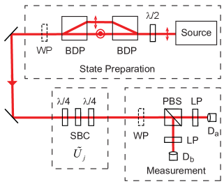
Figure 2: The experimental apparatus. The source consists of heralded single photons emerging from a single-mode optical fiber. BDP denotes a beam-displacing polarizer, $\lambda/2$ denotes a half-wave plate, $\lambda/4$ denotes a quarter-wave plate, WP denotes optional half- and/or quarter-wave plates, SBC denotes a Soleil-Babinet compensator, LP denotes a linear polarizer and PBS denotes a polarizing beam splitter (a Rochon prism). Light emerging from the LPs is wavelength filtered and coupled into multi-mode optical fibers (not shown), which are then coupled to single-photon-counting modules (labeled ${D_{a}}$ and ${D_{b}}$).

Linearly-polarized photons from the source pass through a half-wave plate that rotates their polarization. These photons then pass through a beam-displacing polarizer (BDP) that spatially displaces the horizontal component of the polarization from the vertical component; the fraction of the horizontal and vertical components is adjusted by the rotation angle of the half-wave plate. A second BPD spatially recombines the beams, but the horizontal component is delayed by a time longer than the coherence time of the individual photons. This creates an adjustable mixture of horizontal and vertical polarizations. Half- and/or quarter-wave plates placed after the BDPs allow us to rotate the polarization, and create any state of single-photon polarization. Likewise, half- and/or quarter-wave plates in front of a PBS allow us to perform measurements of any projection of the polarization.

In our data analysis we are able to model the POVMs that describe our detectors in two different ways, and we will present the results separately. In the first model we treat the entire subsystem labeled “Measurement” in Fig. 2 as a two-outcome POVM. We post select on coincident detections between an idler photon, and a signal photon at either $D_{a}$ or $D_{b}$. In this model detection at $D_{a}$ corresponds to ${\hat{\Pi}}_{1}$ and detection at $D_{b}$ corresponds to ${\hat{\Pi}}_{2}$. We exclude events with heralded detections at both $D_{a}$ and $D_{b}$, which are small in number because of our low measured value of $g^{(2)}(0)$. As described above, background events are a small percentage of coincidence detections, so the vast majority of our post-selected events represent true signal-photon detections, and include only a very small number of events where no photons were present at $D_{a}$ or $D_{b}$.

In order to treat the two detectors as corresponding to different operators in a two-outcome POVM, it is necessary for their corresponding values of $u$ and $\vec{w}$ to be the same. The use of a high-quality Rochon PBS (extinction ratio of $>\!10^{4}$ for both polarizations) ensures that the two detectors monitor orthogonal polarizations, thus ensuring that $\vec{w}$ is the same. To ensure that $u$ is the same we need the detection efficiencies to be the same. We do this by inserting linear polarizers after the PBS. These allow us to adjust the amount of light hitting the two detectors, and hence balance their their measured count rates to within $\sim 3\%$. The advantage of this post-selected detector model is that inefficiencies in detection do not effect the POVMs.

In the second model, each detector is assigned its own two-outcome POVM. For example, consider $D_{a}$: ${\hat{\Pi}}_{1}$ corresponds to a coincident detection between the idler detector and $D_{a}$, while ${\hat{\Pi}}_{2}$ corresponds to a heralding detection at the idler detector, but no coincident detection at $D_{a}$. The heralding serves as a “clock” that tells us when to interrogate the detector and observe the outcome. This model has the advantage that we need not assume that the values of $u$ and $\vec{w}$ for $D_{a}$ and $D_{b}$ are the same. The disadvantage is that for our relatively low heralding efficiency, the imbalance $u$ between no detections and detections is large, and dominates the parameters of the POVM.

We use a Soleil-Babinet compensator (SBC) placed between two quarter-wave plates to implement the transformations ${\tilde{U}}\left[{{{\vec{k}}(\theta_{j},\phi_{j})},{\varphi_{j}}}\right]$. The rotation angles of the wave plates and the phase shift of the SBC that make up these transformations are all under computer control. We use the theoretically expected $\tilde{U}_{j}$’s, given the settings of our device, to perform our tomographic reconstructions. Our calibrations, details of which are found in Appendix A, show that all of our $\tilde{U}_{j}$’s have a mean process fidelity of at least 0.994 with the actual experimentally implemented transformation.

To generate the 10 measurements necessary to determine the state and the detector POVMs the computer steps through the transformations and records the singles and coincidence counts. For each measurement setting we acquire approximately 20,000 coincident detections. From the raw counts we calculate the probabilities and expectation values necessary to perform the reconstructions.

III.2 Results

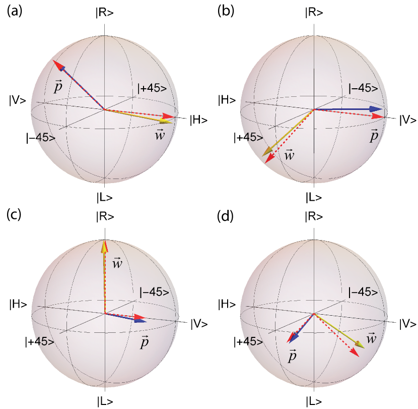
Figure 3: Experimental determinations of the vectors that describe the state $\vec{p}$ (blue) and the POVM $\vec{w}$ (yellow); (a)-(d) show four different experiments. The corresponding theoretically expected vectors are shown as dashed red arrows. The reconstructions here use the first detector model.

Table 1: The data corresponding to the plots in Fig. 3.

Fig.	$\vec{p}$ Expected	$\vec{p}$ Measured	$\vec{w}$ Expected	$\vec{w}$ Measured	$u$ Expected	$u$ Measured
3(a)	$(-1/2,1/\sqrt{2},-1/2)$	$(-0.486,0.697,-0.488)$	$(0,0,1)$	$(0.017,-0.084,0.970)$	0	0.026
3(b)	$(0,0,-1)$	$(0.057,0.117,-0.991)$	$(1/2,-1/\sqrt{2},1/2)$	$(0.487,-0.620,0.553)$	0	0.037
3(c)	$(0,0,-0.6)$	$(-0.076,-0.074,-587)$	$(0,1,0)$	$(0.045,0.998,0.0004)$	0	0.0006
3(d)	$(0.275,-.389,0.275)$	$(0.356,-0.364,0.201)$	$(-1/2,-1/\sqrt{2},-1/2)$	$(-0.571,-0.588,-0.556)$	0	0.009

Table 2: The fidelities and total variation distances corresponding to the data in Fig. 3 and Table 1.

Fig.	Fidelity $\hat{\rho}$	Fidelity ${\hat{\Pi}}_{1}$	Fidelity ${\hat{\Pi}}_{2}$	TVD
3(a)	0.990	0.998	0.998	0.065
3(b)	0.996	0.998	0.998	0.073
3(c)	0.997	0.988	0.999	0.124
3(d)	0.997	0.994	0.994	0.049

We have performed measurements for different states and detector POVMs. Essentially, we place $\vec{p}$ and $\vec{w}$ in different places in the Bloch sphere. We vary the directions of both of these vectors, and we also vary the magnitude of $\vec{p}$ by controlling the purity of the state. We perform five trials for each set of parameters that determine the state and the POVMs. We performed a total of 310 trials.

III.2.1 First detector model

Four example reconstructions are shown in Fig. 3. In this figure we are using the first detector model, in which detection at $D_{a}$ corresponds to ${\hat{\Pi}}_{1}$ and detection at $D_{b}$ corresponds to ${\hat{\Pi}}_{2}$. The theoretically expected, and experimentally determined parameters that describe the state and the POVMs corresponding to those displayed in Fig. 3 are given in Table 1. The theoretically expected parameters are calculated from the known wave-plate settings that determine the state and the measurement.

From the reconstructed state and POVM parameters we can use Eqs. (4) and (5) to calculate the detection probabilities $P_{i,j}$ associated with the model. These and the measured fractions $f_{i,j}$ determine the TVD of the reconstruction using Eq. (19). We can use Eq. (18) to calculate the corresponding fidelities. The TVDs and fidelities corresponding to the entries in Table 1 are given in Table 2.

The fidelities of $\hat{\rho}$ and the ${\hat{\Pi}}_{i}$’s, and the total variation distances of all the trials are shown as histograms in Fig. 4. For the POVMs the fidelities are above 0.99 for 82% of trials, and above 0.98 for 95% of the trials. Fidelities for the density matrices are above 0.99 in 91% of trials, and above 0.98 in 98% of trials. The mean TVD for all trials was found to be $0.11\pm 0.05$. There are 20 terms in the sum of Eq. (19) for the TVD (2 outcomes, 10 measurements), so on average the modeled probabilities and the measured fractions differ by approximately 0.01.

We have estimated our experimental ability to accurately generate the Bloch sphere transformations ${\tilde{U}}\left[{{{\vec{k}}(\theta_{j},\phi_{j})},{\varphi_{j}}}\right]$ by comparing our experimentally measured TVD data to numerically simulated data. We performed simulations while varying the amount of error in the transformation angles, and compared the resulting TVDs to the distribution in Fig. 4(d). The statistics of the errors were assumed to be the same for each of the three angles, having a Gaussian distribution with 0 mean and an adjustable standard deviation. Statistical errors due to finite numbers of counts were also simulated. After performing simulations with differing amounts of error, we find that the distribution of TVDs in the simulations were most similar to those of Fig. 4(d) for a standard deviation of 0.05 radians, and the simulated TVDs in this case are shown in Fig. 5. For this amount of error, the simulated TVD’s had a mean of $0.11\pm 0.04$. The agreement between the simulations and the experiment lead us to believe that the accuracy of our technique is currently limited by errors on the order of 0.05 radians in controlling the angles in the transformations ${\tilde{U}}\left[{{{\vec{k}}(\theta_{j},\phi_{j})},{\varphi_{j}}}\right]$ that we desire . It might be possible to improve our results by applying a neural network or a Bayesian analysis to help us compensate for these errors [28, 50].

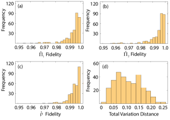
Figure 4: Histograms (a) and (b) show the fidelities of the theoretically expected ${\hat{\Pi}}_{1}$ and ${\hat{\Pi}}_{2}$ with the experimentally determined operators, (c) shows the fidelity of the theoretical and experimental $\hat{\rho}$, and (d) the total variation distance between the measured and the model probability distributions. This data was analyzed using the first detector model.

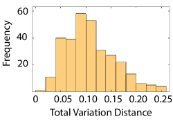
Figure 5: Histogram of TVDs obtained from numerically simulated data, using parameters chosen to align with those of the experimental TVDs displayed in Fig. 4(d).

III.2.2 Second detector model

Table 3: The data for the second detector model, as applied to detector $\rm{D_{b}}$, and corresponding to the same measurements as in TABLE 1.

$\vec{p}$ Expected	$\vec{p}$ Measured	$\vec{w}$ Expected	$\vec{w}$ Measured	$u$ Expected	$u$ Measured
$(-1/2,1/\sqrt{2},-1/2)$	$(-0.482,0.694,-0.482)$	$(0,0,-0.046)$	$(-.001,0.004,-0.046)$	-0.960	-0.954
$(0,0,-1)$	$(0.057,0.089,-0.972)$	$(-0.025,0.035,-0.025)$	$-0.027,0.033-0.028)$	-0.960	-0.949
$(0,0,-0.6)$	$(-0.060,-0.068,-0.558)$	$(0,-0.035,0)$	$(-0.002,-0.035,-0.001)$	-0.960	-0.964
$(0.275,-.389,0.275)$	$(0.329,-0.347,0.194)$	$(0.017,0.023,0.017)$	$(0.020,0.019,0.019)$	-0.960	-0.967

Table 4: The fidelities and total variation distances corresponding to the data in TABLE 3.

Fidelity $\hat{\rho}$	Fidelity ${\hat{\Pi}}_{1}$	Fidelity ${\hat{\Pi}}_{2}$	TVD
0.986	0.998	0.999996	0.0042
0.986	0.999	0.999991	0.0066
0.997	0.999	0.999998	0.0030
0.997	0.993	0.999675	0.0029

In the second detector model each detector is treated separately, and the two-outcome POVMs correspond to heralded detections ${\hat{\Pi}}_{1}$ or no detections ${\hat{\Pi}}_{2}$ for each detector. We use the same experimental data as was used in the first detector model, we just analyze it differently.

Expected and reconstructed state and measurement parameters for detector $D_{b}$ are shown in Table 3 (all results for detector $D_{a}$ are very similar to those of $D_{b}$), while Table 4 shows the measured fidelities and TVDs corresponding to this data. Each row of Table 3 corresponds to an analysis of the same data used to construct the corresponding row of Table 1. The primary difference between the two models is the imbalance parameter $u$. The first model is insensitive to the heralding efficiency, while the second model is sensitive to it. The heralding efficiency is equal to $1-|u|$, and we see that the data in Table 3 reflect an overall heralding efficiency of 3-5%, which is consistent with independent measurements of this parameter. We measure this efficiency by dividing the total number of signal-idler coincidence detections by the total number of idler (heralding beam) detections . We find that the efficiency fluctuates slightly from day to day as the fiber-coupling of the source changes. The low efficiency is primarily due to the fact that we have not optimized the coupling of our source into the single-mode fibers.

In Table 3 the theoretically expected parameters that describe $\vec{p}$ and $\vec{w}$ are calculated from the known wave-plate settings that determine the state and the measurement. We use an expected value for the bias parameter of $u=-0.96$, corresponding to a heralding efficiency of 4%, which is consistent with our measured efficiencies. We note that the fidelities are not particularly sensitive to changes in the expected value of $u$. If this value is varied between $-0.93$ and $-0.98$, the fidelities for ${\hat{\Pi}}_{1}$ in Table 4 are unchanged, while those of ${\hat{\Pi}}_{2}$ remain above 0.999.

Fig. 6 shows histograms of the measured fidelities and TVDs corresponding to all of the trials. One thing to note is that despite the relatively low heralding efficiency, the reconstruction of the density operator is nearly as good here as it was for the first detector model. The fidelity of $\hat{\rho}$ is over 0.99 for 76% of the trials, and over 0.98 for 92% of trials.

The fidelities for the POVMs are better for the second detector model than they were for the first. For ${\hat{\Pi}}_{1}$ the fidelities exceed 0.99 for 89% of the trials, and 0.98 for 97% of trials. For ${\hat{\Pi}}_{2}$ the lowest fidelity is 0.999424. Clearly the large imbalance is having a strong effect on the fidelities of ${\hat{\Pi}}_{2}$. With $u\approx-1$, ${\hat{\Pi}}_{2}$ is approximately equal to the identity operator and is largely independent of $\vec{w}$.

Finally, the TVDs for the second detector model have an average value of $0.006\pm 0.003$, so the model fits the data quite well. Note that this measure is independent of any assumptions about the theoretically expected state or POVMs. In particular, it is independent of the expected value of $u$.

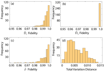
Figure 6: Histograms (a) and (b) show the fidelities of the theoretically expected ${\hat{\Pi}}_{1}$ and ${\hat{\Pi}}_{2}$ with the experimentally determined operators, (c) shows the fidelity of the theoretical and experimental $\hat{\rho}$, and (d) the total variation distance between the measured and the model probability distributions. This data was analyzed using the second detector model, as applied to $\rm{D_{b}}$.

III.2.3 Discussion of the models

Recall that the first detector model treats the apparatus in the box labeled “Measurement” in Fig. 2 as a single, two-outcome POVM. The advantage of this model is that because the detections are post selected, it is insensitive the heralding efficiency of the single-photon detections. For this model to be valid, it is necessary for $u$ and $\vec{w}$ to be the same for both $D_{a}$ and $D_{b}$. Important contributors to these parameters are the detector efficiencies, and the ability of the PBS to accurately separate orthogonally polarized photons.

If the detection apparatus does not satisfy these conditions, it is necessary to use the second detector model and determine separate POVMs for $D_{a}$ and $D_{b}$. In our experiments the low heralding efficiency meant that there was a significant bias toward no detections, so the no-detection measurement operator was nearly equal to the identity operator, and hence largely independent of the measurement parameters. The fidelity of the operator corresponding to a detection was found to be somewhat insensitive to changes in the expected value of $u$, and hence to changes in the expected $w$. Thus, if the detection efficiency is low, one should be aware of these limitations in the reconstructed POVMs. This problem would be reduced or eliminated in the case of higher detection efficiencies. Despite these issues, the polarization state is reconstructed with high fidelity, so one can still have high confidence in it, even with low efficiency detection.

IV Conclusions

We have described a technique which is capable of estimating both the unknown quantum state of a single qubit, and a two-outcome POVM that performs measurements of this qubit, in a self-consistent manner. This is done by performing a series of known, unitary transformations between the state preparation and measurement stages. This technique makes minimal assumptions about the state and the POVMs. We present two different models for the POVMs. In one model we assume that the $u$ and $\vec{w}$ parameters of the two detectors are the same, but in the other we do not need this assumption.

We assume that the unitary transformations are known. In our experiments this assumption is valid because the transformations are characterized classically with high fidelity, as demonstrated in Appendix A. While our assumption will not be valid in all experiments, it will be valid in many optical experiments where the transformations can be calibrated classically [31, 32, 33]. Knowing these transformations is what allows us to self-consistently determine the state and the POVMs with only ten measurements. This saves time when compared to other techniques that do not assume the transformations are known, but require approximately 50 measurements [25, 24].

We have experimentally implemented this technique, and applied it to a system described by the polarization of individual photons. We find that the technique works quite well, as the fidelities between expected and measured density operators and POVMs are found to exceed 0.98 for at least 92% of our 310 experimental trials.

Appendix A Polarization transformations

Here we describe our apparatus that generates rotations $\tilde{U}\left[{{{\vec{k}}\left(\theta,\phi\right)},{\varphi}}\right]$ in the Bloch sphere for polarization qubits. We describe the theory behind the design of our device that implements these general polarization transformations [52, 53, 54], and present experimental results that demonstrate its performance.

A.1 Theory

Polarization transformations that do not modify the total intensity are unitary transformations, and may be represented by 3x3 matrices. As seen in Fig. 1, a general polarization transformation is represented in the Bloch sphere by a rotation ${\tilde{R}}\left({\theta,\phi,\varphi}\right)$, having a rotation axis $\vec{k}$ and a rotation angle $\varphi$. The rotation axis is parameterized by two angles, $\theta$ and $\phi$.

As seen in Fig. 1, we take the rotation axis ${\vec{k}}$ to make an angle of $\theta$ from the 2-axis ($\left|R\right\rangle$) in the Bloch sphere, and its projection onto the plane perpendicular to this axis to make an angle of $\phi$ from the 3-axis ($\left|H\right\rangle$). With this convention, the rotation axis is given by Eq. (3).

If we define $c=\cos\left({\varphi}\right)$, $d=1-\cos\left({\varphi}\right)$, $s=\sin\left({\varphi}\right)$, we can express ${\tilde{R}}\left({\theta,\phi,\varphi}\right)$ in matrix form as

$$\tilde{R}\left({\theta,\phi,\varphi}\right)=$$

$$\left({\begin{array}[]{*{20}{c}}{dk_{1}^{2}+c}&{d{k_{1}}{k_{2}}-s{k_{3}}}&{d{k_{3}}{k_{1}}+s{k_{2}}}\\ {d{k_{1}}{k_{2}}+s{k_{3}}}&{dk_{2}^{2}+c}&{d{k_{3}}{k_{2}}-s{k_{1}}}\\ {d{k_{3}}{k_{1}}-s{k_{2}}}&{d{k_{3}}{k_{2}}+s{k_{1}}}&{dk_{3}^{2}+c}\end{array}}\right).$$ (24)

Furthermore, let $R_{ij}$ be the element in the $i^{th}$ row and $j^{th}$ column of matrix $\tilde{R}$. Given a 3x3 unitary matrix that represents a rotation, we can extract the rotation angle and rotation axis using [55]

$$\cos\left({\varphi}\right)=\frac{1}{2}\left[{{\rm{Tr}}\left({\tilde{R}}\right)-1}\right]$$ (25a)

$${k_{1}}=\frac{1}{{2\sin\left({\varphi}\right)}}\left({{R_{32}}-{R_{23}}}\right)$$ (25b)

$${k_{2}}=\frac{1}{{2\sin\left({\varphi}\right)}}\left({{R_{13}}-{R_{31}}}\right)$$ (25c)

$${k_{3}}=\frac{1}{{2\sin\left({\varphi}\right)}}\left({{R_{21}}-{R_{12}}}\right).$$ (25d)

We wish to implement general polarization transformations, described by Eq. (24), using wave plates. Consider a wave plate that has a phase shift $\phi_{W}$ between its fast and slow axes, and whose fast-axis is rotated by $\theta_{W}$ from the horizontal. If we define $c^{\prime}=\cos\left({2\theta_{W}}\right)$ and $s^{\prime}=\sin\left({2\theta_{W}}\right)$, the transformation matrix that describes this wave plate can be written as [56]

$$\tilde{M}\left({\theta_{W},\phi_{W}}\right)=$$

$$\left({\begin{array}[]{*{20}{c}}{{{s^{\prime}}^{2}}+{{c^{\prime}}^{2}}\cos\left(\phi_{W}\right)}&{-c^{\prime}\sin\left(\phi_{W}\right)}&{c^{\prime}s^{\prime}\left[{1-\cos\left(\phi_{W}\right)}\right]}\\ {c^{\prime}\sin\left(\phi_{W}\right)}&{\cos\left(\phi_{W}\right)}&{-s^{\prime}\sin\left(\phi_{W}\right)}\\ {c^{\prime}s^{\prime}\left[{1-\cos\left(\phi_{W}\right)}\right]}&{s^{\prime}\sin\left(\phi_{W}\right)}&{{{c^{\prime}}^{2}}+{{s^{\prime}}^{2}}\cos\left(\phi_{W}\right)}\end{array}}\right).$$ (29)

A special case that is of interest to us is the matrix that corresponds to a quarter-wave plate, ${\tilde{M}_{Q}}\left(\theta_{W}\right)=\tilde{M}\left({\theta_{W},\phi_{W}=\pi/2}\right)$.

The wave plate implementation of a general polarization transformation that we use is given by

$$\tilde{R}\left({\theta,\phi,\varphi}\right)=$$

$${\tilde{M}_{Q}}\left({\frac{{\phi}}{2}}\right)\tilde{M}\left[{\frac{\pi}{4}+\frac{1}{2}\left({\phi-\theta}\right),\varphi}\right]{\tilde{M}_{Q}}\left({\frac{{\phi}}{2}+\frac{\pi}{2}}\right).$$ (30)

Multiplying the matrices to the right of the equal sign in Eq. (30), and applying Eq. (25) to the resulting matrix, verifies that this combination of wave plates does indeed implement $\tilde{R}\left({\theta,\phi,\varphi}\right)$. Physically, this corresponds to a variable-wave plate placed between two quarter-wave plates. From Eq. (30) we find that the phase shift of the variable-wave plate must be equal to the rotation angle in the Bloch sphere, $\phi_{W}=\varphi$, and its rotation angle must be

$${\theta_{W}}=\frac{\pi}{4}+\frac{1}{2}\left({\phi-\theta}\right).$$ (31)

The rotation angle of the second quarter-wave plate is ${\theta_{Q}}={\phi}/{2}$ , while the rotation angle of the first is $\theta_{Q}+\pi/2$.

A.2 Process Fidelity

We verify the operation of our device by inputting classical light of known polarization into it, and measuring three of the Stokes parameters of the light that emerges from it. (The fourth Stokes parameter is the total intensity, and we normalize this to 1.) The classical Stokes parameters are equivalent to the parameters of the vector $\vec{p}$ that we use to describe the quantum state of polarization (although the numbering scheme for the two is different: $p_{1}=S_{2}$, $p_{2}=S_{3}$ and $p_{3}=S_{1}$).

We wish to determine the “classical fidelity” of our transformations. Note that the theoretically expected Stokes vectors in our experiment are “pure”: they have unit magnitude. If one of the states is pure, the quantum fidelity of Eq. (18) can be simplified to [57]

$${F}={\rm Tr}({\hat{\rho}}_{1}{\hat{\rho}}_{2}).$$ (32)

Using Eq. (1), it is straightforward to demonstrate that we can rewrite this expression in terms of the vectors that describe the states as

$${F}=\frac{1}{2}(1+{\vec{p}}_{1}\cdot{\vec{p}}_{2}).$$ (33)

As such, we take the classical fidelity to be given by Eq. (33), where ${\vec{p}}_{1}$ and ${\vec{p}}_{2}$ are the Stokes vectors of the expected and measured polarizations. The fidelity of the entire process that describes the transformation is given by the fidelity between the measured output state and the theoretically expected output state, averaged over many states [15, 58].

A.3 Experiment

Our experimental apparatus is depicted in Fig. 7. The light source is an 808nm laser diode, coupled to a polarization-preserving, single-mode fiber, which acts as a spatial filter. We prepare the polarization that we input to our device by rotating a linear polarizer and a quarter-wave plate. A half-wave plate preceding the linear polarizer allows us to adjust the intensity. The beam passes through our unitary-transformation apparatus, and the polarization emerging from it is analyzed by a commercial polarimeter (Thorlabs PAX1000IR1).

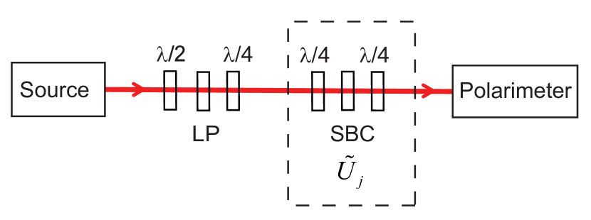
Figure 7: The experimental apparatus for characterizing our device that implements ${\tilde{U}}_{j}$. The source is a laser diode coupled to a single-mode optical fiber. Here LP denotes a linear polarizer, SBC denotes a Soleil-Babinet compensator, $\lambda/2$ denotes a half-wave plate and $\lambda/4$ denotes a quarter-wave plate. The two quarter-wave plates on either side of the SBC are Berek compensators that have been adjusted for $\lambda/4$ retardation.

To illustrate how our device implements general polarization transformations, we perform a series of measurements. We begin by fixing the rotation angles of the wave plates in our device that implements ${\tilde{U}}_{j}$, which fixes the rotation axis in the Bloch sphere. Next we fix the input polarization by setting the rotation angles of the linear polarizer and quarter-wave plate that follow our source. Now we scan the phase shift of the SBC (which scans the rotation angle) in 17 equally-spaced steps that range from 0 to $2\pi$ inclusive, while measuring the normalized Stokes vectors of the output polarization. These vectors should form a “ring” around the rotation axis. We can now vary the input polarization, and repeat the sequence of measurements described above to sweep out another ring. In order to obtain reproducible results, the rotation axes of the three wave plates that make up our device are controlled by computer via stepper motors. The phase shift of the SBC is also computer controlled using a DC servo motor.

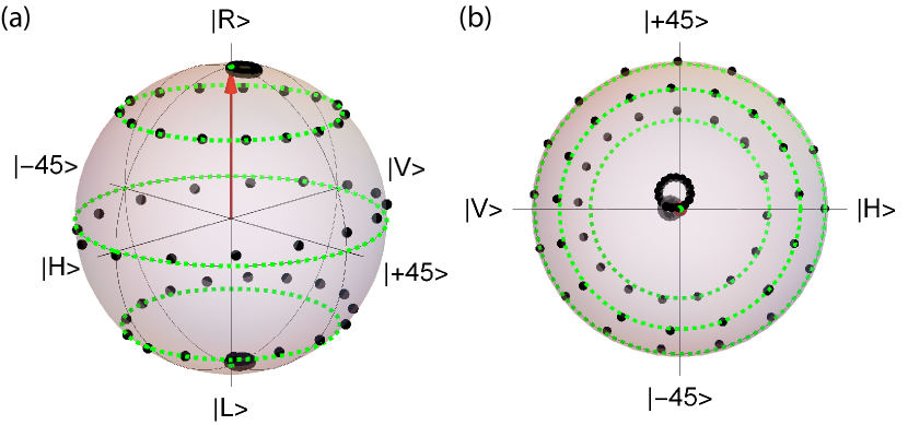
Figure 8: Experimentally measured Stokes vectors (black dots) and corresponding theoretical predictions (green lines). The rotation axis is shown as a red arrow. (a) is a side view of the Bloch sphere, while (b) shows a view looking down along the rotation axis.

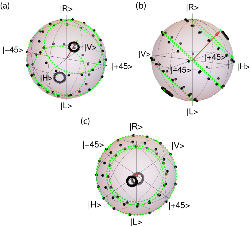
Figure 9: Experimentally measured Stokes vectors (black dots) and corresponding theoretical predictions (green lines). The rotation axis is shown as a red arrow. (a) and (b) are side views of the Bloch sphere, while (c) shows a view looking down along the rotation axis.

Figure 8 shows the result of measurements performed with our device set to perform a rotation about the $\left|R\right\rangle$ axis. In this figure there are 5 different input polarizations, so there are 5 rings. The black dots show the experimentally measured Stokes vectors, while the green lines represent the theoretical predictions. Figure 9 shows the same thing, but for a rotation axis given by the angles $\theta=\phi=\pi/4$. As expected, the experimental Stokes vectors all lie near the surface of the Bloch sphere, which means that the measured polarization states are nearly pure. The experimental points lie near the theoretical curves, indicating at least qualitative agreement between the theory and the experiments.

To verify that the agreement is quantitative, we can compute process fidelities from our measurements. The data from the transformation displayed in Fig. 8 yield an average process fidelity of $F=0.997\pm 0.002$. For the data depicted in Fig. 9 we find $F=0.994\pm 0.005$. The transformations that we use in our experiments are listed in Table 5. We have determined the fidelities for each of these and find that the mean process fidelity between the theoretically expected and corresponding measured transformation is at least 0.994. These fidelities are similar with those that we obtained for the quantum density operators (e.g., Fig. 4). These measurements are thus consistent with the idea that the thing that currently limits the precision of our measurements is our ability to control the unitary transformations.

In the tomographic reconstructions of Sec. 3.B we use the theoretically expected ${\tilde{U}}_{j}$’s of Table 5. We do this because it is these transformations that yield the linear inversion of Eq. (35), given below. It might be possible in the future to perform some form of “classical process tomography” from our classical calibration data to yield maximum likely descriptions of our transformations, and this might improve our results. But, as stated above, the theoretical transformations we use in our reconstructions have a process fidelity of at least 0.994 with the measured transformations, so a full process tomography determination of the ${\tilde{U}}_{j}$’s cannot yield transformations that are significantly more accurate than the ones we use.

To ensure that the classical calibration we perform here is still valid for the quantum experiments, the apparatus labeled ${\tilde{U}}_{j}$ in Fig. 7 is left in place, and the beam path is defined with irises. The polarization preparation is then replaced by the single-photon state preparation apparatus in Fig. 2, which is mode-matched into the irises. The polarimeter is replaced by the measurement apparatus in Fig. 2

Appendix B Linear equations

Table 5: The ten unitary transformations that we use in our experiments.

${\tilde{U}}_{j}$	$\theta_{j}$	$\phi_{j}$	$\varphi_{j}$
${\tilde{U}}_{1}$	0	0	0
${\tilde{U}}_{2}$	0	0	$\pi/2$
${\tilde{U}}_{3}$	0	0	$\pi$
${\tilde{U}}_{4}$	$\pi/2$	0	$\pi$
${\tilde{U}}_{5}$	$\pi/2$	0	$\pi/2$
${\tilde{U}}_{6}$	$\pi/2$	$\pi/2$	$\pi/2$
${\tilde{U}}_{7}$	$\pi/2$	$\pi/2$	$\pi$
${\tilde{U}}_{8}$	$\pi/2$	$\pi/4$	$\pi$
${\tilde{U}}_{9}$	$\pi/4$	0	$\pi$
${\tilde{U}}_{10}$	$\pi/4$	$\pi/2$	$\pi$

Here we describe our solutions to the set of linear equations.

The ten Block-sphere rotations that we use for our measurements are listed in Table 5. Substituting these into Eq. (6) yields

$$u+p_{1}w_{1}+p_{2}w_{2}+p_{3}w_{3}=E_{1}$$ (34a)

$$u+p_{3}w_{1}+p_{2}w_{2}-p_{1}w_{3}=E_{2}$$ (34b)

$$u-p_{1}w_{1}+p_{2}w_{2}-p_{3}w_{3}=E_{3}$$ (34c)

$$u-p_{1}w_{1}-p_{2}w_{2}+p_{3}w_{3}=E_{4}$$ (34d)

$$u-p_{2}w_{1}+p_{1}w_{2}+p_{3}w_{3}=E_{5}$$ (34e)

$$u+p_{1}w_{1}-p_{3}w_{2}+p_{2}w_{3}=E_{6}$$ (34f)

$$u+p_{1}w_{1}-p_{2}w_{2}-p_{3}w_{3}=E_{7}$$ (34g)

$$u+p_{3}w_{1}-p_{2}w_{2}+p_{1}w_{3}=E_{8}$$ (34h)

$$u-p_{1}w_{1}+p_{3}w_{2}+p_{2}w_{3}=E_{9}$$ (34i)

$$u+p_{2}w_{1}+p_{1}w_{2}-p_{3}w_{3}=E_{10}.$$ (34j)

Substituting $x_{ij}=p_{i}w_{j}$ into Eq. (34), we see that Eq. (34) represents a set of 10 linear equations in 10 unknowns $u,x_{ij}\>(i,j=1,2,3)$. Solving them yields

$$u=\frac{1}{4}(E_{1}+E_{3}+E_{4}+E_{7})$$ (35a)

$$x_{11}=\frac{1}{4}(E_{1}-E_{3}-E_{4}+E_{7})$$ (35b)

$$x_{12}=\frac{1}{4}(-E_{1}-E_{3}-E_{4}+2E_{5}-E_{7}+2E_{10})$$ (35c)

$$x_{13}=\frac{1}{4}(E_{1}-2E_{2}+E_{3}-E_{4}-E_{7}+2E_{8}).$$ (35d)

$$x_{21}=\frac{1}{4}(E_{1}-E_{3}+E_{4}-2E_{5}-E_{7}+2E_{10}).$$ (35e)

$$x_{22}=\frac{1}{4}(E_{1}+E_{3}-E_{4}-E_{7}).$$ (35f)

$$x_{23}=\frac{1}{4}(-E_{1}-E_{3}-E_{4}+2E_{6}-E_{7}+2E_{9}).$$ (35g)

$$x_{31}=\frac{1}{4}(-E_{1}+2E_{2}-E_{3}-E_{4}-E_{7}+2E_{8}).$$ (35h)

$$x_{32}=\frac{1}{4}(E_{1}-E_{3}-E_{4}-2E_{6}+E_{7}+2E_{9}).$$ (35i)

$$x_{33}=\frac{1}{4}(E_{1}-E_{3}+E_{4}-E_{7}).$$ (35j)

Thus, performing measurements of expectation values with the settings given in Table 5 and using Eq. (35) yields values for the quantities $u$, $x_{ij}$.

Note that the settings given in Table 5 are not unique. Any ten settings that yield linearly independent equations for the expectation values [Eq. (34)] will allow us to solve for $u$ and the $x_{ij}$’s. We have chosen these particular settings because the solutions in this case [Eq. (35)] are fairly simple.

References

- Blume-Kohout et al. [2017] R. Blume-Kohout, J. K. Gamble, E. Nielsen, K. Rudinger, J. Mizrahi, K. Fortier, and P. Maunz, Demonstration of qubit operations below a rigorous fault tolerance threshold with gate set tomography, Nat. Commun. 8, 14485 (2017).
- Hughes et al. [2020] A. C. Hughes, V. M. Schafer, K. Thirumalai, D. P. Nadlinger, S. R. Woodrow, D. M. Lucas, and C. J. Ballance, Benchmarking a High-Fidelity Mixed-Species Entangling Gate, Phys. Rev. Lett. 125, 080504 (2020).
- Feldman et al. [2018] M. E. Feldman, G. K. Juul, S. J. van Enk, and M. Beck, Loop state-preparation-and-measurement tomography of a two-qubit system, J. Opt. Soc. Am. B 35, 1811 (2018).
- Moore and van Enk [2020] I. D. Moore and S. J. van Enk, Self-consistent tomography and measurement-device independent cryptography, (2020), arXiv:2006.06559 [quant-ph] .
- Coleman et al. [2020] M. R. Coleman, K. G. Ingalls, J. T. Kavulich, S. J. Kemmerly, N. C. Salinas, E. V. Ramirez, and M. Schlosshauer, Parity-based, bias-free optical quantum random number generation with min-entropy estimation, J. Opt. Soc. Am. B 37, 2088 (2020).
- Seiler et al. [2020] J. Seiler, T. Strohm, and W. P. Schleich, Estimating the privacy of quantum-random numbers, New J. Phys. 22, 093063 (2020).
- Vogel and Risken [1989] K. Vogel and H. Risken, Determination of quasiprobability distributions in terms of probability distributions for the rotated quadrature phase, Phys. Rev. A 40, R2847 (1989).
- Smithey et al. [1993] D. T. Smithey, M. Beck, M. G. Raymer, and A. Faridani, Measurement of the Wigner distribution and the density matrix of a light mode using optical homodyne tomography: Application to squeezed states and the vacuum, Phys. Rev. Lett. 70, 1244 (1993).
- Leonhardt [1997] U. Leonhardt, Measuring the Quantum State of Light (Cambridge University Press, Cambridge, UK, 1997).
- Altepeter et al. [2006] J. B. Altepeter, E. R. Jeffrey, and P. G. Kwiat, Photonic state tomography, in Advances in Atomic, Molecular and Optical Physics, Vol. 52, edited by P. R. Berman and C. C. Lin (Elsevier, Amsterdam, 2006) pp. 105–159.
- Luis and Sanchez-Soto [1999] A. Luis and L. L. Sanchez-Soto, Complete characterization of arbitrary quantum measurement processes, Phys. Rev. Lett. 83, 3573 (1999).
- Fiurášek [2001] J. Fiurášek, Maximum-likelihood estimation of quantum measurement, Phys. Rev. A 64, 024102 (2001).
- Lundeen et al. [2009] J. S. Lundeen, A. Feito, H. Coldenstrodt-Ronge, K. L. Pregnell, C. Silberhorn, T. C. Ralph, J. Eisert, M. B. Plenio, and I. A. Walmsley, Tomography of quantum detectors, Nat. Phys. 5, 27 (2009).
- Chuang and Nielsen [1997] I. L. Chuang and M. A. Nielsen, Prescription for experimental determination of the dynamics of a quantum black box, J. Mod. Opt. 44, 2455 (1997).
- Poyatos et al. [1997] J. F. Poyatos, J. I. Cirac, and P. Zoller, Complete characterization of a quantum process: The two-bit quantum gate, Phys. Rev. Lett. 78, 390 (1997).
- D’Ariano and Lo Presti [2004] G. M. D’Ariano and P. Lo Presti, Characterization of quantum devices, in Quantum State Estimation, Lecture Notes in Physics, Vol. 649, edited by M. G. A. Paris and J. Rehacek (Springer-Verlag, Berlin, 2004) pp. 297–332.
- Medford et al. [2013] J. Medford, J. Beil, J. M. Taylor, S. D. Bartlett, A. C. Doherty, E. I. Rashba, D. P. DiVincenzo, H. Lu, A. C. Gossard, and C. M. Marcus, Self-consistent measurement and state tomography of an exchange-only spin qubit, Nat. Nanotechnol. 8, 654 (2013).
- Keith et al. [2018] A. C. Keith, C. H. Baldwin, S. Glancy, and E. Knill, Joint quantum-state and measurement tomography with incomplete measurements, Phys. Rev. A 98, 042318 (2018).
- Řeháček et al. [2010] J. Řeháček, D. Mogilevtsev, and Z. Hradil, Operational tomography: Fitting of data patterns, Phys. Rev. Lett. 105, 010402 (2010).
- Mogilevtsev et al. [2013] D. Mogilevtsev, A. Ignatenko, A. Maloshtan, B. Stoklasa, J. Řeháček, and Z. Hradil, Data pattern tomography: Reconstruction with an unknown apparatus, New J. Phys. 15, 025038 (2013).
- Cooper et al. [2014] M. Cooper, M. Karpiński, and B. J. Smith, Local mapping of detector response for reliable quantum state estimation, Nat. Commun. 5, 4332 (2014).
- Mogilevtsev et al. [2012] D. Mogilevtsev, J. Řeháček, and Z. Hradil, Self-calibration for self-consistent tomography, New J. Phys. 14, 095001 (2012).
- Stark [2014] C. Stark, Self-consistent tomography of the state-measurement Gram matrix, Phys. Rev. A 89, 052109 (2014).
- Zhang et al. [2020] A. Zhang, J. Xie, H. Xu, K. Zheng, H. Zhang, Y.-T. Poon, V. Vedral, and L. Zhang, Experimental Self-Characterization of Quantum Measurements, Phys. Rev. Lett. 124, 040402 (2020).
- Blume-Kohout et al. [2013] R. Blume-Kohout, J. K. Gamble, E. Nielsen, J. Mizrahi, J. D. Sterk, and P. Maunz, Robust, self-consistent, closed-form tomography of quantum logic gates on a trapped ion qubit, (2013), arXiv:1310.4492 [quant-ph] .
- Dehollain et al. [2016] J. P. Dehollain, J. T. Muhonen, R. Blume-Kohout, K. M. Rudinger, J. K. Gamble, E. Nielsen, A. Laucht, S. Simmons, R. Kalra, A. S. Dzurak, and A. Morello, Optimization of a solid-state electron spin qubit using gate set tomography, New J. Phys. 18, 103018 (2016).
- Nielsen et al. [2020] E. Nielsen, J. K. Gamble, K. Rudinger, T. Scholten, K. Young, and R. Blume-Kohout, Gate Set Tomography, (2020), arXiv:2009.07301 [quant-ph] .
- Di Matteo et al. [2020] O. Di Matteo, J. Gamble, C. Granade, K. Rudinger, and N. Wiebe, Operational, gauge-free quantum tomography, Quantum 4, 364 (2020).
- Reck et al. [1994] M. Reck, A. Zeilinger, H. J. Bernstein, and P. Bertani, Experimental realization of any discrete unitary operator, Phys. Rev. Lett. 73, 58 (1994).
- Clements et al. [2016] W. R. Clements, P. C. Humphreys, B. J. Metcalf, W. S. Kolthammer, and I. A. Walmsley, Optimal design for universal multiport interferometers, Optica 3, 1460 (2016).
- Carolan et al. [2015] J. Carolan, C. Harrold, C. Sparrow, E. Martín-López, N. J. Russell, J. W. Silverstone, P. J. Shadbolt, N. Matsuda, M. Oguma, M. Itoh, G. D. Marshall, M. G. Thompson, J. C. F. Matthews, T. Hashimoto, J. L. O’Brien, and A. Laing, Universal linear optics, Science 349, 711 (2015).
- Mennea et al. [2018] P. L. Mennea, W. R. Clements, D. H. Smith, J. C. Gates, B. J. Metcalf, R. H. S. Bannerman, R. Burgwal, J. J. Renema, W. S. Kolthammer, I. A. Walmsley, and P. G. R. Smith, Modular linear optical circuits, Optica 5, 1087 (2018).
- Flamini et al. [2018] F. Flamini, N. Spagnolo, and F. Sciarrino, Photonic quantum information processing: A review, Rep. Prog. Phys. 82, 016001 (2018).
- Spring et al. [2013] J. B. Spring, B. J. Metcalf, P. C. Humphreys, W. S. Kolthammer, X. M. Jin, M. Barbieri, A. Datta, N. Thomas-Peter, N. K. Langford, D. Kundys, J. C. Gates, B. J. Smith, P. G. R. Smith, and I. A. Walmsley, Boson sampling on a photonic chip, Science 339, 798 (2013).
- Metcalf et al. [2014] B. J. Metcalf, J. B. Spring, P. C. Humphreys, N. Thomas-Peter, M. Barbieri, W. S. Kolthammer, X.-M. Jin, N. K. Langford, D. Kundys, J. C. Gates, B. J. Smith, P. G. R. Smith, and I. A. Walmsley, Quantum teleportation on a photonic chip, Nat. Photon. 8, 770 (2014).
- Gräfe et al. [2014] M. Gräfe, R. Heilmann, A. Perez-Leija, R. Keil, F. Dreisow, M. Heinrich, H. Moya-Cessa, S. Nolte, D. N. Christodoulides, and A. Szameit, On-chip generation of high-order single-photon W-states, Nat. Photon. 8, 791 (2014).
- Sparrow et al. [2018] C. Sparrow, E. Martín-López, N. Maraviglia, A. Neville, C. Harrold, J. Carolan, Y. N. Joglekar, T. Hashimoto, N. Matsuda, J. L. O’Brien, D. P. Tew, and A. Laing, Simulating the vibrational quantum dynamics of molecules using photonics, Nature 557, 660 (2018).
- Guan et al. [2019] J. Guan, A. J. Menssen, X. Liu, J. Wang, and M. J. Booth, Component-wise testing of laser-written integrated coupled-mode beam splitters, Opt. Lett. 44, 3174 (2019).
- Jackson and van Enk [2015] C. Jackson and S. J. van Enk, Detecting correlated errors in state-preparation-and-measurement tomography, Phys. Rev. A 92, 042312 (2015).
- Note [1] We define our angles in this way because in our experiments we use qubits based on photon polarization, which is more often depicted in the Poincaré sphere. In this case the 1-axis corresponds to +45-degree linear polarization, the 2-axis corresponds to right-circular polarization and the 3-axis corresponds to horizontal polarization.
- Note [2] If we were using a Bayesian analysis, we would incorporate this a priori information into the Bayesian prior distribution [28].
- Řeháček et al. [2007] J. Řeháček, Z. Hradil, E. Knill, and A. I. Lvovsky, Diluted maximum-likelihood algorithm for quantum tomography, Phys. Rev. A 75, 042108 (2007).
- Glancy et al. [2012] S. Glancy, E. Knill, and M. Girard, Gradient-based stopping rules for maximum-likelihood quantum-state tomography, New J. Phys. 14, 095017 (2012).
- Chen et al. [2019] Y. Chen, M. Farahzad, S. Yoo, and T.-C. Wei, Detector tomography on IBM quantum computers and mitigation of an imperfect measurement, Phys. Rev. A 100, 052315 (2019).
- Jozsa [1994] R. Jozsa, Fidelity for Mixed Quantum States, J. Mod. Opt. 41, 2315 (1994).
- Zhang et al. [2012] L. Zhang, A. Datta, H. B. Coldenstrodt-Ronge, X.-M. Jin, J. Eisert, M. B. Plenio, and I. A. Walmsley, Recursive quantum detector tomography, New Journal of Physics 14, 115005 (2012).
- Rudinger et al. [2019] K. Rudinger, T. Proctor, D. Langharst, M. Sarovar, K. Young, and R. Blume-Kohout, Probing Context-Dependent Errors in Quantum Processors, Phys. Rev. X 9, 021045 (2019).
- Note [3] For this particular gauge degree of freedom, where we have only two possible gauges to chose from, and fixing the gauge is only necessary to calculate the fidelity, we find that maximizing the fidelity works sufficiently well.
- Note [4] The calibration of the unitary transformations presented in Appendix A yields fidelities consistent with those of Fig. 4(c). This lends further credence to the belief that small errors in in the transformations limit the accuracy of our reconstructions.
- Palmieri et al. [2020] A. M. Palmieri, E. Kovlakov, F. Bianchi, D. Yudin, S. Straupe, J. D. Biamonte, and S. Kulik, Experimental neural network enhanced quantum tomography, npj Quant. Inf. 6, 1 (2020).
- Note [5] We note that there are more sophisticated techniques for calculating the efficiency that take into account imperfections in the measurements [59, 60]. Since our measurements for and the background count rate are small, these corrections would also be small.
- Bhandari [1989] R. Bhandari, Synthesis of general polarization transformers. A geometric phase approach, Phys. Lett. A 138, 469 (1989).
- Simon and Mukunda [1990] R. Simon and N. Mukunda, Minimal three-component SU(2) gadget for polarization optics, Phys. Lett. A 143, 165 (1990).
- Sit et al. [2017] A. Sit, L. Giner, E. Karimi, and J. S. Lundeen, General lossless spatial polarization transformations, J. Opt. 19, 094003 (2017).
- Muga et al. [2006] N. J. Muga, A. N. Pinto, and M. F. S. Ferreira, Geometric interpretation of waveplate-induced polarization transformation in Stokes space, in IV Symposium on Enabling Optical Networks (2006).
- Collett [2005] E. Collett, Field Guide to Polarization, Vol. FG05 (SPIE Press, Bellingham, WA, 2005).
- Barnett [2009] S. M. Barnett, Quantum Information, Oxford Master Series in Atomic, Optical, and Laser Physics (Oxford Univ. Press, Oxford, 2009).
- Magesan et al. [2011] E. Magesan, R. Blume-Kohout, and J. Emerson, Gate fidelity fluctuations and quantum process invariants, Phys. Rev. A 84, 012309 (2011).
- Ma et al. [2007] X. Ma, C.-H. F. Fung, and H.-K. Lo, Quantum key distribution with entangled photon sources, Phys. Rev. A 76, 012307 (2007).
- Takesue and Shimizu [2010] H. Takesue and K. Shimizu, Effects of multiple pairs on visibility measurements of entangled photons generated by spontaneous parametric processes, Opt. Comm. 283, 276 (2010).