Robust multigrid techniques for augmented Lagrangian preconditioning of incompressible Stokes equations with extreme viscosity variations

Abstract

We present augmented Lagrangian Schur complement preconditioners and robust multigrid methods for incompressible Stokes problems with extreme viscosity variations. Such Stokes systems arise, for instance, upon linearization of nonlinear viscous flow problems, and they can have severely inhomogeneous and anisotropic coefficients. Using an augmented Lagrangian formulation for the incompressibility constraint makes the Schur complement easier to approximate, but results in a nearly singular (1,1)-block in the Stokes system. We present eigenvalue estimates for the quality of the Schur complement approximation. To cope with the near-singularity of the (1,1)-block, we extend a multigrid scheme with a discretization-dependent smoother and transfer operators from triangular/tetrahedral to the quadrilateral/hexahedral finite element discretizations $[\mathbb{Q}_{k}]^{d}\times\mathbb{P}_{k-1}^{\text{disc}}$, $k\geq 2$, $d=2,3$. Using numerical examples with scalar and with anisotropic fourth-order tensor viscosity arising from linearization of a viscoplastic constitutive relation, we confirm the robustness of the multigrid scheme and the overall efficiency of the solver. We present scalability results using up to 28,672 parallel tasks for problems with up to 1.6 billion unknowns and a viscosity contrast up to ten orders of magnitude.

65F08, 65F10, 65N55, 65Y05, 76D07

1 Introduction

Viscous flows governed by equations with strongly nonlinear and/or inhomogeneous rheologies play an important role in applications. They are, for instance, used to describe flows in porous media [7], the behavior of the solid earth over long time scales [53], the dynamics of continental ice sheets and glaciers [42], and the phenomenological behavior of colloidal dispersions [51]. These and other phenomena can be described by the incompressible Stokes equations on a domain $\Omega\subset\mathbb{R}^{d}$, $d=2,3$,

(1a) $$-\nabla\cdot\bigl{[}\mu(\boldsymbol{x},\dot{\varepsilon}_{\textsc{ii}})\,(\nabla\boldsymbol{u}+\nabla\boldsymbol{u}^{\mathsf{T}})\bigr{]}+\nabla p =\boldsymbol{f} \quad\text{in }\Omega,$$

(1b) $$-\nabla\cdot\boldsymbol{u} =0 \quad\text{in }\Omega,$$

where $\boldsymbol{u}$ and $p$ are the velocity and pressure fields and $\boldsymbol{f}$ is a volumetric force. The viscosity $\mu(\boldsymbol{x},\dot{\varepsilon}_{\textsc{ii}})$ may depend explicitly on $\boldsymbol{x}\in\Omega$, but also on the unknown solution, typically on the second invariant of the strain rate tensor $\dot{\varepsilon}_{\textsc{ii}}$. For incompressible velocity $\boldsymbol{u}$, $\dot{\varepsilon}_{\textsc{ii}}$ is given by $\dot{\varepsilon}_{\textsc{ii}}:=(\frac{1}{2}\,\dot{\boldsymbol{\varepsilon}}(\boldsymbol{u}):\dot{\boldsymbol{\varepsilon}}(\boldsymbol{u}))^{1/2}$, where $\dot{\boldsymbol{\varepsilon}}(\boldsymbol{u}):=\frac{1}{2}(\nabla\boldsymbol{u}+\nabla\boldsymbol{u}^{\mathsf{T}})$ is the strain rate tensor. The dependence of the viscosity on the solution makes (1) nonlinear, and thus the solution of (1) requires linearization. This nonlinearity and/or the explicit spatial dependence of the viscosity can lead to localized solution features, e.g., when narrow shear zones occur through strain weakening, or when geometric features are incorporated through a spatially varying viscosity. Resolving such localized features in numerical simulations typically requires (locally) refined meshes, resulting in large and poorly conditioned (non)linear systems of equations to be solved. Such systems, which can easily have tens or hundreds of millions of unknowns, require robust, efficient and scalable iterative solvers and preconditioners. This paper presents solvers for linearizations of (1) that result in Stokes problems with severely inhomogeneous and anisotropic viscosities.

1.1 Linearization and discretization

Linearization of the nonlinear Stokes equations (1) is typically based on a Picard or a Newton method. The Picard method is a fixed point iteration that requires solution of a sequence of linearized Stokes problems with scalar viscosity function. It is well documented in the literature that fixed point methods can converge slowly, in particular for strongly nonlinear rheologies, e.g., for problems with viscous-plastic behavior [61, 31]. Newton’s method for (1) requires to solve linearized Stokes problems that involve the sum of a scalar viscosity and an anisotropic fourth-order tensor viscosity. This additional tensor results from linearization of the viscosity with respect to the velocity due to its dependence on the second invariant of the strain rate, leading to linearizations of the form

(2a) $$-\nabla\cdot\Bigl{[}\Bigl{(}\mu\boldsymbol{I}+\frac{\partial\mu}{\partial\dot{\varepsilon}_{\textsc{ii}}}\dot{\boldsymbol{\varepsilon}}\otimes\dot{\boldsymbol{\varepsilon}}\Bigr{)}(\nabla\tilde{}\boldsymbol{u}+\nabla\tilde{}\boldsymbol{u}^{\mathsf{T}})\Bigr{]}+\nabla\tilde{p} =\boldsymbol{r}_{1} \quad\text{in }\Omega,$$

(2b) $$-\nabla\cdot\tilde{}\boldsymbol{u} =r_{2} \quad\text{in }\Omega,$$

where $\tilde{}\boldsymbol{u}$ and $\tilde{p}$ are the velocity and pressure Newton update variables. Here, the viscosity $\mu$ and strain rate tensor $\dot{\boldsymbol{\varepsilon}}$ are evaluated at the previous velocity iterate, $\boldsymbol{r}_{1}$ and $r_{2}$ denote momentum and mass equation residuals, and $\otimes$ denotes the outer product between second-order tensors. Upon discretization, (2) results in a typical block matrix system of the form

(3) $$\begin{bmatrix}\mathbf{A}&\mathbf{B}^{T}\\ \mathbf{B}&\mathbf{0}\end{bmatrix}\begin{bmatrix}\tilde{\mathbf{u}}\\ \tilde{\mathbf{p}}\end{bmatrix}=\begin{bmatrix}\mathbf{r}_{1}\\ \mathbf{r}_{2}\end{bmatrix},$$

where $\mathbf{B}$ is the discrete divergence operator, and $\mathbf{A}$ is a discretization of the viscous stress operator. Even when the viscosity is an anisotropic tensor, $\mathbf{A}$ is typically positive definite if reasonable boundary conditions for the Stokes problem are assumed. Although the anisotropic term can degrade the efficiency of iterative solvers, preconditioners have almost exclusively been studied for scalar variable viscosity problems [31, 21, 58, 49]. We will illustrate that the solvers we propose are also able to robustly handle discretizations of (2) that include anisotropic viscosity.

1.2 Preconditioning

The efficiency of iterative Krylov solvers for (3) crucially depends on the availability of effective preconditioners. Arguably, the most popular preconditioners are based on approximate inversion of the block matrix

(4) $$\begin{bmatrix}\mathbf{A}&\mathbf{O}\\ \mathbf{O}&-\mathbf{S}\end{bmatrix}\quad\text{with }\mathbf{S}:=\mathbf{B}\mathbf{A}^{-1}\mathbf{B}^{T}$$

being the Schur complement. Since computing the Schur complement matrix explicitly is infeasible for large-scale problems, one typically relies on Schur complement approximations. The most important approximations are (weighted) finite element mass matrices [15, 31, 28, 27, 21, 48, 43] and algebraic, so-called BFBT, approximations [21, 58, 49, 56]. These approximations, and thus the efficiency of the corresponding preconditioners degrade for very strong viscosity variations or tensor viscosities as in (2); see the discussion in Section 2.

In this paper, we follow the augmented Lagrangian (AL) approach (see [26, 8]), which replaces the (1,1) block in (3) with $\mathbf{A}+\gamma\mathbf{B}^{T}\mathbf{W}^{-1}\mathbf{B}$, where $\mathbf{W}^{-1}$ is a positive definite matrix and $\gamma>0$. With accordingly modified right hand side of the system (3), this does not change the Stokes solution. The resulting formulation has the advantage that its Schur complement is much easier to approximate for sufficiently large $\gamma$. However, this simplification comes at the cost of introducing a term to the (1,1)-block that has a large null space, which makes its inversion more difficult. To invert the (1,1)-block, Benzi and Olshanskii [8] use a multigrid algorithm developed by Schöberl [59] that uses custom smoothing and prolongation operators and thus does not degrade for large $\gamma$. However, this multigrid algorithm is highly element specific and hence much of the subsequent work utilizing AL techniques has either utilized matrix factorizations [19, 62, 12, 34, 33, 35] or block triangular approximations [10, 32, 9] of the (1-1)-block. Recently, in part due to advances in scientific computing libraries that make the implementation of advanced multigrid schemes more straightforward [45, 22], there has been renewed effort to develop and implement robust multigrid schemes in this context [25, 23, 66, 46]. The discussion of such methods and their extension to quadrilateral and hexahedral elements is a main focus of this paper. We note that augmented Lagrangian preconditioners in the context of variable viscosity were already studied in [33]. The differences in our work are the use of viscosity weighted mass matrices in the Schur complement and the aforementioned robust multigrid scheme for the (1,1)-block (instead of a direct solver or algebraic multigrid scheme). These differences enable us to consider significantly larger viscosity contrasts and to solve large scale problems in three dimensions.

An alternative to the above Schur complement-based approaches is to consider a monolithic method that applies multigrid to the saddle point system directly. Examples of the associated smoothers applied to incompressible Stokes equations include smoothers[13, 14, 20, 64]. Stokes problems with variable viscosity are considered in [13], where the authors show that the robustness of the monolithic multigrid method with respect to viscosity variation depends on the choice of the smoother. They propose two Vanka-type smoothers and, for a test problem, the resulting monolithic multigrid scheme remains effective up to $10^{7}$ viscosity contrast.

1.3 Contributions and limitations

The main contributions in this paper are: (1) We prove mesh-independent eigenvalue estimates for the Schur complement approximation of the augmented system in terms of Schur complement approximations of (2). (2) We extend results for parameter-robust multigrid solvers to element pairings on quadrilateral and hexahedral meshes using novel arguments to prove the kernel decomposition property. (3) We illustrate the efficiency of our preconditioner for linear and nonlinear problems with up to 10 orders viscosity variation and up to 1.6 billion unknowns.

The limitations of our work are as follows. (1) Our theoretical estimates for the Schur complement approximation use properties of the Stokes problem and generalization to Navier Stokes or Oseen problems might not be straightforward. (2) The parameter-independent smoothers we construct require assembled stiffness matrices.

1.4 Notation

Here, we summarize notation used throughout the paper. For a measurable set $G\subset\mathbb{R}^{d}$, $d=2,3$, we denote by $(u,v)_{L^{2}(G)}$ and $\|u\|_{L^{2}(G)}$ the inner product and the induced norm in $L^{2}(G)$, respectively. When $G=\Omega$, we simply write $(u,v)$ and $\|u\|_{0}$. We use $L^{2}_{0}(G)$ to denote the quotient of $L^{2}(G)$ with the constant functions, i.e., $L^{2}_{0}(G):=\{q\in L^{2}(G):(q,1)_{L^{2}(G)}=0\}$. For $Q\subset L^{2}(G)$, we use $\Pi_{Q}$ to denote the $L^{2}$-projection operator onto $Q$. In addition, we denote by $|u|_{H^{1}(G)}^{2}:=(\nabla u,\nabla u)_{L^{2}(G)}$ and $\|u\|_{H^{1}(G)}^{2}:=(u,u)_{L^{2}(G)}+(\nabla u,\nabla u)_{L^{2}(G)}$ the squared seminorm and norm in the Sobolev space $H^{1}(G)$, respectively. When $G=\Omega$, we simplify the notations to $|u|_{1}^{2}$ and $\|u\|_{1}$. We denote by $H^{1}_{0}(G):=\{u\in H^{1}(G):u=0\text{ on }\partial G\}$ the subspace of $H^{1}(G)$ containing $H^{1}(G)$ function that satisfies homogeneous Dirichlet boundary conditions. Additionally, we use the following notation in estimates. For $\mathbf{A}$, $\mathbf{B}\in\mathbb{R}^{n\times n}$ being two symmetric positive definite matrices, $\mathbf{A}\leq\mathbf{B}$ means that $\mathbf{x}^{T}\mathbf{A}\mathbf{x}\leq\mathbf{x}^{T}\mathbf{B}\mathbf{x}$ for all $\mathbf{x}\in\mathbb{R}^{n}$; For PDE-discretization matrices $\mathbf{A}$, $\mathbf{B}\in\mathbb{R}^{n\times n}$, $\mathbf{A}\preceq\mathbf{B}$ means that there exist a mesh-independent constant $c$ such that $\mathbf{A}\leq c\mathbf{B}$. The same notation is also used for scalars derived from discretization matrices, i.e., $a\preceq b$ means that there is a mesh-independent constant $c$ such that $a\leq cb$.

2 Discretization and Schur complement preconditioning

The main focus of this paper is on the linearized Stokes problem (2). For the analysis presented in the next sections, we use homogeneous Dirichlet boundary conditions and consider a problem with scalar viscosity field $\mu(\boldsymbol{x})\in\mathbb{R}$, which only depends on the spatial variable $\boldsymbol{x}$. However, throughout the remainder of this paper, we comment on practical aspects when the viscosity is a tensor as in (2), and present numerical results with anisotropic fourth-order tensor viscosities in Section 5.3. For simplicity of notation, in the following we use $\boldsymbol{u},p$ instead of $\tilde{}\boldsymbol{u},\tilde{p}$, resulting in

(5a) $$-\nabla\cdot\bigl{[}2\mu(\boldsymbol{x})\,\dot{\boldsymbol{\varepsilon}}(\boldsymbol{u})\bigr{]}+\nabla p =\boldsymbol{r}_{1} \quad\text{in }\Omega,$$

(5b) $$-\nabla\cdot\boldsymbol{u} =r_{2} \quad\text{in }\Omega,$$

(5c) $$\boldsymbol{u} =0 \quad\text{in }\partial\Omega.$$

The weak form of (5) is as follows: given $\boldsymbol{r}_{1}\in\left(H^{-1}(\Omega)\right)^{d}$ and $r_{2}\in L^{2}(\Omega)$, find $\boldsymbol{u}\in\left(H^{1}_{0}(\Omega)\right)^{d}$, $d=2,3$, and $p\in L^{2}_{0}(\Omega)$ such that

(6a) $$a(\boldsymbol{u},\boldsymbol{v})-(\nabla\cdot\boldsymbol{v},p) =\langle\boldsymbol{r}_{1},\boldsymbol{v}\rangle \quad\forall\boldsymbol{v}\in(H^{1}_{0}(\Omega))^{d},$$

(6b) $$-(\nabla\cdot\boldsymbol{u},q) =(r_{2},q) \quad\forall q\in L^{2}_{0}(\Omega),$$

where $a(\boldsymbol{u},\boldsymbol{v})=(2\mu(\boldsymbol{x})\dot{\boldsymbol{\varepsilon}}(\boldsymbol{u}),\dot{\boldsymbol{\varepsilon}}(\boldsymbol{v}))$ and $\dot{\boldsymbol{\varepsilon}}(\boldsymbol{u})=\frac{1}{2}(\nabla\boldsymbol{u}+\nabla\boldsymbol{u}^{\mathsf{T}})$ is the strain rate tensor. Choosing finite element spaces $V_{h}\subset(H^{1}_{0}(\Omega))^{d}$ and $Q_{h}\subset L^{2}_{0}$ for velocity and pressure, respectively, the discrete algebraic system corresponding to (6) becomes

(7) $$\begin{bmatrix}\mathbf{A}&\mathbf{B}^{T}\\ \mathbf{B}&\mathbf{0}\end{bmatrix}\begin{bmatrix}\mathbf{u}\\ \mathbf{p}\end{bmatrix}=\begin{bmatrix}\mathbf{r}_{1}\\ \mathbf{r}_{2}\end{bmatrix},$$

where $[\mathbf{A}]_{i,j}=(2\mu(\boldsymbol{x})\dot{\boldsymbol{\varepsilon}}(\phi_{i}),\dot{\boldsymbol{\varepsilon}}(\phi_{j}))$ is the discrete viscous stress operator, $[\mathbf{B}]_{i,j}=-(\psi_{i},\nabla\cdot\phi_{j})$ is the discrete divergence operator and $[\mathbf{B}^{T}]_{i,j}=-(\nabla\cdot\phi_{i},\psi_{j})$ is the discrete gradient operator. Here, we denote the velocity and pressure basis functions by $\phi_{i}$ and $\psi_{j}$, respectively. A widely used class of preconditioners for saddle point systems of the form (7) are based on the block matrix identity

(8) $$\begin{bmatrix}\mathbf{A}&\mathbf{B}^{T}\\ \mathbf{B}&\mathbf{0}\end{bmatrix}=\begin{bmatrix}\mathbf{I}&\mathbf{O}\\ \mathbf{B}\mathbf{A}^{-1}&\mathbf{I}\end{bmatrix}\begin{bmatrix}\mathbf{A}&\mathbf{O}\\ \mathbf{O}&-\mathbf{S}\end{bmatrix}\begin{bmatrix}\mathbf{I}&\mathbf{A}^{-1}\mathbf{B}^{T}\\ \mathbf{O}&\mathbf{I}\end{bmatrix},$$

where $\mathbf{S}:=\mathbf{B}\mathbf{A}^{-1}\mathbf{B}^{T}$ is the Schur complement. This identity motivates that (7) can be preconditioned by

(9) $$\mathbf{P}=\begin{bmatrix}\mathbf{I}&-\hat{\mathbf{A}}^{-1}\mathbf{B}^{T}\\ \mathbf{0}&\mathbf{I}\end{bmatrix}\begin{bmatrix}\hat{\mathbf{A}}^{-1}&\mathbf{O}\\ \mathbf{O}&-\hat{\mathbf{S}}^{-1}\end{bmatrix}\begin{bmatrix}\mathbf{I}&\mathbf{0}\\ -\mathbf{B}\hat{\mathbf{A}}^{-1}&\mathbf{I}\end{bmatrix},$$

with appropriate choices of $\hat{\mathbf{A}}$ and $\hat{\mathbf{S}}$ such that $\hat{\mathbf{A}}^{-1}\approx\mathbf{A}^{-1}$ and $\hat{\mathbf{S}}^{-1}\approx\mathbf{S}^{-1}$.

Hence, the efficiency of preconditioning with $\mathbf{P}$ relies on the availability of good approximations of $\mathbf{A}^{-1}$ and the inverse Schur complement $\mathbf{S}^{-1}$. The Schur complement typically cannot be computed explicitly for large-scale problems and one must rely on approximations, and different approximations result in different preconditioning strategies. One common choice of the Schur complement approximation is to use the inverse viscosity-weighted pressure mass matrix or its diagonalized versions obtained, for instance, by mass lumping [15, 28, 27, 48, 43, 31, 21]. The entries of the inverse viscosity-weighted pressure mass matrix $\mathbf{M}_{p}(1/\mu)$ are given by

(10) $$[\mathbf{M}_{p}(1/\mu)]_{i,j}:=\left({\mu}^{-1}\psi_{i},\psi_{j}\right).$$

Both the pressure mass matrix $\mathbf{M}_{p}:=\mathbf{M}_{p}(1)$ and the inverse viscosity-weighted pressure mass matrix are spectrally equivalent to the Schur complement [31]. It is known that $\mathbf{M}_{p}(1/\mu)$ offers an improvement over $\mathbf{M}_{p}$ as an approximation of the Schur complement when the viscosity is non-constant. However, as discussed and demonstrated in [58], for applications with extreme viscosity variations, $\mathbf{M}_{p}(1/\mu)$ becomes a poor approximation of the Schur complement, which slows down the convergence of the iterative solvers. Additionally, for problems in which the viscosity includes an anisotropic term, it is unclear how that term can be incorporated when $\mathbf{M}_{p}(1/\mu)$ is used as Schur complement approximation—the anisotropic part of the viscosity is thus typically dropped and only the isotropic component used.

BFBT approximations for the Schur complement, also known as least-squares commutators [21], have also been considered. The approximations are of the form

(11) $$\hat{\mathbf{S}}^{-1}_{\text{BFBT}}=(\mathbf{B}\mathbf{C}^{-1}\mathbf{B}^{T})^{-1}(\mathbf{B}\mathbf{C}^{-1}\mathbf{A}\mathbf{C}^{-1}\mathbf{B}^{T})(\mathbf{B}\mathbf{C}^{-1}\mathbf{B}^{T})^{-1},$$

with some matrix $\mathbf{C}$. Such an algebraic approach can be favourable for problems with non-scalar viscosity as long as $\mathbf{C}$ is well-defined. A common drawback of BFBT approximations is that adjustments are required to accommodate Dirichlet boundary conditions [21, 58], which increases the complexity of the implementation. Not surprisingly, the quality of the approximation depends on the matrix $\mathbf{C}$. It has been shown that with appropriate choice of $\mathbf{C}$, in particular, $\text{diag}(\mathbf{A})$ [49] and $\tilde{\mathbf{M}}_{\boldsymbol{u}}(\sqrt{\mu(\boldsymbol{x})})$ the lumped velocity mass matrix weighted by the square root of the viscosity [58], using $\hat{\mathbf{S}}^{-1}_{\text{BFBT}}$ as the Schur complement approximation leads to a faster convergence compared to using using $\mathbf{M}_{p}(1/\mu)$ as Schur complement approximation for problems with extreme viscosity variations. Both choices for $\mathbf{C}$, however, have limitations: for $\mathbf{C}=\text{diag}(\mathbf{A})$, the effectiveness of the Schur complement approximation deteriorates with increasing order of the discretization, $k$, [58]; using $\mathbf{C}=\tilde{\mathbf{M}}_{\boldsymbol{u}}(\sqrt{\mu(\boldsymbol{x})})$ overcomes this limitation and achieves a robust convergence with respect to the order $k$, but the definition of $\mathbf{C}$ requires a scalar viscosity field.

3 Augmented Lagrangian preconditioning

The augmented Lagrangian (AL) approach replaces (7) with the equivalent linear system

(12) $$\begin{bmatrix}\mathbf{A}+\gamma\mathbf{B}^{T}\mathbf{W}^{-1}\mathbf{B}&\mathbf{B}^{T}\\ \mathbf{B}&\mathbf{0}\end{bmatrix}\begin{bmatrix}\mathbf{u}\\ \mathbf{p}\end{bmatrix}=\begin{bmatrix}\mathbf{r}_{1}+\gamma\mathbf{B}^{T}\mathbf{W}^{-1}\mathbf{r}_{2}\\ \mathbf{r}_{2}\end{bmatrix},$$

for some positive definite $\mathbf{W}^{-1}\in\mathbb{R}^{m\times m}$. Due to $\mathbf{B}\mathbf{u}=\mathbf{r}_{2}$, any solution to (12) is also a solution to (7). In particular, if $\mathbf{r}_{2}=0$, we obtain the more familiar form of the incompressible Stokes problem. We denote the augmented (1,1)-block by $\mathbf{A}_{\gamma}:=\mathbf{A}+\gamma\mathbf{B}^{T}\mathbf{W}^{-1}\mathbf{B}$ and consider the Schur complement $\mathbf{S}_{\gamma}:=\mathbf{B}\mathbf{A}_{\gamma}^{-1}\mathbf{B}^{T}$. Using the Sherman-Morrison-Woodbury identity, one can derive that [65, Lemma 5.2]

(13) $$\mathbf{S}_{\gamma}^{-1}=\mathbf{S}^{-1}+\gamma\mathbf{W}^{-1}.$$

Hence, an approximation of $\mathbf{S}_{\gamma}^{-1}$ can be obtained as $\hat{\mathbf{S}}^{-1}+\gamma\mathbf{W}^{-1}$ with $\hat{\mathbf{S}}^{-1}\approx\mathbf{S}^{-1}$. We now aim to identify choices for $\hat{\mathbf{S}}$ and $\mathbf{W}$ that result in provably good approximations of $\mathbf{S}_{\gamma}^{-1}$ and in an effective and practical preconditioner. It turns out that good choices for $\mathbf{W}$ are mass matrices, inverse viscosity-weighted mass matrices and their lumped counterparts, i.e., the Schur complement approximations discussed in Section 2. Since we consider candidates for $\hat{\mathbf{S}}$ and $\mathbf{W}$ that are spectrally equivalent to the Schur complement $\mathbf{S}$ of the original system, we recall the definition of spectral equivalence and introduce the corresponding constants. The symmetric positive definite matrices $\hat{\mathbf{S}}$ and $\mathbf{W}$ are spectrally equivalent to the Schur complement $\mathbf{S}$ if they satisfy

(14) $$c_{\mu}\hat{\mathbf{S}}\leq\mathbf{S}\leq C_{\mu}\hat{\mathbf{S}},\quad d_{\mu}\mathbf{W}\leq\mathbf{S}\leq D_{\mu}\mathbf{W},\quad e_{\mu}\mathbf{W}\leq\hat{\mathbf{S}}\leq E_{\mu}\mathbf{W}$$

with mesh independent constants $c_{\mu},C_{\mu},d_{\mu},D_{\mu},e_{\mu},E_{\mu}>0$. Note that the third identity in (14) follows from the first two, but possibly with suboptimal constants. The subscript $\mu$ indicates that the constants may depend on the viscosity. For example, following [31, Lemma 3.1], for $\hat{\mathbf{S}}$ being the inverse viscosity-weighted mass matrix $\mathbf{M}_{p}(1/\mu)$, $c_{\mu}$ and $C_{\mu}$ can be chosen as $c_{0}\mu_{\max}^{-1}$ and $\mu_{\min}^{-1}$, respectively, with mesh independent constant $c_{0}>0$, $\mu_{\max}=\sup_{\Omega}\mu(\boldsymbol{x})$ and $\mu_{\min}=\inf_{\Omega}\mu(\boldsymbol{x})$. The following lemma establishes a quantitative result for the spectral equivalence on $\mathbf{S}_{\gamma}$ and $\hat{\mathbf{S}}_{\gamma}$.

Lemma 3.1 (Eigenvalue bounds).

Assume $\hat{\mathbf{S}}$ and $\mathbf{W}$ satisfy (14). Then, $\hat{\mathbf{S}}_{\gamma}=(\hat{\mathbf{S}}^{-1}+\gamma\mathbf{W}^{-1})^{-1}$ is spectrally equivalent to the Schur complement $\mathbf{S}_{\gamma}$ of the augmented system, and the spectrum satisfies $\sigma\left(\hat{\mathbf{S}}_{\gamma}^{-1}\mathbf{S}_{\gamma}\right)\subset[f_{\mu},F_{\mu}]$, where

(15a) $$f_{\mu} :=\max\left(\frac{c_{\mu}}{1+\gamma c_{\mu}E_{\mu}}+\frac{\gamma d_{\mu}}{1+\gamma d_{\mu}}~{},~{}\frac{1+\gamma e_{\mu}}{\max(1,c_{\mu}^{-1})+\gamma e_{\mu}}\right),$$

(15b) $$F_{\mu} :=\min\left(\frac{C_{\mu}}{1+\gamma C_{\mu}e_{\mu}}+\frac{\gamma D_{\mu}}{1+\gamma D_{\mu}}~{},~{}\frac{1+\gamma e_{\mu}}{\min(1,C_{\mu}^{-1})+\gamma e_{\mu}}\right).$$

Moreover, $f_{\mu},F_{\mu}\rightarrow 1$ as $\gamma\rightarrow\infty$.

Proof 3.2.

Consider the generalized eigenvalue problem $\mathbf{S}_{\gamma}\mathbf{p}=\lambda\hat{\mathbf{S}}_{\gamma}\mathbf{p}$ and let $\lambda_{\min}$ and $\lambda_{\max}$ be the smallest and largest eigenvalues, respectively. Observing that this generalized eigenvalue equation is equivalent to $\hat{\mathbf{S}}_{\gamma}^{-1}\mathbf{q}=\lambda\mathbf{S}_{\gamma}^{-1}\mathbf{q}$, where $\mathbf{q}=\mathbf{S}_{\gamma}\mathbf{p}$, we find that $\lambda_{\min}$ and $\lambda_{\max}$ can be characterized by the generalized Rayleigh quotients

(16) $$\lambda_{\min}=\min_{\mathbf{q}}\frac{\mathbf{q}^{T}\hat{\mathbf{S}}_{\gamma}^{-1}\mathbf{q}}{\mathbf{q}^{T}\mathbf{S}_{\gamma}^{-1}\mathbf{q}},\quad\lambda_{\max}=\max_{\mathbf{q}}\frac{\mathbf{q}^{T}\hat{\mathbf{S}}_{\gamma}^{-1}\mathbf{q}}{\mathbf{q}^{T}\mathbf{S}_{\gamma}^{-1}\mathbf{q}}.$$

We now estimate $\lambda_{\min}$ and $\lambda_{\max}$ using these Rayleigh quotients.

$$\lambda_{\min} =\min_{\mathbf{q}}\dfrac{\mathbf{q}^{T}\left(\hat{\mathbf{S}}^{-1}+\gamma\mathbf{W}^{-1}\right)\mathbf{q}}{\mathbf{q}^{T}\left(\mathbf{S}^{-1}+\gamma\mathbf{W}^{-1}\right)\mathbf{q}}$$

$$\geq\min_{\mathbf{q}}\dfrac{\mathbf{q}^{T}\hat{\mathbf{S}}^{-1}\mathbf{q}}{\mathbf{q}^{T}\left(\mathbf{S}^{-1}+\gamma\mathbf{W}^{-1}\right)\mathbf{q}}+\gamma\min_{\mathbf{q}}\dfrac{\mathbf{q}^{T}\mathbf{W}^{-1}\mathbf{q}}{\mathbf{q}^{T}\left(\mathbf{S}^{-1}+\gamma\mathbf{W}^{-1}\right)\mathbf{q}}$$

$$\geq\min_{\mathbf{q}}\dfrac{\mathbf{q}^{T}\hat{\mathbf{S}}^{-1}\mathbf{q}}{\mathbf{q}^{T}\left(\frac{1}{c_{\mu}}\hat{\mathbf{S}}^{-1}+\gamma E_{\mu}\hat{\mathbf{S}}^{-1}\right)\mathbf{q}}+\gamma\min_{\mathbf{q}}\dfrac{\mathbf{q}^{T}\mathbf{W}^{-1}\mathbf{q}}{\mathbf{q}^{T}\left(\frac{1}{d_{\mu}}\mathbf{W}^{-1}+\gamma\mathbf{W}^{-1}\right)\mathbf{q}}$$

$$\geq\dfrac{1}{\frac{1}{c_{\mu}}+\gamma E_{\mu}}+\frac{\gamma d_{\mu}}{1+\gamma d_{\mu}}=\frac{c_{\mu}}{1+\gamma c_{\mu}E_{\mu}}+\frac{\gamma d_{\mu}}{1+\gamma d_{\mu}},$$

where (14) has been used in the first two inequalities. Another estimation for $\lambda_{\min}$ is as follows

$$\lambda_{\min} =\min_{\mathbf{q}}\dfrac{1+\gamma\dfrac{\mathbf{q}^{T}\mathbf{W}^{-1}\mathbf{q}}{\mathbf{q}^{T}\hat{\mathbf{S}}^{-1}\mathbf{q}}}{\dfrac{\mathbf{q}^{T}\mathbf{S}^{-1}\mathbf{q}}{\mathbf{q}^{T}\hat{\mathbf{S}}^{-1}\mathbf{q}}+\gamma\dfrac{\mathbf{q}^{T}\mathbf{W}^{-1}\mathbf{q}}{\mathbf{q}^{T}\hat{\mathbf{S}}^{-1}\mathbf{q}}}\geq\min_{\mathbf{q}}\dfrac{1+\gamma\dfrac{\mathbf{q}^{T}\mathbf{W}^{-1}\mathbf{q}}{\mathbf{q}^{T}\hat{\mathbf{S}}^{-1}\mathbf{q}}}{\max(1,c_{\mu}^{-1})+\gamma\dfrac{\mathbf{q}^{T}\mathbf{W}^{-1}\mathbf{q}}{\mathbf{q}^{T}\hat{\mathbf{S}}^{-1}\mathbf{q}}}$$

$$=\dfrac{1+\gamma\min_{\mathbf{q}}{\dfrac{\mathbf{q}^{T}\mathbf{W}^{-1}\mathbf{q}}{\mathbf{q}^{T}\hat{\mathbf{S}}^{-1}\mathbf{q}}}}{\max(1,c_{\mu}^{-1})+\gamma\min_{\mathbf{q}}{\dfrac{\mathbf{q}^{T}\mathbf{W}^{-1}\mathbf{q}}{\mathbf{q}^{T}\hat{\mathbf{S}}^{-1}\mathbf{q}}}}\quad(\text{since }x\mapsto\dfrac{1+\gamma x}{b+\gamma x}\text{ is increasing if }b\geq 1)$$

$$\geq\dfrac{1+\gamma e_{\mu}}{\max(1,c_{\mu}^{-1})+\gamma e_{\mu}},$$

where the first and the last inequality again use (14). Combining the above two estimates of $\lambda_{\min}$, we obtain that $\lambda_{\min}\geq f_{\mu}$ with $f_{\mu}$ as defined in (15a). Using similar arguments for $\lambda_{\max}$, one shows that $\lambda_{\max}\leq F_{\mu}$ with $F_{\mu}$ as defined in (15b). Finally, it is easy to verify that $f_{\mu},F_{\mu}\to 1$ as $\gamma\to\infty$, which ends the proof.

Remark 3.3.

For the case of $\hat{\mathbf{S}}=\mathbf{W}$, the eigenvalues of the generalized eigenvalue problem $\mathbf{S}_{\gamma}\mathbf{x}=\lambda\hat{\mathbf{S}}_{\gamma}\mathbf{x}$ are

$$\lambda=\frac{1+\gamma}{\nu^{-1}+\gamma},$$

where $\nu$ are the eigenvalues of the generalized eigenvalue problem $\mathbf{S}\mathbf{y}=\nu\hat{\mathbf{S}}\mathbf{y}$, [8, Section 2]. Our estimates reduce to the same result assuming $c_{\mu}=\nu_{\min}$ and $C_{\mu}=\nu_{\max}$ since $\hat{\mathbf{S}}=\mathbf{W}$ implies that $e_{\mu}=E_{\mu}=1$, $c_{\mu}=d_{\mu}$, $C_{\mu}=D_{\mu}$, and hence

$$f_{\mu}=\max\left(\frac{1+\gamma}{c_{\mu}^{-1}+\gamma},\frac{1+\gamma}{\max(1,c_{\mu}^{-1})+\gamma}\right)=\frac{1+\gamma}{\nu_{\min}^{-1}+\gamma},\quad F_{\mu}=\frac{1+\gamma}{\nu_{\max}^{-1}+\gamma}.$$

Remark 3.4.

If one uses the block preconditioner $\mathbf{P}$ in (9) for the augmented variable viscosity Stokes system (12) and inverts $\mathbf{A}_{\gamma}$ exactly, i.e., $\hat{\mathbf{A}}_{\gamma}^{-1}=\mathbf{A}_{\gamma}^{-1}$, a simple calculation shows that

(17) $$\mathbf{P}\begin{bmatrix}\mathbf{A}_{\gamma}&\mathbf{B}^{T}\\ \mathbf{B}&\mathbf{0}\end{bmatrix}=\begin{bmatrix}\mathbf{I}_{n}&\mathbf{A}^{-1}\mathbf{B}^{T}(\mathbf{I}_{m}-\hat{\mathbf{S}}_{\gamma}^{-1}\mathbf{S}_{\gamma})\\ \mathbf{0}&\hat{\mathbf{S}}_{\gamma}^{-1}\mathbf{S}_{\gamma}\end{bmatrix}.$$

Hence, the condition number of the preconditioned system can be bounded in terms of $f_{\mu}$ and $F_{\mu}$,

(18) $$\text{cond}\left(\mathbf{P}\begin{bmatrix}\mathbf{A}_{\gamma}&\mathbf{B}^{T}\\ \mathbf{B}&\mathbf{0}\end{bmatrix}\right)\leq\frac{\max(1,F_{\mu})}{\min(1,f_{\mu})}.$$

Since the pressure mass matrix $\mathbf{M}_{p}$ and the weighted pressure mass matrix $\mathbf{M}_{p}(1/\mu)$ are spectrally equivalent to the Schur complement $\mathbf{S}$, Lemma 3.1 suggests two natural choices for $(\hat{\mathbf{S}},\mathbf{W})$, namely $(\mathbf{M}_{p}(1/\mu),\mathbf{M}_{p})$ and $(\mathbf{M}_{p}(1/\mu),\mathbf{M}_{p}(1/\mu))$. We call the resulting block preconditioners (9) AL preconditioners $\mathbf{P}_{1}$ and $\mathbf{P}_{2}$:

(19) $$\mathbf{P}_{1}:\hat{\mathbf{S}}_{\gamma}^{-1}=\mathbf{M}_{p}(1/\mu)^{-1}+\gamma\mathbf{M}_{p}^{-1}\quad\text{and}\quad\mathbf{P}_{2}:\hat{\mathbf{S}}_{\gamma}^{-1}=\left(1+\gamma\right)\mathbf{M}_{p}(1/\mu)^{-1}.$$

These two preconditioners are examined in Table 1 using the two-dimensional multi-sinker test problem detailed in Section 5.2. To exclusively study the Schur complement approximation, we use an exact solve of $\mathbf{A}_{\gamma}$ in these experiments. We find that the iteration counts decrease as $\gamma$ increases for both preconditioners for all dynamic ratios, i.e., all viscosity contrasts. This numerically illustrates the results from Lemma 3.1, i.e., that the Schur complement approximation improves as $\gamma\to\infty$.

Table 1: Comparisons of AL preconditioners $\mathbf{P}_{1}$ and $\mathbf{P}_{2}$ defined in (19) for different $\gamma$ and different viscosity contrasts $\text{DR}(\mu)$. Shown are the number of FGMRES iterations to achieve $10^{6}$ residual reduction. The (1,1)-block of the system is solved exactly in each iteration using an LU factorization. The total number of velocity and pressure degrees of freedom is 394,754.

	$\mathbf{P}_{1}$					$\mathbf{P}_{2}$
$\gamma$ $\backslash\text{DR}(\mu)$	$10^{4}$	$10^{6}$	$10^{8}$	$10^{10}$		$10^{4}$	$10^{6}$	$10^{8}$	$10^{10}$
0	32	48	59	70		32	48	59	70
10	7	9	10	13		10	16	20	24
1000	2	3	4	5		2	4	5	6

4 Robust multigrid for the (1,1)-block

While adding the term $\mathbf{B}^{T}\mathbf{W}^{-1}\mathbf{B}$ makes it easier to approximate the Schur complement of the augmented system (12), inverting the resulting (1,1)-block becomes harder due to the large nullspace of the discrete divergence operator $\mathbf{B}$. These difficulties can be seen in the numerical experiments in Table 2, where we study the convergence of classical geometric and algebraic multigrid methods for inverting $\mathbf{A}_{\gamma}$, taken from the two-dimensional multi-sinker test problem (see Section 5.2 for description) with $\mathbf{W}=\mathbf{M}_{p}$. We observe that standard geometric multigrid (GMG) schemes with a Jacobi smoother fail to converge within $300$ iterations for $\gamma=10$. Using algebraic multigrid (AMG) presents an improvement but the number of iterations still increases significantly with $\gamma$. AMG converges for moderate dynamic ratios of $\text{DR}(\mu)=10^{4},10^{6}$ for $\gamma=10$, but fails to converge for larger dynamic ratios or $\gamma$. We tested several AMG parameters and coarsening strategies but were not able to improve these results. This is due to the near-singularity of the operator, making it challenging to find appropriate AMG parameters that lead to a good level hierarchy with low operator complexity.

Table 2: Number of FGMRES iterations preconditioned by an F-cycle of geometric multigrid (GMG) and W-cycle of algebraic multigrid (AMG) for solving the augmented (1,1)-block with $\mathbf{W}=\mathbf{M}_{p}$. The discretization is based on $[\mathbb{Q}_{3}]^{2}\times\mathbb{P}_{2}^{\text{disc}}$ elements on a quadrilateral mesh with 296,450 unknowns. Shown is the number of FGMRES iterations to achieve $10^{6}$ residual reduction. For GMG, we use 4 mesh levels with 5 Jacobi pre/post-smoothing steps on each level. For AMG, 5 W-cycles are applied per FGMRES iteration. The AMG hierarchy uses 8 ($\gamma=0$) and 9 ($\gamma=10$) mesh levels with 5 SSOR pre/post smoothing steps. Both methods use a direct solve on the coarse level. “-” indicates failure of the solver to converge in 300 iterations.

	Standard GMG					BoomerAMG
$\gamma$ $\backslash\text{DR}(\mu)$	$10^{4}$	$10^{6}$	$10^{8}$	$10^{10}$		$10^{4}$	$10^{6}$	$10^{8}$	$10^{10}$
0	7	12	14	15		14	17	19	18
10	-	-	-	-		34	123	-	-

To address these difficulties, we use a multigrid scheme with customized, $\gamma$-robust smoothing and transfer operators. The design of the smoother and the prolongation operator is based on a local characterization of the nullspace of the augmented term, i.e., the space of discretely divergence-free functions. While a general framework for robust multigrid was introduced by Schöberl in [59], establishing that the conditions for this framework are met is a technical and highly element-specific task.

In [59], robustness is proven for the $[\mathbb{P}_{2}]^{2}\times\mathbb{P}_{0}$ element. By adding bubble functions to the velocity space, this result is extended to three dimensions for the $[\mathbb{P}_{1}\oplus B_{3}^{F}]^{3}\times\mathbb{P}_{0}$ element in [25]. Higher-order discretizations (with non-constant pressure) were considered in [24], where robustness is proven on specific meshes for the Scott-Vogelius $[\mathbb{P}_{k}]^{d}\times\mathbb{P}_{k-1}^{\mathrm{disc}}$ element. While Scott-Vogelius elements enable exact enforcement of the divergence constraint, the scheme in [24] requires barycentrically refined meshes at every level, and uses a block Jacobi smoother with rather large block sizes. The latter amounts to a significant computational effort, particularly in three dimensions. Another class of discretizations that enforce the divergence constraint exactly are those building on $H(\mathrm{div})$ conforming elements. It was shown in [4, 5] that block Jacobi smoothers yield parameter robust multigrid methods in $H(\mathrm{div})$. Using the same smoother and the local Discontinuous Galerkin formulation of [16], in [41] a full multigrid convergence analysis is carried out for nearly incompressible elasticity and the Stokes equations (with constant viscosity). An advantage of working in these spaces is that no custom prolongation is necessary.

Unlike the existing work, here we consider quadrilateral and hexahedral meshes. Popular element choices on such meshes for the Stokes and Navier-Stokes equations are the $[\mathbb{Q}_{k}]^{d}\times\mathbb{P}_{k-1}^{\text{disc}}$ and $[\mathbb{Q}_{k}]^{d}\times\mathbb{Q}_{k-2}^{\text{disc}}$, $k\geq 2$, $d=2,3$ element pairs. Here, we focus on the former case, but we remark that in numerical experiments we also observed robust performance of the same multigrid scheme for the latter element. We will construct smoothing and prolongation operators and prove their robustness. This enables robust solution of high-order discretized problem without similar mesh limitations as required for Scott-Vogelius elements.

Before going into details of the smoother and the transfer operator construction in Table 3 we show convergence results for the (1,1)-block obtained with the resulting multigrid scheme for the same problem as in Table 2. We can see that the multigrid scheme is able to maintain similar convergence rates for $\gamma$ ranging from $0$ to $1000$ and for dynamic ratios $\text{DR}(\mu)$ up to $10^{10}$.

Table 3: Number of FGMRES iterations preconditioned by F-cycle multigrid with the customized smoother and the customized prolongation operator for solving the (1,1)-block of the Stokes system with the $[\mathbb{Q}_{3}]^{2}\times\mathbb{P}_{2}^{\text{disc}}$ element on a quadrilateral mesh. See Table 2 for the description of the mesh and the solver setup.

	$\mathbf{W}=\mathbf{M}_{p}$					$\mathbf{W}=\mathbf{M}_{p}(1/\mu)$
$\gamma$ $\backslash\text{DR}(\mu)$	$10^{4}$	$10^{6}$	$10^{8}$	$10^{10}$		$10^{4}$	$10^{6}$	$10^{8}$	$10^{10}$
	Robust smoother & robust transfer
0	7	10	13	14		7	10	13	14
10	6	12	14	14		6	9	11	11
1000	7	14	17	17		7	12	14	14

For the analysis in the remainder of this section, we restrict ourselves to $\mathbf{W}=\mathbf{M}_{p}$, i.e., the AL term $\mathbf{B}^{T}\mathbf{W}^{-1}\mathbf{B}$ is the discrete form of $\left(\Pi_{Q_{h}}\left(\nabla\cdot\boldsymbol{u}\right),\Pi_{Q_{h}}\left(\nabla\cdot\boldsymbol{v}\right)\right),$ where $\Pi_{Q_{h}}$ is the $L^{2}$-projection operator defined in Section 1.4. We consider a shape regular mesh $\mathcal{T}_{h}$, defined in [37], with $\cup_{K\in\mathcal{T}_{h}}K=\bar{\Omega}$ in which $(K_{1})^{o}\cap(K_{2})^{o}=\emptyset$ for distinct elements $K_{1},~{}K_{2}\in\mathcal{T}_{h}$. We denote by $h$ the mesh size of $\mathcal{T}_{h}$, defined as the largest diameter of any element $K\in\mathcal{T}_{h}$. To differentiate the fine and coarse mesh operators $\mathbf{A}_{h,\gamma}$ and $\mathbf{A}_{H,\gamma}$, respectively, we add subscripts $h$ or $H$. We denote by $V_{h}^{k}$ and $Q_{h}^{k-1}$ the finite element spaces with $[\mathbb{Q}_{k}]^{d}\times\mathbb{P}_{k-1}^{\text{disc}}$, $k\geq 2$ elements, i.e.,

(20) $$V_{h}^{k}:=\left(\{\phi\in H^{1}_{0}(\Omega):\phi|_{K}\circ F_{k}\in\mathbb{Q}_{k}(\hat{K})\>\>\forall K\in\mathcal{T}_{h}\}\right)^{d}$$

(21) $$Q_{h}^{k-1}:=\{\phi\in L^{2}_{0}(\Omega):\phi|_{K}\circ F_{k}\in\mathbb{P}_{k-1}(\hat{K})\>\>\forall K\in\mathcal{T}_{h}\},$$

with $F_{K}:\hat{K}\rightarrow K$ being the mapping between the reference element $\hat{K}$ and $K$.

4.1 Smoothing

Many commonly used smoothers can be expressed as subspace correction methods. Here, we consider parallel subspace correction (PSC) methods, i.e., the residual correction on each subspace can be done in parallel. Let $V_{i}$ be a decomposition of $V_{h}$, $V_{h}=\sum_{i}V_{i}$. One PSC iteration smoothing step for a residual $\mathbf{r}^{k}_{h}$ is of the form

$$\mathbf{u}^{k+1}_{h}=\mathbf{u}^{k}_{h}+\tau\mathbf{D}_{h,\gamma}^{-1}\mathbf{r}^{k}_{h},\quad\text{where}\quad\mathbf{D}_{h,\gamma}^{-1}=\sum_{i}\mathbf{I}_{i}\mathbf{A}_{i}^{-1}\mathbf{I}_{i}^{*}$$

and $\mathbf{I}_{i}:V_{h}\rightarrow V_{i}$ is the natural inclusion, $\mathbf{A}_{i}$ is the restriction of $\mathbf{A}_{h,\gamma}$ to subspace $V_{i}$ as $(\mathbf{A}_{i}\boldsymbol{u}_{i},\boldsymbol{v}_{i}):=(\mathbf{A}_{h,\gamma}\mathbf{I}_{i}\boldsymbol{u}_{i},\mathbf{I}_{i}\boldsymbol{v}_{i})$, and $\tau>0$ is a damping parameter.

A key condition for a PSC smoother to be parameter-robust, i.e., the operator $\mathbf{D}_{h,\gamma}$ being spectrally equivalent to $\mathbf{A}_{h,\gamma}$ with constants independent of $\gamma$, is that the subspaces $V_{i}$ satisfy the kernel decomposition property, [59, Theorem 4.1]:

(22) $$\mathcal{N}_{h}=\sum_{i}(V_{i}\cap\mathcal{N}_{h}),$$

where $\mathcal{N}_{h}:=\{\boldsymbol{u}_{h}\in V_{h}:\Pi_{Q_{h}}\left(\nabla\cdot\boldsymbol{u}_{h}\right)=0\}$ is the space of discretely divergence-free vector fields. Subspace decompositions $V_{i}$ satisfying this property have been found on triangular and tetrahedral meshes for $[\mathbb{P}_{2}]^{2}\times\mathbb{P}_{0}$, $[\mathbb{P}_{1}\oplus B_{3}^{F}]^{3}\times\mathbb{P}_{0}$ and Scott-Vogelius discretizations. In the latter case, the kernel is decomposed relying on the fact that $\nabla\cdot V_{h}\subseteq Q_{h}$, which implies that discretely divergence-free fields are also continuously divergence-free. This is however not commonly true for other discretizations. For example, for a $[\mathbb{P}_{2}]^{2}\times\mathbb{P}_{0}$ discretization, we can easily construct a field that has non-zero divergence but with divergence that integrates to zero on $K$ for all $K\in\mathcal{T}_{h}$, i.e., this field is discretely but not continuously divergence-free. The remedy for the $[\mathbb{P}_{2}]^{2}\times\mathbb{P}_{0}$ discretization is to modify a discretely divergence-free field $\boldsymbol{u}_{0}$ in the interior of each mesh element to obtain a continuously divergence-free field $\boldsymbol{u}_{0}+\boldsymbol{\omega}$, [59]; and in addition that the modification $\boldsymbol{\omega}$ does not change the interpolated field $I_{h}(\boldsymbol{u}_{0})$, i.e., $I_{h}(\boldsymbol{u}_{0}+\boldsymbol{\omega})=I_{h}(\boldsymbol{u}_{0})$, where $I_{h}:(H^{1}_{0}(\Omega))^{d}\rightarrow V_{h}$ is a certain Fortin operator used in the construction of the space decomposition $V_{i}$.

For the higher order discretizations $[\mathbb{Q}_{k}]^{d}\times\mathbb{P}_{k-1}^{\text{disc}}$, $k\geq 2$, discretely divergence-free fields are not continuously divergence-free in general either. We will use a modification similar to the one above to make a discretely divergence-free field $\boldsymbol{u}_{0}$ also continuously divergence-free (see Lemma 4.6). However, the modification $\boldsymbol{\omega}$ does not interpolate to $\boldsymbol{0}$ with the corresponding Fortin operator $I_{h}:(H^{1}_{0}(\Omega))^{d}\rightarrow V_{h}^{k}$ (as in Lemma 4.4). Instead, we find that the modification is small: its $H^{1}$-norm is bounded above by the $H^{1}$-norm of the original field $\boldsymbol{u}_{0}$ up to a mesh-independent constant, i.e.,

$$\|\boldsymbol{\omega}\|_{1}\preceq\|\boldsymbol{u}_{0}\|_{1}.$$

The above observation motivates Proposition 4.2, which provides a way to construct subspaces $V_{i}$ satisfying the kernel decomposition property (22) for pairs $V_{h}\times Q_{h}$ for which $\nabla\cdot V_{h}\nsubseteq Q_{h}$. In Proposition 4.2, we additionally verify the stability of the space decomposition, which implies the $\gamma$-independent spectral equivalence of $\mathbf{D}_{h,\gamma}$ following [24, Proposition 2.1]. The proposition is presented in terms of a generic finite element space pair $V_{h}\times Q_{h}$. It holds under the assumptions summarized next. We make the following assumptions on the domain and the finite element discretization.

1. $\Omega$ is a star-like domain with respect to some ball.

2. {$\Omega_{i}$} is an open covering of $\Omega$ such that for any mesh element $K\in\mathcal{T}_{h}$, $K^{o}\subset\Omega_{i}$ if $\Omega_{i}\cap K\neq\emptyset$.

3. $\{\rho_{i}\}$ is a smooth partition of unity associated with {$\Omega_{i}$} satisfying $\|\rho_{i}\|_{L^{\infty}}\leq 1$, $\|\rho_{i}\|_{W^{1,\infty}}\preceq h^{-1}$, $\|\rho_{i}\|_{W^{2,\infty}}\preceq h^{-2}$ and $\operatorname{supp}(\rho_{i})\subset\Omega_{i}$.

4. $I_{h}:(H^{1}_{0}(\Omega)^{d}\rightarrow V_{h}$ is a Fortin operator, i.e., $I_{h}$ is linear and continuous, $I_{h}(\boldsymbol{v}_{h})=\boldsymbol{v}_{h}$ for $\boldsymbol{v}_{h}\in V_{h}$, and $(q_{h},\nabla\cdot I_{h}(\boldsymbol{v}))=(q_{h},\nabla\cdot\boldsymbol{v})$ for all $q_{h}\in Q_{h}$ and $\boldsymbol{v}\in V$.

5. For every $\boldsymbol{u}_{0}\in\mathcal{N}_{h}$, there exist $\boldsymbol{\omega}\in V_{\text{loc}}$,

   (23) $$V_{\text{loc}}:=\{\boldsymbol{v}\in\left(H_{0}^{1}(\Omega)\right)^{d}:\boldsymbol{v}=\boldsymbol{0}\text{ on edges of element }K\>\>\forall K\in\mathcal{T}_{h}\},$$

   such that $\nabla\cdot\left(\boldsymbol{u}_{0}+\boldsymbol{\omega}\right)=0$, $\|\boldsymbol{\omega}\|_{1}\preceq\|\boldsymbol{u}_{0}\|_{1}$ and $\boldsymbol{\omega}_{h}=I_{h}(\boldsymbol{\omega})\in V_{\text{loc}}$.

Remark 4.1.

Note that (1), (3) and (4) in Section 4.1 are the same as in [24, Proposition 2.2]. However, assumptions (2) and (5) differ. In particular, the assumptions on the open covering $\Omega_{i}$ are stricter and we assume the existence of $\boldsymbol{\omega}$ in (5). These stricter assumptions are needed to prove the existence of a splitting of $\boldsymbol{\omega}_{h}$, which is then combined with the splitting of a continuously divergence-free field to construct a splitting of a discretely divergence-free field, as needed to generalize the result from [24] to settings where $\mathcal{N}_{h}\not=\mathcal{N}$.

Proposition 4.2.

Under the conditions of Section 4.1, the space decomposition $\{V_{i}\}$ with $V_{i}:=\{I_{h}(\boldsymbol{v}):\boldsymbol{v}\in(H^{1}_{0}(\Omega))^{d},\enskip\operatorname{supp}(\boldsymbol{v})\subset\Omega_{i}\}$ satisfies

(24) $$\inf_{\begin{subarray}{c}\boldsymbol{u}_{h}=\sum\boldsymbol{u}_{i}\\ \boldsymbol{u}_{i}\in V_{i}\end{subarray}}\sum_{i}\|\boldsymbol{u}_{i}\|_{1}^{2}\preceq h^{-2}\|\boldsymbol{u}_{h}\|_{0}^{2}.$$

Moreover, this decomposition satisfies the kernel decomposition property (22), and for any $\boldsymbol{u}_{0}\in\mathcal{N}_{h}$ holds

(25) $$\inf_{\begin{subarray}{c}\boldsymbol{u}_{0}=\sum\boldsymbol{u}_{0,i}\\ \boldsymbol{u}_{0,i}\in V_{i}\cap\mathcal{N}_{h}\end{subarray}}\sum_{i}\|\boldsymbol{u}_{0,i}\|_{1}^{2}\preceq h^{-4}\|\boldsymbol{u}_{0}\|_{0}^{2}.$$

Proof 4.3.

To prove (24), for $\boldsymbol{u}_{h}\in V_{h}$ we define $\boldsymbol{u}_{i}:=I_{h}(\rho_{i}\boldsymbol{u}_{h})\in V_{i}$, which implies that $\sum_{i}\boldsymbol{u}_{i}=I_{h}\left(\sum_{i}\rho_{i}\boldsymbol{u}_{h}\right)=I_{h}(\boldsymbol{u}_{h})=\boldsymbol{u}_{h}$ and

(26) $$\|\boldsymbol{u}_{i}\|_{H^{1}(\Omega_{i})}^{2} \preceq\|\rho_{i}\boldsymbol{u}_{h}\|_{H^{1}(\Omega_{i})}^{2}$$

$$\leq\|\boldsymbol{u}_{h}\|_{L^{2}(\Omega_{i})}^{2}\|\nabla\rho_{i}\|_{L^{\infty}(\Omega_{i})}^{2}+\|\boldsymbol{u}_{h}\|_{H^{1}(\Omega_{i})}^{2}\|\rho_{i}\|_{L^{\infty}(\Omega_{i})}^{2}$$

$$\preceq h^{-2}\|\boldsymbol{u}_{h}\|_{L^{2}(\Omega_{i})}^{2}.$$

To show (25), let $\boldsymbol{u}_{0}\in\mathcal{N}_{h}$ be some discretely divergence free velocity field. Then, using (5) in Section 4.1, there exists $\boldsymbol{\omega}\in V_{\text{loc}}$ such that $\nabla\cdot\left(\boldsymbol{u}_{0}+\boldsymbol{\omega}\right)=0$. Therefore, by [54, Theorem 3.3] in 2D and by [17] in 3D there exists $\boldsymbol{\Phi}\in H^{2}(\Omega)$ such that $\nabla\times\boldsymbol{\Phi}=\boldsymbol{u}_{0}+\boldsymbol{\omega}$, $\|\boldsymbol{\Phi}\|_{2}\preceq\|\boldsymbol{u}_{0}+\boldsymbol{\omega}\|_{1}$ and $\|\boldsymbol{\Phi}\|_{1}\preceq\|\boldsymbol{u}_{0}+\boldsymbol{\omega}\|_{0}$. Based on this, we use the identity $\boldsymbol{u}_{0}=(\boldsymbol{u}_{0}+I_{h}(\boldsymbol{\omega}))-I_{h}(\boldsymbol{\omega})$ and construct a splitting and estimates for $\boldsymbol{u}_{0}+I_{h}(\boldsymbol{\omega})$ and $I_{h}(\boldsymbol{\omega})$ separately.

For $\boldsymbol{u}_{0}+I_{h}(\boldsymbol{\omega})$, the splitting and the estimates are obtained similarly to the arguments for (24): we define $\boldsymbol{v}_{i,0}:=I_{h}\left(\nabla\times\left(\rho_{i}\boldsymbol{\Phi}\right)\right)\in\mathcal{N}_{h}\cap V_{i}$ and observe that

$$\sum_{i}\boldsymbol{v}_{i,0} =\sum_{i}I_{h}\left(\nabla\times\left(\rho_{i}\boldsymbol{\Phi}\right)\right)=I_{h}\Big{(}\nabla\times\Big{(}\sum_{i}\rho_{i}\boldsymbol{\Phi}\Big{)}\Big{)}$$

$$=I_{h}\left(\nabla\times\boldsymbol{\Phi}\right)=I_{h}\left(\boldsymbol{u}_{0}+\boldsymbol{\omega}\right)=\boldsymbol{u}_{0}+\boldsymbol{\omega}_{h}$$

and (by the same arguments as in [24, Proposition 2.2])

$$\|\boldsymbol{v}_{i,0}\|_{H^{1}(\Omega)}^{2}\preceq h^{-4}\|\boldsymbol{\Phi}\|_{L^{2}(\Omega_{i})}^{2}+h^{-2}\|\boldsymbol{\Phi}\|_{H^{1}(\Omega_{i})}^{2}+\|\boldsymbol{\Phi}\|_{H^{2}(\Omega_{i})}^{2}.$$

Summing over $i$ and denoting the maximum number of subspace overlaps by $N_{o}$, we obtain

(27) $$\sum_{i}\|\boldsymbol{v}_{i,0}\|_{H^{1}(\Omega)}^{2} \preceq N_{o}\left(h^{-4}\|\boldsymbol{\Phi}\|_{L^{2}(\Omega)}^{2}+h^{-2}\|\boldsymbol{\Phi}\|_{H^{1}(\Omega)}^{2}+\|\boldsymbol{\Phi}\|_{H^{2}(\Omega)}^{2}\right)$$

$$\preceq N_{o}\left(h^{-4}\|\boldsymbol{u}_{0}+\boldsymbol{\omega}\|_{L^{2}(\Omega)}^{2}+h^{-2}\|\boldsymbol{u}_{0}+\boldsymbol{\omega}\|_{L^{2}(\Omega)}^{2}+\|\boldsymbol{u}_{0}+\boldsymbol{\omega}\|_{H^{1}(\Omega)}^{2}\right)$$

$$\preceq N_{o}h^{-4}\|\boldsymbol{u}_{0}+\boldsymbol{\omega}\|_{L^{2}(\Omega)}^{2}\preceq N_{o}h^{-4}\|\boldsymbol{u}_{0}\|_{H^{1}(\Omega)}^{2},$$

where the last inequality uses $\|\boldsymbol{\omega}\|_{1}\preceq\|\boldsymbol{u}_{0}\|_{1}$.

For $I_{h}(\boldsymbol{\omega})=\boldsymbol{\omega}_{h}$, we first assign each mesh element $K\in\mathcal{T}_{h}$ an index $i_{K}$ such that $K\cap\Omega_{i_{K}}\neq\emptyset$ and define the set $I_{i}$ as the union of elements with index $i$, i.e., $I_{i}=\bigcup_{K\in\mathcal{T}_{h},i_{K}=i}K$. Then, given $\boldsymbol{\omega}_{h}\in V_{\text{loc}}$ we define $\boldsymbol{\omega}_{i}:=\chi_{I_{i}}\boldsymbol{\omega}_{h}$, where $\chi_{I_{i}}$ be the indicator function of the set $I_{i}$. By definition, $\bar{\Omega}=\bigcup_{i}I_{i}$ with pairwise disjoint $I_{i}$, and hence $\sum_{i}\boldsymbol{\omega}_{i}=\boldsymbol{\omega}_{h}$. From (2) in Section 4.1 and $\boldsymbol{\omega}_{h}\in V_{\text{loc}}$, $\operatorname{supp}(\boldsymbol{\omega}_{i})=\bigcup_{K\in\mathcal{T}_{h},i_{K}=i}K^{o}\subset\Omega_{i}$. Observing that

$$\Pi_{Q_{h}}\left(\nabla\cdot\boldsymbol{\omega}_{h}\right) =\Pi_{Q_{h}}\left(\nabla\cdot\left(\boldsymbol{u}_{0}+\boldsymbol{\omega}_{h}\right)\right)=\Pi_{Q_{h}}\left(\nabla\cdot I_{h}\left(\boldsymbol{u}_{0}+\boldsymbol{\omega}\right)\right)$$

$$=\Pi_{Q_{h}}\left(\nabla\cdot\left(\boldsymbol{u}_{0}+\boldsymbol{\omega}\right)\right)=0,$$

we have $\boldsymbol{\omega}_{h}\in\mathcal{N}_{h}$ and since $\operatorname{supp}(\boldsymbol{\omega}_{i})=I_{i}$ are disjoint,

$$0=\int_{\Omega}\left(\Pi_{Q_{h}}\nabla\cdot\boldsymbol{\omega}_{h}\right)^{2}d\boldsymbol{x}=\int_{\Omega}\sum_{i}\left(\Pi_{Q_{h}}\nabla\cdot\boldsymbol{\omega}_{i}\right)^{2}d\boldsymbol{x}=\sum_{i}\int_{I_{i}}\left(\Pi_{Q_{h}}\nabla\cdot\boldsymbol{\omega}_{i}\right)^{2}d\boldsymbol{x}.$$

Therefore, $\boldsymbol{\omega}_{i}\in V_{i}\cap\mathcal{N}_{h}$. Using $\|\boldsymbol{\omega}\|_{1}\preceq\|\boldsymbol{u}_{0}\|_{1}$, we obtain the estimate

(28) $$\sum_{i}\|\boldsymbol{\omega}_{i}\|_{H^{1}(\Omega)}^{2}=\sum_{i}\|\boldsymbol{\omega}_{h}\|_{H^{1}(I_{i})}^{2}=\|\boldsymbol{\omega}_{h}\|_{H^{1}(\Omega)}^{2}\preceq\|\boldsymbol{u}_{0}\|_{H^{1}(\Omega)}^{2}.$$

We now combine the splitting $\boldsymbol{v}_{i}$ for $\boldsymbol{u}_{0}+\boldsymbol{\omega}_{h}$, and $\boldsymbol{\omega}_{i}$ for $\boldsymbol{\omega}_{h}$ defining $\boldsymbol{u}_{0,i}:=\boldsymbol{v}_{i}-\boldsymbol{\omega}_{i}$. Clearly, $\sum_{i}\boldsymbol{u}_{0,i}=\sum_{i}\boldsymbol{v}_{i}-\sum_{i}\boldsymbol{\omega}_{i}=\boldsymbol{u}_{0}+\boldsymbol{\omega}_{h}-\boldsymbol{\omega}_{h}=\boldsymbol{u}_{0}$ and from (27), (28), we conclude that

$$\sum_{i}\|\boldsymbol{\boldsymbol{u}}_{i,0}\|_{H^{1}(\Omega)}^{2}\preceq\left(1+N_{o}h^{-4}\right)\|\boldsymbol{u}_{0}\|_{H^{1}(\Omega)}^{2}\preceq h^{-4}\|\boldsymbol{u}_{0}\|_{H^{1}(\Omega)}^{2},$$

which shows (25) and ends the proof.

Application to $[\mathbb{Q}_{k}]^{d}\times\mathbb{P}_{k-1}^{\text{disc}}$, $k\geq 2$, elements

We now use Proposition 4.2 to show that the PSC smoother with the space decomposition

(29) $$V_{h}=\sum_{i}V_{i},\quad V_{i}=\{\boldsymbol{v}\in V_{h}:\operatorname{supp}(\boldsymbol{v})\subset\operatorname{star}(v_{i})\},$$

where $\operatorname{star}(v_{i}):=\bigcup_{K\in\mathcal{T}_{h}:~{}v_{i}\in K}K$ for $v_{i}$ being a vertex of $\mathcal{T}_{h}$ (see Fig. 1) is parameter-robust for the discretization $[\mathbb{Q}_{k}]^{d}\times\mathbb{P}_{k-1}^{\text{disc}}$, $k\geq 2$. The proof can be summarized into three steps: (1) construct a Fortin operator $I_{h}$ mapping functions in $(H^{1}_{0}(\Omega))^{d}$ to $V_{h}^{k}$; (2) for any discretely divergence-free field $\boldsymbol{u}_{0}$, prove the existence of $\boldsymbol{\omega}\in V_{\text{loc}}$ such that $\boldsymbol{u}_{0}+\boldsymbol{\omega}$ is continuously divergence-free, and (3) apply Proposition 4.2 to conclude the $\gamma$-independent spectral equivalence of $\mathbf{D}_{h,\gamma}$ and $\mathbf{A}_{h,\gamma}$. We show steps (1) and (2) in Lemma 4.4 and Lemma 4.6, respectively.

Figure 1: On the left, the blue region is the interior of $\operatorname{star}(v_{i})$ and the red line regions are the integration domains of the Scott-Zhang interpolant $I_{2}^{3}$ for the $[\mathbb{Q}_{3}]^{2}$ element. On the right, the blue regions are domains of local problems solved in the robust prolongation operator.

Lemma 4.4.

For every vertex $v_{i}$, define $\Omega_{i}$ to be the interior of $\operatorname{star}(v_{i})$. There exists an interpolation operator $I_{h}:(H^{1}_{0}(\Omega))^{d}\rightarrow V_{h}^{k}$ such that

1. $I_{h}$ is linear and continuous,

2. $(q_{h},\nabla\cdot I_{h}(\boldsymbol{v}))=(q_{h},\nabla\cdot\boldsymbol{v})$ for all $q_{h}\in Q_{h}^{k-1}$ and $\boldsymbol{v}\in(H^{1}_{0}(\Omega))^{d}$,

3. $I_{h}(\boldsymbol{v}_{h})=\boldsymbol{v}_{h}$ for $\boldsymbol{v}_{h}\in V_{h}^{k}$,

4. $\operatorname{supp}\left(I_{h}(\boldsymbol{v})\right)\subset\operatorname{star}(v_{i})\quad\forall\boldsymbol{v}\in(H^{1}_{0}(\Omega))^{d}$ such that $\operatorname{supp}(\boldsymbol{v})\subset\Omega_{i}$.

Proof 4.5.

Our goal is to construct $\tilde{I}_{h}:(H^{1}_{0}(\Omega))^{d}\rightarrow V_{h}^{k}$ that satisfies the assumptions (A1) in [24, Lemma 2.5], which coincide with (a)–(d), except that in (b), $Q_{h}^{k-1}$ is replaced by $Q_{h}^{0}$. Once we have verified these conditions for $\tilde{I}_{h}$, the result in [24] together with the local inf-sup stability of $V_{h}^{k}\times Q_{h}^{k-1}$ on mesh element $K\in\mathcal{T}_{h}$ guarantees the existence of a linear map $I_{h}:(H^{1}_{0}(\Omega))^{d}\rightarrow V_{h}^{k}$ satisfying (a)–(d). Thus, what remains is to construct an appropriate operator ${\tilde{I}}_{h}$.

In [37], the macro element technique is used for proving the inf-sup stability of the pair $V_{h}^{k}\times Q_{h}^{k-1}$. This involves a proof of a local inf-sup condition on macro elements, with macro elements being the mesh elements $K\in\mathcal{T}_{h}$, and a global inf-sup condition proof for the pair $(V_{h}^{2},Q_{h}^{0})$. In the global inf-sup stability proof, a continuous divergence-preserving interpolation $I_{1}:(H_{0}^{1}(\Omega))^{d}\rightarrow V_{h}^{2}$ is constructed, which satisfies

$$(\nabla\cdot I_{1}(\boldsymbol{v}),q_{h})=(\nabla\cdot\boldsymbol{v},q_{h})\quad\forall q_{h}\in Q_{h}^{0},$$

(30) $$\operatorname{supp}(I_{1}(\boldsymbol{v}))\subset\operatorname{star}(v_{i})\quad\forall\boldsymbol{v}\in(H^{1}_{0}(\Omega))^{d}\text{ such that }\operatorname{supp}(\boldsymbol{v})\subset\Omega_{i}.$$

Let $I^{k}_{2}:(H_{0}^{1}(\Omega))^{d}\rightarrow V_{h}^{k}$ be the Scott-Zhang interpolation [60] operator with integration domains shown in red in Fig. 1. $I_{2}^{k}$ satisfies

$$I_{2}^{k}(\boldsymbol{v}_{h})=\boldsymbol{v}_{h}\quad\forall\boldsymbol{v}_{h}\in V_{h}^{k},$$

(31) $$\operatorname{supp}(I_{2}^{k}(\boldsymbol{v}))\subset\operatorname{star}(v_{i})\quad\forall\boldsymbol{v}\in(H^{1}_{0}(\Omega))^{d}\text{ such that }\operatorname{supp}(\boldsymbol{v})\subset\Omega_{i}.$$

Define $\tilde{I}_{h}(\boldsymbol{v}):=I_{2}^{k}(\boldsymbol{v})+I_{1}(\boldsymbol{v}-I_{2}^{k}(\boldsymbol{v}))$. We now show that $\tilde{I}_{h}(\boldsymbol{v})$ satisfies (A1). First, since both $I_{1}$ and $I_{2}^{k}$ are linear and continuous, $\tilde{I}_{h}$ is also linear and continuous. Second,

$$(\nabla\cdot\tilde{I}_{h}(\boldsymbol{v}),q) =(\nabla\cdot I_{2}^{k}(\boldsymbol{v}),q)+(\nabla\cdot I_{1}(\boldsymbol{v}-I_{2}^{k}(\boldsymbol{v})),q)$$

$$=(\nabla\cdot I_{2}^{k}(\boldsymbol{v}),q)+(\nabla\cdot(\boldsymbol{v}-I_{2}^{k}(\boldsymbol{v})),q)=(\nabla\cdot\boldsymbol{v},q).$$

Third, $\tilde{I}_{h}(\boldsymbol{v}_{h})=I^{k}_{2}(\boldsymbol{v}_{h})+I_{1}(\boldsymbol{v}_{h}-I^{k}_{2}(\boldsymbol{v}_{h}))=\boldsymbol{v}_{h}+I_{1}(\boldsymbol{0})=\boldsymbol{v}_{h}$. Last, from (30), (31), we have $\tilde{I}_{h}(\boldsymbol{v})\in V_{i}$ for all $\boldsymbol{v}\in(H^{1}_{0}(\Omega))^{d}$ such that $\operatorname{supp}(\boldsymbol{v})\subset\Omega_{i}$.

Finally, it remains to show that any discretely divergence-free field $\boldsymbol{u}_{0}$ can be modified in the interior of each mesh element to obtain a continuously divergence-free field.

Lemma 4.6.

For each $\boldsymbol{u}_{0}\in\mathcal{N}_{h}^{k}:=\{\boldsymbol{u}_{h}\in V_{h}^{k}:\Pi_{Q_{h}^{k-1}}(\nabla\cdot\boldsymbol{u}_{h})=0\}$, there exists $\boldsymbol{\omega}\in V_{\text{loc}}$, defined in (23), such that

(32) $$\nabla\cdot(\boldsymbol{u}_{0}+\boldsymbol{\omega})=0,\quad\|\boldsymbol{\omega}\|_{1}^{2}\preceq\|\boldsymbol{u}_{0}\|_{1}^{2},\quad\boldsymbol{w}_{h}=I_{h}(\boldsymbol{\omega})\in V_{\text{loc}},$$

for $I_{h}:(H^{1}_{0}(\Omega))^{d}\rightarrow V_{h}^{k}$ from Lemma 4.4.

Proof 4.7.

Let $Q_{\text{loc}}:=\{q\in L^{2}_{0}(\Omega):\Pi_{Q_{h}^{0}}(q)=0\}.$ The pair $V_{\text{loc}}\times Q_{\text{loc}}$ is inf-sup stable for the bilinear form

$$B((\boldsymbol{u},p),(\boldsymbol{v},q)):=a(\boldsymbol{u},\boldsymbol{v})-(\nabla\cdot\boldsymbol{v},p)-(\nabla\cdot\boldsymbol{u},q).$$

Let $(\boldsymbol{w},r)$ be the solution of the variational problem

(33) $$B((\boldsymbol{\omega},r),(\boldsymbol{v},q))=-(\nabla\cdot\boldsymbol{u}_{0},q)\quad\forall(\boldsymbol{v},q)\in V_{\text{loc}}\times Q_{\text{loc}}.$$

Choosing $\boldsymbol{v}=\boldsymbol{0}$, we get

(34) $$(\nabla\cdot(\boldsymbol{\omega}+\boldsymbol{u}_{0}),q)=0\quad\forall q\in Q_{\text{loc}}.$$

From the divergence theorem, we have $\Pi_{Q_{h}^{0}}\left(\nabla\cdot\boldsymbol{\omega}\right)=0$, and since $Q_{h}^{0}\subset Q_{h}^{k-1}$, $\Pi_{Q_{h}^{0}}\left(\nabla\cdot\boldsymbol{u}_{0}\right)=0$. We therefore have $\Pi_{Q_{h}^{0}}\left(\nabla\cdot(\boldsymbol{\omega}+\boldsymbol{u}_{0})\right)=0$ and so $\nabla\cdot\left(\boldsymbol{\omega}+\boldsymbol{u}_{0}\right)\in Q_{\text{loc}}$. From (34), we get $\nabla\cdot(\boldsymbol{\omega}+\boldsymbol{u}_{0})=0$. By the inf-sup stability, we have

(35) $$\|\boldsymbol{\omega}\|_{1}\preceq\sup_{\begin{subarray}{c}\boldsymbol{v}\in V_{\text{loc}}\\ q_{h}\in Q_{\text{loc}}\end{subarray}}\frac{B((\boldsymbol{\omega},p),(\boldsymbol{v},q))}{\sqrt{\|\boldsymbol{v}\|_{1}^{2}+\|q\|_{0}^{2}}}\leq\sup_{\begin{subarray}{c}\boldsymbol{v}\in V_{\text{loc}}\\ q_{h}\in Q_{\text{loc}}\end{subarray}}\frac{\|\nabla\cdot\boldsymbol{u}_{0}\|_{0}\|q\|_{0}}{\sqrt{\|\boldsymbol{v}\|_{1}^{2}+\|q\|_{0}^{2}}}\\ \leq\|\nabla\cdot\boldsymbol{u}_{0}\|_{0}.$$

Now, the middle statement in (32) follows from $\|\nabla\cdot\boldsymbol{u}_{0}\|_{0}\preceq\|\boldsymbol{u}_{0}\|_{1}$. Lastly, from the locality of $I_{h}$, $\boldsymbol{\omega}_{h}$ remains $\boldsymbol{0}$ on edges of elements and hence $\boldsymbol{\omega}_{h}\in V_{\text{loc}}$.

The interpolation operator $I_{h}$ obtained in Lemma 4.4 and $\boldsymbol{\omega}\in V_{\text{loc}}$ from Lemma 4.6 satisfy (4) and (5) of Section 4.1. By applying Proposition 4.2, we obtain the estimates (24), (25) with

(36) $$\Omega_{i}:=\text{ the interior of $\operatorname{star}(v_{i})$},$$

and $$V_{i}:=\{I_{h}(\boldsymbol{v}):\boldsymbol{v}\in(H^{1}_{0}(\Omega))^{d},\enskip\operatorname{supp}(\boldsymbol{v})\subset\Omega_{i}\}.$$

In addition with the inf-sup stability of $V_{h}^{k}\times Q_{h}^{k-1}$ for the mixed problem

$$B((\boldsymbol{u},p),(\boldsymbol{v},q)):=a(\boldsymbol{u},\boldsymbol{v})-(\nabla\cdot\boldsymbol{v},p)-(\nabla\cdot\boldsymbol{u},q),$$

we apply [24, Proposition 2.1] and conclude the $\gamma$-independent spectral equivalence of $\mathbf{D}_{h,\gamma}$ and $\mathbf{A}_{h,\gamma}$.

Remark 4.8.

Note that the definition of the subspace $V_{i}$ in (36) is equivalent to the definition (29). This is since the interpolation $I_{h}$ satisfies $\operatorname{supp}\left(I_{h}(\boldsymbol{v})\right)\subset\operatorname{star}(v_{i})$ for $\boldsymbol{v}\in(H^{1}_{0}(\Omega))^{d}$ with $\operatorname{supp}(\boldsymbol{v})\subset\Omega_{i}$. Our numerical implementation is based on the definition (29).

4.2 Prolongation

A parameter-robust multigrid solver relies on a prolongation operator, $\tilde{P}_{H}$, that is continuous in the energy norm with $\gamma$-independent constants [59], i.e.,

(37) $$\|\tilde{P}_{H}(\boldsymbol{u}_{H})\|_{\mathbf{A}_{h,\gamma}}\preceq\|\boldsymbol{u}_{H}\|_{\mathbf{A}_{H,\gamma}}.$$

This can be obtained by modifying the standard prolongation $P_{H}$ so that it maps divergence-free fields on the coarse grid to nearly divergence-free fields on the fine grid. A similar modification as done for $[\mathbb{P}_{2}]^{2}\times\mathbb{P}_{0}$[8, 59], $[\mathbb{P}_{2}\oplus B_{3}^{F}]^{3}\times\mathbb{P}_{0}$[25] and Scott-Vogelius discretizations[24] applies for the $[\mathbb{Q}_{k}]^{d}\times\mathbb{P}_{k-1}^{\text{disc}}$, $k\geq 2$, $d=2,3$ discretization that we consider. We define $\tilde{P}_{H}:V_{H}^{k}\rightarrow V_{h}^{k}$ as

(38) $$\tilde{P}_{H}(\boldsymbol{u}_{H}):=P_{H}(\boldsymbol{u}_{H})-\tilde{\boldsymbol{u}}_{h},$$

where $\tilde{\boldsymbol{u}}_{h}$ is the solution of

$$a_{h,\gamma}(\tilde{\boldsymbol{u}}_{h},\hat{\boldsymbol{v}}_{h})=\gamma(\Pi_{Q_{h}^{k-1}}(P_{H}(\boldsymbol{u}_{H})),\Pi_{Q_{h}^{k-1}}(\nabla\cdot(\hat{\boldsymbol{v}}_{h})))\quad\text{for all }\hat{\boldsymbol{v}}_{h}\in\hat{V}_{h},$$

with $\hat{V}_{h}:=\{\boldsymbol{v}_{h}\in V_{h}^{k},~{}\operatorname{supp}(\boldsymbol{v}_{h})\subset K\text{ for some }K\in\mathcal{T}_{H}\}$. In the next lemma we will show that the conditions of [24, Proposition 3.1] are satisfied, and that hence $\tilde{P}_{H}$ is continuous in the sense of (37). We first define the coarse and fine pressure spaces as

$$\tilde{Q}_{H} :=\{q\in L^{2}:q\text{ is constant on each coarse element }K\in\mathcal{T}_{H}\},$$

$$\hat{Q}_{h} :=\{q_{h}\in Q_{h}^{k-1}:\Pi_{\tilde{Q}_{H}}q_{h}=0\},$$

and then summarize the properties that imply (37) next.

Lemma 4.9.

The following statements are satisfied:

• $Q_{h}^{k-1}=\tilde{Q}_{H}\oplus\hat{Q}_{h}$,

• $(\nabla\cdot\hat{\boldsymbol{v}}_{h},\tilde{q}_{H})=0$ for all $\tilde{q}_{H}\in\tilde{Q}_{H},\hat{\boldsymbol{v}}_{h}\in\hat{V}_{h}$

• the pairing $\hat{V}_{h}\times\hat{Q}_{h}$ is inf-sup stable for the discretization of (6), i.e.,

  (39) $$\inf_{\hat{q}_{h}\in\hat{Q}_{h}}\sup_{\hat{\boldsymbol{v}}_{h}\in\hat{V}_{h}}\frac{(\hat{q}_{h},\nabla\cdot{\hat{\boldsymbol{v}}_{h}})}{\|\hat{\boldsymbol{v}}_{h}\|_{1}\|\hat{q}\|_{0}}\geq c>0.$$

• $P_{H}:V_{H}^{k}\rightarrow V_{h}^{k}$, the standard prologation operator, preserves the divergence with respect to $\tilde{Q}_{H}$, i.e.

  (40) $$(\nabla\cdot P_{H}(\boldsymbol{v}_{H}),\tilde{q}_{H})=(\nabla\cdot\boldsymbol{v}_{H},\tilde{q}_{H})\quad\text{for all }\tilde{q}_{H}\in\tilde{Q}_{H},~{}\boldsymbol{v}_{H}\in V_{H}^{k}.$$

Proof 4.10.

To show (a), note that any $q_{h}\in Q_{h}^{k-1}$ can be decomposed as

$$q_{h}=\sum_{K\in\mathcal{T}_{H}}\left(q_{h}-\frac{1}{|K|}\int_{K}q_{h}d\boldsymbol{x}\right)\chi_{K}+\sum_{K\in\mathcal{T}_{H}}\left(\frac{1}{|K|}\int_{K}q_{h}d\boldsymbol{x}\right)\chi_{K},$$

where $\chi_{K}$ is the indicator function for $K$. This shows that $Q_{h}^{k-1}=\hat{Q}_{h}\bigoplus\tilde{Q}_{H}$.

Next, since $\hat{\boldsymbol{v}}_{h}=0$ on $\partial K$ for all $K\in\mathcal{T}_{H}$, the divergence theorem implies (b). Since $V_{h}^{k}\times Q_{h}^{k-1}$ is inf-sup stable for the discretization of (6) on each coarse element $K\in\mathcal{T}_{H}$, i.e.

$$\inf_{q_{h}\in Q_{h}^{k-1}}\sup_{\boldsymbol{v}_{h}\in V_{h}^{k}}\frac{(q_{h},\nabla\cdot\boldsymbol{v}_{h})_{K}}{\|\boldsymbol{v}_{h}\|_{H^{1}(K)}\|q\|_{L^{2}(K)}}\geq c_{1}>0,$$

by definition of $\hat{V}_{h}$ and $\hat{Q}_{h}\subset Q_{h}^{k-1}$, (39) holds. Finally, since $V_{H}^{k}\subset V_{h}^{k}$, the standard prolongation operator $P_{H}$ is the identity on $V_{H}^{k}$, i.e., $P_{H}\boldsymbol{v}_{H}=\boldsymbol{v}_{H}$ for $\boldsymbol{v}_{H}\in V_{H}^{k}$. Therefore,

$$(\nabla\cdot P_{H}(\boldsymbol{v}_{H}),\tilde{q}_{H})=(\nabla\cdot\boldsymbol{v}_{H},\tilde{q}_{H}),$$

for all $\tilde{q}_{H}\in\tilde{Q}_{H}$, which ends the proof.

Lemma 4.9 verifies the assumptions of [24, Proposition 3.1], whose application shows that $\tilde{P}_{H}$ satisfies (37).

5 Numerical results

In this section, we study the convergence of the linear Stokes solver combining the AL preconditioners $\mathbf{P}_{1}$ and $\mathbf{P}_{2}$ (described in Section 3) and the parameter-robust multigrid scheme for the (1,1)-block of the augmented system (12) (described in Section 4). After providing details of the implementation in Section 5.1, we study our solver using two test problems. In Section 5.2, we use the multi-sinker linear Stokes benchmark, which has already been used in previous sections of this paper to illustrate basic preconditioning properties. In Section 5.3, we use a nonlinear problem with viscoplastic rheology and study the behavior of the solver for Newton-type linearizations.

5.1 Algorithms and implementation

Our numerical experiments are conducted using the open source library Firedrake [55, 18, 44, 36, 38, 50, 47, 40, 39, 45, 30]. All problems are specified in their weak forms using the Unified Form Language [1]. For parallel linear algebra, Firedrake relies on PETSc [6]. The block preconditioner (9) is built up using PETSc’s field split preconditioner. For applications of the inverse Schur complement approximation $\hat{\mathbf{S}}^{-1}$ in (9), we assemble the block-diagonal matrices $\mathbf{M}_{p}(1/\mu)^{-1}+\gamma\mathbf{M}_{p}^{-1}$ and $\left(1+\gamma\right)\mathbf{M}_{p}(1/\mu)^{-1}$ for $\mathbf{P}_{1}$ and $\mathbf{P}_{2}$, respectively, and compute the block-diagonal inverses. For the inverse of the approximation of (1,1)-block of the augmented system (12), we apply a full geometric multigrid (GMG) cycle using the GMG implementation in Firedrake [52] with the level operators defined by rediscretizing the PDEs on each level. For the $\gamma$-robust PSC smoother, we use a custom preconditioner class that extracts the local problems on the star of each vertex from the global assembled matrix and solves them using (dense) LU factorization. We apply 5 pre/post-smoothing steps on each level. For the $\gamma$-robust transfer operator, we use Firedrake’s ability to provide custom transfer operators. The matrices required for the local problems on each coarse element are again extracted from the global assembled matrix and solved exactly. Finally, on the coarsest level, we use the parallel direct sparse solver MUMPS [2, 3]. In all experiments, we use the flexible Krylov solver FGMRES. A schematic view of the full scheme can be seen in Figure 2.

We present results on quadrilateral meshes, hexahedral meshes (obtained from extrusion of quadrilateral meshes [11]), and tetrahedral meshes. Firedrake is designed to run in parallel with the maximum number of MPI processes being the number of mesh elements $K\in\mathcal{T}_{H}$ on the coarse mesh. For hexahedral meshes, the maximum number of MPI processes is limited by the number of elements in the quadrilateral mesh the hexahedral mesh is extruded from. Having a large number of mesh elements is not only required for parallel distribution, but we also find that in the presence of extreme viscosity variations it is necessary that the coarse mesh in the multigrid hierarchy is sufficiently fine to capture the basic structure of the viscosity. If the coarse mesh is too coarse, the performance of the multigrid preconditioner degrades.

Figure 2: Outline of the full algorithm.

The source codes of our implementation are available in a public git repository. All experiments are run in parallel on TACC’s Frontera or NYU’s Greene system.

5.2 Multi-sinker problem

This is a benchmark problem taken from [58]. The same or analogous problems have also been used in [49, 48, 13]. The domain $\Omega$ is a unit square/cube $(0,1)^{d}$, $d=2,3$ with viscosity $\mu_{\min}>0$. Multiple circular/spherical lower viscosity sinkers with diameter $\omega$ and viscosity $\mu_{\max}>0$ are placed randomly inside the domain. The sinker’s boundaries are smoothed by a Gaussian kernel with parameter $\delta$ controlling the smoothness (the lower, the smoother). We denote the number of sinkers by $n$ and their centers by $\boldsymbol{c}_{i}$, $i=1,\dots,n$. The viscosity field $\mu(\boldsymbol{x})\in\mathbb{R}$ is then specified as

$$\mu(\boldsymbol{x}) :=(\mu_{\max}-\mu_{\min})(1-\chi(\boldsymbol{x})),\quad\boldsymbol{x}\in\Omega$$

$$\chi(\boldsymbol{x}) :=\prod_{i=1}^{n}\Big{[}1-\exp\big{(}-\delta\max(0,|\boldsymbol{c}_{i}-\boldsymbol{x}|-\omega/2)\big{)}\Big{]},$$

and the right hand side of (6) is $\boldsymbol{f}(\boldsymbol{x}):=(0,0,\beta(\chi(\boldsymbol{x})-1)),\enskip\beta=10$, which forces the sinkers downwards. Homogeneous Dirichlet boundary conditions are enforced on the entire boundary $\partial\Omega$. We use the parameters $\omega=0.1$, $\delta=200$ from [58] and fix the number of sinkers, both in 2D and 3D experiments, to $n=24$. To test the preconditioner, we vary the dynamic ratio $\text{DR}(\mu):=\mu_{\max}/\mu_{\min}$ and assign $\mu_{\max}=(\text{DR}(\mu))^{1/2}$ and $\mu_{\min}=(\text{DR}(\mu))^{-1/2}$.

5.2.1 Influence of AL-parameter $\gamma$ for $[\mathbb{Q}_{3}]^{d}\times\mathbb{P}_{2}^{\text{\rm disc}}$ discretization

Table 4 summarizes the convergence behavior of the linear solver for problems in 2D and 3D. Note that the standard inverse-viscosity mass matrix Schur complement approximation ($\gamma=0$) requires a large number of iterations or fails to converge for both, standard geometric multigrid and the parameter-robust multigrid. This shows the limitations of these Schur complement approximations for problems with strongly varying viscosity. Next, note that the number of iterations decreases for larger $\gamma$. This can be explained by the fact that the block preconditioner (4) relies on accurate approximation of both, the inverse of the (1,1)-block and the Schur complement. As discussed in Section 3, larger $\gamma$ improves the Schur complement approximation, but makes the (1,1)-block of the augmented system more challenging to solve. However, using the $\gamma$-robust smoother and transfer operator, the effectiveness of the multigrid scheme for the (1,1)-block does not degrade for large $\gamma$. Hence, we observe a decreasing iteration count as $\gamma$ increases due to the improved approximation of the Schur complement. Even when the standard multigrid preconditioner for $\gamma=0$ converges, we observe a shorter computation time for the AL approach with, e.g., $\gamma=1000$, despite the computationally more expensive $\gamma$-robust multigrid scheme. That is, the savings in the number of iterations overcompensate for the more computational intense and thus slower $\gamma$-robust smooother and transfer operations. Last, we note that since the augmented system becomes ill-conditioned for large $\gamma$, the value of $\gamma$ cannot be arbitrary large. In practice, we found that there is a wide range of $\gamma$ values that leads to robust convergence. Table 4 shows that values of $\gamma$ from $10$ to $1000$ results in convergence within $30$ iterations in both 2D and 3D experiments. The same observersation (for an even larger range) can be made from Fig. 5.

Table 4: Number of FGMRES iterations preconditioned by AL preconditioners $\mathbf{P}_{1}$, $\mathbf{P}_{2}$ for 2D and 3D sinker benchmark (left and right table, respectively). A dash means that the algorithm was not able to decrease the residual by $10^{-6}$ within $300$ iterations. We use $[\mathbb{Q}_{3}]^{d}\times\mathbb{P}_{2}^{\text{disc}}$ elements on a quadrilateral mesh ($d=2$) and a hexahedral mesh ($d=3$) for velocity and pressure. For $\gamma=0$ and the Jacobi smoother and standard transfer, both Schur complement preconditioners reduce to the inverse viscosity-weighted mass matrix. The robust multigrid uses an F-cycle for the (1,1)-block. For the setup of the 2D mesh, FGMRES and multigrid solver, see Table 2. For 3D tests, 3 mesh levels are used. Number of velocity degrees of freedom is 41,992,563 on finest and 680,943 on the coarsest level.

2D sink.	$\mathbf{P}_{1}$			$\mathbf{P}_{2}$
$\gamma\backslash\text{DR}(\mu)$	$10^{6}$	$10^{10}$		$10^{6}$	$10^{10}$
Jacobi smoother & standard transfer
0	55	-		55	-
Robust smoother & robust transfer
0	54	-		54	-
10	11	22		19	27
1000	13	15		12	16

3D sink.	$\mathbf{P}_{1}$	$\mathbf{P}_{2}$
$\gamma\backslash\text{DR}(\mu)$	$10^{8}$	$10^{8}$
Jacobi smoother & standard transfer
0	51	51
Robust smoother & robust transfer
0	51	51
10	15	15
1000	14	14

5.2.2 Higher-order discretization

Next, we examine how the solver performs when we increase the polynomial order of the discretization. Table 5 summarizes the effect of discretization order on the efficiency of the solver. We test the solver by fixing the number of mesh elements. We find faster convergence for large $\gamma$ for all discretization orders. Indeed, Lemma 3.1 makes no assumptions on the finite element discretizations. Therefore, one can expect such convergence as long as the (1,1)-block solver does not degrade as $\gamma$ increases and the choice of the two matrices $\hat{\mathbf{S}}$ and $\mathbf{W}$ (pressure mass matrix $\mathbf{M}_{p}$ and the inverse viscosity weighted pressure mass matrix $\mathbf{M}_{p}(1/\mu)$ in our case) are spectrally equivalent to the original system’s Schur complement. In particular, the robustness of the multigrid scheme with respect to $\gamma$ holds for higher-order discretizations.

In addition, fixing $\gamma$, we observe a decrease in iteration counts as order of discretization grows. The observation has two reasons. First, there are more degree of freedoms on the coarsest mesh which can better resolve the viscosity variation when using higher order discretization. Second, the PSC smoother we use in the $\gamma$-robust multigrid scheme is more powerful for higher order elements: recall that the subspace decomposition we found is $V_{i}=\{\boldsymbol{v}_{h}\in V_{h}:\text{supp}(\boldsymbol{v}_{h})\subset\text{star}(v_{i})\}$. $V_{i}$ has dimension $(k-1)^{d}$, $d=2,3$ (the number of degrees of freedom in the interior of $\text{star}(v_{i})$) which grows as the order $k$ grows. Therefore, the operator $\mathbf{D}_{h,\gamma}^{-1}=\sum_{i}\mathbf{I}_{i}\mathbf{A}_{i}^{-1}\mathbf{I}_{i}^{*}$ becomes closer to the true inverse $\mathbf{A}_{h,\gamma}^{-1}$ for higher order elements. We note that this powerful smoother comes at the cost of increased computational and memory requirements.

Table 5: Number of iterations for higher-order $[\mathbb{Q}_{k}]^{3}\times\mathbb{P}_{k-1}^{\text{disc}}$ element discretizations, $k=2,3,4,5$. Results are for the 3D sinker problem with dynamic ratio $\text{DR}(\mu)=10^{6}$ on hexahedral mesh using $\mathbf{P}_{2}$ preconditioner. Only two multigrid mesh levels are used. The number of elements are fixed for all runs ($30$ elements per side of the unit cube on the finest level). For solver setup, see Table 2.

$\gamma\backslash k$			2	3	4	5
Jacobi smoother & standard transfer
0			96	85	91	90
Robust smoother & robust transfer
0			95	78	79	82
10			28	20	20	21
1000			27	13	8	6

5.2.3 Comparison with monolithic multigrid schemes

So far, we have focused on comparisons of Schur complement-based Stokes preconditioners. In this subsection, we examine how the solver compares to a monolithic multigrid method, an alternative to Schur complement-based approaches that applies multigrid to the to saddle point system directly. As mentioned in the introduction, there are different variants of monolithic multigrid methods. We compare with one that uses a Vanka smoother [63], whose implementation is available with appropriate solver options in PCPATCH [22]. The scheme is called the Full Vanka Smoother in [13] in the context of a finite volume discretization. We test the solvers with different number of sinkers and record the iteration counts in Table 6. Both the monolithic multigrid and the AL preconditioner approaches perform well for a single sinker even with an extreme viscosity variation. As the number of sinkers grows, the convergence of the monolithic multigrid scheme slows down for large viscosity variation, whereas the AL preconditioner is able to maintain its convergence and only required moderately more iterations.

Table 6: Convergence comparison of FGMRES preconditioned with F-cycle monolithic multigrid scheme with Vanka smoother and preconditioned with the AL preconditioner $\mathbf{P}_{2}$ and the robust multigrid scheme. Discretization based on Taylor-Hood elements $[\mathbb{Q}_{2}]^{2}\times\mathbb{Q}_{1}$ and $[\mathbb{Q}_{2}]^{2}\times\mathbb{P}_{1}^{\text{disc}}$ for the monolithic multigrid and the AL preconditioner, respectively. Shown are the iteration counts to achieve $10^{6}$ residual reduction. Both methods use 4 mesh levels and 5 pre/post-smoothing steps on each level. The number of unknowns for the velocity is 132,098 for both method. The pressure unknowns are 16,641 for $\mathbb{Q}_{1}$ elements and 49,152 for $\mathbb{P}_{1}^{\text{disc}}$ elements. “-” indicates failure of the solver to converge in 300 iterations.

	Mono. MG with Vanka					AL precond. $\mathbf{P}_{2}$ ($\gamma=100$)
#sinkers $\backslash\text{DR}(\mu)$	$10^{4}$	$10^{6}$	$10^{8}$	$10^{10}$		$10^{4}$	$10^{6}$	$10^{8}$	$10^{10}$
1	5	6	7	19		4	6	8	9
6	9	13	26	-		10	14	16	16
24	7	16	85	-		9	15	20	25

5.2.4 Mesh refinement and parallel scalability

For the parallel scalability experiments, we switch to tetrahedral meshes and the $[\mathbb{P}_{2}\oplus B_{3}^{F}]^{3}\times\mathbb{P}_{0}$ discretization due to the limitation when using hexahedral meshes in Firedrake discussed in Section 5.1. In the table in Fig. 3, we verify that also for these meshes, fewer iterations are needed as $\gamma$ increases. Then, we study the effect of mesh refinement and the solver’s weak parallel scalability. We observe that when the mesh is fine enough to sufficiently resolve the viscosity variations, the number of iterations becomes mesh-independent (Fig. 3, left). To examine the implementation scalability, we focus on the time of the customized multigrid solve (over 80% of the total solution time) and normalize the time by the number of iterations (Fig. 3, right). The multigrid solver maintains about 96% parallel efficiency for weak scalability on 3,584 cores comparing to 56 cores. In addition to increased communication costs (in particular for the coarse grid solve), one reason that the solver slows down for the largest run is load imbalance. We note that the complexity of much of the code scales either with the number of vertices (e.g. the smoother) or the number of mesh elements (e.g. assembly and prolongation). On the 512 nodes, the maximum number of vertices and mesh elements among MPI processes is $112\%$ and $63\%$ more than the average number, respectively. For comparison, on 64 nodes the imbalance is only $47\%$ and $2\%$ respectively.

$l=2$	$\text{DR}(\mu)\backslash\gamma$	0000	0010	1000
$\mathbf{P}_{1}$	$10^{6}$	60	35	36

Figure 3: Weak scalability results on TACC’s Frontera (Intel CLX nodes) for the multi-sinker problem using $\mathbf{P}_{1}$ with parameter-robust multigrid solver for the (1,1)-block. The discretization is based on $[\mathbb{P}_{2}\oplus B_{3}^{F}]^{3}\times\mathbb{P}_{0}$ elements on tetrahedral mesh. In the table, we show the number of FGMRES iterations to achieve $10^{6}$ residual reduction with different value of $\gamma$ using three mesh levels with 24,915,603 dofs. In the scalability tests, we use $\gamma=10$. The coarsest mesh has 402,735 dofs for all runs. The problem size is increased to maintain about 55K unknowns per core. With $l$ we indicate the number of refinement levels of the finest mesh compared to the coarse mesh. On the left we show the iteration numbers and the total run times, and on the right the parallel efficiency of one multigrid cycle compared to the cycle on $56$ cores. The largest run has overall 1.6B unknowns. For problem setup, see Table 2.

5.3 Nonlinear Stokes flow with viscoplastic rheology

So far, we have used the solver for linear Stokes equations with scalar, strongly spatially varying viscosity. In this section, we examine the solver for nonlinear problems where, upon linearization, the viscosity field $\mu$ is an anisotropic fourth-order tensor.

5.3.1 Linearization

We apply the solver to Newton linearizations of nonlinear Stokes flow with a viscoplastic rheology, i.e.,

$$\mu(\boldsymbol{x},\dot{\varepsilon}_{\textsc{ii}})=\dfrac{{\mu_{\mathrm{r}}}\tau_{\mathrm{y}}}{2{\mu_{\mathrm{r}}}\dot{\varepsilon}_{\textsc{ii}}+\tau_{\mathrm{y}}},$$

where ${\mu_{\mathrm{r}}}>0$ is a reference viscosity, and $\tau_{\mathrm{y}}>0$ is a given yield stress. We refer to $\mu(\boldsymbol{x},\dot{\varepsilon}_{\textsc{ii}})$ as effective viscosity. Fluids with this rheology have two fundamentally different behavior regimes. For small $\dot{\varepsilon}_{\textsc{ii}}$, i.e., in the viscous regime, they behave like a Newtonian fluid with constant viscosity ${\mu_{\mathrm{r}}}$ . In the plastic regime, i.e., for large $\dot{\varepsilon}_{\textsc{ii}}$, the effective viscosity becomes small such that the second invariant of the stress is bounded by $\tau_{\mathrm{y}}$. Such fluids occur, for instance, in the geosciences [61, 53]. We use the stress–velocity Newton linearizations from [57], which leads, in the $k$-th iteration, to the linear Stokes system for the Newton increment variables $(\tilde{}\boldsymbol{u},\tilde{p})$,

$$-\nabla\cdot\left[\dfrac{2{\mu_{\mathrm{r}}}\tau_{\mathrm{y}}}{2{\mu_{\mathrm{r}}}\dot{\varepsilon}_{\textsc{ii}}^{\boldsymbol{u}_{k-1}}+\tau_{\mathrm{y}}}\bigg{(}\mathbb{I}-\dfrac{\left(\dot{\boldsymbol{\varepsilon}}(\boldsymbol{u}_{k-1})\otimes\boldsymbol{\tau}_{k-1}\right)_{\text{sym}}}{2\dot{\varepsilon}_{\textsc{ii}}^{\boldsymbol{u}_{k-1}}\max(\tau_{\mathrm{y}},\tau_{\textsc{ii}})}\bigg{)}\dot{\boldsymbol{\varepsilon}}(\tilde{\boldsymbol{u}})\right]+\nabla\tilde{p} =-\boldsymbol{r}^{\boldsymbol{u}}_{k-1}$$

$$-\nabla\cdot\tilde{\boldsymbol{u}} =-r^{p}_{k-1}.$$

Here, $\boldsymbol{\tau}_{k-1}$ is the independent variable for the viscous stress tensor that is introduced in the stress–velocity Newton method, $\boldsymbol{r}^{\boldsymbol{u}}_{k-1}$ and $r^{p}_{k-1}$ are residuals, $\mathbb{I}$ denotes the identity tensor, and $\otimes$ denoting the outer product between two second-order tensors. Details of this stress–velocity Newton method and an update formula for $\boldsymbol{\tau}$ can be found in [57], where it is also shown that compared to a standard Newton linearization, this alternative linearization improves nonlinear convergence. Note that a standard Newton method requires solution of a very similar system, with the main difference being that $\boldsymbol{\tau}_{k-1}$ is replaced by $\dot{\boldsymbol{\varepsilon}}(\boldsymbol{u}_{k-1})$.

5.3.2 Problem setup

The domain $\Omega$ is a $120$ km $\times$ $7.5$ km $\times$ $30$ km rectangular box which has a viscoplastic lower layer with reference viscosity $\mu_{1}$ and yield stress $\tau_{\mathrm{y}}$, and a constant viscosity upper layer with viscosity $\mu_{2}$. There is a notch-like domain introduced in the lower layer with constant viscosity $\mu_{3}$. The geometry is identical in the $y$ direction. At the left and right sides, we prescribe inflow boundary conditions, $\boldsymbol{u}(x,y,z)\cdot\boldsymbol{n}=-u_{0}(1+y)$, and at the fore, aft, and bottom boundaries we use $\boldsymbol{u}(x,y,z)\cdot\boldsymbol{n}=0$. At the top and for tangential velocities, we use homogeneous Neumann boundary conditions, and $\boldsymbol{f}\equiv\boldsymbol{0}$. We use the parameters $u_{0}=2.5~{}\text{mm/yr}$, $\mu_{1}=10^{24}~{}\text{Pa}\>\text{s}$, $\mu_{2}=10^{21}~{}\text{Pa}\>\text{s}$, $\mu_{3}=10^{17}~{}\text{Pa}\>\text{s}$ and $\underline{\mu}=10^{15}~{}\text{Pa}\>\text{s}$ and nondimensionalized them by $H_{0}=30$ km, $U_{0}=2.5\times 10^{-3}\text{ (m/year)}\times 1/3600/365.25/24\text{ (year/s) }$ and $\eta_{0}=10^{21}\text{Pa}\cdot\text{s}$. The mesh in the $x\times z$-plane is constructed using an unstructured quadrilateral mesh using Gmsh[29], which is then extruded it the $y$-direction using Firedrake. The mesh resolves the boundary between the notch-like domain and the boundary between the upper and lower layers.

To set up the AL preconditioner, we use the scalar quantity in front of the fourth order tensor, i.e., the effective viscosity at iteration $k-1$, i.e.,

$$\mu(\boldsymbol{x},\dot{\varepsilon}_{\textsc{ii}}^{\boldsymbol{u}_{k-1}})=\dfrac{{\mu_{\mathrm{r}}}\tau_{\mathrm{y}}}{2{\mu_{\mathrm{r}}}\dot{\varepsilon}_{\textsc{ii}}^{\boldsymbol{u}_{k-1}}+\tau_{\mathrm{y}}}$$

to compute the inverse viscosity-weighted pressure mass matrix. In Fig. 4, we show the effective viscosity and the second invariant of the strain rate tensor for the solution of the nonlinear problem. The high strain rate shear bands occur dynamically due to the nonlinearity of the rheology. At convergence, the effective viscosity field varies over seven orders of magnitude.

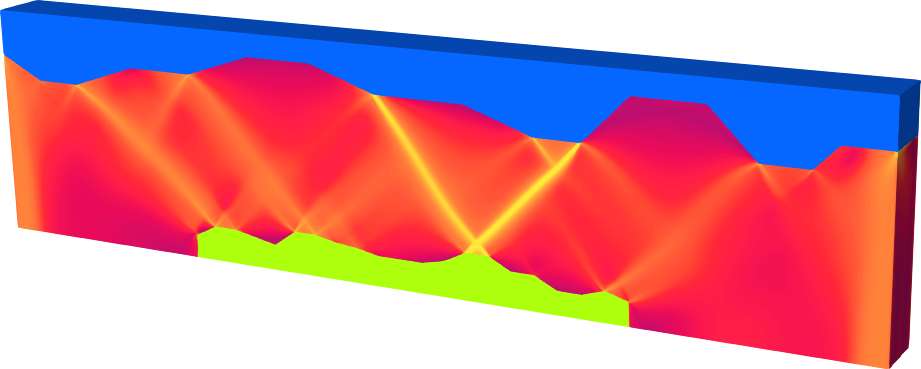
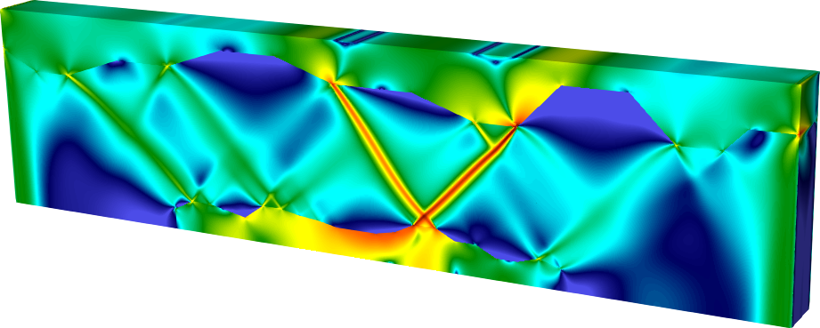
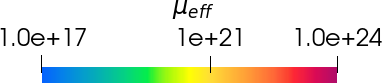
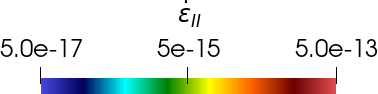
Figure 4: Effective viscosity (left) and the second invariant of the strain rate tensor (right) pertaining to the 3D compressional problem with composite rheology described in Section 5.3.

Figure 5: Number of iterations for solving the linearized Stokes systems ($y$-axis) in each Newton linearization ($x$-axis) for viscoplastic rheology problem. The average number of iterations for the linearized system are shown in parenthesis in the legend. The stress–velocity Newton solver is run until reaching $10^{8}$ nonlinear residual reduction. The discretization is based on $[\mathbb{Q}_{3}]^{3}\times\mathbb{P}_{2}^{\text{disc}}$ element with 25,122,399 unknowns. The multigrid hierarchy has 3 mesh levels. For solver settings (FGMRES, multigrid), see Table 2.

5.3.3 Linear and nonlinear convergence

Fig. 5 shows the convergence history for the nonlinear problem. First, we observe that using the AL preconditioner is necessary for the problem. For $\gamma=0$, i.e., the inverse viscosity-weighted pressure mass matrix as the Schur complement approximation in (4), the linear solver fails to solve the first stress–velocity Newton linearization within $300$ iterations. Second, the number of linear iterations required in each Newton step varies. For instance, the linearization arising in the $6$-th nonlinear iteration seems particularly difficult to solve. This happens as the linearized systems in different nonlinear iterations may have different characteristics and some may be more difficult to solve than others. On average, with large enough $\gamma$ ($\gamma>0.1$), the AL solver requires between 27 and 45 linear iterations. Lastly, we note that while the speed of convergence depends on the choice of $\gamma$, robust convergence is observed for a wide range of $\gamma$’s. In particular, values of $\gamma$ from $1$ to $1000$ result in an average of under 50 iterations per linear solve for a problem that could not be solved without the AL preconditioner.

5.3.4 Parallel scalability

Figure 6 shows the parallel scalability of the solver when applying to the nonlinear problem on hexahedral meshes with the $[\mathbb{Q}_{2}]^{3}\times\mathbb{P}_{1}^{\text{disc}}$ discretization. We note that as of writing, Firedrake only supports hexahedral meshes via extrusion of quadrilateral meshes, which has the consequence that only the two dimensional base mesh can be distributed in parallel. This limits the number of cores that can be used and makes the distribution over a large number of cores more challenging than in the case of tetrahedral meshes. For the slab domain under consideration, we are still able to scale to 1536 cores and 151 million unknowns, with a parallel efficiency of about 57% percent compared to a small run on 24 cores. We note that for the largest run, the maximum number of vertices and mesh elements on the finest level among MPI processes compared to the average number is $40\%$ and $18\%$ larger, respectively. A fourth run was not possible as then the number of cores would have exceeded the number of quadrilaterals in the base mesh.

Figure 6: Weak scalability results on NYU Greene for the first linear solve of the nonlinear Stokes problem with $\mathbf{P}_{2}$ with parameter robust multigrid solver for the (1,1)-block. The coarsest mesh is the same across the runs and the problem size is increased to maintain approximately 100k unknowns per core. With $l$ we indicate the number of refinement levels of the finest mesh compared to the coarse mesh. On the left we show the iterations numbers and the total times, and on the right the parallel efficiency of one multigrid cycle compared to the cycle on $24$ cores. The largest run has 151 million unknowns.

6 Conclusions

In this work we developed a scalable preconditioner for the Stokes equations with varying viscosity. The preconditioner combines an augmented Lagrangian term, a mass matrix based Schur complement approximation, and a robust multigrid scheme for the resulting nearly singular (1,1)-block. The two main contributions are eigenvalue estimate for the Schur complement approximation as well as a multigrid scheme for the (1,1)-block for the popular $[\mathbb{Q}_{k}]^{d}\times\mathbb{P}_{k-1}^{\text{disc}}$ discretization on quadrilateral/hexahedral meshes. Numerical experiments confirm robustness even for large viscosity contrasts, scalability to large problems in three dimensions, and show that the preconditioner can be combined with the stress-velocity Newton method of [57] to solve nonlinear Stokes flow with viscoplastic rheology. Finally, we remark that we expect that the approach here can be used for the development of preconditioners for the Navier-Stokes equations, in the same way that the multigrid scheme developed in [24] yields the Reynolds-robust preconditioner for the Navier–Stokes equations on simplicial meshes developed in [23].

References

- [1] M. S. Alnæs, A. Logg, K. B. Ølgaard, M. E. Rognes, and G. N. Wells, Unified form language: A domain-specific language for weak formulations of partial differential equations, ACM Transactions on Mathematical Software (TOMS), 40 (2014), pp. 1–37.
- [2] P. R. Amestoy, I. S. Duff, J.-Y. L’Excellent, and J. Koster, A fully asynchronous multifrontal solver using distributed dynamic scheduling, SIAM Journal on Matrix Analysis and Applications, 23 (2001), pp. 15–41.
- [3] P. R. Amestoy, A. Guermouche, J.-Y. L’Excellent, and S. Pralet, Hybrid scheduling for the parallel solution of linear systems, Parallel Computing, 32 (2006), pp. 136–156.
- [4] D. N. Arnold, R. S. Falk, and R. Winther, Preconditioning in and applications, Mathematics of Computation, 66 (1997), pp. 957–985, https://doi.org/10.1090/S0025-5718-97-00826-0.
- [5] D. N. Arnold, R. S. Falk, and R. Winther, Multigrid in and , Numerische Mathematik, 85 (2000), pp. 197–217, https://doi.org/10.1007/pl00005386.
- [6] S. Balay, W. D. Gropp, L. C. McInnes, and B. F. Smith, PETSc 2.0 users manual, Tech. Report ANL-95/11 - Revision 2.0.24, Argonne National Laboratory, 1999.
- [7] J. Bear, Dynamics of fluids in porous media, Courier Corporation, 2013.
- [8] M. Benzi and M. A. Olshanskii, An augmented Lagrangian-based approach to the Oseen problem, SIAM J. Sci. Comput., 28 (2006), pp. 2095–2113, https://doi.org/10.1137/050646421.
- [9] M. Benzi and M. A. Olshanskii, Field-of-values convergence analysis of augmented Lagrangian preconditioners for the linearized Navier–Stokes problem, SIAM Journal of Numerical Analysis, 49 (2011), pp. 770–788.
- [10] M. Benzi, M. A. Olshanskii, and Z. Wang, Modified augmented Lagrangian preconditioners for the incompressible Navier-Stokes equations, International Journal for Numerical Methods in Fluids, 66 (2011), pp. 486–508, https://doi.org/10.1002/fld.2267.
- [11] G. Bercea, A. T. T. McRae, D. A. Ham, L. Mitchell, F. Rathgeber, L. Nardi, F. Luporini, and P. H. J. Kelly, A structure-exploiting numbering algorithm for finite elements on extruded meshes, and its performance evaluation in firedrake, Geoscientific Model Development, 9 (2016), pp. 3803–3815, https://doi.org/10.5194/gmd-9-3803-2016.
- [12] S. Börm and S. L. Borne, -LU factorization in preconditioners for augmented Lagrangian and grad-div stabilized saddle point systems, International Journal for Numerical Methods in Fluids, 68 (2010), pp. 83–98, https://doi.org/10.1002/fld.2495.
- [13] D. Borzacchiello, E. Leriche, B. Blottière, and J. Guillet, Box-relaxation based multigrid solvers for the variable viscosity Stokes problem, Computers & Fluids, 156 (2017), pp. 515–525, https://doi.org/10.1016/j.compfluid.2017.08.027. Ninth International Conference on Computational Fluid Dynamics (ICCFD9).
- [14] D. Braess and R. Sarazin, An efficient smoother for the Stokes problem, Applied Numerical Mathematics, 23 (1997), pp. 3–19, https://doi.org/10.1016/S0168-9274(96)00059-1.
- [15] C. Burstedde, O. Ghattas, G. Stadler, T. Tu, and L. C. Wilcox, Parallel scalable adjoint-based adaptive solution for variable-viscosity Stokes flows, Computer Methods in Applied Mechanics and Engineering, 198 (2009), pp. 1691–1700, https://doi.org/10.1016/j.cma.2008.12.015.
- [16] B. Cockburn, G. Kanschat, and D. Schötzau, A note on discontinuous Galerkin divergence-free solutions of the Navier–Stokes equations, Journal of Scientific Computing, 31 (2006), pp. 61–73, https://doi.org/10.1007/s10915-006-9107-7.
- [17] M. Costabel and A. McIntosh, On Bogovskiĭ and regularized Poincaré integral operators for de Rham complexes on Lipschitz domains, Mathematische Zeitschrift, 265 (2010), pp. 297–320.
- [18] L. D. Dalcin, R. R. Paz, P. A. Kler, and A. Cosimo, Parallel distributed computing using Python, Advances in Water Resources, 34 (2011), pp. 1124–1139, https://doi.org/10.1016/j.advwatres.2011.04.013.
- [19] A. C. de Niet and F. W. Wubs, Two preconditioners for saddle point problems in fluid flows, International Journal for Numerical Methods in Fluids, 54 (2007), pp. 355–377, https://doi.org/10.1002/fld.1401.
- [20] D. Drzisga, L. John, U. Rüde, B. Wohlmuth, and W. Zulehner, On the analysis of block smoothers for saddle point problems, SIAM Journal on Matrix Analysis and Applications, 39 (2018), pp. 932–960, https://doi.org/10.1137/16M1106304.
- [21] H. C. Elman, D. J. Silvester, and A. J. Wathen, Finite elements and fast iterative solvers: with applications in incompressible fluid dynamics, Oxford University Press, 2014.
- [22] P. E. Farrell, M. G. Knepley, L. Mitchell, and F. Wechsung, PCPATCH: software for the topological construction of multigrid relaxation methods, Transactions on Mathematical Software, (2021), http://dro.dur.ac.uk/32553/.
- [23] P. E. Farrell, L. Mitchell, L. R. Scott, and F. Wechsung, A Reynolds-robust preconditioner for the Reynolds-robust Scott-Vogelius discretization of the stationary incompressible Navier-Stokes equations, arXiv preprint arXiv:2004.09398, (2020).
- [24] P. E. Farrell, L. Mitchell, L. R. Scott, and F. Wechsung, Robust multigrid methods for nearly incompressible elasticity using macro elements, arXiv preprint arXiv:2002.02051, (2020).
- [25] P. E. Farrell, L. Mitchell, and F. Wechsung, An augmented Lagrangian preconditioner for the 3D stationary incompressible Navier-Stokes equations at high Reynolds number, SIAM Journal on Scientific Computing, 41 (2019), pp. A3073–A3096.
- [26] M. Fortin and R. Glowinski, Augmented Lagrangian Methods: Applications to the Numerical Solution of Boundary-Value Problems, Elsevier, 2000.
- [27] M. Furuichi, D. A. May, and P. J. Tackley, Development of a Stokes flow solver robust to large viscosity jumps using a Schur complement approach with mixed precision arithmetic, Journal of Computational Physics, 230 (2011), pp. 8835–8851, https://doi.org/10.1016/j.jcp.2011.09.007.
- [28] T. Geenen, M. ur Rehman, S. P. MacLachlan, G. Segal, C. Vuik, A. P. van den Berg, and W. Spakman, Scalable robust solvers for unstructured FE geodynamic modeling applications: Solving the Stokes equation for models with large localized viscosity contrasts, Geochemistry Geophysics Geosystems, 10 (2009), p. Q09002, https://doi.org/10.1029/2009GC002526.
- [29] C. Geuzaine and J.-F. Remacle, Gmsh: A 3-d finite element mesh generator with built-in pre- and post-processing facilities, International Journal for Numerical Methods in Engineering, 79 (2009), pp. 1309–1331, https://doi.org/10.1002/nme.2579.
- [30] T. H. Gibson, L. Mitchell, D. A. Ham, and C. J. Cotter, Slate: extending firedrake’s domain-specific abstraction to hybridized solvers for geoscience and beyond, Geoscientific model development, 13 (2020), pp. 735–761.
- [31] P. P. Grinevich and M. A. Olshanskii, An iterative method for the Stokes-type problem with variable viscosity, SIAM Journal on Scientific Computing, 31 (2009), pp. 3959–3978, https://doi.org/10.1137/08744803.
- [32] S. Hamilton, M. Benzi, and E. Haber, New multigrid smoothers for the Oseen problem, Numerical Linear Algebra with Applications, (2010), https://doi.org/10.1002/nla.707.
- [33] X. He and M. Neytcheva, Preconditioning the incompressible Navier-Stokes equations with variable viscosity, Journal of Computational Mathematics, (2012), pp. 461–482.
- [34] X. He, M. Neytcheva, and S. S. Capizzano, On an augmented Lagrangian-based preconditioning of Oseen type problems, BIT Numerical Mathematics, 51 (2011), pp. 865–888, https://doi.org/10.1007/s10543-011-0334-4.
- [35] T. Heister and G. Rapin, Efficient augmented Lagrangian-type preconditioning for the Oseen problem using grad-div stabilization, International Journal for Numerical Methods in Fluids, 71 (2012), pp. 118–134, https://doi.org/10.1002/fld.3654.
- [36] B. Hendrickson and R. Leland, A multilevel algorithm for partitioning graphs, in Supercomputing ’95: Proceedings of the 1995 ACM/IEEE Conference on Supercomputing (CDROM), New York, 1995, ACM Press, p. 28, https://doi.org/10.1145/224170.224228.
- [37] V. Heuveline and F. Schieweck, On the inf-sup condition for higher order mixed FEM on meshes with hanging nodes, ESAIM: Mathematical Modelling and Numerical Analysis, 41 (2007), pp. 1–20.
- [38] M. Homolya and D. A. Ham, A parallel edge orientation algorithm for quadrilateral meshes, SIAM Journal on Scientific Computing, 38 (2016), pp. S48–S61, https://doi.org/10.1137/15M1021325.
- [39] M. Homolya, R. C. Kirby, and D. A. Ham, Exposing and exploiting structure: optimal code generation for high-order finite element methods, 2017, https://arxiv.org/abs/1711.02473.
- [40] M. Homolya, L. Mitchell, F. Luporini, and D. A. Ham, Tsfc: a structure-preserving form compiler, SIAM Journal on Scientific Computing, 40 (2018), pp. C401–C428.
- [41] Q. Hong, J. Kraus, J. Xu, and L. Zikatanov, A robust multigrid method for discontinuous Galerkin discretizations of Stokes and linear elasticity equations, Numerische Mathematik, 132 (2016), pp. 23–49, https://doi.org/10.1007/s00211-015-0712-y.
- [42] K. Hutter, Theoretical Glaciology, Mathematical Approaches to Geophysics, D. Reidel Publishing Company, 1983.
- [43] T. Isaac, G. Stadler, and O. Ghattas, Solution of nonlinear Stokes equations discretized by high-order finite elements on nonconforming and anisotropic meshes, with application to ice sheet dynamics, SIAM Journal on Scientific Computing, 37 (2015), pp. B804–B833, https://doi.org/10.1137/140974407.
- [44] G. Karypis and V. Kumar, A parallel algorithm for multilevel graph partitioning and sparse matrix ordering, Journal of Parallel and Distributed Computing, 48 (1998), pp. 71–95.
- [45] R. C. Kirby and L. Mitchell, Solver Composition Across the PDE/Linear Algebra Barrier, SIAM Journal on Scientific Computing, 40 (2018), pp. C76–C98, https://doi.org/10.1137/17M1133208.
- [46] F. Laakmann, P. E. Farrell, and L. Mitchell, An augmented Lagrangian preconditioner for the magnetohydrodynamics equations at high Reynolds and coupling numbers, arXiv preprint arXiv:2104.14855, (2021).
- [47] F. Luporini, D. A. Ham, and P. H. J. Kelly, An algorithm for the optimization of finite element integration loops, ACM Transactions on Mathematical Software, 44 (2017), pp. 3:1–3:26, https://doi.org/10.1145/3054944.
- [48] D. A. May, J. Brown, and L. L. Pourhiet, A scalable, matrix-free multigrid preconditioner for finite element discretizations of heterogeneous Stokes flow, Computer Methods in Applied Mechanics and Engineering, 290 (2015), pp. 496–523, https://doi.org/10.1016/j.cma.2015.03.014.
- [49] D. A. May and L. Moresi, Preconditioned iterative methods for Stokes flow problems arising in computational geodynamics, Physics of the Earth and Planetary Interiors, 171 (2008), pp. 33–47.
- [50] A. T. T. McRae, G.-T. Bercea, L. Mitchell, D. A. Ham, and C. J. Cotter, Automated generation and symbolic manipulation of tensor product finite elements, SIAM Journal on Scientific Computing, 38 (2016), pp. S25–S47, https://doi.org/10.1137/15M1021167.
- [51] J. Mewis and N. J. Wagner, Colloidal suspension rheology, Cambridge University Press, 2012.
- [52] L. Mitchell and E. H. Müller, High level implementation of geometric multigrid solvers for finite element problems: applications in atmospheric modelling, Journal of Computational Physics, 327 (2016), pp. 1–18, https://doi.org/10.1016/j.jcp.2016.09.037.
- [53] G. Ranalli, Rheology of the Earth, Springer, 1995.
- [54] R. Rannacher, Finite element methods for the incompressible Navier-Stokes equations, in Fundamental directions in mathematical fluid mechanics, Adv. Math. Fluid Mech., Birkhäuser, Basel, 2000, pp. 191–293.
- [55] F. Rathgeber, D. A. Ham, L. Mitchell, M. Lange, F. Luporini, A. T. T. McRae, G.-T. Bercea, G. R. Markall, and P. H. J. Kelly, Firedrake: automating the finite element method by composing abstractions, ACM Trans. Math. Softw., 43 (2016), pp. 24:1–24:27, https://doi.org/10.1145/2998441.
- [56] J. Rudi, A. C. I. Malossi, T. Isaac, G. Stadler, M. Gurnis, P. W. J. Staar, Y. Ineichen, C. Bekas, A. Curioni, and O. Ghattas, An extreme-scale implicit solver for complex PDEs: Highly heterogeneous flow in earth’s mantle, in SC15: Proceedings of the International Conference for High Performance Computing, Networking, Storage and Analysis, ACM, 2015, pp. 5:1–5:12, https://doi.org/10.1145/2807591.2807675.
- [57] J. Rudi, Y.-h. Shih, and G. Stadler, Advanced Newton methods for geodynamical models of stokes flow with viscoplastic rheologies, Geochemistry, Geophysics, Geosystems, 21 (2020), p. e2020GC009059, https://doi.org/10.1029/2020GC009059.
- [58] J. Rudi, G. Stadler, and O. Ghattas, Weighted BFBT preconditioner for Stokes flow problems with highly heterogeneous viscosity, SIAM Journal on Scientific Computing, 39 (2017), pp. S272–S297, https://doi.org/10.1137/16M108450X.
- [59] J. Schoeberl, Robust Multigrid Methods for Parameter Dependent Problems, PhD thesis, 1999.
- [60] L. R. Scott and S. Zhang, Finite element interpolation of nonsmooth functions satisfying boundary conditions, Mathematics of Computation, 54 (1990), pp. 483–493, http://www.jstor.org/stable/2008497.
- [61] M. Spiegelman, D. A. May, and C. R. Wilson, On the solvability of incompressible Stokes with viscoplastic rheologies in geodynamics, Geochemistry, Geophysics, Geosystems, 17 (2016), pp. 2213–2238.
- [62] M. ur Rehman, C. Vuik, and G. Segal, A comparison of preconditioners for incompressible Navier-Stokes solvers, International Journal for Numerical Methods in Fluids, 57 (2008), pp. 1731–1751, https://doi.org/10.1002/fld.1684.
- [63] S. P. Vanka, Block-implicit multigrid solution of Navier-Stokes equations in primitive variables, Journal of Computational Physics, 65 (1986), pp. 138–158.
- [64] M. Wang and L. Chen, Multigrid methods for the Stokes equations using distributive Gauss—Seidel relaxations based on the least squares commutator, J. Sci. Comput., 56 (2013), p. 409–431, https://doi.org/10.1007/s10915-013-9684-1.
- [65] F. Wechsung, Shape Optimisation and Robust Solvers for Incompressible Flow, PhD thesis, University of Oxford, 2019.
- [66] J. Xia, P. E. Farrell, and F. Wechsung, Augmented Lagrangian preconditioners for the Oseen-Frank model of nematic and cholesteric liquid crystals, BIT Numerical Mathematics, 61 (2021), pp. 607–644, https://doi.org/10.1007/s10543-020-00838-9.