Surface Bogoliubov-Dirac cones and helical Majorana hinge modes
in superconducting Dirac semimetals

Abstract

In the presence of certain symmetries, three-dimensional Dirac semimetals can harbor not only surface Fermi arcs, but also surface Dirac cones. Motivated by the experimental observation of rotation-symmetry-protected Dirac semimetal states in iron-based superconductors, we investigate the potential intrinsic topological phases in a $C_{4z}$-rotational invariant superconducting Dirac semimetal with $s_{\pm}$-wave pairing. When the normal state harbors only surface Fermi arcs on the side surfaces, we find that an interesting gapped superconducting state with a quartet of Bogoliubov-Dirac cones on each side surface can be realized, even though the first-order topology of its bulk is trivial. When the normal state simultaneously harbors surface Fermi arcs and surface Dirac cones, we find that a second-order time-reversal invariant topological superconductor with helical Majorana hinge states can be realized. The criteria for these two distinct topological phases have a simple geometric interpretation in terms of three characteristic surfaces in momentum space. By reducing the bulk material to a thin film normal to the axis of rotation symmetry, we further find that a two-dimensional first-order time-reversal invariant topological superconductor can be realized if the inversion symmetry is broken by applying a gate voltage. Our work reveals that diverse topological superconducting phases and types of Majorana modes can be realized in superconducting Dirac semimetals.

I Introduction

Topological superconductors (TSCs) are a class of novel phases with exotic gapless boundary excitations known as Majorana modes Read and Green (2000); Kitaev (2001). Over the past decade, the pursuit of TSCs and Majorana modes in real materials has attracted a great amount of enthusiasm Alicea (2012); Leijnse and Flensberg (2012); Beenakker (2013); Stanescu and Tewari (2013); Elliott and Franz (2015); Sato and Fujimoto (2016); Aguado (2017); Haim and Oreg (2019); Jäck et al. (2021), owing to their exotic properties and potential applications in topological quantum computation Ivanov (2001); Alicea et al. (2011); Nayak et al. (2008); Sarma et al. (2015). Very recently, an important form of progress on the theoretical side is the birth of the concept named higher-order TSCs Benalcazar et al. (2017a); Schindler et al. (2018); Benalcazar et al. (2017b); Song et al. (2017); Langbehn et al. (2017); Khalaf (2018); Geier et al. (2018); Zhu (2018); Yan et al. (2018); Wang et al. (2018a, b); Yan (2019a), which not only enriches the physics of TSCs, but also provides new perspectives for the realization and applications of Majorana modes Shapourian et al. (2018); Hsu et al. (2018); Liu et al. (2018a); Wu et al. (2019); Zhang et al. (2019a, b); Volpez et al. (2019); Zhu (2019); Peng and Xu (2019); Ghorashi et al. (2019); Yan (2019b); Bultinck et al. (2019); Franca et al. (2019); Pan et al. (2019); Kheirkhah et al. (2020a, b); Wu et al. (2020a); Hsu et al. (2020); Wu et al. (2020b); Laubscher et al. (2020); Tiwari et al. (2020); Ahn and Yang (2020); Roy (2020); Li and Yan (2021); Niu et al. (2021); Wu et al. (2021a); Fu et al. (2021); Luo et al. (2021); Jahin et al. (2021); Qin et al. (2021); Tan et al. (2021); You et al. (2019); Zhang et al. (2020a, b); Pahomi et al. (2020); Bomantara and Gong (2020); Lapa et al. (2021); Ikegaya et al. (2021); Roy and Juricic (2021). The most prominent difference between conventional TSCs and their higher-order counterparts lies in the bulk-boundary correspondence, or more precisely, the codimension $d_{c}$ of the gapless Majorana modes at the boundary. To be specific, a conventional TSC has $d_{c}=1$, while an $n$th-order TSC has $d_{c}=n\geq 2$. Conventional TSCs are thus also dubbed as first-order TSCs. One direct significance of this extension is that a lot of systems previously thought to be trivial in the framework of first-order topology are recognized to be nontrivial in the framework of higher-order topology.

Because of the scarcity of odd-parity superconductors in nature, the realization of both first-order and second-order TSCs heavily relies on materials with strong spin-orbit coupling or topological band structure Fu and Kane (2008); Lutchyn et al. (2011); Oreg et al. (2010); Sau et al. (2010); Alicea (2010); Yan et al. (2018); Wang et al. (2018a); Zhu (2019); Kheirkhah et al. (2020b). By far, most experiments in this field have focused on the realization of first-order TSCs in various kinds of heterostructures which simultaneously consist of three ingredients, namely, spin-orbit coupling, magnetism or external magnetic fields, and $s$-wave superconductivity Mourik et al. (2012); Rokhinson et al. (2012); Das et al. (2012); Deng et al. (2012); Finck et al. (2013); Nadj-Perge et al. (2014); Sun et al. (2016); Deng et al. (2016); Fornieri et al. (2019); Ren et al. (2019). Despite steady progress in experiments, the complexity of such heterostructures and the concomitant strong inhomogeneity make a definitive confirmation of the expected Majorana modes remain elusive Zhang et al. (2019c); Frolov et al. (2020); Yu et al. (2021). Since these common shortcomings of heterostructures shadow the pursuit of Majorana modes and are quite challenging to overcome in the short term, intrinsic TSCs become highly desired to make further breakthroughs. Remarkably, the band structures of a series of iron-based superconductors have recently been observed to host both topological insulator states and rotation-symmetry-protected Dirac semimetal (DSM) states near the Fermi level Zhang et al. (2018, 2019d). Since the coexistence of topological insulator states and superconductivity provides a realization of the Fu-Kane proposal Fu and Kane (2008) in a single material, the potential existence of Majorana zero modes in the vortices of these iron-based superconductors has attracted great attention Wang et al. (2018c); Liu et al. (2018b); Machida et al. (2019); Kong et al. (2019); Zhu et al. (2020); Jiang et al. (2019); Qin et al. (2019a); Chiu et al. (2020); Ghazaryan et al. (2020); Wu et al. (2021b); Kheirkhah et al. (2021). In addition, it turns out that the combination of topological insulator states and unconventional $s_{\pm}$-wave pairing also makes these iron-based superconductors promising for the realization of intrinsic higher-order TSCs Zhang et al. (2019a); Kheirkhah et al. (2021). Compared with the topological insulator states, we notice that the DSM states in these iron-based superconductors have been explored much less Qin et al. (2019b); König and Coleman (2019); Yan et al. (2020); Kawakami and Sato (2019).

Motivated by the above observation, we explore the potential intrinsic topological phases in superconducting DSMs with $s_{\pm}$-wave pairing. However, instead of considering a realistic but complicated Hamiltonian to accurately produce the band structure of one specific iron-based superconductor, we will take a minimal-Hamiltonian approach for generality, so that the results can be applied to all DSMs with the same symmetry and topological properties. To be relevant to iron-based superconductors, in this paper we focus on DSMs protected by $C_{4z}$-rotation symmetry Yang and Nagaosa (2014). For DSMs, while the low-energy physics in the bulk can be universally described by linear continuum Dirac Hamiltonians, the gapless states on the boundary, however, are sensitive to the details of the full lattice Hamiltonian. An important fact is that both surface Fermi arcs and surface Dirac cones are symmetry allowed in DSMs Kobayashi and Sato (2015); Kargarian et al. (2016); Yan et al. (2020); Wieder et al. (2020). As a consequence, we find that depending on whether surface Fermi arcs and surface Dirac cones coexist or not, a second-order time-reversal invariant TSC with helical Majorana hinge modes or an interesting gapped phase with a quartet of Bogoliubov-Dirac cones on each side surface can be realized in the superconducting DSM, respectively. By reducing the dimension of the second-order time-reversal invariant TSC from three dimensions to a thin film, we find that a first-order time-reversal invariant TSC can be realized if the inversion symmetry is broken by applying an external gate voltage. These findings suggest that the superconducting DSM on its own can realize a diversity of intrinsic TSCs.

The paper is organized as follows. In Sec. II, the topological properties of the normal state are investigated. In Sec. III, we show that two superconducting phases with distinct topological boundary states can be realized in superconducting DSMs. In Sec. IV, we show that thin films of a superconducting DSM can realize first-order time-reversal invariant TSCs. Finally, we conclude with a discussion in Sec. V. Some calculation details are relegated to Appendices A and B.

II Topological properties of the normal state

We start with the DSM Hamiltonian which, in the basis $\psi^{{\dagger}}_{\bm{k}}=(c_{a,\uparrow,\bm{k}}^{{\dagger}},c_{b,\uparrow,\bm{k}}^{{\dagger}},c_{a,\downarrow,\bm{k}}^{{\dagger}},c_{b,\downarrow,\bm{k}}^{{\dagger}})$, reads Yang and Nagaosa (2014)

$$H_{\rm DSM}(\bm{k}) = [m-t(\cos k_{x}+\cos k_{y})-t_{z}\cos k_{z}]\sigma_{z}$$ (1)

$$+\lambda\sin k_{x}s_{z}\sigma_{x}+\eta\sin k_{z}(\cos k_{x}-\cos k_{y})s_{x}\sigma_{x}$$

$$-\lambda\sin k_{y}\sigma_{y}+2\eta\sin k_{x}\sin k_{y}\sin k_{z}s_{y}\sigma_{x},$$

where the Pauli matrices $\sigma_{i}$ and $s_{i}$ act on the orbital ($a,b$) and spin ($\uparrow,\downarrow$) degrees of freedom, respectively. For notational simplicity, the lattice constants are set to unity throughout this paper, and identity matrices are always made implicit. The Hamiltonian simultaneously has time-reversal symmetry ($\mathcal{T}=is_{y}\mathcal{K}$, with $\mathcal{K}$ denoting complex conjugation), inversion symmetry ($I=\sigma_{z}$), and $C_{4z}$-rotation symmetry ($C_{4z}=\text{diag}\{e^{-3i\pi/4},e^{-i\pi/4},e^{3i\pi/4},e^{i\pi/4}\}$), which thus allows the presence of robust Dirac points on the rotation symmetry axis. It is easy to find that Dirac points will appear as long as the band inversion surface (BIS), which is defined as the zero-value contour of $m-t(\cos k_{x}+\cos k_{y})-t_{z}\cos k_{z}$ in momentum space, encloses one time-reversal invariant momentum.

Usually, as the two symmetry-allowed $\eta$ terms in Eq. (1) only contribute cubic-order terms in momentum to the continuum Dirac Hamiltonian, they are neglected. While it is true that their higher-order contributions to the bulk can be safely neglected when focusing on the low-energy physics near the Dirac points, it has been demonstrated that their impact on the surface states, however, is significant Kargarian et al. (2016); Yan et al. (2020); Le et al. (2018). Without the two $\eta$ terms ($\eta=0$), the DSM is found to harbor only Fermi arcs on the side surfaces. Remarkably, once the two $\eta$ terms are present ($\eta\neq 0$), the DSM harbors not only Fermi arcs on the side surfaces, but also a single Dirac cone on each of the surfaces of a cubic-geometry sample, resembling the surface Dirac cones in strong topological insulators. To have an intuitive picture of the qualitative difference between $\eta=0$ and $\eta\neq 0$, we take $\{m,t,t_{z},\lambda\}=\{3,2,2,1\}$ so that the Dirac points are localized at $\bm{k}_{D;\pm}=\pm(0,0,2\pi/3)$ and then diagonalize the Hamiltonian in a cubic geometry with open boundary conditions in one direction and periodic boundary conditions in the other two orthogonal directions. The corresponding energy spectra shown in Fig. 1 clearly manifest the qualitative difference in surface states between $\eta=0$ and $\eta\neq 0$. As we will show below, this remarkable difference will lead to distinct topological superconducting states.

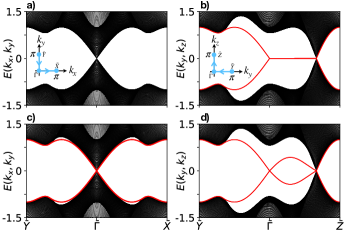
Figure 1: (Color online) Surface band structure for the normal state. Common parameters are $m=3$, $t=t_{z}=2$, $\lambda=1$. $\eta=0$ in (a) and (b), and $\eta=0.5$ in (c) and (d). Surface Dirac cones are absent in (a) and (b) and present in (c) and (d) at the center of the surface Brillouin zone. In each panel, the side with open boundary conditions is 200 lattice sites long.

III Topological properties of superconducting Dirac semimetals

Let us now focus on the superconducting state. Within the mean-field framework, the Hamiltonian becomes $H=\frac{1}{2}\sum_{\bm{k}}\Psi_{\bm{k}}^{{\dagger}}H_{\rm BdG}(\bm{k})\Psi_{\bm{k}}$, with $\Psi_{\bm{k}}^{{\dagger}}=(\psi_{\bm{k}}^{{\dagger}},\psi_{-\bm{k}})$ and the corresponding Bogoliubov-de Gennes (BdG) Hamiltonian takes the form

$$H_{\rm BdG}(\bm{k}) = \left(\begin{array}[]{cc}H_{\rm DSM}(\bm{k})-\mu&-is_{y}\Delta(\bm{k})\\ is_{y}\Delta(\bm{k})&\mu-H_{\rm DSM}^{*}(-\bm{k})\\ \end{array}\right),$$ (4)

where $\Delta(\bm{k})=\Delta_{0}-\Delta_{s}(\cos k_{x}+\cos k_{y})$ characterizes the $s_{\pm}$-wave pairing. Since the BdG Hamiltonian simultaneously has time-reversal symmetry and particle-hole symmetry, it belongs to the DIII class in the ten-fold way classification Schnyder et al. (2008); Kitaev (2009). Accordingly, its first-order topology is characterized by a winding number $N_{w}$ and follows a $\mathbb{Z}$ classification in three dimensions. When $N_{w}$ is a nonzero integer in a gapped superconductor, the bulk-boundary correspondence tells us that there are $N_{w}$ robust Majorana cones on an arbitrary surface Roy (2008); Qi et al. (2009); Volovik (2009), irrespective of its orientation. A simple formula for $N_{w}$ valid in the weak-pairing limit is Qi et al. (2010)

$$N_{w}=\frac{1}{2}\sum_{n}\text{sgn}(\Delta_{i})C_{1i},$$ (5)

where $C_{1i}$ denotes the first Chern number and $\text{sgn}(\Delta_{i})$ denotes the sign of pairing on the $i$th Fermi surface. Since the simultaneous preservation of time-reversal symmetry and inversion symmetry forces $C_{1i}$ to vanish, $N_{w}$ thus identically vanishes, indicating that the first-order topology is always trivial for this Hamiltonian. Despite the absence of nontrivial first-order topology, the superconducting DSM, nevertheless, can be nontrivial in the higher-order topology and host interesting Majorana modes on the boundary.

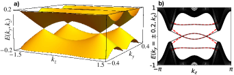
Figure 2: (Color online) Chosen parameters are $m=3$, $t=t_{z}=2$, $\lambda=1$, $\eta=0$, $\mu=0.2$, and $\Delta_{0}=\Delta_{s}=0.2$. Accordingly, $R_{\rm FS}=0.2$, $R_{\rm PNS}=\sqrt{2}$, and $R_{\rm BIS}=\sqrt{3}$. (a) The two middle bands of the surface Hamiltonian in Eq. (6) touch at $(k_{y},k_{z})=(\pm 0.2,\pm 1)$, forming four gapless Bogoliubov-Dirac cones. (b) Energy spectrum along $k_{y}=\pm 0.2$. The surface bands obtained from the low-energy analytical approach (midgap red dashed lines) agree excellently with those obtained by directly diagonalizing the full lattice Hamiltonian (midgap black solid lines, doubly degenerate) under open boundary conditions in the $x$ direction, confirming the existence of four gapless Bogoliubov-Dirac cones on each of the two $x$-normal surfaces.

The bulk spectrum of the superconducting DSM is gapped as long as the pairing node surface (PNS), which is the zero-value contour of $\Delta(\bm{k})$ in momentum space, does not cross the Fermi surface. On the boundary, the presence of superconductivity is also expected to gap out the topological surface states. An interesting question is whether it is possible that while the bulk states are fully gapped, the topological surface states are not fully gapped, so that there emerge certain types of gapless Bogoliubov quasiparticles on the boundary. We find that the answer is affirmative. To show this, the most intuitive approach is to derive the low-energy Hamiltonian for the surface states. Without loss of generality, we focus on the left $x$-normal surface and assume that the parameters $m$, $t$, and $t_{z}$ are chosen such that the BIS encloses the time-reversal invariant momentum $\bm{\Gamma}=(0,0,0)$. Following a standard approach, we expand the lattice Hamiltonian around $\bm{\Gamma}$ to obtain the continuum bulk Hamiltonian and then find that the corresponding low-energy surface Hamiltonian takes the form (see Appendix A)

$$H_{s}(k_{y},k_{z}) \approx \lambda k_{y}s_{z}+v_{z}(k_{y},k_{z})k_{z}\tau_{z}s_{y}-\mu\tau_{z}$$ (6)

$$+\frac{\Delta_{s}}{2}\left(R_{\rm BIS}^{2}-R_{\rm PNS}^{2}-\frac{t_{z}}{t}k_{z}^{2}\right)\tau_{y}s_{y},$$

where $v_{z}(k_{y},k_{z})=-\eta(\tilde{m}+tk_{y}^{2}+t_{z}k_{z}^{2}/2)/t$ with $\tilde{m}=m-2t-t_{z}$, $R_{\rm BIS}=\sqrt{-2\tilde{m}/t}$, and $R_{\rm PNS}=\sqrt{-2\tilde{\Delta}/\Delta_{s}}$ with $\tilde{\Delta}=\Delta_{0}-2\Delta_{s}$. Here, we have already assumed $\{t,t_{z},\lambda,\Delta_{s}\}>0$ and $\{\tilde{m},\tilde{\Delta}\}<0$. According to the continuum bulk Hamiltonian, $R_{\rm BIS}$ and $R_{\rm PNS}$ correspond to the radii of BIS and PNS in the $k_{z}=0$ plane, respectively. It is worth noting that the surface states only exist in the regime satisfying $tk_{y}^{2}+t_{z}k_{z}^{2}<-2\tilde{m}$, which is just the projection of BIS in the $k_{x}$ direction.

Let us first consider the $\eta=0$ case, where $v_{z}=0$ in this limit. Accordingly, the normal state has only Fermi arcs which are two straight lines at $k_{y}=\pm R_{\rm FS}$, where $R_{\rm FS}=|\mu/\lambda|$ corresponds to the maximum radius of the Fermi surface in the $k_{x}$-$k_{y}$ plane. The geometric meaning of this expression is that the Fermi arcs tangentially connect with the projection of the Fermi surface in the surface Brillouin zone Haldane (2014). Taking into account superconductivity, we find from Eq. (6) that the surface energy bands harbor four cones with linear dispersion at $(k_{y},k_{z})=(\pm R_{\rm FS},\pm\sqrt{t(R_{\rm BIS}^{2}-R_{\rm PNS}^{2})/t_{z}})$ if $R_{\rm BIS}>R_{\rm PNS}$. As the Bogoliubov quasiparticle operators associated with these surface cones do not satisfy the self-conjugate property ($\gamma_{\bm{k}}^{{\dagger}}=\gamma_{-\bm{k}}$ with $\gamma_{\bm{k}}^{{\dagger}}$ denoting the quasiparticle creation operator at momentum $\bm{k}$), we dub them Bogoliubov-Dirac cones to distinguish them from charge-neutral Majorana cones. Recalling that the precondition for this result is $tk_{y}^{2}+t_{z}k_{z}^{2}<-2\tilde{m}$, we find that the criterion for the existence of surface Bogoliubov-Dirac cones needs to be modified as $R_{\rm FS}<R_{\rm PNS}<R_{\rm BIS}$. This criterion corresponds to a simple geometric picture, namely, the PNS simultaneously encloses the bulk Fermi surface and intersects the BIS. In Fig. 2, we provide numerical results to show the existence of four gapless Bogoliubov-Dirac cones on each of the side surfaces (note that the system has $C_{4z}$-rotation symmetry) when the above-mentioned criterion is fulfilled. Before proceeding to $\eta\neq 0$, it is worth pointing out that every gapless Bogoliubov-Dirac cone has a topological protection due to the existence of chiral symmetry (the product of particle-hole symmetry and time-reversal symmetry) which will assign a topological winding number to characterize the band touching points of the surface energy spectrum Ryu et al. (2010) (see Appendix A). Accordingly, one gapless Bogoliubov-Dirac cone can be gapped only when it meets another gapless Bogoliubov-Dirac cone characterized by an opposite winding number.

Now we turn to the $\eta\neq 0$ case for which surface Fermi arcs and Dirac cones coexist in the normal state. According to Eq. (6), we find that if the energy spectrum harbors gapless Bogoliubov-Dirac cones at $\eta=0$, these persist for nonzero $\eta$ as long as $|\eta|<\eta_{c}=\frac{2|\mu|}{R_{\rm PNS}^{2}}\sqrt{\frac{t_{z}}{t(R_{\rm BIS}^{2}-R_{\rm PNS}^{2})}}$. However, with the increase in $\eta$, the surface Bogoliubov-Dirac cones approach one another and become gapped pairwise when $|\eta|>\eta_{c}$, resulting in a fully gapped surface energy spectrum (see Appendix A). Remarkably, after gapping out the surface Bogoliubov-Dirac cones, we find that the superconductor becomes a second-order time-reversal invariant TSC with helical Majorana hinge modes. To have an intuitive understanding of this transition, here we take the special case with $\mu=0$ for an analytical illustration. For this special case, $\eta_{c}=0$, suggesting that arbitrarily weak $\eta$ terms will gap out the surface Bogoliubov-Dirac cones. Focusing on the small momentum region, the surface Hamiltonian in Eq. (6) can be simplified by neglecting the cubic-order momentum terms as

$$H_{s}(k_{y},k_{z}) =-\frac{\tilde{m}\eta}{t}k_{z}\tau_{z}s_{y}+\frac{\Delta_{s}}{2}(R_{\rm BIS}^{2}-R_{\rm PNS}^{2}-\frac{t_{z}}{t}k_{z}^{2})\tau_{y}s_{y}$$

$$\quad+\lambda k_{y}s_{z}.$$ (7)

When $\eta\neq 0$ and $R_{\rm BIS}>R_{\rm PNS}$, the first line realizes a one-dimensional (1D) time-reversal invariant TSC in the $k_{z}$ direction Shen (2013). Considering a half-infinity surface occupying the region $0\leq z<+\infty$, doing the replacement $k_{z}\rightarrow-i\partial_{z}$ and solving the eigenvalue equation $H_{s}\phi_{\alpha}(z)=E_{\alpha}\phi_{\alpha}(z)$ under boundary conditions $\phi_{\alpha}(0)=\phi_{\alpha}(+\infty)=0$, one will find the existence of two branches of charge-neutral midgap states with opposite spin polarizations on the boundary of the surface, with their dispersions given by $E_{\alpha=1,2}=\pm\lambda k_{y}$ (see Appendix A), indicating the appearance of helical Majorana modes on the hinges. In Fig. 3, we further provide numerical results for $\mu\neq 0$ to support the realization of a second-order time-reversal invariant TSC with helical Majorana hinge modes when the criterion established above is fulfilled.

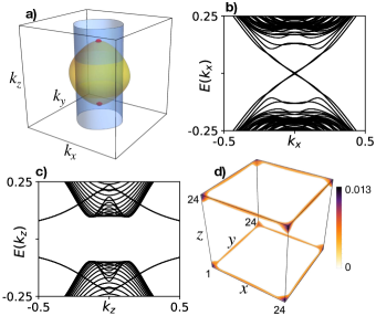
Figure 3: (Color online) Chosen parameters are $m=3$, $t=t_{z}=2$, $\lambda=\eta=1$, $\mu=0.2$, and $\Delta_{0}=\Delta_{s}=0.2$. (a) The PNS (blue), the BIS (yellow), and the two Fermi surfaces (red). (b) Helical Majorana hinge modes along the $x$ direction. Both $y$ and $z$ directions have open boundary conditions with $N_{y}=N_{z}=60$ lattice sites. (c) No gapless hinge modes along the $z$ direction. Both $x$ and $y$ directions have open boundary conditions with $N_{x}=N_{y}=50$. (d) The probability density distribution of the four eigenstates whose energies are in the middle of the BdG energy spectrum, confirming the localization of the helical Majorana modes on the hinges. All three directions have open boundary conditions with $N_{x}=N_{y}=N_{z}=24$.

IV First-order time-reversal invariant topological superconductivity in thin-film superconducting Dirac semimetals

For $s_{\pm}$-wave pairing, we have shown that the first-order topology is always trivial when time-reversal symmetry and inversion symmetry are preserved simultaneously. In the following, we consider reducing the bulk superconducting DSM to a thin film along the $z$ direction so that inversion symmetry can be easily broken by applying a gate voltage to the top and bottom layers Zhang and Das Sarma (2021). Remarkably, we find that when $\eta\neq 0$, a first-order time-reversal invariant TSC can be achieved (a discussion of the $\eta=0$ case is provided in Appendix B). It is worth noting that although the thin-film superconducting DSM still belongs to class DIII, the classification of the gapped phases is changed from $\mathbb{Z}$ to $\mathbb{Z}_{2}$ due to the dimensional reduction, with the $\mathbb{Z}_{2}$ invariant given in the weak-pairing limit by Qi et al. (2010)

$$N_{\rm 2D}=\prod_{i}[\text{sgn}(\Delta_{i})]^{m_{i}}.$$ (8)

Here, $m_{i}$ counts the number of time-reversal invariant momenta enclosed by the $i$th Fermi surface, and $N_{\rm 2D}=-1$ indicates the realization of a first-order time-reversal invariant TSC with helical Majorana edge modes Qi et al. (2009); Nakosai et al. (2012); Zhang et al. (2013); Wang et al. (2014); Parhizgar and Black-Schaffer (2017); Casas et al. (2019); Zhang and Das Sarma (2021).

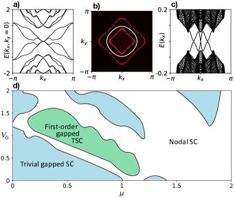
Figure 4: (Color online) Chosen parameters are $m=3$, $t=t_{z}=2$, $\lambda=\eta=1$, and $N_{z}=5$. a) The normal-state energy spectrum along the $k_{y}=0$ line at $V_{0}=1$. b) The configurations of pairing line node (white) and Fermi surfaces (red) in the two-dimensional Brillouin zone for $\Delta_{0}=\Delta_{s}=0.2$, $\mu=0.7$ and $V_{0}=1$. c) With the same set of parameters as in b), the energy spectrum shows the existence of $\mathbb{Z}_{2}$ nontrivial helical Majorana modes in the gap when open boundary conditions are taken in both $y$ and $z$ directions with $N_{y}=100$. The two tiny gaps at finite momentum are intrinsic and correspond to avoided crossings. d) The phase diagram includes three topologically distinct phases.

To be specific, here we consider the number of layers to be $N_{z}=5$ and add a potential profile of the form $V(z)\psi_{k_{x},k_{y},z}^{{\dagger}}\psi_{k_{x},k_{y},z}$ to the BdG Hamiltonian, where $V(z)=V_{0}(2z-N_{z}-1)/(N_{z}-1)$ with $z=1,2,...,N_{z}$, i.e. the gate voltage varies linearly across the sample, so the voltage difference between top and bottom layers is $2V_{0}$. With the same set of parameters as in the bulk case, the corresponding normal-state energy spectra for the thin film are shown in Fig. 4(a). One finds that, in this case, the normal state is a two-dimensional semimetal with spin-split dispersion (away from time-reversal invariant momenta). Assuming the location of PNS to be fixed, we find that tuning the chemical potential can make the PNS fall between two disconnected Fermi surfaces, as shown in Fig. 4(b). In accordance with Eq. (8), it is readily found that $N_{\rm 2D}$ takes the nontrivial value $-1$ for the configuration in Fig. 4(b). By numerically calculating the energy spectra in a cylinder geometry, the existence of robust midgap helical Majorana edge modes confirms the realization of a first-order time-reversal invariant TSC, as shown in Fig. 4(c). Moreover, the phase diagram in Fig. 4(d) shows that, for a broad regime of $\mu$, the thin-film superconducting DSM can be made topologically nontrivial by tuning the gate voltage.

V Discussion and conclusion

We have uncovered topological criteria for the realization of surface Bogoliubov-Dirac cones and helical Majorana hinge modes in three-dimensional superconducting DSMs with $s_{\pm}$-wave pairing. Remarkably, the topological criteria admit a simple geometric interpretation in terms of the relative configurations of BIS, PNS, and Fermi surface. We have also shown that first-order time-reversal invariant TSCs can be realized in thin-film superconducting DSMs by applying a gate voltage to break inversion symmetry. Our work suggests that intrinsic superconductors simultaneously hosting a gapless Dirac band structure and unconventional superconductivity can realize a diversity of intrinsic time-reversal invariant TSCs and Majorana modes. Our predictions can be tested in iron-based superconductors such as LiFe_1-xCo_xAs Zhang et al. (2019d) by adjusting the doping level so as to position the Fermi energy near the bulk Dirac points. Experimentally, the surface Bogoliubov-Dirac cones can be detected by angle-resolved photoemission spectroscopy Zhang et al. (2018, 2019d), and the helical Majorana modes can be measured by scanning tunneling microscopy Kezilebieke et al. (2020) as well as contact methods Gray et al. (2019).

Appendix A Derivation of the low-energy Hamiltonian for the surface states

We start with the full Bogoliubov-de Gennes (BdG) lattice Hamiltonian, which reads

$$H_{\rm BdG}(\bm{k}) =[m-t(\cos k_{x}+\cos k_{y})-t_{z}\cos k_{z}]\tau_{z}\sigma_{z}$$

$$\quad+\lambda(\sin k_{x}s_{z}\sigma_{x}-\sin k_{y}\tau_{z}\sigma_{y})-\mu\tau_{z}$$

$$\quad+\eta\sin k_{z}(\cos k_{x}-\cos k_{y})s_{x}\sigma_{x}$$

$$\quad+2\eta\sin k_{x}\sin k_{y}\sin k_{z}\tau_{z}s_{y}\sigma_{x}$$

$$\quad+[\Delta_{0}-\Delta_{s}(\cos k_{x}+\cos k_{y})]\tau_{y}s_{y},$$ (9)

where the Pauli matrices $\sigma_{i}$, $s_{i}$, and $\tau_{i}$ act on the orbital, spin, and particle-hole degrees of freedom, respectively. Similar to the main text, the lattice constants are set to unity and the identity matrices are made implicit for brevity. To derive the low-energy Hamiltonian for the surface states, without loss of generality, we consider that the band inversion surface (BIS) only encloses one time-reversal invariant momentum, $\bm{\Gamma}=(0,0,0)$. Accordingly, we expand the lattice Hamiltonian around $\bm{\Gamma}$ to obtain the corresponding continuum bulk Hamiltonian, which reads

$$H_{c}(\bm{k}) =\left[\tilde{m}+\frac{t}{2}(k_{x}^{2}+k_{y}^{2})+\frac{t_{z}}{2}k_{z}^{2}\right]\tau_{z}\sigma_{z}$$

$$\quad+\lambda(k_{x}s_{z}\sigma_{x}-k_{y}\tau_{z}\sigma_{y})-\mu\tau_{z}$$

$$\quad-\frac{\eta}{2}k_{z}(k_{x}^{2}-k_{y}^{2})s_{x}\sigma_{x}+2\eta k_{z}k_{x}k_{y}\tau_{z}s_{y}\sigma_{x}$$

$$\quad+\left[\tilde{\Delta}+\frac{\Delta_{s}}{2}(k_{x}^{2}+k_{y}^{2})\right]\tau_{y}s_{y},$$ (10)

where $\tilde{m}=m-2t-t_{z}$ and $\tilde{\Delta}=\Delta_{0}-2\Delta_{s}$. Before proceeding, it is worth noting that while the low-energy bulk physics is dominated by the gapless bulk Dirac cones, one cannot use the low-energy bulk Hamiltonian expanded around the Dirac points to extract the low-energy boundary Hamiltonian describing the surface states; instead, one needs to use the low-energy bulk Hamiltonian expanded around the band inversion momentum (above we have assumed it to be $\bm{\Gamma}$). The surface states originate from the band inversion, so one should expand around the band inversion momentum to take into account the full band inversion region. On the other hand, the locations of Dirac points correspond to the boundary of the band inversion surface along the rotation-symmetric axis, so in fact one cannot obtain the surface-state information through the low-energy Hamiltonian expanded around the Dirac points. In addition, it is also worth noting that we have only kept the leading term in momentum for each term in the continuum bulk Hamiltonian for simplicity. Such an approximation allows a simple analytic derivation of the low-energy boundary Hamiltonian, and it captures the essential physics quite accurately, particularly in the regime close to the band inversion momentum.

To be specific, in the following we assume $\{t,t_{z},\lambda,\eta\}$ to be all positive and $\tilde{m}$ to be negative so that the normal state harbors a pair of Dirac points at $(0,0,\pm\sqrt{-2\tilde{m}/t_{z}})$. For the pairing order parameter, we assume $\Delta_{s}>0$ but $\tilde{\Delta}<0$, so that the pairing amplitude has a nodal surface in momentum space. For later discussion, we will introduce two quantities, $R_{\rm BIS}=\sqrt{-2\tilde{m}/t}$ and $R_{\rm PNS}=\sqrt{-2\tilde{\Delta}/\Delta_{s}}$, which correspond to the radius of the ellipsoidal BIS in the $k_{z}=0$ plane and the radius of the cylindrical pairing node surface (PNS), respectively. Geometrically, when $0<R_{\rm PNS}<R_{\rm BIS}$, the BIS and PNS intersect.

We will focus on side surfaces which can harbor both Fermi arcs and Dirac cones. Since the Hamiltonian has $C_{4z}$-rotation symmetry, we can just focus on the $x$-normal surface. To be specific, we consider that the system occupies the region $0\leq x<+\infty$. Since the presence of a boundary breaks the translation symmetry in the $x$ direction, $k_{x}$ needs to be replaced by $-i\partial_{x}$. Accordingly, we have

$$H_{c}(-i\partial_{x},k_{y},k_{z}) =\left(\tilde{m}-\frac{t}{2}\partial_{x}^{2}+\frac{t}{2}k_{y}^{2}+\frac{t_{z}}{2}k_{z}^{2}\right)\tau_{z}\sigma_{z}$$

$$\quad-i\lambda\partial_{x}s_{z}\sigma_{x}-\lambda k_{y}\tau_{z}\sigma_{y}-\mu\tau_{z}$$

$$\quad+\frac{\eta}{2}k_{z}(\partial_{x}^{2}+k_{y}^{2})s_{x}\sigma_{x}-2i\eta k_{z}k_{y}\partial_{x}\tau_{z}s_{y}\sigma_{x}$$

$$\quad+\left(\tilde{\Delta}+\frac{\Delta_{s}}{2}k_{y}^{2}-\frac{\Delta_{s}}{2}\partial_{x}^{2}\right)\tau_{y}s_{y}.$$ (11)

In the next step, we decompose the Hamiltonian into two parts, i.e., $H_{c}=H_{0}+H^{\prime}$, with

$$H_{0}(-i\partial_{x},k_{y},k_{z}) = (\tilde{m}-\frac{t}{2}\partial_{x}^{2}+\frac{t}{2}k_{y}^{2}+\frac{t_{z}}{2}k_{z}^{2})\tau_{z}\sigma_{z}-i\lambda\partial_{x}s_{z}\sigma_{x}-\lambda k_{y}\tau_{z}\sigma_{y},$$ (12)

$$H^{{}^{\prime}}(-i\partial_{x},k_{y},k_{z}) = \frac{\eta}{2}k_{z}(\partial_{x}^{2}+k_{y}^{2})s_{x}\sigma_{x}-2i\eta k_{z}k_{y}\partial_{x}\tau_{z}s_{y}\sigma_{x}-\mu\tau_{z}+(\tilde{\Delta}+\frac{\Delta_{s}}{2}k_{y}^{2}-\frac{\Delta_{s}}{2}\partial_{x}^{2})\tau_{y}s_{y},$$ (13)

where $H_{0}$ is the part describing the Dirac semimetal without the cubic-order terms. It is worth noting that we always put the terms with the same Pauli matrices together as they play the same role. Moreover, as the pairing constants are much smaller than the hopping constants in materials and as the regime in which the chemical potential is close to the Dirac points is of particular interest, i.e., $\mu\rightarrow 0$, we will treat all terms in $H^{{}^{\prime}}$ as perturbations. In the following, we first solve the equation $H_{0}\psi_{\alpha}(x)=E_{\alpha}\psi_{\alpha}(x)$. For surface states localized on the $x=0$ surface, we demand that their wave functions satisfy the boundary conditions $\psi_{\alpha}(0)=\psi_{\alpha}(\infty)=0$. It is readily found that there are four solutions, with two solutions corresponding to $E_{\alpha}=\lambda k_{y}$ and the other two corresponding to $E_{\alpha}=-\lambda k_{y}$. The expressions for the four solutions can be compactly written as Yan et al. (2018)

$$\psi_{\alpha}=\mathcal{N}\sin(\kappa_{1}x)e^{-(\kappa_{2}x)}e^{ik_{y}y}e^{ik_{z}z}\chi_{\alpha},$$ (14)

where the normalization constant is given by $\mathcal{N}=2\sqrt{\kappa_{2}(\kappa_{1}^{2}+\kappa_{2}^{2})/\kappa_{1}^{2}}$, with

$$\kappa_{1} =\sqrt{\frac{-2\tilde{m}-tk_{y}^{2}-t_{z}k_{z}^{2}}{t}-\left(\frac{\lambda}{t}\right)^{2}},$$ (15)

$$\kappa_{2} =\frac{\lambda}{t}.$$ (16)

The spinor $\chi_{\alpha}$ satisfies $\tau_{z}s_{z}\sigma_{y}\chi_{\alpha}=-\chi_{\alpha}$. Here, without loss of generality, we choose $\chi_{1}=|\tau_{z}=1,s_{z}=1,\sigma_{y}=-1\rangle$, $\chi_{2}=|\tau_{z}=1,s_{z}=-1,\sigma_{y}=1\rangle$, $\chi_{3}=|\tau_{z}=-1,s_{z}=1,\sigma_{y}=1\rangle$ and $\chi_{4}=|\tau_{z}=-1,s_{z}=-1,\sigma_{y}=-1\rangle$. The normalization of the wave functions suggests that the boundary modes exist only when $(\kappa_{1}^{2}+\kappa_{2}^{2})>0$, i.e. $tk_{y}^{2}+t_{z}k_{z}^{2}<-2\tilde{m}$, which is just the projection of BIS in the $k_{x}$ direction. In the basis $(\psi_{1},\psi_{2},\psi_{3},\psi_{4})^{T}$, the surface-state Hamiltonian contributed by $H_{0}$ reads

$$H_{s}^{(0)}(k_{y},k_{z})=\lambda k_{y}s_{z},$$ (17)

which only leads to straight Fermi arcs. For notational simplicity, we still make the identity matrix implicit. Taking into account $H^{\prime}$, its contribution can be determined by the standard perturbation theory,

$$[H_{s}^{\prime}(k_{y},k_{z})]_{\alpha\beta}=\int_{0}^{\infty}\psi_{\alpha}^{{\dagger}}(x)H^{\prime}(-i\partial_{x},k_{y},k_{z})\psi_{\beta}(x)dx.$$ (18)

In terms of the Pauli matrices, one finds

$$H_{s}^{\prime}(k_{y},k_{z}) =v_{z}(k_{y},k_{z})k_{z}\tau_{z}s_{y}-\mu\tau_{z}$$

$$\quad+(\tilde{\Delta}-\frac{\Delta_{s}\tilde{m}}{t}-\frac{\Delta_{s}t_{z}}{2t}k_{z}^{2})\tau_{y}s_{y}$$ (19)

with Yan et al. (2020)

$$\begin{split}v_{z}(k_{y},k_{z})&=-\mathcal{N}^{2}\int_{0}^{\infty}\sin(\kappa_{1}x)e^{-(\kappa_{2}x)}\frac{\eta}{2}(\partial_{x}^{2}+k_{y}^{2})\sin(\kappa_{1}x)e^{-(\kappa_{2}x)}dx\\ &=-\frac{\eta}{t}(\tilde{m}+tk_{y}^{2}+t_{z}k_{z}^{2}/2).\end{split}$$ (20)

Putting the two parts together, the low-energy Hamiltonian describing the surface states on the $x=0$ surface has the form

$$H_{s}(k_{y},k_{z}) =H_{s}^{0}+H_{s}^{\prime}$$

$$=\lambda k_{y}s_{z}+v_{z}(k_{y},k_{z})k_{z}\tau_{z}s_{y}-\mu\tau_{z}$$

$$\quad+(\tilde{\Delta}-\frac{\Delta_{s}\tilde{m}}{t}-\frac{\Delta_{s}t_{z}}{2t}k_{z}^{2})\tau_{y}s_{y}.$$ (21)

It is readily found that the boundary Hamiltonian preserves all nonspatial symmetries of the bulk Hamiltonian, including the time-reversal symmetry ($\mathcal{T}=is_{y}\mathcal{K}$), particle-hole symmetry ($\mathcal{P}=\tau_{x}\mathcal{K}$), and their combination, the chiral symmetry ($\mathcal{C}=\tau_{x}s_{y}$).

Next, let us rewrite the Hamiltonian as

$$H_{s}(k_{y},k_{z}) =\lambda k_{y}s_{z}+v_{z}(k_{y},k_{z})k_{z}\tau_{z}s_{y}-\mu\tau_{z}$$

$$\quad+\frac{\Delta_{s}}{2}\left(\frac{2\tilde{\Delta}}{\Delta_{s}}-\frac{2\tilde{m}}{t}-\frac{t_{z}}{t}k_{z}^{2}\right)\tau_{y}s_{y}$$

$$=\lambda k_{y}s_{z}+v_{z}(k_{y},k_{z})k_{z}\tau_{z}s_{y}-\mu\tau_{z}$$

$$\quad+\frac{\Delta_{s}}{2}\left(R_{\rm BIS}^{2}-R_{\rm PNS}^{2}-\frac{t_{z}}{t}k_{z}^{2}\right)\tau_{y}s_{y},$$ (22)

which is Eq. (6). When $\eta=0$, the Hamiltonian reduces to

$$H_{s}(k_{y},k_{z}) =\lambda k_{y}s_{z}-\mu\tau_{z}$$

$$\quad+\frac{\Delta_{s}}{2}\left(R_{\rm BIS}^{2}-R_{\rm PNS}^{2}-\frac{t_{z}}{t}k_{z}^{2}\right)\tau_{y}s_{y}.$$ (23)

At $\mu=0$, one can find that there are two cones with linear dispersion and double degeneracy at $(k_{y},k_{z})=\left(0,\pm\sqrt{\frac{t}{t_{z}}(R_{\rm BIS}^{2}-R_{\rm PNS}^{2})}\right)$. Since the Hamiltonian can be decomposed into two decoupled parts when $\mu=0$, it is easy to see that the Bogoliubov quasiparticle operators will take the form $\gamma_{\bm{k},1}=u_{\bm{k},1}c_{\bm{k},\uparrow}+v_{\bm{k},1}c_{-\bm{k},\downarrow}^{{\dagger}}$ or $\gamma_{\bm{k},2}=u_{\bm{k},2}c_{\bm{k},\downarrow}+v_{\bm{k},2}c_{-\bm{k},\uparrow}^{{\dagger}}$ (the concrete expressions for $u_{\bm{k},1(2)}$ and $v_{\bm{k},1(2)}$ are not important here). In each case, the quasiparticle operators do not satisfy the self-conjugate property $\gamma_{\bm{k},1(2)}\neq\gamma_{-\bm{k},1(2)}^{{\dagger}}$ as the electron part and hole part have opposite spin polarizations. Therefore we dub these cones with linear dispersion as Bogoliubov-Dirac cones to distinguish them from Majorana cones. Recall that the gapless surface states only exist within the regime satisfying $tk_{y}^{2}+t_{z}k_{z}^{2}<-2\tilde{m}$, i.e. $k_{y}^{2}+\frac{t_{z}}{t}k_{z}^{2}<R^{2}_{\rm BIS}$. Therefore, the condition for the existence of Bogoliubov-Dirac cones at $\mu=0$ is very simple. That is, $0<R_{\rm PNS}<R_{\rm BIS}$. Geometrically, this corresponds to the BIS and PNS intersecting in momentum space. Once $\mu\neq 0$, the double degeneracy of the Bogoliubov-Dirac cones at $\mu=0$ is split, and there are four separated Bogoliubov-Dirac cones, with their locations being at $(k_{y},k_{z})=(\pm\mu/\lambda,\pm\sqrt{\frac{t}{t_{z}}(R_{\rm BIS}^{2}-R_{\rm PNS}^{2})})$. Since the Bogoliubov-Dirac cones must exist in the regime satisfying $k_{y}^{2}+\frac{t_{z}}{t}k_{z}^{2}<R^{2}_{\rm BIS}$, the condition for their existence becomes $|\frac{\mu}{\lambda}|<R_{\rm PNS}<R_{\rm BIS}$. Interestingly, $|\frac{\mu}{\lambda}|$ also has a geometric interpretation. To see this, let us focus on the normal state and investigate the bulk Fermi surface. When $\eta=0$, the energy spectrum for the normal state is

$$E(\bm{k})=\pm\sqrt{\lambda^{2}(k_{x}^{2}+k_{y}^{2})+M^{2}(\bm{k})}$$ (24)

where $M(\bm{k})=\tilde{m}+\frac{t}{2}(k_{x}^{2}+k_{y}^{2})+\frac{t_{z}}{2}k_{z}^{2}$. The bulk Fermi surface is determined by

$$\lambda^{2}(k_{x}^{2}+k_{y}^{2})+M^{2}(\bm{k})=\mu^{2}$$ (25)

It is readily found that the maximum radius of the Fermi surface in the $k_{x}$-$k_{y}$ plane is equal to $|\frac{\mu}{\lambda}|$. Defining $R_{\rm FS}=|\frac{\mu}{\lambda}|$, the criterion for the existence of surface Bogoliubov-Dirac cones can be rewritten as $R_{\rm FS}<R_{\rm PNS}<R_{\rm BIS}$. This form describes a very simple geometric picture. That is, the PNS encloses the bulk Fermi surface and simultaneously intersects the BIS. Before ending this part, let us further give a discussion of the topological protection of the surface Bogoliubov-Dirac cones. As we mentioned above, the two-dimensional boundary Hamiltonian inherits the chiral symmetry from the three-dimensional bulk. Due to the existence of chiral symmetry, the band touching points of the surface energy spectrum can be assigned a winding number to characterize their topology. First, one can change the basis so that the chiral operator takes a diagonal form in the new basis. Accordingly, it is known that the Hamiltonian will become off-diagonal, with the form

$$\tilde{H}(k_{y},k_{z})=\left(\begin{array}[]{cc}0&Q(k_{y},k_{z})\\ Q^{{\dagger}}(k_{y},k_{z})&0\\ \end{array}\right),$$ (28)

where $Q(k_{y},k_{z})$ is a $2\times 2$ matrix, with its elements $Q_{11}=Q_{22}=\lambda k_{y}$, $Q_{12}=i\mu-iv_{z}(k_{y},k_{z})k_{z}+\frac{\Delta_{s}}{2}(R_{\rm BIS}^{2}-R_{\rm PNS}^{2}-\frac{t_{z}}{t}k_{z}^{2})$, and $Q_{21}=-i\mu-iv_{z}(k_{y},k_{z})k_{z}-\frac{\Delta_{s}}{2}(R_{\rm BIS}^{2}-R_{\rm PNS}^{2}-\frac{t_{z}}{t}k_{z}^{2})$. When a closed path is chosen to enclose one band touching point of the surface energy spectrum, a winding number can be defined to characterize the band touching point in accordance with the below formula: Ryu et al. (2010)

$$\omega=\frac{i}{2\pi}\oint_{C}\text{Tr}[Q^{-1}\partial_{k}Q]dk.$$ (29)

The topological nature of the winding number guarantees the robustness of separated band touching points. As a result, one gapless Bogoliubov-Dirac cone can be gapped only when it meets another gapless Bogoliubov-Dirac cone characterized by an opposite winding number.

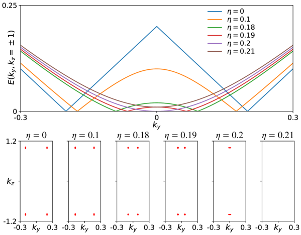
Figure A1: (Color online) Chosen parameters are $m=3$, $t=t_{z}=2$, $\lambda=1$, $\mu=0.2$, and $\Delta_{0}=\Delta_{s}=0.2$. Accordingly, $R_{\rm BIS}=\sqrt{3}$, $R_{\rm PNS}=\sqrt{2}$, and $\eta_{c}=0.2$. The $x$-normal surface band structure at $k_{z}=\pm 1$ given by Eq. (22) (top panel) and the position of four surface Bogoliubov-Dirac cones (bottom panels) for different values of $\eta$. As expected, only the $k_{y}$ coordinate of the position of the surface Bogoliubov-Dirac cones depends on $\eta$. Pairwise annihilation of the cones occurs at the critical value $\eta=0.2$.

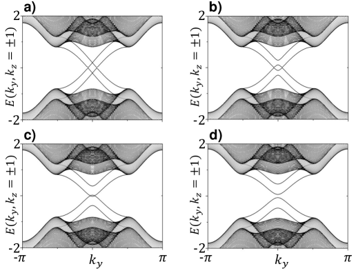
Figure A2: Energy spectrum of the full lattice Hamiltonian under open boundary conditions in the $x$ direction and periodic boundary conditions in the $y$ and $z$ directions. Chosen parameters are $m=3$, $t=t_{z}=2$, $\lambda=1$, $\mu=0.2$, and $\Delta_{0}=\Delta_{s}=0.2$. a) $\eta=0$, b) $\eta=0.1$, c) $\eta=0.2$, d) $\eta=0.3$.

Now let us consider $\eta\neq 0$. Accordingly, the surface energy spectrum becomes

$$E(k_{y},k_{z})=\pm\sqrt{\left(\sqrt{\lambda^{2}k_{y}^{2}+v_{z}^{2}(k_{y},k_{z})k_{z}^{2}}\pm\mu\right)^{2}+\frac{\Delta_{s}^{2}}{4}\left(R_{\rm BIS}^{2}-R_{\rm PNS}^{2}-\frac{t_{z}}{t}k_{z}^{2}\right)^{2}}.$$ (30)

The surface Bogoliubov-Dirac cones, if they remain, are located at a value of $k_{z}=\pm\sqrt{t(R_{\rm BIS}^{2}-R_{\rm PNS}^{2})/t_{z}}$ independent of $\eta$. The $k_{y}$ value needs to be determined by solving the equation

$$\lambda^{2}k_{y}^{2}+\eta^{2}(k_{y}^{2}+\tilde{\Delta}/\Delta_{s})^{2}t(R_{\rm BIS}^{2}-R_{\rm PNS}^{2})/t_{z}=\mu^{2},$$ (31)

or in the standard form

$$[\eta^{2}t(R_{\rm BIS}^{2}-R_{\rm PNS}^{2})/t_{z}]k_{y}^{4}$$

$$+[\lambda^{2}+2\eta^{2}(\tilde{\Delta}/\Delta_{s})t(R_{\rm BIS}^{2}-R_{\rm PNS}^{2})/t_{z}]k_{y}^{2}$$

$$+\eta^{2}(\tilde{\Delta}/\Delta_{s})^{2}t(R_{\rm BIS}^{2}-R_{\rm PNS}^{2})/t_{z}-\mu^{2}=0.$$ (32)

By defining

$$a \equiv[\eta^{2}t(R_{\rm BIS}^{2}-R_{\rm PNS}^{2})/t_{z}],$$ (33)

$$b \equiv[\lambda^{2}+2\eta^{2}(\tilde{\Delta}/\Delta_{s})t(R_{\rm BIS}^{2}-R_{\rm PNS}^{2})/t_{z}],$$ (34)

$$c \equiv\eta^{2}(\tilde{\Delta}/\Delta_{s})^{2}t(R_{\rm BIS}^{2}-R_{\rm PNS}^{2})/t_{z}-\mu^{2},$$ (35)

it is known that the solutions for $k_{y}^{2}$ take the standard form

$$k_{y}^{2}=\frac{-b\pm\sqrt{b^{2}-4ac}}{2a}.$$ (36)

There will exist gapless Bogoliubov-Dirac cones in the surface Brillouin zone as long as real and positive solutions for $k_{y}^{2}$ exist. As we are interested in the movements of the Bogoliubov-Dirac cones with the increase in $\eta$ from $0$, in the following we focus on the case with $b>0$ to give a discussion. As here the parameter $a$ is positive, the existence of a physical solution then requires $c<0$. Accordingly, one can find that the condition for the existence of gapless Bogoliubov-Dirac cones is

$$|\eta|<\eta_{c} =\frac{|\mu|\Delta_{s}}{|\tilde{\Delta}|}\sqrt{\frac{t_{z}}{t(R_{\rm BIS}^{2}-R_{\rm PNS}^{2})}}$$

$$=\frac{2|\mu|}{R_{\rm PNS}^{2}}\sqrt{\frac{t_{z}}{t(R_{\rm BIS}^{2}-R_{\rm PNS}^{2})}}.$$ (37)

Putting $\eta_{c}$ back into the formula for $b$, one obtains

$$b=\lambda^{2}+2\mu^{2}\frac{\Delta_{s}}{\tilde{\Delta}}.$$ (38)

As long as the chemical potential $|\mu|<\mu_{c}=\sqrt{|\frac{\tilde{\Delta}}{2\Delta_{s}}|}\lambda$, the parameter $b$ is positive, and the above formula for $\eta_{c}$ is valid. To intuitively see the effect of $\eta$ terms on $k_{y}^{2}$, we consider $|\mu|<\mu_{c}$ and $\eta$ to be small so that we can do an expansion in $\eta$. To second order, we find

$$k_{y}^{2}\approx\frac{\mu^{2}}{\lambda^{2}}-\frac{\eta^{2}}{\lambda^{2}}\frac{t}{t_{z}}(R_{\rm BIS}^{2}-R_{\rm PNS}^{2})\left(\frac{\tilde{\Delta}}{\Delta_{s}}\right)^{2}\left[1+\frac{\mu^{2}}{\lambda^{2}}\frac{\Delta_{s}}{\tilde{\Delta}}\right].$$ (39)

In the weakly doped regime, $\mu\ll\lambda$, one can see that the $\eta$ terms decrease the separation of surface Bogoliubov-Dirac cones in the $k_{y}$ direction, consistent with the picture that the surface Bogoliubov-Dirac cones will annihilate each other when $\eta$ is larger than a critical value. In Fig. A1, we show the evolution of the positions of surface Bogoliubov-Dirac cones with respect to $\eta$ explicitly. According to this evolution, one can find that the value at which the surface Bogoliubov-Dirac cones merge in pairs agrees with the formula for $\eta_{c}$ in Eq. (37). By diagonalizing the full lattice Hamiltonian with open boundary conditions in the $x$ direction, we find that the locations and evolution of surface Bogoliubov-Dirac cones on the $x$-normal surface agree well with the analytical analysis above, as shown in Fig. A2.

After gapping out the surface Bogoliubov-Dirac cones, we have shown both analytically and numerically that one-dimensional propagating helical Majorana modes will emerge on the hinges of a cubic sample. Here, we provide more details about the analytical derivation of the low-energy Hamiltonian for the helical Majorana hinge modes at the limit $\mu=0$. At $\mu=0$, the surface-state Hamiltonian becomes

$$H_{s}(k_{y},k_{z}) =\lambda k_{y}s_{z}-\frac{\eta k_{z}}{t}(\tilde{m}+tk_{y}^{2}+t_{z}k_{z}^{2}/2)\tau_{z}s_{y}$$

$$\quad+\frac{\Delta_{s}}{2}(R_{\rm BIS}^{2}-R_{\rm PNS}^{2}-\frac{t_{z}}{t}k_{z}^{2})\tau_{y}s_{y}.$$ (40)

It is readily found that the energy spectrum for this Hamiltonian is fully gapped as long as $\eta\neq 0$ and $R_{\rm BIS}\neq R_{\rm PNS}$. Let us focus on the small-momentum region; accordingly, we will only keep the leading momentum terms in each term of the surface-state Hamiltonian. Then the Hamiltonian reduces to

$$H_{s}(k_{y},k_{z}) =\lambda k_{y}s_{z}-\frac{\eta\tilde{m}k_{z}}{t}\tau_{z}s_{y}$$

$$\quad+\frac{\Delta_{s}}{2}(R_{\rm BIS}^{2}-R_{\rm PNS}^{2}-\frac{t_{z}}{t}k_{z}^{2})\tau_{y}s_{y}.$$ (41)

If the open boundary condition is further taken in the $z$ direction, then the Hamiltonian becomes

$$H_{s}(k_{y},-i\partial_{z}) =\lambda k_{y}s_{z}+i\frac{\eta\tilde{m}}{t}\tau_{z}s_{y}\partial_{z}$$

$$\quad+\frac{\Delta_{s}}{2}(R_{\rm BIS}^{2}-R_{\rm PNS}^{2}+\frac{t_{z}}{t}\partial_{z}^{2})\tau_{y}s_{y}.$$ (42)

As the Hamiltonian takes a form similar to $H_{0}$ in Eq.  (12), one can easily find that if we consider a half-infinity sample with the boundary at $z=0$ (the boundary is in fact a hinge as it corresponds to the boundary of a surface), there exist two solutions satisfying the eigenvalue equation $H_{s}\phi_{\alpha}(z)=E_{\alpha}\phi_{\alpha}(z)$ and the boundary condition $\phi_{\alpha}(0)=\phi_{\alpha}(\infty)=0$. The expressions for the two solutions are similar to those in Eq. (14),

$$\phi_{\alpha}(z)=\mathcal{N}^{\prime}\sin(\kappa^{\prime}_{1}z)e^{-(\kappa^{\prime}_{2}z)}e^{ik_{y}y}\chi_{\alpha}^{\prime},$$ (43)

where the normalization constant is given by $\mathcal{N}^{\prime}=2\sqrt{\kappa_{2}^{\prime}(\kappa_{1}^{{}^{\prime}2}+\kappa_{2}^{{}^{\prime}2})/\kappa_{1}^{{}^{\prime}2}}$, with

$$\kappa_{1}^{\prime} =\sqrt{\frac{t(R_{\rm BIS}^{2}-R_{\rm PNS}^{2})}{t_{z}}-\left(\frac{\eta\tilde{m}}{t_{z}\Delta_{s}}\right)^{2}},$$ (44)

$$\kappa_{2}^{\prime} =-\frac{\eta\tilde{m}}{t_{z}\Delta_{s}}.$$ (45)

The normalization of the wave functions requires $R_{\rm BIS}^{2}>R_{\rm PNS}^{2}$, indicating that the crossing of the BIS and PNS is a precondition for the realization of the helical Majorana hinge modes. Here the two spinors $\chi_{\alpha}^{\prime}$ can be chosen as $\chi_{1}^{\prime}=|\tau_{x}=1,s_{z}=1\rangle$ and $\chi_{2}^{\prime}=|\tau_{x}=1,s_{z}=-1\rangle$. Correspondingly, $E_{1}=\lambda k_{y}$ and $E_{2}=-\lambda k_{y}$. As the two spinors indicate that each branch of the hinge states is spin-polarized and an equal superposition of electron and hole, this analysis confirms that the two branches of hinge states correspond to a pair of helical Majorana modes. In the basis $(\phi_{1},\phi_{2})^{T}$, the low-energy Hamiltonian that describes the helical Majorana hinge modes reads

$$H_{h}(k_{y})=\lambda k_{y}s_{z}.$$ (46)

Appendix B Importance of $\eta$ terms for the realization of first-order time-reversal invariant topological superconductivity in thin films of superconducting Dirac semimetal

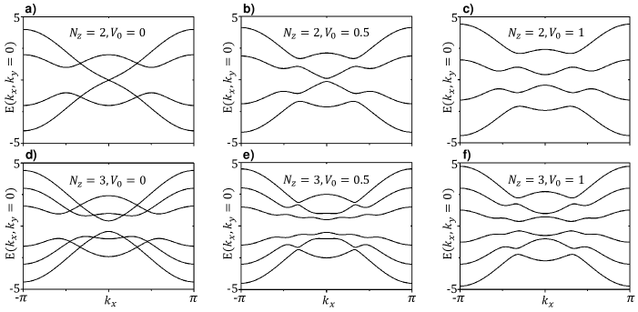
Figure B1: The evolution of normal-state energy spectra with respect to gate potential for bilayer and trilayer thin films. Chosen parameters are $m=3$, $t=t_{z}=2$, $\lambda=1$, and $\eta=0$. The gate voltage cannot lift the spin degeneracy when the $\eta$ terms are absent.

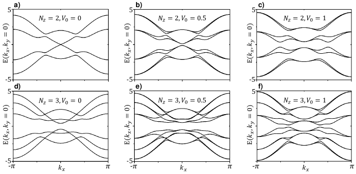
Figure B2: The evolution of normal-state energy spectra with respect to gate potential for bilayer and trilayer thin films. Chosen parameters are $m=3$, $t=t_{z}=2$, $\lambda=1$, and $\eta=1$. The gate voltage lifts the spin degeneracy when the $\eta$ terms are finite.

In this appendix, we will show that the $\eta$ terms are also crucial for the realization of first-order time-reversal invariant topological superconductivity in thin films of the superconducting Dirac semimetal. Before proceeding, we recall the fact that, for the even-parity pairing discussed here, lifting the spin degeneracy of the Fermi surface is a precondition for the realization of first-order time-reversal invariant topological superconductivity in two dimensions.

We first investigate the energy spectrum of thin-film Dirac semimetals when $\eta=0$ and superconductivity is absent. To be specific, here we focus on thin films with number of layers $N_{z}=2$ and $N_{z}=3$. We find that, for both the bilayer and trilayer, while the gate voltage can strongly modify the dispersions of the energy bands, it cannot lift the spin degeneracy, as shown in Fig. B1. Since the double degeneracy of the energy bands cannot be lifted by the gate voltage, this suggests that when the $\eta$ terms are absent, the naive approach of using gate voltage to drive the superconducting Dirac semimetal with even-parity pairing into a first-order time-reversal invariant topological superconductor does not work.

For comparison, we change $\eta$ from $0$ to $1$ and keep other parameters fixed, with the corresponding energy bands shown in Fig. B2. One can see that, for both the bilayer and the trilayer thin films, the double degeneracy of energy bands is lifted by a finite gate voltage, which makes the realization of first-order time-reversal invariant topological superconductivity possible.

To understand the origin of the qualitative difference between the two situations with and without the $\eta$ terms, here we take the bilayer case for illustration. When $N_{z}=2$, in the basis $(c_{a,\uparrow,k_{x},k_{y},z=1}^{{\dagger}},c_{b,\uparrow,k_{x},k_{y},z=1}^{{\dagger}},c_{a,\downarrow,k_{x},k_{y},z=1}^{{\dagger}},c_{b,\downarrow,k_{x},k_{y},z=1}^{{\dagger}},\\ c_{a,\uparrow,k_{x},k_{y},z=2}^{{\dagger}},c_{b,\uparrow,k_{x},k_{y},z=2}^{{\dagger}},c_{a,\downarrow,k_{x},k_{y},z=2}^{{\dagger}},c_{b,\downarrow,k_{x},k_{y},z=2}^{{\dagger}})$, the normal-state Hamiltonian can be written as

$$H(\bm{k}) =(m-t\cos k_{x}-t\cos k_{y})\sigma_{z}-\frac{t_{z}}{2}\rho_{x}\sigma_{z}$$

$$\quad+\lambda(\sin k_{x}s_{z}\sigma_{x}-\sin k_{y}\sigma_{y})+\eta\sin k_{x}\sin k_{y}\rho_{y}s_{y}\sigma_{x}$$

$$\quad+\frac{\eta}{2}(\cos k_{x}-\cos k_{y})\rho_{y}s_{x}\sigma_{x}+V_{0}\rho_{z},$$ (47)

where the Pauli matrices $\sigma_{i}$, $s_{i}$, and $\rho_{i}$ act on orbital, spin, and layer degrees of freedom, respectively. When $\eta=0$, although the physical inversion symmetry (the inversion symmetry operator becomes $\tilde{I}=\rho_{x}\sigma_{z}$ as it should exchange the two layers) is broken, one finds that the Hamiltonian still commutes with the antiunitary operator $is_{y}\mathcal{K}\sigma_{z}$ which is a combination of time-reversal and inversion symmetry in orbital space. The combined symmetry obeys $(is_{y}\mathcal{K}\sigma_{z})^{2}=-1$, and the energy bands thus still obey Kramers’ degeneracy at each $\bm{k}$. However, once $\eta\neq 0$, the two $\eta$ terms are odd under that combined symmetry, and lead to a splitting of Kramers’ degeneracy.

References

- Read and Green (2000) N. Read and Dmitry Green, “Paired states of fermions in two dimensions with breaking of parity and time-reversal symmetries and the fractional quantum Hall effect,” Phys. Rev. B 61, 10267–10297 (2000).
- Kitaev (2001) Alexei Kitaev, “Unpaired Majorana fermions in quantum wires,” Physics-Uspekhi 44, 131 (2001).
- Alicea (2012) Jason Alicea, “New directions in the pursuit of Majorana fermions in solid state systems,” Reports on Progress in Physics 75, 076501 (2012).
- Leijnse and Flensberg (2012) Martin Leijnse and Karsten Flensberg, “Introduction to topological superconductivity and Majorana fermions,” Semiconductor Science and Technology 27, 124003 (2012).
- Beenakker (2013) C. W. J. Beenakker, “Search for Majorana Fermions in Superconductors,” Annual Review of Condensed Matter Physics 4, 113–136 (2013).
- Stanescu and Tewari (2013) Tudor D Stanescu and Sumanta Tewari, “Majorana fermions in semiconductor nanowires: fundamentals, modeling, and experiment,” Journal of Physics: Condensed Matter 25, 233201 (2013).
- Elliott and Franz (2015) Steven R. Elliott and Marcel Franz, “Colloquium : Majorana fermions in nuclear, particle, and solid-state physics,” Rev. Mod. Phys. 87, 137–163 (2015).
- Sato and Fujimoto (2016) Masatoshi Sato and Satoshi Fujimoto, “Majorana fermions and topology in superconductors,” Journal of the Physical Society of Japan 85, 072001 (2016).
- Aguado (2017) Ramón Aguado, “Majorana quasiparticles in condensed matter,” La Rivista del Nuovo Cimento 40, 523–593 (2017).
- Haim and Oreg (2019) Arbel Haim and Yuval Oreg, “Time-reversal-invariant topological superconductivity in one and two dimensions,” Physics Reports 825, 1–48 (2019).
- Jäck et al. (2021) Berthold Jäck, Yonglong Xie, and Ali Yazdani, “Detecting and distinguishing Majorana zero modes with the scanning tunneling microscope,” arXiv preprint arXiv:2103.13210 (2021).
- Ivanov (2001) D. A. Ivanov, “Non-Abelian statistics of half-quantum vortices in -wave superconductors,” Phys. Rev. Lett. 86, 268–271 (2001).
- Alicea et al. (2011) Jason Alicea, Yuval Oreg, Gil Refael, Felix von Oppen, and Matthew P. A. Fisher, “Non-Abelian statistics and topological quantum information processing in 1D wire networks,” Nature Physics 7, 412–417 (2011).
- Nayak et al. (2008) Chetan Nayak, Steven H. Simon, Ady Stern, Michael Freedman, and Sankar Das Sarma, “Non-Abelian anyons and topological quantum computation,” Rev. Mod. Phys. 80, 1083–1159 (2008).
- Sarma et al. (2015) Sankar Das Sarma, Michael Freedman, and Chetan Nayak, “Majorana zero modes and topological quantum computation,” npj Quantum Information 1, 15001 (2015).
- Benalcazar et al. (2017a) Wladimir A. Benalcazar, B. Andrei Bernevig, and Taylor L. Hughes, “Quantized electric multipole insulators,” Science 357, 61–66 (2017a).
- Schindler et al. (2018) Frank Schindler, Ashley M. Cook, Maia G. Vergniory, Zhijun Wang, Stuart S. P. Parkin, B. Andrei Bernevig, and Titus Neupert, “Higher-order topological insulators,” Science Advances 4 (2018), 10.1126/sciadv.aat0346.
- Benalcazar et al. (2017b) Wladimir A. Benalcazar, B. Andrei Bernevig, and Taylor L. Hughes, “Electric multipole moments, topological multipole moment pumping, and chiral hinge states in crystalline insulators,” Phys. Rev. B 96, 245115 (2017b).
- Song et al. (2017) Zhida Song, Zhong Fang, and Chen Fang, “-dimensional edge states of rotation symmetry protected topological states,” Phys. Rev. Lett. 119, 246402 (2017).
- Langbehn et al. (2017) J. Langbehn, Yang Peng, L. Trifunovic, Felix von Oppen, and Piet W. Brouwer, “Reflection-symmetric second-order topological insulators and superconductors,” Phys. Rev. Lett. 119, 246401 (2017).
- Khalaf (2018) Eslam Khalaf, “Higher-order topological insulators and superconductors protected by inversion symmetry,” Phys. Rev. B 97, 205136 (2018).
- Geier et al. (2018) Max Geier, Luka Trifunovic, Max Hoskam, and Piet W. Brouwer, “Second-order topological insulators and superconductors with an order-two crystalline symmetry,” Phys. Rev. B 97, 205135 (2018).
- Zhu (2018) Xiaoyu Zhu, “Tunable Majorana corner states in a two-dimensional second-order topological superconductor induced by magnetic fields,” Phys. Rev. B 97, 205134 (2018).
- Yan et al. (2018) Zhongbo Yan, Fei Song, and Zhong Wang, “Majorana corner modes in a high-temperature platform,” Phys. Rev. Lett. 121, 096803 (2018).
- Wang et al. (2018a) Qiyue Wang, Cheng-Cheng Liu, Yuan-Ming Lu, and Fan Zhang, “High-temperature Majorana corner states,” Phys. Rev. Lett. 121, 186801 (2018a).
- Wang et al. (2018b) Yuxuan Wang, Mao Lin, and Taylor L. Hughes, “Weak-pairing higher order topological superconductors,” Phys. Rev. B 98, 165144 (2018b).
- Yan (2019a) Zhongbo Yan, “Higher-order topological odd-parity superconductors,” Phys. Rev. Lett. 123, 177001 (2019a).
- Shapourian et al. (2018) Hassan Shapourian, Yuxuan Wang, and Shinsei Ryu, “Topological crystalline superconductivity and second-order topological superconductivity in nodal-loop materials,” Phys. Rev. B 97, 094508 (2018).
- Hsu et al. (2018) Chen-Hsuan Hsu, Peter Stano, Jelena Klinovaja, and Daniel Loss, “Majorana Kramers pairs in higher-order topological insulators,” Phys. Rev. Lett. 121, 196801 (2018).
- Liu et al. (2018a) Tao Liu, James Jun He, and Franco Nori, “Majorana corner states in a two-dimensional magnetic topological insulator on a high-temperature superconductor,” Phys. Rev. B 98, 245413 (2018a).
- Wu et al. (2019) Zhigang Wu, Zhongbo Yan, and Wen Huang, “Higher-order topological superconductivity: Possible realization in Fermi gases and \ceSr2RuO4,” Phys. Rev. B 99, 020508 (2019).
- Zhang et al. (2019a) Rui-Xing Zhang, William S. Cole, and S. Das Sarma, “Helical hinge Majorana modes in iron-based superconductors,” Phys. Rev. Lett. 122, 187001 (2019a).
- Zhang et al. (2019b) Rui-Xing Zhang, William S. Cole, Xianxin Wu, and S. Das Sarma, “Higher-order topology and nodal topological superconductivity in Fe(Se,Te) heterostructures,” Phys. Rev. Lett. 123, 167001 (2019b).
- Volpez et al. (2019) Yanick Volpez, Daniel Loss, and Jelena Klinovaja, “Second-order topological superconductivity in -junction Rashba layers,” Phys. Rev. Lett. 122, 126402 (2019).
- Zhu (2019) Xiaoyu Zhu, “Second-order topological superconductors with mixed pairing,” Phys. Rev. Lett. 122, 236401 (2019).
- Peng and Xu (2019) Yang Peng and Yong Xu, “Proximity-induced Majorana hinge modes in antiferromagnetic topological insulators,” Phys. Rev. B 99, 195431 (2019).
- Ghorashi et al. (2019) Sayed Ali Akbar Ghorashi, Xiang Hu, Taylor L. Hughes, and Enrico Rossi, “Second-order Dirac superconductors and magnetic field induced Majorana hinge modes,” Phys. Rev. B 100, 020509 (2019).
- Yan (2019b) Zhongbo Yan, “Majorana corner and hinge modes in second-order topological insulator/superconductor heterostructures,” Phys. Rev. B 100, 205406 (2019b).
- Bultinck et al. (2019) Nick Bultinck, B. Andrei Bernevig, and Michael P. Zaletel, “Three-dimensional superconductors with hybrid higher-order topology,” Phys. Rev. B 99, 125149 (2019).
- Franca et al. (2019) S. Franca, D. V. Efremov, and I. C. Fulga, “Phase-tunable second-order topological superconductor,” Phys. Rev. B 100, 075415 (2019).
- Pan et al. (2019) Xiao-Hong Pan, Kai-Jie Yang, Li Chen, Gang Xu, Chao-Xing Liu, and Xin Liu, “Lattice-symmetry-assisted second-order topological superconductors and Majorana patterns,” Phys. Rev. Lett. 123, 156801 (2019).
- Kheirkhah et al. (2020a) Majid Kheirkhah, Yuki Nagai, Chun Chen, and Frank Marsiglio, “Majorana corner flat bands in two-dimensional second-order topological superconductors,” Phys. Rev. B 101, 104502 (2020a).
- Kheirkhah et al. (2020b) Majid Kheirkhah, Zhongbo Yan, Yuki Nagai, and Frank Marsiglio, “First- and second-order topological superconductivity and temperature-driven topological phase transitions in the extended Hubbard model with spin-orbit coupling,” Phys. Rev. Lett. 125, 017001 (2020b).
- Wu et al. (2020a) Ya-Jie Wu, Junpeng Hou, Yun-Mei Li, Xi-Wang Luo, Xiaoyan Shi, and Chuanwei Zhang, “In-plane Zeeman-field-induced Majorana corner and hinge modes in an -wave superconductor heterostructure,” Phys. Rev. Lett. 124, 227001 (2020a).
- Hsu et al. (2020) Yi-Ting Hsu, William S. Cole, Rui-Xing Zhang, and Jay D. Sau, “Inversion-protected higher-order topological superconductivity in monolayer \ceWTe2,” Phys. Rev. Lett. 125, 097001 (2020).
- Wu et al. (2020b) Xianxin Wu, Wladimir A. Benalcazar, Yinxiang Li, Ronny Thomale, Chao-Xing Liu, and Jiangping Hu, “Boundary-obstructed topological high-Tc superconductivity in iron pnictides,” Phys. Rev. X 10, 041014 (2020b).
- Laubscher et al. (2020) Katharina Laubscher, Danial Chughtai, Daniel Loss, and Jelena Klinovaja, “Kramers pairs of Majorana corner states in a topological insulator bilayer,” Phys. Rev. B 102, 195401 (2020).
- Tiwari et al. (2020) Apoorv Tiwari, Ammar Jahin, and Yuxuan Wang, “Chiral Dirac superconductors: Second-order and boundary-obstructed topology,” Phys. Rev. Research 2, 043300 (2020).
- Ahn and Yang (2020) Junyeong Ahn and Bohm-Jung Yang, “Higher-order topological superconductivity of spin-polarized fermions,” Phys. Rev. Research 2, 012060 (2020).
- Roy (2020) Bitan Roy, “Higher-order topological superconductors in -, -odd quadrupolar Dirac materials,” Phys. Rev. B 101, 220506 (2020).
- Li and Yan (2021) Bo-Xuan Li and Zhongbo Yan, “Boundary topological superconductors,” Phys. Rev. B 103, 064512 (2021).
- Niu et al. (2021) Jingjing Niu, Tongxing Yan, Yuxuan Zhou, Ziyu Tao, Xiaole Li, Weiyang Liu, Libo Zhang, Hao Jia, Song Liu, Zhongbo Yan, et al., “Simulation of higher-order topological phases and related topological phase transitions in a superconducting qubit,” Science Bulletin 66, 1168–1175 (2021).
- Wu et al. (2021a) Xianxin Wu, Xin Liu, Ronny Thomale, and Chao-Xing Liu, “High-Tc superconductor Fe(Se,Te) Monolayer: an intrinsic, scalable and electrically-tunable Majorana platform,” National Science Review , 2095–5138 (2021a).
- Fu et al. (2021) Bo Fu, Zi-Ang Hu, Chang-An Li, Jian Li, and Shun-Qing Shen, “Chiral Majorana hinge modes in superconducting Dirac materials,” Phys. Rev. B 103, L180504 (2021).
- Luo et al. (2021) Xun-Jiang Luo, Xiao-Hong Pan, and Xin Liu, “Higher-order topological superconductors based on weak topological insulators,” arXiv preprint arXiv:2103.01825 (2021).
- Jahin et al. (2021) Ammar Jahin, Apoorv Tiwari, and Yuxuan Wang, “Higher-order topological superconductors from Weyl semimetals,” arXiv preprint arXiv:2103.05010 (2021).
- Qin et al. (2021) Shengshan Qin, Chen Fang, Fu-Chun Zhang, and Jiangping Hu, “Topological superconductivity in an -wave superconductor and its implication to iron-based superconductors,” arXiv preprint arXiv:2106.04200 (2021).
- Tan et al. (2021) Yi Tan, Zhi-Hao Huang, and Xiong-Jun Liu, “Edge geometric phase mechanism for second-order topological insulator and superconductor,” arXiv preprint arXiv:2106.12507 (2021).
- You et al. (2019) Yizhi You, Daniel Litinski, and Felix von Oppen, “Higher-order topological superconductors as generators of quantum codes,” Phys. Rev. B 100, 054513 (2019).
- Zhang et al. (2020a) Song-Bo Zhang, Alessio Calzona, and Björn Trauzettel, “All-electrically tunable networks of Majorana bound states,” Phys. Rev. B 102, 100503 (2020a).
- Zhang et al. (2020b) Song-Bo Zhang, W. B. Rui, Alessio Calzona, Sang-Jun Choi, Andreas P. Schnyder, and Björn Trauzettel, “Topological and holonomic quantum computation based on second-order topological superconductors,” Phys. Rev. Research 2, 043025 (2020b).
- Pahomi et al. (2020) Tudor E. Pahomi, Manfred Sigrist, and Alexey A. Soluyanov, “Braiding Majorana corner modes in a second-order topological superconductor,” Phys. Rev. Research 2, 032068 (2020).
- Bomantara and Gong (2020) Raditya Weda Bomantara and Jiangbin Gong, “Measurement-only quantum computation with Floquet Majorana corner modes,” Phys. Rev. B 101, 085401 (2020).
- Lapa et al. (2021) Matthew F Lapa, Meng Cheng, and Yuxuan Wang, “Symmetry-protected gates of Majorana qubits in a high-Tc superconductor platform,” arXiv preprint arXiv:2103.03893 (2021).
- Ikegaya et al. (2021) S. Ikegaya, W. B. Rui, D. Manske, and Andreas P. Schnyder, “Tunable Majorana corner modes in noncentrosymmetric superconductors: Tunneling spectroscopy and edge imperfections,” Phys. Rev. Research 3, 023007 (2021).
- Roy and Juricic (2021) Bitan Roy and Vladimir Juricic, “Mixed parity octupolar pairing and corner Majorana modes in three dimensions,” arXiv preprint arXiv:2106.01361 (2021).
- Fu and Kane (2008) Liang Fu and C. L. Kane, “Superconducting proximity effect and Majorana fermions at the surface of a topological insulator,” Phys. Rev. Lett. 100, 096407 (2008).
- Lutchyn et al. (2011) Roman M. Lutchyn, Tudor D. Stanescu, and S. Das Sarma, “Search for Majorana fermions in multiband semiconducting nanowires,” Phys. Rev. Lett. 106, 127001 (2011).
- Oreg et al. (2010) Yuval Oreg, Gil Refael, and Felix von Oppen, “Helical liquids and Majorana bound states in quantum wires,” Phys. Rev. Lett. 105, 177002 (2010).
- Sau et al. (2010) Jay D. Sau, Roman M. Lutchyn, Sumanta Tewari, and S. Das Sarma, “Generic new platform for topological quantum computation using semiconductor heterostructures,” Phys. Rev. Lett. 104, 040502 (2010).
- Alicea (2010) Jason Alicea, “Majorana fermions in a tunable semiconductor device,” Phys. Rev. B 81, 125318 (2010).
- Mourik et al. (2012) V. Mourik, K. Zuo, S. M. Frolov, S. R. Plissard, E. P. A. M. Bakkers, and L. P. Kouwenhoven, “Signatures of Majorana fermions in hybrid superconductor-semiconductor nanowire devices,” Science 336, 1003–1007 (2012).
- Rokhinson et al. (2012) Leonid P Rokhinson, Xinyu Liu, and Jacek K Furdyna, “The fractional ac Josephson effect in a semiconductor-superconductor nanowire as a signature of Majorana particles,” Nature Physics 8, 795–799 (2012).
- Das et al. (2012) Anindya Das, Yuval Ronen, Yonatan Most, Yuval Oreg, Moty Heiblum, and Hadas Shtrikman, “Zero-bias peaks and splitting in an Al-InAs nanowire topological superconductor as a signature of Majorana fermions,” Nature Physics 8, 887–895 (2012).
- Deng et al. (2012) MT Deng, CL Yu, GY Huang, Marcus Larsson, Philippe Caroff, and HQ Xu, “Anomalous zero-bias conductance peak in a Nb–InSb nanowire–Nb hybrid device,” Nano letters 12, 6414–6419 (2012).
- Finck et al. (2013) A. D. K. Finck, D. J. Van Harlingen, P. K. Mohseni, K. Jung, and X. Li, “Anomalous modulation of a zero-bias peak in a hybrid nanowire-superconductor device,” Phys. Rev. Lett. 110, 126406 (2013).
- Nadj-Perge et al. (2014) Stevan Nadj-Perge, Ilya K Drozdov, Jian Li, Hua Chen, Sangjun Jeon, Jungpil Seo, Allan H MacDonald, B Andrei Bernevig, and Ali Yazdani, “Observation of Majorana fermions in ferromagnetic atomic chains on a superconductor,” Science 346, 602–607 (2014).
- Sun et al. (2016) Hao-Hua Sun, Kai-Wen Zhang, Lun-Hui Hu, Chuang Li, Guan-Yong Wang, Hai-Yang Ma, Zhu-An Xu, Chun-Lei Gao, Dan-Dan Guan, Yao-Yi Li, Canhua Liu, Dong Qian, Yi Zhou, Liang Fu, Shao-Chun Li, Fu-Chun Zhang, and Jin-Feng Jia, “Majorana zero mode detected with spin selective Andreev reflection in the vortex of a topological superconductor,” Phys. Rev. Lett. 116, 257003 (2016).
- Deng et al. (2016) MT Deng, S Vaitiekėnas, EB Hansen, J Danon, M Leijnse, K Flensberg, J Nygård, P Krogstrup, and CM Marcus, “Majorana bound state in a coupled quantum-dot hybrid-nanowire system,” Science 354, 1557–1562 (2016).
- Fornieri et al. (2019) Antonio Fornieri, Alexander M. Whiticar, F. Setiawan, Elías Portolés, Asbjørn C. C. Drachmann, Anna Keselman, Sergei Gronin, Candice Thomas, Tian Wang, Ray Kallaher, Geoffrey C. Gardner, Erez Berg, Michael J. Manfra, Ady Stern, Charles M. Marcus, and Fabrizio Nichele, “Evidence of topological superconductivity in planar Josephson junctions,” Nature 569, 89–92 (2019).
- Ren et al. (2019) Hechen Ren, Falko Pientka, Sean Hart, Andrew T. Pierce, Michael Kosowsky, Lukas Lunczer, Raimund Schlereth, Benedikt Scharf, Ewelina M. Hankiewicz, Laurens W. Molenkamp, Bertrand I. Halperin, and Amir Yacoby, “Topological superconductivity in a phase-controlled Josephson junction,” Nature 569, 93–98 (2019).
- Zhang et al. (2019c) Hao Zhang, Dong E. Liu, Michael Wimmer, and Leo P. Kouwenhoven, “Next steps of quantum transport in Majorana nanowire devices,” Nature Communications 10, 5128 (2019c).
- Frolov et al. (2020) S. M. Frolov, M. J. Manfra, and J. D. Sau, “Topological superconductivity in hybrid devices,” Nature Physics 16, 718–724 (2020).
- Yu et al. (2021) P. Yu, J. Chen, M. Gomanko, G. Badawy, E. P. A. M. Bakkers, K. Zuo, V. Mourik, and S. M. Frolov, “Non-Majorana states yield nearly quantized conductance in proximatized nanowires,” Nature Physics 17, 482–488 (2021).
- Zhang et al. (2018) Peng Zhang, Koichiro Yaji, Takahiro Hashimoto, Yuichi Ota, Takeshi Kondo, Kozo Okazaki, Zhijun Wang, Jinsheng Wen, GD Gu, Hong Ding, et al., “Observation of topological superconductivity on the surface of an iron-based superconductor,” Science 360, 182–186 (2018).
- Zhang et al. (2019d) Peng Zhang, Zhijun Wang, Xianxin Wu, Koichiro Yaji, Yukiaki Ishida, Yoshimitsu Kohama, Guangyang Dai, Yue Sun, Cedric Bareille, Kenta Kuroda, et al., “Multiple topological states in iron-based superconductors,” Nature Physics 15, 41 (2019d).
- Wang et al. (2018c) Dongfei Wang, Lingyuan Kong, Peng Fan, Hui Chen, Shiyu Zhu, Wenyao Liu, Lu Cao, Yujie Sun, Shixuan Du, John Schneeloch, et al., “Evidence for Majorana bound states in an iron-based superconductor,” Science 362, 333–335 (2018c).
- Liu et al. (2018b) Qin Liu, Chen Chen, Tong Zhang, Rui Peng, Ya-Jun Yan, Chen-Hao-Ping Wen, Xia Lou, Yu-Long Huang, Jin-Peng Tian, Xiao-Li Dong, Guang-Wei Wang, Wei-Cheng Bao, Qiang-Hua Wang, Zhi-Ping Yin, Zhong-Xian Zhao, and Dong-Lai Feng, “Robust and clean Majorana zero mode in the vortex core of high-temperature superconductor \ce(Li_0.84Fe_0.16)OHFeSe,” Phys. Rev. X 8, 041056 (2018b).
- Machida et al. (2019) T Machida, Y Sun, S Pyon, S Takeda, Y Kohsaka, T Hanaguri, T Sasagawa, and T Tamegai, “Zero-energy vortex bound state in the superconducting topological surface state of Fe(Se, Te),” Nature materials 18, 811–815 (2019).
- Kong et al. (2019) Lingyuan Kong, Shiyu Zhu, Michał Papaj, Hui Chen, Lu Cao, Hiroki Isobe, Yuqing Xing, Wenyao Liu, Dongfei Wang, Peng Fan, et al., “Half-integer level shift of vortex bound states in an iron-based superconductor,” Nature Physics 15, 1181–1187 (2019).
- Zhu et al. (2020) Shiyu Zhu, Lingyuan Kong, Lu Cao, Hui Chen, Michał Papaj, Shixuan Du, Yuqing Xing, Wenyao Liu, Dongfei Wang, Chengmin Shen, Fazhi Yang, John Schneeloch, Ruidan Zhong, Genda Gu, Liang Fu, Yu-Yang Zhang, Hong Ding, and Hong-Jun Gao, “Nearly quantized conductance plateau of vortex zero mode in an iron-based superconductor,” Science 367, 189–192 (2020).
- Jiang et al. (2019) Kun Jiang, Xi Dai, and Ziqiang Wang, “Quantum anomalous vortex and Majorana zero mode in iron-based superconductor Fe(Te,Se),” Phys. Rev. X 9, 011033 (2019).
- Qin et al. (2019a) Shengshan Qin, Lunhui Hu, Xianxin Wu, Xia Dai, Chen Fang, Fu-Chun Zhang, and Jiangping Hu, “Topological vortex phase transitions in iron-based superconductors,” Science Bulletin 64, 1207 – 1214 (2019a).
- Chiu et al. (2020) Ching-Kai Chiu, T Machida, Yingyi Huang, T Hanaguri, and Fu-Chun Zhang, “Scalable Majorana vortex modes in iron-based superconductors,” Science Advances 6, eaay0443 (2020).
- Ghazaryan et al. (2020) Areg Ghazaryan, P. L. S. Lopes, Pavan Hosur, Matthew J. Gilbert, and Pouyan Ghaemi, “Effect of zeeman coupling on the Majorana vortex modes in iron-based topological superconductors,” Phys. Rev. B 101, 020504 (2020).
- Wu et al. (2021b) Xianxin Wu, Suk Bum Chung, Chaoxing Liu, and Eun-Ah Kim, “Topological orders competing for the Dirac surface state in \ceFeSeTe surfaces,” Phys. Rev. Research 3, 013066 (2021b).
- Kheirkhah et al. (2021) Majid Kheirkhah, Zhongbo Yan, and Frank Marsiglio, “Vortex-line topology in iron-based superconductors with and without second-order topology,” Phys. Rev. B 103, L140502 (2021).
- Qin et al. (2019b) Shengshan Qin, Lunhui Hu, Congcong Le, Jinfeng Zeng, Fu-chun Zhang, Chen Fang, and Jiangping Hu, “Quasi-1D topological nodal vortex line phase in doped superconducting 3D Dirac semimetals,” Phys. Rev. Lett. 123, 027003 (2019b).
- König and Coleman (2019) Elio J. König and Piers Coleman, “Crystalline-Symmetry-Protected Helical Majorana Modes in the Iron Pnictides,” Phys. Rev. Lett. 122, 207001 (2019).
- Yan et al. (2020) Zhongbo Yan, Zhigang Wu, and Wen Huang, “Vortex end Majorana zero modes in superconducting Dirac and Weyl semimetals,” Phys. Rev. Lett. 124, 257001 (2020).
- Kawakami and Sato (2019) Takuto Kawakami and Masatoshi Sato, “Topological crystalline superconductivity in Dirac semimetal phase of iron-based superconductors,” Phys. Rev. B 100, 094520 (2019).
- Yang and Nagaosa (2014) Bohm-Jung Yang and Naoto Nagaosa, “Classification of stable three-dimensional Dirac semimetals with nontrivial topology,” Nature Communications 5, 4898 (2014).
- Kobayashi and Sato (2015) Shingo Kobayashi and Masatoshi Sato, “Topological superconductivity in Dirac semimetals,” Phys. Rev. Lett. 115, 187001 (2015).
- Kargarian et al. (2016) Mehdi Kargarian, Mohit Randeria, and Yuan-Ming Lu, “Are the surface Fermi arcs in Dirac semimetals topologically protected?” Proceedings of the National Academy of Sciences 113, 8648–8652 (2016).
- Wieder et al. (2020) Benjamin J. Wieder, Zhijun Wang, Jennifer Cano, Xi Dai, Leslie M. Schoop, Barry Bradlyn, and B. Andrei Bernevig, “Strong and fragile topological Dirac semimetals with higher-order Fermi arcs,” Nature Communications 11, 627 (2020).
- Le et al. (2018) Congcong Le, Xianxin Wu, Shengshan Qin, Yinxiang Li, Ronny Thomale, Fu-Chun Zhang, and Jiangping Hu, “Dirac semimetal in -CuI without surface fermi arcs,” Proceedings of the National Academy of Sciences 115, 8311–8315 (2018).
- Schnyder et al. (2008) Andreas P. Schnyder, Shinsei Ryu, Akira Furusaki, and Andreas W. W. Ludwig, “Classification of topological insulators and superconductors in three spatial dimensions,” Phys. Rev. B 78, 195125 (2008).
- Kitaev (2009) Alexei Kitaev, “Periodic table for topological insulators and superconductors,” in AIP Conference Proceedings, Vol. 1134 (AIP, 2009) pp. 22–30.
- Roy (2008) Rahul Roy, “Topological superfluids with time reversal symmetry,” arXiv:0803.2868 (2008).
- Qi et al. (2009) Xiao-Liang Qi, Taylor L. Hughes, S. Raghu, and Shou-Cheng Zhang, “Time-reversal-invariant topological superconductors and superfluids in two and three dimensions,” Phys. Rev. Lett. 102, 187001 (2009).
- Volovik (2009) G. E. Volovik, “Fermion zero modes at the boundary of superfluid 3He-B,” JETP Lett. 90, 398–401 (2009).
- Qi et al. (2010) Xiao-Liang Qi, Taylor L. Hughes, and Shou-Cheng Zhang, “Topological invariants for the fermi surface of a time-reversal-invariant superconductor,” Phys. Rev. B 81, 134508 (2010).
- Haldane (2014) FDM Haldane, “Attachment of Surface “Fermi Arcs” to the Bulk Fermi Surface: “Fermi-Level Plumbing” in Topological Metals,” arXiv preprint arXiv:1401.0529 (2014).
- Ryu et al. (2010) Shinsei Ryu, Andreas Schnyder, Akira Furusaki, and Andreas Ludwig, “Topological insulators and superconductors: ten-fold way and dimensional hierarchy,” New J. Phys. 12, 065010 (2010).
- Shen (2013) Shun-Qing Shen, Topological Insulators: Dirac Equation in Condensed Matters, Vol. 174 (Springer Science & Business Media, 2013).
- Zhang and Das Sarma (2021) Rui-Xing Zhang and S. Das Sarma, “Intrinsic time-reversal-invariant topological superconductivity in thin films of iron-based superconductors,” Phys. Rev. Lett. 126, 137001 (2021).
- Nakosai et al. (2012) Sho Nakosai, Yukio Tanaka, and Naoto Nagaosa, “Topological superconductivity in bilayer Rashba system,” Phys. Rev. Lett. 108, 147003 (2012).
- Zhang et al. (2013) Fan Zhang, C. L. Kane, and E. J. Mele, “Time-reversal-invariant topological superconductivity and Majorana Kramers pairs,” Phys. Rev. Lett. 111, 056402 (2013).
- Wang et al. (2014) Jing Wang, Yong Xu, and Shou-Cheng Zhang, “Two-dimensional time-reversal-invariant topological superconductivity in a doped quantum spin-Hall insulator,” Phys. Rev. B 90, 054503 (2014).
- Parhizgar and Black-Schaffer (2017) Fariborz Parhizgar and Annica M. Black-Schaffer, “Highly tunable time-reversal-invariant topological superconductivity in topological insulator thin films,” Scientific Reports 7, 9817 (2017).
- Casas et al. (2019) Oscar E. Casas, Liliana Arrachea, William J. Herrera, and Alfredo Levy Yeyati, “Proximity induced time-reversal topological superconductivity in \ceBi2Se3 films without phase tuning,” Phys. Rev. B 99, 161301 (2019).
- Kezilebieke et al. (2020) Shawulienu Kezilebieke, Md Nurul Huda, Viliam Vaňo, Markus Aapro, Somesh C. Ganguli, Orlando J. Silveira, Szczepan Głodzik, Adam S. Foster, Teemu Ojanen, and Peter Liljeroth, “Topological superconductivity in a van der Waals heterostructure,” Nature 588, 424–428 (2020).
- Gray et al. (2019) Mason J. Gray, Josef Freudenstein, Shu Yang F. Zhao, Ryan O’Connor, Samuel Jenkins, Narendra Kumar, Marcel Hoek, Abigail Kopec, Soonsang Huh, Takashi Taniguchi, Kenji Watanabe, Ruidan Zhong, Changyoung Kim, G. D. Gu, and K. S. Burch, “Evidence for helical hinge zero modes in an Fe-based superconductor,” Nano Letters 19, 4890–4896 (2019).