Dynamic Ordered Panel Logit Models

Abstract

This paper studies a dynamic ordered logit model for panel data with fixed effects. The main contribution of the paper is to construct a set of valid moment conditions that are free of the fixed effects. The moment functions can be computed using four or more periods of data, and the paper presents sufficient conditions for the moment conditions to identify the common parameters of the model, namely the regression coefficients, the autoregressive parameters, and the threshold parameters. The availability of moment conditions suggests that these common parameters can be estimated using the generalized method of moments, and the paper documents the performance of this estimator using Monte Carlo simulations and an empirical illustration to self-reported health status using the British Household Panel Survey.

1 Introduction

Panel surveys routinely collect data on an ordinal scale. For example, many nationally representative surveys ask respondents to rate their health or life satisfaction on an ordinal scale. Other examples include test results in longitudinal data sets gathered for studying education.

We are interested in regression models for ordinal outcomes that allow for lagged dependent variables as well as fixed effects. In the model that we propose, the ordered outcome depends on a fixed effect, a lagged dependent variable, regressors, and a logistic error term. We study identification and estimation of the finite-dimensional parameters in this model when only a small number ($\geq 4$) of time periods is available.

For other types of outcome variables (continuous outcomes in linear models, binary and multinomial outcomes), results for regression models with fixed effects and lagged dependent variables are already available. Such results are of great importance for applied practice, as they allow researchers to distinguish unobserved heterogeneity from state dependence, and to control for both when estimating the effect of regressors. The demand for such methods is evidenced by the popularity of existing approaches for the linear model, such as those proposed by Arellano and Bond (1991) and Blundell and Bond (1998). In contrast, for ordinal outcomes, almost no results are available.

The challenge of accommodating unobserved heterogeneity in nonlinear models is well understood, especially when the researcher also wants to allow for lagged dependent variables. For example, while recent developments (Kitazawa 2021 and Honoré and Weidner 2020) relax these requirements, early work on the dynamic binary logit model with fixed effects either assumed no regressors, or restricted their joint distribution (cf. Chamberlain 1985 and Honoré and Kyriazidou 2000). The challenge of accommodating unobserved heterogeneity in the ordered logit model seems even greater than in the binary model. The reason is that even the static version of the model is not in the exponential family (Hahn 1997). As a result, one cannot directly appeal to a sufficient statistic approach. An alternative approach in the static ordered logit model is to reduce it to a set of binary choice models (cf. Das and van Soest 1999, Johnson 2004b, Baetschmann, Staub, and Winkelmann 2015, Muris 2017, and Botosaru, Muris, and Pendakur 2023). Unfortunately, the dynamic ordered logit model cannot be similarly reduced to a dynamic binary choice model (see Muris, Raposo, and Vandoros 2020). Therefore, a new approach is needed. The contribution of this paper is to develop such an approach. To do this, we follow the functional differencing approach in Bonhomme (2012) to obtain moment conditions for the finite-dimensional parameters in this model, namely the autoregressive parameters (one for each level of the lagged dependent variable), the threshold parameters in the underlying latent variable formulation, and the regression coefficients. Our approach is closely related to Honoré and Weidner (2020), and can be seen as the extension of their method to the case of an ordered response variable.

This paper contributes to the literature on dynamic ordered logit models. We are aware of only one paper that studies a fixed-$T$ version of this model while allowing for fixed effects. The approach in Muris, Raposo, and Vandoros (2020) builds on methods for dynamic binary choice models in Honoré and Kyriazidou (2000) by restricting how past values of the dependent variable enter the model. In particular, in Muris, Raposo, and Vandoros (2020), the lagged dependent variable $Y_{i,t-1}$ enters the model only via $\mathbbm{1}\{Y_{i,t-1}\geq k\}$ for some known $k$. We do not impose such a restriction, and allow the effect of $Y_{i,t-1}$ to vary freely with its level. Other existing work on dynamic panel models for ordered outcomes uses a random effects approach (Contoyannis, Jones, and Rice 2004, Albarran, Carrasco, and Carro 2019) or requires a large number of time periods for consistency (Carro and Traferri 2014, Fernández-Val, Savchenko, and Vella 2017). An earlier version of Aristodemou (2021) contained partial identification results for a dynamic ordered choice model without logistic errors. Our approach places no restrictions on the dependence between fixed effects and regressors, requires only four periods of data for consistency, and delivers point identification and estimates.

More broadly, this paper contributes to the literature on fixed-$T$ identification and estimation in nonlinear panel models with fixed effects (see Honoré 2002, Arellano 2003, and Arellano and Bonhomme 2011 for overviews). The literature contains results for several models adjacent to ours. For example, the static panel ordered logit model with fixed effects was studied by Das and van Soest (1999), Johnson (2004b), Baetschmann, Staub, and Winkelmann (2015), and Muris (2017); results for static and dynamic binomial and multinomial choice models are in Chamberlain (1980), Honoré and Kyriazidou (2000), Magnac (2000), Shi, Shum, and Song (2018), Aguirregabiria, Gu, and Luo (2021), Aguirregabiria and Carro (2021), Pakes, Porter, Shepard, and Calder-Wang (2022) and Khan, Ouyang, and Tamer (2021).

Our main contribution is to obtain novel moment conditions for the common parameters in the dynamic ordered logit model with fixed effects. Additionally, we obtain conditions under which these moment conditions identify those parameters. Finally, we discuss the implied generalized method of moments (GMM) estimator and demonstrate its performance in both a Monte Carlo study and an empirical application to self-reported health status in the British Household Panel Study.

2 Model and moment conditions

In this section, we first describe the panel ordered logit model that is used throughout the paper, and then present moment conditions for the model that can be used to estimate the common parameters of the model without imposing any knowledge of the individual-specific effects.

2.1 Model and notation

We consider panel data with cross-sectional units $i=1,\ldots,n$ and time periods $t=0,\ldots,T$. For each pair $(i,t)$, we observe the discrete outcome $Y_{it}\in\{1,2,\ldots,Q\}$, which can take $Q\in\{2,3,4,\ldots\}$ different values, and the strictly exogenous regressors $X_{it}\in\mathbb{R}^{K}$. We discuss unbalanced panels in Section 2.4, but for now, we assume a balanced panel where outcomes are observed for all $t\geq 0$ and regressors for all $t\geq 1$. Thus, the total number of time periods for which outcomes are observed is $T+1$. For $t\geq 1$, the observed discrete outcomes depend on an unobserved latent variable $Y^{*}_{it}\in\mathbb{R}$ as follows:

$$Y_{it}=\left\{\begin{array}[]{ll}1&\text{if \; $Y^{*}_{it}\;\in\;(-\infty\,,\lambda_{1}]$,}\\ 2&\text{if \; $Y^{*}_{it}\;\in\;(\lambda_{1}\,,\lambda_{2}]$,}\\ \vdots\\ Q&\text{if \; $Y^{*}_{it}\;\in\;(\lambda_{Q-1}\,,\infty)$,}\end{array}\right.$$ (5)

where $\lambda=(\lambda_{1},\ldots,\lambda_{Q-1})\in\mathbb{R}^{Q-1}$ is a vector of unknown parameters with $\lambda_{1}<\lambda_{2}<\ldots<\lambda_{Q-1}$. The latent variable is generated by the model

$$Y^{*}_{it}=X_{it}^{\prime}\,\beta+\sum_{q=1}^{Q}\gamma_{q}\,\mathbbm{1}\left\{Y_{i,t-1}=q\right\}+A_{i}+\varepsilon_{it},$$ (6)

with unknown parameters $\beta\in\mathbb{R}^{K}$ and $\gamma=(\gamma_{1},\ldots,\gamma_{Q})\in\mathbb{R}^{Q}$. Here, $A_{i}\in\mathbb{R}\cup\{\pm\infty\}$ is an unobserved individual-specific effect whose distribution is not specified, and $A_{i}$ is allowed to be arbitrarily correlated with the regressors $X_{it}$ and the initial conditions $Y_{i0}$. Let $X_{i}:=(X_{i1},\ldots,X_{iT})$. Conditional on $Y_{i0}$, $X_{i}$, and $A_{i}$, the idiosyncratic error term $\varepsilon_{it}$ is assumed to be independent and identically distributed over $t$ with cumulative distribution function $\Lambda(\varepsilon):=[1+\exp(-\varepsilon)]^{-1}$. Thus, $\varepsilon_{it}$ is a logistic error term. For the cross-sectional sampling, we assume that $(Y_{i0},X_{i1},\ldots,X_{iT},A_{i},\varepsilon_{i1},\ldots,\varepsilon_{iT})$ are independent and identically distributed across $i$.

The model described by (5) and (6) is a dynamic ordered panel logit model, where an arbitrary function $\gamma_{Y_{i,t-1}}$ of the lagged dependent variable $Y_{i,t-1}$ is allowed to enter additively into the latent variable $Y^{*}_{it}$. This model strikes a balance between a general functional form and a parsimonious parameter structure. We discuss possible generalizations of the model for $Y^{*}_{it}$ in Section 2.5, but otherwise impose (6) throughout the paper.

Our ultimate goal is to estimate the unknown parameters $\theta=(\beta,\gamma,\lambda)\in\Theta:=\mathbb{R}^{K+2Q-1}$ without imposing any assumptions on the individual-specific effect $A_{i}$. This requires two normalizations, because common additive shifts of all the parameters $\gamma_{q}$ or of all the parameters $\lambda_{q}$ can be absorbed into $A_{i}$. For example, we could impose the normalizations $\gamma_{1}=0$ and $\lambda_{1}=0$, but in this section there is no need to specify such normalizations.

It is convenient to define $\lambda_{0}:=-\infty$, and $\lambda_{Q}:=\infty$, and

$$z(Y_{i,t-1},X_{it},\theta):=X_{it}^{\prime}\,\beta+\sum_{q=1}^{Q}\gamma_{q}\,\mathbbm{1}\left\{Y_{i,t-1}=q\right\}.$$ (7)

With this notation, the model assumptions imposed so far imply that the distribution of $Y_{it}$ conditional on the regressors $X_{i}$, past outcomes $Y_{i}^{t-1}=(Y_{i,t-1},Y_{i,t-2},\ldots)$, and fixed effects $A_{i}$, is given by

$$\mathrm{Pr}\left(Y_{it}=q\,\Big{|}\,Y_{i}^{t-1},X_{i},A_{i},\theta\right)=\Lambda\Big{[}z(Y_{i,t-1},X_{it},\theta)+A_{i}-\lambda_{q-1}\Big{]}-\Lambda\Big{[}z(Y_{i,t-1},X_{it},\theta)+A_{i}-\lambda_{q}\Big{]}$$ (8)

for all $i\in\{1,\ldots,n\}$, $t\in\{1,2,\ldots,T\}$, and $q\in\{1,2,\ldots,Q\}$. Let $Y_{i}=(Y_{i1},\ldots,Y_{iT})$, and let the true model parameters be denoted by $\theta^{0}=(\beta^{0},\gamma^{0},\lambda^{0})$. In the following, all probabilistic statements are for the model distribution generated under $\theta^{0}$. For example, we have $\mathrm{Pr}\big{(}Y_{i}=y_{i}\,\big{|}\,Y_{i0}=y_{i0},\,X_{i}=x_{i},\,A_{i}=\alpha_{i}\big{)}=p_{y_{i0}}(y_{i},x_{i},\theta^{0},\alpha_{i})$, where

$$p_{y_{i0}}(y_{i},x_{i},\theta,\alpha_{i}):=\prod_{t=1}^{T}\left\{\Lambda\Big{[}z(y_{i,t-1},x_{it},\theta)+\alpha_{i}-\lambda_{y_{it}-1}\Big{]}-\Lambda\Big{[}z(y_{i,t-1},x_{it},\theta)+\alpha_{i}-\lambda_{y_{it}}\Big{]}\right\}.$$ (9)

Below, we drop the index $i$ until we discuss estimation; instead of $Y_{i0}$, $Y_{i}$, $X_{i}$, $A_{i}$, we just write $Y_{0}$, $Y$, $X$, $A$ for those random variables and random vectors.

2.2 Moment condition approach

In the next subsection, we present moment functions for the ordered logit model discussed above. These are functions $m:\{1,\ldots,Q\}\times\{1,\ldots,Q\}^{T}\times\mathbb{R}^{T\times K}\times\Theta\rightarrow\mathbb{R}$ such that

$$\mathbb{E}\left[m_{Y_{0}}(Y,X,\theta^{0})\,\Big{|}\,Y_{0}=y_{0},\,X=x,\,A=\alpha\right] =0$$ (10)

for all $y_{0}\in\{1,\ldots,Q\}$, $x\in\mathbb{R}^{T\times K}$, and $\alpha\in\mathbb{R}\cup\{\pm\infty\}$. We write the first argument $y_{0}$ of the moment function as an index, but that is purely for notational convenience. Conditional on $Y_{0}=y_{0}$, $X=x$, and $A=\alpha$, the distribution of $Y=(Y_{1},\ldots,Y_{T})\in\{1,\ldots,Q\}^{T}$ is given by (9). The model assumptions in the last subsection are therefore sufficient to evaluate the conditional expectation in (10).

If we can establish the conditional moment condition (10) then, by the law of iterated expectations, we also have the unconditional moment conditions

$$\mathbb{E}\left[h(Y_{0},X,\theta^{0})\,m_{Y_{0}}(Y,X,\theta^{0})\right] =0$$ (11)

for any function $h:\{1,\ldots,Q\}\times\mathbb{R}^{T\times K}\times\Theta\rightarrow\mathbb{R}$ such that the expectation is well-defined. Those unconditional moment conditions can then be used to estimate the model parameters $\theta^{0}$ by the generalized method of moments (GMM). Such an estimation approach solves the incidental parameter problem (Neyman and Scott 1948), because the moment condition (11) does not feature the individual-specific effect $A$ at all. No assumptions are imposed on the distribution of those nuisance parameters, and they need not be estimated. On the flip-side, this implies that we do not learn anything about the distribution of $A$. Notice, however, that if one is interested in (functions of) the individual-specific effects such as average partial effects, then the estimation of the common parameters $\theta$ will always be a key first step in any inference procedure.

The moment condition approach just described eliminates the individual-specific effect $A$ from the estimation, because (10) is assumed to hold for all $\alpha\in\mathbb{R}\cup\{\pm\infty\}$, but the moment function $m_{Y_{0}}(Y,X,\theta^{0})$ does not depend on $A$ at all. The existence of moment functions with this property is quite miraculous: for any given values of $Y_{0}=y_{0}$, $X=x$, and $\theta^{0}$, the moment function $m_{y_{0}}(\cdot,x,\theta^{0}):\{1,\ldots,Q\}^{T}\rightarrow\mathbb{R}$ can be viewed as a finite-dimensional vector (with $Q^{T}$ real numbers), but (10) imposes an infinite number of linear constraints – one for each $\alpha\in\mathbb{R}\cup\{\pm\infty\}$. The logistic assumption on $\varepsilon_{it}$ is important for finding solutions of this infinite-dimensional linear system in a finite number of variables, and for most choices of error distributions (e.g. normally distributed error), we do not expect such solutions to exist. It seems likely that for the error distributions in Johnson (2004a) and Davezies, D’Haultfoeuille, and Mugnier (2022), and also for a mixture of logistics (briefly discussed in Honoré and Weidner 2020), one could also find valid moment conditions, if a sufficient number of time periods are available, but we focus purely on logistic errors in this paper.

In the following, we present moment functions $m_{Y_{0}}(Y,X,\theta^{0})$ that satisfy (10). We derive those moment functions for the dynamic panel ordered logit model analogously to the results for the dynamic panel binary choice logit model in Honoré and Weidner (2020). Indeed, for the binary choice case ($Q=2$), our moment functions below exactly coincide with those in Honoré and Weidner (2020), and we refer to that paper for more details on the derivation, which is closely related to the functional differencing method in Bonhomme (2012). Once we have obtained expressions for the moment functions, their derivation is no longer relevant and we can focus on showing that they are valid – i.e. that (10) holds – and on their implications for the identification and estimation of $\theta$.

2.3 Moment conditions for $T=3$

We first introduce our moment functions for $T=3$. In our convention, this means that outcomes $Y_{t}$ are observed for the four time periods $t=0,1,2,3$ (including the initial conditions $Y_{0}$). We have verified numerically that no moment functions satisfying (10) for general parameter and regressor values exist for $T<3$, and for the binary choice case ($Q=2$) a proof of this non-existence is given in Honoré and Weidner (2020). Thus, $T=3$ is the smallest number of time periods that we can consider.

We use lower case letters for generic arguments (as opposed to random variables) of the moment function $m_{y_{0}}(y,x,\theta)$, where $y_{0}\in\{1,\ldots,Q\}$, $y\in\{1,\ldots,Q\}^{T}$, $x\in\mathbb{R}^{T\times K}$ and $\theta=(\beta,\gamma,\lambda)\in\Theta$. The $t$’th row of $x$ is denoted by $x_{t}^{\prime}\in\mathbb{R}^{K}$, and we define $x_{ts}:=x_{t}-x_{s}$, $\gamma_{qr}:=\gamma_{q}-\gamma_{r}$ and $\lambda_{qr}:=\lambda_{q}-\lambda_{r}$.

We find multiple moment functions $m_{y_{0},q_{1},q_{2},q_{3}}\allowbreak(y,x,\theta)$ which are distinguished by the additional indices $q_{1}\in\{1,\ldots,Q-1\}$, $q_{2}\in\{1,\ldots,Q\}$, $q_{3}\in\{1,\ldots,Q-1\}$. For the moment function labelled by $q_{1}$, $q_{2}$, $q_{3}$, the dependence on $y$ is only through the coarser outcome $\widetilde{y}_{q_{1},q_{2},q_{3}}(y)\in\{0,1\}\times\{1,2,3\}\times\{0,1\}$, which is a vector with three components $\widetilde{y}_{t,q_{1},q_{2},q_{3}}(y)$, $t\in\{1,2,3\}$, given by

$$\widetilde{y}_{2,q_{1},q_{2},q_{3}}(y) :=\left\{\begin{array}[]{ll}1&\text{if }y_{2}<q_{2},\\ 2&\text{if }y_{2}=q_{2},\\ 3&\text{if }y_{2}>q_{2}.\end{array}\right. \widetilde{y}_{t,q_{1},q_{2},q_{3}}(y) :=\mathbbm{1}\left\{y_{r}>q_{r}\right\},\quad\text{for $t\in\{1,3\}$}.$$

The moment functions presented below have the property that

$$m_{y_{0},q_{1},q_{2},q_{3}}(y,x,\theta)=m_{y_{0},q_{1},q_{2},q_{3}}(\widetilde{y}_{q_{1},q_{2},q_{3}}(y),x,\theta).$$ (12)

Thus, for given $q_{1}$, $q_{2}$, $q_{3}$, it would be sufficient to observe the outcome $\widetilde{Y}=\widetilde{y}_{q_{1},q_{2},q_{3}}(Y)$ to implement this moment function. Notice that $\widetilde{y}_{t,q_{1},q_{2},q_{3}}(y)$, for time periods $t=1$ and $t=3$ is just a binarization, as in Muris (2017) and Muris, Raposo, and Vandoros (2020), but for $t=2$ we crucially deviate from those existing papers, because for $q_{2}\in\{2,\ldots,Q-1\}$ the coarser outcome $\widetilde{y}_{2,q_{1},q_{2},q_{3}}(y)$ is a trinarization of the second period outcome, not a binarization. It turns out that this is a crucial extension to obtain all the valid moment conditions in our model.

The moment functions presented below were obtained using Mathematica by following the methods described in Section 2 of Honoré and Weidner (2020), which builds on ideas in Bonhomme (2012). Once derived, we can prove by hand that the moment functions are valid (proof of Theorem 1 in the appendix), but we do not have any useful explanation or intuition for the detailed functional form of these moment functions. However, the binarized/trinarized outcome $\widetilde{Y}$ and equation (12) help to appreciate some aspects of the structure of the moment functions (see also Lemma 1 in the appendix). Furthermore, while the functional form of the moment functions is mysterious, one can show the existence of valid moment functions much more easily, see Appendix A.3.

For $q_{1},q_{3}\in\{1,\ldots,Q-1\}$ and $q_{2}\in\{2,\ldots,Q-1\}$, we define

$$m_{y_{0},q_{1},q_{2},q_{3}}(y,x,\theta)$$

$$:=\left\{\begin{array}[]{ll}\text{\footnotesize$\exp\left(x_{13}^{\prime}\,\beta+\gamma_{y_{0},q_{2}}+\lambda_{q_{3},q_{1}}\right)\frac{\displaystyle\exp(x_{32}^{\prime}\,\beta+\gamma_{q_{2},y_{1}}+\lambda_{q_{2},q_{3}})-1}{\displaystyle\exp\left(\lambda_{q_{2},q_{2}-1}\right)-1}$}&\text{if $y_{1}\leq q_{1},\,y_{2}=q_{2},y_{3}\leq q_{3}$},\\[6.0pt] \text{\footnotesize$\exp\left(x_{13}^{\prime}\,\beta+\gamma_{y_{0},q_{2}}+\lambda_{q_{3},q_{1}}\right)\frac{\displaystyle 1-\exp(x_{23}^{\prime}\,\beta+\gamma_{y_{1},q_{2}}+\lambda_{q_{3},q_{2}})}{\displaystyle 1-\exp\left(\lambda_{q_{2}-1,q_{2}}\right)}$}&\text{if }y_{1}\leq q_{1},\,y_{2}=q_{2},\,y_{3}>q_{3},\\[6.0pt] \text{\footnotesize$\exp\left(x_{13}^{\prime}\,\beta+\gamma_{y_{0},q_{2}}+\lambda_{q_{3},q_{1}}\right)$}&\text{if }y_{1}\leq q_{1},\,y_{2}>q_{2},\\[6.0pt] \text{\footnotesize$-1$}&\text{if }y_{1}>q_{1},\,y_{2}<q_{2},\\[6.0pt] \text{\footnotesize$-\,\frac{\displaystyle 1-\exp(x_{32}^{\prime}\,\beta+\gamma_{q_{2},y_{1}}+\lambda_{q_{2}-1,q_{3}})}{\displaystyle 1-\exp\left(\lambda_{q_{2}-1,q_{2}}\right)}$}&\text{if }y_{1}>q_{1},\,y_{2}=q_{2},\,y_{3}\leq q_{3},\\[6.0pt] \text{\footnotesize$-\,\frac{\displaystyle\exp(x_{23}^{\prime}\,\beta+\gamma_{y_{1},q_{2}}+\lambda_{q_{3},q_{2}-1})-1}{\displaystyle\exp\left(\lambda_{q_{2},q_{2}-1}\right)-1}$}&\text{if }y_{1}>q_{1},\,y_{2}=q_{2},\,y_{3}>q_{3},\\[6.0pt] \text{\footnotesize$0$}&\text{otherwise}.\end{array}\right.$$ (20)

Any valid moment function satisfying (10) can be multiplied by an arbitrary constant and remain a valid moment function. In (20) we used that rescaling freedom to normalize the entry for the case $(y_{1}>q_{1},y_{2}<q_{2})$ to be equal to $-1$. If, alternatively, we normalize the entry for $(y_{1}\leq q_{1},y_{2}>q_{2})$ to be equal to $-1$, then we obtain the equally valid moment function

$$\widetilde{m}_{y_{0},q_{1},q_{2},q_{3}}(y,x,\theta) =-\frac{m_{y_{0},q_{1},q_{2},q_{3}}(y,x,\theta)}{\exp\left(x_{13}^{\prime}\,\beta+\gamma_{y_{0},q_{2}}+\lambda_{q_{3},q_{1}}\right)}.$$

This rescaling is interesting, because if we reverse the order of the outcome labels (i.e. $Y_{t}\mapsto Q+1-Y_{t}$), the model remains unchanged except for the parameter transformations $\beta\mapsto-\beta$, $\gamma_{q}\mapsto-\gamma_{Q+1-q}$, and $\lambda_{q}\mapsto-\lambda_{Q-q}$. Under this transformation, the moment function $m_{y_{0},q_{1},q_{2},q_{3}}(y,x,\theta)$ becomes $\widetilde{m}_{\widetilde{y}_{0},\widetilde{q}_{1},\widetilde{q}_{2},\widetilde{q}_{3}}(y,x,\theta)$ with $\widetilde{y}_{0}=Q+1-y_{0}$ and $(\widetilde{q}_{1},\widetilde{q}_{2},\widetilde{q}_{3})=(Q-q_{1},Q+1-q_{2},Q-q_{3})$. This transformation therefore does not deliver any new moment functions, which are not already (up to rescaling) given by (20).

Equation (20) does not define $m_{y_{0},q_{1},q_{2},q_{3}}(y,x,\theta)$ for $q_{2}=1$ and $q_{2}=Q$. If we plug those values of $q_{2}$ into (20), then various undefined terms appear since $\lambda_{0}=-\infty$ and $\lambda_{Q}=\infty$. However, if for $q_{2}=1$ we properly evaluate the limit of $\widetilde{m}_{y_{0},q_{1},q_{2},q_{3}}(y,x,\theta)$ as $\lambda_{0}\rightarrow-\infty$, then we obtain

$$m_{y_{0},q_{1},1,q_{3}}(y,x,\theta) :=\left\{\begin{array}[]{ll}\exp\left(x_{23}^{\prime}\,\beta+\gamma_{y_{1},1}+\lambda_{q_{3},1}\right)-1&\text{if }y_{1}\leq q_{1},\,y_{2}=1,\,y_{3}>q_{3},\\ -1&\text{if }y_{1}\leq q_{1},\,y_{2}>1,\\ \exp\left(x_{31}^{\prime}\,\beta+\gamma_{1,y_{0}}+\lambda_{q_{1},q_{3}}\right)&\text{if }y_{1}>q_{1},\,y_{2}=1,\,y_{3}\leq q_{3},\\ \exp\left(x_{21}^{\prime}\,\beta+\gamma_{y_{1},y_{0}}+\lambda_{q_{1},1}\right)&\text{if }y_{1}>q_{1},\,y_{2}=1,\,y_{3}>q_{3},\\ 0&\text{otherwise}.\end{array}\right.$$ (26)

Similarly, if for $q_{2}=Q$ we properly evaluate the limit of $m_{y_{0},q_{1},q_{2},q_{3}}(y,x,\theta)$ as $\lambda_{Q}\rightarrow\infty$, then we obtain

$$m_{y_{0},q_{1},Q,q_{3}}(y,x,\theta) :=\left\{\begin{array}[]{ll}\exp\left(x_{12}^{\prime}\,\beta+\gamma_{y_{0},y_{1}}+\lambda_{Q-1,q_{1}}\right)&\text{if }y_{1}\leq q_{1},\,y_{2}=Q,\,y_{3}\leq q_{3},\\ \exp\left(x_{13}^{\prime}\,\beta+\gamma_{y_{0},Q}+\lambda_{q_{3},q_{1}}\right)&\text{if }y_{1}\leq q_{1},\,y_{2}=Q,\,y_{3}>q_{3},\\ -1&\text{if }y_{1}>q_{1},\,y_{2}<Q,\\ \exp\left(x_{32}^{\prime}\,\beta+\gamma_{Q,y_{1}}+\lambda_{Q-1,q_{3}}\right)-1&\text{if }y_{1}>q_{1},\,y_{2}=Q,\,y_{3}\leq q_{3},\\ 0&\text{otherwise}.\end{array}\right.$$ (32)

Notice that the moment functions for $q_{2}=1$ and $q_{2}=Q$ also satisfy (12), but here $\widetilde{y}_{q_{1},q_{2},q_{3}}(y)$ corresponds to a binarization of the outcome in all time periods, because $\widetilde{y}_{t,q_{1},q_{2},q_{3}}(y)$ also only takes two values for those values of $q_{2}$. Those moment functions are therefore conceptually much closer to Muris (2017) and Muris, Raposo, and Vandoros (2020), and they also incorporate the moment functions for the dynamic binary choice model in Honoré and Weidner (2020) as special cases.

Together, the formulas (20), (26), and (32) provide one moment function for every value of $(y_{0},q_{1},q_{2},q_{3})\in\{1,\ldots,Q\}\times\{1,\ldots,Q-1\}\times\{1,\ldots,Q\}\times\{1,\ldots,Q-1\}$, and these constitute all our moment functions for the dynamic ordered logit model with $T=3$. The following theorem states that these are indeed valid moment functions for the dynamic panel ordered logit model, independent of the value of the fixed effect $A$.

Theorem 1

If the outcomes $Y=(Y_{1},Y_{2},Y_{3})$ are generated from model (8) with $Q\geq 2$, $T=3$ and true parameters $\theta^{0}=(\beta^{0},\gamma^{0},\lambda^{0})$, then we have for all $y_{0}\in\{1,\ldots,Q\}$, $q_{1},q_{3}\in\{1,\ldots,Q-1\}$, $q_{2}\in\{1,\ldots,Q\}$, $x\in\mathbb{R}^{K\times 3}$, and $\alpha\in\mathbb{R}\cup\{\pm\infty\}$ that

$$\mathbb{E}\left[m_{y_{0},q_{1},q_{2},q_{3}}(Y,X,\theta^{0})\,\big{|}\,Y_{0}=y_{0},\,X=x,\,A=\alpha\right] =0.$$

The proof of the theorem is given in the appendix. For any fixed value of $Q$ one could, in principle, show by direct calculation that

$$\sum_{y\in\{1,2,\ldots,Q\}^{3}}\,p_{y_{0}}(y,x,\theta^{0},\alpha)\;m_{y_{0},q_{1},q_{2},q_{3}}(y,x,\theta^{0})=0$$

for the model probabilities $p_{y_{0}}(y,x,\theta^{0},\alpha)$ given by (9), but our proof in the appendix does not rely on such a brute force calculation and is valid for any $Q\geq 2$.

For each initial condition $y_{0}$ we thus have $\ell=Q(Q-1)^{2}$ available moment conditions. For example, for $Q=2,3,4,5$ there are respectively $\ell=2$, $12$, $36$, $80$ available moment conditions for each initial condition. For those values of $Q$ we have verified numerically that our $\ell$ moment conditions are linearly independent, and that they constitute all the valid moment conditions that are available for the dynamic panel ordered logit model with $T=3$, for generic values of $\gamma$.

We believe that this is true for all $Q\geq 2$, but a proof of this completeness result is beyond the scope of this paper. For the special case of dynamic binary choice ($Q=2$), the moment conditions here are identical to those in Honoré and Weidner (2020) and Kitazawa (2021), and the completeness of those binary choice moment conditions is discussed in Kruiniger (2020) and Dobronyi, Gu, and Kim (2021).

2.4 Moment conditions for $T>3$

We now consider the case where the econometrician has data for more than three time periods (in addition to the period that gives the initial condition). Obviously, all the moment conditions above for $T=3$ are still valid when applied to three consecutive periods, but additional moment conditions become available for $T>3$. We first consider moment conditions that are based on the outcome in three periods, where the last two are consecutive. Let $z_{t}:=z(y_{t-1},x_{t},\theta)$, with $z(\cdot,\cdot,\cdot)$ defined in (7), and define $z_{ts}:=z_{t}-z_{s}$. For $y_{0}\in\{1,\ldots,Q\}$, $q_{1},q_{3}\in\{1,\ldots,Q-1\}$, $q_{2}\in\{2,\ldots,Q-1\}$, and $t,s\in\{1,2,\ldots,T-1\}$ with $t<s$ we define

$$m^{(t,s,s+1)}_{y_{0},q_{1},q_{2},q_{3}}(y,x,\theta) :=\left\{\begin{array}[]{ll}\exp\left(z_{t,s+1}+\lambda_{q_{3},q_{1}}\right)\frac{\displaystyle\exp(z_{s+1,s}+\lambda_{q_{2},q_{3}})-1}{\displaystyle\exp\left(\lambda_{q_{2},q_{2}-1}\right)-1}&\text{if }y_{t}\leq q_{1},\,y_{s}=q_{2},y_{s+1}\leq q_{3},\\[10.0pt] \exp\left(z_{t,s+1}+\lambda_{q_{3},q_{1}}\right)\frac{\displaystyle 1-\exp(z_{s,s+1}+\lambda_{q_{3},q_{2}})}{\displaystyle 1-\exp\left(\lambda_{q_{2}-1,q_{2}}\right)}&\text{if }y_{t}\leq q_{1},\,y_{s}=q_{2},\,y_{s+1}>q_{3},\\[10.0pt] \exp\left(z_{t,s+1}+\gamma_{y_{s},q_{2}}+\lambda_{q_{3},q_{1}}\right)&\text{if }y_{t}\leq q_{1},\,y_{s}>q_{2},\\[10.0pt] -1&\text{if }y_{t}>q_{1},\,y_{s}<q_{2},\\[10.0pt] -\,\frac{\displaystyle 1-\exp(z_{s+1,s}+\lambda_{q_{2}-1,q_{3}})}{\displaystyle 1-\exp\left(\lambda_{q_{2}-1,q_{2}}\right)}&\text{if }y_{t}>q_{1},\,y_{s}=q_{2},\,y_{s+1}\leq q_{3},\\[10.0pt] -\,\frac{\displaystyle\exp(z_{s,s+1}+\lambda_{q_{3},q_{2}-1})-1}{\displaystyle\exp\left(\lambda_{q_{2},q_{2}-1}\right)-1}&\text{if }y_{t}>q_{1},\,y_{s}=q_{2},\,y_{s+1}>q_{3},\\[10.0pt] 0&\text{otherwise}.\end{array}\right.$$ (40)

For $T=3$, $t=1$, and $s=2$, it is straightforward to verify that $m^{(t,s,s+1)}_{y_{0},q_{1},q_{2},q_{3}}(y,x,\theta)$ in equation (40) equals the moment function in equation (20). For larger values of $T$, the moment function in (40) can be implemented as long as outcomes are observed for the time periods $\{t-1,t,s-1,s,s+1\}$ and covariates are observed for time periods $\{t,s,s+1\}$.

Since $\lambda_{0}=-\infty$ and $\lambda_{Q}=\infty$, equation (40) can not be used to define a moment function when $q_{2}$ equals 1 or $Q$. We next define moment functions for these cases. For $y_{0}\in\{1,\ldots,Q\}$, $q_{1},q_{3}\in\{1,\ldots,Q-1\}$, $t,s,r\in\{1,2,\ldots,T\}$, and $t<s<r$, we define

$$m^{(t,s,r)}_{y_{0},q_{1},1,q_{3}}(y,x,\theta) :=\left\{\begin{array}[]{ll}\exp\left(z_{sr}+\lambda_{q_{3},1}\right)-1&\text{if }y_{t}\leq q_{1},\,y_{s}=1,\,y_{r}>q_{3},\\ -1&\text{if }y_{t}\leq q_{1},\,y_{s}>1,\\ \exp\left(z_{rt}+\lambda_{q_{1},q_{3}}\right)&\text{if }y_{t}>q_{1},\,y_{s}=1,\,y_{r}\leq q_{3},\\ \exp\left(z_{st}+\lambda_{q_{1},q_{2}}\right)&\text{if }y_{t}>q_{1},\,y_{s}=1,\,y_{r}>q_{3},\\ 0&\text{otherwise},\end{array}\right.$$ (46)

$$m^{(t,s,r)}_{y_{0},q_{1},Q,q_{3}}(y,x,\theta) :=\left\{\begin{array}[]{ll}\exp\left(z_{ts}+\lambda_{Q-1,q_{1}}\right)&\text{if }y_{t}\leq q_{1},\,y_{s}=Q,\,y_{r}\leq q_{3},\\ \exp\left(z_{tr}+\lambda_{q_{3},q_{1}}\right)&\text{if }y_{t}\leq q_{1},\,y_{s}=Q,\,y_{r}>q_{3},\\ -1&\text{if }y_{t}>q_{1},\,y_{s}<Q,\\ \exp\left(z_{rs}+\lambda_{Q-1,q_{3}}\right)-1&\text{if }y_{t}>q_{1},\,y_{s}=Q,\,y_{r}\leq q_{3},\\ 0&\text{otherwise}.\end{array}\right.$$ (52)

When $T$ equals 3 and $(t,s,r)=(1,2,3)$, these moment functions agree with the ones in equations (26) and (32), where all the arguments were made explicit. For $r=s+1$, analogous to (26) and (32) for $T=3$, the two moment conditions in (52) for $T\geq 3$ can be obtained from (40) by setting $q_{2}=1$ and carefully evaluating the limit $\lambda_{0}\rightarrow-\infty$ (after normalizing the value for $y_{t}\leq q_{1}$, $y_{s}>1$ to be $-1$), or setting $q_{2}=Q$ and taking the limit $\lambda_{Q}\rightarrow\infty$. It is therefore appropriate to think of (40) as our master equation, which summarizes all the moment conditions provided in this paper. In (52) we can choose more general $r\geq s+1$, but otherwise the structure of (52) can be derived from (40).

It turns out that the moment functions with $r>s+1$ are not actually needed to span all possible valid moment functions of the dynamic ordered choice logit model (see our discussion of independence and completeness below). However, since implementation of these moment functions requires only that we observe three pairs $(y_{t-1},y_{t})$, $(y_{s-1},y_{s})$, $(y_{r-1},y_{r})$ of consecutive outcomes, they may be empirically relevant for the case where observations for some time periods are (exogenously) missing. We also include $r>s+1$ in our discussion here to ensure that our results in this paper contain those for the dynamic binary choice logit model studied in Honoré and Weidner (2020) as a special case — notice that for $Q=2$ we always have $q_{2}=1$ or $q_{2}=Q$, that is, for the binary choice case all available moment functions are stated in (52).

The following theorem establishes that the moment functions in (40) and (52) do indeed deliver valid moment conditions.

Theorem 2

If the outcomes $Y=(Y_{1},\ldots,Y_{T})$ are generated from model (8) with $Q\geq 2$, $T\geq 3$ and true parameters $\theta^{0}=(\beta^{0},\gamma^{0},\lambda^{0})$, then we have for all $t,s,r\in\{1,2,\ldots,T\}$ with $t<s<r$, $y_{0}\in\{1,\ldots,Q\}$, $q_{1},q_{3}\in\{1,\ldots,Q-1\}$, $x\in\mathbb{R}^{K\times T}$, $\alpha\in\mathbb{R}\cup\{\pm\infty\}$, and $w:\{1,\ldots,Q\}^{t-1}\rightarrow\mathbb{R}$ that

$$\mathbb{E}\left[w(Y_{1},\ldots,Y_{t-1})\,m^{(t,s,s+1)}_{y_{0},q_{1},q_{2},q_{3}}(Y,X,\theta^{0})\,\big{|}\,Y_{0}=y_{0},\,X=x,\,A=\alpha\right] =0,\quad\text{for $q_{2}\in\{2,\ldots,Q-1\}$,}$$

$$\mathbb{E}\left[w(Y_{1},\ldots,Y_{t-1})\,m^{(t,s,r)}_{y_{0},q_{1},q_{2},q_{3}}(Y,X,\theta)\,\big{|}\,Y_{0}=y_{0},\,X=x,\,A=\alpha\right] =0,\quad\text{for $q_{2}\in\{1,Q\}$.}$$

The proof is provided in the appendix. Notice that for $q_{2}\in\{1,Q\}$ we can choose the time indices $t<s<r$ freely. By contrast, for $q_{2}\in\{2,\ldots,Q-1\}$ we can only choose $t<s$ freely, but the third time index that appears in the definition of the moment function needs to be equal to $s+1$, otherwise we do not obtain a valid moment function for those values of $q_{2}$.

This distinction between $q_{2}\in\{1,Q\}$ and $q_{2}\in\{2,\ldots,Q-1\}$ is also reflected in the proof of Theorem 2. The moment functions in (52) for $q_{2}\in\{1,Q\}$ only depend on $Y_{1}$, $Y_{2}$, $Y_{3}$ through the binarized variables $\widetilde{Y}_{1}=\mathbbm{1}\left\{Y_{1}>q_{1}\right\}$, $\widetilde{Y}_{2}=\mathbbm{1}\left\{Y_{2}=q_{2}\right\}$, $\widetilde{Y}_{3}=\mathbbm{1}\left\{Y_{3}>q_{3}\right\}$, and the proof relies on Lemma 2 in the appendix, which provides a general set of valid moment functions for such binary variables, very closely related to the dynamic binary choice results in Honoré and Weidner (2020). By contrast, the moment functions in (40) for $q_{2}\in\{2,\ldots,Q-1\}$ cannot be expressed through binarized variables only, because there the dependence on $Y_{2}$ requires distinguishing three cases ($Y_{s}<q_{2}$, $Y_{s}=q_{2}$, $Y_{s}>q_{2}$). The proof, in this case, relies on Lemma 1 in the appendix which is completely novel to the current paper. However, that proof strategy for $q_{2}\in\{2,\ldots,Q-1\}$ does not work for $s>r+1$, and we have also numerically verified that our moment conditions for $q_{2}\in\{2,\ldots,Q-1\}$ indeed do not generalize to $s>r+1$.

Conjecture on the completeness of the moment conditions

Theorem 2 states that the moment functions in (40) and (52) are valid, but it is natural to ask whether they are also linearly independent, and whether they constitute all possible valid moment functions of the dynamic panel ordered logit model. We do not aim to formally prove such a linear independence and completeness result in this paper, and the following statement should accordingly be understood as a conjecture, which we have numerically confirmed for various combinations of $Q$ and $T$ and for many different numerical values of the regressors and model parameters:

Let the outcomes $Y=(Y_{1},\ldots,Y_{T})$ be generated from model (8) with $Q\geq 2$, $T\geq 3$, and let the true parameters $\theta^{0}=(\beta^{0},\gamma^{0},\lambda^{0})$ be such that $\gamma^{0}_{q_{1}}\neq\gamma^{0}_{q_{2}}$ for all $q_{1}\neq q_{2}$. For given $y_{0}\in\{1,\ldots,Q\}$ and $x\in\mathbb{R}^{K\times T}$, let $m_{y_{0}}(y,x,\theta^{0})\in\mathbb{R}$ be a moment function that satisfies (10) for all $\alpha\in\mathbb{R}\cup\{\pm\infty\}$. Our calculations suggest that there exist unique weights $w_{y_{0}}(q_{1},q_{2},q_{3},s,y_{1},\ldots,y_{t-1},x,\theta^{0})\in\mathbb{R}$ such that for all $y\in\{1,\ldots,Q\}^{T}$ we have

$$m_{y_{0}}(y,x,\theta^{0})=\sum_{q_{1}=1}^{Q-1}\sum_{q_{2}=1}^{Q}\sum_{q_{3}=1}^{Q-1}\sum_{t=1}^{T-2}\sum_{s=t+1}^{T-1}w_{y_{0}}(q_{1},q_{2},q_{3},t,s,y_{1},\ldots,y_{t-1},x,\theta^{0})\;m^{(t,s,s+1)}_{y_{0},q_{1},q_{2},q_{3}}(y,x,\theta^{0}),$$ (53)

where $m^{(t,s,s+1)}_{y_{0},q_{1},q_{2},q_{3}}(y,x,\theta^{0})$ are the moment functions defined in (40) and (52). In other words, we conjecture that every valid moment condition in this model is a unique linear combination of the moment conditions in Theorem 2 with $r=s+1$. Notice that the uniqueness of the linear combination implies that the moment functions involved in this linear combination are linearly independent.

In equation (53), the function $m^{(t,s,s+1)}_{y_{0},q_{1},q_{2},q_{3}}(y,x,\theta^{0})$ is multiplied with an arbitrary function of $y_{1},\ldots,y_{t-1}$. Those functions of $y_{1},\ldots,y_{t-1}$ constitute a $Q^{t-1}$ dimensional space. Thus, (53) suggests that the total number of available moment conditions for each value of the covariates $x$ and initial conditions $y_{0}$ is equal to

$$\ell =\sum_{q_{1}=1}^{Q-1}\sum_{q_{2}=1}^{Q}\sum_{q_{3}=1}^{Q-1}\sum_{t=1}^{T-2}\sum_{s=t+1}^{T-1}Q^{t-1}=(Q-1)\,Q\,(Q-1)\sum_{t=1}^{T-2}\,(T-t-1)\,Q^{t-1}$$

$$=Q^{T}-(T-1)\,Q^{2}+(T-2)\,Q.$$ (54)

As explained in Section 2.2, the function $m_{y_{0}}(\cdot,x,\theta^{0}):\{1,\ldots,Q\}^{T}\rightarrow\mathbb{R}$ is a vector in a $Q^{T}$ dimensional space. The condition (10), for all $\alpha$, then imposes $Q^{T}-\ell=(T-1)\,Q^{2}+(T-2)\,Q$ linear restrictions on this vector, leaving an $\ell$-dimensional linear subspace of valid moment functions, a basis representation of which is given by (53). For fixed values of $y_{0}$, $x$, $\theta_{0}$, $T$, $Q$, one can numerically verify the dimension of the solution space of the system of linear equations (10), and thereby check (54) numerically. In Appendix A.3 we furthermore show that the total number of linearly independent conditional moment conditions for our model is at least the number obtained in (A.3), but that argument in the appendix still allows for the possibility that there could be more, although we do not believe that there are.

The condition $\gamma^{0}_{q_{1}}\neq\gamma^{0}_{q_{2}}$ for all $q_{1}\neq q_{2}$ is important for this result. For example, if all the $\gamma^{0}_{q}$ are the same, then the parameter $\gamma^{0}$ can be absorbed into the fixed effects, and we are left with a static ordered logit model as in Muris (2017), for which one finds an additional $(T-1)(Q-1)^{2}$ moment conditions to be available, bringing the total number of linearly independent valid moment conditions (for each value of covariates and parameters) in the static model to $\ell=Q^{T}-T(Q-1)-1$.

We reiterate that the discussion of linear independence and completeness of the moment functions presented above are conjectures which we do not aim to prove in this paper. A proof for the special case $Q=2$ (dynamic binary choice logit models) is provided in Kruiniger (2020) and Dobronyi, Gu, and Kim (2021). We also note that the counting of moment conditions as above does not consider whether the resulting moment conditions actually contain information about (all) the parameters $\theta$. Some of the valid moment functions may not depend on (all of) those model parameters. Identification of the model parameters through the moment conditions is discussed in Section 3.

2.5 More general regressors

The model probabilities in (9) and the moment functions in (40) and (52) only depend on the regressors and the parameters $\beta$ and $\gamma$ through the single index $z_{t}=z(y_{t-1},x_{t},\theta)$. So far, we have only explicitly discussed the linear specification in (7) for this single index, but Theorem 2 is valid independently of the functional form of $z(y_{t-1},x_{t},\theta)$. In other words, if we replace the latent variable specification in (6) by

$$Y^{*}_{it}=z\left(Y_{i,t-1},X_{it},\theta\right)+A_{i}+\varepsilon_{it}$$

for an arbitrary function $z(\cdot,\cdot,\cdot)$, then the moment functions (20), (26), (32), and Theorem 2 remain fully valid.

We believe that the linear specification in (6) is the most relevant in practice, but one could certainly consider other specifications as well. In particular, it is possible to include regressors that are interactions between the observed regressors and the lagged dependent variable:

$$z(Y_{i,t-1},X_{it},\theta):=X_{it}^{\prime}\,\beta+\sum_{q=1}^{Q}\gamma_{q}\left[\mathbbm{1}\left\{Y_{i,t-1}=q\right\}+\mathbbm{1}\left\{Y_{i,t-1}=q\right\}X_{it}^{\prime}\,\delta_{q}\right],$$ (55)

where $\delta_{q}\in\mathbb{R}^{K}$ are the additional unknown parameters to be included in $\theta$. This specification allows the effect of the regressors $X_{it}$ on the outcome $Y_{it}$ to be arbitrarily dependent on the current state $Y_{i,t-1}$. While a GMM estimator based on moment functions developed in this paper could be employed in applications with the more general state dependence as in (55), we do not consider these more general models further.

3 Identification

This section presents identification results for the parameters $\theta=(\beta,\gamma,\lambda)$ based on the moment conditions for $T=3$ in Theorem 1. All results in this section impose the following model assumption.

Assumption ID

The outcomes $Y=(Y_{1},Y_{2},Y_{3})$ are generated from model (8) with $z(\cdot,\cdot,\cdot)$ defined in (7), $Q\geq 2$, $T=3$, and true parameters $\theta^{0}=(\beta^{0},\gamma^{0},\lambda^{0})$. Furthermore, for all $y_{0}\in\{1,\ldots,Q\}$, there exists a non-empty set ${\cal X}^{\mathrm{r}eg}_{y_{0}}\subset\mathbb{R}^{K\times 3}$ such that for all $x\in{\cal X}^{\mathrm{r}eg}_{y_{0}}$, the conditional probability ${\mathrm{P}r}(A\in\{\pm\infty\}\mid Y_{0}=y_{0},\,X=x)$ is well-defined and smaller than one.

We impose the assumption ${\mathrm{P}r}(A\in\{\pm\infty\}\mid Y_{0}=y_{0},\,X=x)<1$ for some $x$ in order to ensure that the model probabilities in (9) are strictly positive for all possible outcomes. If ${\mathrm{P}r}(A\in\{\pm\infty\}\mid Y_{0}=y_{0},\,X=x)=1$ for all $x$, then only the outcomes $Y_{t}=1$ and $Y_{t}=Q$ would be generated by the model. A violation of this assumption on the fixed effects $A$ would therefore be readily observable from the data. All the propositions below also impose that $X\in{\cal X}^{\mathrm{r}eg}_{y_{0}}$ occurs with non-zero probability.

The aim is to identify the parameter vector $\theta^{0}$ from the distribution of $Y$ conditional on $Y_{0}$ and $X$ under Assumption ID. The model for that conditional distribution is semi-parametric: The distribution of $Y$ conditional on $Y_{0}$, $X$, and $A$ is specified parametrically, but only weak regularity conditions are imposed on the unknown distribution of $A$ conditional on $Y_{0}$ and $X$. The main challenge in the identification problem is how to deal with the unspecified conditional distribution of $A$, which is an infinite-dimensional component of the parameter space of the model. Fortunately, the moment conditions in Theorem 1 already partly solve this challenge, because they give us implications of the model that do not depend on $A$. The remaining question is whether $\theta^{0}$ is point-identified from those moment conditions.

Identification of $\gamma$

In order to identify the parameters $\gamma=(\gamma_{1},\ldots,\gamma_{Q})$ up to normalization, we condition on the event $X_{1}=X_{2}=X_{3}$. For $x=(x_{1},x_{1},x_{1})$ and $q_{1}=q_{2}=q_{3}=1$, the moment function in (26) reads

$$m_{y_{0}}(y,\gamma):=\exp(\gamma_{y_{0}})\,m_{y_{0},1,1,1}(y,x,\theta) =\left\{\begin{array}[]{ll}-\exp(\gamma_{y_{0}})&\text{if }y_{1}=1,\,y_{2}>1,\\ \exp\left(\gamma_{1}\right)&\text{if }y_{1}>1,\,y_{2}=1,\,y_{3}=1,\\ \exp\left(\gamma_{y_{1}}\right)&\text{if }y_{1}>1,\,y_{2}=1,\,y_{3}>1,\\ 0&\text{otherwise}.\end{array}\right.$$ (60)

Theorem 1 implies that $\mathbb{E}\left[m_{y_{0}}(Y,\gamma^{0})\,\big{|}\,Y_{0}=y_{0},\,X=(x_{1},x_{1},x_{1})\right]=0$. The following lemma states that these moment conditions are sufficient to uniquely identify $\gamma$ up to a normalization.

Proposition 1

Let Assumption ID hold, and let $x_{1}\in\mathbb{R}$ be such that

$${\mathrm{P}r}\left(Y_{0}=y_{0}\;\&\;X\in{\cal X}^{\mathrm{r}eg}_{y_{0}}\;\&\;\left\|X-(x_{1},x_{1},x_{1})\right\|\leq\epsilon\right)>0\qquad\text{for all $y_{0}\in\{1,\ldots,Q\}$ and $\epsilon>0$.}$$

Then, if $\gamma\in\mathbb{R}^{Q}$ satisfies

$$\mathbb{E}\left[m_{y_{0}}(Y,\gamma)\,\big{|}\,Y_{0}=y_{0},\,X=(x_{1},x_{1},x_{1})\right]=0\qquad\text{for all $y_{0}\in\{1,\ldots,Q\}$},$$ (61)

for $m_{y_{0}}(y,\gamma)$ as defined in (60), we have $\gamma=\gamma^{0}+c$ for some $c\in\mathbb{R}$. Thus, if we normalize $\gamma^{0}_{1}=0$, then $\gamma^{0}$ is uniquely identified from the data.

The proof is given in the appendix. This identification result requires observed data for every initial condition $y_{0}\in\{1,\ldots,Q\}$. If this is not available, but we observe $T=4$ time periods of data after the initial condition, then we can instead apply Proposition 1 to the data shifted by one time period.

In addition to Assumption ID, the proposition demands that covariate values $X\in{\cal X}^{\mathrm{r}eg}_{y_{0}}$ in any $\epsilon$-ball around $(x_{1},x_{1},x_{1})$ occur with positive probability. This condition, in particular, guarantees that the conditional expectation in (61) is well-defined, and that conditional on $X=(x_{1},x_{1},x_{1})$ the event $A\in\{\pm\infty\}$ occurs with probability less than one for every value of the initial condition $Y_{0}$.

Identification of $\beta$

Taking the identification result for $\gamma$ as given, we now turn to the problem of identifying $\beta$. We again consider the moment function in (26) with $q_{1}=q_{2}=q_{3}=1$, but now for general regressor values

$$m_{y_{0},1,1,1}(y,x,\beta,\gamma):=m_{y_{0},1,1,1}(y,x,\theta) =\left\{\begin{array}[]{ll}\exp\left(x_{23}^{\prime}\,\beta\right)-1&\text{if }y_{1}=1,\,y_{2}=1,\,y_{3}>1,\\ -1&\text{if }y_{1}=1,\,y_{2}>1,\\ \exp\left(x_{31}^{\prime}\,\beta+\gamma_{1}-\gamma_{y_{0}}\right)&\text{if }y_{1}>1,\,y_{2}=1,\,y_{3}=1,\\ \exp\left(x_{21}^{\prime}\,\beta+\gamma_{y_{1}}-\gamma_{y_{0}}\right)&\text{if }y_{1}>1,\,y_{2}=1,\,y_{3}>1,\\ 0&\text{otherwise}.\end{array}\right.$$ (67)

For $k\in\{1,\ldots,K\}$ we define

$$\mathcal{X}_{k,+} :=\{x\in{\cal X}^{\mathrm{r}eg}_{y_{0}}\,:\,x_{k,1}\leq x_{k,3}<x_{k,2}\;\;\text{or}\;\;x_{k,1}<x_{k,3}\leq x_{k,2}\},$$

$$\mathcal{X}_{k,-} :=\{x\in{\cal X}^{\mathrm{r}eg}_{y_{0}}\,:\,x_{k,1}\geq x_{k,3}>x_{k,2}\;\;\text{or}\;\;x_{k,1}>x_{k,3}\geq x_{k,2}\}.$$

Here, the set $\mathcal{X}_{k,+}$ is the set of possible regressor values $x\in\mathbb{R}^{K\times 3}$ such that $x_{k,1}\leq x_{k,3}\leq x_{k,2}$ with at least one of the inequalities being strict. For the set $\mathcal{X}_{k,-}$ those inequalities are reversed. Therefore, if $x\in\mathcal{X}_{k,+}$, then $m_{y_{0},1,1,1}(y,x,\beta,\gamma)$ is strictly increasing in $\beta_{k}$, and if $x\in\mathcal{X}_{k,-}$, then $m_{y_{0},1,1,1}(y,x,\beta,\gamma)$ is strictly decreasing in $\beta_{k}$.

For any vector $s\in\{-,+\}^{K}$, we furthermore define the set $\mathcal{X}_{s}=\bigcap_{k\in\{1,\ldots,K\}}\mathcal{X}_{k,s_{k}}$. If $x\in\mathcal{X}_{s}$, then for all $k\in\{1,\ldots,K\}$ we have that $\beta_{k}$ is strictly increasing (or strictly decreasing) in $m_{y_{0},1,1,1}(y,x,\beta,\gamma)$ if $s_{k}=+$ (or $s_{k}=-$). These monotonicity properties allow us to uniquely identify $\beta$ from the moment conditions $\mathbb{E}\left[m_{y_{0},1,1,1}(Y,X,\beta^{0},\gamma^{0})\,\Big{|}\,Y_{0}=y_{0},\;X\in\mathcal{X}_{s}\right]=0$, which are valid moment conditions according to Theorem 1. The following proposition formalizes this.

Proposition 2

Let Assumption ID hold and let $y_{0}\in\{1,\ldots,Q\}$ be such that

$${\mathrm{P}r}\left(Y_{0}=y_{0}\;\&\;X\in\mathcal{X}_{s}\right)>0\qquad\text{for all $s\in\{-,+\}^{K}$ with $s_{K}=+$.}$$

Then, if $\beta\in\mathbb{R}^{K}$ satisfies

$$\mathbb{E}\left[m_{y_{0},1,1,1}(Y,X,\beta,\gamma^{0})\,\Big{|}\,Y_{0}=y_{0},\;X\in\mathcal{X}_{s}\right]=0\qquad\text{for all $s\in\{-,+\}^{K}$ with $s_{K}=+$,}$$ (68)

we have $\beta=\beta^{0}$. Thus, since $\gamma^{0}$ is already identified from Proposition 1, we find that $\beta^{0}$ is also uniquely identified from the data.

The proof is given in the appendix. Again, in addition to Assumption ID, the additional condition in Proposition 2 simply guarantees that the conditional expectation in (68) is well-defined.

Identification of $\lambda$

Having identified $\gamma$ and $\beta$, we now turn to the problem of identifying $\lambda$ up to a normalization. The moment function in (26) with $q_{2}=q_{3}=1$ and $q_{1}\in\{2,\ldots,Q-1\}$ can be written as

$$m_{y_{0},q_{1},1,1}(y,x,\beta,\gamma,\lambda)=\left\{\begin{array}[]{ll}\exp\left(x_{23}^{\prime}\,\beta+\gamma_{y_{1},1}\right)-1&\text{if }y_{1}\leq q_{1},\,y_{2}=1,\,y_{3}>1,\\ -1&\text{if }y_{1}\leq q_{1},\,y_{2}>1,\\ \exp\left(x_{31}^{\prime}\,\beta+\gamma_{1,y_{0}}+\lambda_{q_{1}}-\lambda_{1}\right)&\text{if }y_{1}>q_{1},\,y_{2}=1,\,y_{3}=1,\\ \exp\left(x_{21}^{\prime}\,\beta+\gamma_{y_{1},y_{0}}+\lambda_{q_{1}}-\lambda_{1}\right)&\text{if }y_{1}>q_{1},\,y_{2}=1,\,y_{3}>1,\\ 0&\text{otherwise}.\end{array}\right.$$ (74)

The expected value of this moment function only depends on $\lambda$ through $\lambda_{q_{1}}-\lambda_{1}$, and is strictly increasing in $\lambda_{q_{1}}-\lambda_{1}$. This implies that this moment function identifies $\lambda_{q_{1}}-\lambda_{1}$ uniquely. By applying this argument to all $q_{1}\in\{2,\ldots,Q-1\}$, we can therefore identify $\lambda$ up to an additive constant. This is summarized in the following proposition.

Proposition 3

Let Assumption ID hold. Let $y_{0}\in\{1,\ldots,Q\}$ be such that ${\mathrm{P}r}\big{(}Y_{0}=y_{0}\;\&\;X\in{\cal X}^{\mathrm{r}eg}_{y_{0}}\big{)}>0$. Then, if $\lambda$ satisfies

$$\mathbb{E}\left[m_{y_{0},q_{1},1,1}(Y,X,\beta^{0},\gamma^{0},\lambda)\,\Big{|}\,Y_{0}=y_{0}\right]=0\qquad\text{for all $q_{1}\in\{2,\ldots,Q-1\}$,}$$

we have $\lambda=\lambda^{0}+c$ for some $c\in\mathbb{R}$. Thus, if we normalize $\lambda^{0}_{1}=0$, and since $\gamma^{0}$ and $\beta^{0}$ are already identified from Proposition 1 and 2, we find that $\lambda^{0}$ is also uniquely identified from the data.

The proof is given in the appendix.

Combining Proposition 1, 2, and 3, we find that $\theta^{0}$ is uniquely identified from the data. Under the regularity conditions of those propositions, we can recover $\theta^{0}=(\beta^{0},\gamma^{0},\lambda^{0})$ uniquely from the distribution of $Y$ conditional on $Y_{0}$ and $X$.

Our identification arguments in this section are constructive. However, they condition on special values of the regressors. In particular, Proposition 1 conditions on the event $X_{1}=X_{2}=X_{3}$, which is a zero-probability event if $X$ is continuously distributed (and may happen rarely even for discrete $X$). An estimator based on the identification strategy in this section would therefore in general be quite inefficient. Hence, in our Monte Carlo simulations and empirical application, we construct more general GMM estimators based on our moment conditions.

4 Implication for estimation and specification testing

The moment conditions in Section 2 are conditional on the initial condition $Y_{i0}$ and the strictly exogenous explanatory variables $X_{i}$. It is tempting to try to mimic the identification argument in Section 3 in order to turn these moment conditions into an estimator. The problem with such an approach is that the conditioning set in Proposition 1 will often have probability 0. We therefore form a set of unconditional moment functions by constructing

$$M(Y_{i0},Y_{i},X_{i},\beta,\gamma,\lambda)=g\left(Y_{i0},X_{i}\right)\otimes m_{Y_{i0}}\left(Y_{i},X_{i},\beta,\gamma,\lambda\right)$$

where the vector-valued function, $m_{Y_{i0}}$, is composed of linear combinations of the moment functions in (20), (26), and (32), and $g$ is a vector-valued function of the initial condition $Y_{i0}$ and the strictly exogenous $X_{i}$. Let $\theta=\left(\beta^{\prime},\gamma^{\prime},\lambda^{\prime}\right)^{\prime}$. A generalized method of moments (GMM) estimator can then be defined by

$$\widehat{\theta}=\begin{pmatrix}\widehat{\beta}\\ \widehat{\gamma}\\ \widehat{\lambda}\end{pmatrix}=\mathop{\mathrm{a}rgmin}_{\beta\in\mathbb{R}^{K},\,\gamma\in\mathbb{R}^{Q-1},\,\lambda\in\mathbb{R}^{Q-2}}\left(\sum_{i=1}^{n}M(Y_{i0},Y_{i},X_{i},\beta,\gamma,\lambda)\right)^{\prime}\\ \widehat{W}_{n}\left(\sum_{i=1}^{n}M(Y_{i0},Y_{i},X_{i},\beta,\gamma,\lambda)\right),$$

where the weighting matrix $\widehat{W}_{n}$ converges to a positive definite matrix, $W_{0}$. Assuming that $\mathbb{E}\left[M(Y_{i0},Y_{i},X_{i},\theta)\right]=0$ is uniquely satisfied at $\theta=\theta^{0}$, and that mild regularity conditions (see Hansen 1982) are satisfied, $\widehat{\theta}$ will be consistent and asymptotically normally distributed. Specifically, with a random sample $\left\{Y_{i0},Y_{i},X_{i}\right\}_{i=1}^{n}$,

$$\sqrt{n}\left(\widehat{\theta}-\theta_{0}\right)\overset{d}{\longrightarrow}\mathcal{N}\left(0,\left(\Gamma^{\prime}W_{0}\Gamma\right)^{-1}\Gamma^{\prime}W_{0}SW_{0}\Gamma\left(\Gamma^{\prime}W_{0}\Gamma\right)^{-1}\right)$$

with $\Gamma=\mathbb{E}\left[\frac{\partial M(Y_{i0},Y_{i},X_{i},\theta_{0})}{\partial\theta}\right]$, $W_{0}=\mathop{\mathrm{p}lim}\widehat{W}_{n}$ and $S=V\left[M(Y_{i0},Y_{i},X_{i},\theta_{0})\right]$.

The main limitation of the GMM approach is that it is often difficult to know whether $\mathbb{E}\left[M(Y_{i0},Y_{i},X_{i},\theta)\right]=0$ is uniquely satisfied at the true parameter value. When the strictly exogenous explanatory variables, $X_{i}$, are discrete, sufficient conditions for this can be obtained from the identification results in Section 3 by defining $g\left(Y_{i0},X_{i}\right)$ to be a vector of indicator functions for values in the support of $\left(Y_{i0},X_{i}\right)$. If $X_{i}$ is not discrete, it may be possible to define a root-$n$ consistent estimator by combining nonparametrically estimated conditional moment conditions with the unconditional moment conditions. See, for example, Honoré and Hu (2004) for such an approach. Whether or not $\mathbb{E}\left[M(Y_{i0},Y_{i},X_{i},\theta)\right]=0$ is uniquely satisfied at the true parameter value, one can estimate confidence sets for $\theta_{0}$ by inverting tests for the hypothesis that $\mathbb{E}\left[M(Y_{i0},Y_{i},X_{i},\theta)\right]=0$.

The moment conditions derived in this paper can also be used for specification testing. Suppose that a researcher has estimated the parameters of interest, $\theta_{0}=\left(\beta_{0},\gamma_{0},\lambda_{0}\right)$, by an estimator, $\widehat{\theta}$, that solves a moment condition of the type $\frac{1}{n}\sum_{i=1}^{n}\psi\left(Y_{i},X_{i},\widehat{\theta}\right)=0$. For example, she might have estimated a model without individual-specific heterogeneity or a model in which the heterogeneity is captured parametrically by a random effects approach, and she might be interested in testing her parametric assumptions against the less parametric fixed effects model. Let $\widehat{M}=\frac{1}{n}\sum_{i=1}^{n}M\left(Y_{i},X_{i},\widehat{\theta}\right)$ where $M$ is defined as above. $\widehat{M}$ is then a standard two-step estimator, and it is straightforward to test whether $\widehat{M}$ is statistically different from 0.

5 Practical performance of a GMM estimator

In the next subsection, we present the results from a small Monte Carlo experiment designed to assess the performance of a GMM estimator based on the discussion in Section 4. Following that, we illustrate its use in an empirical example. Section A.4 provides details about the implementation of the GMM estimator.

5.1 Monte Carlo results

We illustrate the performance of the GMM estimator described above through a small Monte Carlo study. We consider sample sizes of $N=1000$, $3000$, and $9000$ with four time periods for each individual. This includes the initial observations, so $T=3$ using the notation above. There are $k=3$ explanatory variables and the dependent variable can take $Q=4$ values.

The explanatory variables are drawn as follows. Let $Z_{i}$ and $Z_{ijt}$ ($j=1,...,k$, $t=0,...,3$) be independent standard normal random variables. The second through $k$’th explanatory variables are given by $X_{ijt}=\sqrt{3}\left(Z_{ijt}+Z_{i1t}\right)/\sqrt{2}$, while the first explanatory variable is $X_{i1t}=\sqrt{3}\left(Z_{i}+Z_{i1t}\right)/\sqrt{2}$. This implies that in each time period, the explanatory variables will all have variance equal to 3 and their pairwise correlations are all 0.5. The correlation in the first explanatory variable in any two time periods is 0.5, while the remaining covariates are independent over time. We consider one specification without heterogeneity, in which case $A_{i}=0$, and one with heterogeneity, in which case $A_{i}=\sqrt{3}Z_{i}$. The first element of $\beta$ is 1, and the remaining elements are 0. This makes the variance of $X_{it}^{\prime}\beta$ close to that of the logistic distribution as well as close to that of the fixed effect in the specification with heterogeneity. We use $\gamma=\left(-1,0,0,1\right)^{\prime}$ and $\lambda=\left(-2,0,2\right)^{\prime}$ and normalize $\gamma_{2}=\lambda_{2}=0$. The dependent variables are generated from the model with the lagged dependent variables in period 0 set to 0.

We perform 400 Monte Carlo replications. The results are presented in Tables 1 and 2.

Table 1: Without Heterogeneity.

	$N=1000,k=3$
	$\beta_{1}$	$\beta_{2}$	$\beta_{3}$	$\gamma_{1}$	$\gamma_{2}$	$\gamma_{3}$	$\gamma_{4}$	$\lambda_{1}$	$\lambda_{2}$	$\lambda_{3}$
True	1.000	0.000	0.000	-1.000	0.000	0.000	1.000	-2.000	0.000	2.000
Median	1.030	0.002	0.013	-0.460	0.000	-0.186	0.498	-2.331	0.000	2.266
MAE	0.118	0.065	0.061	0.547	0.000	0.229	0.509	0.332	0.000	0.268
IQR	0.231	0.128	0.125	0.432	0.000	0.374	0.406	0.298	0.000	0.235
	$N=3000,k=3$
	$\beta_{1}$	$\beta_{2}$	$\beta_{3}$	$\gamma_{1}$	$\gamma_{2}$	$\gamma_{3}$	$\gamma_{4}$	$\lambda_{1}$	$\lambda_{2}$	$\lambda_{3}$
True	1.000	0.000	0.000	-1.000	0.000	0.000	1.000	-2.000	0.000	2.000
Median	1.011	0.002	-0.002	-0.658	0.000	-0.180	0.683	-2.151	0.000	2.119
MAE	0.067	0.036	0.036	0.345	0.000	0.203	0.323	0.157	0.000	0.123
IQR	0.132	0.071	0.074	0.329	0.000	0.269	0.321	0.151	0.000	0.128
	$N=9000,k=3$
	$\beta_{1}$	$\beta_{2}$	$\beta_{3}$	$\gamma_{1}$	$\gamma_{2}$	$\gamma_{3}$	$\gamma_{4}$	$\lambda_{1}$	$\lambda_{2}$	$\lambda_{3}$
True	1.000	0.000	0.000	-1.000	0.000	0.000	1.000	-2.000	0.000	2.000
Median	1.006	-0.002	-0.002	-0.871	0.000	-0.086	0.858	-2.043	0.000	2.046
MAE	0.036	0.021	0.022	0.153	0.000	0.107	0.153	0.059	0.000	0.051
IQR	0.072	0.043	0.044	0.193	0.000	0.174	0.234	0.088	0.000	0.069

MAE is the median absolute error, IQR is the interquartile range.

Table 2: With Heterogeneity.

	$N=1000,k=3$
	$\beta_{1}$	$\beta_{2}$	$\beta_{3}$	$\gamma_{1}$	$\gamma_{2}$	$\gamma_{3}$	$\gamma_{4}$	$\lambda_{1}$	$\lambda_{2}$	$\lambda_{3}$
True	1.000	0.000	0.000	-1.000	0.000	0.000	1.000	-2.000	0.000	2.000
Median	1.049	0.016	0.019	-0.369	0.000	-0.131	0.360	-2.421	0.000	2.385
MAE	0.153	0.081	0.077	0.634	0.000	0.244	0.656	0.426	0.000	0.391
IQR	0.287	0.160	0.159	0.487	0.000	0.471	0.579	0.366	0.000	0.343
	$N=3000,k=3$
	$\beta_{1}$	$\beta_{2}$	$\beta_{3}$	$\gamma_{1}$	$\gamma_{2}$	$\gamma_{3}$	$\gamma_{4}$	$\lambda_{1}$	$\lambda_{2}$	$\lambda_{3}$
True	1.000	0.000	0.000	-1.000	0.000	0.000	1.000	-2.000	0.000	2.000
Median	1.032	0.009	0.004	-0.549	0.000	-0.194	0.448	-2.263	0.000	2.240
MAE	0.095	0.049	0.052	0.459	0.000	0.237	0.552	0.265	0.000	0.242
IQR	0.186	0.098	0.101	0.404	0.000	0.375	0.388	0.241	0.000	0.220
	$N=9000,k=3$
	$\beta_{1}$	$\beta_{2}$	$\beta_{3}$	$\gamma_{1}$	$\gamma_{2}$	$\gamma_{3}$	$\gamma_{4}$	$\lambda_{1}$	$\lambda_{2}$	$\lambda_{3}$
True	1.000	0.000	0.000	-1.000	0.000	0.000	1.000	-2.000	0.000	2.000
Median	1.019	0.003	-0.000	-0.711	0.000	-0.148	0.635	-2.134	0.000	2.139
MAE	0.059	0.033	0.033	0.302	0.000	0.176	0.369	0.144	0.000	0.147
IQR	0.117	0.066	0.064	0.299	0.000	0.247	0.315	0.168	0.000	0.187

MAE is the median absolute error, IQR is the interquartile range.

The results in Tables 1 and 2 suggest that our implementation of the GMM estimator underestimates the degree of state dependence, although it does improve with sample size. The estimator of the coefficient on the strictly exogenous explanatory variables are close to median unbiased whether or not the data generating process includes fixed effects.

5.2 The usefulness of the moment conditions

The Monte Carlo results above suggest that GMM estimators based on the moment conditions in this paper can exhibit rather large biases even when the sample size is moderately large. We conjecture that this is due to the rather large number of moment conditions that the model implies. In this subsection, we attempt to disentangle the potential value of the moment condition proposed in this paper from the finite sample performance of a particular implementation of a GMM estimator. We do this by calculating the asymptotic variance of four GMM estimators for three generating processes. We then compare the mean squared error implied by the (first-order) asymptotic distribution for the four estimators to each other and to that of a simple correlated random effects estimator described below.

The correlated random effects estimator will typically have some bias. We calculate this bias by maximizing the expected value of the objective function for the estimator. In order to make this computationally feasible, we consider very simple designs in which the explanatory variables are discrete. As in the Monte Carlo simulation above, we set $T=3$, $Q=4$, and the number of explanatory variables to three. The joint distribution of the explanatory variables and the initial condition can take 100 different value with equal probability. These 100 values are constructed as follows: The initial condition, $y_{0}$, is drawn are random from $\left\{1,2,3,4\right\}$, and 12 random variables, $\xi_{0},\xi_{jt}$ ($j=1,...,3$, $t=0,...,3$) are drawn from a standard normal distribution. These are all independent. The explanatory variables and the specification for the heterogeneity are then defined in two steps. For $t=0,...,3$, the first explanatory variable is first defined as $x_{1t}=\xi_{1t}+\xi_{0}+1\left\{t=1,y_{0}=2\right\}+1\left\{t=1,y_{0}=3\right\}-0.4$, the second explanatory variable is first defined as $x_{2t}=1\left\{\xi_{2t}+\xi_{0}>0\right\}$, and the third explanatory variable is first defined as $x_{3t}=\left(\xi_{3t}+\xi_{0}\right)^{2}$. This is not meant to be a realistic distribution, but it captures the idea that there is likely to be some correlation between the explanatory variables and that some of them are likely to be correlated with the initial condition. For each of the 100 points of support for the initial condition and the explanatory variables, we then initially define one of the following for each of the 100 points of support for the initial condition and explanatory variables: $\mu=0$, $\sigma^{2}=2$ (Design 1), $\mu=0$, $\sigma^{2}=\exp\left(\xi_{11}\right)$ (Design 2), or $\mu=\exp\left(\frac{1}{4}\sum_{t=0}^{3}\xi_{1t}\right)$, $\sigma^{2}=\exp\left(\frac{1}{4}\sum_{t=0}^{3}\xi_{1t}\right)$ (Design 3). In the second step of the definition of the explanatory variables and the specification for the heterogeneity, we normalize each of the three explanatory variables to have mean 0 and variance 3. For Design 3 we also normalize $\mu$ to have mean 0 and variance 1, and for Designs 2 and 3, we normalize $\sigma^{2}$ to have mean equal to 2. For each of the 100 points of support for the initial condition and explanatory variables, the unobserved heterogeneity is normally distributed with mean $\mu$ and variance $\sigma$. The coefficients on the three explanatory variables, $\beta$, are all 0.5, the coefficients on the lagged dependent variables, $\gamma$, are 0, 1, 1 and 2, and the thresholds, $\lambda$ are 1, 1 and 3.

The specifications above allow us to calculate the probability of each sequence of outcomes for each of the 100 points. With this, we calculate the asymptotic variance of GMM estimators as well as probability limits and  asymptotic variances of correlated random effects estimators. Assuming that the moment conditions identify the parameters of interest, we can then calculate the root mean squared error implied by the asymptotic distribution of the estimators. In these calculations, we assume that $\gamma_{0}$ has been normalized to 0. In Figures 1-3, we plot the log of this root mean squared error against the log of the sample size for the parameters $\beta$ and $\gamma$. The five estimators are (1, in blue) a correlated random effects estimator that specifies the distribution of the unobserved heterogeneity as $A=\sum_{t=0}^{3}x_{t}^{\prime}\theta_{3x}+\sum_{q=2}^{4}1\left\{y_{0}=q\right\}\theta_{q}+\sigma Z$, where $Z\sim N\left(0,1\right)$, (2, in green) the efficient GMM estimator based on the unconditional moments that result from interaction all the moments in (20)-(32) with $\left(x_{2}-x_{1}\right)$, $\left(x_{3}-x_{2}\right)$ and with each value of the initial condition, (3, in yellow) the efficient GMM estimator that is based on all the moments in (20)-(32) first aggregated over all values of $q_{1}$ and $q_{3}$ and then interacted with $\left(x_{2}-x_{1}\right)$, $\left(x_{3}-x_{2}\right)$ and each value of the initial condition, (4, in purple) the inefficient GMM estimator that uses the same moment conditions as (3) but uses the inverse of the diagonal of the variance of the moments as weighting matrix, and (5, in red) the GMM estimator that efficiently combines the conditional moment conditions in (20)-(32).

The first three GMM estimators are deliberately somewhat arbitrary. A comparison between them and the fifth estimator is meant to illustrate the value of efficiently combining the conditional moment conditions.

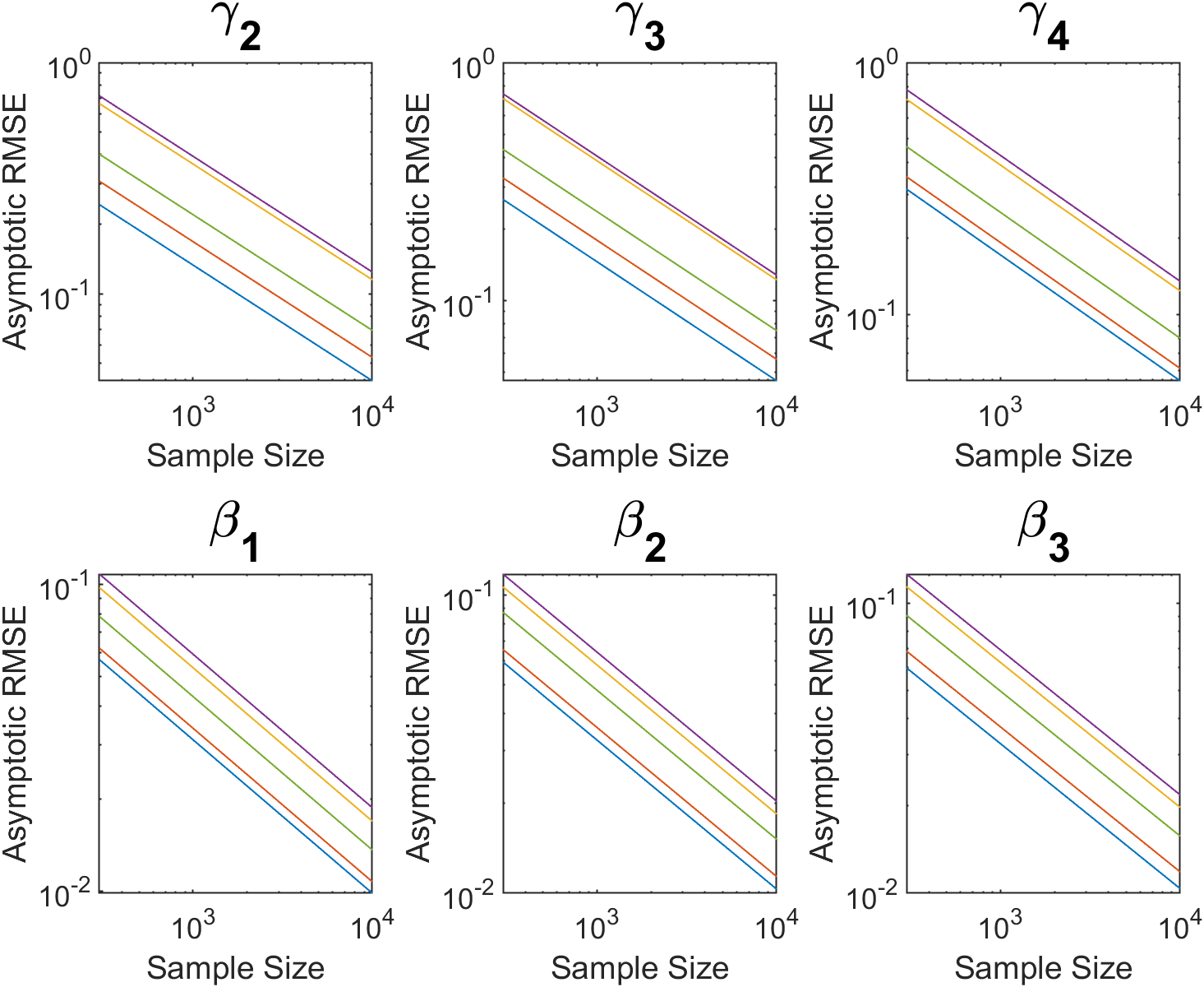
Figure 1: RMSEs Implied by the Asymptotic Distribution for Design 1

The figure shows the root mean squared error as a function of sample size predicted by asymptotic theory for five estimators: The correlated random effects estimator (blue), the estimator that efficiently exploits all the conditional moment conditions (red), efficient GMM based on many unconditional moments (green), efficient GMM based on few unconditional moments (yellow), and inefficient GMM based on few unconditional moments (purple).

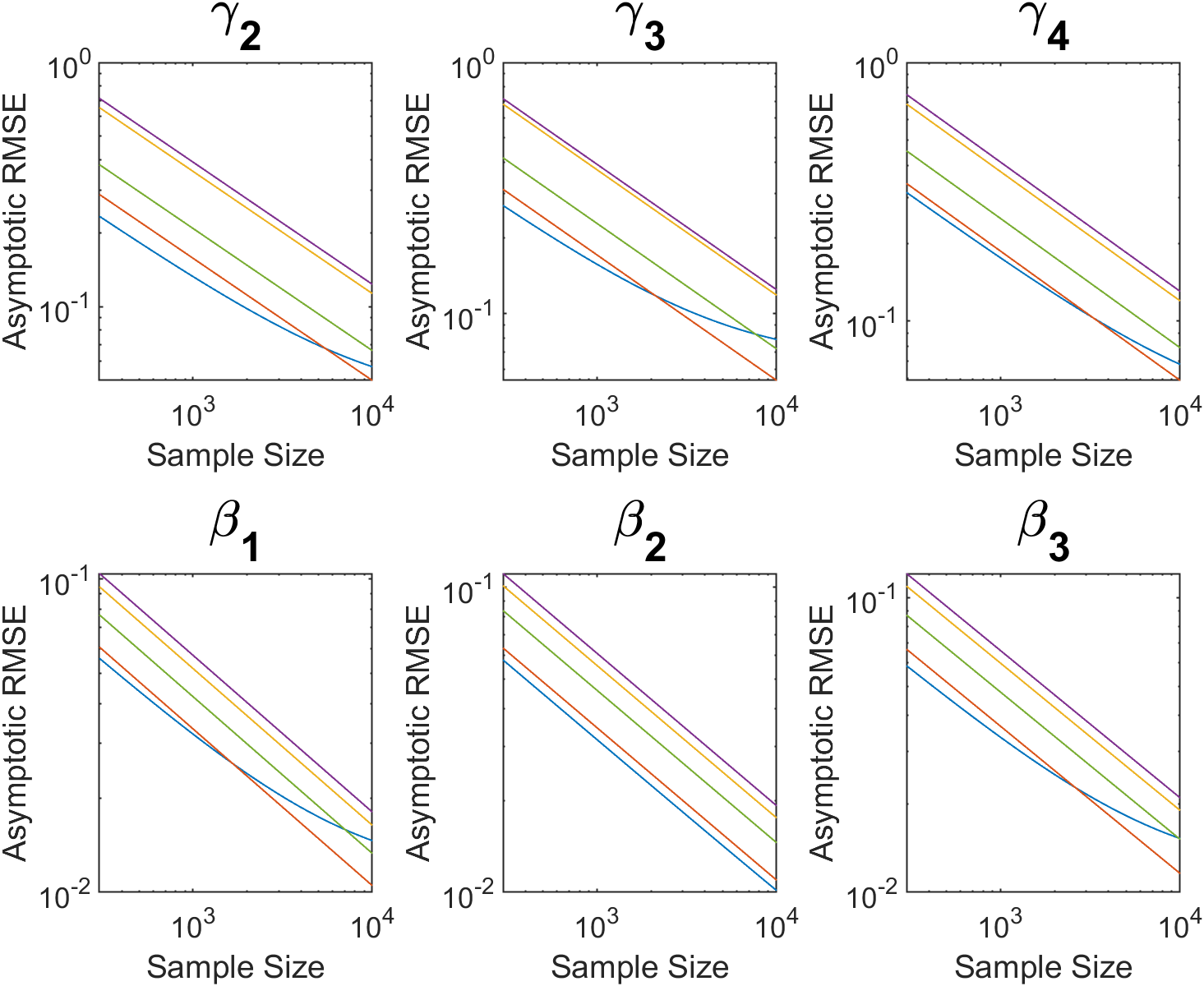
Figure 2: RMSEs Implied by the Asymptotic Distribution for Design 2

The figure shows the root mean squared error as a function of sample size predicted by asymptotic theory for five estimators: The correlated random effects estimator (blue), the estimator that efficiently exploits all the conditional moment conditions (red), efficient GMM based on many unconditional moments (green), efficient GMM based on few unconditional moments (yellow), and inefficient GMM based on few unconditional moments (purple).

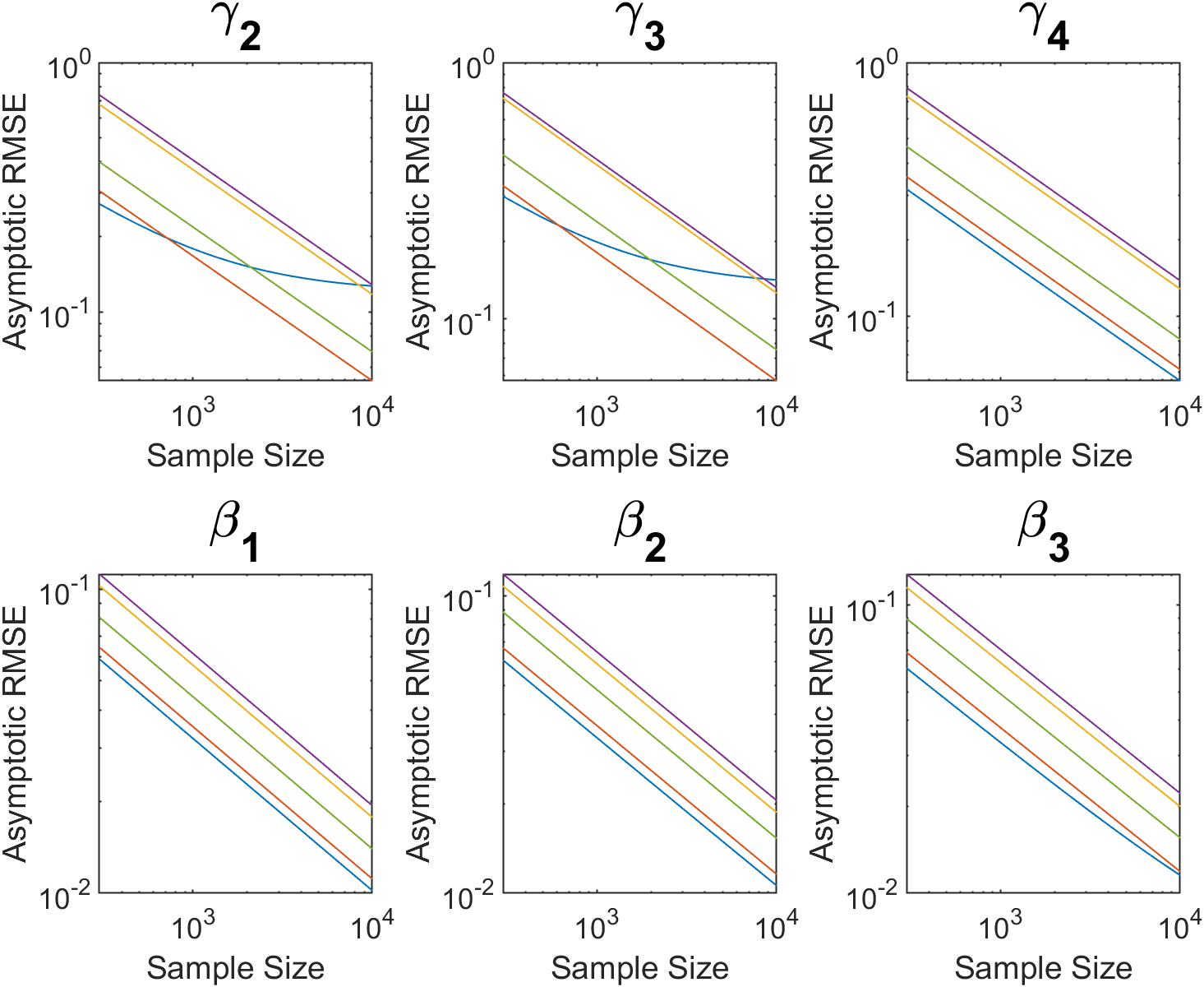
Figure 3: RMSEs Implied by the Asymptotic Distribution for Design 3

The figure shows the root mean squared error as a function of sample size predicted by asymptotic theory for five estimators: The correlated random effects estimator (blue), the estimator that efficiently exploits all the conditional moment conditions (red), efficient GMM based on many unconditional moments (green), efficient GMM based on few unconditional moments (yellow), and inefficient GMM based on few unconditional moments (purple).

Design 1 is a pure random effects specification. Since this is a special case of the correlated random effects estimator, it is not surprising that the correlated random effects estimator is superior to all the GMM estimators in that case. Perhaps surprisingly, the GMM estimator that efficiently combines the conditional moment conditions in (20)-(32) is almost as efficient as the maximum likelihood estimator in this case. Design 2 and 3 demonstrate that the correlated random effects estimator will generally be misspecified and that this will lead to biased estimates. In these designs, the bias is low enough to make the estimator better than the inefficient GMM estimators for moderate sample sizes. Overall, we conclude that the moment conditions proposed in this paper can in principle be very informative about the common parameters in a panel data ordered logit model.

5.3 Empirical illustration

In the section, we illustrate the value of the moment conditions derived in the paper in an empirical example inspired by Contoyannis, Jones, and Rice (2004). The dependent variable is self-reported health status, and we use data from the first four waves of the British Household Panel Survey. This yields a data set with $7233$ individuals observed in 4 time periods including the initial observation (so $T=3$). In the original data set, the dependent variable can take five values. We aggregate these into “Poor or Very Poor” ($8.0\%$ of the observations), “Fair” ($19.1\%$), “Good” ($47.2\%$), and “Excellent” ($25.7\%$). We also consider specifications where the first two are merged into one outcome.

We use two sets of explanatory variables. In the first, we use age and age-squared (measured as $Age/10$ and $(Age-45)^{2}/{100}$, respectively, where $Age$ is measured in years). In the second, we also include log-income. The results are presented in Table 3, which also presents the estimates from a correlated random effects specification. We have normalized the $\delta$-coefficient associated with “Good Health” to be 0 and the threshold ($\lambda$) just below “Good Health” to be 0. The most consistent result presented in Table 3 is a concave relationship between age and self-reported age. For all of the specifications, this relationship is decreasing after the age of 30, although the estimated effect is smaller when we estimated the model using correlated random effects.

The point estimates for the effect of income on self-reported health are positive in columns two and four, but neither is statistically significant.

Table 3: Empirical Results

	GMM					Correlated RE
	Four Outcomes		Three Outcomes			Four Outcomes		Three Outcomes
$Age/10$	-1.214	-1.195	-0.980	-1.261		-0.117	-0.117	-0.128	-0.130
	(0.306)	(0.330)	(0.488)	(0.475)		(0.013)	(0.013)	(0.014)	(0.014)
$(Age-45)^{2}/100$	-0.200	-0.157	-0.304	-0.236		-0.017	-0.003	-0.021	-0.008
	(0.074)	(0.090)	(0.108)	(1.411)		(0.006)	(0.006)	(0.007)	(0.007)
log-income		0.045		0.196			0.142		0.174
		(0.056)		(0.117)			(0.036)		(0.040)
$\delta_{1}$	-0.310	-0.283				-1.522	-1.537
	(0.166)	(0.141)				(0.116)	(0.117)
$\delta_{2}$	-0.313	-0.302	-0.535	-0.489		-0.611	-0.617	-0.773	-0.764
	(0.130)	(0.115)	(0.338)	(0.239)		(0.064)	(0.064)	(0.068)	(0.068)
$\delta_{3}$	0.000	0.000	0.000	0.000		0.000	0.000	0.000	0.000
	(0.000)	(0.000)	(0.000)	(0.000)		(0.000)	(0.000)	(0.000)	(0.000)
$\delta_{4}$	-0.180	-0.185	0.127	0.021		0.551	0.565	0.479	0.434
	(0.128)	(0.115)	(0.146)	(0.115)		(0.069)	(0.069)	(0.067)	(0.067)
$\lambda_{1}$	-2.756	-2.774				-2.487	-2.483
	(0.086)	(0.077)				(0.047)	(0.047)
$\lambda_{2}$	0.000	0.000	0.000	0.000		0.000	0.000	0.000	0.000
	(0.000)	(0.000)	(0.000)	(0.000)		(0.000)	(0.000)	(0.000)	(0.000)
$\lambda_{3}$	3.693	3.700	3.395	3.440		3.567	3.558	3.627	3.637
	(0.126)	(0.130)	(0.155)	(0.120)		(0.055)	(0.056)	(0.055)	(0.056)

6 Conclusions

This paper has extended the analysis in Honoré and Weidner (2020) to provide conditional moment conditions for panel data fixed effects versions of the dynamic ordered logit models like the one considered in Muris, Raposo, and Vandoros (2020). The moment conditions are interesting in their own right, and the paper also illustrates the potential for systematically deriving moment conditions for nonlinear panel models. The moment conditions presented here can be used for estimation as well as for testing more parametric specifications of the individual-specific effects in dynamic ordered logits. For point-identification, it is important to investigate whether the moment conditions are uniquely satisfied at the true parameter values. The paper presents conditions under which this is the case. The paper also proposes a practical strategy for turning the derived conditional moment conditions into unconditional moment conditions that can be used for GMM estimation, and it illustrates the use of the resulting estimator in a small Monte Carlo study as well as in an empirical application.

More broadly, this paper contributes to the literature on panel data estimation of nonlinear models with fixed effects. In this context, the main contribution is to illustrate the potential for applying the functional differencing insights of Bonhomme (2012) to logit-type models.

Appendix A Appendix

A.1 Proof of Theorem 1 and 2

We first want to establish Lemma 1 below, which is key to proving the main text theorems. In order to state the lemma, we require some additional notation. Recall that $Q\in\{2,3,\ldots\}$ is the number of values that the observed outcomes $Y_{it}$ can take. Let $\widetilde{Y}_{1},\widetilde{Y}_{3}\in\{0,1\}$, $\widetilde{Y}_{2}\in\{1,2,3\}$, and $W\in\{1,2,\ldots,Q\}$ be random variables, and let $\widetilde{Y}=(\widetilde{Y}_{1},\widetilde{Y}_{2},\widetilde{Y}_{3})$. For the joint distribution of $\widetilde{Y}$ and $W$ we write

$$p(\widetilde{y},w):={\mathrm{P}r}\left(\widetilde{Y}=\widetilde{y}\;\;\&\;\;W=w\right)$$

and we assume that

$$p(\widetilde{y},w) =p_{3}(\widetilde{y}_{3}\,|\,\widetilde{y}_{2},w)\;\,p_{2}(\widetilde{y}_{2}\,|\,w)\;\,f(w\,|\,\widetilde{y}_{1})\;\,p_{1}(\widetilde{y}_{1}),$$ (75)

where $\widetilde{y}=(\widetilde{y}_{1},\widetilde{y}_{2},\widetilde{y}_{3})$, and

$$p_{1}(\widetilde{y}_{1}) :={\mathrm{P}r}\left(\widetilde{Y}_{1}=\widetilde{y}_{1}\right),$$

$$f(w\,|\,\widetilde{y}_{1}) :=\Pr\left(W=w\,\Big{|}\,\widetilde{Y}_{1}=\widetilde{y}_{1}\right),$$

$$p_{2}(\widetilde{y}_{2}\,|\,w) :={\mathrm{P}r}\left(\widetilde{Y}_{2}=\widetilde{y}_{2}\,\Big{|}\,W=w\right),$$

$$p_{3}(\widetilde{y}_{3}\,|\,\widetilde{y}_{2},w) :={\mathrm{P}r}\left(\widetilde{Y}_{3}=\widetilde{y}_{3}\,\Big{|}\,\widetilde{Y}_{2}=\widetilde{y}_{2},\,W=w\right).$$

We do not impose any assumptions on the transition probabilities $f(w\,|\,\widetilde{y}_{1})$, $p_{3}(\widetilde{y}_{3}\,|\,1,w)$, and $p_{3}(\widetilde{y}_{3}\,|\,3,w)$. All the other transition probabilities are assumed to follow an (ordered) logit model:

$$p_{1}(\widetilde{y}_{1}) =\left\{\begin{array}[]{ll}1-\Lambda(\pi_{1})&\text{if $\widetilde{y}_{1}=0$,}\\ \Lambda(\pi_{1})&\text{if $\widetilde{y}_{1}=1$,}\end{array}\right.$$ (78)

$$p_{2}(\widetilde{y}_{2}\,|\,w) =\left\{\begin{array}[]{ll}1-\Lambda[\pi_{2,1}(w)]&\text{if $\widetilde{y}_{2}=1$,}\\ \Lambda[\pi_{2,1}(w)]-\Lambda[\pi_{2,2}(w)]&\text{if $\widetilde{y}_{2}=2$,}\\ \Lambda[\pi_{2,2}(w)]&\text{if $\widetilde{y}_{2}=3$,}\end{array}\right.$$ (82)

$$p_{3}(\widetilde{y}_{3}\,|\,2,\,w) =\left\{\begin{array}[]{ll}1-\Lambda(\pi_{3})&\text{if $\widetilde{y}_{3}=0$,}\\ \Lambda(\pi_{3})&\text{if $\widetilde{y}_{3}=1$,}\end{array}\right.$$ (85)

where $\Lambda(\xi):=[1+\exp(-\xi)]^{-1}$ is the cumulative distribution function of the logistic distribution, $\pi_{1},\pi_{3}\in\mathbb{R}$ are constants, and $\pi_{2,1},\pi_{2,2}\,:\,\{1,2,\ldots,Q\}\rightarrow\mathbb{R}$ are functions such that $\pi_{2,1}(w)\geq\pi_{2,2}(w)$ for all $w\in\{1,2,\ldots,Q\}$. Notice that $p_{3}(\widetilde{y}_{3}\,|\,2,\,w)$ does not depend on $w$. Finally, we define $m:\{0,1\}\times\{1,2,3\}\times\{0,1\}\times\{1,2,\ldots,Q\}\rightarrow\mathbb{R}$ by

$$m(\widetilde{y},w) :=\left\{\begin{array}[]{ll}\exp\left(\pi_{1}-\pi_{3}\right)\frac{\displaystyle\exp[\pi_{3}-\pi_{2,2}(w)]-1}{\displaystyle\exp\left[\pi_{2,1}(w)-\pi_{2,2}(w)\right]-1}&\text{if }\widetilde{y}_{1}=0,\,\widetilde{y}_{2}=2,\,\widetilde{y}_{3}=0,\\[10.0pt] \exp\left(\pi_{1}-\pi_{3}\right)\frac{\displaystyle 1-\exp[\pi_{2,2}(w)-\pi_{3}]}{\displaystyle 1-\exp\left[\pi_{2,2}(w)-\pi_{2,1}(w)\right]}&\text{if }\widetilde{y}_{1}=0,\,\widetilde{y}_{2}=2,\,\widetilde{y}_{3}=1,\\[10.0pt] \exp\left(\pi_{1}-\pi_{3}\right)&\text{if }\widetilde{y}_{1}=0,\,\widetilde{y}_{2}=3,\\[10.0pt] -1&\text{if }\widetilde{y}_{1}=1,\,\widetilde{y}_{2}=1,\\[10.0pt] -\frac{\displaystyle 1-\exp[\pi_{3}-\pi_{2,1}(w)]}{\displaystyle 1-\exp\left[\pi_{2,2}(w)-\pi_{2,1}(w)\right]}&\text{if }\widetilde{y}_{1}=1,\,\widetilde{y}_{2}=2,\,\widetilde{y}_{3}=0,\\[10.0pt] -\frac{\displaystyle\exp[\pi_{2,1}(w)-\pi_{3}]-1}{\displaystyle\exp\left[\pi_{2,1}(w)-\pi_{2,2}(w)\right]-1}&\text{if }\widetilde{y}_{1}=1,\,\widetilde{y}_{2}=2,\,\widetilde{y}_{3}=1,\\[10.0pt] 0&\text{otherwise}.\end{array}\right.$$ (93)

Lemma 1

Let $\pi_{1},\pi_{3}\in\mathbb{R}$, and $\pi_{2,1},\pi_{2,2}\,:\,\{1,2,\ldots,Q\}\rightarrow\mathbb{R}$ be such that $\pi_{2,1}(w)\geq\pi_{2,2}(w)$, for all $w\in\{1,2,\ldots,Q\}$. Let the random variables $\widetilde{Y}\in\{0,1\}\times\{1,2,3\}\times\{0,1\}$ and $W\in\{1,2,\ldots,Q\}$ be such that their distributions satisfy (75) and (85), and let $m:\{0,1\}\times\{1,2,3\}\times\{0,1\}\times\{1,2,\ldots,Q\}\rightarrow\mathbb{R}$ be defined by (93). Then we have

$$\mathbb{E}\left[m(\widetilde{Y},W)\right]=0.$$

Proof. Define

$$g(\widetilde{y}_{1},w) :=\mathbb{E}\left[m(\widetilde{Y},W)\,\Big{|}\,\widetilde{Y}_{1}=\widetilde{y}_{1},\,W=w\right]$$

$$=\sum_{\widetilde{y}_{2}\in\{1,2,3\}}\,\sum_{\widetilde{y}_{3}\in\{0,1\}}\,m(\widetilde{y},w)\;\,p_{3}(\widetilde{y}_{3}\,|\,\widetilde{y}_{2},w)\;\,p_{2}(\widetilde{y}_{2}\,|\,w),$$

where $\widetilde{y}=(\widetilde{y}_{1},\widetilde{y}_{2},\widetilde{y}_{3})$. Using the expressions for $p_{2}(\widetilde{y}_{2}\,|\,w)$, $p_{3}(\widetilde{y}_{3}\,|\,\widetilde{y}_{2},w)$, and $m(\widetilde{y},w)$ in (85) and (93) one finds that for $\widetilde{y}_{1}=1$ we have

$$g(1,w) =-\left\{1-\Lambda[\pi_{2,1}(w)]\right\}-\left\{\Lambda[\pi_{2,1}(w)]-\Lambda[\pi_{2,2}(w)]\right\}\times$$

$$\qquad\qquad\times\underbrace{\left(\frac{\left[1-\Lambda(\pi_{3})\right]\left\{1-\exp[\pi_{3}-\pi_{2,1}(w)]\right\}}{1-\exp\left[\pi_{2,2}(w)-\pi_{2,1}(w)\right]}+\frac{\Lambda(\pi_{3})\left\{\exp[\pi_{2,1}(w)-\pi_{3}]-1\right\}}{\exp\left[\pi_{2,1}(w)-\pi_{2,2}(w)\right]-1}\right)}_{\displaystyle=\frac{\Lambda[\pi_{2,1}(w)]-\Lambda(\pi_{3})}{\Lambda[\pi_{2,1}(w)]-\Lambda[\pi_{2,2}(w)]}}$$

$$=-\left[1-\Lambda(\pi_{3})\right],$$ (94)

and analogously one calculates for $\widetilde{y}_{1}=0$ that

$$g(0,w) =\exp\left(\pi_{1}-\pi_{3}\right)\Lambda(\pi_{3}).$$ (95)

Notice that $g(\widetilde{y}_{1},w)$ therefore does not depend on $w$, so we can simply write $g(\widetilde{y}_{1}):=g(\widetilde{y}_{1},w)$ in the following. Using (94), (95), and the expression for $p_{1}(\widetilde{y}_{1})$ in (85) we obtain that

$$\sum_{\widetilde{y}_{1}\in\{0,1\}}g(\widetilde{y}_{1})\,p_{1}(\widetilde{y}_{1})=0.$$

Together with $\sum_{w\in\{1,\ldots,Q\}}f(w\,|\,\widetilde{y}_{1})=1$, this gives

$$\mathbb{E}\left[m(\widetilde{Y},W)\right] =\sum_{\widetilde{y}_{1}\in\{0,1\}}\,\sum_{w\in\{1,\ldots,Q\}}\,\sum_{\widetilde{y}_{2}\in\{1,2,3\}}\,\sum_{\widetilde{y}_{3}\in\{0,1\}}\,m(\widetilde{y},w)\,p(\widetilde{y},w)$$

$$=\sum_{\widetilde{y}_{1}\in\{0,1\}}\,\sum_{w\in\{1,\ldots,Q\}}g(\widetilde{y}_{1})\,f(w\,|\,\widetilde{y}_{1})\;p_{1}(\widetilde{y}_{1})$$

$$=\sum_{\widetilde{y}_{1}\in\{0,1\}}\,g(\widetilde{y}_{1})\underbrace{\left[\sum_{w\in\{1,\ldots,Q\}}f(w\,|\,\widetilde{y}_{1})\right]}_{=1}p_{1}(\widetilde{y}_{1})$$

$$=\sum_{\widetilde{y}_{1}\in\{0,1\}}g(\widetilde{y}_{1})\,p_{1}(\widetilde{y}_{1})=0,$$

which is what we wanted to show.    

The following lemma is similar to Lemma 1 above, but the random variables $\widetilde{Y}_{1},\widetilde{Y}_{2},\widetilde{Y}_{3}$ and their distributional assumptions are now different, and the lemma should be understood independently from any notation established above.

Lemma 2

Let $\widetilde{Y}_{1},\widetilde{Y}_{2},\widetilde{Y}_{3}\in\{0,1\}$ and $W,V\in\{1,\ldots,Q\}$ be random variables such that the joint distribution of $\widetilde{Y}=(\widetilde{Y}_{1},\widetilde{Y}_{2},\widetilde{Y}_{3})$, $W$, and $V$ satisfies

$${\mathrm{P}r}\left(\widetilde{Y}=\widetilde{y}\;\;\&\;\;W=w\;\;\&\;\;V=v\right) =p_{3}(\widetilde{y}_{3}\,|\,v)\;\,g(v\,|\,\widetilde{y}_{2},w)\;\,p_{2}(\widetilde{y}_{2}\,|\,w)\;\,f(w\,|\,\widetilde{y}_{1})\;\,p_{1}(\widetilde{y}_{1}),$$

where $\widetilde{y}=(\widetilde{y}_{1},\widetilde{y}_{2},\widetilde{y}_{3})$, and the functions $p_{3}$, $g$, $p_{2}$, and $f$ are appropriate conditional probabilities, while $p_{1}(\widetilde{y}_{1})$ is the marginal distribution of $\widetilde{Y}_{1}$. For $p_{1}(\widetilde{y}_{1})$, $p_{2}(\widetilde{y}_{2}\,|\,w)$, and $p_{3}(\widetilde{y}_{3}\,|\,v)$ we assume logistic binary choice models:

$$p_{1}(\widetilde{y}_{1}) =\Lambda\left[(2\,\widetilde{y}_{1}-1)\,\pi_{1}\right], p_{2}(\widetilde{y}_{2}\,|\,w) =\Lambda\left[(2\,\widetilde{y}_{2}-1)\,\pi_{2}(w)\right], p_{3}(\widetilde{y}_{3}\,|\,v) =\Lambda\left[(2\,\widetilde{y}_{3}-1)\,\pi_{3}(v)\right],$$

where $\pi_{1}\in\mathbb{R}$ is a constant, and $\pi_{2},\pi_{3}:\,\{1,\ldots,Q\}\rightarrow\mathbb{R}$ are functions. The only assumption that we impose on $f(w\,|\,\widetilde{y}_{1})$ and $g(v\,|\,\widetilde{y}_{2},w)$ is that $g(v\,|\,1,w)=g(v\,|\,1)$; that is, conditional on $\widetilde{Y}_{2}=1$ the distribution of $V$ is independent of $W$. Furthermore, let $m:\{0,1\}^{3}\times\{1,\ldots,Q\}^{2}\rightarrow\mathbb{R}$ be given by

$$m(\widetilde{y},w,v) :=\left\{\begin{array}[]{ll}\exp\left[\pi_{1}-\pi_{2}(w)\right]&\text{if }\widetilde{y}=(0,1,0),\\ \exp\left[\pi_{1}-\pi_{3}(v)\right]&\text{if }\widetilde{y}=(0,1,1),\\ -1&\text{if }(\widetilde{y}_{1},\widetilde{y}_{2})=(1,0),\\ \exp\left[\pi_{3}(v)-\pi_{2}(w)\right]-1&\text{if }\widetilde{y}=(1,1,0),\\ 0&\text{otherwise}.\end{array}\right.$$

We then have

$$\mathbb{E}\left[m(\widetilde{Y},W,V)\right]=0.$$

Proof. This lemma is a restatement of Lemma 6 in the 2021 arXiv version of Honoré and Weidner (2020), and the proof can be found there.    

Using Lemma 1 and 2, we are now ready to prove the two main text theorems.

Proof of Theorem 1. We consider the three cases $q_{2}\in\{2,\ldots,Q-1\}$, $q_{2}=Q$, and $q_{2}=1$ separately.

Case $q_{2}\in\{2,\ldots,Q-1\}$:   In this case, we define

$$W :=Y_{1}, \widetilde{Y}_{1} :=\mathbbm{1}\left\{Y_{1}>q_{1}\right\}, \widetilde{Y}_{3} :=\mathbbm{1}\left\{Y_{3}>q_{3}\right\}, \widetilde{Y}_{2} :=\left\{\begin{array}[]{ll}1&\text{if }Y_{2}<q_{2},\\ 2&\text{if }Y_{2}=q_{2},\\ 3&\text{if }Y_{2}>q_{2}.\end{array}\right.$$

Our ordered logit model in (8) then implies that the joint distribution of $\widetilde{Y}=(\widetilde{Y}_{1},\widetilde{Y}_{2},\widetilde{Y}_{3})$ and $W$ conditional on $A=\alpha$, $Y_{0}=y_{0}$, $X=(x_{1},x_{2},x_{3})$, and $\theta=\theta^{0}$ satisfies (75) and (85), as long as we choose

$$f(y_{1}\,|\,1) ={\mathrm{P}r}\left(Y_{1}=y_{1}\,\big{|}\,Y_{1}>q_{1},\,Y_{0}=y_{0},\,X=x,\,A=\alpha\right),$$

$$f(y_{1}\,|\,0) ={\mathrm{P}r}\left(Y_{1}=y_{1}\,\big{|}\,Y_{1}\leq q_{1},\,Y_{0}=y_{0},\,X=x,\,A=\alpha\right),$$

$$p_{3}(\widetilde{y}_{3}\,|\,1,\,y_{1}) =\left\{\begin{array}[]{ll}{\mathrm{P}r}\left(Y_{3}\leq q_{3}\,\big{|}\,Y_{2}<q_{2},\,Y_{1}=y_{1},\,Y_{0}=y_{0},\,X=x,\,A=\alpha\right)&\text{if $\widetilde{y}_{3}=0$,}\\ {\mathrm{P}r}\left(Y_{3}>q_{3}\,\big{|}\,Y_{2}<q_{2},\,Y_{1}=y_{1},\,Y_{0}=y_{0},\,X=x,\,A=\alpha\right)&\text{if $\widetilde{y}_{3}=1$,}\end{array}\right.$$

$$p_{3}(\widetilde{y}_{3}\,|\,3,\,y_{1}) =\left\{\begin{array}[]{ll}{\mathrm{P}r}\left(Y_{3}\leq q_{3}\,\big{|}\,Y_{2}>q_{2},\,Y_{1}=y_{1},\,Y_{0}=y_{0},\,X=x,\,A=\alpha\right)&\text{if $\widetilde{y}_{3}=0$,}\\ {\mathrm{P}r}\left(Y_{3}>q_{3}\,\big{|}\,Y_{2}>q_{2},\,Y_{1}=y_{1},\,Y_{0}=y_{0},\,X=x,\,A=\alpha\right)&\text{if $\widetilde{y}_{3}=1$,}\end{array}\right.$$

and

$$\pi_{1} =\alpha+z(y_{0},x_{1},\theta^{0})-\lambda_{q_{1}}=\alpha+x^{\prime}_{1}\,\beta^{0}+\gamma^{0}_{y_{0}}-\lambda_{q_{1}},$$

$$\pi_{2,1}(y_{1}) =\alpha+z(y_{1},x_{2},\theta^{0})-\lambda_{q_{2}-1}=\alpha+x^{\prime}_{2}\,\beta^{0}+\gamma^{0}_{y_{1}}-\lambda_{q_{2}-1},$$

$$\pi_{2,2}(y_{1}) =\alpha+z(y_{1},x_{2},\theta^{0})-\lambda_{q_{2}}=\alpha+x^{\prime}_{2}\,\beta^{0}+\gamma^{0}_{y_{1}}-\lambda_{q_{2}},$$

$$\pi_{3} =\alpha+z(q_{2},x_{3},\theta^{0})-\lambda_{q_{3}}=\alpha+x^{\prime}_{3}\,\beta^{0}+\gamma^{0}_{q_{2}}-\lambda_{q_{3}},$$

where $w=y_{1}$, and $z(y_{t-1},x_{t},\theta)$ is defined in (7). Plugging those expressions for $\pi_{1}$, $\pi_{2,1}(w)$, $\pi_{2,2}(w)$ and $\pi_{3}$ into the moment function $m(\widetilde{y},w)$ in (93), we find that this moment function exactly coincides with $m_{y_{0},q_{1},q_{2},q_{3}}(y,x,\theta^{0})$ in equation (20) of the main text. Thus, by applying Lemma 1 to the distribution of $Y$ conditional on $A=\alpha$, $Y_{0}=y_{0}$, and $X=x$ (the lemma does not feature those conditioning variables, which is why we are applying the lemma to the conditional distribution), we obtain

$$\mathbb{E}\left[m_{y_{0},q_{1},q_{2},q_{3}}(Y,X,\theta^{0})\,\big{|}\,Y_{0}=y_{0},\,X=x,\,A=\alpha\right] =0,$$

which concludes the proof for the case $q_{2}\in\{2,\ldots,Q-1\}$.

Case $q_{2}=Q$:   In this case, we choose

$$W :=Y_{1}, V :=Y_{2}, \widetilde{Y}_{1} :=\mathbbm{1}\left\{Y_{1}>q_{1}\right\}, \widetilde{Y}_{2} :=\mathbbm{1}\left\{Y_{2}=Q\right\}, \widetilde{Y}_{3} :=\mathbbm{1}\left\{Y_{3}>q_{3}\right\}.$$

Our ordered logit model in (8) then implies that the joint distribution of $\widetilde{Y}=(\widetilde{Y}_{1},\widetilde{Y}_{2},\widetilde{Y}_{3})$, $W$, and $V$ conditional on $A=\alpha$, $Y_{0}=y_{0}$, $X=(x_{1},x_{2},x_{3})$, and $\theta=\theta^{0}$ satisfies the assumptions of Lemma 2, as long as we choose

$$f(y_{1}\,|\,1) ={\mathrm{P}r}\left(Y_{1}=y_{1}\,\big{|}\,Y_{1}>q_{1},\,Y_{0}=y_{0},\,X=x,\,A=\alpha\right),$$

$$f(y_{1}\,|\,0) ={\mathrm{P}r}\left(Y_{1}=y_{1}\,\big{|}\,Y_{1}\leq q_{1},\,Y_{0}=y_{0},\,X=x,\,A=\alpha\right),$$

$$g(y_{2}\,|\,1) =\mathbbm{1}\left\{y_{2}=Q\right\},$$

$$g(y_{2}\,|\,0,y_{1}) ={\mathrm{P}r}\left(Y_{2}=y_{2}\,\big{|}\,Y_{2}<Q,\,Y_{1}=y_{1},\,X=x,\,A=\alpha\right),$$

and

$$\pi_{1} =\alpha+z(y_{0},x_{1},\theta^{0})-\lambda_{q_{1}}=\alpha+x^{\prime}_{1}\,\beta^{0}+\gamma^{0}_{y_{0}}-\lambda_{q_{1}},$$

$$\pi_{2}(y_{1}) =\alpha+z(y_{1},x_{2},\theta^{0})-\lambda_{Q-1}=\alpha+x^{\prime}_{2}\,\beta^{0}+\gamma^{0}_{y_{1}}-\lambda_{Q-1},$$

$$\pi_{3}(y_{2}) =\alpha+z(y_{2},x_{3},\theta^{0})-\lambda_{q_{3}}=\alpha+x^{\prime}_{3}\,\beta^{0}+\gamma^{0}_{y_{2}}-\lambda_{q_{3}},$$

where $w=y_{1}$ and $v=y_{2}$, and $z(y_{t-1},x_{t},\theta)$ is defined in (7). Plugging those expressions for $\pi_{1}$, $\pi_{2}(y_{1})$, and $\pi_{3}(y_{2})$ into the moment function $m(\widetilde{y},w,v)$ in Lemma 2, we find that this moment function exactly coincides with $m_{y_{0},q_{1},Q,q_{3}}(y,x,\theta^{0})$ in equation (32) of the main text. Thus, by applying Lemma 2 to the distribution of $Y$ conditional on $A=\alpha$, $Y_{0}=y_{0}$, and $X=x$ (the lemma does not feature those conditioning variables, which is why we are applying the lemma to the conditional distribution), we obtain

$$\mathbb{E}\left[m_{y_{0},q_{1},Q,q_{3}}(Y,X,\theta^{0})\,\big{|}\,Y_{0}=y_{0},\,X=x,\,A=\alpha\right] =0,$$

which concludes the proof for the case $q_{2}=Q$.

Case $q_{2}=1$:   The result for this case follows from the result for $q_{2}=Q$ by applying the transformation $Y_{t}\mapsto Q+1-Y_{t}$, $\lambda_{q}\mapsto-\lambda_{Q-q}$, $\beta\mapsto-\beta$, $\gamma_{q}\mapsto-\gamma_{Q+1-Y_{t}}$, $A_{i}\mapsto-A_{i}$. This transformation leaves the model probabilities in (9) unchanged but transforms the moment function in (32) into the one in (26), implying that this is also a valid moment function.    

Proof of Theorem 2. As was the case in the proof of Theorem 1, we consider the three cases $q_{2}\in\{2,\ldots,Q-1\}$, $q_{2}=Q$, and $q_{2}=1$ separately.

Case $q_{2}\in\{2,\ldots,Q-1\}$:   In this case, we define

$$W :=Y_{s-1}, \widetilde{Y}_{1} :=\mathbbm{1}\left\{Y_{t}>q_{1}\right\}, \widetilde{Y}_{3} :=\mathbbm{1}\left\{Y_{s+1}>q_{3}\right\}, \widetilde{Y}_{2} :=\left\{\begin{array}[]{ll}1&\text{if }Y_{s}<q_{2},\\ 2&\text{if }Y_{s}=q_{2},\\ 3&\text{if }Y_{s}>q_{2}.\end{array}\right.$$

Let $Y^{t-1}=(Y_{t-1},Y_{t-2},\ldots,Y_{0})$. Our ordered logit model in (8) then implies that the joint distribution of $\widetilde{Y}=(\widetilde{Y}_{1},\widetilde{Y}_{2},\widetilde{Y}_{3})$ and $W$ conditional on $A=\alpha$, $Y^{t-1}=y^{t-1}$, $X=(x_{1},x_{2},x_{3})$, and $\theta=\theta^{0}$ satisfies (75) and (85), as long as we choose

$$f(y_{1}\,|\,1) ={\mathrm{P}r}\left(Y_{t}=y_{1}\,\big{|}\,Y_{t}>q_{1},\,Y^{t-1}=y^{t-1},\,X=x,\,A=\alpha\right),$$

$$f(y_{1}\,|\,0) ={\mathrm{P}r}\left(Y_{t}=y_{1}\,\big{|}\,Y_{t}\leq q_{1},\,Y^{t-1}=y^{t-1},\,X=x,\,A=\alpha\right),$$

$$p_{3}(\widetilde{y}_{3}\,|\,1,\,y_{s-1}) =\left\{\begin{array}[]{ll}{\mathrm{P}r}\left(Y_{s+1}\leq q_{3}\,\big{|}\,Y_{s}<q_{2},\,Y_{s-1}=y_{s-1},\,Y^{t-1}=y^{t-1},\,X=x,\,A=\alpha\right)&\text{if $\widetilde{y}_{3}=0$,}\\ {\mathrm{P}r}\left(Y_{s+1}>q_{3}\,\big{|}\,Y_{s}<q_{2},\,Y_{s-1}=y_{s-1},\,Y^{t-1}=y^{t-1},\,X=x,\,A=\alpha\right)&\text{if $\widetilde{y}_{3}=1$,}\end{array}\right.$$

$$p_{3}(\widetilde{y}_{3}\,|\,3,\,y_{s-1}) =\left\{\begin{array}[]{ll}{\mathrm{P}r}\left(Y_{s+1}\leq q_{3}\,\big{|}\,Y_{s}>q_{2},\,Y_{s-1}=y_{s-1},\,Y^{t-1}=y^{t-1},\,X=x,\,A=\alpha\right)&\text{if $\widetilde{y}_{3}=0$,}\\ {\mathrm{P}r}\left(Y_{s+1}>q_{3}\,\big{|}\,Y_{s}>q_{2},\,Y_{s-1}=y_{s-1},\,Y^{t-1}=y^{t-1},\,X=x,\,A=\alpha\right)&\text{if $\widetilde{y}_{3}=1$,}\end{array}\right.$$

and

$$\pi_{1} =\alpha+z(y_{t-1},x_{t},\theta^{0})-\lambda_{q_{1}}=\alpha+x^{\prime}_{t}\,\beta^{0}+\gamma^{0}_{y_{t-1}}-\lambda_{q_{1}},$$

$$\pi_{2,1}(y_{1}) =\alpha+z(y_{s-1},x_{s},\theta^{0})-\lambda_{q_{2}-1}=\alpha+x^{\prime}_{s}\,\beta^{0}+\gamma^{0}_{y_{s-1}}-\lambda_{q_{2}-1},$$

$$\pi_{2,2}(y_{1}) =\alpha+z(y_{s-1},x_{s},\theta^{0})-\lambda_{q_{2}}=\alpha+x^{\prime}_{s}\,\beta^{0}+\gamma^{0}_{y_{s-1}}-\lambda_{q_{2}},$$

$$\pi_{3} =\alpha+z(q_{s},x_{s+1},\theta^{0})-\lambda_{q_{3}}=\alpha+x^{\prime}_{s+1}\,\beta^{0}+\gamma^{0}_{q_{2}}-\lambda_{q_{3}},$$

where $w=y_{s-1}$, and $z(y_{t-1},x_{t},\theta)$ is defined in (7). Plugging those expressions for $\pi_{1}$, $\pi_{2,1}(w)$, $\pi_{2,2}(w)$ and $\pi_{3}$ into the moment function $m(\widetilde{y},w)$ in (93) we find that this moment function exactly coincides with $m^{(t,s,s+1)}_{y_{0},q_{1},q_{2},q_{3}}(y,x,\theta^{0})$ in equation (40) of the main text. Thus, by applying Lemma 1 to the distribution of $Y$ conditional on $A=\alpha$, $Y^{t-1}=y^{t-1}$, and $X=x$ (the lemma does not feature those conditioning variables, which is why we are applying the lemma to the conditional distribution), we obtain

$$\mathbb{E}\left[m^{(t,s,s+1)}_{y_{0},q_{1},q_{2},q_{3}}(Y,X,\theta^{0})\,\big{|}\,Y^{t-1}=y^{t-1},\,X=x,\,A=\alpha\right] =0.$$

Applying the law of iterated expectations, we thus also find that

$$\mathbb{E}\left[w(Y_{1},\ldots,Y_{t-1})\,m^{(t,s,s+1)}_{y_{0},q_{1},q_{2},q_{3}}(Y,X,\theta^{0})\,\Big{|}\,Y_{0}=y_{0},\,X=x,\,A=\alpha\right] =0,$$

which concludes the proof for the case $q_{2}\in\{2,\ldots,Q-1\}$.

Case $q_{2}=Q$:   In this case, we choose

$$W :=Y_{s-1}, V :=Y_{r-1}, \widetilde{Y}_{t} :=\mathbbm{1}\left\{Y_{1}>q_{1}\right\}, \widetilde{Y}_{s} :=\mathbbm{1}\left\{Y_{2}=Q\right\}, \widetilde{Y}_{r} :=\mathbbm{1}\left\{Y_{3}>q_{3}\right\}.$$

Our ordered logit model in (8) then implies that the joint distribution of $\widetilde{Y}=(\widetilde{Y}_{1},\widetilde{Y}_{2},\widetilde{Y}_{3})$, $W$, and $V$ conditional on $A=\alpha$, $Y^{t-1}=y^{t-1}$, $X=(x_{1},x_{2},x_{3})$, and $\theta=\theta^{0}$ satisfies the assumptions of Lemma 2, as long as we choose

$$f(y_{s-1}\,|\,1) ={\mathrm{P}r}\left(Y_{s-1}=y_{s-1}\,\big{|}\,Y_{t}>q_{1},\,Y^{t-1}=y^{t-1},\,X=x,\,A=\alpha\right),$$

$$f(y_{s-1}\,|\,0) ={\mathrm{P}r}\left(Y_{s-1}=y_{s-1}\,\big{|}\,Y_{t}\leq q_{1},\,Y^{t-1}=y^{t-1},\,X=x,\,A=\alpha\right),$$

$$g(y_{r-1}\,|\,1) =\mathbbm{1}\left\{y_{r-1}=Q\right\},$$

$$g(y_{r-1}\,|\,0,y_{s-1}) ={\mathrm{P}r}\left(Y_{r-1}=y_{r-1}\,\big{|}\,Y_{s}<Q,\,Y_{s-1}=y_{s-1},\,X=x,\,A=\alpha\right),$$

and

$$\pi_{1} =\alpha+z(y_{t-1},x_{t},\theta^{0})-\lambda_{q_{1}}=\alpha+x^{\prime}_{t}\,\beta^{0}+\gamma^{0}_{y_{t-1}}-\lambda_{q_{1}},$$

$$\pi_{2}(y_{s-1}) =\alpha+z(y_{s-1},x_{s},\theta^{0})-\lambda_{Q-1}=\alpha+x^{\prime}_{s}\,\beta^{0}+\gamma^{0}_{y_{s-1}}-\lambda_{Q-1},$$

$$\pi_{3}(y_{r-1}) =\alpha+z(y_{r-1},x_{r},\theta^{0})-\lambda_{q_{3}}=\alpha+x^{\prime}_{r}\,\beta^{0}+\gamma^{0}_{y_{r-1}}-\lambda_{q_{3}},$$

where $w=y_{s-1}$ and $v=y_{r-1}$, and $z(y_{t-1},x_{t},\theta)$ is defined in (7). Plugging those expressions for $\pi_{1}$, $\pi_{2}(y_{s-1})$, and $\pi_{3}(y_{r-1})$ into the moment function $m(\widetilde{y},w,v)$ in Lemma 2 we find that this moment function exactly coincides with $m_{y_{0},q_{1},Q,q_{3}}(y,x,\theta^{0})$ in equation (52) of the main text. Thus, by applying Lemma 2 to the distribution of $Y$ conditional on $A=\alpha$, $Y^{t-1}=y^{t-1}$, and $X=x$ (the lemma does not feature those conditioning variables, which is why we are applying the lemma to the conditional distribution) we obtain

$$\mathbb{E}\left[m^{(t,s,r)}_{y_{0},q_{1},Q,q_{3}}(Y,X,\theta^{0})\,\Big{|}\,Y^{t-1}=y^{t-1},\,X=x,\,A=\alpha\right] =0.$$

Applying the law of iterated expectations, we thus also find that

$$\mathbb{E}\left[w(Y_{1},\ldots,Y_{t-1})\,m^{(t,s,r)}_{y_{0},q_{1},Q,q_{3}}(Y,X,\theta^{0})\,\Big{|}\,Y_{0}=y_{0},\,X=x,\,A=\alpha\right] =0,$$

which concludes the proof for the case $q_{2}=Q$.

Case $q_{2}=1$:   The result for this case again follows from the result for $q_{2}=Q$ by applying the transformation $Y_{t}\mapsto Q+1-Y_{t}$, $\lambda_{q}\mapsto-\lambda_{Q-q}$, $\beta\mapsto-\beta$, $\gamma_{q}\mapsto-\gamma_{Q+1-Y_{t}}$, $A_{i}\mapsto-A_{i}$.    

A.2 Proof of Proposition 1, 2, and 3

The following lemma is useful for the proof of Proposition 1.

Lemma 3

Let $Q\geq 2$. Let $B$ be a $Q\times Q$ matrix for which all non-diagonal elements are positive (i.e. $B_{q,r}>0$ for $q\neq r$). Let $g^{0},g\in(0,\infty)^{Q}$ be two vectors with only positive entries. Assume that $Bg^{0}=0$ and $Bg=0$. Then there exists $\kappa>0$ such that $g=\kappa\,g^{0}$.

Proof. This is a proof by contradiction. Let all assumptions of the lemma be satisfied, and assume that there does not exist a $\kappa>0$ such that $g=\kappa\,g^{0}$. Define the vector $h\in[0,\infty)^{Q}$ and the two sets ${\cal Q}_{+},{\cal Q}_{0}\subset\{1,\ldots,Q\}$ by

$$h :=g^{0}-\left(\min_{q\in\{1,\ldots,Q\}}\frac{g^{0}_{q}}{g_{q}}\right)\,g, {\cal Q}_{+} :=\left\{q\,:\,h_{q}>0\right\}, {\cal Q}_{0} :=\left\{q\,:\,h_{q}=0\right\}.$$

All elements of $h$ are non-negative by construction, and we have $h\neq 0$, because otherwise we would have $g=\kappa\,g^{0}$ for some $\kappa>0$. Therefore, neither ${\cal Q}_{+}$ nor ${\cal Q}_{0}$ are empty sets. Furthermore, since $h$ is a linear combination of $g^{0}$ and $g$, and we have $Bg^{0}=Bg=0$, we also have $Bh=0$. This can equivalently be written as

$$\sum_{r\in{\cal Q}_{+}}\,B_{q,r}\;h_{r}=0,\qquad\text{for all }q\in\{1,\ldots,Q\},$$

where we dropped the indices $r$ from the sum for which we have $h_{r}=0$.

Now, let $q\in{\cal Q}_{0}$. We then have $q\notin{\cal Q}_{+}$, and therefore $B_{q,r}>0$ for all $r\in{\cal Q}_{+}$, according to our assumption on $B$. We have argued that ${\cal Q}_{+}$ is non-empty, and by construction we have $h_{q}>0$ for $q\in{\cal Q}_{+}$. We therefore have

$$\sum_{r\in{\cal Q}_{+}}\,B_{q,r}\;h_{r}>0.$$

The last two displays are the contradiction that we wanted to derive here.    

Proof of Proposition 1. Let $x_{(1)}=(x_{1},x_{1},x_{1})$. For $y_{0},q\in\{1,\ldots,Q\}$ we define

$$B_{y_{0},q}:=\left\{\begin{array}[]{ll}{\mathrm{P}r}\left(y_{1}>1\;\&\;y_{2}=1\;\&\;y_{3}=1\mid Y_{0}=y_{0},\,X=x_{(1)}\right)&\text{if $y_{0}\neq q$ and $q=1$,}\\ {\mathrm{P}r}\left(y_{1}=q\;\&\;y_{2}=1\;\&\;y_{3}>1\mid Y_{0}=y_{0},\,X=x_{(1)}\right)&\text{if $y_{0}\neq q$ and $q>1$,}\\ {\mathrm{P}r}\left(y_{1}>1\;\&\;y_{2}=1\;\&\;y_{3}=1\mid Y_{0}=y_{0},\,X=x_{(1)}\right)\\ \qquad\qquad\qquad-{\mathrm{P}r}\left(y_{1}=1\;\&\;y_{2}>1\mid Y_{0}=y_{0},\,X=x_{(1)}\right)&\text{if $y_{0}=q$ and $q=1$,}\\ {\mathrm{P}r}\left(y_{1}=q\;\&\;y_{2}=1\;\&\;y_{3}>1\mid Y_{0}=y_{0},\,X=x_{(1)}\right)\\ \qquad\qquad\qquad-{\mathrm{P}r}\left(y_{1}=1\;\&\;y_{2}>1\mid Y_{0}=y_{0},\,X=x_{(1)}\right)&\text{if $y_{0}=q$ and $q>1$.}\end{array}\right.$$

Let $B$ be the $Q\times Q$ matrix with entries $B_{y_{0},q}$. Our assumptions guarantee that all the conditional probabilities that enter into the definition of $B_{y_{0},q}$ are non-negative, and we therefore have

$$B_{y_{0},q} >0,\qquad\text{for all $y_{0}\neq q$}.$$ (96)

Applying Theorem 1 we find that the moment function in (60) satisfies

$$\mathbb{E}\left[m_{y_{0}}(y,\gamma^{0})\mid Y_{0}=y_{0},\,X=(x_{1},x_{1},x_{1})\right]=0,\qquad\text{for all $y_{0}\in\{1,\ldots,Q\}$},$$ (97)

where $\gamma^{0}$ is the true parameter that generates the data. In the proposition, we assume that $\gamma\in\mathbb{R}^{Q}$ is an alternative parameter that satisfies the same moment conditions. Let $g^{0}$ and $g$ be the $Q$-vectors with entries $g^{0}_{q}:=\exp\left(\gamma^{0}_{q}\right)>0$ and $g_{q}:=\exp\left(\gamma_{q}\right)$. Using the definition of the matrix $B$ we can rewrite the two systems of $Q$ equations in (97) and (61) as

$$B\,g^{0} =0, B\,g=0.$$ (98)

Since we have (96) and (98) we can apply Lemma 3 to find that there exists $\kappa>0$ such that $g=\kappa\,g^{0}$. Taking logarithms, we thus have $\gamma=\gamma^{0}+c$, where $c=\log(\kappa)$. This is what we wanted to show.    

The following lemma is useful for the proof of Proposition 2.

Lemma 4

Let $K\in\mathbb{N}$. For every $s=(s_{1},\ldots,s_{K-1},+)\in\{-,+\}^{K}$, let $g_{s}:\mathbb{R}^{K}\rightarrow\mathbb{R}$ be a continuous function such that for all $\beta\in\mathbb{R}^{K}$, we have

• $g_{s}(\beta)$ is strictly increasing in $\beta_{K}$.

• For all $m\in\{1,\ldots,K-1\}$: If $s_{m}=+$, then $g_{s}(\beta)$ is strictly increasing in $\beta_{m}$.

• For all $m\in\{1,\ldots,K-1\}$: If $s_{k}=-$, then $g_{s}(\beta)$ is strictly decreasing in $\beta_{m}$.

Then, the system of $2^{K-1}$ equations in $K$ variables

$$g_{s}(\beta)=0\qquad\text{for all $s\in\{-,+\}^{K}$ with $s_{K}=+$,}$$

has at most one solution.

Proof. This is the same as Lemma 2 in Honoré and Weidner (2020), only presented using slightly different notation here.    

Proof of Proposition 2. For $s=(s_{1},\ldots,s_{K-1},+)\in\{-,+\}^{K}$ we define

$$g_{s}(\beta)=\mathbb{E}\left[m_{y_{0},1,1,1}(Y,X,\beta,\gamma_{0})\,\Big{|}\,Y_{0}=y_{0},\;X\in\mathcal{X}_{s}\right],$$ (99)

where $m_{y_{0},1,1,1}(y,x,\beta,\gamma)$ is the moment function in (67). Our assumptions guarantee that the conditioning sets in (99) have positive probability, which, together with the definition of $m_{y_{0},1,1,1}(y,x,\beta,\gamma_{0})$ and $\mathcal{X}_{s}$, guarantee that the functions $g_{s}(\beta)$ satisfy the monotonicity requirements (i), (ii) and (iii) of Lemma 4. Theorem 1 guarantees that

$$g_{s}(\beta^{0})=0,\qquad\text{for all $s\in\{-,+\}^{K}$ with $s_{K}=+$,}$$

where $\beta^{0}$ is the true parameter value that generates the data. Equation (68) in the proposition can equivalently be written as

$$g_{s}(\beta)=0,\qquad\text{for all $s\in\{-,+\}^{K}$ with $s_{K}=+$.}$$

According to Lemma 4, the system of equations in the last two displays can have at most one solution, and we, therefore, must have $\beta=\beta_{0}$.    

Proof of Proposition 3. The definition of $m_{y_{0},q_{1},1,1}(y,x,\beta,\gamma,\lambda)$ in (74) together with the assumptions of the proposition guarantee that $g(\lambda):=\mathbb{E}\left[m_{y_{0},q_{1},1,1}(Y,X,\beta^{0},\gamma^{0},\lambda)\,\Big{|}\,Y_{0}=y_{0}\right]$ is strictly increasing in $\lambda_{q_{1}}-\lambda_{1}$ for all $q_{1}\in\{2,\ldots,Q-1\}$. Theorem 1 guarantees that $g(\lambda^{0})=0$ for the true parameter $\lambda^{0}$ that generates the data. For any $\lambda\in\mathbb{R}^{Q-1}$ that satisfies $g(\lambda)=0$, we therefore must have $\lambda_{q_{1}}-\lambda_{1}=\lambda^{0}_{q_{1}}-\lambda^{0}_{1}$, which implies $\lambda=\lambda^{0}+c$ for $c=\lambda_{1}-\lambda^{0}_{1}$.    

A.3 Lower bound on the number of moment conditions

Dobronyi, Gu, and Kim (2021) point out that it is sometimes possible to easily derive a lower bound on the number of linearly independent valid moment conditions in a given panel data model. The key insight (to be verified below) is that one can write the model probabilities defined in equation (9) as

$$p_{y_{0}}(y,x,\theta,\alpha)=\kappa\left(a\right)\,\sum_{k=1}^{K}a^{k-1}c_{k}\left(y\right),$$ (100)

for some constant $K\in\{1,2,\ldots\}$, some positive function $\kappa$ of $a=\exp\left(\alpha\right)$ that does not depend on $y$, and some functions $c_{k}$ of $y$ that do not depend on $a$. Here, the functions $\kappa$ and $c_{k}$ also depend on $y_{0}$, $x$, $\theta$, but those arguments are dropped to focus more clearly on the dependence on $\alpha$ and $y$. In other words, $y_{0}$, $x$, $\theta$ are simply assumed fixed here. The dependence of all functions and constants on $T$ is also not made explicit (here or anywhere else in the paper).

Once we have shown (100), then a a valid moment function must satisfy

$$\sum_{y\in\mathcal{Y}}m(y)\,\sum_{k=1}^{K}a^{k-1}c_{k}\left(y\right)=0,\qquad\text{for all }a\in\left(0,\infty\right),$$ (101)

which is equivalent to

$$\sum_{y\in\mathcal{Y}}\,m(y)\,c_{k}(y)=0,\qquad\text{for all $k\in\{1,\ldots,K\}$.}$$

These are $K$ linear conditions in $Q^{T}$ unknown parameters $m(y)$. We, therefore, have at least $Q^{T}-K$ linearly independent solutions $m(y)$. In other words, the model must have at least $Q^{T}-K$ linearly independent conditional moment conditions.

What is left to do now is to show that (100) indeed holds for our the dynamic order choice model, for some $K<Q^{T}$. For that purpose, remember that $\Lambda(\varepsilon)=[1+\exp(-\varepsilon)]^{-1}$, and also define $\omega_{t,q}=X_{t}^{\prime}\,\beta-\lambda_{q},$ and

$$a =\exp(\alpha), w_{q} =\exp(\omega_{t,q}), g_{q} =\exp(\gamma_{q}).$$

Also remember that $\lambda_{0}=-\infty$ and $\lambda_{Q}=\infty$, which implies that

$$w_{0} =\infty, w_{Q} =0.$$

According to (9), the probability of observing $Y=y$, conditional on $Y_{0}=y_{0}$, $X=x$, $A=\alpha$, $\theta=\theta_{0}$, is then given by

$$p_{y_{0}}(y,x,\theta,\alpha) =\prod_{t=1}^{T}\left\{\Lambda\Big{[}\omega_{t,(y_{t}-1)}+\gamma_{y_{t-1}}+\alpha\Big{]}-\Lambda\Big{[}\omega_{t,y_{t}}+\gamma_{y_{t-1}}+\alpha\Big{]}\right\}$$

$$=\prod_{t=1}^{T}\left\{\frac{w_{t,(y_{t}-1)}\,g_{y_{t-1}}\,a}{1+w_{t,(y_{t}-1)}\,g_{y_{t-1}}\,a}-\frac{w_{t,y_{t}}\,g_{y_{t-1}}\,a}{1+w_{t,y_{t}}\,g_{y_{t-1}}\,a}\right\}$$

$$=\kappa\left(a\right)\,\widetilde{p}(y,a),$$

where

$$\kappa\left(a\right) =\prod_{q=1}^{Q-1}\,\frac{1}{1+w_{t,q}\,g_{y_{0}}\,a}\,\prod_{t=2}^{T}\prod_{r=1}^{Q}\frac{1}{1+w_{t,q}\,g_{r}\,a},$$

and

$$\widetilde{p}(y,a) =\bigg{\{}\mathbbm{1}\{y_{1}\neq 1\}\,w_{1,(y_{1}-1)}\,g_{y_{0}}\,a\prod_{q\in\{1,\ldots,Q-1\}\setminus\{y_{1}-1\}}\,\left(1+w_{1,q}\,g_{y_{0}}\,a\right)$$

$$\qquad\qquad\qquad\qquad-\mathbbm{1}\{y_{1}=Q\}-\mathbbm{1}\{y_{1}\neq Q\}\,w_{1,y_{1}}\,g_{y_{0}}\,a\,\prod_{q\in\{1,\ldots,Q-1\}\setminus\{y_{1}\}}\,\left(1+w_{1,q}\,g_{y_{0}}\,a\right)\bigg{\}}$$

$$\quad\times\prod_{t=2}^{T}\bigg{\{}\mathbbm{1}\{y_{t}\neq 1\}\,w_{t,(y_{t}-1)}\,g_{y_{t-1}}\,a\prod_{(q,r)\in\{1,\ldots,Q-1\}\times\{1,\ldots,Q\}\setminus\{(y_{t}-1,y_{t-1}\}}\,\left(1+w_{t,q}\,g_{r}\,a\right)$$

$$\quad-\mathbbm{1}\{y_{t}=Q\}-\mathbbm{1}\{y_{t}\neq Q\}\,w_{t,y_{t}}\,g_{y_{t-1}}\,a\,\prod_{(q,r)\in\{1,\ldots,Q-1\}\times\{1,\ldots,Q\}\setminus\{(y_{t},y_{t-1}\}}\,\left(1+w_{t,q}\,g_{y_{r}}\,a\right)\bigg{\}}.$$

Here, $\kappa(a)$ does not depend on $y$, and $\widetilde{p}(y,a)$ is a polynomial in $a$ of order

$$K-1=(Q-1)+(T-1)Q(Q-1).$$

This implies that a lower bound on the number of linearly independent valid moment conditions in this model is given by

$$Q^{T}-K =Q^{T}-Q-(T-1)Q(Q-1)$$

$$=Q^{T}-(T-1)Q^{2}+(T-2)Q,$$

which is exactly the number of linearly independent valid moment conditions we found in the main text.

A.4 Computational details

From an estimation point of view, it is natural to estimate $\left(\beta,\gamma,\lambda\right)$ by applying generalized methods of moments to a finite-dimensional vector of unconditional moment conditions derived from (20), (26), and (32). There are at least two problems with this. The first is that, as discussed in Section 3 above, one needs to worry about whether the moment conditions actually identify the parameters of interest. The second problem is that even if one ignores the issue of identification, there are many ways to form a finite set of unconditional moment conditions from the expressions in (20), (26), and (32). Of course, it is in principle known how to most efficiently turn a set of conditional moment conditions into a set of moment conditions of the same dimensionality as the parameter to be estimated. See, for example, the discussion in Newey and McFadden (1994). Specifically, with a conditional moment condition $\mathbb{E}\left[\left.m\left(Y,X,\theta\right)\right|X\right]=0$ when $\theta$ takes its true value, $\theta_{0}$, the optimal unconditional moment function is $A\left(X\right)m\left(Y,X,\theta\right)$, where $A\left(X\right)=\mathbb{E}\left[\left.\nabla_{\theta}m\left(Y,X,\theta_{0}\right)\right|X\right]^{\prime}V\left[\left.m\left(Y,X,\theta_{0}\right)\right|X\right]$. Unfortunately, the construction of estimators of these efficient moments depends heavily on the distribution of $Y$ given $X$. In the fixed effects context, this will depend on the distribution of the fixed effects conditional on all the explanatory variables. This prevents a simple two-step procedure for efficiently estimating $\left(\beta,\gamma,\lambda\right)$ from the conditional moment conditions. To turn the conditional moment conditions in Theorem 1 into an estimator, we therefore use a slightly different approach.

We first estimate $\left(\beta,\gamma,\lambda\right)$ by GMM using a fairly arbitrary set of moment conditions. In practice, we consider the moments constructed by interacting each of the conditional moments in Theorem 1 with each element of $\left(1,X_{i1}-X_{i2},X_{i1}-X_{i3},X_{i2}-X_{i3}\right)$. We then first calculate the GMM estimator based on the following simple diagonal weight matrix. We set $\beta$ and $\gamma$ to vectors of 0’s and estimate $\lambda$ by maximum likelihood estimation under the assumption that there is no individual-specific heterogeneity. We then calculate the empirical variance of each moment and use the inverse of those as the diagonal elements of the weight matrix (except when the sample variance is 0, in which case the weight is set to 0). This yields an initial GMM estimator of $\left(\beta,\gamma,\lambda\right)$. We use this to calculate the empirical variance of each moment. The inverse of those are then used as diagonal elements of a diagonal weight matrix, which is in turn used to form a second GMM estimator. Finally, we use this estimator of $\left(\beta,\gamma,\lambda\right)$ to calculate the sample covariance matrix of the moments. The inverse of this is used as the weight matrix for a final GMM estimator, except that we inflate the diagonal elements of the covariance matrix by 10% before inverting it. This is done to overcome numerical problems associated with collinear moments.

We next estimate a flexible reduced form model for the distribution of $Y$ given $X$. One may think of this as a nonparametric sieve estimator in which case our approach will be an attempt to construct the efficient estimator. Alternatively, one can acknowledge that the model for $Y$ given $X$ is most likely incorrect, in which case the approach can be interpreted as an attempt to construct unconditional moments that are close to the efficient ones. In practice, we estimate the reduced form model for the distribution of $Y$ given $X$ using a period-by-period ordered logit model where the explanatory variables are all observed lagged $Y$, the contemporaneous $X$, and the average $X$ over all time periods. We then use this reduced form for the distribution of $Y$ given $X$ along with the last GMM estimator in the previous paragraph to construct an estimate of $A\left(X\right)$.

References

- (1)
- Aguirregabiria and Carro (2021) Aguirregabiria, V., and J. M. Carro (2021): “Identification of Average Marginal Effects in Fixed Effects Dynamic Discrete Choice Models,” unpublished, pp. 1–31.
- Aguirregabiria, Gu, and Luo (2021) Aguirregabiria, V., J. Gu, and Y. Luo (2021): “Sufficient Statistics for Unobserved Heterogeneity in Structural Dynamic Logit Models,” Journal of Econometrics, 223(2), 280–311.
- Albarran, Carrasco, and Carro (2019) Albarran, P., R. Carrasco, and J. M. Carro (2019): “Estimation of Dynamic Nonlinear Random Effects Models with Unbalanced Panels,” Oxford Bulletin of Economics and Statistics, 81(6), 1424–1441.
- Arellano (2003) Arellano, M. (2003): “Discrete choices with panel data,” Investigaciones económicas, 27(3), 423–458.
- Arellano and Bond (1991) Arellano, M., and S. Bond (1991): “Some Tests of Specification for Panel Data: Monte Carlo Evidence and an Application to Employment Equations,” The Review of Economic Studies, 58(2), 277.
- Arellano and Bonhomme (2011) Arellano, M., and S. Bonhomme (2011): “Nonlinear Panel Data Analysis,” Annual Review of Economics, 3(1), 395–424.
- Aristodemou (2021) Aristodemou, E. (2021): “Semiparametric Identification in Panel Data Discrete Response Models,” Journal of Econometrics, 220(2), 253–271.
- Baetschmann, Staub, and Winkelmann (2015) Baetschmann, G., K. E. Staub, and R. Winkelmann (2015): “Consistent estimation of the fixed effects ordered logit model,” Journal of the Royal Statistical Society A, 178(3), 685–703.
- Blundell and Bond (1998) Blundell, R., and S. Bond (1998): “Initial conditions and moment restrictions in dynamic panel data models,” Journal of Econometrics, 87(1), 115–143.
- Bonhomme (2012) Bonhomme, S. (2012): “Functional differencing,” Econometrica, 80(4), 1337–1385.
- Botosaru, Muris, and Pendakur (2023) Botosaru, I., C. Muris, and K. Pendakur (2023): “Identification of Time-Varying Transformation Models with Fixed Effects, with an Application to Unobserved Heterogeneity in Resource Shares,” Journal of Econometrics, 232(2), 576–597.
- Carro and Traferri (2014) Carro, J. M., and A. Traferri (2014): “State Dependence and Heterogeneity in Health Using a Bias-Corrected Fixed-Effects Estimator,” Journal of Applied Econometrics, 29(2), 181–207.
- Chamberlain (1980) Chamberlain, G. (1980): “Analysis of Covariance with Qualitative Data,” The Review of Economic Studies, 47(1), 225–238.
- Chamberlain (1985) (1985): “Heterogeneity, Omitted Variable Bias, and Duration Dependence,” in Longitudinal Analysis of Labor Market Data, ed. by J. J. Heckman, and B. Singer, no. 10 in Econometric Society Monographs series, pp. 3–38. Cambridge University Press, Cambridge, New York and Sydney.
- Contoyannis, Jones, and Rice (2004) Contoyannis, P., A. M. Jones, and N. Rice (2004): “The dynamics of health in the British Household Panel Survey,” Journal of Applied Econometrics, 19(4), 473–503.
- Das and van Soest (1999) Das, M., and A. van Soest (1999): “A panel data model for subjective information on household income growth,” Journal of Economic Behavior & Organization, 40(4), 409–426.
- Davezies, D’Haultfoeuille, and Mugnier (2022) Davezies, L., X. D’Haultfoeuille, and M. Mugnier (2022): “Fixed Effects Binary Choice Models with Three or More Periods,” Quantitative Economics (forthcoming).