MD-split+: Practical Local Conformal Inference in High Dimensions

Abstract

Quantifying uncertainty in model predictions is a common goal for practitioners seeking more than just point predictions. One tool for uncertainty quantification that requires minimal assumptions is conformal inference, which can help create probabilistically valid prediction regions for black box models. Classical conformal prediction only provides marginal validity, whereas in many situations locally valid prediction regions are desirable. Deciding how best to partition the feature space $\mathcal{X}$ when applying localized conformal prediction is still an open question. We present MD-split+, a practical local conformal approach that creates $\mathcal{X}$ partitions based on localized model performance of conditional density estimation models. Our method handles complex real-world data settings where such models may be misspecified, and scales to high-dimensional inputs. We discuss how our local partitions philosophically align with expected behavior from an unattainable conditional conformal inference approach. We also empirically compare our method against other local conformal approaches.

1 Introduction

Quantifying uncertainty in model predictions is a fundamental goal of predictive inference. In this setting, the practitioner is interested in using covariates or features ${\mathbf{X}}\in\mathcal{X}\subseteq\mathbb{R}^{d}$ to learn about a response variable $Y\in\mathbb{R}$. Without assumptions on the distribution $F$ of the underlying data, it is challenging to create valid prediction regions for $Y|{\mathbf{X}}={\mathbf{x}}$. One tool for uncertainty quantification that requires minimal distributional assumptions is conformal inference, which can be applied to a range of black box models. The classical version of conformal inference [Vovk et al., 2005] creates marginally valid prediction regions:

$$\mathbb{P}_{({\mathbf{X}},Y)\sim F}(Y\in C({\mathbf{x}}))>1-\alpha\;,$$

where $C({\mathbf{x}})\subseteq\mathbb{R}$ denotes the prediction region for $Y$ given ${\mathbf{X}}={\mathbf{x}}$. $C({\mathbf{x}})$ provides $1-\alpha$ level coverage for $Y$, averaged across the marginal distribution of ${\mathbf{X}}$.

Marginal validity may not be sufficient in practice when working with large, heterogeneous populations. For example, suppose $Y$ is the effect of a cholesterol-lowering medication on a patient, and ${\mathbf{X}}$ includes the patient’s characteristics. Marginally valid prediction regions might be extremely precise for patients weighing less than 200 lbs., but be correct 0% of the time for patients weighing more than 200 lbs. Patients in the latter category are not helped by the guarantee that prediction regions on average over all patients achieve $1-\alpha$ level coverage.

To address this concern, several papers [Lei and Wasserman, 2014, Barber et al., 2019, Guan, 2019] have highlighted the desirable properties of local conformal inference, which provides the stronger guarantee of locally valid prediction regions. Local validity ensures $1-\alpha$ level coverage not only on average across ${\mathbf{X}}$, but also within predefined local regions $A$ of the $\mathcal{X}$ space:

$$\mathbb{P}_{({\mathbf{X}},Y)\sim F}(Y\in C({\mathbf{x}})|{\mathbf{x}}\in A)>1-\alpha\,,\ \forall A\in\mathcal{A},$$

where $\mathcal{A}$ is a partition of $\mathcal{X}$. Returning to the cholesterol medication example, a local conformal approach might define bins based on the patient’s weight (e.g. 100-120 lbs., 120-140 lbs., etc.), and thus ensure $1-\alpha$ level coverage within each subpopulation. Lei and Wasserman [2014]’s approach is similar in spirit to this, defining regions $A$ as local segments of $\mathcal{X}$ using Euclidean distance.

In addition to providing validity assurances, prediction regions attempt to be as efficient as possible; that is, be as small as possible while still valid. Density level sets, by construction, define the minimum sized region that contains a certain amount of probability mass [Lei et al., 2013]. Additionally, modern advances in statistics have led to conditional density estimators (CDEs) $\widehat{f}(y|{\mathbf{x}})$ that can handle complex data structures [e.g. Izbicki and Lee, 2017]. As such, it should be no surprise that CDEs have been increasingly used in conjunction with conformal inference [e.g Lei and Wasserman, 2014, Izbicki et al., 2021].

Izbicki et al. [2021] recently proposed a method that aims to achieve local conformal coverage even when ${\mathbf{X}}$ is high-dimensional. To avoid the curse of dimensionality, they define local partitions of $\mathcal{X}$ based on the structure of the fitted CDEs $\widehat{f}$. This method obtains asymptotic conditional validity,

$$\mathbb{P}_{({\mathbf{X}},Y)\sim F}(Y\in C({\mathbf{X}})|{\mathbf{X}}={\mathbf{x}})>1-\alpha\,,\ \forall{\mathbf{x}}\in\mathcal{X},$$

but requires strong assumptions. These assumptions require relatively strong convergence of $\widehat{f}$ to the true conditional density for almost all $X$ values [Izbicki et al., 2021, Assumption 9].

This assumption of a well fit CDE $\widehat{f}$ may be unrealistic for finite-sample real world examples, especially in fields where models may be intentionally constrained by fundamental assumptions or selected from a less flexible model class.

In this work, we propose a novel approach that, while similar in spirit to Izbicki et al. [2021], we believe gets closer to the heart of local conformal inference. Our method defines local partitions of $\mathcal{X}$ based on the local performance of a fitted CDE model. In particular, we define a distance between ${\mathbf{X}}$ values that reflects the difference between the true local coverage of CDE’s level sets and expected coverage. This distance attempts to partition $\mathcal{X}$ into groups that would have similar conformal score distributions under an unattainable conditional conformal approach. Our approach is able to evaluate coverage by leveraging tools presented in Zhao et al. [2021], a recent paper that explores the local validation of conditional density models.

This paper is organized as follows. In Section 2, we provide relevant background on conformal inference and model diagnostic tools. In Section 3, we introduce our proposed method for local conformal inference and describe its motivation. In Section 4, we present two examples to demonstrate that our method achieves local validity for well-designed partitions, even in high dimensions. Finally, in Section 5, we discuss conclusions and future work.

2 Related Work

In this section, we provide relevant background on the foundations of conformal inference, approaches to local conformal inference, and local model diagnostics.

The field of conformal inference aims to create prediction regions with valid coverage, under minimal parametric assumptions [Vovk et al., 2005]. Conformal methods can be seen as a type of “wrapper” around black box models, generating valid, finite sample prediction regions while requiring only the assumption that previous and future observations are exchangeable. One creates conformal prediction regions by evaluating potential candidate values $y$, and including them if they are not too extreme relative to previous observations. The measure of extremeness comes from a conformal or non-conformal score. A conformal score has smaller values indicating more extremeness; a common example is the conditional density estimate $\widehat{f}(y|{\mathbf{x}})$. A non-conformal score has larger values indicating more extremeness; a common example is the quantity $|y-\mu({\mathbf{x}})|$ defined using a regression function $\mu({\mathbf{x}})$. (Multiplying by -1 would convert a conformal score to a non-conformal score, and vice-versa.)

To illustrate how conformal inference works in more detail, we describe a popular method called split-conformal inference [Vovk et al., 2005, pg. 110-111]. Assuming we have already define a conformal score function $cs(\cdot)$, split-conformal inference decides if a new $y$ should be contained in a prediction region by following three steps. The first step is to split the observed data into disjoint training and calibration sets. We denote the indices for observations $i\in\{1,...,n\}$, and let the sets $\mathcal{I}_{train}$ and $\mathcal{I}_{cal}$ contain the indices of the training and calibration points, respectively. The second step is to build a prediction model using the training set, which is used to calculate conformal scores ($cs\left(y_{i}|{\mathbf{x}}_{i},\{{\mathbf{x}}_{j}:j\in\mathcal{I}_{train}\}\right)$) for observations in the calibration set ($i\in\mathcal{I}_{cal}$). Finally, the third step is to evaluate potential $\widehat{y}_{n+1}$ values, and include these values in our prediction region if the conformal score $cs\left(\widehat{y}_{n+1}|{\mathbf{x}}_{n+1},\{{\mathbf{x}}_{j}:j\in\mathcal{I}_{train}\}\right)$ is less extreme than $100\alpha\%$ of the conformal scores for the calibration set. Algorithm 1 formally presents the split-conformal approach.

Split-conformal inference obtains finite sample validity as a result of the exchangeability of points in the calibration set and the new point. Given this exchangeability, the rank of the conformal score for the true $y_{n+1}$ with respect to the conformal scores from the calibration set is distributed uniformly between 1 and $1+|\mathcal{I}_{cal}|$. Therefore, including all $\widehat{y}_{n+1}$ that are less extreme than $100\alpha\%$ of the conformal scores for the calibration set creates a prediction region that a finite sample validity of $1-\alpha$ as desired.

Algorithm 1 Split Conformal Inference

Input: Conformal measure $cs$, significance level $1-\epsilon$, previous observed pairs $\{z_{i}\}_{i=1}^{n}$ where $z_{i}=({\mathbf{x}}_{i},y_{i})$, disjoint index sets for training and calibration sets ($\mathcal{I}_{train}$ and $\mathcal{I}_{cal}$), a new object $x_{n+1}$ and a potential $y$.

Task: Decide if $y$ should be included in a prediction region for $x_{n+1}$ at significance level $1-\epsilon$.

Algorithm:

1. Provisionally view the $z_{n+1}=(x_{n+1},y)$

2. Conformal scores for the calibration data’s set:

3. For all $j\in\mathcal{I}_{cal}$ set

   $$\alpha_{j}=cs(z_{j}|\{z_{i}:i\in\mathcal{I}_{train}\})$$

4. Conformal scores for new observation:

5. $$\alpha_{n+1}=cs(z_{n+1}|\{z_{i}:i\in\mathcal{I}_{train}\},)$$

6. Set

   $$p_{y}=\frac{\#\{j\in\mathcal{I}_{cal}:\alpha_{j}\geq\alpha_{n+1}\}}{|\mathcal{I}_{cal}|+1}$$

7. Include $y$ in the new prediction region if $p_{y}>\epsilon$.

As mentioned, classical conformal inference only provides marginal finite sample validity (that is, $\mathbb{P}_{({\mathbf{X}},Y)\sim F}(Y\in C({\mathbf{x}}))>1-\alpha$). However, practitioners are often more interested in conditional validity. It is known that distribution-free methods cannot achieve conditional coverage, unless one imposes strong assumptions on the underlying distribution [Vovk, 2013, Lei and Wasserman, 2014, Barber et al., 2019]. In this paper, we focus on local conformal inference. In local conformal inference as defined by Barber et al. [2019], validity is obtained in smaller partitions $A$ of the $\mathcal{X}$ space, such that $\mathbb{P}_{({\mathbf{X}},Y)\sim F}(Y\in C({\mathbf{x}})|{\mathbf{x}}\in A)>1-\alpha$ for each partition $A$. When used with split-conformal inference, this means that in the final step of creating a prediction region, we only view calibration points in the same $A\subseteq\mathcal{X}$ as the new test ${\mathbf{X}}$ value as exchangeable with that new test observation, and therefore only use those calibration points’ scores to define our notions of extremeness. We now describe two different local conformal approaches, both of which mirror the structure that Barber et al. [2019] describes and seek to define desirable local regions. Lei and Wasserman [2014] defines local regions relative to the $X$ space, and creates bins of $X$ values based on Euclidean distance between points. As the number of observations increases, the size of the $X$ bins can decrease; in the limit of $n\to\infty$, asymptotic conditional coverage is achieved. Izbicki et al. [2021]’s CD-split+ method provides a different way to create localized partitions. Concerned about the scalability of Lei and Wasserman [2014]’s approach to high dimensional $\mathcal{X}$ spaces, CD-split+ defines partitions of $\mathcal{X}$ by fitting a CDE model $\widehat{f}(y|{\mathbf{x}})$ and using a similarity measure of the predicted conditional density estimates. Specifically, CD-split+ creates local groups of $X$ values for those that are close relative to a profile distance:

$$d_{\text{profile}}^{2}\left({\mathbf{x}}_{a},{\mathbf{x}}_{b}\right):=\int_{-\infty}^{\infty}\left(\widehat{H}\left(y\mid{\mathbf{x}}_{a}\right)-\widehat{H}\left(y\mid{\mathbf{x}}_{b}\right)\right)^{2}dy\;,$$

where $\widehat{H}(y|{\mathbf{X}})$ is the model estimated highest predictive density (HPD) value:

$${\text{HPD}}(y;{\mathbf{x}})=\int_{{y^{\prime}}:\widehat{f}({y^{\prime}}|{\mathbf{x}})\geq\widehat{f}(y|{\mathbf{x}})}\widehat{f}({y^{\prime}}|{\mathbf{x}})d{y^{\prime}}.$$ (1)

This approach avoids the curse of dimensionality. Under the assumption that the estimated conditional density converges to the true conditional density, CD-split+ obtains asymptotic conditional validity. Izbicki et al. [2021] also proposes another technique called HPD-split (which is similar to Gupta et al. [2020, Appendix D]). HPD-split uses HPD values instead of CDE values as conformal scores, but still crucially relies on the assumption that $\widehat{f}$ is well fit.

What happens to local conformal inference techniques when $\widehat{f}$ is not well fit? We explore this question in our paper, with the help of recently developed tools for diagnosing issues with CDE models. Zhao et al. [2021] has recently developed diagnostics for validating the goodness-of-fit of CDEs locally in the feature space $\mathcal{X}$. The crux of their method involves fitting a model to smoothly estimate the proportion of time an observation obtains an HPD value above a certain threshold, at any location ${\mathbf{X}}={\mathbf{x}}$. In particular, they define a set of functions indexed by $\alpha\in[0,1]$:

$$r_{\alpha}({\mathbf{x}})=\mathbb{P}\left(\widehat{HPD}(Y;{\mathbf{x}})<\alpha|{\mathbf{x}}\right)\;,$$ (2)

where $\widehat{HPD}(\cdot)$ is the estimated HPD value function from the given CDE model $\widehat{f}(y|{\mathbf{x}})$. Recall that HPD values would be uniform if the model were correctly fit and would also imply that $r_{\alpha}({\mathbf{x}})=\alpha$ for any $\alpha\in[0,1]$. Zhao et al. [2021] showed that we can estimate $r_{\alpha}$ by fitting a quantile regression model $\widehat{r}_{\alpha}$ across the feature space. By considering a grid of values for $\alpha\in[0,1]$, we obtain an informative sequence of $\{\widehat{r}_{\alpha}\}$ estimates, at any given location ${\mathbf{x}}\in\mathcal{X}$ in the feature space. Deviations of $\widehat{r}_{\alpha}({\mathbf{x}})$ from $\alpha$ for various values of $\alpha$ indicate that the CDE model $\widehat{f}$ does not fit the true conditional density $f$ well. Furthermore, the specific pattern of which values of $\alpha$ are in disagreement, and by how much, form a rough “signature” of the specific nature of the distributional deviation of $\widehat{f}$ from $f$.

3 Methods

In this section, we propose a novel local conformal inference method, MD-split+, which synthesizes the above ideas in order to choose a better informed partition ${\mathcal{A}}$ of the feature space $\mathcal{X}$. Our method is practical to use and scales to high dimensions. In particular, it enables practitioners to leverage CDE models to create valid prediction regions, while being robust to misspecifications of those models.

MD-split+ fits under the split-conformal framework. It utilizes the following data splits: (i) training set to build a CDE model $\widehat{f}$, (ii) a validation set to select optimal parameters for $\widehat{f}$, (iii) a diagnostic set (to be discussed in more detail) and (iv) the standard split-conformal calibration set.

Our procedure first trains a CDE model with the training and validation sets. Then, we train a quantile regression function $\{\widehat{r}_{\alpha}(\cdot):\alpha\in[0,\delta,2\delta,\ldots,1]\}$, to predict quantiles of HPD values for new points in the diagnostic set (as done in Zhao et al. [2021]). We also tune this quantile regression function using the validation set. (We imagine that the CDE model and quantile regression function are tuned in tandem, but one could also use 2 different validation sets.) Next, we define a model diagnostic distance:

$$d_{\text{md}}^{2}\left({\mathbf{x}}_{a},{\mathbf{x}}_{b}\right):=\frac{1}{\lceil\frac{1}{\delta}\rceil+1}\sum_{\begin{subarray}{c}\alpha\in\\ [0,\delta,2\delta,\ldots,1]\end{subarray}}\left(\widehat{r}_{\alpha}({\mathbf{x}}_{a})-\widehat{r}_{\alpha}({\mathbf{x}}_{b})\right)^{2}\;.$$

Using this distance (in a similar fashion to Izbicki et al. [2021]’s CD-split+), we define $K$ clusters $C_{1},\ldots,C_{K}$ to be the centroids of the calibration set points $X_{i}$ according to to $d_{\text{md}}^{2}$. These centroids define group indices for ${\mathbf{X}}$ values, via the index of the closest $C_{k}$ according to $d_{\text{md}}^{2}$. We can then apply local conformal inference, using this local structure combined with an HPD conformal score, to new test points. This procedure is detailed in Algorithm 2.

Algorithm 2 MD-split+ Local Conformal Inference

Input: significance level $1-\epsilon$, previous observed pairs $\{z_{i}\}_{i=1}^{n}$ where $z_{i}=({\mathbf{x}}_{i},y_{i})$, disjoint index sets for training, validation, diagnostic and calibration sets ($\mathcal{I}_{train}$, $\mathcal{I}_{val},\mathcal{I}_{diag},\mathcal{I}_{cal}$), and a new object $x_{n+1}$.

Task: create a prediction region for $y_{n+1}|{\mathbf{x}}_{n+1}$ at significance level $1-\epsilon$.

Algorithm:

1. Train conditional density estimator using $\{z_{i}:i\in\mathcal{I}_{train}\}$

2. Train model-fit quantile regression function $\{\widehat{r}_{\alpha}(\cdot)\}_{\alpha}$ using pairs $z_{i}^{\prime}=\left(\widehat{HPD}(y_{i}|{\mathbf{x}}_{i}),{\mathbf{x}}_{i}\right)$ for $i\in\mathcal{I}_{diag}$.

3. Tune conditional density estimator $\widehat{f}(\cdot)$ and quantile regression function $\{\widehat{r}_{\alpha}(\cdot)\}_{\alpha}$ parameters with $z_{j}$ and $z_{j}^{\prime}$ for $j\in\mathcal{I}_{val}$ respectively.

4. Define grouping centroids by using k-means++ on a discretized set of vector $[r_{\alpha}({\mathbf{x}}_{l})\text{ for }\alpha\in[0,...,1]]$ using $l\in\mathcal{I}_{cal}$.

5. Apply local split-conformal inference using the clustering defined in Step 4, with conformal scores defined by $\widehat{HPD}(\cdot)$ with significance level $1-\epsilon$.

3.1 Motivation and Intuition

We believe that our approach, while similar in spirit to Lei and Wasserman [2014] and Izbicki et al. [2021], gets closer to the heart of local conformal inference.

A conformal prediction region can be viewed as a level set of the conformal score function on $\mathcal{Y}$. Specifically, the region contains all $y_{new}^{\prime}$ such that $cs(y_{new}^{\prime}|{\mathbf{x}}_{new})$ is greater than or equal to some threshold. In this way, a given conformal score function can be seen to define a collection of nested level sets [Vovk et al., 2005, pg. 9]. Thus, if a confidence level of $1-\alpha$ is desired, conformal inference can be viewed as selecting the level set among this collection that would be expected to contain a probability mass of $1-\alpha$ (at least in a marginal sense).

Taking this view of conformal inference, if the conformal score were an HPD function, then conformal prediction regions would be level sets indexed by HPD values (as thresholds). If the HPD function (derived from the CDE model $\widehat{f}$) were well fit and we wanted a prediction region with confidence level $1-\alpha$, then conformal inference would simply return the set defined by $y$ values with HPD values $\geq 1-\alpha$. That is, we would obtain $\{y:HPD(y|{\mathbf{x}})\geq 1-\alpha\}$. If the HPD function were not well fit, then conformal inference might select an HPD threshold different from the nominal $1-\alpha$ level, in order to return a prediction set with achieved $1-\alpha$ coverage. In this sense, conformal inference serves as a correction to the HPD function, which may be imperfectly estimated.

This motivates how our proposed MD-split+ method partitions $\mathcal{X}$. MD-split+ defines local partitions of $\mathcal{X}$ based on the local performance of a fitted CDE model. Effectively, what we aim to do is to group together ${\mathbf{X}}={\mathbf{x}}$ values that would get similar “corrections” to their HPD function, if we were able to run a conditional conformal method at every ${\mathbf{X}}={\mathbf{x}}$. In reality, of course, we cannot create a conditional conformal method. But we can estimate what those “corrections” would look like, at any location ${\mathbf{x}}\in\mathcal{X}$, thanks to the diagnostic framework of Zhao et al. [2021]. We use these estimates to form better local partitions of $\mathcal{X}$, pairing together ${\mathbf{X}}$ values that would see similar conformal score distributions under a conditional conformal method.

4 Examples

4.1 Simple Linear Regression Conditional Density Estimation

Our first example has one-dimensional $\mathcal{X}$ and $\mathcal{Y}$ spaces, and we specifically developed it to be juxtaposed against Izbicki et al. [2021, Figure 3]. We define the underlying distribution of the data by $X\sim\text{Unif}(-4,4)$ and a varying $Y|X=x$ distribution centered at $x$. The conditional density distribution varies from a scaled $t$-distribution ($df=3$), to a scaled normal distribution, to a scaled truncated normal distribution, and back as $x$ varies between $-4$ and $4$. More specifically, the underlying distribution is defined as:

$$X \sim\text{Unif}(-4,4)$$

If $X=x$ and $|x|\leq 2$:

$$\quad(Y-x) \sim\begin{array}[]{l}\text{trunc\_norm}\Big{(}\sigma\!:\sigma(|x|-2),\\ \quad\text{low}\!:-\sigma(|x|-2)\cdot\text{trunc\_max}(|x|-2),\\ \quad\text{up}\!:\sigma(|x|-2)\cdot\text{trunc\_max}(|x|-2)\Big{)}\end{array}$$

If $X=x$ and $|x|>2$:

$$\quad(Y-x) \sim\frac{1}{2}\sigma(|x|-2)\cdot\text{student\_t}(\text{df}:\text{df}(|x|-2))$$

where

$$\sigma(x) :=1+1.5|x|$$

$$\text{trunc\_max}(x) :=.5+\log(2/|x|)$$

$$\text{df}(x) :=(3-|x|)^{3}+2\,.$$

Figure 1’s top subplot presents a set of random draws from this distribution.

We then fit a Gaussian with varying mean and spread to estimate the conditional density function for this $Y|X$. This is a modeling choice that a practitioner might reasonably try when presented with this data. However, this CDE model is inherently misspecified.

We compare the performance of our MD-split+ with Izbicki et al. [2021]’s CD-split+ on this example, and also discuss how Lei and Wasserman [2014]’s local approach would have performed.

First, we note that MD-split+ uses data differently than CD-split+ and Lei and Wasserman [2014]’s local conformal approach would. In this example, MD-split+ places 25% in a training set, 25% in validation set, 25% in a diagnostic set and 25% in calibration set, while CD-split+ splits the data 33% in training, 33% in validation, and 33% in the calibration set.

For both procedures, we separately fit a Gaussian conditional density estimator, where the conditional mean $\widehat{\mu}({\mathbf{x}})$ comes from a linear regression, and the conditional variance $\widehat{\sigma}^{2}({\mathbf{x}})$ comes from a smoothing spline fit to the squared residuals of the linear regression. Both fits (whether using 25% data splits in MD-split+ or 33% data splits in CD-split+) are basically the same, and we visualize these two functions from MD-split+ in Figure 1, top panel. For MD-split+, we also fit a smooth quantile regression function on HPD values computed using the CDE model, with a small quantile regression neural network with Adam optimization [Kingma and Ba, 2014] with learning rate $10^{-3}$, and 2 hidden layers with 10 nodes each. One can imagine that a set of smoothing spline binary regressors would perform similarly across this simple space.

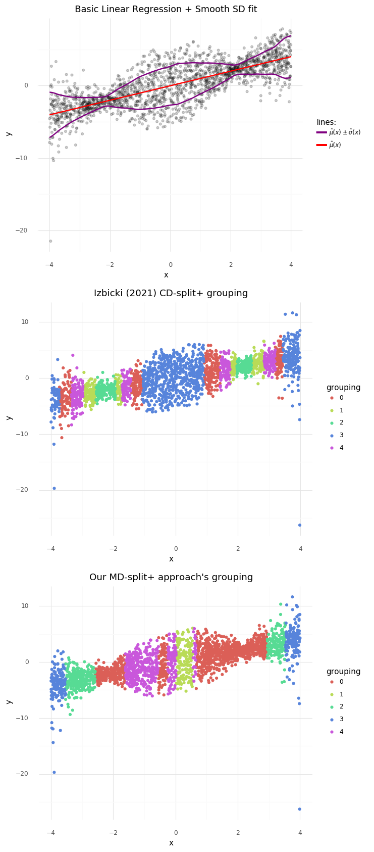
Figure 1: This figure relates to the example discussed in Section 4.1. The top subplot presents the underlying data distribution, as well as the fit of the mean and standard deviation that defines the CDE model. The lower two subplots display the local groupings for the local conformal approaches CD-split+ and MD-split+ with 5 clusters each. Notice that CD-split+ groups $X$ values with $Y$ that have a truncated normal together with $X$ values with $Y$ that have $t$-distributions with low degrees of freedom, and in general groups by $\sigma(x)$ values ($|X|-2$). This is not optimal, given that they have largely differing conformal score distributions. MD-split+ focuses more on grouping similar underlying distributions together.

For both procedures we create 5 partitions of the $\mathcal{X}$ space, and these can be seen in Figure 1’s lower two subplots This figure shows that the CD-split+ clusters utilizes the estimated $\hat{\sigma}(x)$ values (visually clustering by $|{\mathbf{x}}|$), whereas our approach uses the relative fit of the CDE model (visually clustering by $|{\mathbf{x}}|-2$). If we had also applied Lei and Wasserman [2014]’s approach, we would have seen clusters based solely on ${\mathbf{X}}$ value. Compared to CD-split+, our MD-split+ algorithm clusters with respect to the underlying distributional differences the data has. Compared to Lei and Wasserman [2014]’s, MD-split+ clusters more similar underlying residual distributions, by not being constrained to only cluster linearly on contiguous ${\mathbf{X}}$ values. This simple example highlights a drawback of clustering on model conditional density estimation when model fit is imperfect.

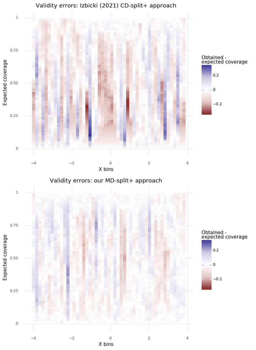
Figure 2: This figure captures the difference in empirical coverage and expected coverage for small bins on the $X$ space related to the generative distribution for example 1 and the clusters visualized in Figure 1. The top subplot relates to the CD-split+ approach with 5 clusters and the lower subplot relates to our proposed approach with 5 clusters as well.

In addition, this misspecified CDE model (Gaussian with varying mean and variance) means that as the number of observations ($n$) and the number of clusters ($k$) increases, we will not see asymptotic conditional validity emerge under CD-split+. Figure 2 captures the difference in local validity for a grid of small bins of $X$ values relative to both clustering approaches, with stronger colors highlighting large differences. As expected, CD-split+ performs worse on this localized level than our MD-split+ approach. In other words, a prediction region made using CD-split+ will more often have a different amount of conditional coverage than desired, and this difference will often be larger than that seen with prediction regions made using MD-split+.

4.2 Convolutional Neural Density Estimation for Galaxy Images

In this example, we consider the problem of estimating prediction regions for synthetic “redshift” values $Z$ (the response), which are assigned to photometric or “photo-z” galaxy images ${\mathbf{X}}$ (the features). Here, ${\mathbf{X}}$ represents a $20\times 20$-pixel image of an elliptical galaxy generated by GalSim, an open-source toolkit for simulating realistic images of astronomical objects [Rowe et al., 2015]. In GalSim, we can vary the axis ratio $\lambda$, defined as the ratio between the minor and major axes of the projection of the elliptical galaxy, as well as the galaxy’s rotational angle $\theta$ with respect to the x-axis. We create 9 equally sized populations of galaxies, representing every combination of $\lambda\in\{0.1,0.4,0.75\}$ and $\theta\in\{\pi/4,2\pi/3,5\pi/6\}$, with uniform noise added to $\lambda$ and $\theta$ for each individual image. See Figure 3 for representative examples of each galaxy image type.

Figure 3: We create 9 equally sized populations of galaxy images, representing combinations of axis ratios $\lambda\in\{0.1,0.4,0.75\}$ and angles $\theta\in\{\pi/4,2\pi/3,5\pi/6\}$. Individual images have a small amount of noise in both $\lambda$ and $\theta$. This grid shows a representative image from each group.

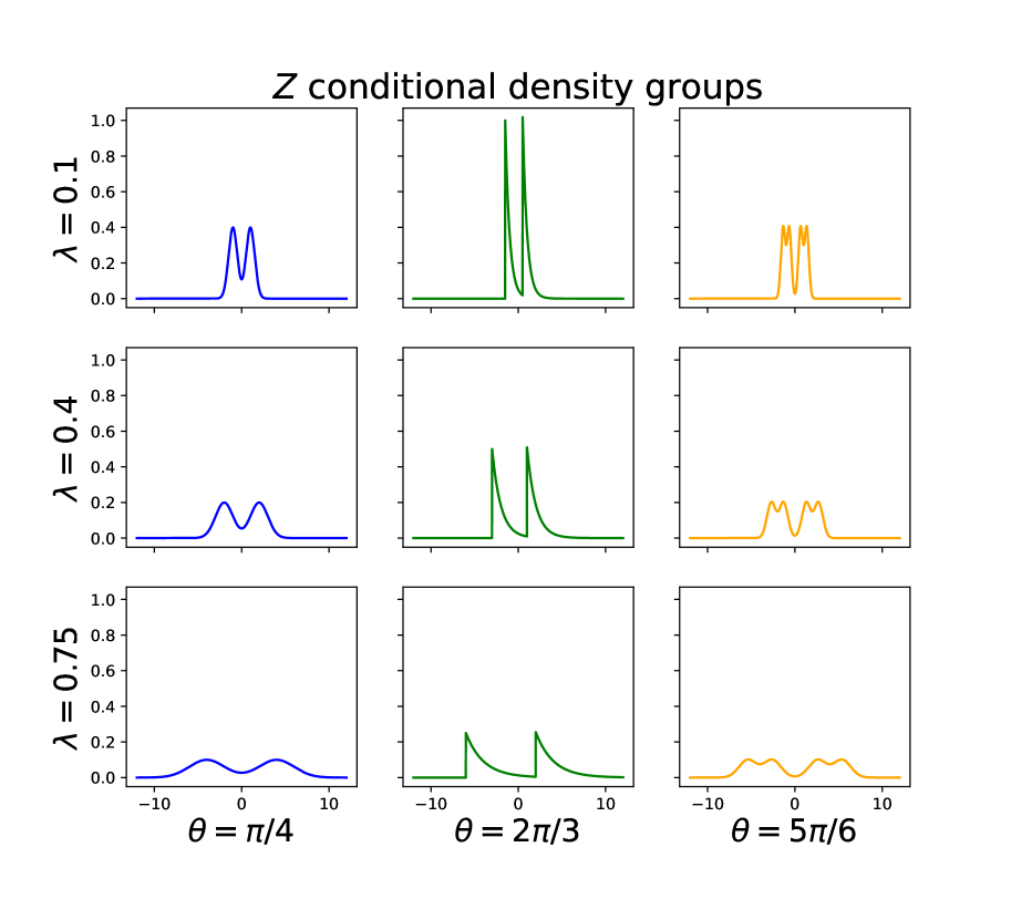
Figure 4: We define 9 conditional density models for the “redshift” $Z$, corresponding to the 9 galaxy image populations in Figure 3. Galaxy images with the same $\lambda$ value have densities $f(z|{\mathbf{x}})$ that have the same variance, while those with the same $\theta$ value have densities $f(z|{\mathbf{x}})$ that have the same distributional shape.

We then assign a response variable $Z$ with different bimodal mixture distributions as follows:

$$Z|\lambda,\theta\sim a_{\lambda}\left[\frac{1}{2}U_{\theta}+\frac{1}{2}V_{\theta}\right]$$

where

$$U_{\theta}=\begin{cases}\mathcal{N}(2,1),&\theta=\pi/4\\ \text{Exponential}(1)\text{ centered at 2},&\theta=2\pi/3\\ \frac{1}{2}\mathcal{N}(2.7,0.25)+\frac{1}{2}\mathcal{N}(1.3,0.25),&\theta=5\pi/6\end{cases}$$

$$V_{\theta}=\begin{cases}\mathcal{N}(-2,1),&\theta=\pi/4\\ \text{Exponential}(1)\text{ centered at -2},&\theta=2\pi/3\\ \frac{1}{2}\mathcal{N}(-2.7,0.25)+\frac{1}{2}\mathcal{N}(-1.3,0.25),&\theta=5\pi/6\end{cases}$$

and

$$a_{\lambda}=\begin{cases}0.5,&\lambda=0.1\\ 1,&\lambda=0.4\\ 2,&\lambda=0.75\end{cases}$$

See Figure 4 for a plot comparing these distributions.

Based on the marginal distribution of the response, a practitioner might reasonably decide to model conditional density estimates as a mixture of Gaussians. In particular, here we fit a Gaussian convolutional mixture density network (ConvMDN, [D’Isanto and Polsterer, 2018]), which can effectively train on the image feature space.

This is a situation where the data structure is more complex, so local conformal inference is challenging. Lei and Wasserman [2014]’s partitioning method does not scale well here because ${\mathbf{X}}$ is high-dimensional. Furthermore, we will demonstrate that even well-tuned, sophisticated conditional density models trained on this dataset with reasonably large sample sizes may be misspecified in subtle but fundamental ways. Thus, the methods of Izbicki et al. [2021] may not lead to sensible local subgroups. On the other hand, our proposed MD-split+ method provides a practical way to do local conformal inference successfully, even on complex data with imperfectly fit CDEs. In this example, we compare MD-split+ to the related approach CD-split+ [Izbicki et al., 2021].

For this complex data structure, we dedicate more data to training and validating the ConvMDN model. Specifically, for our MD-split+ implementation, we dedicate 27,000 observations to the training and validation sets (70/30 split), 4,500 observations for our diagnostic set (to train our HPD quantile functions), and 4,500 for the calibration set. For CD-split+ we add what was the diagnostic set above to the training and validation sets, thus giving us 31,500 observations (again with 70/30 split). We also evaluate both approaches on 4,500 test observations.

For both approaches, we fit a Gaussian convolutional mixture density network (ConvMDN, [D’Isanto and Polsterer, 2018]), with two convolutional and two fully connected layers with ReLU activations [Glorot et al., 2011]. We train these models using the Adam optimizer [Kingma and Ba, 2014] with learning rate $10^{-3}$, $\beta_{1}=0.9$, and $\beta_{2}=0.999$. We tune several hyperparameters in search of the best fitting ConvMDN model. We allow $M$, the number of mixture components, to vary from 2 to 10. We also tune the number of hidden units in the penultimate layer and whether to include dropout [Srivastava et al., 2014] after the convolutional layers. For both approaches, we found that the best ConvMDN model with the lowest KL loss had parameters $M=2$, 10 hidden layers, and a 50% dropout layer. For MD-split+ we also train a quantile regression model (with $\alpha\in\{0,0.02,....,1\}$) estimating $\widehat{HPD}(Y|{\mathbf{X}})$ values given ${\mathbf{X}}$, where $\widehat{HPD}$ is defined relative to the ConvMDN.

We then define three clusters of the calibration points using $d_{md}$ and $d_{profile}$ for MD-split+ and CD-split+ respectively. Next, we construct prediction regions on a test set of 4500 new observations (galaxy images + redshifts), and verify their coverage (whether the prediction region includes the true redshift). By construction, even this “best” ConvMDN model is misspecified, because the true conditional densities $f(z|{\mathbf{x}})$ are not all mixtures of 2 Gaussians. Therefore, simply using a distance that compares fitted CDE models $\widehat{f}$, as CD-split+ does, can lead to undesirable clusters that fail to achieve local conformal coverage on the true subpopulations of interest. In contrast, our method partitions the feature space into sensible regions, as the HPD distributions are the same across the scalings defined by $\lambda$. See Figure 5 for a comparison of the clusters achieved by these two methods.

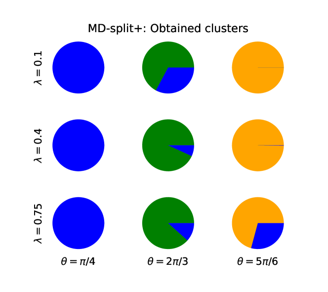
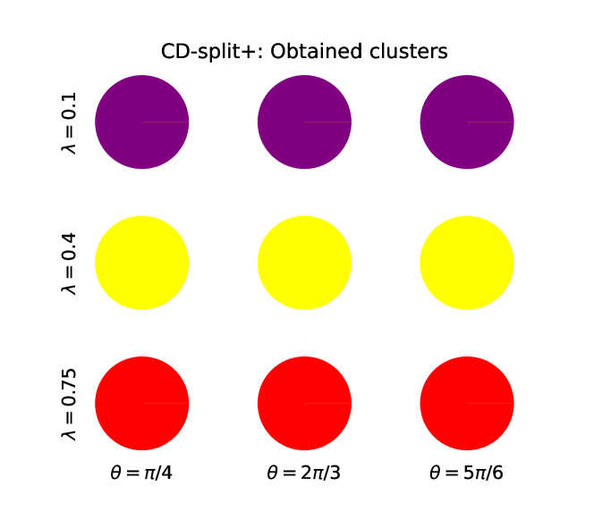
Figure 5: Pie charts showing the fraction of points assigned to different clusters. Top: Our method MD-split+ obtains reasonable clusters. For the most part, points with similarly shaped conditional densities (see Figure 4) are grouped together. Intuitively, such points will have similar HPD coverage profiles, and thus should belong to the same local conformal partition. Bottom: CD-split+ forms unintuitive clusters. This method clusters together distributions with the same variance, regardless of how differently shaped those distributions might be.

Next, we form local conformal prediction regions using the two sets of clusters and their associated conformal scores. Recall that CD-split+ uses conditional density estimate values, while MD-split+ uses $\widehat{HDP}$ values. Of course, by construction one will obtain validity on average over each cluster, for any arbitrary clusters one wishes to define. But we are interested in whether validity is achieved over the 9 true subpopulations in the dataset. Figure 6 shows the empirical coverage relative to the conformal confidence levels across the 9 true subpopulations. We see that, across the range of confidence levels, our method obtains empirical coverage very close to what is expected. On the other hand, CD-split+’s empirical coverage for these 9 true subpopulations varies drastically. Figure 7 shows this information for four specific confidence levels (0.2,0.4,0.6, and 0.8), again highlighting the performance differences between these two methods.

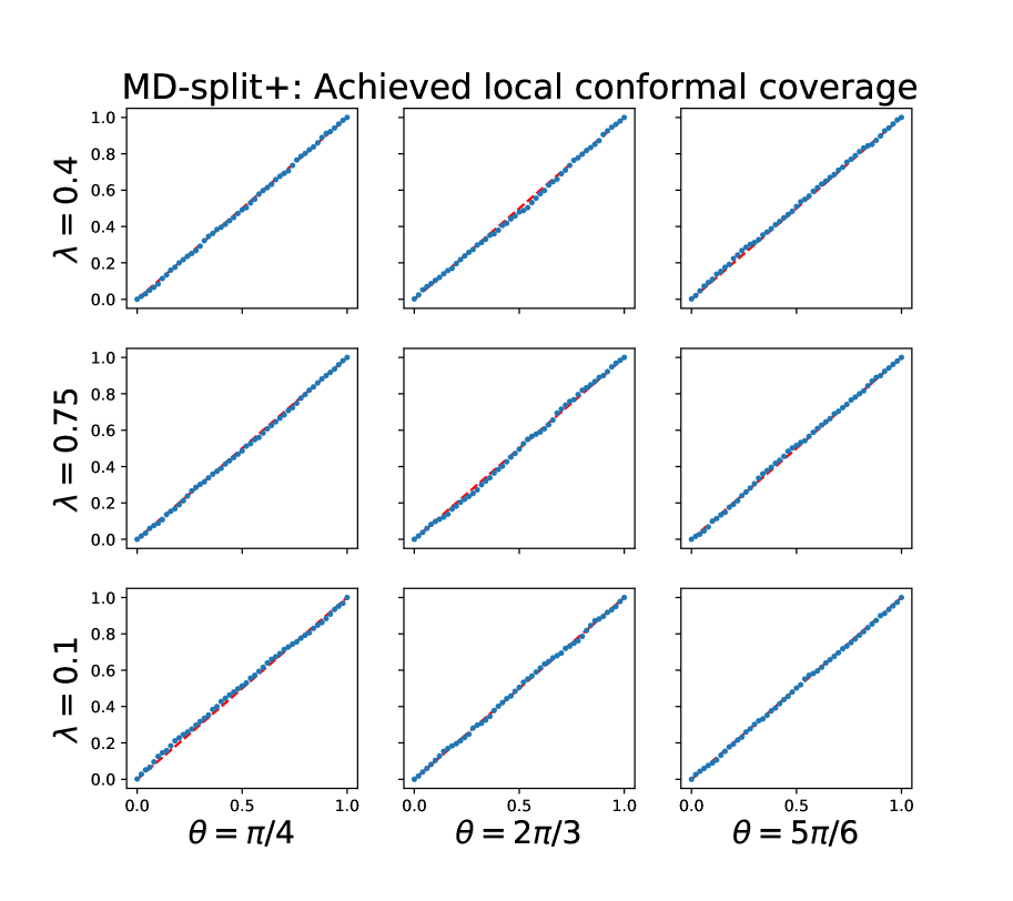
Figure 6: We check nominal vs. achieved coverage of local conformal sets within each of the 9 true subpopulations defined earlier. Top: Using the 3 clusters obtained from our method MD-split+, we achieve correct local conformal coverage across the range of $\alpha\in[0,1]$. Bottom: Using the 3 clusters obtained from CD-split+, we see clear deviations from correct local conformal coverage in many of the 9 true subpopulations.

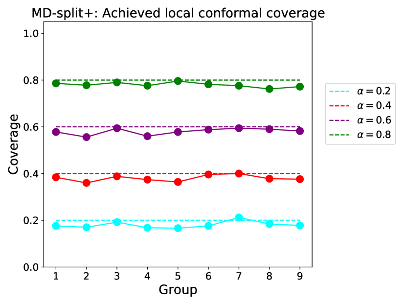
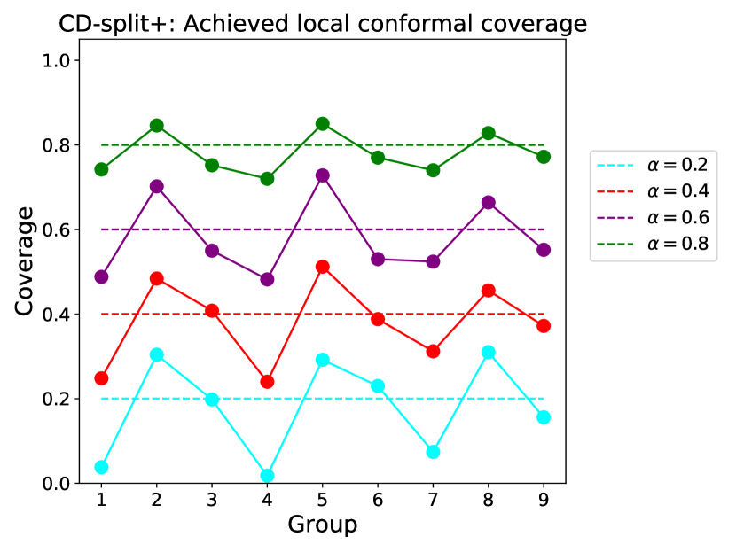
Figure 7: In this figure we select 4 particular confidence levels and check the achieved local conformal coverage by group, for nominal coverage levels of $\alpha=0.2,0.4,0.6,0.8$. Top: Our method MD-split+ achieves approximately correct coverage in every true subpopulation. Bottom: CD-split+ leads to large deviations from the correct coverage in most subpopulations. CD-split+ clusters together groups (1,2,3), (4,5,6), and (7,8,9) in the figure. While coverage is correct when averaged across these clusters, it is incorrect for the true groups of interest.

In this example, we have seen how a complex CDE model $\widehat{f}$ can remain misspecified, despite careful tuning. Moreover, this kind of misspecification would not be obvious to the practitioner. In theory, one can always simply “find a better model”, but in reality, models are often imperfect, especially in complex data settings. It is in this realistic context that MD-split+, unlike previous known methods, can still achieve valid, scalable local conformal inference.

5 Discussion

We have developed a novel local conformal inference method that is both scalable to high dimensions and extendable to complex data settings where conditional density estimators may be poorly estimated. As such, our method has great practical utility. If CDE models were always well fit, then the estimated conditional density level sets would always be close to the true level sets, and there would be no reason to use conformal inference at all. Instead, one could simply use the CDE model to select the level set with the probability mass equal to the desired confidence level.

In comparison with other local conformal inference techniques that use CDE or HPD values as their conformal scores, our approach does require an additional data split. However, the example in Section 4.2 shows that this added split will often not be too burdensome for the practitioner. In developing our approach, we observed the impact of having the CDE model or HPD quantile regression model not being well tuned. A poorly tuned CDE model (specifically one that is overfit), can make it harder for the HPD quantile regression function to correctly cluster ${\mathbf{X}}$ observations based on model performance. Similarly, a poorly tuned HPD quantile regression function can reduce the ability to obtain optimal clusters.

There is a lot of potential for future work in understanding the theoretical aspects and more nuanced properties of our approach. Specifically, we are interested in exploring whether our method achieves asymptotic conditional coverage with meaningfully weaker assumptions than, say, Izbicki et al. [2021]. We expect this to require understanding the smoothness in $\mathcal{X}$ of the true and estimated conditional density, as well as the smoothness in $\mathcal{X}$ of the oracle versus estimated HPD quantile regression function. Additionally, we seek to better understand (potentially empirically) how comparisons of our MD-split+ (with less data to train the estimated CDE model) to Izbicki et al. [2021]’s CD-split+ might change if, instead of fundamentally misspecified models, we had CDE and HPD quantile regression functions that were poorly fit due to finite sample sizes, but eventually converge to the true conditional density and oracle HPD quantile regression functions, respectively.

Overall, we see MD-split+ as a new tool in the practitioner’s toolkit for performing local conformal inference using conditional density estimation$-$one that is especially useful when $\mathcal{X}$ is high dimensional or the CDE is misspecified. We hope that our procedure will appeal to a wide range of practitioners, and that they will appreciate the philosophical foundations of our approach as one of its strengths.

6 Acknowledgements

BL and DZ are grateful for fruitful discussions with Aaditya Ramdas about this topic. BL would like to thank his advisor Chad Schafer for discussions on local conformal inference literature and potential extensions. DZ would like to thank his advisor Ann B. Lee and collaborator Rafael Izbicki, with whom he developed the conditional density model diagnostic tools leveraged in this paper.

References

- Barber et al. [2019] Rina Foygel Barber, Emmanuel J. Candès, Aaditya Ramdas, and Ryan J. Tibshirani. The limits of distribution-free conditional predictive inference. mar 2019. URL http://arxiv.org/abs/1903.04684.
- D’Isanto and Polsterer [2018] Antonio D’Isanto and Kai Lars Polsterer. Photometric redshift estimation via deep learning. generalized and pre-classification-less, image based, fully probabilistic redshifts. Astronomy & Astrophysics, 609:A111, 2018.
- Glorot et al. [2011] Xavier Glorot, Antoine Bordes, and Yoshua Bengio. Deep sparse rectifier neural networks. In Proceedings of the Fourteenth International Conference on Artificial Intelligence and Statistics, volume 15 of Proceedings of Machine Learning Research, pages 315–323, Fort Lauderdale, FL, USA, 11–13 Apr 2011. JMLR Workshop and Conference Proceedings.
- Guan [2019] Leying Guan. Conformal prediction with localization. arXiv preprint arXiv:1908.08558, 2019.
- Gupta et al. [2020] Chirag Gupta, Arun K. Kuchibhotla, and Aaditya K. Ramdas. Nested Conformal Prediction and quantile out-of-bag ensemble models. may 2020. URL http://arxiv.org/abs/1910.10562.
- Izbicki and Lee [2017] Rafael Izbicki and Ann B. Lee. Converting high-dimensional regression to high-dimensional conditional density estimation. Electronic Journal of Statistics, 11(2):2800–2831, 2017. ISSN 19357524. doi: 10.1214/17-EJS1302.
- Izbicki et al. [2021] Rafael Izbicki, Gilson Shimizu, and Rafael B. Stern. CD-split and HPD-split: efficient conformal regions in high dimensions. arXiv, pages 1–31, 2021. ISSN 23318422.
- Kingma and Ba [2014] Diederik P. Kingma and Jimmy Ba. Adam: A method for stochastic optimization. arXiv preprint arXiv:1412.6980, 2014.
- Lei and Wasserman [2014] Jing Lei and Larry Wasserman. Distribution-free prediction bands for non-parametric regression. Journal of the Royal Statistical Society. Series B: Statistical Methodology, 76(1):71–96, 2014. ISSN 13697412. doi: 10.1111/rssb.12021.
- Lei et al. [2013] Jing Lei, James Robins, and Larry Wasserman. Distribution-free prediction sets. Journal of the American Statistical Association, 108(501):278–287, 2013. ISSN 01621459. doi: 10.1080/01621459.2012.751873.
- Rowe et al. [2015] Barnaby Rowe, Mike Jarvis, Rachel Mandelbaum, Gary M. Bernstein, James Bosch, Melanie Simet, Joshua E. Meyers, Tomasz Kacprzak, Reiko Nakajima, Joe Zuntz, et al. GALSIM: The modular galaxy image simulation toolkit. Astronomy and Computing, 10:121–150, 2015.
- Srivastava et al. [2014] Nitish Srivastava, Geoffrey Hinton, Alex Krizhevsky, Ilya Sutskever, and Ruslan Salakhutdinov. Dropout: A simple way to prevent neural networks from overfitting. Journal of Machine Learning Research, 15(56):1929–1958, 2014. URL http://jmlr.org/papers/v15/srivastava14a.html.
- Vovk [2013] Vladimir Vovk. Conditional validity of inductive conformal predictors. Machine Learning, 92(2-3):349–376, 2013. ISSN 08856125. doi: 10.1007/s10994-013-5355-6.
- Vovk et al. [2005] Vladimir Vovk, Alex Gammerman, and Glenn Shafer. Algorithmic Learning in a Random World. Springer Science & Business Media, 2005. ISBN 0-387-00152-2.
- Zhao et al. [2021] David Zhao, Niccolò Dalmasso, Rafael Izbicki, and Ann B. Lee. Diagnostics for conditional density models and Bayesian inference algorithms. In Proceedings of the 37th Conference on Uncertainty in Artificial Intelligence (UAI), volume 125 of Proceedings of Machine Learning Research. PMLR, 26–29 Jul 2021.